Astronomy 330 Lecture 3 10 Sep 2010

  Review & a little more on reionization   Stellar Classification

  Photometry/classification   Stellar Evolution   Interpreting H-R diagrams   Reading: “Old Main Sequence Turnoff Photometry in the

Small Magellanic Clouds” Noël et al. (2007, AJ, 133, 2037)   What is the data they use?   Compare Figures 3 and 7 to some of the CMDs in the lecture

notes – what are the similarities and differences?

Outline

Review: Big Bang / Creation of Matter

  Expansion & evolution: GR and Friedman equations: R=1/1+z, R,R

  Early Universe   Inflation (10-34 sec)   Particle genesis (10-15 to 1 sec)   BBNS (3 minutes) Cosmic He abundances   Recombination (4x105 yr) CMBR

  Dark Ages (?)   Reionization and onward

  When the first stars and AGN formed (z=12?)   Galaxy formation   Evolution of galaxies, their stars and planets

precision cosmology

& first glimpse of structure

radn dom.

matterdom.

Structure grows via gravity in matter dominated era

. ..

Structure starts growing here

reionization:

Epoch of Reionization

  Somehow, somewhere stars formed…   …and ionized the surrounding IGM and

the Universe emerged out of the “Dark Ages”

  WMAP says somewhere near z~12…   But possibly two phases, one early (z>12,

and incomplete)   When did the 1st stars/galaxies form?

  Gunn-Peterson trough in quasar absorption   Directly observing 1st stars (NGST, TMT)   21 cm line absorption/redshifted emission

(SKA)   High redshift objects (VLA, GMRT, SKA)   Primordial, high redshift black holes (SKA)

21 cm Observations: Emission

Furlanetto et al. 2004

z = 12.1 z = 9.2 z =7.6

10 Mpc comoving Δν= 0.1 Mhz

Large scale structure: simulated

  Fly-through of the Cosmic Web

Large Scale Structure: observed   Filaments and voids

o  Great Attractor o  Characteristic scales: 40-120 Mpc

Large scale structure of the Universe

  Structure and Galaxy Formation elliptical

spiral

The WHIM: Warm-Hot Intergalactic Medium

WHIM

T/106 K

Dark matter

density

Physical Processes in the Cosmic Web

  Large scale shocks as baryons accrete onto collapsing structures

  Gas is shock-heated to 105-107 K   WHIM origins, or AGN and star-formation too?

  Shock accelerate particles (cosmic ray ions) to 1018–1019eV

  Inter-cluster B-fields: 10-7–10-12 G   Origin and amplification?

Mapping the Cosmic Web   Galaxies are only the high density islands in the web   Most of the web is in the form of diffuse WHIM

  Detected primarily via QSO absorption sightlines   Fraction of kinetic power converted to radiative energy

  Diffuse emission should be detectable in the optical (nebular line emission, e.g., redshifted Lyα) but suitable instrumentation has yet to be built.

  Diffuse synchotron emission (radio) another possibility   Parameters:

  Infall velocity   Density of in-falling baryonic gas   Magnetic field strength   Efficiency of shock acceleration   Fraction of kinetic power converted to radiative energy

Furlanetto et al. 2003: Ly α surface-brightness

  Dynamics   Stars are point masses –

  collisionless tracers of the potential   Distinctions between stars irrelevant

  But, which stars most accurately trace the “true” morphology and dynamics of a galaxy?

  Chemical evolution   Stars are responsible for producing and distributing the

elements   Metric of evolution

  Star formation rate (SFR)   Star formation history (SFH)

  H-R diagram are all diagnostics of evolution   Feedback

  evolution/organization of ISM in galaxies driven by gravity, hydrodynamics, and input of energy from stars

Role of Stars in Extragalactic Astronomy

Digression & Review: Flux Units

  Flux (fν): measured in Janskys   1 Jy = 10-26 W m-2 Hz-1= 10-23 erg sec-1 cm-2 Hz-1

  Flux (fλ): measured in ergs s-1 cm-2 A-1 (cgs units)   Photon flux (fγ) is useful for calculating signal-to-

noise (counting statistics):  Define neper = Δλ/λ = Δν/ν = Δln ν   The photon flux is:

  photons sec-1 cm-2 neper-1 = fν/h   where h=6.6256 x 10-27 erg sec

  Useful identify:

1 microJy = µJy = 15.1 photons sec-1 m-2 neper-1

Apparent magnitudes

€

m1 −m2 = −2.5log10f1f2

⎛

⎝ ⎜

⎞

⎠ ⎟ = −aln

f1f2

⎛

⎝ ⎜

⎞

⎠ ⎟

a = 2.5log10 e =1.08574

m = −2.5log10f1f0

⎛

⎝ ⎜

⎞

⎠ ⎟ + m0

m0 : zeropoint of the magnitude system

Pogson’s ratio (MNRAS, 1856, 17, 12)

fn: the apparent flux of object n.

Will drop “10” here on out.

f = f0 dexp[ -0.4(m-m0)] how to get your money back

Absolute Magnitudes

  Absolute magnitude is the apparent magnitude that would be observed if the object were at a distance, d, of 10 pc.

  Aλ is the total extinction due to interstellar dust, in magnitudes, typically take to be only the Galactic foreground screen (Burstein & Heiles 1982, AJ, 87, 1165; Schlegel et al. 1998, ApJ, 500, 525):

  f = f0 exp(-τλ) ,   Aλ = 1.086 τλ = -2.5 log( f/f0)

€

mλ −Mλ = 5log10 d − 5 + Aλ

∴f1f2

=d2d1

⎛

⎝ ⎜

⎞

⎠ ⎟

2

HI

IRAS

See nedwww.ipac.caltech.edu/help/extinction_law_calc.html

Absolute Magnitudes

  For extragalactic observers: d in Mpc, plus the so-called k-correction, κ, which accounts for effects of the cosmological expansion

1)  effects of redshifting the rest-frame spectrum in the observed band-pass; and

2)  photon dilution.

€

mλ −Mλ = 5log10 d + 25 + Aλ +κλ

See, e.g.: Schneider, Gunn & Hoessel (1983, ApJ, 264, 337)

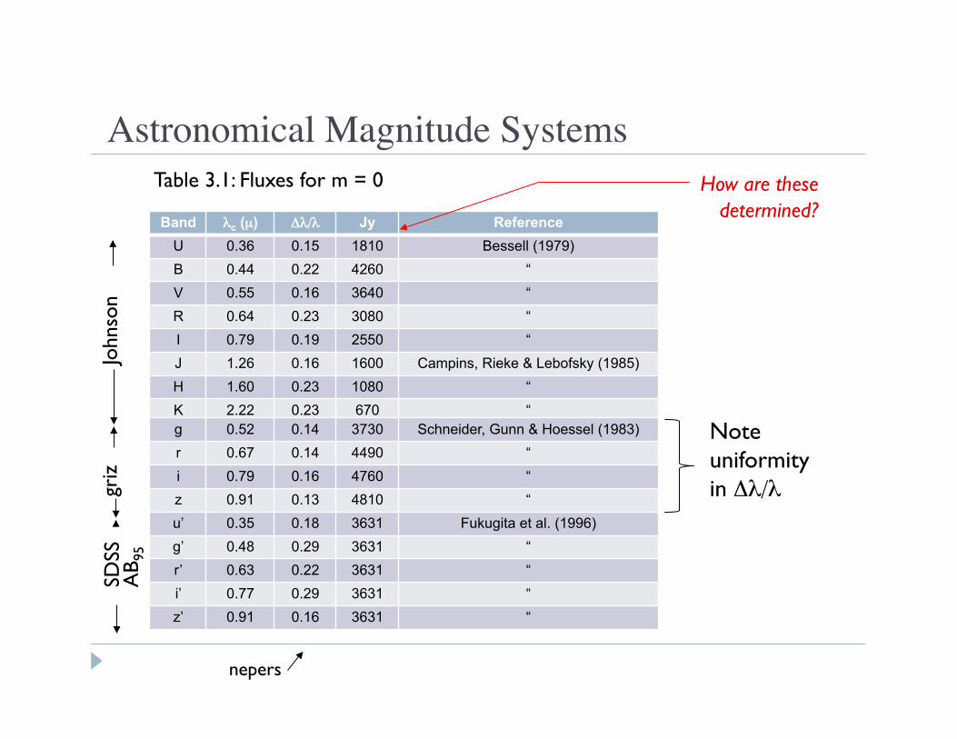
Astronomical Magnitude Systems

Band λc (µ) Δλ/λ Jy Reference

U 0.36 0.15 1810 Bessell (1979)

B 0.44 0.22 4260 “

V 0.55 0.16 3640 “

R 0.64 0.23 3080 “

I 0.79 0.19 2550 “

J 1.26 0.16 1600 Campins, Rieke & Lebofsky (1985)

H 1.60 0.23 1080 “

K 2.22 0.23 670 “ g 0.52 0.14 3730 Schneider, Gunn & Hoessel (1983)

r 0.67 0.14 4490 “

i 0.79 0.16 4760 “

z 0.91 0.13 4810 “

u’ 0.35 0.18 3631 Fukugita et al. (1996)

g’ 0.48 0.29 3631 “

r’ 0.63 0.22 3631 “

i’ 0.77 0.29 3631 “

z’ 0.91 0.16 3631 “

How are these determined?

Note uniformity in Δλ/λ

Table 3.1: Fluxes for m = 0

nepers

John

son

griz

SD

SS

AB 9

5

  Photometry : Based on optical and near-infrared (NIR) colors   First order: stars are blackbodies, so any two

flux-points constrain temperature   Combination of two bands yield “color” =

temperature   Second-order: stars have line-blanketing, so

e.g., colors are degenerate for massive stars   Need observations in at least three bands.   NIR can break degeneracy between cool

giants and dwarfs.

  Spectroscopy : individual line ratios very tightly constrain temperature, surface gravity, etc.   Yields the OBAFGKM classification   Further sub-classification is the luminosity class

Stellar Classification

Nicolet (1980)

Bessell & Brett (1988)

Interstellar redening

Line-blanketing from H Balmer series

dwarfs

giants

U-B

B-V

Basic Properties of Stars (chapter 1.1)

Spec. type

Absorption lines

Teff (K) Mv (V, I) (B-V)

O He II, C III 40-50,000 -6,-8 <-0.33

B He I, S III, H 12-30,000 -1.5, -7 -0.2

A H, Mg II 7-9,000 1.0, -7 0

F Ca II 6-7,000 3.0,-7 0.4

G Ca II, CH 5.5-6,000 5.0,-7 0.6

K CH, CN 4-5,500 6.0,-7 1.2

M TiO 2.5-4000 9.0,-7 1.6

  Ia – most extreme supergiants   Ia – moderate supergiants   Ib – less luminous supergiants   II – bright giants   III – normal giants   IV – subgiants   V - dwarfs

Luminosity class

Kaler 2006

x104

  History: BBNS cannot account for the abundances of all the elements; Burbridge, Burbridge, Fowler, & Hoyle laid out the model for stellar nucleosynthesis.

  Main sequence: H to He fusion via proton-proton chain & CNO bi-cycle

  Post-MS: H depletion in core, interior pressure decreases, collapse of core and interior, H shell burning ignites, envelope expands and star becomes a red giant.

  Later phases: repeat with heavier and heavier elements via α-processes, faster and faster rates (more energy production per unit time), more and more shells.

  Fusion ends depending on mass sufficient to overcome core degeneracy, or when core burns to Fe.

Fundamentals of Stellar Evolution

  Because H burning lifetime depends on mass there is a nice correlation between turn-off mass and age   Spectral types are determined by surface-temperature (Teff)   Teff set by mass on the main sequence:   more mass burns brighter and hotter

  LMS/L ~ (M/M)2.14 (M/M > 20)   LMS/L ~ (M/M)3.5 (2 < M/M < 20)   LMS/L ~ (M/M)4.8 (M/M < 2)

MS Stellar Lifetimes

So: τMS = 10 (M/M)(L/L)-1 Gyr  

  RGB to Horizontal Branch (HB)   Core contraction/core mass increases   T~108 K, ρ ~ 104 g cm-3 get He

burning   2α → 8Be, 8Be + α → 12C   In stars w/ M > 2M, its not degenerate

and we get core expansion   Essentially a He-burning main sequence   In more massive stars get 12C + α →

16O; for stars with M up to 8 M we’re left with a degenerate CO core (white dwarf)  

  He-burning lifetime ~108 years   Evolution to Asymptotic Giant Branch

(M > 8 M)   Further Burning Stages…

Post-MS Stellar Evolution

  Evolution to AGB   He-burning, growing CO core

  Low mass stars can’t lift degeneracy, end up as planetary nebula + white dwarf

  Eventually get He shell burning that drives expansion of envelope and luminosity increases (plus unburned H, H shell burning)   Occurs with a series of “dredge-ups” that

produce chemically bizarre stars (convection)   Site of “s-process” nucleosynthesis

Fundamentals of Stellar Evolution

  Neutron capture processes   S-process (“slow”) – yields elements like Ba and Tc largely in AGB stars

(all those free n from previous burning processes)   R-process (“rapid”) – yields very heavy elements like Ur, usually in SNe

  Further Burning Stages   12C + 12C → 20Ne + α   16O + 16O → 28Si + α   20Ne + 4He → 24Mg + γ   Leads ultimately to the production

of 56Fe, core collapse, and supernova explosion (Type II SNe)

  Can also get n production via, e.g., 12C + 12C → 23Na + n  

Fundamentals of Stellar Evolution

  Color – temperature – mass – lifetime relationships mean the observed “color-magnitude” diagram (CMD) can tell us something about the age/evolutionary status of a stellar population (especially if it’s a single age)

  CMD can also hint at the production of metals

Understanding Stellar Populations

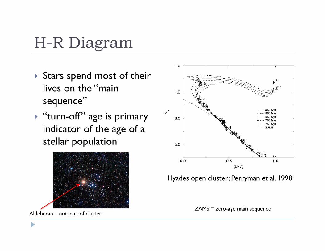
H-R Diagram

  Stars spend most of their lives on the “main sequence”

  “turn-off” age is primary indicator of the age of a stellar population

Hyades open cluster; Perryman et al. 1998

Aldeberan – not part of cluster ZAMS = zero-age main sequence

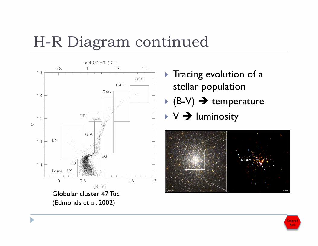
H-R Diagram continued

  Tracing evolution of a stellar population

  (B-V) temperature   V luminosity

Globular cluster 47 Tuc (Edmonds et al. 2002)

Stopped here

H-R Diagram

  Gets more complicated with a mixed-age stellar population

  Multiple turn-offs, multiple HBs

  Dwarf spheroidal galaxies are ideal labs for this

  Stellar initial mass function   dN = Noξ(M)dM   No ∫ dM M ξ(M) = total mass of burst/episode   Observationally: ξ(M) goes as (M/M)-2.35

  “Salpeter IMF”    Slight variation with mass (time? environment?), according to some   Upper mass limit in the 80-120 M%

  but note small-number statistics become important %  Turn-over likely below 0.1 M%

Statistical Stellar Astrophysics

  Integrated Colors   Population I – “Disk Population” – open clusters, circular orbits, confined

to a disk, “blue”   Population II – “Halo Population” – globular clusters, large random

velocities, elliptical orbits, spherical distribution, “red”   Population III – extremely metal poor, not yet detected

  Cosmic Mystery #2: Where are the Pop-III stars?

  Correlations   Color vs kinematics

  Blue stars are disk-like   Color vs metallicity

  Red stellar populations tend to be metal poor, strong Galactic correlation between kinematics and metallicity

Stellar Populations

  Density of any locale on a CMD is a function of IMF, SFR, mass, and age   C(MV, V-I) = ∫∫ξ(log m, t) x SFR(t) dt dlogm

  Small mass bin (i.e. single mass)   Constant IMF (ξ)    Can recover star formation history from a complex CMD  

  Statistical Approach   What is the probability that a certain distribution of points on the

CMD came from one particular set of stellar evolution models (Tolstoy & Saha 1996)

Interpretting CMDs