A&A 540, A86 (2012)DOI: 10.1051/0004-6361/201118525c© ESO 2012

Astronomy&

Astrophysics

Chromospheric backradiation in ultraviolet continua and Hα

R. J. Rutten1,2,3,� and H. Uitenbroek4

1 Sterrekundig Instituut, Utrecht University, Postbus 80 000, 3508 TA Utrecht, The Netherlandse-mail: r.j.rutten@uu.nl

2 Institute of Theoretical Astrophysics, University of Oslo, PO Box 1029, Blindern, 0315 Oslo, Norway3 Lockheed-Martin Solar and Astrophysics Laboratory, 3251 Hanover Street, Palo Alto, CA 94304, USA4 National Solar Observatory /Sacramento Peak��, PO Box 62, Sunspot, NM 88349, USA

Received 26 November 2011 / Accepted 29 February 2012

ABSTRACT

A recent paper states that ultraviolet backradiation from the solar transition region and upper chromosphere strongly affects the degreeof ionization of minority stages at the top of the photosphere, i.e., in the temperature minimum of the one-dimensional static modelatmospheres presented in that paper. We show that this claim is incompatible with observations and we demonstrate that the pertinentionization balances are instead dominated by outward photospheric radiation, as in older static models. We then analyze the formationof Hα in the above model and show that it has significant backradiation across the opacity gap by which Hα differs from other strongscatttering lines.

Key words. radiative transfer – Sun: UV radiation – Sun: chromosphere

1. Introduction

Static one-dimensional (1D) modeling of the solar atmo-sphere assumes hydrostatic equilibrium in plane-parallel-layergeometry to deliver temperature and density stratifications alongvertical columns that may serve as reference description to com-pute spectral continua and lines similar to actual solar radia-tion. Early versions of such “standard” models were compiled byde Jager (1959) and Heintze et al. (1964a,b). Holweger’s (1967)LTE best-fit to optical iron lines became the first choice in clas-sical abundance determination, in particular as the HOLMULupdate by Holweger & Müller (1974). This model describesonly the photosphere and is close to theoretical photospheremodels based on the additional assumption of energy con-servation in the form of radiative equilibrium plus mixing-length convection in the deepest layers (e.g., Kurucz 1974,1994; Gustafsson et al. 1975, 2008). Semi-empirical best-fitmodeling of solar continua including ultraviolet wavelengthssampling the chromosphere continued with the BilderbergContinuum Atmosphere (Gingerich & de Jager 1968), theHarvard-Smithsonian Reference Atmosphere (Gingerich et al.1971), the VAL model grids of Vernazza et al. (1973, 1976,1981) fitting disk-center Lyman brightness bins, the update byMaltby et al. (1986), the more recent update concentrating ondisk-center ultraviolet spectra by Avrett & Loeser (2008), andthe sequence of similar refinements by Fontenla et al. (1990,1991, 1993, 2002, 2006, 2007, 2009).

This paper is triggered by the conclusion of Fontenla et al.(2009) that “in the solar chromosphere, the FUV and EUVobserved emissions in continuum and lines produced in theupper chromosphere and transition region irradiate the low

� Lingezicht Astrophysics, ’t Oosteneind 9, 4158CA Deil, TheNetherlands.�� Operated by the Association of Universities for Research inAstronomy, Inc. (AURA), for the National Science Foundation.

chromosphere and have significant effects on the ionization”.In particular, they claim that such backradiation strongly af-fects the density of minority stages of ionization in and near thetemperature minimum of their quiet-Sun model. We first showthat this claim is incompatible with basic observations, and thenuse illustrative computations to demonstrate that, instead, pho-tospheric irradiation from below is the dominant agent in ultra-violet continuum formation in the quiet-Sun model of Fontenlaet al. (2009), as was the case for the older standard models.

We continue by demonstrating that significant chromo-spheric backradiation occurs in Hα in such static models throughtwo-level scattering (Sect. 6), but argue that the assumption ofcolumnar hydrostatic equilibrium is untenable for the chromo-sphere and transition region (Sect. 7).

2. Observation

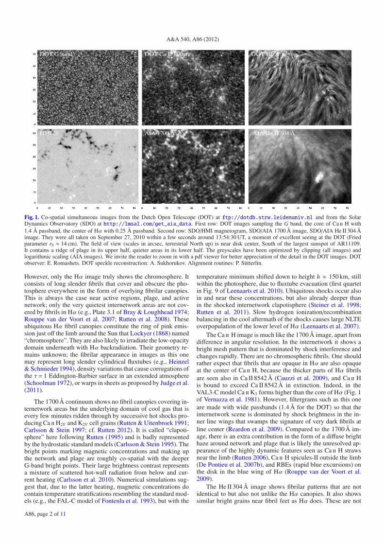
In this section we briefly review the observational character ofthe chromosphere, as counterpart to the standard-model defini-tion as the domain between the model’s temperature minimumand steep temperature rise toward the corona. Figure 1 gives anoverview of the appearance of the solar atmosphere in an areacontaining plage and network. We use it to demonstrate that theactual chromosphere may have enough opacity to supply signif-icant backradiation in Hα, but not in the 1700 Å continuum.

The G-band image and the magnetogram in the first columnof Fig. 1 are photospheric. The first image displays the gran-ulation and the spatial distribution of small kilogauss magneticconcentrations qualitatively and without sign through their proxyas intergranular bright points (best seen when zooming in). Thesecond image quantifies the actual surface distribution of theline-of-sight component in such strong-field concentrations, butat lower angular resolution. The correspondence is excellent.

The other four images allegedly sample the chromosphere(1700 Å, Ca ii H, Hα) and the transition region (He II 304 Å).

Article published by EDP Sciences A86, page 1 of 11

A&A 540, A86 (2012)

Fig. 1. Co-spatial simultaneous images from the Dutch Open Telescope (DOT) at ftp://dotdb.strw.leidenuniv.nl and from the SolarDynamics Observatory (SDO) at http://lmsal.com/get_aia_data. First row: DOT images sampling the G band, the core of Ca ii H with1.4 Å passband, the center of Hα with 0.25 Å passband. Second row: SDO/HMI magnetogram, SDO/AIA 1700 Å image, SDO/AIA He II 304 Åimage. They were all taken on September 27, 2010 within a few seconds around 13:54:30 UT, a moment of excellent seeing at the DOT (Friedparameter r0 ≈ 14 cm). The field of view (scales in arcsec, terrestrial North up) is near disk center, South of the largest sunspot of AR11109.It contains a ridge of plage in its upper half, quieter areas in its lower half. The greyscales have been optimized by clipping (all images) andlogarithmic scaling (AIA images). We invite the reader to zoom in with a pdf viewer for better appreciation of the detail in the DOT images. DOTobserver: E. Romashets. DOT speckle reconstruction: A. Sukhorukov. Alignment routines: P. Sütterlin.

However, only the Hα image truly shows the chromosphere. Itconsists of long slender fibrils that cover and obscure the pho-tosphere everywhere in the form of overlying fibrilar canopies.This is always the case near active regions, plage, and activenetwork; only the very quietest internetwork areas are not cov-ered by fibrils in Hα (e.g., Plate 3.1 of Bray & Loughhead 1974;Rouppe van der Voort et al. 2007; Rutten et al. 2008). Theseubiquitous Hα fibril canopies constitute the ring of pink emis-sion just off the limb around the Sun that Lockyer (1868) named“chromosphere”. They are also likely to irradiate the low-opacitydomain underneath with Hα backradiation. Their geometry re-mains unknown; the fibrilar appearance in images as this onemay represent long slender cylindrical fluxtubes (e.g., Heinzel& Schmieder 1994), density variations that cause corrugations ofthe τ= 1 Eddington-Barbier surface in an extended atmosphere(Schoolman 1972), or warps in sheets as proposed by Judge et al.(2011).

The 1700 Å continuum shows no fibril canopies covering in-ternetwork areas but the underlying domain of cool gas that isevery few minutes ridden through by successive hot shocks pro-ducing Ca iiH2V and K2V cell grains (Rutten & Uitenbroek 1991;Carlsson & Stein 1997; cf. Rutten 2012). It is called “clapoti-sphere” here following Rutten (1995) and is badly representedby the hydrostatic standard models (Carlsson & Stein 1995). Thebright points marking magnetic concentrations and making upthe network and plage are roughly co-spatial with the deeperG-band bright points. Their large brightness contrast representsa mixture of scattered hot-wall radiation from below and cur-rent heating (Carlsson et al. 2010). Numerical simulations sug-gest that, due to the latter heating, magnetic concentrations docontain temperature stratifications resembling the standard mod-els (e.g., the FAL-C model of Fontenla et al. 1993), but with the

temperature minimum shifted down to height h ≈ 150 km, stillwithin the photosphere, due to fluxtube evacuation (first quartetin Fig. 9 of Leenaarts et al. 2010). Ubiquitous shocks occur alsoin and near these concentrations, but also already deeper thanin the shocked internetwork clapotisphere (Steiner et al. 1998;Rutten et al. 2011). Slow hydrogen ionization/recombinationbalancing in the cool aftermath of the shocks causes large NLTEoverpopulation of the lower level of Hα (Leenaarts et al. 2007).

The Ca ii H image is much like the 1700 Å image, apart fromdifference in angular resolution. In the internetwork it shows abright mesh pattern that is dominated by shock interference andchanges rapidly. There are no chromospheric fibrils. One shouldrather expect that fibrils that are opaque in Hα are also opaqueat the center of Ca ii H, because the thicker parts of Hα fibrilsare seen also in Ca II 8542 Å (Cauzzi et al. 2009), and Ca ii His bound to exceed Ca II 8542 Å in extinction. Indeed, in theVAL3-C model Ca iiK3 forms higher than the core of Hα (Fig. 1of Vernazza et al. 1981). However, filtergrams such as this oneare made with wide passbands (1.4 Å for the DOT) so that theinternetwork scene is dominated by shock brightness in the in-ner line wings that swamps the signature of very dark fibrils atline center (Reardon et al. 2009). Compared to the 1700 Å im-age, there is an extra contribution in the form of a diffuse brighthaze around network and plage that is likely the unresolved ap-pearance of the highly dynamic features seen as Ca ii H strawsnear the limb (Rutten 2006), Ca ii H spicules-II outside the limb(De Pontieu et al. 2007b), and RBEs (rapid blue excursions) onthe disk in the blue wing of Hα (Rouppe van der Voort et al.2009).

The He II 304 Å image shows fibrilar patterns that are notidentical to but also not unlike the Hα canopies. It also showssimilar bright grains near fibril feet as Hα does. These are not

A86, page 2 of 11

R. J. Rutten and H. Uitenbroek: Chromospheric backradiation

cospatial with the bright grains in the G-band and Ca ii H im-ages. The overall similarity suggests that hot transition-regiongas shares the field-guided topography of the Hα chromosphere,outlining similar magnetic connectivity patterns. Such patternsseem also to be mapped by Lyα fibrils in VAULT images(Vourlidas et al. 2010). Any fibril that is opaque in Hα must bevery thick in Lyα but, comparably to Ca ii H, the cell-coveringfibrils are very dark in Lyα whereas other structures, likelyDoppler-shifted out of line-center obscuration, contribute largerbrightness in the profile-summed VAULT images (Koza et al.2009).

The conclusion from this section is that significant chromo-spheric backradiation may be expected in Hα and in He II 304 Åwhich show opaque fibrilar canopies that constitute the actualchromosphere. Ca ii H should show them too at line center, butthe DOT image and all other H & K filtergrams have too wide abandpass. In the 1700 Å image the absence of any fibrilar signa-ture, bright or dark or as erasure of the internetwork pattern seenin Ca ii H, implies that they are transparent at this wavelength,even for such a not-so-quiet area. Since the backradiation by anoptically thin fibril scales with the fibril opacity, it is unlikelythat deeper layers are affected by chromospheric backradiationin such ultraviolet continua.

3. Formulation

Fontenla et al. (2009) based their claim of important chromo-spheric backradiation on their Fig. 4 containing graphs of pop-ulation departure coefficients b for selected levels of Si i, Si ii,Mg i, MgII, Fe i, and Fe ii. Population departure coefficients mea-sure the ratio of the actual population density (particles cm−3) tothe population computed assuming LTE. There are two formatsdiffering in normalization. The first, called “Menzel” here, fol-lows the original use by Menzel & Cillié (1937) who normalizedhydrogen populations to the free proton density. The general-ization is to use a partial Saha-Boltzmann evaluation to obtainnormalization to the next ion stage (Eq. (6.3) of Jefferies 1968;Eqs. (13)–(15) of Vernazza et al. 1981). The other format, called“Zwaan” here, follows Wijbenga & Zwaan (1972) and uses theelemental abundance as normalization. The two conventions are(Rutten 2003):

bZwaani ≡ ni/n

LTEi and bMenzel

i ≡ ni/nLTEi

nC/nLTEC

, (1)

where ni is the population of level i, nC is the total population ofthe next ion, and the superscript LTE implies a complete solutionof the Boltzmann-Saha LTE partitioning equations for the givenlevel and all stages of the element. Sometimes the ion groundstate nc is used instead of nC assuming nc ≈ nC . When the atomor ion containing level i is predominantly ionized, so that nC ≈nLTE

C because most particles of the species are in the next-ionstage, then

bMenzeli ≈ ni/n

LTEi ≈ bZwaan

i , (2)

but when most of the element sits in level i itself then

bMenzeli ≈ nLTE

C /nC ≈ 1/bZwaanC . (3)

The continuum has bMenzelC ≡ 1 and the ratio bi/bC ≈ bi/bc is the

same in both definitions.Equations (2) and (3) were given as Eqs. (17) and (18)

by Vernazza et al. (1981), who used the Menzel definition.

Fig. 2. Temperature stratification in some standard models. Solid: FAL-C of Fontenla et al. (1993). Dot-dashed: its AL-C7 update by Avrett &Loeser (2008). Dashed: FCHHT-B of Fontenla et al. (2009). Dotted:radiative-equilibrium model from Kurucz (1979, 1992a,b), extended tolarger height assuming constant temperature.

Fontenla et al. (2009) did so too (Fontenla, priv. comm.). Weshow results for both definitions here because the Zwaan ver-sion gives a more intuitive display of actual population depar-tures for majority stages. For example, the Menzel-coefficientdips for n = 1 of H i and C i at the temperature minimum inFigs. 30 and 33 of Vernazza et al. (1981) and Figs. 13 and 14 ofFontenla et al. (2007) do not imply that the populations of theselevels are out of LTE.

4. Demonstration

We select magnesium for plotting departure coefficients as inFig. 4 of Fontenla et al. (2009). Magnesium is an importantelectron donor in the upper photosphere where Mg i has largerRydberg populations than any other element (Fig. 15 of Carlssonet al. 1992). It has important bound-free edges, at 1621.5 Å (vac-uum) from the ground state (3s2 1Se) and especially at 2512.4 Å(air) from the first excited level (3s3p 3P). Mg i and Mg ii spec-trum formation are characteristic for other abundant metals withlow ionization energy (silicon, iron, aluminum). Together, thesesupply the electrons for the photospheric H− opacity in the vis-ible and infrared and they dominate the solar continuous opac-ity from the near-ultraviolet to Lyα (Fig. 36 of Vernazza et al.1981).

Figure 2 displays a selection of standard models. FAL-C ofFontenla et al. (1993) was an update of VAL3-C of Vernazzaet al. (1981) with a less steep upper photosphere from the inclu-sion of the ultraviolet line haze and a different transition regionfrom the inclusion of ambipolar diffusion. A more recent updateis the AL-C7 model of Avrett & Loeser (2008), constructed inparticular to reproduce the ultraviolet spectrum atlases of Brekke(1993) and Curdt et al. (2001). These spectra are also repro-duced by model FCHHT-B of Fontenla et al. (2009), which hasa higher-located temperature minimum to accommodate dark in-frared CO lines.

The dotted curve in Fig. 2 is a radiative-equilibrium modelfrom Kurucz (1979, 1992a,b), that we extended in Cauzzi et al.(2009) to larger height assuming constant temperature. It is verysimilar to the FCHHT-B model up to h = 800 km, but has nochromosphere or transition region and so serves as comparisonfor the case of no backradiation whatsoever.

We have used the 1D version of the RH code (e.g.,Uitenbroek 2001) in a setup with similar content as thePANDORA setup of Avrett & Loeser (2008), although the

A86, page 3 of 11

A&A 540, A86 (2012)

Fig. 3. Upper panels: magnesium ionization fractions Nstage/Ntotal inthe Kurucz model (left) and the FCHHT-B model (right), with Nstage

the summed populations per ionization stage, Ntotal the total of allstages. Solid: NLTE. Dashed: LTE. Lower panels: gradient compar-isons. The y-axis units specify the logarithmic electron density Ne andtotal hydrogen density NH in particles m−3. The temperature curvesshow 20 log(T ) − 57 to provide comparable gradients.

solving method differs much. RH uses a multi-level acceleratedlambda iteration method following Rybicki & Hummer (1991,1992) – hence the code’s name. We used the 66-level model atomfor Mg i of Carlsson et al. (1992) and a 12-level model atomfor Mg ii from Uitenbroek (1997). Mg iii is represented by itsground state only. Other elements of which the more importanttransitions are explicitly evaluated in NLTE are H, Si, Al, andFe. Partial redistribution is accounted for in Mg ii h & k and Lyαand β. The violet and ultraviolet line haze (e.g., Greve & Zwaan1980) causing a quasi-continuum is accounted for by samplingthe 236 000 lines between λ=1000 and 4000 Å in the extensivelist of Kurucz1 every 20 mÅ, using a two-level coherent scatter-ing approximation per wavelength in which the collisional tran-sition probability of each sampled line is estimated from the ra-diative one with the approximation of van Regemorter (1962),rather than applying a common scattering recipe for all lines asdone by Avrett & Loeser (2008). However, a test with the muchsimpler line-haze recipe of Bruls et al. (1992) showed only littledifferences with the results shown here.

Figure 3 shows the resulting NLTE and LTE ionization frac-tions for the Kurucz and FCHHT-B models. In both magnesiumis virtually once-ionized throughout the atmosphere (below thetransition region at h = 1900 km for FCHHT-B). Let us first in-terpret the simple LTE curves in the upper Kurucz panel, whichreflect the competing effects in the Saha equation of the out-ward decreases of the temperature T and electron density Neshown in the lower Kurucz panel. Both decreases are steepestin the deepest layers, where Ne drops from 10−1 to 10−4 of thehydrogen density NH because hydrogen becomes neutral. TheNe/NH ≈ 10−4 limit represents the combined abundance of theelectron donor elements (Fe, Mg, Si, Al) and controls the H−

opacity. The steep T drop wins from the steep Ne drop so thatthe Mg i fraction increases and the Mg iii fraction decreases withheight. Around h=500 km the Ne drop wins from the T drop sothat the LTE Mg i fraction drops slightly. The outer exponential

1 http://kurucz.harvard.edu/linelists.html

Fig. 4. Population departures of magnesium ground states for theKurucz model (upper panels) and the FCHHT-B model (lower panels).Left: Zwaan definition. Right: Menzel definition. Solid: Mg i groundstate. Dashed: Mg ii ground state. Dot-dashed: Mg iii ground state.

decay of this fraction follows the decreasing gas density (withconstant Ne/NH≈10−4) at constant temperature. The NLTE Mg icurve also shows near-exponential decay around h=500 km, im-plying that the nonthermal contribution, from radiative instead ofcollisional ionization and recombination, is about constant withheight.

The Mg i and Mg iii curves in the FCHHT-B panel are closelythe same as in the Kurucz panel up to the FCHHT-B temperatureminimum at h= 800 km, just as the models are. Thus, up to thisheight magnesium ionization does not depend much on higherlayers.

Figure 4 shows the population departures b of the magne-sium ground states for the Kurucz and FCHHT-B models. Bothb definitions are used (left and right columns). Mg iii cannot beshown in the Menzel version because we do not include Mg iv.Since most of the population per ionization stage resides in theground state, these curves reflect the divergences between theLTE and NLTE ionization fractions in Fig. 3.

The FCHHT-B/Menzel curves in the last panel resemble thecorresponding curves in Fig. 4 of Fontenla et al. (2009), whichfor Si ii and Fe ii dip yet deeper than for Mg ii. At first sight thetwo deep dips in this panel would suggest large depletion of bothMg i and Mg ii at the temperature minimum. However, for Mg iithis dip is the reverse of the Mg iii peak in the Zwaan panel fol-lowing Eq. (3). In the Zwaan panels the Mg ii curves remain nearunity because even large overionization of Mg i and overpopu-lation of Mg iii do not much affect the Mg ii population, beingdominant anyhow (Fig. 3).

Near and above the temperature minimum, the Mg i andMg iii curves in the first panel of Fig. 4 mimic the temperaturestructure of the model atmosphere, for Mg iii reversely. This im-plies that the actual degree of ionization does not sense the tem-perature but is constant with height, so that the departure behav-ior is set by the LTE Saha-Boltzmann temperature sensitivity.A constant degree of ionization suggests dominance of constantradiation in an optically thin environment.

A86, page 4 of 11

R. J. Rutten and H. Uitenbroek: Chromospheric backradiation

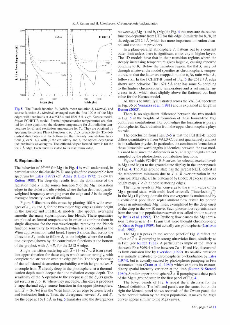
Fig. 5. The Planck function Bν (solid), mean radiation Jν (dotted), andsource function S ν (dashed) averaged over the first 100 Å of the Mg iedges with thresholds at λ= 2512.4 and 1621.5 Å. Left: Kurucz model.Right: FCHHT-B model. Formal representative temperatures are plot-ted for these quantities: the electron temperature for Bν, radiation tem-perature for Jν, and excitation temperature for S ν. They are obtained byapplying the inverse Planck function to Bν, Jν, S ν, respectively. The dot-dashed distributions at the bottom are the intensity contribution func-tions jν exp(−τν), with jν the emissivity and τν the optical depth,nearthe thresholds wavelengths. The lefthand deeper-formed curve is for the2512 Å edge. Each curve is scaled to its maximum value.

5. Explanation

The behavior of bZwaan1 for Mg i in Fig. 4 is well-understood, in

particular since the classic Ph.D. analysis of the comparable ironspectrum by Lites (1972) (cf. Athay & Lites 1972; review byRutten 1988). The deep dip results from the dominance of theradiation field J in the source function S of the Mg i ionizationedges in the violet and ultraviolet, where the bar denotes opacity-weighted frequency averaging over the edge and J is the angle-averaged intensity over all directions.

Figure 5 illustrates this cause by plotting 100 Å-wide aver-ages of S ν, Bν and Jν for the two major Mg i edges against heightin the Kurucz and FCHHT-B models. The spectral averagingsmooths the many superimposed line blends. These quantitiesare plotted as formal temperatures in order to combine them insingle diagrams for the two wavelengths, removing the Planckfunction sensitivity to wavelength (which is exponential in theWien approximation valid here). Figure 5 shows that across theultraviolet S ν tends to follow Jν at the heights where the radia-tion escapes (shown by the contribution functions at the bottomof the graphs), with Jν≈Bν for the 2512 Å edge.

Single-transition scattering with S = (1−ε) J+ε B is an excel-lent approximation for these edges which scatter strongly, withcomplete redistribution over the edge profile. The steep decreaseof the collisional destruction probability ε with height makes Suncouple from B already deep in the photosphere, at a thermal-ization depth much deeper than the radiation escape depth. Thesensitivity of the Λ operator to the steepness of the S ν(τ) gradi-ent results in Jν > Bν where they uncouple. This excess producesa superthermal edge source function in the upper photosphere,with S ≈ (bc/bi) B in the Wien limit for an edge between level iand ionization limit c. Thus, the divergence between S ν and Bνfor the edge at 1621.5 Å in Fig. 5 translates into the divergences

between bc (Mg ii) and b1 (Mg i) in Fig. 4 that measure the sourcefunction departure from LTE for this edge. Similarly for bc/b2 inthe edge at 2512.4 Å (which is a more important ionization chan-nel and continuum provider).

In a plane-parallel atmosphere Jν flattens out to a constantouter limit unless there is significant emissivity in higher layers.The 1D models have that in their transition regions where thesteeply increasing temperature gives larger ε, causing renewedcoupling to Bν. Below the transition region, the flat Jν may cutthrough whatever the model specifies as chromospheric temper-atures, so that the latter are mapped into the bc/bi ratio when S νfollows Jν. In the FCHHT-B panel of Fig. 5 the 2512.4 Å edgeshows such behavior. The 1621.5 Å edge has some S ν couplingto the higher chromospheric temperature and a yet smaller in-crease in Jν, which rises slightly above the flattened-out limitvalue for the Kurucz model.

All this is beautifully illustrated across the VAL3-C spectrumin Fig. 36 of Vernazza et al. (1981) and is explained at length inRutten (2003).

There is no significant difference between the two modelsin Fig. 5 at the heights of formation of these bound-free Mg icontinuum contributions. For both edges the formation is purelyphotospheric. Backradiation from the upper chromosphere playsno role.

The conclusion from Figs. 2–5 is that the FCHHT-B modeldiffers quantitatively from VAL3-C, but not qualitatively and notin its radiation physics. In particular, the continuum formation atthese ultraviolet wavelengths is identical between the two mod-els used here since the differences in S ν at larger heights are notsampled by the photospheric contribution functions.

Figure 6 adds FCHHT-B b curves for selected excited levelsin Mg i and Mg ii to the ground-state display in the upper panelsof Fig. 4. The Mg i ground state has the largest NLTE deficit inthe temperature minimum due to J > B overionization in theprincipal Mg i edges. The plateau of b1 (index 0) excess at largerheight maps J < B in these scattering edges.

The higher levels in Mg i converge to the b ≈ 1 value of theMg ii ground state, with multi-level crosstalk (“interlocking”).In the Mg i Rydberg domain this convergence is maintained bya collisional population replenishment flow driven by photonlosses in intermediate Mg i lines, exemplified by the deep onsetof the drop in the n= 10 curve. Such photon-loss replenishmentfrom the next-ion population reservoir was called photon suctionby Bruls et al. (1992). The Rydberg flow causes the Mg i emis-sion features near λ = 12μm that were thought chromosphericby Zirin & Popp (1989), but actually are photospheric (Carlssonet al. 1992).

The Mg ii b peaks in the second panel of Fig. 6 reflect theeffect of J > B pumping in strong ultraviolet lines, similarly asin Fe ii (see Rutten 1988). A particular example of the latter isthe weak Fe ii 3969.4 Å line between Ca ii H and Hε, discoveredas limb emission line by Evershed (1929). Its on-disk emissionwas initially attributed to chromospheric backradiation by Lites(1974), but is actually caused by photospheric pumping in Fe iiresonance lines (Cram et al. 1980) which explains its extraor-dinary spatial intensity variation at the limb (Rutten & Stencel1980). Similar upper-photosphere J > B pumping sets the b peakof the Mg iii ground state in the first panel of Fig. 4.

The lower panels of Fig. 6 repeat the b displays for theMenzel definition. The lefthand panels are the same, but on theright the Menzel panel shows reversals of the Zwaan panel dueto the normalization by the Mg iii population. It makes the Mg iicurves appear similar to the Mg i curves.

A86, page 5 of 11

A&A 540, A86 (2012)

Fig. 6. Population departures of selected magnesium levels in theFCHHT-B model. The level numbers increase with excitation energy.Left: Mg i. Right: Mg ii. Upper row: Zwaan definition. Lower row:Menzel definition.

The lower panels of Fig. 6 are similar to the correspondingMg i and Mg ii panels in Fig. 4 of Fontenla et al. (2009). Thelook-alike sequences of dips, deepest for the lowest levels, intheir six Menzel plots made Fontenla et al. (2009) conclude: “Allour results display overionization (i.e., ground-level departurefrom LTE coefficients smaller than unity) of all species aroundthe temperature minimum. [. . . ] Also, near the temperature min-imum the lower levels have smaller departure coefficients thanthe upper levels, indicating that the overionization of neutralsis a result from FUV and/or EUV irradiation which primarilyaffects lower levels. This indicates that overionization is muchmore affected by the irradiation from the upper chromospherein continuum and emission lines than by the photospheric ra-diation and absorption lines. Therefore, we stress that the con-sideration of a realistic upper chromosphere is essential to thedetermination of the densities near the temperature minimum of(1) neutral low first-ionization-potential (FIP) elements, and (2)singly ionized high FIP elements. Even a very sophisticated cal-culation of the effects of lower chromospheric absorption lineson the elemental ionization can produce unrealistic results if itdoes not include upper chromosphere irradiation”. This inter-pretation is incorrect. Downward irradiation does not affect thedegree of ionization of these minority species around the temper-ature minimum of the FCHHT-B model. We have demonstratedthis for Mg here; the same applies to Fe, Si, Al.

However, more positively, we wish to note that the model-ing of Fontenla et al. (2009) is not impaired by this misinter-pretation of its results, and that that does not detract value fromtheir effort. In this era of giant computer programs it becomesnon-trivial to diagnose what the output implies. Chromosphericphysics is becoming a key area in solar research but does requireunderstanding of complex non-equilibrium optically-thick spec-trum formation. Our tutorial elucidation of this particular issuemay be instructive to newcomers to the field.

Fig. 7. Hα formation for the Kurucz (left) and FCHHT-B (right) mod-els. Solid: Planck function Bν at line center. Dashed: angle-averaged ra-diation Jν at line center. Dotted: total source function S ν at line center.The ticks mark the locations with line-center optical depth τν = 3, 1, 0.3from left to right.

6. Backradiation in Hα

Figure 7 shows formation parameters for Hα in the Kurucz andFCHHT-B models. It is similar to Fig. 8 in Cauzzi et al. (2009),but here, prompted by the referee and in the vein of this paper,we add detailed analysis using the FCHHT-B model for demon-stration. We do not regard it a viable explanation of actual solarHα formation (Sect. 7), but use it rather as a one-dimensionaldidactic “FCHHT-B star”.

The lefthand panel of Fig. 7 illustrates Hα line formationin such a star without overlying chromosphere. At line center,Jν drops well below Bν. This behavior differs from the Jν > Bνexcesses of the ultraviolet continua in Fig. 5 because the Planck-function sensitivity to temperature is smaller at longer wave-lengths, flattening the dBν/dh gradient, and because the substan-tial additional line opacity αl

ν flattens the dBν/dτν = dBν/[(αcν +

αlν) dz] gradient yet more. The Λ operator then produces Jν < S ν

tending toward the S ν(0) =√ενBν surface value for a scattering

isothermal atmosphere with constant εν.In the Kurucz model the Hα core originates from the upper

photosphere around h = 400 km as a deep, strongly scatteringline with S ν ≈ Jν0 . The corresponding emergent profile is shownin the top panel of Fig. 8. It is well reproduced by applying theEddington-Barbier approximation Iν ≈ S ν(τν=1).

The righthand panel of Fig. 7 shows the formation of Hαin the FCHHT-B model. Its chromospheric high-temperatureplateau supplies sufficient Hα opacity that at line center τν=1 isreached about a thousand km higher than in the Kurucz model.The line-center formation is again well described by Iν ≈ S ν(τν=1) ≈ Jν0 (τν=1), but the Eddington-Barbier approximation is lesswell applicable in the line wings which have a formation gapbetween photosphere and chromosphere (e.g., Schoolman 1972;Leenaarts et al. 2006). This gap is detailed in Fig. 9 which showsHα opacities and optical depth scales, with the opacities multi-plied by the scale height in the upper FCHHT-B photosphere (itdoubles in the FCHHT-B chromosphere from a steep increase ofthe imposed non-gravitational acceleration). The line extinctionhas a deep dip in the temperature minimum. Correspondingly,the optical depth buildup (dotted curves) levels out. At line cen-ter the FCHHT-B chromosphere has optical thickness τν = 3.5.At Δλ = −0.44 Å τν = 0.3 (outer tick) is reached already in thechromosphere but τν = 1 only a thousand km deeper in the pho-tosphere. At Δλ = −0.74 Å the FCHHT-B chromosphere is vir-tually transparent.

A86, page 6 of 11

R. J. Rutten and H. Uitenbroek: Chromospheric backradiation

Fig. 8. Top panel: emergent Hα intensity profiles at disk center com-puted from the FCHHT-B (dotted) and Kurucz (dashed) models, incomparison with the observed spatially-averaged profile (solid) takenfrom the atlas observed by Brault & Testerman, calibrated by Neckel& Labs (1984), and posted by Neckel (1999). Lower panels: mean in-tensity Jν across Hα at different heights in the Kurucz and FCHHT-Batmospheres, respectively. For the Kurucz panel the sampling heightsare 26, 41, 157, 283, 358 and 995 km. For the FCHHT-B panel they are35, 150, 300, 519, 850, 1000, 1340 and 1701 km. The dotted profile inthe bottom panel is the outward intensity at height 850 km, impingingon the FCHHT-B chromosphere. The dotted profile in the middle panelis the outward intensity at height 252 km in the Kurucz model wherethe line-center optical depth equals the optical thickness τν = 3.5 of theFCHHT-B chromosphere.

At line center the line extinction much exceeds the continu-ous extinction even in the dip, so that the total source functionequals the line source function at all heights. In the wings theline extinction drops below the continuum extinction. Where thishappens the total source function drops to the Planck function(not shown).

Figure 10 shows the departure coefficients b2 and b3 (Zwaandefinition) governing Hα in the FCHHT-B model. The curve di-vergence log(b3) − log(b2) corresponds to the curve divergencelog(S ν) − log(Bν) in the FCHHT-B panel of Fig. 7. Throughoutthe near-isothermal FCHHT-B chromosphere the Hα opacity isnearly in LTE because the formation of Lyα is close to detailedbalancing there. However, this is not the case in the deep tem-perature minimum and steep rise to the chromospheric tempera-ture. Here theΛ operator smooths the rapid temperature changesfor the scattering-dominated Lyα source function (not shown)

Fig. 9. Solid: Hα line extinction coefficients αlν per m against height for

the FCHHT-B model, at line center and in the blue wing at Δλ=−0.44and −0.74 Å, and the continuous opacity αc

ν in the adjacent continuum.The dot-dashed curve is the line-center result for LTE. The opacitiesare multiplied by a scale height of 105 m to make them comparable tothe corresponding optical depth scales (dotted curves). The tick markson the latter correspond to τν = 3, 1, 0.3. Across the opacity dip due tothe temperature minimum the optical depth is τν = 3.5, 0.7, 0.04 at thethree line wavelengths, respectively.

Fig. 10. Hα population departure coefficients against height for theFCHHT-B model. The tick marks correspond to τν = 3, 1, 0.3. Solid:lower-level departure coefficient b2. Dashed: upper-level departure co-efficient b3.

which has S ν ≈ Jν ≈ b2 Bν. This Lyα smoothing causes the highpeak in b2 and considerable corresponding fill-in of the opacitydips in Fig. 9, illustrated for line center as difference with themuch deeper dot-dashed LTE curve. In this manner Lyα scat-tering compensates for low-temperature Hα opacity loss whencool features are narrow in spatial extent. The b2 peak in Fig. 10doubles if CRD is adopted for Lyα, from additional smoothingthrough farther wing-photon travel.

The corresponding emergent intensity profile in the top panelof Fig. 8 is similar to the Kurucz result despite the disparate lineformation. Both are reasonably good approximations to the ob-served mean quiet-Sun profile. Both gain fit quality in the wingsif the computed continuum intensity is rescaled to the observedvalue. Increase of the microturbulence in the Kurucz model from1.5 to about 10 km s−1 produces a good core fit for this model aswell.

The Jν curves in Fig. 7 show that the opacity gap in theFCHHT-B model contains much more Hα radiation than atcorresponding heights in the Kurucz model. This Hα radia-tion fill-in causes a yet higher peak for b3 in Fig. 10. It is de-tailed in the lower panels of Fig. 8. In the lower photospherethe Hα Jν profiles are the same for the two models, but above

A86, page 7 of 11

A&A 540, A86 (2012)

h ≈ 250 km the Kurucz model gives absorption cores whereasthe FCHHT-B model predicts slightly self-reversed cores acrossthe opacity gap. This difference explains that for the Kuruczmodel Jν0 (shown by the line-center S ν curve in the lefthandpanel of Fig. 7) ends up higher than Jν at line center, whereasfor the FCHHT-B model S ν ≈ Jν0 coincides with line-centerJν across the opacity gap in the righthand panel of Fig. 7. Thelarge core width of the highest-formed FCHHT-B profiles comesfrom large thermal broadening (about 10 km s−1) and yet largermicroturbulence (about 15 km s−1).

Because the FCHHT-B chromosphere is near-isothermal theHα formation is comparable to the classic results for a finiteisothermal scattering atmosphere of Avrett & Hummer (1965),in particular their optically thick but effectively thin case inwhich the line source function does not reach thermalization.The main difference is that the FCHHT-B chromosphere is ir-radiated from below. The impinging intensity profile in the out-ward direction is shown by the dotted curve in the bottom panelof Fig. 8. This line is much shallower than the emergent pro-file from the Kurucz model, in agreement with the much higherJν above h ≈ 200 km. A test with a hotter chromosphere, i.e.,thicker in Hα, gives more backradiation and a higher imping-ing profile with a bright self-reversed core. However, the deepemergent-intensity core remains about the same.

Thus, the presence of an opaque chromosphere changes theillumination profile with respect to the profile that emerges fromthe same photosphere without overlying chromosphere. A math-ematical explanation is given by the principle of invariance(p. 165 of Chandrasekhar 1950) regarding addition or subtrac-tion of a layer of arbitrary optical thickness to a semi-infiniteplane-parallel atmosphere; creating a gap or pushing down thefinite chromospheric atmosphere over the gap to where it meetssimilar source conditions does not change the emergent radia-tion. A more physical explanation is that the radiation field inthe gap builds up due to backradiation from the overlying chro-mosphere (called reflection by Chandrasekhar 1950).

We now demonstrate that this backradiation is dominated bytwo-level scattering. The line source function for complete re-distribution can be written as:

S lν0= (1 − εν0 − ην0 ) Jν0 + εν0 Bν0(T ) + ην0 Bν0(Td) (4)

=Jν0 + ε

′ν0

Bν0(T ) + η′ν0 Bν0(Td)

1 + ε′ν0 + η′ν0

, (5)

where Jν0 is the profile-averaged mean intensity, εν0 the thermaldestruction probability, i.e., the fraction of line-photon extinc-tions by direct collisional deexcitation corrected for emissivityfrom spontaneous scattering, ην0 the fractional probability of allindirect detour extinction, with detour meaning any multi-levelpath from the upper to the lower level not including the directtransition, corrected for stimulated detour emissivity, and ε′ν0 andη′ν0 the corresponding ratios of such extinctions to the contribu-tion by two-level scattering. The formal detour excitation tem-perature Td is given by (gu Dul)/(gl Dlu) ≡ exp(hν0/kTd) whereDul is the summed transition probability (per second per parti-cle in the upper level) of all detour upper-to-lower paths, Dlu forall detour lower-to-upper paths, and gl and gu are the statisticalweights.

The classic literature used Eq. (5) (e.g., Gebbie & Steinitz1974; Sect. 8.1 of Jefferies 1968; Eq. (12.11) of Mihalas 1970)following Thomas (1957) who divided strong lines into “colli-sion type” with εν0 > ην0 and “photoelectric type” with ην0 > εν0 ,designating Hα as principal example of the second type. In par-ticular, Hα would gain most photons from Balmer ionization

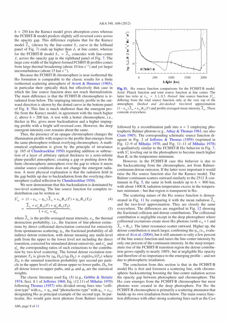
Fig. 11. Hα source function comparisons for the FCHHT-B model.Solid: Planck function and total source function at line center. Thelatter has ticks at τν0 = 3, 1, 0.3. Dotted: line source function S l

ν0,

differing from the total source function only at the very top of theatmosphere. Dashed and dot-dashed: two-level approximation(1− εν0 ) Jν0 + εν0 Bν0 (T ) and profile-averaged mean intensity Jν0 . Thesecoincide everywhere.

followed by a recombination path into n = 3 employing pho-tospheric Balmer photons (e.g., Athay & Thomas 1961; see alsoCram 1985). The corresponding schematic source function di-agram in Fig. 3 of Jefferies & Thomas (1959) (reprinted inFig. 12–9 of Mihalas 1970, and Fig. 11–11 of Mihalas 1978)is qualitatively similar to the FCHHT-B Hα behavior in Fig. 7,with S l

ν leveling out in the photosphere to become much higherthan Bν in the temperature minimum.

However, in the FCHHT-B case this behavior is due tothe backscattering from the chromosphere, not from Balmer-continuum detour emission. If the latter were important it wouldraise the Hα source function also for the Kurucz model. TheBalmer continuum scatters outward similarly to the 2512 Å con-tinuum in Fig. 5, the same in both models up to h ≈ 800 km,with about 1400 K radiation temperature excess in the tempera-ture minimum – but that region is transparent in Hα.

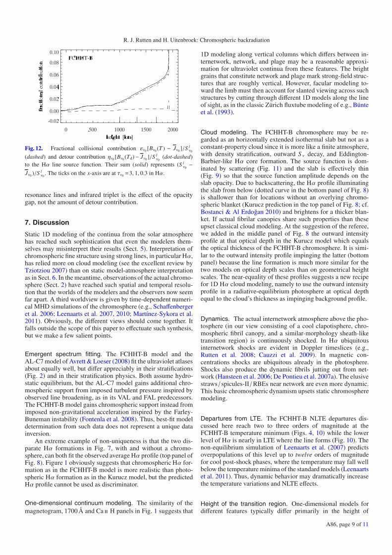
The scattering nature of the Hα source function is demon-strated in Fig. 11 by comparing it with the mean radiation Jν0and the two-level approximation. They are closely the sameeverywhere. The differences are magnified in Fig. 12 showingthe fractional collision and detour contributions. The collisionalcontribution is negligible except in the deep photosphere wherecollisional excitations create most Hα photons (with εν0 ≈1 andJν0 ≈ Bν0). The latter resonance-scatter outward. Higher up, thedetour contribution is much larger, confirming the ην0/εν0 evalu-ation of Al et al. (2004), but it still amounts to only a few percentof the line source function and raises the line-center intensity byonly one percent of the continuum intensity. In the steep temper-ature rise of the FCHHT-B transition region the detour contribu-tion grows rapidly to nearly 100%, but at negligible Hα opacityand therefore of no importance to the emerging profile – and notdue to photospheric irradiation.

The conclusion from this section is that in the FCHHT-Bmodel Hα is first and foremost a scattering line, with chromo-spheric backscattering boosting the line-center radiation acrossthe opacity gap between photosphere and chromosphere. TheHα core emerges from the FCHHT-B chromosphere but mostphotons were created in the deep photosphere. For Hα theFCHHT-B chromosphere is primarily a scattering attenuator thatbuilds up its own irradiation from below. The main source func-tion difference with other strong scattering lines such as the Ca ii

A86, page 8 of 11

R. J. Rutten and H. Uitenbroek: Chromospheric backradiation

Fig. 12. Fractional collisional contribution εν0 [Bν0 (T ) − Jν0 ]/S lν0

(dashed) and detour contribution ην0 [Bν0(Td)− Jν0 ]/S lν0

(dot-dashed)to the Hα line source function. Their sum (solid) represents (S l

ν0−

Jν0 )/S lν0

. The ticks on the x-axis are at τν0 =3, 1, 0.3 in Hα.

resonance lines and infrared triplet is the effect of the opacitygap, not the amount of detour contribution.

7. Discussion

Static 1D modeling of the continua from the solar atmospherehas reached such sophistication that even the modelers them-selves may misinterpret their results (Sect. 5). Interpretation ofchromospheric fine structure using strong lines, in particular Hα,has relied more on cloud modeling (see the excellent review byTziotziou 2007) than on static model-atmosphere interpretationas in Sect. 6. In the meantime, observations of the actual chromo-sphere (Sect. 2) have reached such spatial and temporal resolu-tion that the worlds of the modelers and the observers now seemfar apart. A third worldview is given by time-dependent numeri-cal MHD simulations of the chromosphere (e.g., Schaffenbergeret al. 2006; Leenaarts et al. 2007, 2010; Martínez-Sykora et al.2011). Obviously, the different views should come together. Itfalls outside the scope of this paper to effectuate such synthesis,but we make a few salient points.

Emergent spectrum fitting. The FCHHT-B model and theAL-C7 model of Avrett & Loeser (2008) fit the ultraviolet atlasesabout equally well, but differ appreciably in their stratifications(Fig. 2) and in their stratification physics. Both assume hydro-static equilibrium, but the AL-C7 model gains additional chro-mospheric support from imposed turbulent pressure inspired byobserved line broadening, as in its VAL and FAL predecessors.The FCHHT-B model gains chromospheric support instead fromimposed non-gravitational acceleration inspired by the Farley-Buneman instability (Fontenla et al. 2008). Thus, best-fit modeldetermination from such data does not represent a unique datainversion.

An extreme example of non-uniqueness is that the two dis-parate Hα formations in Fig. 7, with and without a chromo-sphere, can both fit the observed average Hα profile (top panel ofFig. 8). Figure 1 obviously suggests that chromospheric Hα for-mation as in the FCHHT-B model is more realistic than photo-spheric Hα formation as in the Kurucz model, but the predictedHα profile cannot be used as discriminator.

One-dimensional continuum modeling. The similarity of themagnetogram, 1700 Å and Ca ii H panels in Fig. 1 suggests that

1D modeling along vertical columns which differs between in-ternetwork, network, and plage may be a reasonable approxi-mation for ultraviolet continua from these features. The brightgrains that constitute network and plage mark strong-field struc-tures that are roughly vertical. However, facular modeling to-ward the limb must then account for slanted viewing across suchstructures by cutting through different 1D models along the lineof sight, as in the classic Zürich fluxtube modeling of e.g., Bünteet al. (1993).

Cloud modeling. The FCHHT-B chromosphere may be re-garded as an horizontally extended isothermal slab but not as aconstant-property cloud since it is more like a finite atmosphere,with density stratification, outward S ν decay, and Eddington-Barbier-like Hα core formation. The source function is dom-inated by scattering (Fig. 11) and the slab is effectively thin(Fig. 9) so that the source function amplitude depends on theslab opacity. Due to backscattering, the Hα profile illuminatingthe slab from below (dotted curve in the bottom panel of Fig. 8)is shallower than for locations without an overlying chromo-spheric blanket (Kurucz prediction in the top panel of Fig. 8; cf.Bostanci & Al Erdogan 2010) and brightens for a thicker blan-ket. If actual fibrilar canopies share such properties than theseupset classical cloud modeling. At the suggestion of the referee,we added in the middle panel of Fig. 8 the outward intensityprofile at that optical depth in the Kurucz model which equalsthe optical thickness of the FCHHT-B chromosphere. It is simi-lar to the outward intensity profile impinging the latter (bottompanel) because the line formation is much more similar for thetwo models on optical depth scales than on geometrical heightscales. The near-equality of these profiles suggests a new recipefor 1D Hα cloud modeling, namely to use the outward intensityprofile in a radiative-equilibrium photosphere at optical depthequal to the cloud’s thickness as impinging background profile.

Dynamics. The actual internetwork atmosphere above the pho-tosphere (in our view consisting of a cool clapotisphere, chro-mospheric fibril canopy, and a similar-morphology sheath-liketransition region) is continuously shocked. In Hα ubiquitousinternetwork shocks are evident in Doppler timeslices (e.g.,Rutten et al. 2008; Cauzzi et al. 2009). In magnetic con-centrations shocks are ubiquitous already in the photosphere.Shocks also produce the dynamic fibrils jutting out from net-work (Hansteen et al. 2006; De Pontieu et al. 2007a). The elusivestraws / spicules-II /RBEs near network are even more dynamic.This basic chromospheric dynamism upsets static chromospheremodeling.

Departures from LTE. The FCHHT-B NLTE departures dis-cussed here reach two to three orders of magnitude at theFCHHT-B temperature minimum (Figs. 4, 10) while the lowerlevel of Hα is nearly in LTE where the line forms (Fig. 10). Thenon-equilibrium simulation of Leenaarts et al. (2007) predictsoverpopulations of this level up to twelve orders of magnitudefor cool post-shock phases, where the temperature may fall wellbelow the temperature minima of the standard models (Leenaartset al. 2011). Thus, dynamic behavior may dramatically increasethe temperature variations and NLTE effects.

Height of the transition region. One-dimensional models fordifferent features typically differ primarily in the height of

A86, page 9 of 11

A&A 540, A86 (2012)

their transition region. Simulations as the one of Leenaartset al. (2007) suggest that the transition region above inter-network is kicked up and mass-loaded by field-guided flowsthat do not obey one-dimensional hydrostatic equilibrium. Inthis simulation the location of the transition region varies overh = 1000−4000 km, with rapid changes, and is generally lowerabove magnetic concentrations. Such larger range than in the 1Dmodel grids may better reflect actual variations in fibril-canopyheight or corrugation.

Hα opacity gap. The Hα opacity gap and backscattering intoit are properties of the FCHHT-B model. Do they also occur inthe real Sun? The images in Fig. 1 roughly agree with FCHHT-Bpredictions: in the 1700 Å image no fibrils are seen whereas theyappear opaque in the Hα image. Also, when one samples thereal Sun in Hα away from line center (e.g., in DOT movies2) thephotospheric granulation appears when the fibrils become trans-parent, without an intermediate clapotispheric scene as in theCa ii H and 1700 Å images in Fig. 1. Thus, a similar opacity gapseems to exist under the actual fibrilar canopies making up theinternetwork chromosphere. The radiation crossing it, boostedby backscattering, will suffer substantial spatial smoothing ofthe photospheric scene. Some of it may leak out through an ef-fectively thin fibril canopy, scatter around dark fibrils in photonchanneling as suggested by Al et al. (2004), or be seen fromaside as in the backradiation explanation of bright rims underfilaments (e.g., Kostik & Orlova 1975; cf. Panasenco 2010).

Hα detour brightening. In the FCHHT-B model Hα is an al-most pure scattering line (Fig. 11). The detour contributionην0 (Bν0(Td) − Jν0 ) to the line source function becomes impor-tant only in the transparent transition region (Fig. 12). In thereal Sun locations with very bright Hα, such as the moss andactive-region heart in Fig. 13 of Rutten (2007), may representlow-lying, denser transition regions that radiate Hα through re-combination paths.

8. Conclusion

The development of standard models of the solar atmosphere,masterminded by Avrett, represents a well-established pinna-cle of sophistication with respect to the application of NLTEspectrum formation theory with the inclusion of numerous spec-tral features. However, the assumption of hydrostatic and time-independent equilibria without magnetism remains a far cryfrom the actual solar chromosphere, which is pervaded byshocks and rapidly changing magnetic fine structure in even thequietest regions.

Conversely, state-of-the-art magnetohydrodynamics simula-tions do a good job in emulating the small-scale magnetody-namism of the actual solar atmosphere, but they remain weakin properly treating non-equilibrium radiation. Implementationof the art of the 1D modelers into the 3D time-dependent codesof the simulators presents a formidable challenge, but seems themost promising venue to understand the enigmatic solar chro-mosphere (cf. Leenaarts et al. 2012).

Acknowledgements. We thank E. Romashets, A. Sukhorukov and P. Sütterlinand the SDO team for their contributions to Fig. 1, H. Wang for discussing brightfilament rims, and J. Fontenla and the referee for pointing out severe shortcom-ings in earlier versions. This work was started at the Lockheed-Martin Solar

2 http://www.staff.science.uu.nl/~rutte101/dot

and Astrophysics Laboratory when both authors were visiting, RJR supportedby NASA contracts NNG09FA40C (IRIS) and NNM07AA01C (HINODE). Ourresearch made much use of NASA’s Astrophysics Data System.

ReferencesAl, N., Bendlin, C., Hirzberger, J., Kneer, F., & Trujillo Bueno, J. 2004, A&A,

418, 1131Athay, R. G., & Thomas, R. N. 1961, Physics of the solar chromosphere

(New York: Interscience)Athay, R. G., & Lites, B. W. 1972, ApJ, 176, 809Avrett, E. H., & Hummer, D. G. 1965, MNRAS, 130, 295Avrett, E. H., & Loeser, R. 2008, ApJS, 175, 229Bostanci, Z. F., & Al Erdogan, N. 2010, MemSAI, 81, 769Bray, R. J., & Loughhead, R. E. 1974, The solar chromosphere (London:

Chapman & Hall)Brekke, P. 1993, ApJS, 87, 443Bruls, J. H. M. J., Rutten, R. J., & Shchukina, N. G. 1992, A&A, 265, 237Bünte, M., Solanki, S. K., & Steiner, O. 1993, A&A, 268, 736Carlsson, M., & Stein, R. F. 1995, ApJ, 440, L29Carlsson, M., & Stein, R. F. 1997, ApJ, 481, 500Carlsson, M., Rutten, R. J., & Shchukina, N. G. 1992, A&A, 253, 567Carlsson, M., Hansteen, V. H., & Gudiksen, B. V. 2010, MemSAI, 81, 582Cauzzi, G., Reardon, K., Rutten, R. J., Tritschler, A., & Uitenbroek, H. 2009,

A&A, 503, 577Chandrasekhar, S. 1950, Radiative transfer (Oxford: Clarendon)Cram, L. E. 1985, in Chromospheric diagnostics and modelling, ed. B. W. Lites,

Procs. NSO Summer Conf., 288Cram, L. E., Lites, B. W., & Rutten, R. J. 1980, ApJ, 241, 374Curdt, W., Brekke, P., Feldman, U., et al. 2001, A&A, 375, 591de Jager, C. 1959, Handbuch der Physik, 52, 80De Pontieu, B., Hansteen, V. H., Rouppe van der Voort, L., van Noort, M., &

Carlsson, M. 2007a, ApJ, 655, 624De Pontieu, B., McIntosh, S., Hansteen, V. H., et al. 2007b, PASJ, 59, 655Evershed, J. 1929, MNRAS, 89, 566Fontenla, J. M., Avrett, E. H., & Loeser, R. 1990, ApJ, 355, 700Fontenla, J. M., Avrett, E. H., & Loeser, R. 1991, ApJ, 377, 712Fontenla, J. M., Avrett, E. H., & Loeser, R. 1993, ApJ, 406, 319Fontenla, J. M., Avrett, E. H., & Loeser, R. 2002, ApJ, 572, 636Fontenla, J. M., Avrett, E., Thuillier, G., & Harder, J. 2006, ApJ, 639, 441Fontenla, J. M., Balasubramaniam, K. S., & Harder, J. 2007, ApJ, 667, 1243Fontenla, J. M., Peterson, W. K., & Harder, J. 2008, A&A, 480, 839Fontenla, J. M., Curdt, W., Haberreiter, M., Harder, J., & Tian, H. 2009, ApJ,

707, 482Gebbie, K. B., & Steinitz, R. 1974, ApJ, 188, 399Gingerich, O., & de Jager, C. 1968, Sol. Phys., 3, 5Gingerich, O., Noyes, R. W., Kalkofen, W., & Cuny, Y. 1971, Sol. Phys., 18, 347Greve, A., & Zwaan, C. 1980, A&A, 90, 239Gustafsson, B., Bell, R. A., Eriksson, K., & Nordlund, A. 1975, A&A, 42, 407Gustafsson, B., Edvardsson, B., Eriksson, K., et al. 2008, A&A, 486, 951Hansteen, V. H., De Pontieu, B., Rouppe van der Voort, L., van Noort, M., &

Carlsson, M. 2006, ApJ, 647, L73Heintze, J. R. W., Hubenet, H., & de Jager, C. 1964a, Bull. Astr. Inst. Neth., 17,

442Heintze, J. R. W., Hubenet, H., & de Jager, C. 1964b, SAO Special Report, 167,

240Heinzel, P., & Schmieder, B. 1994, A&A, 282, 939Holweger, H. 1967, Z. Astrophys., 65, 365Holweger, H., & Müller, E. A. 1974, Sol. Phys., 39, 19Jefferies, J. T. 1968, Spectral line formation (Waltham: Blaisdell)Jefferies, J. T., & Thomas, R. N. 1959, ApJ, 129, 401Judge, P. G., Tritschler, A., & Chye Low, B. 2011, ApJ, 730, L4Kostik, R. I., & Orlova, T. V. 1975, Sol. Phys., 45, 119Koza, J., Rutten, R. J., & Vourlidas, A. 2009, A&A, 499, 917Kurucz, R. L. 1974, Sol. Phys., 34, 17Kurucz, R. L. 1979, ApJS, 40, 1Kurucz, R. L. 1992a, Rev. Mex. Astron. Astrofis., 23, 181Kurucz, R. L. 1992b, Rev. Mex. Astron. Astrofis., 23, 187Kurucz, R. L. 1994, Solar abundance model atmospheres, CD-ROM 19, SAO,

Cambridge, Mass.Leenaarts, J., Rutten, R. J., Sütterlin, P., Carlsson, M., & Uitenbroek, H. 2006,

A&A, 449, 1209Leenaarts, J., Carlsson, M., Hansteen, V., & Rutten, R. J. 2007, A&A, 473, 625Leenaarts, J., Rutten, R. J., Reardon, K., Carlsson, M., & Hansteen, V. 2010,

ApJ, 709, 1362Leenaarts, J., Carlsson, M., Hansteen, V., & Gudiksen, B. V. 2011, A&A, 530,

A124

A86, page 10 of 11

R. J. Rutten and H. Uitenbroek: Chromospheric backradiation

Leenaarts, J., Carlsson, M., & Rouppe van der Voort, L. 2012, ApJ, in press[arXiv:1202.1926]

Lites, B. W. 1972, Ph.D. Thesis, Univ. Colorado, BoulderLites, B. W. 1974, A&A, 33, 363Lockyer, J. N. 1868, Roy. Soc. London Procs. Ser. I, 17, 131Maltby, P., Avrett, E. H., Carlsson, M., et al. 1986, ApJ, 306, 284Martínez-Sykora, J., Hansteen, V., & Moreno-Insertis, F. 2011, ApJ, 736, 9Menzel, D. H., & Cillié, G. G. 1937, ApJ, 85, 88Mihalas, D. 1970, Stellar atmospheres (San Francisco: Freeman)Mihalas, D. 1978, Stellar atmospheres, 2nd edn. (San Francisco: Freeman)Neckel, H. 1999, Sol. Phys., 184, 421Neckel, H., & Labs, D. 1984, Sol. Phys., 90, 205Panasenco, O. 2010, MemSAI, 81, 673Reardon, K. P., Uitenbroek, H., & Cauzzi, G. 2009, A&A, 500, 1239Rouppe van der Voort, L. H. M., De Pontieu, B., Hansteen, V. H., Carlsson, M.,

& van Noort, M. 2007, ApJ, 660, L169Rouppe van der Voort, L., Leenaarts, J., De Pontieu, B., Carlsson, M., & Vissers,

G. 2009, ApJ, 705, 272Rutten, R. J. 1988, in Physics of formation of Fe II lines outside LTE, ed.

R. Viotti, A. Vittone, & M. Friedjung, ASSL, 138, IAU Colloq., 94, 185Rutten, R. J. 1995, in Helioseismology, ESA-SP, 376, 151Rutten, R. J. 2003, Radiative transfer in stellar atmospheres, Lecture Notes,

Utrecht UniversityRutten, R. J. 2006, in Solar MHD Theory and Observations: A High Spatial

Resolution Perspective, ed. J. Leibacher, R. F. Stein, & H. Uitenbroek, ASPConf. Ser., 354, 276

Rutten, R. J. 2007, in The physics of chromospheric plasmas, ed. P. Heinzel,I. Dorotovic, & R. J. Rutten, ASP Conf. Ser., 368, 27

Rutten, R. J. 2012, Phil. Trans. R. Soc. A, in press [arXiv:1110.6606]Rutten, R. J., & Stencel, R. E. 1980, A&AS, 39, 415Rutten, R. J., & Uitenbroek, H. 1991, Sol. Phys., 134, 15Rutten, R. J., van Veelen, B., & Sütterlin, P. 2008, Sol. Phys., 251, 533Rutten, R. J., Leenaarts, J., Rouppe van der Voort, L. H. M., et al. 2011, A&A,

531, A17Rybicki, G. B., & Hummer, D. G. 1991, A&A, 245, 171Rybicki, G. B., & Hummer, D. G. 1992, A&A, 262, 209Schaffenberger, W., Wedemeyer-Böhm, S., Steiner, O., & Freytag, B. 2006, in

Solar MHD Theory and Observations: A High Spatial Resolution Perspective,ed. J. Leibacher, R. F. Stein, & H. Uitenbroek, ASP Conf. Ser., 354, 345

Schoolman, S. A. 1972, Sol. Phys., 22, 344Steiner, O., Grossmann-Doerth, U., Knölker, M., & Schüssler, M. 1998, ApJ,

495, 468Thomas, R. N. 1957, ApJ, 125, 260Tziotziou, K. 2007, in The physics of chromospheric plasmas, ed. P. Heinzel,

I. Dorotovic, & R. J. Rutten, ASP Conf. Ser., 368, 217Uitenbroek, H. 1997, Sol. Phys., 172, 109Uitenbroek, H. 2001, ApJ, 557, 389van Regemorter, H. 1962, ApJ, 136, 906Vernazza, J. E., Avrett, E. H., & Loeser, R. 1973, ApJ, 184, 605Vernazza, J. E., Avrett, E. H., & Loeser, R. 1976, ApJS, 30, 1Vernazza, J. E., Avrett, E. H., & Loeser, R. 1981, ApJS, 45, 635Vourlidas, A., Sánchez Andrade-Nuño, B., Landi, E., et al. 2010, Sol. Phys., 261,

53Wijbenga, J. W., & Zwaan, C. 1972, Sol. Phys., 23, 265Zirin, H., & Popp, B. 1989, ApJ, 340, 571

A86, page 11 of 11