Astronomy

ASTRONOMICALOBSERVATION

HANDBOOK

ASTRONOMICAL OBSERVATIONS

-i-

Astronomical Observation HandbookCharles D. Ghilani, Ph.D.

The Pennsylvania State University

Copyright © 1996 – 2004 by Charles D. Ghilani

All rights reservedReproduction or translation of any part of this work beyond that permitted by the United States Copyright Actwithout the permission of the copyright owner is unlawful. Requests for permission or further information shouldbe addressed to the author.

ASTRONOMICAL OBSERVATIONS

-ii-

TABLE OF CONTENTS

WHY MAKE ASTRONOMICAL OBSERVATIONS FOR AZIMUTH . . . . . . . . . . . . . . . . . . . . . . . . . . . . . . . . . 1

JUST WHICH NORTH ARE YOU TALKING ABOUT? . . . . . . . . . . . . . . . . . . . . . . . . . . . . . . . . . . . . . . . . . . . . 1

HISTORICAL METHODS OF DETERMINING AZIMUTH . . . . . . . . . . . . . . . . . . . . . . . . . . . . . . . . . . . . . . . . . 1

ACCURATE METHODS OF AZIMUTH DETERMINATION . . . . . . . . . . . . . . . . . . . . . . . . . . . . . . . . . . . . . . . . 2

BASIC DEFINITIONS . . . . . . . . . . . . . . . . . . . . . . . . . . . . . . . . . . . . . . . . . . . . . . . . . . . . . . . . . . . . . . . . . . . . . . . 3

SPHERICAL TRIGONOMETRIC FORMU LAS . . . . . . . . . . . . . . . . . . . . . . . . . . . . . . . . . . . . . . . . . . . . . . . . . . . 3

DERIVATION OF HOUR-ANGLE FORM ULA . . . . . . . . . . . . . . . . . . . . . . . . . . . . . . . . . . . . . . . . . . . . . . . . . . . 4

SPECIAL EQUIPMENT . . . . . . . . . . . . . . . . . . . . . . . . . . . . . . . . . . . . . . . . . . . . . . . . . . . . . . . . . . . . . . . . . . . . . . 5

WHAT’S IN A CELESTIAL OBSERVATION? . . . . . . . . . . . . . . . . . . . . . . . . . . . . . . . . . . . . . . . . . . . . . . . . . . . 6

METHODS OF OBSERVING A CELESTIAL OBJECT FOR AZIMUTH . . . . . . . . . . . . . . . . . . . . . . . . 6

Universal Coordinated Time (7)

Observing a Star (7)

Observing the Sun (7)

Field Procedures (8)

REDUCING CELESTIAL OBSERVATIONS FOR AZIMUTH . . . . . . . . . . . . . . . . . . . . . . . . . . . . . . . . 9

Declination. (9)

Greenwich Hour Angle (GHA) and the Local Hour Angle (LHA) (9)

Reduction Sheets (10)

SAMPLE COMPUTATIONS . . . . . . . . . . . . . . . . . . . . . . . . . . . . . . . . . . . . . . . . . . . . . . . . . . . . . . . . . . 11

Computations Using Software (12)

ERRORS IN CELESTIAL OBSERVATIONS . . . . . . . . . . . . . . . . . . . . . . . . . . . . . . . . . . . . . . . . . . . . . . . . . . . . 13

ASTRONOMICAL OBSERVATIONS FOR AZIMUTH 1

Figure 2 Shadow method.

1. WHY M AKE ASTRO NOM ICAL OBSERVATIONS FO R AZIMUTH

In a retracement survey, the land surveyor adheres to the fundamental principle of “following the footsteps of the original

surveyor”. Often, however, when creating a new subdivision of land, the surveyor fails to provide the measurement that

perpetuate their own work. While most surveyors will monument corners with artificial monuments, few will establish

any kind of recoverab le spatial orientation for the lines. It is not uncommon for surveyors to use adjoining property lines

for the bearing basis on the plot. Thus while the accuracy o f distance and angle measurements has increased, the

directions of lines may still be based on compass readings from the 19'th century. How many deeds exist today where

the bearings of the lines disagree? How many deeds have lines based on a composite of several adjoiners? How many

deeds have their directional orientation based on a single record line?

In fact, the record evidence for these lines is continually being lost due to the natural disappearance of monuments

caused by erosion, corrosion, and man-made events. Thus when the monuments of the lines become lost, they themselves

become unrecoverable. In fact, a surveyor who finds only a single monument in a property survey is confronted with the

problem of trying to establish the spatial orientation (bearing basis) for the property. Astronomical observations for

azimuth not only provide a known basis for a line’s orientation, but also provide a repeatable reference for future

surveyors.

On large traverse surveys, astronomical observations for azimuth can also provide checks on angles. Once

experienced with the techniques of making astronomical observations, a surveyor will be able to determine a line’s

astronomical azimuth within 10 minutes to an accuracy less than ±15". In a large traverse, these periodic azimuth checks

will pay for themselves by reducing the amount of time it takes to isolate and eliminate angle measurement errors.

2. JUST WHICH NORTH ARE WE TALKING ABOUT?Directions of lines are traditionally based on the size of an angular arc from a reference meridian called North. The

direction of the reference meridian may be determined from existing monuments, magnetic directions, map projection

coordinates, celestial observations, or the polar axis of the Earth. Each of these reference meridians are briefly discussed

below.

Assumed North is based on the existence of two monumented locations. The direction of the line connecting these

two monuments is assigned an azimuth arbitrarily. While this method is expedient to use, the spatial orientation is lost

as soon as either of the monuments lost. Thus, this method is generally limited to small independent surveys.

Magnetic North is defined by the pull of the earth’s magnetic forces. Since the magnetic poles of the earth are

constantly changing, the magnetic directions are also constantly changing. Furthermore local attractions to the compass

needle are created by iron deposits and artificially created magnetic fields which are generated by electric power lines.

In the continental, these various sources can make the needle of a compass vary by as much as 7 ' per day. Thus while

magnetic directions are easily measured, they do not have any permanence or repeatability.

Geodetic North is defined by the mean rotational axis of the earth which is known as the Conventional Terrestrial

Pole (CTP). This directional basis is also known as geographic north. While this system is comparatively permanent in

nature, it cannot be directly measured. Thus, it can only be used in conjunction with reference monuments that has the

direction of the connecting line determined. This value of north is becoming more accessible through the use the global

positioning system.

Grid North is a based upon a map projection system. It is mathematically related to geodetic north and has the same

limitations as geodetic north.

Astronomical (Celestia l) North is based upon a projection of the earth’s polar axis onto a celestial sphere. T his

reference meridian can be directly measured in the field. However due to geoidal fluctuations, corrections must be made

for local variations in the direction of gravity. This correction to celestial north is called the Laplace correction and can

vary in size from -10" to +10" in Pennsylvania. The National Geodetic Survey has created a program called GEOID that

models this correction based on the latitude and longitude of the observing station. The mathematical relationship

between the geodetic azimuth of a line and its astronomic azimuth is

Geodetic azimuth = Astronomic azimuth + Laplace correction

3. HISTORICAL M ETHODS OF DETERM INING AZIMUTH

The determination of the azimuth of a line using astronomical observations was

nothing new to the ancients. In fact, two relatively simple procedures can be used

to get the approximate azimuth of a line that do not require the knowledge of any

mathematics. These methods are known as the shadow method and the

equal–altitude method.

ASTRONOMICAL OBSERVATIONS FOR AZIMUTH2

Figure 3

Figure 4 The apparent motion of a star as viewed from an

observer’s position on the Earth.

In the shadow method shown in Figure 1, a rod is placed vertically in a level area of the

ground. During the period of a day, the end of the rod’s shadow is marked at regularly timed

intervals. After marking the shadow’s progress, a rope is stretched from the center of the pole

to the arc of the shadow, and used to scribe an arc that intersects the shadow at two places. By

connecting the two points of intersection, chord is defined for the circular arc defined by the

rope. Finally, the line from the center of the pole to the bisector of this chord lies on the

astronomic meridian and defines astronomic north. The accuracy of this method in defining

astronomic north is approximately ±30' of arc.

In the equal–altitude method which is shown in Figure 2, the altitude (vertical) angle to

the sun is measured in the mid-morning. The observer must then wait until mid-afternoon when

the sun reaches the same altitude. T he bisector of the ho rizontal angle defined by these two

points of equal-altitude is the astronomic meridian at location of the instrument. This meridian

can also be defined by bisecting the chord that is defined by an arc connecting these two points of equal-altitude. This

method is also accurate to within 30' of arc.

4. BASIC CONC EPTS

In Figure 3, it can be seen that the azimuth of the star equals the azimuth of the line plus the horizontal angle. Thus

the azimuth of the line equals the azimuth of the star minus the measured horizontal angle or in equation form is

Azline = 360° + Az* ! Ê to the right (1)

where Azline is the azimuth of the line at the time the azimuth of the star is determined, Azi the azimuth of the star, and

Ê to the right the clockwise horizontal angle from the line to the star.

If the rotation of the earth is ignored, it is possible to imagine all stars (excluding the sun) to be motionless points

of light in the sky. Furthermore, if all stars are assumed to be an infinite distance from the earth, it is possible to imagine

that all stars lie on an invisible sphere. This imaginary sphere is known as the celestial sphere. From this sphere,

equations that model the apparent positions of the stars in relation to the earth are derived. Since the earth rotates on its

axis, these motionless stars actually appear to move counter-clockwise around the earth’s north pole. This apparent

motion of the star causes the horizontal angle to the star to change with the passing of time. Therefore to accurately

determine the azimuth of the star, and thus a line on the ground, the specific time and horizontal angle to the star must

be recorded.

The various positions that the star appears in are defined as:

Upper culmination: highest point of a star’s apparent rotation in the sky

Lower culmination: lowest point of a star’s apparent rotation in the sky

Western elongation: westernmost point

of a star’s apparent rotation in

the sky

Eastern elongation: easternmost point

of a star’s apparent rotation in

the sky


Figure 5 Celestial sphere.

Figure 6 Parts of the celestial

sphere.

Figure 7 Parts of a

spherical triangle.

5. BASIC DEFINITIONS

A great circle is any circle on the celestial sphere whose center coincides with

the center of the celestial sphere. In Figure 4, circles containing points NMS,

NESW , and WME are all great circles. In this sketch, the earth is considered to be

a point mass centered at O . A great circle that contains the polar axis is called an

astronom ic meridian and defines the direction known as north. Great circles NMS

and NESW shown in Figure 4 are astronomic merdians.

In Figure 4, the great circle WME defines the celestial equator. The celestial

equator is an extension of the earth’s equator projected on the celestial sphere.

This plane is perpendicular to the polar axis of the celestial sphere.

A great circle passing through the observer's zenith and nadir is known as the

vertical circle. Vertical (zenith) angles are measured in the plane that is defined

by this vertical circle. Furthermore, the vertical axis of the instrument lies in this

plane. In Figure 5, Z marks the location where the zenith of the observer would project onto the celestial sphere and Nrepresents the latitude of the observer. A great circle whose plane is perpendicular to the vertical circle of the observer

defines the horizon of the observer. This horizontal plane is defined by the horizontal axis of the instrument and is

perpendicular to a line that extends from the center of the celestial sphere through the zenith of the observer.

An astronomic meridian whose plane contains the 0° longitude is known as the Greenwich meridian. It was

originally defined as the great circle containing the vertical axis of the telescope in an observatory at Greenwich,

England. From this meridian both east and west longitudes are derived.

The clockwise angle in the equatorial plane from the Greenwich meridian to the astronomic meridian containing the

star is known as the Greenwich Hour Angle (GHA) and is shown in Figure 5 as

angle G–O–S . The clockwise angle in the equatorial plane from the meridian going

through the observer location to the meridian containing the star is known as the

Local Hour Angle (LHA) In Figure 5, this angle is defined by the points L–O–S.

Notice in Figure 5, that angle G–O–L is the longitude (8) of the observer and thus

it can be said that

LHA = GHA ! observer's longitude (8)

In Figure 5, the angle shown in spherical triangle PZp is known as the

meridian angle (t) of the star and is also referred to as the star’s hour ang le. This

angle is similar to LHA to the star with the exception that it is always less than

180° and is thus measured both clockwise and counter–clockwise in the equatorial

plane. This angle is important since it is the angle at point P of the spherical

triangle, PZp. This triangle is commonly referred to as the PZS triangle. Notice that points P, Z, and S can form a

triangle only if the meridian angle is less than 180/. Thus it can be said that

t = LHA when LHA # 180°

or

t = 360° - LHA when LHA>180°.

The angle going from the celestial equator to the star is known as the declination (*) of the star. In Figure 5, the

declination of the star is defined by points S, O , andp and its complimentary angle (90° - *) is known as the the star’s

co–declination.

6. SPHERICAL TRIGONOMETRIC FORMULAS

For spherical triangles, the lengths of sides (a,b,c) are given in arc units determined by the

size of the angle that subtends them. This special relationship between the sides and the

subtending angles is shown in Figure 6. Two basic trigonometric relationships for

spherical triangles necessary for the derivation of the hour-angle formula are

the sine law (2)

and the cosine law for sides


Figure 8 The PZS triangle.

Figure 9 Refraction of light

from star.

(3)

7. DERIVATION OF H OUR-ANGLE FO RM ULA

To derive the hour-angle (t) formula for azimuth, the spherical triangle on the

celestial sphere is constructed containing the pole, P, the zenith of the observer, Z,

and the star, S. From Figure 7, it can be shown that the length o f the sides of the

spherical triangle are related to the declination of the star, *, the latitude of the

observer, N, and the altitude angle to the star, h. Note that after the proper quadrant

has been accounted for, z represents the azimuth to the star. Assuming that *, t and

N can be determined, this triangle can now be solved for Z which is directly related

to the azimuth of the star. At the time of observation. Using Equation (3) and Figure

7, the following relationship can be derived.

cos(90!*) = cos(90! h) cos(90 ! N) + sin(90 ! h) sin(90 ! N ) cos(z) (4)

Recalling the trigonometric relationships of cos(a) = sin(90 ! a) and sin(a) = cos(90 ! a), Equation (4) yields

sin(*) = sin(h) sin(N) + cos(h) cos(N) cos(z) (5)

Rearranging Equation (5) to isolate z, gives

(6)

Equation (6) is known as the altitude angle formula and can be used to solve for

z if the altitude angle to the star is read and recorded at the time of the observation.

However, as shown in Figure 8, light is refracted as it enters the atmosphere of the earth

and will bend toward to the Earth causing the observed altitude angle, h, to be larger

than its actual value. This is the same phenomena that enables the sun to be seen

immediately after it drops below the observer’s horizon and results in the “red sky at

night” effect. Since the amount of refraction is difficult to model, the altitude angle is

generally not used to determine the azimuth of the star and thus h must be eliminated

from the Equation (6). This can be accomplished by using the following trigonometric

and algebraic operations. From Equation (2) and Figure 7, the following equation can

be written

(7)

Since the cos(a) = sin(90 ! a), Equation (7) yields

(8)

Dividing Equation (8) by Equation (6) gives

(9)

Similarly, using Equation (3) and Figure 7, the following equation can be rewritten

cos(90! h) = cos(90 ! N) cos(90 ! *) + sin(90 ! N) sin(90 ! *) cos(t) (10)

Substituting the equivalent sines and cosines for their complimentary counterparts in Equation (10) yields


(14)

Figure 10 Polar sketch.

(15)

sin(h) = sin(N) sin(*) + cos(N) cos(*) cos(t ) (11)

Substituting Equation (11) into Equation (9) yields

(12)

Multiplying both the numerator and denominator of Equation (12) by 1/cos(N) cos(*) and regrouping yields

(13)

However, 1 ! sin2(N) = cos2(N) and thus Equation (13) can be rewritten as

The Hour-Angle Formula

Since z is not necessarily the azimuth of the star, but rather an angle from the star's

meridian, Equation (14) must be rewritten to yield the proper value for the azimuth of the

star. As shown in the polar sketch of Figure 9, for a western star the LHA is less than 180°,

and the t angle equals the LHA. For a eastern star the LHA is greater than 180/ and the t

angle is 360° ! LHA. Since the sine of an angle between 90° and 270° is negative, the LHA

can be substituted into the Equation (14) for the t angle as

Modified Hour-Angle Formula

To determine the appropriate quadrant for the azimuth of the star, the relationship of the computed z angle and the star's

LHA are listed in Table 1.

Table 1: Relationship between LHA and azimuth of star.

When LHA is if z>0 if z<0

0 to 180 Az%= 180° + z Az%= 360° + z

180 to 360 Az%= z Az%= 180° + z

8. SPECIAL EQUIPMENT

As can be seen in Equations (14) and (15), precise observational time is required for any celestial observation. In the

United States, the National Bureau of Standards broadcasts a mean time known as Universal Coordina te Time (UTC)

on radio frequencies of 2.5, 5, 10, 15 , and 20 MH z from Fort Collins, Colorado. A short wave radio can obtain these

signals. This signal can also be heard by dialing (303) 499–7111. The Canadian government also provides three time

signal broadcasts at frequencies of 3.33, 7.335 and 14.67 MHz. The Canadian broadcast in Eastern Standard times and


WARNING: ALWAYS MAKE SAFETY YOUR FIRST CONCERN WHEN VIEWING THE SUN.

ALWAYS DOUBLE CHECK FOR THE PRESENCE OF THE SOLAR FILTER BEFORE VIEWING

WITH THE INSTRUM ENT.

must be converted to UTC. This conversion is discussed in Section 9. During some periods of the year, the Canadian

broadcast provides a clearer signal for people living on the east coast.

Since only the top of each minute is noted during the broadcast time, the surveyor must additionally have a

stopwatch with lap mode capabilities. This watch should be started in lap mode at the top of a minute with the start time

recorded in the field notes. Many digital watches have this feature today. However if the surveyor plans on doing a

number of observations, the convenience of a dedicated stopwatch that can be worn around one’s neck is well worth the

minimal additional expense. In either case, the watch should be capable of providing lap intervals to the nearest tenth

of a second.

Any additional equipment necessary for the observations depends on the type of observation and the number of

observations the surveyor intends to make. In star observations, for instance, a theodolite must be equipped with a special

night illumination package. This illumination package can be as simple as a flashlight with a colored cellophane filter

to a specially manufactured kit. Total stations generally provide internal illumination features. However their short

telescopes necessitate the need for a right angle prism eyepiece to aid the observer in viewing high altitude objects.

Solar observations require some form of eye protection to avoid damage caused by direct viewing of the sun's rays.

Viewing the sun without special filters, even for a brief moment, will cause permanent eye damage and possibly

blindness. With theodolites, a white card held at a suitable distance behind the eyepiece can act as a viewing screen that

allows the surveyor to view the projected images of both the sun and wires. However, for a large number of observations,

or when using a total station, the surveyor must invest in a specially designed solar filter available from the manufacturer.

Filters can be purchased for both the objective lens and the eyepiece lens of an instrument. The objective lens filters are

the best since they protect not only the observer’s eye but also the instrument’s internal components from the solar rays.

The eyepiece filter will only protect the observer’s eye. Instruments with separate EDM optics must also have the EDM

protected from the sun’s rays. In fact, a total station can be destroyed by only a short period of direct solar viewing

without protective filters in place.

No matter the instrument used in solar observations, when an objective lens filter is not used to view the sun, the

scope of the instrument should be slightly depressed between observations to protect the instrument’s internal optics from

the direct solar rays. For the surveyor wishing to do a multitude of solar observations, a special lens–filter set called a

Roelofs prism has been designed to filter the sun and divide its image into four separate, overlapping images. As will be

seen in Section 9, this filter allows the surveyor to precisely point at the sun. Again due to the altitude of the sun, a right

angle eyepiece will aid the observer.

9. HOW TO MAKE A CELESTIAL OBSERVATION

The determination of astronomical azimuths can be divided into two separate areas. These are (1) the mechanics of

obtaining the proper measurements and (2) the reduction the observed quantities for azimuth. While the mechanics of

observing the Sun or a star such as Polaris differ, there a several items which are the sam e. Section 9.1 covers the

mechanics necessary for ob taining precise celestial observations. Section 9.2 covers the reduction of the observations,

and Section 9.3 shows an example of such a reduction.

9.1 Methods of Observing a Celestial Object for Azimuth

The reduction of a celestial observation involves obtaining a horizontal angle from a ground reference mark to the

celestial object at a known time. Since ephemerides are published for use anywhere in the world, all measured times must

be converted from local times to Universal Coordinated Time (UTC). UTC is based on a 24 hour clock with the

Greenwich meridian being 0 hours at midnight. Each time zone on the Earth is approximately 15/, and thus an

appropriate number of hours must be added to the local time to obtain UTC. Table 2 shows the relationship between local

time (T) and UTC for the time zones used in the continental U.S.


Figure 11 Procedure used when

sighting a star.

1. Set the stopwatch into elapsed time mode and start the watch at the top of a minute.

2. Record the minute and the DUT correction at the time the stopwatch is started.

For the DUT correction,

(a) Add 0 .1s to the UTC time for each double click heard in seconds 1 through 7.

(b) Subtract 0.1 s to the UTC time for each double click heard in seconds 9 through 15.

3. Compute the UT 1 time as UT1 = UTC + DUT correction.

4. Record the elapsed time interval and horizontal angle for each celestial observation.

Table 2. Relationship between universal time and local time for the continental U.S.

Daylight Standard

Zone A.M . P.M . A.M . P.M .

Eastern UTC = 4 + T UTC = 16 + T UTC = 5 + T UTC = 17 + T

Central UTC = 5 + T UTC = 17 + T UTC = 6 + T UTC = 18 + T

Mountain UTC = 6 + T UTC = 18 + T UTC = 7 + T UTC = 19 + T

Pacific UTC = 7 + T UTC = 19 + T UTC = 8 + T UTC = 20 + T

9.1.1 Universal Coordinated Time Both the Canadian and US broadcast time signals are given in what is known as

coordinated (average) time. However, the position of the stars and the sun are based on a precise time known as UT1 .

The variation between these two time standards is called the DUT correction. Since the DUT correction is always

between -0.7 and +0 .7 seconds, its size and sign are given by double clicks in the first 15s of the each broadcast minute.

Every double click heard in the first 7s of the time signal represent a positive +0.1s correction while every double click

heard between seconds 9 through 15 represent a -0.1s. That is, if time signals 1s through 3s are double clicks, the DUT

correction is +0.3 s. Likewise, if seconds 9 through 12 are double clicks, a DUT correction of -0.4s is indicated. Once

the DUT correction is determined, the UT1 time can be found as

UT1 = UTC + DUT (16)

In preparation for celestial observations, the observer should always use a

stopwatch capable of recording lap time intervals to the nearest one–tenth of a

second. The stopwatch should be started in lap mode at the top of a minute as

heard on the radio broadcast. The magnitude and sign of the DUT correction and

the stopwatch start time in UTC should be recorded at the beginning of the

observational session and at its conclusion. The last time signal is recorded to note

any variation (error) in the stopwatch and thus identifies if the stopwatch is

running fast or slow. Given the minimal expense and accuracy of today’s timing

devices, any watch that shows a noticeable variation from the broadcast signal

during the observation period should be replaced. These procedures are listed in

Table 3.

Table 3 Procedure for obtaining precise time.

9.1.2 Observing a Star When observing a star, it is best to let the star cross the vertical wire of the wires. That is,

always p lace the vertical wire slightly to the right of the star and, with the stopwatch in hand, wait for the star to cross

it. At this precise moment of crossing, press the lap button on the watch and record the time. Read and record the

horizontal circle, and release the watch’s lap function. This procedure is depicted in Figure 10.


Figure 12 Solar viewing with a

solar lens.

Figure 13 Use of a

Roelofs prism to sight the

sun.

9.1.3 Observing the Sun Since the solar filters are designed to significantly

reduce the amount of light that enters the instrument, the first effect a surveyor will

note in viewing the sun is that the wires are not visible if the sun is not in the

scope’s field of view. Furthermore, as with any southern star, the sun will appear

to move quite fast in the lens of the observer. Since the sun is quite large, it is

impractical to center the wires on the sun’s center unless a Roelofs prism is used,

and even then it is impractical to try to precisely point at the sun’s center. For these

reasons, the preferred method of pointing at the sun is to wait for it to move into

position.

With an instrument having either an objective or eyepiece lens filter, the

accepted practice is to wait for the trailing edge of the sun to cross the vertical wire

of the scope as shown in Figure 11. Since this pointing is not at the center of the

sun, a correction must be made during reductions to correct for the sun’s

semi–diameter. The correct procedure is to place the sun’s trailing edge just left of the vertical crosshair as depicted in

Figure 11(a). The observer then waits, with stopwatch in hand, for the sun’s trailing edge to cross the vertical hair as

shown in Figure 11(b). At the precise moment of crossing, the lap button is pressed on the watch. T he observer then

records both the lap time and the horizontal circle reading.

With an instrument equipped with a Roelofs prism, the procedures differs only by the

observer waiting for the overlapping vertical imagery of the sun to center on the vertical

crosshair. The observed imagery of a Roelofs prism is shown in Figure 12 with the image

immediately before the event [Figure 12(a)] and at the instant of observation [Figure 12(b)].

The advantages of the Roelofs prism is two–fold. First, the imagery is better and allows for

a more precise pointing. Secondly, the pointing occurs at the sun’s center and thus no

semi–diameter correction need be made during the reduction.

9.1.4 Field Procedures Since there is error in observing both a star or the sun, repeated

measurements are necessary. Furthermore, since the Earth’s rotation makes the stars and

Sun appear to move and since the focus of the instrument on the celestial object is

considerably different from that of the ground reference target, it’s best to make repeated

measurements on the celestial object before returning to the ground target. The quickest

procedure for six observations on a celestial object involves backsighting the ground

reference target with the circle zeroed, sight the celestial object and making three

observations with the scope in its direct position followed by three observations with the

scope in its reverse position. After the six pointings on the celestial object, the observer

should sight the reference station again to compensate for systematic errors present in the

instrument. A set of field notes depicting this operation is shown in Table 4 , with the

procedure listed below.

(a) Backsight the reference station target with the scope direct and record the horizontal circle reading.

(b) Point at the star or sun, ob tain the elapsed time, record both the time of observation and the horizontal circle

reading.

(c) Repeat step 2 for a total of 3 pointings.

(d) Plunge the scope to its reverse position.

(e) Point on the star or sun, obtain the elapsed time, record both the time of observation and the horizontal circle

reading. (Hint: Set 180/ plus the previous horizontal angle to on the circle to quickly return to the proper star.)

(f) Repeat step 5 for a total of 3 pointings.

(g) Sight the reference station target and record the horizontal circle reading.

If more than six pointing are required, the observer should break the pointings into sets of 6 before sighting the ground

reference target.

9.1.5 Getting Latitude and Longitude In order to use Equation (16) in the reduction of celestial observations for

azimuth, the value of the station’s geodetic coordinates (latitude, N, and longitude, 8) must be determined. These values

can be obtained from the State Plane Coordinates (SPC) of the station, however, the more likely situation is that these

values are not known. In this case, the station must be located on a USGS 7½–minute quadrangle (quad) map. From the

map, an engineer’s scale can be used to obtain approximate geodetic coordinates for the station. The quad sheet has a

scale of 1:24,000 and thus the 20 scale should be used to interpolate the station’s position. The procedure for doing this

is as follows

(a) Locate the grid tick marks that contain the point of interest. Connect these marks with a sharp pencil.


Figure 14 Determination of latitude and longitude

from a 7½ minute quadrangle sheet.

(b) To determine the latitude of the station, place the 0 mark of the 20's scale so that it goes from the bottom edge

of the rectangle through the point to the rectangle's top edge. Read and record the distance from the bottom edge of the

rectangle to the point and the top edge of the rectangle. Linearly interpolate the number of seconds of latitude from the

bottom edge of the rectangle to the station. For example, suppose the reading in Figure 13(a) to the station is 83.6, and

the reading to the top side of the rectangle is 151.5. If the bottom edge of the box has the latitude of 41/17'30", then the

station’s latitude to the nearest second is

N = 41°47'30" + = 41°17'30" + 1'23" = 41°18'53"

Note in the above equation that there are 150" (2½’) of latitude from the bottom edge of the rectangle to the top edge.

(c) The longitude of the station can be read directly off the scale. To do this, p lace the scale's 0 mark on the rightedge

of the rectangle, and the 150 mark on the left-edge of the rectangle. Slide the scale up or down as is needed until the

station is on the scale as shown in Figure 13(b). Take a scale reading at the station, and add this reading to the longitude

for the right edge of the rectangle. For example, assume the right edge of the rectangle represents the 77/15'00"

longitude, and the scale reads 104 at the station. Then the longitude of the sta tion is

8 = 77° 15' 00" + 104" = 77° 16' 44"

9.2 REDUCING CELESTIAL OBSERV ATIONS FOR AZIMUTH

The reduction of a astronomical observation for azimuth

consists of a set of computations and readily lend themselves

to a computation sheet. As was seen earlier, both the

declination and LHA of the star must be determined. Both of

these values are based on the UT1 time of the observation as

computed in Section 8.1.1. That is, the GHA and declination

for the star must be interpolated from the ephemeris table.

9.2.1 Declination. For Polaris the declination is

determined using the formula

*p = *0 + (*24 ! *0) × UT1/24 (17a)

where *p is the declination of Polaris at the time of the

observation, *0 the tabulated value for the declination of

Polaris at 0 hours UT1 on the day of the observation, *24 the

tabulated value for the declination of Polaris at 0 hours UT1

on the day following the observation and UT1 the Universal

Time as given by Equation (16).

Due to the comparatively quick movement of the sun, a correction must be made for the curvature of its path. This

is accomplished by adding a second term correction to Equation (17a) yielding

*' = *0 + (*24 ! *0) × UT1/24 + 0.0000395 *0 sin(7.5 × UT1) (17b)

where the terms are as defined in Equation (17a).

9.2.2 Greenwich Hour Angle (GHA) and the Local Hour Angle (LHA). Due to the revolution of the Earth each day,

360/ must be added to the tabulated value for the GHA at 24 hours (GHA24). Thus the formula for the GHA of the sun

or star is

GHAp = GHA0 + (360° + GHA24 - GHA0)×UT1/24 (18)

where GHAp is the Greenwich Hour Angle to the star or sun at the time of the observation, GHA0 the tabulated value

for the Greenwich Hour Angle to the star or sun at 0 hours UT1 on the day of the observation, and GHA24 the tabulated

value for the Greenwich Hour Angle to the star or sun at 0 hours UT1 on the day immediately following the day of the

observation.

In the western hemisphere of the earth, the LHA to the sun or star is given by

LHAp = GHA ! 8 (19)


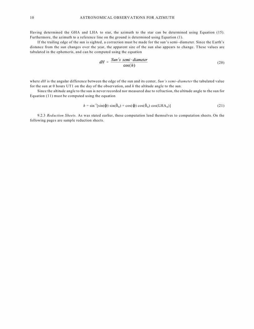
(20)

Having determined the GHA and LHA to star, the azimuth to the star can be determined using Equation (15).

Furthermore, the azimuth to a reference line on the ground is determined using Equation (1).

If the trailing edge of the sun is sighted, a correction must be made for the sun’s semi–diameter. Since the Earth’s

distance from the sun changes over the year, the apparent size of the sun also appears to change. T hese values are

tabulated in the ephemeris, and can be computed using the equation

where dH is the angular difference between the edge of the sun and its center, Sun’s semi–diameter the tabulated value

for the sun at 0 hours UT1 on the day of the observation, and h the altitude angle to the sun.

Since the altitude angle to the sun is never recorded nor measured due to refraction, the altitude angle to the sun for

Equation (11) must be computed using the equation

h = sin -1[sin(N) sin(*') + cos(N) cos(*') cos(LHA')] (21)

9.2.3 Reduction Sheets. As was stated earlier, these computation lend themselves to computation sheets. On the

following pages are sample reduction sheets.

REDUCTION SHEET FOR POLARIS OBSERVATIONS 11

DATE: _____/ _____/ _________

LATITUDE:_____/ _______’ _________” LONG ITUDE:_____/ _______’ _________”

STOPWA TCH START TIM E= _______: _______UTC DUT correction: ____s

STOPWA TCH STOP TIM E= _______: _______UTC ERRO R: ____s

UT = STOPWATCH STA RT TIM E + DUT correction = _____: ______ : ______

)T = STOPWATC H STOP TIME ! STO PW ATCH START TIM E = ____: _____

OBSERVATIONS

Pointing E.T. UT1 Horizontal angle

1

2

3

4

5

6

where E.T. is the stopwatch elapsed time from the beginning of the observation session,

UT1 = UT + ET + ERROR×UT/)T

GHA0 = _______/ ______’ _________” GHA24 = _______/ ______’ _________”

*0 = _______/ ______’ _________” *24 = _______/ ______’ _________”

POINTING GHA LHA * Azimuth p Azimuth Line

1

2

3

4

5

6

Mean of line’s azimuth =


9.3 SAMPLE COMPUTATIONS

Table 4 contains a set of field notes that were taken on the sun. The latitude and longitude of the observation station were

41°18'27" N and 76°01 '03" W. What are the individual azimuths of the lines, their mean and standard deviation?

Table 4 Sample set of field notes for Solar observation.

Observation of Sun

Instrument @ 21002 Sighted 21003

Watch start: 15:43 Date: 12/07/92

Watch stop: 16:00 DUT corrn +0.3 seconds

Pointing Position Elapsed time H. Circle

21003 D 0/ 00' 00"

' D 0:04:15.9 20/ 24' 24"

' D 0:05:04.1 20/ 36' 21"

' D 0:07:01.3 21/ 05' 00"

' R 0:14:36.6 202/ 57' 36"

' R 0:15:16.5 203/ 07' 21"

' R 0:16:03.1 203/ 19' 02"

21003 R 180/ 00' 00"

Solution:

DATE: 12/ 07 / 1992

LATITUDE: 41° 18’ 27” LONGITUDE: 76° 01’ 03”

STOPW ATCH START TIM E= 15: 43 UTC DUT correction: +0.3 s

STOPW ATCH STOP TIM E= 16: 01 UTC ERR OR: 0s

UT = STOPWATCH STA RT TIM E + DUT correction = 15 : 43 : 00.3

)T = STOPWATCH STO P TIM E - STOPWATCH START TIM E = 0: 18

OBSERVATIONS

Pointing E.T. UT1 Horizontal angle

1 0:04:15.9 15:47:16.2 20° 24' 24"

2 0:05:04.1 15:48:04.4 20° 36' 21"

3 0:07:01.3 15:50:01.6 21° 05' 00"

4 0:14:36.6 15:57:36.9 22° 57' 36"

5 0:15:16.5 15:58:16.8 23° 07' 21"

6 0:16:03.1 15:59:03.4 23° 19' 02"

where E.T. is the stopwatch elapsed time from the beginning of the observation session,

UT1 = UT + ET + ERROR×UT/)T


GHA0 = 182° 08N 52.3O GHA24 = 182° 02N 22.5O*0 = !22° 36N 40.2O *24 = !22° 43N 10.9O

POINTING GHA LHA * Azimuth p Azimuth Line

1 58°53'38.9" 342°52'35.9" !22°41'00.04" 162°41'29" 141°59'17"

2 59°05'41.7" 343°04'38.7" !22°41'00.26" 162°53'18" 141°59'08"

3 59°34'59.1" 343°33'56.1" !22°41'00.78" 163°22"05" 141°59'15"

4 61°28'46.6" 345°27'43.6" !22°41'02.81" 165°14'34" 141°59'04"

5 61°38'44.9" 345°37'41.9" !22°41'02.99" 165°24'28" 141°59'04"

6 61°50'23.7" 345°49'20.7" !22°41'03.20" 165°36'02" 141°59'07"

Mean of line’s azimuth = 141°59'10.7"

9.3.1 Computations Using Software. With the advent of the personal computer and the programmable calculator

have come a multitude of programs capable of reducing celestial observations for azimuth. The advantage of the

hand–held calculator lies in its ability to reduce the observations d irectly in the field. In fact, data collectors based on

the programmable hand–held calculator can provide the user with an internal clock and maintain a running average of

the azimuth of the line while the observations are being made. This capability offers the user the advantage of recognizing

a poor pointing immediately in the field .

Computer programs have also been written to reduce observations for azimuth. Below is a sample listing from

WolfPack.

--------------------------- Reduction of Solar Shots---------------------------

Observer's Astronomic Position:

Latitude = 41°18'27.0"

Longitude = 76°01'3.0"

Semi-diameter at 0h UT : 0°16'15.7" sighting trailing edge.

Stop Watch Start Time, UTC: 15:43:00 .0

DUT correction: 0.3sec

GHA of Sun at 0h UT : 182°08'52.30"

GHA of Sun at 24h UT : 182°02'22.50"

Declination of Sun at 0h UT : -22° 36'40.20"

Declination of Sun at 24h UT : -22° 43'10.90"

Pointing Time Hor. Angle* Declination L H A Azimuth to Star Az of Line

-----------------------------------------------------------------------------------------------------------

1 15:47:16.2 20°42'13" -22° 41'0.04" 342°52'35.9" 162°41'29" 141°59'17"

2 15:48:04.4 20°54'10" -22° 41'0.26" 343°04'38.7" 162°53'18" 141°59'08"

3 15:50:01.6 21°22'50" -22° 41'0.78" 343°33'56.1" 163°22'05" 141°59'15"

4 15:57:36.9 23°15'29" -22° 41'2.81" 345°27'43.6" 165°14'34" 141°59'04"

5 15:58:16.8 23°25'14" -22° 41'2.99" 345°37'41.9" 165°24'28" 141°59'13"

6 15:59:03.4 23°36'56" -22° 41'3.20" 345°49'20.7" 165°36'02" 141°59'07"

----------------------------------------------------------------------------------------------------------

Average Astronomic Azimuth of Line » 141°59'10.7"

Deviation from the mean » ±4.58"


Figure 15 Error due to

instrument leveling error.

Figure 16 Altitude angle versus angular

error.

Figure 17 Precise leveling

* - For sun shots with leading/trailing edges,

horizontal angles corrected for sun's semi-diameter.

10 ERRORS IN CELESTIAL OBSERVATIONS

For an experienced observer doing celestial observations, the largest source of errors

comes from misleveling the instrument. This error is small for typical boundary surveys,

but becomes quite large in astronomical observations due to the presence of large vertical

angles. Figure 14 shows the conditions present at the time of observation for an instrument

that is misleveled. Notice that for an instrument having a bubble with sensitivity of : which

is misleveled by fd fractional parts of a division, the error in the horizontal angle due the

scope not p lunging vertically is

(22)

where h is the altitude angle, and , the error in the horizontal circle reading.

A plot showing the size of the error (e) versus the size of the altitude angle (h) is

depicted in Figure 15. Note how fast the error size increases with increasing angle. Since Polaris has an altitude angle

approximately equal to the latitude of the observer, and since the sun can

reach altitudes nearing 90° for parts of the continental U.S. during the summer

months, the leveling of the instrument becomes a crucial factor in the

accuracy of the derived azimuth.

A method used to precisely level an instrument involves using the

instrument’s vertical compensator and is as follows

(a) As shown in Figure 16, set the leveling screws of the instrument in

relation the position of the celestial object so that it is perpendicular

the scope of the instrument

(b) Precisely level the instrument using normal leveling procedures and

the horizontal plate bubble

(c) W ith the vertical circle clamped, read and record the zenith angle

(d) Rotate the instrument 180° from its initial position

(e) Read the zenith angle again.

(f) Average the two zenith angles

(g) Using the single leveling screw (a), adjust the level of the instrument so that the

average zenith angle is obtained on the vertical circle.

Astronomy

Documents

Transcript of Astronomy