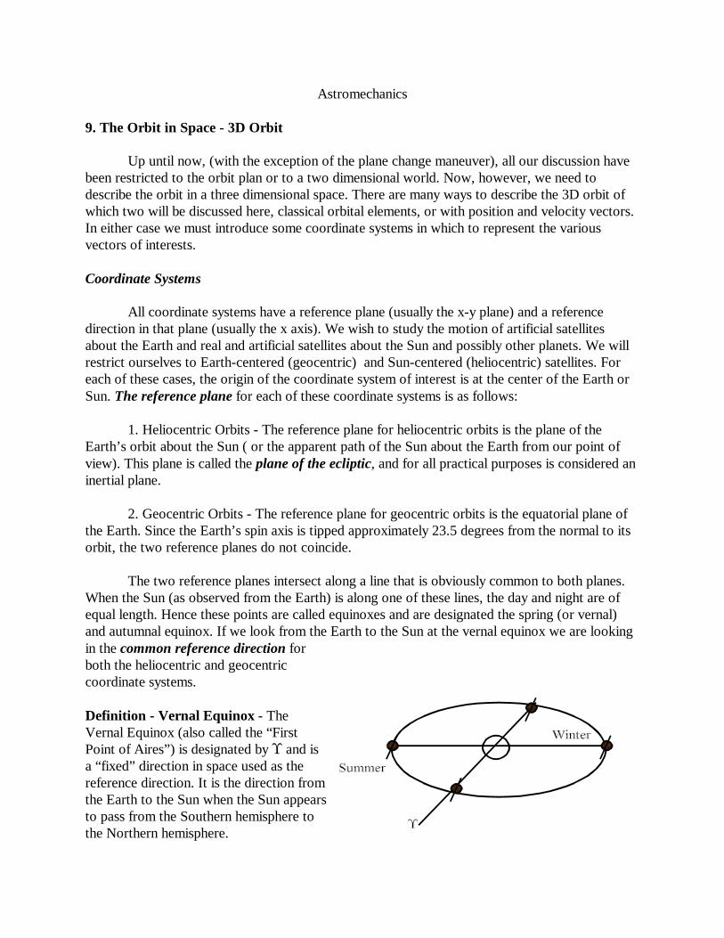
Astromechanics

9. The Orbit in Space - 3D Orbit

Up until now, (with the exception of the plane change maneuver), all our discussion havebeen restricted to the orbit plan or to a two dimensional world. Now, however, we need todescribe the orbit in a three dimensional space. There are many ways to describe the 3D orbit ofwhich two will be discussed here, classical orbital elements, or with position and velocity vectors.In either case we must introduce some coordinate systems in which to represent the variousvectors of interests.

Coordinate Systems

All coordinate systems have a reference plane (usually the x-y plane) and a referencedirection in that plane (usually the x axis). We wish to study the motion of artificial satellitesabout the Earth and real and artificial satellites about the Sun and possibly other planets. We willrestrict ourselves to Earth-centered (geocentric) and Sun-centered (heliocentric) satellites. Foreach of these cases, the origin of the coordinate system of interest is at the center of the Earth orSun. The reference plane for each of these coordinate systems is as follows:

1. Heliocentric Orbits - The reference plane for heliocentric orbits is the plane of theEarth’s orbit about the Sun ( or the apparent path of the Sun about the Earth from our point ofview). This plane is called the plane of the ecliptic, and for all practical purposes is considered aninertial plane.

2. Geocentric Orbits - The reference plane for geocentric orbits is the equatorial plane ofthe Earth. Since the Earth’s spin axis is tipped approximately 23.5 degrees from the normal to itsorbit, the two reference planes do not coincide.

The two reference planes intersect along a line that is obviously common to both planes.When the Sun (as observed from the Earth) is along one of these lines, the day and night are ofequal length. Hence these points are called equinoxes and are designated the spring (or vernal)and autumnal equinox. If we look from the Earth to the Sun at the vernal equinox we are lookingin the common reference direction forboth the heliocentric and geocentriccoordinate systems.

Definition - Vernal Equinox - TheVernal Equinox (also called the “FirstPoint of Aires”) is designated by K and isa “fixed” direction in space used as thereference direction. It is the direction fromthe Earth to the Sun when the Sun appearsto pass from the Southern hemisphere tothe Northern hemisphere.

Definition - Celestial Sphere - Thecelestial sphere is an imaginary sphere ofinfinite radius that is centered at the originof the coordinate system of interest. Theposition of the satellites and stars areprojected onto the celestial sphere and canbe located by specifying two angles: onemeasured in the reference plane from thereference direction, and the other in a planeperpendicular to the reference plane. Thetwo angles are designated as:

This coordinate system is often used byastronomers to locate stars in the heavens.

Orbital Elements

Recall that we started our two-body problem with a vector, second order, ordinarydifferential equation that requires six constants of integration to obtain a complete solution to theproblem. We extracted these six constants in our previous work. By combining these constants incertain ways, we can arrive at a different set of six independent constants. There are many ways todo these combinations and permutations and hence there are a large number of different groups ofsix constants. Whatever the final selection is, these six constants are called the orbital elements.Here we will look at the “classical” set of orbital elements.

The classic orbital elements includetwo elements to locate the plane of theorbit in space, two to describe the size andshape of the orbit, one to orient the orbitin the plane, and the last to locate thesatellite in the orbit. The elements are:

a Semi-major axise Orbit eccentricityi the orbit inclinationS the right ascension of the

ascending node(Or longitude of the ascendingnode)

T argument of periapsisJ time of periapsis passage

The orbit plane and the reference plane (equatorial plane) intersect in a line called the “lineof nodes”. The end of this line where the satellite moves from the southern hemisphere to thenorthern hemisphere is called the ascending node. It takes two angles to orient the orbit plane inspace, the angle between the vernal equinox and the ascending node, S, called the longitude ofthe ascending node (or right ascension of the ascending node), and the angle between the normalto the orbit plane (along the angular momentum vector), and the normal to the reference plane,the z or north-pointing axis, called the inclination angle, i. As will be shown later, these twoangles are directly related to the angular momentum vector as might be expected. We should alsonote that we define direct and retrograde orbits in the following manner:

Direct orbitRetrograde orbitPolar orbit

The energy of the orbit gives us the size of the orbit, or the semi-major axis, a, and themagnitude of the angular momentum (combined with the energy) give us the shape or eccentricityof the orbit. Finally the orbit is oriented in the plane by defining the angle, T, between the line ofthe ascending node, and the line passing through the periapsis of the orbit. This angle is called theargument of periapsis and is measured in the plane of the orbit.

The final constant is the time of periapsis passage, J, that allows us to determine where thesatellite is in orbit at some given time, t.

These six elements are called the “classic” orbital elements and fully describe the orbit andthe position of the satellite in orbit. Hence if we know the elements and time, a, e, i, S, T, J, andt, we can locate the orbit and the satellite in space. These elements are convenient to use becausethey bring the physical picture to mind and allow one to visualize the orbit and its orientation.However, often other “elements” are used to describe orbits. Rather than use t and J, it isconvenient to us the mean anomaly M or more properly, the mean anomaly at some specified timeor epoch, M0. Hence the orbital elements are a, e, i, S, T, and M0. (Note that M0 may beconsidered an element since it is a constant). In either case, in order to determine the satellite’sposition, we are required to solve Kepler’s equation in order to determine E, and subsequently, <,the true anomaly. It is convenient to designate the true anomaly, or more properly, the trueanomaly at some specified time or epoch as an “element.” We can completely describe the orbitand satellite position is space if we know the “elements” a, e, i, S, T, and <0. In this form, we donot have to solve Kepler’s equation and thus this form will be used extensively here forconvenience. However, you should be aware that the true anomaly, <, is not an orbital elementwhile <0 may be considered an element. Use of the true anomaly as an orbital element avoids thenecessity of solving the Kepler equation. If the classic orbital elements and time are given, < and<0 would be calculated from the Kepler and related equations given a, e, J, and t.

Alternate Orbital Elements

A cursory glance at the classical orbital elements will reveal that under certaincircumstances, such as an equatorial orbit or a circular orbit (or both), that some elements are

undefined. Motivated by this occurrence, alternative elements have been defined. Again, these arecombinations of existing elements.

u0 = T + <0 argument of latitude at epoch

This also defines the time varying version of this element

u(t) = T + <(t) argument of latitude

We also have

j = S + T longitude of periapsis

R0 = j + <0 true longitude at epochR(t) = j + <(t) true longitude

<0 true anomaly at epoch<(t) true anomaly

The Three Dimensional Problems

There are two problems of interest that we can study in this three dimensionalenvironment

1) Given: the orbital elements a, e, i, S, T, J, and the time t (or another set ofelements),

Find: the position and velocity vectors, .

2) Given: the position and velocity vectors, ,Find: the orbital elements a, e, i, S, T, J.

Problem (2) is called the orbit determination problem.

Problem (1) Given the orbital elements - find the position and velocity vectors

The problem requires that we find the position and velocity vectors in an inertialcoordinate system. The approach is to find the representation of the position and velocity vectorsin some convenient coordinate system and then find a transformation that allows us to find theirrepresentation in the desired “inertial” system. This idea of transferring the representation ofvectors from one system to another is an extremely useful concept and is used in many otherastromechanics problems as well as in many other disciplines.. We relate these tworepresentations in the two different coordinate systems to each other by use of what are calledtransformation matrices.

Transformation Matrices

In order to develop the concept of a transformation matrix we will look at the

representation of a generic vector, , in two different coordinate systems labeled (1) and (2). In addition, coordinate system (2) is rotated about the z axis an amount 0 with respect to system(1). The vector representation in each coordinate system is given by:

and

where the superscript indicates thecoordinate system in which the quantity isrepresented. We can relate thecomponents of the vector represented insystem (2) to the components of the samevector written in system (1) by observingthe figure and recalling that thecomponent of any vector along a givenline is found by dropping a perpendicular to that line from the tip of the vector. In any case wehave:

(1)

These equations can be more presented more compactly using a matrix formulation:

(2)

or

(3)

where is the transformation matrix from system (1) to system (2). Since in this case axes

system (2) is rotated an amount 0 from system (1), is called the transformation matrix for a z

rotation or the z rotation transformation matrix.

In a similar manner we can develop a transformation matrix for a single rotation about thex, y, and z axes. The results of such activity are given by:

(4)

The matrices presented in Eq. (4) are the fundamental rotation matrices and represent thetransformation matrices that allow us to transform the representation of a given vector in system(1) to the representation of the same vector in system (2) for a particular single rotation about thespecified axis.

The orientation of one axes system with respect to another axes system can always bedefined as a sequence of rotations about these individual axes. In general it takes three successiverotations to go from one system to an arbitrary orientation of the new system. However in somecases it may take less or for convenience, more than three. The sequence of rotations is important,and must be specified. Generally we label the x axis as the “1" axis, the y axis as the “2" axis andthe z axis as the “3" axis. The sequence of rotation is then designated as the 321 or 313 sequence.There are 12 possible 3 rotation sequences. Of interest to us is the transformation from someconvenient axes system in which it is easy to represent the position and velocity to the standardinertial system where the vernal equinox serves as the “x” axis and the north point axis as the “z”axis.

The Local Coordinate System

For convenience we will define the “local” coordinate system in the following way: The

origin of the system is geocentric (heliocentric or planetocentric) with the x axis point out theradius vector. The y axis is at right angles to the x axis and lies in the plane of the orbit. The z axisis normal to the plane of the orbit and is aligned with the angular momentum vector. The threeaxes form a right handed set. Therepresentation of the position vector insuch an axis system is extremely simple:

(5)

and the velocity is simply:

(6)

We now seek the sequence of rotationsthat it would take to align the “local” axessystem with the standard inertial system.From the two figures we can establish thatthe following sequence of rotations willalign the local axes system with theclassical inertial system:

1) rotate [ ] about the zR

axis to x’y’z’ set (x axis nowaligned with line of nodes)

2) rotate (- i) about the x’ axis to thex”y”z” set (x axis aligned with lineof nodes, and the z axis pointingnorth)

3) rotate (- S) about the z” axis to the inertial m YZ axes.

The transformation matrix to take the simple representations of the position and velocity vectorsgiven by Eqs. (5) and (6) into a representation of the same vectors in the inertial system areobtained by carrying out the transformations one rotation at a time. We also note the following(well known) identities:

(7)

The transformation matrix has the form:

(8)

with a similar form for the velocity.

We can write out Eq. (8) in more detail, and can multiply the matrices together to get the finaltransformation matrix.

(9)

where is the transformation matrix given by:

(10)

Equation (10) provides the complete transformation matrix for transferring vectorsrepresented in the local system to the same vectors represented in the inertial system. In order toget our desired results, we must multiply the matrix by the position and velocity vectors. For theposition vector the result is just r times the first column of the transformation matrix:

(11)

The velocity vector in classical inertial coordinates is

(12)

where from previous work we have:

(15)

(16)

(13)

Hence given the orbital elements and time, a, e, i, S, T, J, and t, we can use Kepler’sequation to solve for the true anomaly, <, and use Eqs. (11) and (12) to obtain the position and

velocity vectors represented in the classical inertial system.

Perifocal Coordinate System

At this point we can introduce the perifocal coordinate system. In the two-body problemthis is also an inertial coordinate system. Its origin is at the focus (geocentric or heliocentric) ofthe orbit with the x axis pointing in the direction of the periapsis, the y axis in the orbit plane, andthe z axis aligned with the angular momentum vector, the three axes forming a right-hand set. Itshould be clear from the figure above that the transformation from the local coordinate system tothe perifocal coordinate system is obtained by a simple rotation of about the z axis. Thereforethe transformation matrix from local to perifocal axes is given by:

(14)

Then the position and velocity vectors in the perifocal system can be determined to be:

For the position vector we have:

and for velocity we have:

Equations (15) and (16) give the position and velocity in the peri-focal coordinate system in termsof the true anomaly, .

It is useful to have these same components of position and velocity in terms of theeccentric anomaly. In order to do this we need to go back to the basic definitions and geometrythat we developed for introducing the eccentric anomaly. Eventually we will need an expressionfor the time derivative of the eccentric anomaly. We will develop that next. First recall that themagnitude of the position vector is given by

(17)

From Kepler’s equation we have:

(18)

Taking the derivative with respect to time we get:

(19)

Then we can determine .

(20)

In the local system we have:

where (21)

To determine the components of the position and velocity vectors in the perifocal systemwe can go directly to the components already determined in the eccentric anomaly development.The position vector is given (from the geometry and definitions) and the velocity vector isobtained by taking the derivative of the components and using the expression developedpreviously for the time derivative of E.

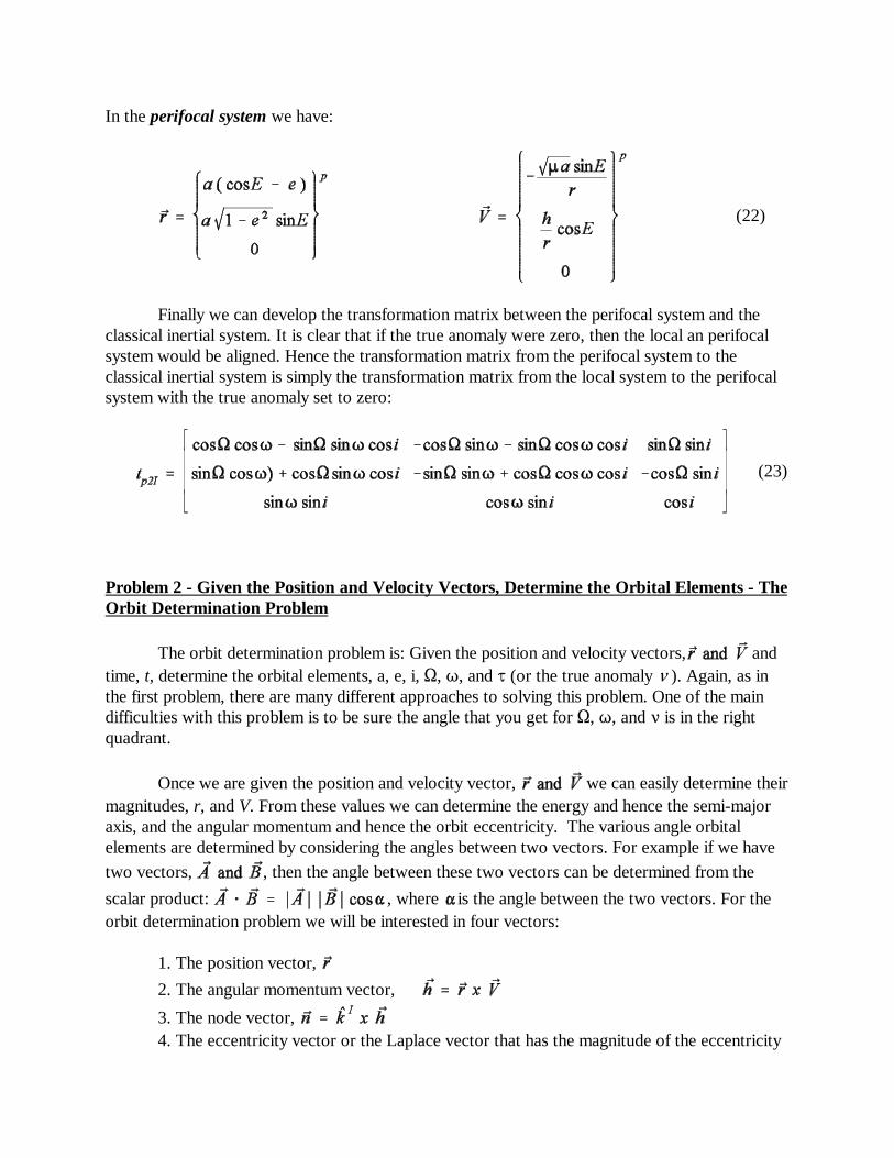
In the perifocal system we have:

(22)

Finally we can develop the transformation matrix between the perifocal system and theclassical inertial system. It is clear that if the true anomaly were zero, then the local an perifocalsystem would be aligned. Hence the transformation matrix from the perifocal system to theclassical inertial system is simply the transformation matrix from the local system to the perifocalsystem with the true anomaly set to zero:

(23)

Problem 2 - Given the Position and Velocity Vectors, Determine the Orbital Elements - TheOrbit Determination Problem

The orbit determination problem is: Given the position and velocity vectors, andtime, t, determine the orbital elements, a, e, i, S, T, and J (or the true anomaly < ). Again, as inthe first problem, there are many different approaches to solving this problem. One of the maindifficulties with this problem is to be sure the angle that you get for S, T, and < is in the rightquadrant.

Once we are given the position and velocity vector, we can easily determine theirmagnitudes, r, and V. From these values we can determine the energy and hence the semi-majoraxis, and the angular momentum and hence the orbit eccentricity. The various angle orbitalelements are determined by considering the angles between two vectors. For example if we have

two vectors, , then the angle between these two vectors can be determined from the

scalar product: , where is the angle between the two vectors. For theorbit determination problem we will be interested in four vectors:

1. The position vector,

2. The angular momentum vector,

3. The node vector, 4. The eccentricity vector or the Laplace vector that has the magnitude of the eccentricity

and is directed in the direction of the periapsis,

We need to develop the expression for this eccentricity vector. This development issomewhat abstract in that there is little motivation to carry out the steps as indicated. One shouldremember that orbital mechanics has been around since the days of Newton so there has been a lotof “playing” with the equations. When such activity lead to a result, the usual description of thedevelopment is “elegant.” What follows is an elegant derivation of the eccentricity vector.One of the tools we will use is the vector triple product identity or the bac - cab identity:

(24)

We will start with the basic equation of motion:

(25)

We can now take the cross product with the angular momentum vector:

(26)

where we have made use of the fact that for any vector, . The left and right hand

sides of Eq. (26) are perfect differentials, so we have:

(27)

Or integrating:

(28)

We now take the scalar product of Eq. (28) with to get:

(29)

If we keep the order of the terms the same, we can interchange the dot and cross in the first termand we get:

(30)

We can solve Eq. (30) for the radius, r

(31)

From Eqs. (29-31) we see that the angle between is , the true anomaly, and that the

magnitude of the vector , . Consequently, is a vector that has a magnitude equal tothe eccentricity and point in the direction of the periapsis. Hence we can define the eccentricity

vector from . Then from Eq. (28) we have:

(32)

or

The Eccentricity Vector

(33)

Orbit Determination Algorithm ( Given , , and t )

We will assume that we are given or can determine the position and velocity vectors interms of the classic inertial coordinates:

Given: and

1. Determine the magnitudes of the position and velocity vectors:

2. Determine the energy equation and the semi-major axis:

(34)

However, since there is a remote possibility of a parabolic orbit (or a near parabolic orbit) oneusually calculates the quantity (from the energy equation):

(35)

Then, if , either quantity will equal zero and the algorithm will continue.

3. Compute the angular momentum vector and its magnitude:

(36)

4. Compute the eccentricity vector and its magnitude::

(37)

The last two equations can be used as a check on progress.

5. Compute the inclination:

(38)

The inclination always lies between 0 and 180 deg. For i > 90 deg the orbit is retrograde

6. Compute the nodal vector and its magnitude:

(39)

7. Compute the longitude of the ascending node ( right ascension of the ascending node)

(40)

Here, can be positive or negative. If positive, must lie in the first or fourth quadrant, andif negative, in the second or third. This fact, plus the information gained from the sign of should

be enough to determine which is the correct quadrant for .

8. Compute the argument of periapsis:

(41)

The quadrant for can be determined in a similar manner as for the longitude of the ascendingnode, check to see in which half exists, then the sign of to determine the quadrant.

9. Determine the true anomaly:

(42)

Again, the quadrant of the true anomaly can be determined by checking and determining thehalf, then checking the sign of to obtain the quadrant.

10. Determine the time of periapsis passage:

Often times we can stop at step 9 since we know just about everything we need to aboutthe orbit. However, if we want to determine the sixth element, the time of periapsis passage weneed to use the current time, and Kepler’s equation. We can determine the eccentric anomaly

from:

(43)

Again one must be careful to get the right quadrant. The rule here is that the true and eccentricanomalies are always in the same half of the orbit. Once we determine the eccentric anomaly, wecan solve for the time of periapsis passage from Kepler’s equation:

(44)

If the orbit is circular ( and is not defined ) or if we just want to determine theargument of latitude, we can determine it, in general, as follows:

(45)

or if , .

Special Cases

As indicated previously, if the eccentricity and/or the inclination is zero, then some of theclassic orbital elements to do not exist. If this is the case, then it will show up in our algorithm byfinding zeros in the denominator of some of the terms. We an summarize some of thesestatements in a table:

Quantity Doesn’t Exist If:

n = 0

n = 0e = 0

e = 0

Case :Longitude of periapsis:

(46)

otherwise if

Case Argument of latitude:

(47)

otherwise if

Case True longitude:

(48)

Otherwise if

Example:

Given: ;

1. Determine magnitudes:

;

2. Calculate Energy and Semi-major axis:

3. Calculate angular momentum and its magnitude:

4. Compute the eccentricity vector and its magnitude:

or

5. Compute the inclination:

(Retrograde)

6. Compute the nodal vector:

Since n = 0, then the longitude of the ascending node and argument of periapsis are undefined:

7. Calculate longitude of the ascending node:

8. Calculate argument of periapsis:

Since n = 0 we can calculate the longitude of the periapsis

However, so j > 180 deg. Since the cosine of j > 0, the angle must be in the

fourth quadrant: j = 306.87 degrees

9. Calculate the true anomaly:

Since , must be in first half, hence: