AST 6416: Physical CosmologyInstructor: Gonzalez

Fall 2009

This document contains the lecture notes for the graduate level cosmology course at theUniversity of Florida, AST 6416. The course is 15 weeks long, with three class periodsper week (one on Tuesday and two on Friday). These notes are based upon a collection ofsources. The most notable of these are lecture notes from George Blumenthal and HenryKandrup, and the textbooks by Coles & Lucchin (2002), Peacock (1999), and Peebles (1993).

1 Introduction, Early Cosmology

Week 1 Reading Assignment: Chapter 1

1.1 Course Overview

Cosmology, defined as man’s attempt to understand the origin of the universe, is as old asmankind. Cosmology, as a field of scientific inquiry, is one of the newest of topics. The firsttheoretical underpinnings of the field date to the dawn of the 20th century; a significantfraction of the landmark cosmological observations have occurred in the past two decades— and the field certainly holds a plethora of fundamental unanswered questions. It is onlyduring this past century that we have gained the ability to start answering questions aboutthe origin of the universe, and I hope to share with you some of the excitement of this field.

The title of this course is Physical Cosmology, and the central aim of this semester will befor you to understand the underlying physics that defines the formation and evolution of theuniverse. We will together explore the development of Big Bang cosmology, investigate thesuccesses (and failures) of the current paradigm, and discuss topics of current relevance. Bythe end of the course, you will have a basic understanding of the foundations upon which ourcurrent picture of the universe is based and (hopefully) a sense of the direction in which thisfield is headed. What you will not have is comprehensive knowledge of the entire disciplineof cosmology. The field has grown dramatically in recent years, and a semester is sufficienttime to cover only a fraction of the material. This semester will be primarily taught from atheoretical perspective, with limited discussion of the details of the observations that havehelped define our current picture of the universe.

General Relativity is the foundation that underpins all of modern cosmology, as it definesthe structure of spacetime and thereby provides the physical framework for describing theUniverse. I realize that not all of you have taken a course in GR; and a detailed discussionof GR is beyond the scope of this class. Consequently, I will tread lightly in this area, andGR will not be considered a prerequisite for this class. For many of the key results, wewill use pseudo-Newtonian derivations to facilitate intuition (which is useful even if you doknow GR). In practice, this detracts very little from the scope of the course. Once we have

1

established a few fundamental equations, the bulk of the semester will be quite independentof one’s knowledge of General Relativity. For those of you who wish to learn more aboutGeneral Relativity, I refer you to PHZ 6607.

Finally, please review your copy of the syllabus for the semester. You will see that thetextbook is Coles & Lucchin. The advantages of this text are that it is generally readable andshould serve as a good reference source for you both for this class and in the future. Moreover,this text is used both for my course and for Observational Cosmology. Be aware howeverthat the organization of this course does not directly parallel the organization of the book– we will be jumping around, and sometimes covering material in a different fashion thanthe text. The first half of the semester will be dedicated to what I would call “classical”cosmology, which broadly refers to the fundamental description of the universe that wasdeveloped from 1916-1970 – the global structure of the universe, expansion of the universe,and development of the Big Bang model, Big Bang nucleosynthesis, etc. The second half ofthe semester will focus upon more recent topics in the field – things such as dark matter,dark energy, inflation, modern cosmological tests, and gravitational lensing. I emphasizethat the division between the two halves of the semesters is only a preliminary plan, andschedule may shift depending on the pace of the course. Homework will be assigned everytwo weeks, starting on Friday, and will comprise 50% of your grade. I strongly encourage youto work together on these assignments. Astronomy and cosmology are collaborative fieldsand you are best served by helping each other to learn the material. Make sure though thatyou clearly understand everything you write down – otherwise you will be poorly served forthe exam and the future. The final will be comprehensive for the semester and account forthe other 50%.

1.2 The Big Questions

Before we begin, it is worth taking a few moments to consider the scope of the field ofcosmology by considering, in broad terms, the aim of the subject. More so than most otherfields, cosmology is all encompassing and aims for a detailed understanding of the universeand our place therein. Fundamental questions that the field aims include:

• What is the history of the Universe? How did it begin? How did the structuresthat we see today – matter, galaxies, and everything else – come to be?

• What is the future of the Universe? What happens next? How does the Universeend, or does it end?a

• How does the Universe, and the matter/energy it contains, change withtime?

• What are the matter/energy constituents of the Universe and how werethey made?

• What is the geometry of the Universe?

2

• Why are the physical laws in the Universe as they are?

• What, if anything, exists outside our own Universe?

Clearly an ambitious set of questions. We by no means have complete answers to all ofthe above, but it is remarkable the progress – and rate of progress – towards answers that hastranspired in recent times. In this course we will touch upon all these topics, but primarilyfocus upon the first five.

1.3 Olbers’ Paradox

And so with that introduction, let us begin. Let us for a moment step back 200 years to1807. Newtonian physics and calculus were well-established, but electromagnetism was stillover 50 years in the future, and it would be a similar year before Monsieur Messier wouldbegin to map his nebulae (and hence the concepts of Galaxy and Universe were essentiallyequivalent). Copernicus had successfully displaced us from the center of the solar system,but our position in the larger Universe was essentially unknown. At the time, as wouldremain the case for another 100 years, cosmology was the realm of the philosopher – buteven in this realm one can ask physically meaningful questions to attempt to understandthe Universe. Consider Olbers’ Paradox, which was actually first posited in ancient Greecebefore being rediscovered by several people in the 18th and 19th century. When Olbersposed the paradox in 1826, the general belief was the Universe was infinite, uniform, andunchanging (“as fixed as the stars in the firmament”). The question that Olbers asked was:Why is the night sky dark?

Let us make the following assumptions:

1. Stars (or in a more modern version galaxies) are uniformly distributed throughout theuniverse with mean density n and luminosity L. This a corollary of the CosmologicalPrinciple, which we will discuss in a moment.

2. The universe is infinitely old and static, so n = L = 0.

3. The geometry of space is Euclidean. And in 1800, what else would one even consider?

4. There is no large scale systematic motion of stars (galaxies) in the Universe. Specifi-cally, the Universe is not expanding or contracting.

5. The known laws of physics, derived locally, are valid throughout the Universe.

For a Euclidean geometry, the flux from an object is defined simply as

f =L

4πr2, (1)

where L is the luminosity and r is the distance to the object. In this case, the total incidentflux arriving at the Earth is

3

ftot =∫ ∞

04πr2dr

(

nL

4πr2

)

=∞ (2)

The incident flux that we observe should therefore be infinite, as should the energydensity, < u >≡ f/c. Clearly the night sky is not that bright!

Can we get around this by including some sort of absorption of the radiation? Addingan absorbing dust between us doesn’t help much. For a static, infinitely old universe (as-sumption 2), the dust must eventually come into thermodynamic equilibrium with the starsand itself radiate. This would predict a night sky as bright as the surface of a typical star.

We get the same result if we include absorption by the stars themselves (through theirgeometric cross section). Specifically, consider the paradox in terms of surface brightness.For a Euclidean geometry, surface brightness (flux per unit solid angle) is independent ofdistance since

I ≡ f/dΩ =(

L

4πr2

)

/

(

πd2

r2

)

=L

4π2d2, (3)

where d is the physical size of the object. If the surface brightness is constant, and there is astar in every direction that we look (which is a the logical result of the above assumptions),then every point in space should have the same surface brightness as the surface of a star –and hence Tsky ≈ 5000 K. That the sky looks dark to us tells us that Tsky < 1000 K, andfrom modern observations of the background radiation we know that Tsky = 2.726 K.

Which assumption is wrong?! Assumption 1 is required by a Copernican view of the Uni-verse. We now know that the stars themselves are not uniformly distributed, but the galaxydensity is essentially constant on large scales. We are also loathe to abandon assumption 5,without which we cannot hope to proceed. Assumption 3, Euclidean geometry, turns out tobe unnecessary. For a non-Euclidean space, the surface area and volume elements within asolid angle dΩ are defined as:

dA = r2f(r,Ω)dΩ (4)

anddV = d3r = r2f(r,Ω)drdΩ. (5)

Therefore, from a given solid angle dΩ,

< u >Ω=∫

r2drf(r,Ω)(

n

c

)

(

L

r2f(r,Ω)

)

=∫

drnL

c, (6)

independent of f(r,Ω).Relaxing assumption 2 (infinite and static) does avoid the paradox. If the Universe is

young, then:

• Absorption can work because the dust may not be hot yet.

• Stars may not have shined long enough for the light to reach us from all directions.

4

If we define the present time at t0, then we can only see sources out to R = ct0 so

< u >=∫ R

0drnL

c=nLR

c= nLt0, (7)

which is finite and can yield a dark sky for sufficiently small t0.Relaxing assumption 4 can also avoid the paradox. Radial motion gives a Doppler shift

νobserved = νemitted · γ · (1− vr/c). (8)

Since luminosity is energy per unit time, it behaves like frequency squared, i.e.

Lobserved = Lemitted · γ2 · (1− vr/c)2 ≤ Lemitted. (9)

One avoids the paradox if vr ∼ c at large distances. This can be achieved if the Universe isexpanding.

Olbers’ paradox therefore tells us that the universe must be either young orexpanding – or both. In practice, it would be another century before such conclusionswould be drawn, and before there would be additional observational evidence.

2 Definitions and Guiding Principles (Assumptions)

Olber’s paradox has begun to introduce us to some of the fundamental concepts underlyingmodern cosmology. It is now time step forward 100 years to the start of the 20th century,explicitly lay out these concepts, and establish working definitions for terms that we will usethroughout the course.

2.1 Definitions

Let us begin by introducing the concepts of a co-moving observer, homogeneity, andisotropy.

• Co-moving Observer: Imagine a hypothetical set of observers at every point in theuniverse (the cosmological equivalent of test particles). A co-moving observer is definedas an observer who is at rest and unaccelerated with respect to nearby material. Morespecifically, any observer can measure the flow velocity, v(r), of nearby material atany time. If the observer finds v(0) = 0 and v(0) = 0, then the observer is comoving.Co-moving observers are expected to be inertial observers (who feel no force) in ahomogeneous universe. Note, however that all inertial observers are not necessarilycomoving – an inertial observer must have v(0) = 0, but can have v(0) 6= 0.

• Homogeneity: A universe is homogeneous if all co-moving observers would observeidentical properties for the universe. In other words, all spatial positions are equivalent(translational invariance). A simple example of a homogeneous geometry would be the2-D surface of a sphere. Equivalently, an example of an inhomogeneous universe wouldbe the interior of a 3-D sphere, since some points are closer to the surface than others.

5

• Isotropy: A universe is isotropic if, for every co-moving observer, there is no preferreddirection. In other words, the properties of the universe must look the same in all direc-tions. This is equivalent to saying that an isotropic Universe is rotationally invariantat all points. Going back to the same examples from before, the two-dimensional sur-face of a sphere is isotropic – any direction along the surface of the sphere looks thesame. On the other hand, the interior of a 3-D sphere is not isotropic. It is rotationallyinvariant at the center, but for any other point the distance to the surface is shorterfor some directions than others.

So are the conditions of homogeneity and isotropy equivalent? Not quite. One can provethat an isotropic universe is always homogeneous, but the converse is not true. Hereare the proofs.

Assume that the first statement is false, such that there exists a universe that is isotropiceverywhere, but not homogeneous. For an inhomogeneous universe, there must exist someobservable quantity φ(r) that is position dependent. The quantity φ must be a scalar,because if it were a vector it would have a direction and thus violate the assumption ofisotropy. Consider the vector D, defined by

D = ∇φ(r). (10)

Since φ is not a constant, D must be non-zero somewhere. Since D is a vector, it picks outa direction at some point, and therefore the universe cannot appear isotropic to an observerat that point. This contradicts our assumption of an isotropic but inhomogeneous universeand therefore proves that an isotropic universe is always homogeneous.

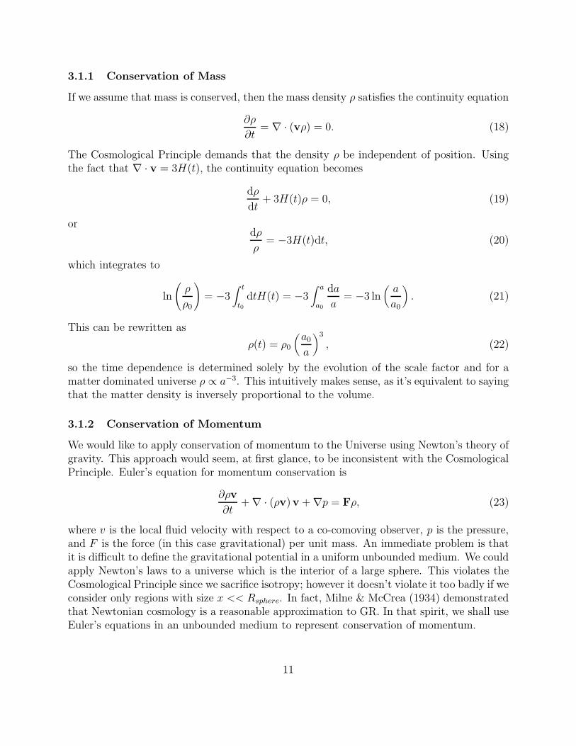
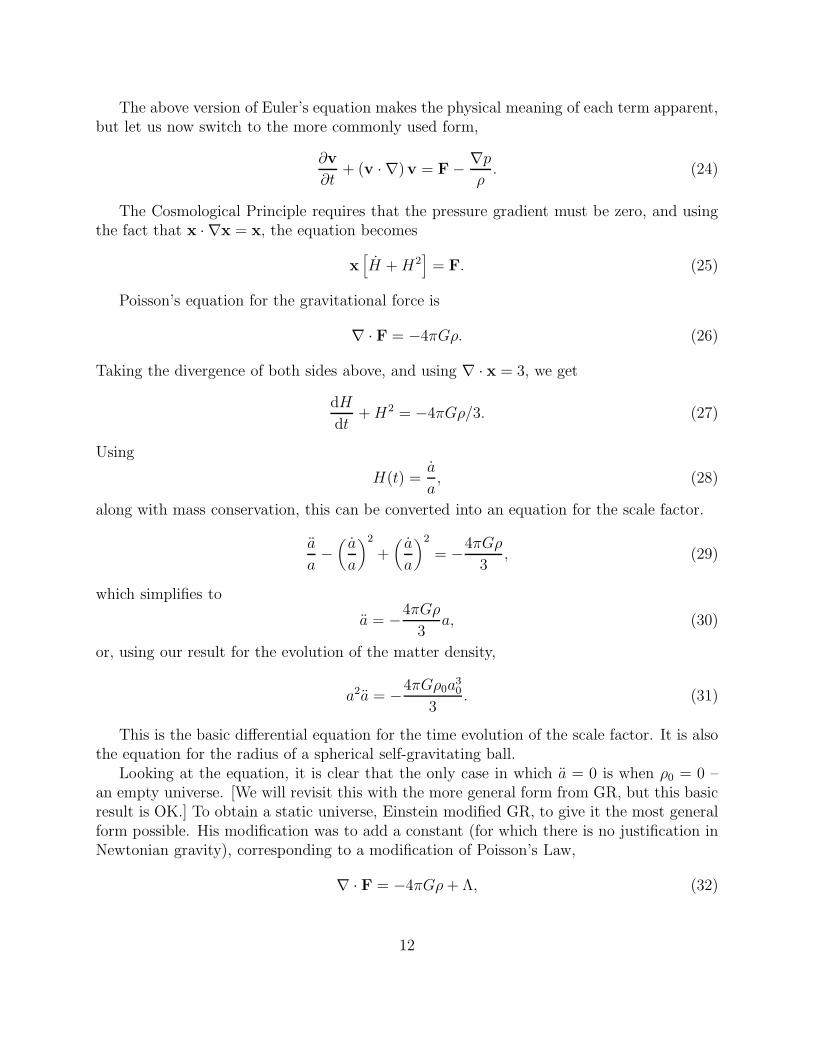
Now, what about the converse statement? How can we have a universe that is homoge-neous but not isotropic. One example would be the 2-D surface of an infinite cylinder (Figure1). The surface is clearly homogeneous (translationally invariant). However, at any pointon the surface the direction parallel to the axis of the cylinder is clearly different from thedirection perpendicular to the axis since a path perpendicular to the axis will return to thestarting point. A few examples of homogeneous, inhomogeneous, isotropic, and anisotropicuniverses are show in Figure 2.

The fact that a geometry is dynamic need not affect its isotropy or homogeneity. Adynamic universe can be both homogeneous and isotropic. Consider the surface of a spherewhose radius is increasing as some function of time. The surface of a static sphere is isotropicand homogeneous. The mere fact that the size of the sphere is increasing in no way picksout a special position or direction along the surface. The same considerations also apply toa uniform, infinite sheet that is being uniformly stretched in all directions.

2.2 The Cosmological Principle

In the early days of cosmology at the start of the 20th century, theoretical developmentwas very much unconstrained by empirical data (aside from the night sky being dark).Consequently, initial progress relied making some fundamental assumptions about the nature

6

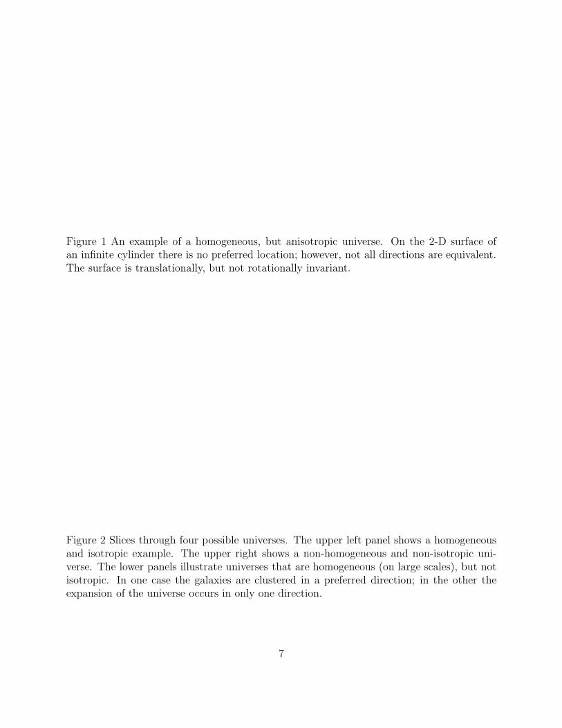
Figure 1 An example of a homogeneous, but anisotropic universe. On the 2-D surface ofan infinite cylinder there is no preferred location; however, not all directions are equivalent.The surface is translationally, but not rotationally invariant.

Figure 2 Slices through four possible universes. The upper left panel shows a homogeneousand isotropic example. The upper right shows a non-homogeneous and non-isotropic uni-verse. The lower panels illustrate universes that are homogeneous (on large scales), but notisotropic. In one case the galaxies are clustered in a preferred direction; in the other theexpansion of the universe occurs in only one direction.

7

of the Universe. As we have seen above, the geometry, dynamics, and matter distribution ofa universe can be arbitrarily complex. In the absence of any knowledge of these quantities,where should we begin?

The most logical approach is the spherical cow approach – start with the simplest physicalsystem, adding complexity only when required. Towards this end, Albert Einstein introducedwhat is known as the Cosmological Principle. The Cosmological Principle states thatthe Universe is homogeneous and isotropic.

It is immediately obvious that this principle is incorrect on small scales – this classroomfor instance is clearly not homogeneous and isotropic. Similarly, there are obvious inhomo-geneities on galaxy, galaxy cluster, and even supercluster scales. However, if you averageover larger scales, then the distribution of matter is indeed approximately uniform. TheCosmological Principle should therefore be thought of as a reasonable approximation of theUniverse on large scales – specifically scales much greater than the size of gravitationallycollapsed structures. Both the global homogeneity and isotropy (at least from our perspec-tive) have been remarkable confirmed by observations such as cosmic microwave backgroundexperiments (COBE, WMAP) and large galaxy redshift surveys. The success of the Cos-mological Principle is remarkable given that it was proposed at time with the existence ofexternal galaxies was still a subject of debate.

2.2.1 Spatial Invariance of Physical Laws

If we ponder the implications of the Cosmological Principle, we see that it has importantphysical consequences. Perhaps the most fundamental implication of accepting the Cos-mological Principle is that the known laws of physics, derived locally, must remain valideverywhere else in the Universe. Otherwise the assumption of homogeneity would be vio-lated. Reassuringly, modern observations appear to validate this assumption, at least withinthe observable universe, with the properties of distant astrophysical objects being consistentwith those observed locally. Within our own Galaxy, period changes for binary pulsars areconsistent with the slowdown predicted by General Relativity as a result of gravitationalradiation. On a much more distant scale, the light curves of type Ia supernovae are similarin all directions out to z ≈ 1 (d ∼ 8 billion light years), and have the same functional formas those at z = 0. Indeed, terrestrial physics has been remarkably successful in explainingastrophysical phenomena, and the absence of failures is a powerful argument for spatial in-variance. As an aside, it is worth nothing that dark matter and dark energy, which we willdiscuss later, are two instances in which standard physics cannot yet adequately describe theuniverse. Neither of these phenomena violate spatial invariance though – they’re a problemeverywhere.

2.2.2 The Copernican Principle

Additionally, the Cosmological Principle has a philosophical implication for the place ofmankind in the Universe. The assumption of isotropy explicitly requires that we are not ina preferred location in the Universe, unlike the center of the 3-D sphere discussed above.

8

The Cosmological Principle therefore extends Copernicus’ displacement of the Earth fromthe center of the solar system. The statement that we are not in a preferred location issometimes called the Copernican Principle.

2.2.3 The Perfect Cosmological Principle

It is worth noting that there exists a stronger version of the Cosmological Principle calledthe “Perfect Cosmological Principle”. The Perfect Cosmological Principle requires thatthe Universe also be the same at all times, and led rise to the “steady-state” cosmology(Hoyle 1948), in which continuous creation of matter and stars maintained the density andluminosity of the expanding Universe. We now know that the Universe is not infinitely old(and could have from Olbers’ paradox!), yet this can still be considered relevant in largercontexts such as eternal inflation, where our Universe is one of an infinite number. In thiscase we may have a preferred time in our own Universe, but the Universe itself is not at apreferred “time”.

2.2.4 Olbers’ Paradox Revisited

Finally, it is worth taking one last look at Olbers’ Paradox in light of the CosmologicalPrinciple. Of the five assumptions listed before, the first and fifth are simply implications ofthe cosmological principle. Since we showed that the fourth was unnecessary, we return tothe conclusion that either 2. or 3. must be false.

2.3 Expansion and the Cosmological Principle

One of the most influential observations of the 20th century was the discovery by EdwinHubble of the expansion of the Universe (Hubble 1929). Hubble’s law states that the reces-sional velocity of external galaxies is linearly related to their distance. Specifically, v = H0d,where v is velocity, d is the distance of a galaxy from us, and H0 is the “Hubble constant”. [Itturns out that this “constant” actually isn’t, and the relation is only linear on small scales,but we’ll get to this later.].

It is straightforward to derive Hubble’s law as a natural consequence of the Cosmologi-cal Principle. Consider a triangle, sufficiently small that both Euclidean geometry is a validapproximation (even in a universe with curved geometry) and v << c so that Galilean trans-formations are valid. As the universe expands or contracts, the conditions of homogeneityand isotropy require that the expansion is identical in all locations. Consequently, the tri-angle must grow self-similarly. If we define the present time at t0 and the scale factor of theexpansion as a(t), with a0 = a(t0) being the scale factor at t0, then this self-similarity requiresthat any distance x increase by the same scale factor. Mathematically, this is equivalent tosaying that

x =(

a

a0

)

x0. (11)

9

Taking the derivative,

x =(

a

a0

)

x0 =(

a

a

)

x, (12)

orv = Hx, (13)

where the Hubble parameter is defined as H ≡ a/a. The Hubble constant, H0 is definedat the value of the Hubble parameter at t0, i.e. H0 = a0/a0. Note that the CosmologicalPrinciple does not require H > 0 – it is perfectly acceptable to have a static or contractinguniverse.

3 Dynamics of the Universe - Conservation Laws, Fried-

mann Equations

To solve for the dynamics of the universe, it is necessary to use the Cosmological Principle(or another symmetry principle) along with General Relativity (or another theory of grav-ity). In this lecture we shall use a Newtonian approximation to derive the evolution of theuniverse. The meaning of these solutions within the framework of GR will then be discussedto illustrate the effect of spatial curvature and the behavior of light as it propagates. It turnsout that the trajectory of light cannot be treated self-consistently within the framework ofNewtonian gravity – essentially because of the need for Lorentzian rather than Galileaninvariance for relativistic velocities.

As a reminder, for Galilean transformation,

x′ = x− vt (14)

t′ = t, (15)

while for a Lorentz transformation

x′ =x− vt

√

1− (v/c)2(16)

t′ =t− vx

c2√

1− (v/c)2. (17)

3.1 Conservation Laws in the Universe

Let us approximate a region of the universe as a uniform density sphere of non-relativisticmatter. We will now use the Eulerian equations for conservation of mass and momentum toderive the dynamical evolution of the universe.

10

3.1.1 Conservation of Mass

If we assume that mass is conserved, then the mass density ρ satisfies the continuity equation

∂ρ

∂t= ∇ · (vρ) = 0. (18)

The Cosmological Principle demands that the density ρ be independent of position. Usingthe fact that ∇ · v = 3H(t), the continuity equation becomes

dρ

dt+ 3H(t)ρ = 0, (19)

ordρ

ρ= −3H(t)dt, (20)

which integrates to

ln

(

ρ

ρ0

)

= −3∫ t

t0dtH(t) = −3

∫ a

a0

da

a= −3 ln

(

a

a0

)

. (21)

This can be rewritten as

ρ(t) = ρ0

(

a0

a

)3

, (22)

so the time dependence is determined solely by the evolution of the scale factor and for amatter dominated universe ρ ∝ a−3. This intuitively makes sense, as it’s equivalent to sayingthat the matter density is inversely proportional to the volume.

3.1.2 Conservation of Momentum

We would like to apply conservation of momentum to the Universe using Newton’s theory ofgravity. This approach would seem, at first glance, to be inconsistent with the CosmologicalPrinciple. Euler’s equation for momentum conservation is

∂ρv

∂t+∇ · (ρv)v +∇p = Fρ, (23)

where v is the local fluid velocity with respect to a co-comoving observer, p is the pressure,and F is the force (in this case gravitational) per unit mass. An immediate problem is thatit is difficult to define the gravitational potential in a uniform unbounded medium. We couldapply Newton’s laws to a universe which is the interior of a large sphere. This violates theCosmological Principle since we sacrifice isotropy; however it doesn’t violate it too badly if weconsider only regions with size x << Rsphere. In fact, Milne & McCrea (1934) demonstratedthat Newtonian cosmology is a reasonable approximation to GR. In that spirit, we shall useEuler’s equations in an unbounded medium to represent conservation of momentum.

11

The above version of Euler’s equation makes the physical meaning of each term apparent,but let us now switch to the more commonly used form,

∂v

∂t+ (v · ∇)v = F− ∇p

ρ. (24)

The Cosmological Principle requires that the pressure gradient must be zero, and usingthe fact that x · ∇x = x, the equation becomes

x[

H +H2]

= F. (25)

Poisson’s equation for the gravitational force is

∇ · F = −4πGρ. (26)

Taking the divergence of both sides above, and using ∇ · x = 3, we get

dH

dt+H2 = −4πGρ/3. (27)

Using

H(t) =a

a, (28)

along with mass conservation, this can be converted into an equation for the scale factor.

a

a−(

a

a

)2

+(

a

a

)2

= −4πGρ

3, (29)

which simplifies to

a = −4πGρ

3a, (30)

or, using our result for the evolution of the matter density,

a2a = −4πGρ0a30

3. (31)

This is the basic differential equation for the time evolution of the scale factor. It is alsothe equation for the radius of a spherical self-gravitating ball.

Looking at the equation, it is clear that the only case in which a = 0 is when ρ0 = 0 –an empty universe. [We will revisit this with the more general form from GR, but this basicresult is OK.] To obtain a static universe, Einstein modified GR, to give it the most generalform possible. His modification was to add a constant (for which there is no justification inNewtonian gravity), corresponding to a modification of Poisson’s Law,

∇ · F = −4πGρ+ Λ, (32)

12

where Λ is referred to as the cosmological constant. The cosmological constant Λ must havedimensions of t−2 to match the units of ∇ · F If |Λ| ∼ H2

0 , it would have virtually no effecton gravity in the solar system, but would affect the large-scale universe.

If we include Λ, our previous derivation is modified such that

3(H +H2) = −4πGρ+ Λ (33)

a

a= −4πGρ

3+

Λ

3, (34)

or equivalently

a = (−4πGρ

3+

Λ

3)a = −4πGρ0a

30

3a−2 +

Λ

3a, (35)

Note that a positive Λ corresponds to a repulsive force than can counteract gravity. Wenow multiply both sides by a and integrate with respect to dt:

1

2a2 =

4πGρ0a30

3

1

a+

Λ

3

a2

2+K, (36)

ora2

a2=

8πGρ0

3

a0

a

3

+Λ

3+Ka−2, (37)

where K is an arbitrary constant of integration. For the case of a self-gravitation sphere withΛ = 0, K/2 is just the total energy per unity mass (kinetic plus potential) at the surface ofthe sphere. In GR, we shall see that K is associated with the spatial curvature. The aboveequation describes what are called the Friedmann solutions for the scale factor of theuniverse. It implicitly assumes that the universe is filled with zero pressure, non-relativisticmaterial (also known as the dust-filled model).

The above equations give some intuition for the evolution of the scale factor of the uni-verse. The equation shows that for an expanding universe, where a(0) = 0, the gravitationalterm should dominate for early times when a is small. As the universe expands though, firstthe curvature term and later the cosmological constant term are expected to dominate theright hand side of the equation.

Let us now introduce one additional non-Newtonian tweak to the equations. The aboveequations correspond to a limiting case of the fully correct equations from GR in which thepressure is zero and the energy density is dominated by the rest mass of the particles. Tobe fully general, the matter density term should be replaced by an “effective density”

ρeff = ρ+3p

c2, (38)

where ρ should now be understood to be the total energy density (kinetic + rest mass).With this modification, Equation 34 becomes

a

a= −4πG

3

(

ρ+3p

c2

)

+Λ

3. (39)

13

It is worth emphasizing at this point that the energy density ρ will include contributionsfrom both matter and radiation, which as we shall see have different dependences upon thescale factor.

Finally, we can now re-obtain the equation above for the first derivative if we take intoaccount that the expansion of the universe with be adiabatic, i.e.

dE = −pdV → d(ρc2a3) = −pda3. (40)

This equation can be rewritten

a3d(ρc2) + (ρc2)da3 = −pda3, (41)

(ρc2 + p)da3 + a3d(ρc2 + p) = a3dp (42)

d[

a3(ρc2 + p)]

= a3dp (43)

pa3 =d

dt

[

a3(ρc2 + p)]

(44)

which yields

ρ+ 3(

ρ+p

c2

)

a

a= 0. (45)

If we now return to deriving the equation for the first derivative,

a

a= −4πG

3

(

ρ+3p

c2

)

+Λ

3, (46)

1

2

da2

dt= −4πG

3

(

ρ+3p

c2

)

aa +Λ

3aa. (47)

The expression for adiabatic expansion can be rewritten,

3p

c2a

a= −ρ− 3ρ

a

a, (48)

which can be inserted to yield

1

2

da2

dt= −4πG

3

(

ρaa− ρa2 − 3ρaa)

+Λ

3aa, (49)

1

2

da2

dt=

4πG

3

(

2ρaa + ρa2)

+Λ

3aa, (50)

1

2

da2

dt=

4πG

3

dρa2

dt+

Λ

6

d

dta2, (51)

and hence

a2 =8πGρa2

3+

Λa2

3− k. (52)

In the context of GR, we will come to associate the constant k with the spatial curvatureof the universe. GR is fundamentally a geometric theory in which gravity is described as acurved spacetime rather than a force. In this Newtonian analogy the quantity -k/2 wouldbe interpreted as the energy per unit mass for a particle at the point a(t) in the expandingsystem.

14

3.2 Conclusions

The two Friedmann equations,

a

a= −4πG

3

(

ρ+3p

c2

)

+Λ

3, (53)

a2 =8πGρa2

3+

Λa2

3− k, (54)

together fully describe the time evolution of the scale factor of the universe and will be usedextensively during the next few weeks.

3.3 An Example Solution and Definitions of Observable Quanti-

ties

Let us now work through one possible solution to the Friedmann equations. For a simplecase, we will start with Λ = 0. At the present

(

da

dt

)

t=to

= a0 = a0H0. (55)

We can now evaluate the constant k in terms of observable present day quantities.

a2 =8πGρa2

3− k, (56)

a20 ≡ H2

0a20 =

8πGρ0a20

3− k, (57)

k = −a20

[

8πGρ0

3−H2

0

]

=8πG

3a2

0

(

ρ0 −3H2

0

8πG

)

. (58)

Clearly, k = 0 only if ρ0 is equal to what we will define as the critical density,

ρcrit =3H2

0

8πG. (59)

With this definition,

k =8πG

3a2

0ρ0

(

ρ0

ρcrit− 1

)

= −8πG

3a2

0ρ0 (Ω0 − 1) , (60)

where we have further defined,

Ω0 ≡ρ0

ρcrit=

8πGρ0

3H20

. (61)

15

Note that this has the corollary definition

H20 =

8πGρ0

3Ω0. (62)

Inserting the definition for the curvature back into the Friedmann equation, we see that

a2 =8πGρ0

3

a30

a+

8πGa20ρcrit

3(1− Ω0), (63)

or

(

a

a0

)2

=Ω0H

20a0

a+

8πGρcrit3

(1− Ω0) (64)

(

a

a0

)2

=Ω0H

20a0

a+H2

0 (1− Ω0) (65)

We now consider big bang solutions, i.e. a(0) = 0. At very early times (a ∼ 0), thefirst term on the rhs – the gravitational term, will dominate the second term. Thus, atearly times the form of the solution should be independent of the density. However, at latertimes the nature of the solution depends critically upon whether the second (energy) termis positive, negative, or zero. Equivalently, it depends whether Ω0 is less than, equal to, orgreater than 1. If Ω0 < 1 and the energy term is positive, the solution for a(t) is analogousto the trajectory of a rocket launched with a velocity greater than the escape velocity.

Consider now the case Ω0 = 1, which is called the Einstein-deSitter universe. This casemust always be a good approximation at early time. Then

da

dt=H0a

3/20

a1/2, (66)

a1/2da = H0a3/20 dt (67)

or, assuming a(0) = 0,

a

a0=(

3H0t

2

)2/3

. (68)

Thus, a(t) is a very simple function for the Einstein-deSitter case. We can also veryeasily solve for the age of the universe,

t0 =2

3H−1

0 . (69)

Indeed, H−10 overestimates the age of the universe for all Friedmann models with Λ = 0.

Now consider the case of Ω0 > 1. The maximum scale factor amax occurs when a = 0 inequation 65,

amaxa0

=Ω0

Ω0 − 1. (70)

16

We can obtain a parametric solution by letting

a(t) = amax sin2 θ =Ω0a0

Ω0 − 1sin2θ. (71)

Substituting this into equation 65 gives

(

Ω0

Ω0 − 1

)2

4 sin2 θ cos2 θ θ2 = H20 (Ω0 − 1)

cos2 θ

sin2 θ, (72)

H0t =2Ω0

(Ω0 − 1)3/2

∫ θ

0dx sin2 x =

Ω0

(Ω0 − 1)3/2

[

θ − 1

2sin 2θ

]

. (73)

The above equation represents a parametric solution for the scale factor when Ω0 > 1.Since the lifetime of the universe extends from θ = 0 to θ = π, the total lifetime of theuniverse is

tlifetime =πΩ0

H0 (Ω0 − 1)3/2(74)

A similar parametric solution for H0t can be derived for Ω0 < 1 by replacing sin θ with sinh θin the expression for a(t). In this case, a(t) ∝ t for large t.

3.4 The Friedmann Equations from General Relativity

Before moving on to a discussion of spacetime metrics, it is worth at least briefly mentioningthe origin of the Friedmann equations in the context of General Relativity. They are deriveddirectly from Einstein’s field equations,

Gij ≡ Rij −1

2Rgij =

8πG

c4Tij , (75)

or, including the cosmological constant,

Rij −1

2Rgij − Λgij =

8πG

c4Tij (76)

The gik comprise the metric tensor, describing the metric of spacetime. T is the energy-momentum tensor, and encapsulates all the information about the energy and momentumconservation laws that we discussed in the Newtonian context. The conservation law in thiscontext is simply T ji;j = 0, which means that the covariant derivative is zero. The Riccitensor (Rij) and Ricci scalar (R) together make up the Einstein tensor.

In cosmology, the energy-momentum tensor of greatest relevance is a perfect fluid,

Tij = (ρc2 + p)UiUj − pgij (77)

where Uk is the fluid four-velocity. Remember that we assumed a perfect fluid in the New-tonian analog. This covariant derivative of the tensor provides the analog to the Eulerequations. Substituting this expression for the stress tensor yields, after some math, theFriedmann equations.

17

4 Spacetime Metrics

It is important to interpret the solutions for the scale factor obtained from Newtonian theoryin the last section within the framework of GR. While Newtonian theory treats gravity as aforce, in GR the presence of a mass is treated as curving or warping spacetime so that it isno longer Euclidean. Particles moving under the influence of gravity travel along geodesics,the shortest distance between two points in curved spacetime. It is therefore necessary tobe able to describe spatial curvature in a well-defined way.

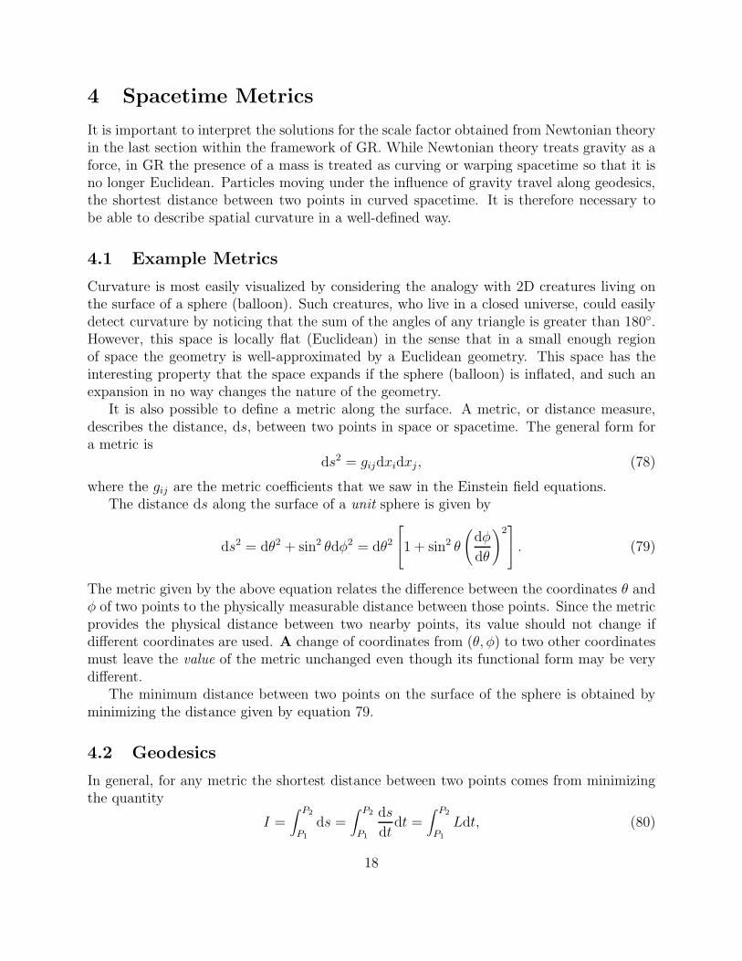
4.1 Example Metrics

Curvature is most easily visualized by considering the analogy with 2D creatures living onthe surface of a sphere (balloon). Such creatures, who live in a closed universe, could easilydetect curvature by noticing that the sum of the angles of any triangle is greater than 180.However, this space is locally flat (Euclidean) in the sense that in a small enough regionof space the geometry is well-approximated by a Euclidean geometry. This space has theinteresting property that the space expands if the sphere (balloon) is inflated, and such anexpansion in no way changes the nature of the geometry.

It is also possible to define a metric along the surface. A metric, or distance measure,describes the distance, ds, between two points in space or spacetime. The general form fora metric is

ds2 = gijdxidxj , (78)

where the gij are the metric coefficients that we saw in the Einstein field equations.The distance ds along the surface of a unit sphere is given by

ds2 = dθ2 + sin2 θdφ2 = dθ2

1 + sin2 θ

(

dφ

dθ

)2

. (79)

The metric given by the above equation relates the difference between the coordinates θ andφ of two points to the physically measurable distance between those points. Since the metricprovides the physical distance between two nearby points, its value should not change ifdifferent coordinates are used. A change of coordinates from (θ, φ) to two other coordinatesmust leave the value of the metric unchanged even though its functional form may be verydifferent.

The minimum distance between two points on the surface of the sphere is obtained byminimizing the distance given by equation 79.

4.2 Geodesics

In general, for any metric the shortest distance between two points comes from minimizingthe quantity

I =∫ P2

P1

ds =∫ P2

P1

ds

dtdt =

∫ P2

P1

Ldt, (80)

18

where the two points P1 and P2 are held fixed, t is a dummy variable that varies continuouslyalong a trajectory, and the Lagrangian L = ds/dt. Minimization of the Lagrangian yieldsthe equation of motion in special relativity.

If P1 and P2 are held fixed then the integral is minimized when Lagrange’s equationsare satisfied (same as in classical mechanics),

∂L

∂xi=

d

dt

∂L

∂xi, i = 1..N. (81)

Consider the example of the shortest distance (geodesic) between two points on thesurface of a unit sphere. Let the independent variable be θ instead of t. Then the Lagrangianis

L ≡ ds

dθ=

√

√

√

√1 + sin2 θ

(

dφ

dθ

)2

, (82)

and Lagrange’s equation is

∂L

∂φ=

d

dθ

∂L

∂φ, (83)

d

dθ

sin2 θ φ√

1 + sin2 θφ2

= 0, (84)

where φ = dφ/dθ.Integrating and squaring this equation gives

sin4 θ

[

d

dθ(φ− C2)

]2

= C1

1 + sin2 θ

[

d

dθ(φ− C2)

]2

. (85)

Let y = φ− C2 and x = cot θ. Then dxdθ

= −1sin2θ

and the differential equation becomes

(

dy

dx

)2

= C1

(1− y2) + (1 + x2)

(

dy

dx

)2

, (86)

with the solution

y =(

C1

1− C1

)1/2

x = C ′1x, (87)

or,cos(φ− C2) = C ′

1 cot θ. (88)

The above equation gives the geodesics along the surface of a sphere. But this is just theexpression for a great circle! To see this, consider that a plane through the origin,

x+ Ay +Bz = 0 (89)

19

produces the following locus of intersection with a unit sphere:

sin θ cosφ+ A sin θ sinφ+B cos θ = 0, (90)

B + tan θ(A sin φ+ cos φ) = 0, (91)

−B cot θ = C cos(φ−D). (92)

Therefore we have demonstrated that geodesics on the surface of a sphere are great circles.Of course, this can be proven much more easily, but the above derivation illustrates thegeneral method for determining geodesics for an arbitrary metric.

4.3 Special Relativity and Curvature

Week 3 Reading Assignment: Chapter 2For special relativity, in a Lorentz frame we can define a distance in spacetime as

ds2 = c2dt2 − dx2 = c2dt2(

1− v2

c2

)

. (93)

This metric also relates physically measurable distances to differences in coordinates. Forexample, the time measured by a moving clock (the proper time) is given by ds/c. Thus,proper time intervals are proportional to, but not equal to, dt.

Let’s look at the above metric for a moment. For light, the metric clearly yields ds2 = 0.Light is therefore said to follow a null geodesic, which simply means that the physical distancetravelled is equal to ct. Everything that we see in the universe by definition lies along nullgeodesics, as the light has just had enough time to reach us. Consider Figure 3. The nullgeodesics divide the spacetime plane into two types of world lines. World lines with ds2 > 0are said to be timelike because the time component is larger. Physically, this means thatwe observed (received the light from) events with timelike world lines some time in the past.World lines with ds2 < 0 are said to be spacelike. Spacetime points that lie along spacelikeworld lines are sufficiently far that light has not yet had time to reach us.

Now, consider the equation of motion for a particle in special relativity. For a freeparticle, the equation of motion follows from minimizing the distance between two fixedpoints in space time, analogous to the case with the surface of the sphere,

δ∫ 2

1ds = δ

∫ t2

t1Ldt = 0. (94)

Since the Lagrangian is

L = c

[

1−(

v

c

)2]1/2

= c

(

1− v2

2c2+ ...

)

, (95)

and since the first term is constant, for nonrelativistic free particles (v << c) the specialrelativistic Lagrangian reduces to the usual nonrelativistic Lagrangian without interactions.

20

Figure 3 Light cones for a flat geometry. Light travels along the null geodesics, while particlestravel along timelike geodesics. Points with ds2 < 0 are not observable at the present time..

Note that in the case of external forces, the situation is not quite so simple. Recall thatthe classical Lagrangian is given by

L =1

2mv2 − U. (96)

The analog in special relativity is

L = −mc2√

1− v2/c2 − U, (97)

If one wishes to calculate the motion of a relativistic particle undergoing electromagneticinteractions, then one must include the electrostatic potential Φ and the vector potential Ain the Lagrangian as

U = eΦ− e

cv ·A. (98)

In general relativity, gravity is treated as an entity that modifies the geometry of space-time. Particles travel along geodesics in that geometry with the equation of motion

δ∫ 2

1ds = 0. (99)

Thus, gravitational forces, as such, do not exist. The presence of massive bodies simplyaffects the geometry of spacetime. When spacetime is curved due to the presence of gravi-tational mass, particles no longer travel on straight lines in that geometry. If one wishes to

21

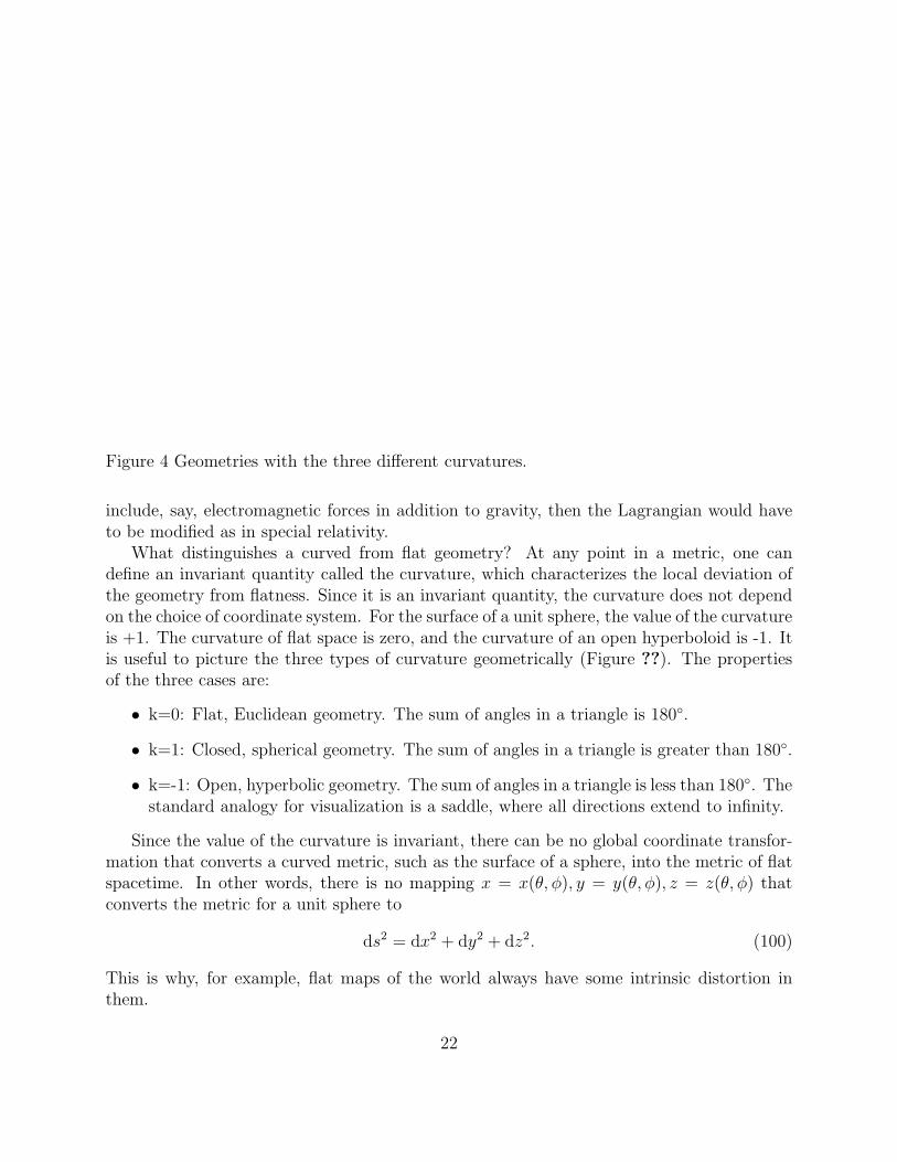
Figure 4 Geometries with the three different curvatures.

include, say, electromagnetic forces in addition to gravity, then the Lagrangian would haveto be modified as in special relativity.

What distinguishes a curved from flat geometry? At any point in a metric, one candefine an invariant quantity called the curvature, which characterizes the local deviation ofthe geometry from flatness. Since it is an invariant quantity, the curvature does not dependon the choice of coordinate system. For the surface of a unit sphere, the value of the curvatureis +1. The curvature of flat space is zero, and the curvature of an open hyperboloid is -1. Itis useful to picture the three types of curvature geometrically (Figure ??). The propertiesof the three cases are:

• k=0: Flat, Euclidean geometry. The sum of angles in a triangle is 180.

• k=1: Closed, spherical geometry. The sum of angles in a triangle is greater than 180.

• k=-1: Open, hyperbolic geometry. The sum of angles in a triangle is less than 180. Thestandard analogy for visualization is a saddle, where all directions extend to infinity.

Since the value of the curvature is invariant, there can be no global coordinate transfor-mation that converts a curved metric, such as the surface of a sphere, into the metric of flatspacetime. In other words, there is no mapping x = x(θ, φ), y = y(θ, φ), z = z(θ, φ) thatconverts the metric for a unit sphere to

ds2 = dx2 + dy2 + dz2. (100)

This is why, for example, flat maps of the world always have some intrinsic distortion inthem.

22

Similarly, there is no coordinate transformation that converts the metric of special rela-tivity (called the Minkowski metric)

ds2 = c2dt2 − dx2 (101)

into a curved geometry.

4.4 The Robertson-Walker Metric

We have looked at examples of metrics for a unit sphere and for special relativity. Letus now turn our attention to the question of whether we can construct a metric that isvalid in a cosmological context. Assume that (1) the cosmological principle is true, and (2)each point in spacetime has one and only one co-moving, timelike geodesic passing throughit. Assumption (2) is equivalent to assuming the existence of worldwide simultaneity oruniversal time. Then for a co-moving observer, there is a metric for the universe called theRobertson-Walker metric, or sometimes the Friedmann-LeMaitre-Robertson-Walker metric(named after the people who originally derived it). The Robertson-Walker metric is

ds2 = (c dt)2 − a(t)2

[

dr2

1− kr2+ r2dη2

]

, (102)

where k is the sign of the curvature (k = −1, 0, 1), a(t) is the scale factor, and r is theco-moving distance. The dη term is short-hand for the solid angle,

dη2 = sin2 θdφ2 + dθ2. (103)

For a given curvature, this metric completely specifies the geometry of the universe towithin one undetermined factor, a(t), which is determined from the Friedmann equations.Together, the Friedmann equations and Robertson-Walker metric completely describe thegeometry.

The above form of the metric is the one given in the text; however, there are in fact threecommonly used forms for the metric,

ds2 = (c dt)2 − a(t)2

dr2 +

(

sin kr

k

)2

dη2

, (104)

ds2 = (c dt)2 − a(t)2

(1 + 14kr2)2

[

dr2 + r2dη2]

, (105)

ds2 = (c dt)2 − a(t)2

[

dr2

1− kr2+ r2dη2

]

. (106)

All three forms are equivalent, yielding the same value for the distance between two points.Transformation between the forms is possible given the appropriate variable substitutions.These transformations are left as a homework exercise.

23

In the above equations, k is the same curvature that we discussed in the context ofspecial relativity. The phrases “open” and “closed” now take on added significance in thesense that, for Λ = 0, a “closed” will recollapse while an “open” universe will expand forever.In contrast, the recent discovery that Λ 6= 0 has given rise to the phrase: “Geometry is notdestiny”. In the presence of a cosmological constant, the strict relation above does not hold.

4.4.1 Proper and Co-moving Distance

Given the above metric, we will be able to measure distances. Looking at the equation, letus start with two distance definitions

• Proper Distance: Proper distance is defined as the actual spatial distance betweentwo co-moving observers. This distance is what you would actually measure, and is afunction of time as the universe expands.

• Co-moving (or coordinate) distance: The co-moving distance is defined such thatthe distance between two co-moving observers is independent of time. The standardpractice is to define the co-moving distance at the present time t0.

As an illustration, consider two co-moving observers currently separated by a properdistance r0. At any lookback time t, the proper separation will be

DP = (a/a0)r0, (107)

while the co-moving distance will beDC = r0. (108)

Note that it is a common practice to set a0 = 1.

4.4.2 Derivation of the Robertson-Walker Metric

We shall now derive the Robertson-Walker metric. While the metric can be derived byseveral methods, we will go with a geometric approach for clarity. Consider an arbitraryevent (t, r) in spacetime. This event must lie within a spacelike 3D hypersurface withinwhich the universe everywhere appears identical to its appearance at the point in question(homogeneity). The set of co-moving timelike geodesics (world lines of co-moving observers)through each point on this hypersurface defines the universal time axis. The metric can thenbe expressed in the form

ds2 = c2dt2 − dχ2, (109)

where dχ is the distance measured within the spacelike hypersurface. There are no crossterms dχdt because the time axis must be perpendicular to the hypersurface. Otherwise thereis a largest cross-term that yields a preferred spacelike direction, thus violating isotropy. Ifwe choose a polar coordinate system, then dχ2 can be written in the form

dχ2 = Q(r, t)[

dr2 + r2dη2]

, (110)

24

where Q(r, t) includes both the time and spatial dependence. Again by isotropy, all crossterms like drdη must vanish. The second term inside the brackets can have a differentcoefficient than the first term, but we have the freedom to define r so that the coefficientsare the same.

The proper distance δx between two radial points r and r + δr is

δx = Q1/2δr. (111)

Locally, geometry is Euclidean, and local Galilean invariance implies that Hubble’s law isvalid:

H(t) =1

δx

∂

∂tδx =

1

2Q

∂Q

∂t(112)

Hubble’s law must be independent of position, r, because of the Cosmological Principle.Therefore Q(r, t) must be separable,

Q(r, t) = a2(t)G(r), (113)

so the metric isds2 = c2dt2 − a2(t)G(r)

[

dr2 + r2dη2]

. (114)

Let us now transform the radial coordinates to

dχ2 = dr2 + F 2(r)dη2 (115)

using the change of variables

F (r) = G(r)r, (116)

dr = G(r)dr. (117)

For a Euclidean geometry,dχ2 = dr2 + dη2, (118)

so F (r) = r in the Euclidean case. Since spacetime locally appears Euclidean, we thereforerequire in the limit (r → 0) that F (0) = 0 and F ′(0) =1.

Now consider the triangles below.If the angles α, β, γ are small, and if x, y, z are proper distances, we get 3 identities:

F (r)α = F (ǫ+ τ)γ, (119)

F (r + ǫ+ τ)α = F (ǫ+ τ)β, (120)

F (r + ǫ)α = F (ǫ)β + F (τ)γ. (121)

Eliminating β and γ from the three equations, we get

F (r + ǫ) = F (ǫ)F (r + ǫ+ τ)

F (ǫ+ τ)+ F (τ)

F (r)

F (ǫ+ τ), (122)

F (ǫ+ τ)F (r + ǫ) = F (ǫ)F (r + ǫ+ τ) + F (τ)F (r). (123)

25

Figure 5 Geometric Derivation of Robertson-Walker Metric

Take the limit ǫ→ 0 and expand to first order in ǫ.

[F (τ) + ǫF ′(τ)] [F (r) + ǫF ′(r)] = ǫF (r + τ) + F (τ)F (r)), (124)

F (τ)F (r) + ǫF (τ)F ′(r) + ǫF ′(τ)F (r) + ǫ2F ′(τ)F ′(r) = ǫF (r + τ) + F (τ)F (r)), (125)

F (r)F ′(τ) + F (τ)F ′(r) = F (r + τ). (126)

Expand to second order in τ :

F (r)[

1 + τF ′′(0) +1

2τ 2F ′′′(0)

]

+F ′(r)[

F (0) + τF ′(0) + +1

2τ 2F ′′(0)

]

= F (r)+τF ′(r)+1

2τ 2F ′′(r),

(127)or, using the limits for F (0) and F ′(0), the first order terms give

F ′′(0) = 0, (128)

and the second order terms give

F ′′(r) = F ′′′(0)F (r). (129)

Define k ≡ (−F ′′′(0))1/2. Then

F ′′(r) = −k2F (r), (130)

and this has the general solution

F (r) = A sin(kr +B). (131)

26

From the boundary conditions, F (0) = 0 implies B = 0, and F ′(0) = 1 implies kA = 1.Therefore, the solution is

F (r) =sin kr

k. (132)

Verify the third derivative:F ′′′(0) = −k2 cos 0 = −k2. (133)

Correct. The sign of k determines the nature of the solution:

• k = 1→ F (r) = sin r

• k = 0→ F (r) = r

• k = −1→ F (r) = sinh r.

Thus, we have the Robertson-Walker metric,

ds2 = (c dt)2 − a(t)2

dr2 +

(

sin kr

k

)2

dη2

, (134)

which can be converted to the other standard forms.

5 Redshift

OK. Stepping back for a second, we now have a means of describing the evolution of thesize of the universe (Friedmann equation) and of measuring distances within the universe(Robertson-Walker metric). It’s time to recast these items in terms of observable quantitiesand use this machinery to develop a more concise description our Universe. We don’t directlyobserve the scale factor, a(t), but we can observe the cosmological redshift of objects dueto the expansion of the universe. As you may recall, the Doppler shift of light (redshift orblueshift) is defined as

z =λo − λeλe

=νe − νoνo

, (135)

where λo and λe are the observed and emitted wavelengths, and νo and νe are the corre-sponding frequencies. This can be recast in terms of frequency as

1 + z =νeνo. (136)

We know that light travels along null geodesics (ds = 0). Therefore, for light travellingto us (i.e. along the radial direction) the RW metric implies

c2dt2 = a2 dr2

1− kr2(137)

cdt

a=

dr

1− kr2= f(r). (138)

27

Consider two photons at distance R, emitted at times te and te + δte, that are observed attimes to and to + δto. Since both are emitted at distance R, f(r) is the same and

∫ to

t1

cdt

a=∫ to+δto

te+δte

cdt

a. (139)

If δte is small, then the above equation becomes

δtoao

=δt1ae

(140)

νoao = νeae (141)νeνo

=aoae

= 1 + z, (142)

where the last relation comes from the definition of redshift. Taking ao to be now (t0), anddefining a0 ≡ 1 we therefore have the final relation

a =1

1 + z. (143)

Note that there is a one-to-one correspondence between redshift and scale factor – andhence also time. The variables z,a, and t are therefore interchangeable. From this point on,we will work in terms of redshift since this is an observable quantity. We do, however, needto be aware that the cosmological expansion is not the only source of redshift. The othersources are

• Gravitational redshift: Light emitted from deep within a gravitational potential wellwill be redshifted as it escapes. This effect can be the dominant source of redshift insome cases, such as light emitted from near the event horizon of a black hole.

• Peculiar velocities: Any motion relative to the uniform expansion will also yield aDoppler shift. Galaxies (and stars for that matter) do not move uniformly with theexpansion, but rather have peculiar velocities relative to the Hubble flow of severalhundred km s−1 – or even > 1000 km s−1 for galaxies in clusters. In fact, some of thenearest galaxies to us are blueshifted rather than redshifted. This motion, which isa natural consequence of gravitational attraction, dominates the observed redshift fornearby galaxies.

The total observed redshift for all three sources is

(1 + z) = (1 + zcosmological)(1 + zgrav)(1 + zpec). (144)

Also, between two points at redshifts z1 and z2 (z1 being larger), the relative redshift is

1 + z12 =1 + z11 + z2

=a1

a2. (145)

28

6 The Friedmann Equations 1: Observable Quantities

Recall again the Friedmann equation,

a2 + kc2 =8πG

3ρa2 +

Λc2

3a2. (146)

We will now recast this in a simpler form corresponding to observable quantities. First,let us list and define these quantities.

6.1 The Hubble parameter (H)

We have previously defined the Hubble parameter as

H =a

a(147)

and the Hubble constant as

H0 =a0

a0. (148)

7 The density parameter (Ω0)

We have previously defined the density parameter as the ratio of the actual density to thecritical density at the current time (t0). The critical density ρc is the density required tojust halt the expansion of the universe for models with Λ = 0, and is given by

ρc =3H2

0

8πG. (149)

The matter density parameter at the current time is thus,

Ω0 =ρ0

ρc=

8πGρ0

3H20

. (150)

8 The cosmological constant density parameter (Ω0Λ)

Consider a empty universe (Ω0 = 0). The “critical” value of the cosmological constant isdefined as the value required for a flat universe in this model (k = 0). Specifically, for timet0 the Friedmann equation above becomes

a20

a20

− Λcc2

3= 0 (151)

Λc =3H2

0

c2. (152)

29

The parameter ΩΛ is defined as

ΩΛ =Λ

Λc=

Λc2

3H20

. (153)

This is basically a statement describing the contribution of the energy density in the cosmo-logical constant as a fraction of the total required to close the universe.

9 The Observable Friedmann Equation

Using the above equations, let’s now proceed to recast the Friedmann equation.

a2 + kc2 =8πG

3ρa2 +

Λc2

3a2 (154)

= a2

[

8πGρ0

3H20

ρ

ρ0

H20 +

Λc2

3H20

H20

]

(155)

a2 = a2H20

[

Ω0ρ

ρ0+ ΩΛ −

kc2

H20a

2

]

(156)

H2 = H20

[

Ω0ρ

ρ0+ ΩΛ −

kc2

H20a

2

]

(157)

Now, at time t0,

H20 = H2

0

[

Ω0ρ0

ρ0+ ΩΛ −

kc2

H20

]

(158)

Ω0 + ΩΛ −kc2

H20

= 1 (159)

Ω0 + ΩΛ + Ωk = 1, (160)

(161)

where we have now defined the curvature term in terms of the other quantities,

Ωk = 1− Ω0 − ΩΛ, (162)

This tells us that the general description of the evolution of the scale factor, in terms ofredshift, is

H2 = H20

[

Ω0ρ

ρ0+ ΩΛ + Ωk(1 + z)2

]

(163)

or

H2 = H20

[

Ω0ρ

ρ0+ ΩΛ + (1− Ω0 − ΩΛ)(1 + z)2

]

. (164)

This definition is commonly written as H = H0E(z), where

E(z) =

[

Ω0ρ

ρ0+ ΩΛ + (1− Ω0 − ΩΛ)(1 + z)2

]1/2

. (165)

30

10 The Equation of State

OK – looks like we’re making progress. Now, what is ρ/ρ0?? Well, we worked this outearlier for pressureless, non-relativistic matter, assuming adiabatic expansion of the universe– ρ ∝ (1 + z)3. However, ρ is an expression for the total energy density. We need tocorrectly model the evolution of the density for each component, which requires us to usethe appropriate equation of state for each component.

Recall that for the matter case, we started with the adiabatic assumption

pdV = −dE (166)

pda3 = −d(ρa3) (167)

and set p = 0. Let us now assume a more general equation of state,

p = (1− γ)ρc2 = wρc2. (168)

In general w is defined as the ratio of the pressure to the density. One can (and people do)invent more complicated equations of state, such as p = (1−γ)ρc2+p0, where w is not longerdefined by the simple relation above, but the above equation is the standard generalizationthat encompasses most models. For this generalization,

ρwda3 = −da3ρ− a3dρ (169)

ρda3(1 + w) = −a3dρ (170)

dρ

ρ= −(1 + w)

da3

a3(171)

ρ = ρ0a

a0

3(1+w)

= ρ0(1 + z)3(1+w) (172)

For the “dust-filled” universe case that we discussed before, which corresponds to non-relativistic, pressureless material, we had w = 0. In this case, the above equation reduces toρ = ρ0(1+z)3. More generally, a non-relativistic fluid or gas can be described by a somewhatmore complicated equation of state that includes the pressure. For an ideal gas with thermalenergy much smaller than the rest mass (kBT << mpc

2), matter density ρm, and adabaticindex γ,

p = nkBT =ρmmpc2

kBT =kBT

mpc2ρc2

1 + (kBT/((γ − 1)mpc2))= w(T )ρc2 (173)

In most instances, w(T ) << 1 and is well-approximated by the dust case.———————————-Aside on adiabatic processes

As a reminder, an adiabatic process is defined by

PV γ = constant, (174)

31

where γ is called the adiabatic index. For an ideal gas, we know from basic thermodynamicsthat

pV = nkBT ; (175)

E =3

2nkBT. (176)

The equation of state for an ideal gas can be obtained in the following fashion. Integrating

dE = −pdV = V −γdV, (177)

one gets

E = − C

1− γV1−γ =

PV

γ − 1=

kBT

γ − 1. (178)

It is now simple to see that the total energy density is

ρ = ρm + ρkBT = ρm(1 +kBT/(γ − 1)

mpc2. (179)

———————————-At the other extreme, for photons and ultra-relativistic particles where the rest-mass

makes a negligible contribution to the energy density, w = 1/3. In this case, ρ ∝ (1 + z)4.Thus, the radiation and matter densities have different dependences on redshift.For radiation, the added 1 + z term can be understood physically as corresponding to theredshifting of the light. Since E ∝ ν ∝ 1/(1 + z), the energy of the received photons is afactor of 1 + z less than the emitted photons.

What about other equations of state described by other values of w? As we noted earlier,the special case of w = −1 is indistinguishable from a cosmological constant. More generally,let us consider constraints on arbitrary values of w. If we consider that the adiabatic soundspeed for a fluid is

vs =

(

∂p

∂ρ

)1/2

= wc2, (180)

[where the equation is for the condition of constant entropy] then we see that w > 1 the soundspeed is greater than the speed of light, which is unphysical. Thus, we require that w < 1.All values less that one are physically possible. The range 0 ≤ w ≤ 1 is called the Zel’dovichinterval. This interval contains the full range of matter- to radiation-dominated equationsof state (0 ≤ w ≤ 1/3) as well as any other equations of state where the pressure increaseswith the energy density. Exploring equations of state with w < 1 is currently a hot topicin cosmology as a means of distinguishing exotic dark energy models from a cosmologicalconstant. Additionally, in the above discussion we have generally made the approximationthat w is independent of time. For the ideal gas case, which depends upon temperature, thisis not the case since the temperature will change with the expansion. More generally, forthe negative w cases there is also a great deal of effort being put into models where w varieswith time. We will likely talk more about these topics later in the semester.

32

11 Back to the Friedmann Equation

For now, let us return to the present topic, which is the Friedmann equation in terms ofobservable quantities. What is the appropriate expression for ρ/ρ0 that we should insert intothe equation? Well, we know that in general the universe can include multiple constituentswith different densities and equations of state, so the E(z) expression in the Friedmannequation should really be expressed as a summation of all these components,

E(z) =

[

∑

i

Ω0i(1 + z)3(1+wi) + (1−∑

i

Ω0i)(1 + z)2

]1/2

. (181)

To be more concrete, if we consider the main components to be matter (Ω0M), radiation(Ω0r), neutrinos (Ω0ν), a cosmological constant (Ω0Λ), and any unknown exotic component(Ω0X), then the equation becomes

E(z) =[

Ω0M (1 + z)3 + Ω0r(1 + z)4 + Ω0ν(1 + z)4 + Ω0Λ + Ω0X(1 + z)3(1+wX) + Ωk(1 + z)2]1/2

, (182)

where

Ωk = 1− Ω0M − Ω0r − Ω0ν − Ω0Λ − Ω0X . (183)

When people talk about dark energy, they’re basically suggesting replacing the Ω0Λ termwith the Ω0X term with −1 < wx < 0. The radiation and neutrino densities are currentlyorders of magnitude lower than the matter density, so in most textbooks you will see thesimpler expression

E(z) =[

Ω0M (1 + z)3 + Ω0Λ + (1− Ω0M − Ω0Λ)(1 + z)2]1/2

. (184)

The expression for E(z) can be considered the fundamental component of the Friedmannequation upon which our measures for the distance and evolution of other quantities will bebased.

So, given the above expression for E(z) (whichever you prefer), what does this tell usabout all the other possible observable quantities? We have already seen that

H = H0E(z); (185)

ρ = ρ0(1 + z)3(1+w). (186)

(187)

12 Distances, Volumes, and Times

Cosmography is the measurement of the Universe. We’re now ready to take a look at howwe can measure various distances and times.

33

12.1 Hubble Time and Hubble Distance

The simplest time that we can define is the Hubble time,

tH =1

H0, (188)

which is roughly (actually slightly greater than) the age of the universe. The simplestdistance that we can define is the Hubble distance, the distance that light travels in aHubble time,

DH = ctH =c

H0. (189)

12.2 Radial Comoving Distance

Now, if we want to know the radial (line-of-sight) comoving distance between ourselves andan object at redshift z,

DC ≡∫ r

0

dr√1− kr2

=∫ t

0

cdt

a, (190)

DC = c∫ a

0

da

ada/dt= c

∫ a

0

da

aa= c

∫ a

0

da

a2H(z), (191)

and using a = (1 + z)−1 and da = − dz(1+z)2

,

DC =∫ z

0

cdz

H(z)=

c

H0

∫ z

0

dz

E(z). (192)

DC = DH

∫ z

0

dz

E(z). (193)

This can also be derived directly from Hubble’s law, v = Hd. Recalling that v = cz, fora small distance change ∆d,

∆v = c∆z = H∆d (194)

DC =∫

dd =∫ z

0

cdz

H= DH

∫ z

0

dz

E(z). (195)

We shall see below that all other distances can be expressed in terms of the radial comovingdistance.

Finally, note that at the start of this section we used,

DC =∫ r

0

dr√1− kr2

, (196)

which relates DC to r. We could just as easily have used

DC =∫ r

0

dr

1 + 14kr2

, (197)

34

or

DC =∫ r

0dr = r. (198)

The important thing is to be consistent in your definition of r when relatingto other quantities!

12.3 Transverse Comoving Distance

Now consider two events at the same redshift that are separated by some angle δθ. Thecomoving distance between these two objects, known as the transverse comoving distanceor the proper motion distance, is defined by the coefficient of the angular term in theRW metric. Using the r version of the metric,

DM =sin kr

k=

sin kDC

k, (199)

which for the three cases of curvature corresponds to

DM = sinhDC ; k = −1,Ωk > 0 (200)

DM = DC ; k = 0,Ωk = 0 (201)

DM = sinDC . k = 1,Ωk < 0 (202)

Note that David Hogg posted a nice set of notes about Cosmography, which are widelyused, on astro-ph (astro-ph/9905116). In these notes, he instead recasts the equations interms of Ωk and DH , giving the following form for gives the transverse comoving distanceas:

DM =DH√Ωk

sinh[

√

ΩkDC/DH

]

k = −1,Ωk > 0; (203)

DM = DC k = 0,Ωk = 0; (204)

DM =DH√Ωk

sin[

√

|Ωk|DC/DH

]

k = 1,Ωk < 0; (205)

(206)

which is equivalent to our formulation above.

12.4 Angular Diameter Distance

The angular diameter distance relates an objects physical transverse distance to its angularsize. It is defined such that for a rod with proper length l,

l = asin kr

kdθ ≡ DAdθ, (207)

35

or

DA = asin kr

k=

DM

1 + z. (208)

Note that we are using proper distance, because physically we typically care about the actualsize of the observed source (say the size of star forming region or galaxy) rather than somecomoving scale.

It is of interest to note that the angular diameter distance does not increase indefinitely.At large redshift the (1 + z)−1 term dominates and the angular size decreases. In practice,the maximum size for objects is at z ∼ 1 for the observed cosmological parameters.

12.5 Comoving Area and Volume

It is also ofter of interest to measure volumes so that one can determine the density of theobjects being observed (e.g. galaxies or quasars). In this instance, what one typically caresabout is the comoving volume, since you want to know how the population is evolving (andhence the comoving density is changing) rather than how the scale factor is changing theproper density. The differential comoving volume is simply the produce of the differentialcomoving area and the comoving radial extent of the volume element,

dVC = dACdDC . (209)

The comoving area is simply defined from the solid angle term of the RW metric,

dAC =

(

sin kr

k

)2

sin θdθdφ, (210)

dAC =

(

sin kr

k

)2

dΩ. (211)

dAC = D2MdΩ. (212)

(213)

Using the above information in the volume relation, we get

dVc = D2MdΩ

dzDH

Ez=D2A(1 + z)2DH

E(z)dΩdz, (214)

ordVCdΩdz

=DH(1 + z)2D2

A

E(z)=DHD

2M

E(z). (215)

The integral over the full sky, out to redshift z, gives the total comoving volume withinthat redshift. It will likely be a homework assignment for you to derive an analytic solutionfor this volume and plot it for different values of Ω0 and ΩΛ.

36

12.6 Luminosity Distance

OK – so at this point we have a means of measuring comoving distances and volumes andfiguring out how large something is. What about figuring out the luminosity of a source?The luminosity distance to an object is defined such that the observed flux, f , is

f =L

4πD2L

, (216)

just as in the Euclidean case, where L is the bolometric luminosity of the source. Now,looking at this from a physical perspective, the flux is going to be the observed luminositydivided by the area of a spherical surface passing through the observer. This sphere shouldhave area 4π(aor)

2 = 4πr2. Additionally, the observed luminosity differs from the intrinsicluminosity of the source. During their flight the photons are redshifted by a factor of (1+z)— so the energy is decreased by this factor, and time dilation also dilutes the incident fluxby a factor of (1+z) – δt0 = (1 + z)δt.

The net effect then is that

f =Lobs4πr2

=L(1 + z)−2

4πr2, (217)

orDL = r(1 + z) = DM(1 + z) = DA(1 + z)2 (218)

Note the very different redshift dependences of the angular diameter and luminositydistances. While the angular diameter distance eventually decreases, the luminosity distanceis monotonic. This is good, as otherwise the flux could diverge at large redshift!

12.7 Flux from a Fixed Passband: k-corrections

On a related practical note, the luminosity distance above is defined for a bolometric lu-minosity. In astronomy, one always observes the flux within some fixed passband. For anyspectrum the differential flux fν , which is the flux at frequency ν within a passband of widthδν, is related to the differential luminosity Lν by

fν =∆ν

∆ν ′L′ν

Lν

Lν4πD2

L

, (219)

where ν ′ is the emitted frequency and is related to ν by ν ′ = (1 + z)ν. Similarly, Lν′ is theemitted luminosity at frequency ν ′.

The first time in the expression accounts for the change in the width of the passband dueto the redshift. Consider two emitted frequency ν ′1 and ν ′2. These are related to the observedwavelengths by

ν ′1 = (1 + z)ν1; (220)

ν ′2 = (1 + z)ν2; (221)

ν ′1 − ν ′2 = (1 + z)(ν1 − ν2); (222)

∆ν ′

∆ν= (1 + z). (223)

37

The second term accounts for the fact that you are looking at a different part of thespectrum than you would be in the rest frame. This quantity will be one for a source witha flat spectrum. Thus, the expression for the observed flux is

fν = (1 + z)Lν(1+z)Lν

Lν4πD2

L

. (224)

It is worth noting that it is a common practice in astronomy to look at the quantity νfνbecause this eliminates the (1 + z) redshifting of the passband since ν = νe/(1 + z) ,

νfν =νeLνe

4πD2L

, (225)

where νe = ν(1 + z) is the emitted frequency.

12.8 Lookback time and the age of the Universe

Equivalent to asking how far away an object lies, one can also ask how long ago the observedphotons left that object. This quantity is called the lookback time. The definition of thelookback time is straightforward,

tL =∫ t

0dt =

∫ a

a0

da

a=∫ a

a0

da

aH(z), (226)

tL =∫ z

0

dz

(1 + z)

1

H0E(z)= tH

∫ z

0

dz

(1 + z)E(z). (227)

The complement of the lookback time is the age of the universe at redshift z, which issimply the integral from z to infinity of the same quantity,

tU = tH

∫ ∞

z

dz

(1 + z)E(z)(228)

12.9 Surface Brightness Dimming

While we are venturing into the realm of observable quantity, another that is of particularrelevance to observers is the surface brightness of an object, which is the flux per unit solidangle. In the previous sections, we just seen that for a source of a given luminosity f ∝ D−2

L ,and for a source of a given size,

dΩ = dθdφ ∝ D2A. (229)

We also know that DL = DA(1 + z)2.From this information one can quickly show that

Σ =f

dΩ∝ D2

L

DA

2

∝ (1 + z)4. (230)

38

The above equation, which quantifies the effect of cosmological dimming is an im-portant result. It says that the observed surface brightness of objects must decrease veryrapidly as one moves to high redshift purely due to cosmology, and that this effect is com-pletely independent of the cosmological parameters.

12.10 Deceleration Parameter

There is one additional quantity that should be mentioned in this section, which is primarilyof historical significance, but also somewhat useful for physical intuition. There was periodduring the mid-20th century when observational cosmology was considered essentially a questfor two parameters, the Hubble constant (H0), and the deceleration parameter (q0). Theidea was that measurement of the instantaneous velocity and deceleration at the presenttime would completely specify the time evolution. The deceleration parameter is defined by

q0 = − a0a0

a0=

a0

H2oa0

, (231)

which originates from a Taylor expansion for the scale factor at low redshift,

a = a0

[

1 +H0(t− t0)−1

2q0H

20 (t− t0)2 + ...

]

. (232)

For a general Friedmann model, the deceleration parameter is given by

q0 =1

2Ω0 − ΩΛ (233)

13 The Steady-State Universe

Although we won’t go into this topic during the current semester, it is worth pointing outthat there have been proposed alternatives to the standard cosmological model that we havepresented thus far. One that is of particular historical interest is the “steady-state” universe.The steady-state universe follows from the perfect cosmological principle, which states thatthe universe is isotropic and homogeneous in time as well as space. This means that allobservable quantities must be constant in time, and that all observers must observe thesame properties for the universe no matter when or where they live. It does not mean thatthe universe is motionless – a flowing river or glacier has motion but does not change withtime (global warming aside). The expansion of the universe implies that the scale factor(which is not itself a directly observable quantity) must increase with time.

The metric must again be the RW metric because the cosmological principle is containedwithin the perfect cosmological principle. For the steady-state universe, the curvature mustbe k = 0. Otherwise, the three dimensional spatial curvature (ka−2), which is an observablequantity, varies with time as a changes. Similarly, the Hubble parameter must be a trueconstant, which implies that

a

a0= exp [H(t− t0)] , (234)

39

and the metric must be

ds2 = c2dt2 − e2Ht[

dr2 + r2(

dθ2 + sin2 θdφ2)]

(235)

Note the for the steady-state universe,

q = q0 = − a0a0

a2= −1. (236)

The mean density of the universe is also observable, which requires that ρ is constant,even though the universe is expanding. This require the continuous creation of matter at auniform rate per unit volume that just counterbalances the effect of the expansion,

a−3dρa3

dt= 3ρH ∼ 3× 10−47gmcm−3s−1. (237)

In this model galaxies are constantly forming and evolving in such a way that the meanobserved properties do not change. Usually creation of hydrogen and helium were assumed,but in principle the created matter could have been anything. Continuous creation of neu-trons, the so-called hot steady-state model, was ruled out because it predicted too large anX-ray background via n → p + e− + νe + γ. Hoyle considered a modified version of GRthat no longer conserves mass, and he found a way to obtain the steady-state universe withρ = ρcrit.

This model is of course only of historical interest – it was originally proposed by Bondiand Gold in 1948 when H0 was thought to be an order of magnitude larger than the currentlyaccepted value. The larger value, and hence younger age of the Universe, resulting in theclassic age problem in which the Universe was younger that some of the stars it contains.The discovery of the black-body microwave background proved to be the fatal blow for thismodel.

14 Horizons

The discussion of lookback time naturally leads to the issue of horizons – how far we cansee. There are two kinds of horizons of interest in cosmology. One represents a horizon ofevents, while the other represents a horizon of world lines.

The event horizon is the boundary of the set of events from which light can never reachus. You are all probably familiar with the term event horizon in the context of black holes.In the cosmological context, event horizons arise because of the expansion of the universe.In a sense, the universe is expanding so fast that light will never get here. The other typeof horizon, the particle horizon, is the boundary of the set of events from which light hasnot yet had time to reach us.

Consider first event horizons. Imagine a photon emitted towards us at (t1,r1). Thisphoton travels on a null geodesic,

∫ t

t1

cdt

a=∫ r1

r

dr

1 + kr2/4. (238)

40

As t increases, the distance r will decrease as the photon gets closer. The photon lies outsidethe event horizon if r > 0 at t =∞ – i.e. if the light never reaches us. Put differently, if

∫ ∞

t1

cdt

a=∞, (239)

then light can reach everywhere, so there is no event horizon, and so an event horizon existsif and only if

∫ ∞

t1

cdt

a<∞, (240)

Note that for a closed universe, which recollapses, the upper limit is usually set to tcrunch,the time when the universe has recollapsed. The hypersurface corresponding to the eventhorizon is

∫ ∞

t1

cdt

a=∫ r1

0

dr

1 + kr2/4. (241)

For the Einstein-de Sitter universe, where k = 0 and Λ = 0, there is no event horizon.Intuitively, this should make since because the Einstein-de Sitter universe expands forever,but with an expansion rate asymptotically approaching zero. On the other hand, the steady-state universe does have one with

r1 = (c/H)e−Ht1 . (242)

This can be seen in that

∫ ∞

t1

dt

a=∫ ∞

t1

dt

e−Ht=

c

He−Ht1 . (243)

Now, the particle horizon exists only if

∫ t

0

dt

a<∞. (244)

For the steady-state universe, the lower limit of the time integral should be −∞, and it isclear that universe does not, in fact, have a particle horizon. The Einstein-deSitter universe,for which a ∝ t2/3 (which can be derived going back to the section on the lookback time),does have a particle horizon at

rph ∝∫ t

0

cdt

t2/3∝ 3ct1/3. (245)

Hence one measure of the physical size of the particle horizon at any time t is the properdistance arph = 3ct. All non-empty isotropic general relativistic cosmologies havea particle horizon.

Horizons have a host of interesting properties, some of which are listed below:

1. If there is no event horizon, any event can be observed at any other event.

41

2. Every galaxy within the event horizon must eventually pass out of the event horizon.This must be true because equation 241 is a monotonically decreasing function.

3. In big bang models, particles crossing the particle horizon are seen initially with infiniteredshift since the emission occurred at a(temission) = 0.

4. If both an event horizon and a particle horizon exist, they must eventually cross eachother. Specifically, at some time t, the size of the event horizon corresponding to thoseevents occurring at time t will equal the size of the particle horizon. This can be seenas a natural consequence of the previous statements, as the event horizon shrinks withtime while the particle horizon grows.

15 Exploring the Friedmann Models

Having derived a general description for the evolution of the universe, let us now explore howthat time evolution depends upon the properties of the universe. Specifically, let us exploringthe dependence upon the density of the different components and the presence (or absence)of a cosmological constant. In all cases below we will consider only single-component models.

Before we begin though, let us return for a moment to a brief discussion from an earlierlecture. We discussed that for Λ = 0 the curvature alone determines the fate of the universe.For a universe with positive curvature, gravity eventually reverses the expansion and theuniverse recollapses. For a universe with zero curvature, gravity is sufficient to asymptoticallyhalt the expansion, but the universe never recollapses. Meanwhile, for a universe withnegative curvature the expansion slows but never stops (analogous to a rocket with velocitygreater than escape velocity).

In the case of a cosmological constant, the above is no longer true. Geometry alone doesnot determine the destiny of the universe. Instead, since the cosmological constant dominatesat late times, the sign of the cosmological constant determines the late-time evolution (withthe exception of cases where the matter density is >> the critical density and the universerecollapses before the cosmological constant has any effect). A positive cosmological constantensures eternal expansion; a negative cosmological constant leads to eventual recollapse. Thiscan be seen in a figure that I will show (showed) in class.

15.1 Empty Universe

A completely empty universe with Λ = 0 has the following properties:

H = H0(1 + z) (246)

q = q0 = 0 (247)

t0 = H0−1 (248)

(249)

42

Such a universe is said to be “coasting” because there is no gravitational attraction todecelerate the expansion.

In contrast, an empty universe with ΩΛ = 1 has:

H = H0 (250)

q0 = −1 (251)

(252)

This universe, which has an accelerating expansion, can be considered the limiting case atlate times for a universe dominated by a cosmological constant.

15.2 Einstein - de Sitter (EdS) Universe

The Einstein - de Sitter universe, which we have discussed previously, is a flat model in whichΩ0 = 1. By definition, this universe has a Euclidean geometry and the following properties:

H = H0(1 + z3(1+w)/2) (253)

q = q0 (254)

t0 =2

3(1 + w)H0

(255)

ρ = ρ0c

(

t

t0

)−2

=1

6(1 + w)2πGt2. (256)

(257)

The importance of the EdS model is that at early times all Friedmann models withw > −1/3 are well-approximated as and EdS model. This can be seen in a straightforwardfashion by looking at E(z),

E(z) ≡[

Ω0(1 + z)3(1+w) + ΩΛ + (1− Ω0 − ΩΛ)(1 + z)2]1/2

. (258)

As z → ∞, the cosmological constant and curvature terms become unimportant as long asw > −1/3.

15.3 Concordance Model

Current observations indicate that the actual Universe is well-described as by a spatiallyflat, dust-filled model with a non-zero cosmological constant. Specifically, the data indicatethat Ω0 ≈ 0.27 and Λ = 0.73. This particular model has

q0 = −0.6 (259)

t0 ≈ tH . (260)

It is interesting that this model yields an age very close to the Hubble time (consistent towithin the observational uncertainties), as this is not a generic property of spatially flat

43

Table 1. Comparison of Different Cosmological Models

Name Ω0 ΩΛ t0 q0

Einstein-de Sitter 1 0 23tH

12

Empty, no Λ 0 0 tH 0Example Open 0.3 0 0.82tH 0.15Example Closed 2 0 0.58tH 1Example Flat, Lambda 0.5 0.5 0.84tH -0.25Concordance .27 .73 ≈ 1.001tH -0.6Steady State 1 0 ∞ -1

Note. — The ages presume a matter-dominated (dust)model.

models with a cosmological constant (see Table 1). I have not seen any discussion of this“coincidence” in the literature. It is also worth pointing out the values cited assume thepresence of a cosmological constant (i.e. w = −1) rather than some other form of darkenergy.

15.4 General Behavior of Different Classes of Models

We have talked about the time evolution of the Λ = 0 models, and have also talked aboutthe accelerated late time expansion in Λ > 0 models. Figure ?? shows the range of ex-pansion histories that can occur once one includes a cosmological constant. Of particularnote are the so-called “loitering” models. In these models, the energy density is sufficientto nearly halt the expansion, but right at the point where the cosmological constant be-comes dominant. Essentially, the expansion rate temporarily drops to near zero, followedby a period of accelerated expansion that at late times looks like the standard Λ-dominateduniverse. What this means is that a large amount of time corresponds to a narrow red-shift interval, so observationally there exists a preferred redshift range during which a greatdeal of evolution (stellar/galaxy) occurs. Having a loitering period in the past requiresthat Ω0Λ > 1, and therefore is not consistent with the current data. Finally, to gain aphysical intuition for the different types of models, there is a nice javascript application athttp://www.jb.man.ac.uk/∼jpl/cosmo/friedman.html.

44

16 Classical Cosmological Tests

Week 4 Reading Assignment: §4.7All right. To wrap up this section of the class it’s time to talk slightly longer about

something fun – classical cosmological tests, which are basically the application of the abovetheory to the real Universe. There are three fundamental classical tests that have been usedwith varying degrees of success: number counts, the angular size - redshift relation, and themagnitude - redshift relation.

16.1 Number Counts

The basic idea here is that the volume is a function of the cosmological parameters, andtherefore for a given class of objects the redshift distribution, N(z), will depend upon Ω0

and ΩΛ.To see this, let us try a simple example. Assume that we have a uniformly distributed

population of objects with mean density n0. Within a given redshift interval dz, the differ-ential number of these objects (dN) is given by

dN

dz= n× dVP , (261)

where the proper density n and the proper volume element dVP are given by

n = n0(1 + z)3 (262)

dVP = AdDP =DPdΩ

(1 + z)2

dz

H(1 + z)=

DP

(1 + z)3H0E(z). (263)

Inserting this into the above definition,

dN

dz= n

dV

dz= dΩ

n0D2P

H0E(z), (264)

ordN

dz= n0

(1 + z)2D2C

H0E(z)(265)

The challenge with this test, as with all the others, is finding a suitable set of sourcesthat either do not evolve with redshift, or evolve in a way that is physically well understood.

16.2 Angular Size - Redshift Relation

If one has a measuring stick with fixed proper length, then measuring the angular diameterversus redshift is an obvious test of geometry and expansion. We have already seen (and Iwill show again in class), that the angular diameter distance has an interesting redshift de-pendence, and is a function of the combination of Ω0 and ΩΛ. A comparison with observationshould in principle directly constrain these two parameters.

45

In practice, there are several issues that crop up which make this test difficult. First, thereis the issue of defining your standard ruler, as most objects (like galaxies) evolve significantlyover cosmologically interesting distance scales. I will leave the discussion of possible sourcesand systematic issues to the observational cosmology class, but will note that there is indeedone additional fundamental concern. Specifically, the relation that we derived is valid for ahomogeneous universe. In practice, we know that the matter distribution is clumpy. We willnot go into detail on this issue, but it is worth pointing out that gravitational focusing canflatten out the angular size - redshift relation.

16.3 Alcock-Paczynski Test

The Alcock-Paczynski (Alcock & Paczynski 1979) test perhaps should not be included in the“classical” section since it is relatively modern, but I include it here because it is anothergeometric test in the same spirit as the others. The basic idea here is as follows. Assumethat at some redshift you have a spherical source (the original proposal was a galaxy cluster).Then in this case, the proper distance measured along the line of sight should be equal to theproper distance measured in the plane of the sky, or more specifically. If one inputs incorrectvalues for Ω0 and ΩΛ, then the sphere will appear distorted in one of the two directions.Mathematically, the sizes are

LOS size =dDC

1 + z=

dz

(1 + z)H0E(z)(266)

Angular size = DAdθ =DMdθ

1 + z, (267)

sodz

dθ= H0E(z)DM , (268)

or in the more standard form1

z

dz

dθ=H0E(z)

zDM . (269)

In practice, the idea is to average over a number of sources that you expect to be sphericalsuch that the relation holds in a statistical sense. This test remains of interest in a moderncontext, primarily in the application of measuring the mean separations between an ensembleof uniformly distributed objects (say galaxies). In this case, the mean separation in redshiftand mean angular separation should again satisfy the above relation.

16.4 Magnitude - Redshift Relation

The magnitude - redshift relation utilizes the luminosity distance to constrain the combina-tion of Ω0 − ΩΛ. We have seen that the incident bolometric flux from a source is describedby

f =L

4πD2L

, (270)

46

Figure 6 Pretend that there is a figure here showing the SN mag-z relation.

which expressed in astronomical magnitudes (m ∝ −2.5 log f) becomes,

m = M + 2.5 log(4π)− logDL(z,Ω0,ΩΛ), (271)

where the redshift dependence and its sensitivity to the density parameters is fully encap-sulated in DL. This test requires that you have a class of sources with the same intrinsicluminosity at all redshifts – so-called “standard candles”. Furthermore, real observations arenot bolometric, which means that you must include passband effects and k-corrections. Thebasic principle is however the same.

The greatest challenge associated with this test lies in the identification of well-understoodstandard candles, and the history of attempted application of this method is both long andinteresting. Early attempts included a number of different sources, with perhaps the mostfamous being brightest cluster galaxies.

Application of the magnitude-redshift relation to type Ia supernovae provided the firstevidence for an accelerated expansion, and remains a cosmological test of key relevance.It is hoped that refinement of the supernovae measurements, coupled with other moderncosmological tests, will also provide a precision constraint upon w. Achieving this goal willrequire addressing a number of systematics, including some fundamental issues like biasinduced by gravitational focusing of supernovae. These issues are left for the observationalcosmology course. It is interesting to note though that this test took the better part of acentury to yield meaningful observational constraints!

17 The Hot Big Bang Universe: An overview

Up to this point we have been concerned with the geometry of the universe and measuringdistances within the universe. For the next large section of the course we are going to turnour attention to evolution of matter in the universe. Before delving into details though, let’sbegin with a brief overview of the time evolution of the constituent particles and fundamentalforces in the Universe.

If we look around at the present time, the radiation from the baryons in our local partof the universe – stars, galaxies, galaxy clusters – reveals a complex network of structure.Observations of the microwave background also show that the radiation energy density, andtemperature, are low. Three fundamental questions in cosmology are:

• Can we explain the observed structures in the universe in a self-consistent cosmologicalmodel?

• Can we explain the observed cosmic background radiation?

• Can we explain the abundances of light elements within the same model?

47

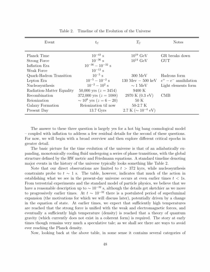
Table 2. Timeline of the Evolution of the Universe

Event tU TU Notes

Planck Time 10−43 s 1019 GeV GR breaks downStrong Force 10−36 s 1014 GeV GUTInflation Era 10−36 − 10−32 sWeak Force 10−12 sQuark-Hadron Transition 10−5 s 300 MeV Hadrons formLepton Era 10−5 − 10−2 s 130 Mev − 500 keV e+ − e− annihilationNucleosynthesis 10−2 − 102 s ∼ 1 MeV Light elements formRadiation-Matter Equality 50,000 yrs (z = 3454) 9400 KRecombination 372,000 yrs (z = 1088) 2970 K (0.3 eV) CMBReionization ∼ 108 yrs (z = 6− 20) 50 KGalaxy Formation Reionization til now 50-2.7 KPresent Day 13.7 Gyrs 2.7 K (∼ 10−4 eV)

The answer to these three question is largely yes for a hot big bang cosmological model– coupled with inflation to address a few residual details for the second of these questions.For now, we will begin with a broad overview and then explore different critical epochs ingreater detail.

The basic picture for the time evolution of the universe is that of an adiabatically ex-panding, monotonically cooling fluid undergoing a series of phase transitions, with the globalstructure defined by the RW metric and Friedmann equations. A standard timeline denotingmajor events in the history of the universe typically looks something like Table 2.

Note that our direct observations are limited to t > 372 kyrs, while nucleosynthesisconstraints probe to t ∼ 1 s. The table, however, indicates that much of the action inestablishing what we see in the present-day universe occurs at even earlier times t < 1s.From terrestrial experiments and the standard model of particle physics, we believe that wehave a reasonable description up to ∼ 10−32 s, although the details get sketchier as we moveto progressively earlier times. At t ∼ 10−32 there is a postulated period of superluminalexpansion (the motivations for which we will discuss later), potentially driven by a changein the equation of state. At earlier times, we expect that sufficiently high temperaturesare reached that the strong force is unified with the weak and electromagnetic forces, andeventually a sufficiently high temperature (density) is reached that a theory of quantumgravity (which currently does not exist in a coherent form) is required. The story at earlytimes though remains very much a speculative tale; as we shall see there are ways to avoidever reaching the Planck density.

Now, looking back at the above table, in some sense it contains several categories of

48

events. One category corresponds to the unification scales of the four fundamental forces.A second corresponds to the evolution of particle species with changing temperatures. Thistopic is commonly described as the thermal history of the universe. A third category describeskey events related to the Friedmann equations (radiation-matter equality, inflation). Finally,The last few events in this table correspond to the formation and evolution of the large scalestructures that we see in the universe today. Clearly each of these subjects can fill a semester(or more) by itself, and in truth all of these “categories” are quite interdependent. We willaim to focus on specific parts of the overall picture that illuminate the overall evolutionaryhistory. For now, let us begin at the “beginning”.

18 The Planck Time

Definition

The Planck time (∼ 10−43s) corresponds to the limit in which Einstein’s equations are nolonger valid and must be replaced with a more complete theory of quantum gravity if wewish to probe to earlier times. An often used summary of GR is that “space tells matterhow to move; matter tells space how to curve”. The Planck time and length essentiallycorrespond to the point at which the two cannot be considered as independent entities.

There are several ways to define the Planck time and Planck length. We will go throughtwo. The first method starts with the Heisenberg uncertainty principle, and defines thePlanck time as the point at which the uncertainty of the wavefunction is equal to the particlehorizon of the universe,

∆x∆p = lPmpc = h, (272)

where lP = ctP .Now, mP is the mass within the particle horizon, and

mP = ρP l3P . (273)

At early times we know that ρ ∼ ρc and tU ∼ 12H−1, so the density can be approximated as

ρP ∼ ρc =3H2

8πG∼ 1

Gt2P∼ c2

Gl2P, (274)

so

lP ≃(

Gh

c3

)1/2

≃ 2× 10−33cm, (275)

tP = lP/c ≃(

Gh

c5

)1/2

≃ 10−43s, (276)

ρP ≃1

Gt2P≃ 4× 1093gcm−3, (277)

49

mP ≃ ρl3P ≃(

hc

G

)1/2

≃ 3× 10−5g, (278)

EP = mP c2 ≃

(

hc5

G

)1/2

≃ 10−19GeV. (279)

Additionally, we can also define a Planck temperature,

TP ≃EPk≃ 1032K. (280)

Just for perspective, it is interesting to make a couple of comparisons. The Large HadronCollider (LHC), which will be the most advanced terrestrial accelerator when it becomesfully operational, is capable of reaching energies E ∼ 7 × 103 GeV, or roughly 10−15EP .Meanwhile, the density of a neutron star is ρN ∼ 1014 g cm−3, or roughly 10−79ρP .

The second way to think about the Planck length is in terms of the Compton wavelengthand the Schwarzschild radius. To see this, consider a particle of mass m. The Comptonlength of the particle’s wavefunction is

λC ≡h

∆p=

h

mc. (281)

The Compton wavelength in essence defines the scale over which the wavefunction is localized.Now consider the Schwarzschild radius of a body of mass m,

rs =2Gm

c2. (282)

By definition, any particle within the Schwarzschild radius lies beyond the event horizon andcan never escape.

The Planck length can be defined as the scale at which the above two equations are equal.Equating the two relations, we find that the Planck mass is

mP =

(

hc

2G

)1/2

≃(

hc

G

)1/2

, (283)

and that Planck length is

lP =2G

c2mp ≃

(

Gh

c3

)1/2

, (284)

from which the other definitions follow. Note that if the Schwarzschild radius is less than thewavefunction, then this would indicate that information (and mass) can escape from within.This would equivalent to having a naked singularity.

Physical Interpretation

50

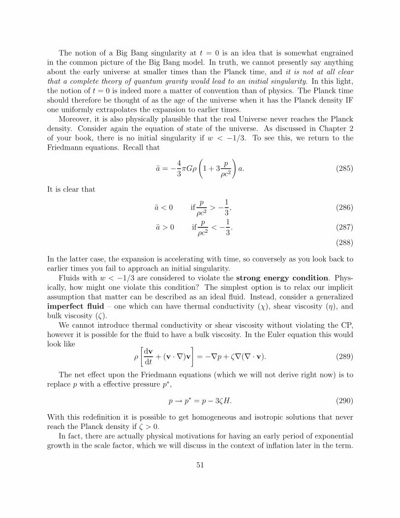
The notion of a Big Bang singularity at t = 0 is an idea that is somewhat engrainedin the common picture of the Big Bang model. In truth, we cannot presently say anythingabout the early universe at smaller times than the Planck time, and it is not at all clearthat a complete theory of quantum gravity would lead to an initial singularity. In this light,the notion of t = 0 is indeed more a matter of convention than of physics. The Planck timeshould therefore be thought of as the age of the universe when it has the Planck density IFone uniformly extrapolates the expansion to earlier times.

Moreover, it is also physically plausible that the real Universe never reaches the Planckdensity. Consider again the equation of state of the universe. As discussed in Chapter 2of your book, there is no initial singularity if w < −1/3. To see this, we return to theFriedmann equations. Recall that

a = −4

3πGρ

(

1 + 3p

ρc2

)

a. (285)

It is clear that

a < 0 ifp

ρc2> −1

3, (286)

a > 0 ifp

ρc2< −1

3. (287)

(288)

In the latter case, the expansion is accelerating with time, so conversely as you look back toearlier times you fail to approach an initial singularity.

Fluids with w < −1/3 are considered to violate the strong energy condition. Phys-ically, how might one violate this condition? The simplest option is to relax our implicitassumption that matter can be described as an ideal fluid. Instead, consider a generalizedimperfect fluid – one which can have thermal conductivity (χ), shear viscosity (η), andbulk viscosity (ζ).

We cannot introduce thermal conductivity or shear viscosity without violating the CP,however it is possible for the fluid to have a bulk viscosity. In the Euler equation this wouldlook like

ρ

[

dv

dt+ (v · ∇)v

]

= −∇p + ζ∇(∇ · v). (289)

The net effect upon the Friedmann equations (which we will not derive right now) is toreplace p with a effective pressure p∗,

p→ p∗ = p− 3ζH. (290)

With this redefinition it is possible to get homogeneous and isotropic solutions that neverreach the Planck density if ζ > 0.

In fact, there are actually physical motivations for having an early period of exponentialgrowth in the scale factor, which we will discuss in the context of inflation later in the term.

51

Given our lack of knowledge of the equation of state close to the Planck time, the abovescenario remains plausible. Having briefly looked at the earliest time, we now shift focus andwill spend a while talking about the evolution from the lepton era through recombination.

19 Temperature Evolution, Recombination and Decou-

pling

Before exploring the thermal history of the universe in the big bang model, we first need toknow how the temperature scales with redshift. This will give us our first glimpse of the cos-mic microwave background. Below we are concerned with matter and radiation temperatureswhen the two are thermally decoupled and evolving independently.

19.1 The Adiabatic and LTE Assumptions

Throughout this course we have been making the assumption that the matter and radiationdistributions are well-approximated as an adiabatically expanding ideal fluid. For much ofthe early history of the universe, we will also be assuming that this fluid is approximately inlocal thermodynamic equilibrium (LTE). It is worth digressing for a few moments to discusswhy these are both reasonable assumptions.

Adiabatic ExpansionIn classical thermodynamics, an expansion is considered to be adiabatic if it is “fast” in

the sense that the gas is unable to transfer heat to/from an external reservoir on a timescaleless than the expansion. The converse would be an isothermal expansion, in which thepressure/volume are changed sufficiently slowly that the gas can transfer heat to/from anexternal reservoir and maintain a constant temperature. Mathematically, the above conditionfor adiabatic expansion corresponds to PV =constant and dE = −PdV .

In the case of the universe, the assumption of adiabatic expansion is a basic consequence ofheat. Having a non-adiabatic expansion would require a means of transferring heat betweenour universe and some external system (an adjacent brane?). Moreover, this heat transferwould need to occur on a timescale t << tH for the adiabatic assumption to fail. One canalways postulate scenarios in which there is such a transfer (e.g. the steady-state model);however, there is no physical motivation for doing so at present. Indeed, the success of BigBang nucleosynthesis can be considered a good argument back to t ∼ 1s for the sufficiencyof the adiabatic assumption.

Local Thermodynamic Equilibrium (LTE)The condition of LTE implies that the processes acting to thermalize the fluid must occur

rapidly enough to maintain equilibrium. In an expanding universe, this is roughly equivalentto saying that the collision timescale is less than a Hubble time, τ ≤ tH . Equivalently, onecan also say that the interaction rate, Γ ≡ nσ|v| ≥ H . Here n is the number density ofparticles, σ is the interaction cross-section, and |v| is the amplitude of the velocity.

52

Physically, the above comes from noting that T ∝ a−1 (which we will derive shortly)and hence T /T = −H , which says that the rate of change in the temperature is just setby the expansion rate. Once the interaction rate drops below H , the average particle has amean free path larger that the Hubble distance, and hence that species of particle evolvesindependently from the radiation field henceforth. It is worth noting that one cannot assumea departure from thermal equilibrium just because a species is no longer interacting – it ispossible for the temperature evolution to be the same as that of the radiation field if noadditional processes are acting on either the species or the radiation field.

19.2 Non-relativistic matter

In this section we will look at the temperature evolution of non-relativistic matter in thecase where the matter is decoupled from the radiation field. If we assume that the mattercan be described as an adiabatically expanding ideal gas, then we know

dE = −PdV ; (291)

E = U +KE =(

ρmc2 +

3

2nkBTm

)

V =

(

ρmc2 +

3

2

ρmkBTmmp

)

a3; (292)

P = nkBTm =ρmkBTmmp

, (293)

and putting these equations together can quickly see

d

[(

ρmc2 +

3

2ρm

kBTmmp

)

a3

]

= −ρmkBTmmp

da3. (294)

Mass conservation requires also that ρma3 is constant, so

3

2

ρmkBa3dTm

mp= −ρmkBTM

mpda3, (295)

dTmTm

=2

3

da3

a3, (296)

Tm = T0m

(

a0

a

)2

= T0m(1 + z)2. (297)

So we see that the temperature of the matter distribution goes at (1 + z)2.

19.3 Radiation and Relativistic Matter

What about for radiation. For a gas of photons, it is straightforward to derive the redshiftdependence. The relation between the energy density and temperature for a black body issimply

< u >≡ ρrc2 = σrT

4r , (298)

53

and the pressure is

p =1

3ρc2 =

σrT4

3. (299)

Note that you may have seen this before in the context of the luminosity of a star withtemperature T . The quantity σr is the radiation density constant, which in most placesyou’ll see written at a instead. The value of the radiation constant is

σr =π2k4

B

15h3c3= 7.6× 10−15ergscm−3K4. (300)

We know from a previous class that

ρr ∝ (1 + z)4, (301)

which tells us thatTr = T0r(1 + z). (302)

This is true for any relativistic species, and more generally the temperature of any particlespecies that is coupled to the radiation field will have this dependence.

One could also derive the same expression using the adiabatic expression

d(σrT4a3) = −σrT

4

3da3. (303)

4T 3dTa3 + T 4da3 = −T4

3da3 (304)

dT

T= −1

3

da3

a3(305)

T ∝ a−1 ∝ (1 + z). (306)

19.4 Temperature Evolution Prior to Decoupling

In the above two sections we have looked at the temperature evolution of non-relativisticmatter and radiation when they are evolving as independent, decoupled systems:

Tm = T0m(1 + z)2 (307)

Tr = T0r(1 + z)1 (308)

(309)

What about before decoupling? In this case, the adiabatic assumption becomes

d

[(

ρmc2 +

3

2ρm

kBTmmp

+ σrT4

)

a3

]

= −(

ρmkBTmmp

+σrT

4

3

)

da3. (310)

Mass conservation (valid after freeze-out) requires that ρma3=constant, as before. We are

now going to introduce a dimensionless quantity σrad, which will be important in subsequentdiscussions. We define

σrad = σr4mpT

3

3kBρm. (311)

54

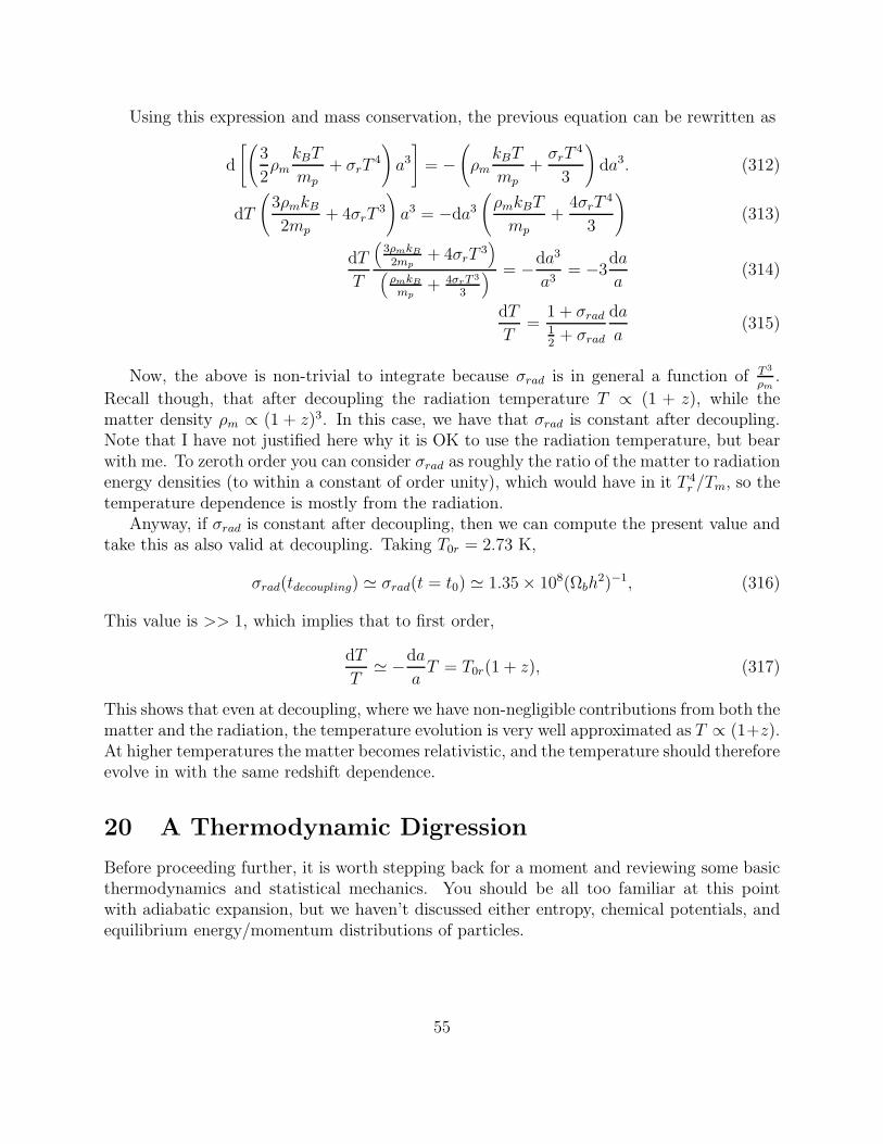
Using this expression and mass conservation, the previous equation can be rewritten as

d

[(

3

2ρm

kBT

mp+ σrT

4

)

a3

]

= −(

ρmkBT

mp+σrT

4

3

)

da3. (312)

dT

(

3ρmkB2mp

+ 4σrT3

)

a3 = −da3

(

ρmkBT

mp+

4σrT4

3

)

(313)

dT

T

(

3ρmkB

2mp+ 4σrT

3)

(

ρmkB

mp+ 4σrT 3

3

) = −da3

a3= −3

da

a(314)

dT

T=

1 + σrad12

+ σrad

da

a(315)

Now, the above is non-trivial to integrate because σrad is in general a function of T 3

ρm.

Recall though, that after decoupling the radiation temperature T ∝ (1 + z), while thematter density ρm ∝ (1 + z)3. In this case, we have that σrad is constant after decoupling.Note that I have not justified here why it is OK to use the radiation temperature, but bearwith me. To zeroth order you can consider σrad as roughly the ratio of the matter to radiationenergy densities (to within a constant of order unity), which would have in it T 4

r /Tm, so thetemperature dependence is mostly from the radiation.

Anyway, if σrad is constant after decoupling, then we can compute the present value andtake this as also valid at decoupling. Taking T0r = 2.73 K,

σrad(tdecoupling) ≃ σrad(t = t0) ≃ 1.35× 108(Ωbh2)−1, (316)

This value is >> 1, which implies that to first order,

dT

T≃ −da

aT = T0r(1 + z), (317)

This shows that even at decoupling, where we have non-negligible contributions from both thematter and the radiation, the temperature evolution is very well approximated as T ∝ (1+z).At higher temperatures the matter becomes relativistic, and the temperature should thereforeevolve in with the same redshift dependence.

20 A Thermodynamic Digression

Before proceeding further, it is worth stepping back for a moment and reviewing some basicthermodynamics and statistical mechanics. You should be all too familiar at this pointwith adiabatic expansion, but we haven’t discussed either entropy, chemical potentials, andequilibrium energy/momentum distributions of particles.

55

20.1 Entropy

Entropy is a fundamental quantity in thermodynamics that essentially describes the disorderof a system. The classical thermodynamic definition of entropy is given by

dS =dQ

T, (318)

where S is the entropy and Q is the heat of the system. In a more relevant astrophysicalcontext, the radiation energy density for instance would be

sr =< u >

T=ρc2 + p

T. (319)

The statistical mechanics definition is based instead upon the number of internal “micro-states” in a system (essentially internal degrees of freedom) for a given macro-state. Asan example, consider the case of 10 coins. There is one macro-state corresponding to allheads, and also only 1 micro-state (configuration of the individual coins) that yields thismacro-state. On the other hand, for the macro-state with 5 heads and 5 tails, there areC(10,5) combinations of individual coins - micro-states - that can yield a single macro-state.By this Boltzmann definition, the entropy is S = kB lnω, where ω is the number of internalmicro-states.

21 Chemical Potential

I’ve never liked the name chemical potential, as the ‘chemical’ part is mainly a historicalartifact. What we’re really referring here to is the potential for electromagnetic and weak(and strong at high T) reactions between particles. In this particular instance, I’ll quote thedefinition of chemical potential from Kittel & Kroemer (page 118). Consider two systemsthat can exchange particles and energy. The two systems are in equilibrium with respect toparticle exchange when the net particle flow is zero. In this case:

“The chemical potential governs the flow of particles between the systems, just as thetemperature govers the flow of energy. If two systems with a single chemical species are atthe same temperature and have the same value of the chemical potential, there will be nonet particle flow and no net energy flow between them. If the chemical potentials of the twosystems are different, particles will flow from the system at higher chemical potential to thesystem at lower chemical potential.”

In the cosmological context that we are considering, instead of looking at physicallymoving particles between two systems, what we are instead talking about is convertingone species of particle to another. In this interpretation, what the above statement saysis that species of particles are in equilibrium (chemical equilibrium, but again I loathe theterminology), then the chemical potential of a given species is related to the potentials ofthe other species with which it interacts. For instance, consider four species a, b, c, d thatinteract as

a+ b←→ c + d. (320)

56

For this reaction, µa + µb = µc + µd whenever chemical equilibrium holds.For photons, µγ = 0, and indeed in for all species in the early universe it is reasonable

to approximate µi = 0 (i.e. µi << kT ). This can be seen for example by considering thereaction

γ + γ e+ + e−. (321)

If this reaction is in thermal equilibrium (i.e. prior to pair annihilation), then the chemicalpotential must be

µ+ + µ− = 0. (322)

In addition, sincene− = ne++ ∼ 10−9, (323)

we expectµ+ = µ−+ ∼ 10−9. (324)

Hence,µ+ ≃ µ− ≃ 0. (325)

21.1 Distribution Functions

Long ago, in a statistical mechanics class far, far away, I imagine that most of you discusseddistribution functions for particles. For species of indistinguishable particles in kineticequilibrium the distribution of filled occupation states is given either by the Fermi-Diracdistribution (for fermions) or the Bose-Einstein distribution (for bosons), which are given by

f(p) =1

e(E−µ)/kT ± 1, (326)

where p in this equation is the particle momentum and E2 = |p|2c2 + (mc2)2). The “+”corresponds to Fermions and the “-” corresponds to bosons.

Physically the reason that the equation is different for the two types of particles is due totheir intrinsic properties. Fermions, which have half integer spin, obey the Pauli exclusionprinciple, which means that no two identical fermions can occupy the same quantum state.Bosons, on the other hand, do not obey the Pauli exclusion principle and hence multiplebosons can occupy the same quantum state. This is a bit of a digression at this point, so Irefer the reader to Kittel & Kroemer for a more detailed explanation.

Note that the above distribution functions hold for indistinguishable particles. By defini-tion, particles are indistinguishable if their wavefunctions overlap. Conversely, are considereddistinguishable if their physical separation is large compared to their De Broglie wavelength.In the classical limit of distinguishable particles, the appropriate distribution function is theBoltzmann distribution function,

f(p) =1

e(E−µ)/kT, (327)

57

which can be seen to be the limiting case of the other distributions when kT << E (i.e. thenon-relativistic limit).

Getting back to the current discussion, for any given species of particles that we will bediscussing in the context of the early universe, the total number density of particles is foundby integrating over the distribution function,

n =g

h3

∫

f(p)d3p. (328)

In the above equation, the quantity g/h is the density of states available for occupation(can be derived from a particle-in-a-box quantum mechanical argument). The quantity gspecifically refers to the number of internal degrees of freedom. We will return to this in amoment.

Similar to the number density, the energy density can be written as written as

< u >= ρc2 =g

h3

∫

E(p)f(p)d3p. (329)

From the distribution functions and definition of energy, these equations can be rewrittenas

n =g

2π2h3c3

∫ ∞

m

(E2 − (mc2)2)1/2EdE

exp[(E − µ)/kT ]± 1(330)

ρ =g

2π2h3c3

∫ ∞

m

(E2 − (mc2)2)1/2E2dE

exp[(E − µ)/kT ]± 1. (331)

In the relativistic limit, the above equations become

n =g

2π2h3c3

∫ ∞

0

E2dE

exp[(E − µ)/kT ]± 1(332)

ρ =g

2π2h3c3

∫ ∞

0

E3dE

exp[(E − µ)/kT ]± 1. (333)

Note that Kolb & Turner §3.3-3.4 is a good reference for this material.Now, let us consider a specific example. Photons obey Bose-Einstein statistics, so the

number density is

nγ =g

2π2h3c3

∫ ∞

0

E2dE

exp[(E − µ)/kT ]± 1. (334)

As we will discuss later, for photons the chemical potential is µγ = 0, so making the substi-tution x = E/kT the above equation becomes

g

2π2

(

kT

hc

)3∫ ∞

0

x2dx

ex − 1. (335)

It turns out that this integral corresponds to the Riemann-Zeta function, which is definedsuch that

ζ(n)Γ(n) =∫ ∞

0

xn−1dx

ex − 1, (336)

58

for integer values of n. Also, for photons g = 2 (again, we’ll discuss this in a moment). Theequation for the number density of photons thus becomes,

nγ =1

π2

(

kT

hc

)3

ζ(3)Γ(3) =2ζ(3)

π2

(

kT

hc

)3

. (337)

For the current Tr = 2.73 K, and given that ζ(3) ≃ 1.202, we have that n0γ = 420 cm−3.Note that since nγ scales with T 3, nγ ∝ (1 + z)3 for redshift intervals where no species arefreezing out.

More generally, we have noted above that the chemical potential for all particle speciesin the early universe is zero. Consequently, in a more general derivation it can be shownthat for any relativistic particle species

ni = gi

(

kT

hc

)3∫ ∞

0

x2dx

ex ± 1= α

giζ(3)

π2

(

kBT

hc

)3

, (338)

where α = 3/4 for fermions and α = 1 for bosons. Similarly, the energy density of a givenspecies is given by

ρi = gi(kT )4

(hc)3

∫ ∞

0

x3dx

ex ± 1= β

gi2σrT

4. (339)

where β = 7/8 for fermions and β = 1 for bosons.For a multi-species fluid, the total energy density will therefore be

ρc2 =

∑

bosons

gi +7

8

∑

fermions

gi

σrT4

2= g∗

σrT4

2. (340)

21.2 What is g?

A missing link at this point is this mysterious g, which I said is the number of internaldegrees of freedom. In practice, what this means for both bosons and fermions is that

g = 2× spin + 1. (341)

For example, for a spin 1/2 electron or muon, g = 2. Two exceptions to this rule are photons(g = 2) and neutrinos (g = 1), which each have one less degree of freedom than you mightexpect from the above relation. The underlying reasons are unimportant for the currentdiscussion, but basically the photon is down by one because longitudinal E&M waves don’tpropagate, and neutrinos are down one because one helicity state does not exist.

In the above section we showed how to combine the g of the different particle species toobtain an effective factor g∗ for computing the energy density for a multispecies fluid. Justto give one concrete (but not physical) example, consider having a fluid comprised of onlyνe and µ+. In this case,

g∗ = 0 +7

8(1 + 2) =

21

8(342)

59

22 Photon-Baryon Ratio

OK – time to return to cosmology from thermodynamics, although at this point we’re stilllaying a bit of groundwork. One important quantity is the ratio between the present meannumber density of baryons (n0b) and photons (n0γ). It’s actually defined in the book con-versely as η0 = n0b/n0γ . The present density of baryons is

n0b =ρ0b

mp≃ 1.12× 10−5Ω0bh

2cm−3. (343)

Meanwhile, we have now calculated the photon density in a previous section,

n0γ =2ζ(3)

π2

(

kBT0r

hc

)3

≃ 420cm−3 (344)

The photon-baryon ratio therefore is

η−10 =

n0b

n0γ

≃ 3.75× 107(Ω0bh2)−1. (345)

The importance of this quantity should become clearer, but for now the key thing to note isthat there are far more photons than baryons.

23 Radiation Entropy per Baryon

Related to the above ratio, we can also ask what is ratio between the radiation entropydensity and the baryon density? From our definition of entropy earlier, we have

sr =< u >

T=ρrc

2 + p + r

T=

4

3

ρrc2

T=

4

3σrT

3. (346)

We also know that the number density of baryons is

nb = ρbmp (347)

Recalling that σrad = 4mpσrT30r/(3kbρ0b), we can rewrite the equation for the entropy as

sr = σradkbnb, (348)

orσrad =

srkBnb

=srnγkBη

, (349)

which tells us that σrad, sr, and η−1 are all proportional. Your book actually takes the aboveequation and fills in numbers to get σrad = 3.6η−1 to show that the constant is of order unity.

Finally, and perhaps more interestingly, σrad is also related to the primordial baryon-antibaryon asymmetry. Subsequent to the initial establishment of the asymmmetry, (nb −

60

nb)a3 must be a conserved quantity (conservation of baryon number). Moreover, in the

observed universe nb → 0, so n0ba3 is conserved. At early times when the baryon species are

in equilibrium, we havenb ≃ nb ≃ nγ ∝ T 3 ∝ (1 + z)3. (350)

At this stage the baryon asymmetry is expected to be

nb − nbnb + nb

≃ nb − nb2nγ

≃ n0b

2n0γ≃ 1.8σ−1

rad. (351)

From a physical perspective, what this says is that the reason that σrad is so large, andthat there are so many more photons than baryons, is that the baryon-antibaryon asymmetryis small.

24 Lepton Era

The Lepton era corresponds the time period when the universe is dominated by leptons,which as you will recall are particles that do not interact via the strong force. The threefamilies of leptons are the electron (e±, νe, νe), muon (µ±, νµ, νµ), and tau (τ±, ντ , ντ ) families.

The lepton era begins when pions (a type of hadron with a short lifetime) freeze-out atT ∼ 130 MeV, annihilating and/or decaying into photons. At the start of the lepton era,the only species that are in equilibrium are the γ,e±,µ±, a small number of baryons, andneutrinos (all 3 types).

It is of interest to calculate g∗ at both the beginning and end of the lepton era (both forpractice and physical insight). At the start of the lepton era (right after pion annihilation),

g∗start = 2 +7

8× (2× 2 + 2× 2 + 3× 2) = 14.25 (352)

where the terms correspond to the photons, electrons, muons, and neutrinos, respectively.[We’llignore the baryons.] At the end of the lepton era, right after the electrons annihilate, we areleft with only the photons, so

g∗end = 2. (353)

We’ll work out an example with neutrinos in a moment to show why this matters. The quickphysical answer though is that when species annihilate g decreases and the radiation energydensity increases (since particles are being converted into radiation). The value of g is usedto quantify this jump in energy density and temperature.

To see this, consider that in this entire analysis we are treating the universe as an adia-batically expanding fluid. We discussed previously that this is equivalent to requiring thatthere is no heat transfer to an external system, or

dS ≡ dQ

dT= 0. (354)

61

In other words, entropy is conserved as the universe expands. We also discussed previouslythat the entropy density is given by

sr =ρc2 + p

T, (355)

which in well-approximated by the radiative components, giving

sr =4

3

ρc2

T=

2

3g∗σrT

3. (356)

Now consider pair annihilation of a particle species at temperature T . From conservationof entropy, we require

sbefore = safter, (357)

2

3g∗beforeσrT

3before =

2

3g∗afterσrT

3after , (358)

g∗beforeT3before = g∗afterT

3after , (359)

(360)

or

Tafter = Tbefore

(

g∗beforeg∗after

)1/3

(361)

Now, g∗ is a decreasing function as particles leave equilibrium, so the above equation statesthat the radiation temperature is always higher after annihilation of a species.

There are two relevant types of interactions during the lepton era that act to keep particlesin equilibrium – electromagnetic and weak interactions. Examples of the electromagneticinteractions are

p + p n + n π+ + π− µ+ + µ− e+ + e− π0 2γ, (362)

and examples of weak interactions are

e− + µ+ νe + νµ, (363)

e− + e+ νe + νe, (364)

e− + p νe + n, (365)

e− + νe e+ + νe. (366)

(367)

The relevant cross-sections for electromagnetic interactions is the Thomson cross-section(σT ), while the weak interaction cross-section σwk ∝ T 2 is given in your book.

Note that neutrinos feel the weak force, but not the electromagnetic force. This property,coupled with the temperature dependence of the weak interaction cross-section, is the reasonthat neutrinos are so difficult to detect.

62

24.1 Electrons

The electron-positron pairs remain in equilibrium during the entire lepton era since thecreation timescale for pairs is much less than the expansion timescale. Indeed the electronsremain in equilibrium until recombination, which we will discuss shortly. In practice, theend of the lepton era is defined by the annihilation of the electrons and positrons at T ∼ 0.5MeV.

What is the density of electron-positron pairs? For T > 1010K, electromagnetic‘ interac-tions such as γ + γ e+ + e− are in thermal equilibrium. Using the fermion phase spacedistributions, we have

ne± = ne− + ne+ =3

4

ζ(3)

π2(2× ge)

(

kBTehc

)3

=3ζ(3)

π2

(

kBTehc

)3

, (368)

ρe±c2 = ρe+c

2 + ρe−c2 =

7

8(2 + 2)

σrT4e

2=

7

4σrT

4e . (369)

Since the electrons are in equilibrium, Te = Tr.

24.2 Muons

The muon pairs also remain in equilibrium until T ∼ 1012K, at which point they annihilate.It is straightforward to work out that before annihilation the muons should have the samenumber and energy densities as the electrons.

24.3 Neutrinos

Electron neutrinos decouple from the rest of the universe when the timescale for weak inter-action processes such as νe + νe e+ + e− equals the expansion timescale. Other neutrinospecies are coupled to the νe via neutral current interactions, so they decouple no later thanthis. To be specific, the condition for neutrino decoupling is

tH ≃ 2

(

3

32πGρ

)1/2

< tcollision ≃ (nlσwkc)−1, (370)

where nl is the number density of a generic lepton. At this time period τ particles are nolonger expected to be in equilibrium, and we have noted above that ne = nµ, so the relevantdensity is given by the above equation for ne± as nl = (1/2)ne±. Similarly,

ρl = ρe±c2/2 =

7

8σrT

4. (371)

The condition for equilibrium, with insertion of constants, becomes

tHtcoll≃(

T

3× 1010K

)3

< 1 (372)

63

24.3.1 Temperature of Relic Species: Neutrinos as an Example

It is interesting to consider the neutrino temperature in order to illustrate the general char-acteristics of temperature evolution. Given that we know the current temperature of theradiation field, we can derive the neutrino temperature by expressing it in terms of theradiation temperature.

Neutrinos decouple from the radiation field at a time when they remain a relativisticspecies. Consequently, we expect their subsequent time evolution to follow the relation

T0ν = Tν,decoupling(1 + z)−1 (373)

We know that at decoupling Tν = Tr. If no particle species annihilate after the neutrinosdecouple, the Tr = T0r(1 + z) and we have T0ν = T0r. However, we know that neutrinosdecouple before electron-positron annihilation. We must therefore calculate how much thetemperature increased due to this annihilation We saw before that when a particle speciesannihilates

Tafter = Tbefore

(

g∗beforeg∗after

)1/3

, (374)

so what we need to do is calculate the g∗ before and after annihilation. Before annihilation,the equilibrium particle species are e± and photons, so

g∗ = 2 +7

8(2× 2) = 2 + 7/2 = 11/2. (375)

After annihilation, only the photons remain in equilibrium, so g∗ = 2. Consequently,

Tafter = Tbefore

(

11

4

)1/3

. (376)

which says that at the neutrino decoupling

Tr,decoupling = T0r

(

4

11

)1/3

(1 + z) (377)

and hence

T0ν = Tν,decoupling(1 + z)−1 =(

4

11

)1/3

T0r ≃ 1.9K. (378)

24.3.2 Densities of Relic Species: Neutrinos as an Example

Once the neutrino temperature is known, the number density can be calculated in the stan-dard fashion:

nν =3

4

ζ(3)

π2(3× 2× 1)

(

kBTνhc

)3

≃ 324cm−3. (379)

64

where we have assumed 3 neutrino species. If neutrinos are massless, we can also computethe energy density as

ρνc2 =

7

8(3× 2× 1)

σrT4ν

2=

7

4σrT

4e ≃ 3× 10−34g cm−3. (380)

In the last few years, terrestrial experiments have however demonstrated that there mustbe at least one massive neutrino species (a consequence of neutrinos changing flavor, whichcannot happen if they are all massless). The number density calculation above is unaffectedif neutrinos are massive, but looking at the number one sees that this is roughly the same asthe photon number density (or of order 109 times the baryon number density). Consequently,even if neutrinos were to have a very small rest mass, it is possible for them to contributea non-negligible amount to the total energy density. To be specific, the mass density ofneutrinos is

ρ0ν =< mν > n0ν ≃ Nν × 1.92× < mν >

10eV× 10−30g cm−3, (381)

or in terms of critical density,

Ω0ν ≃ 0.1×Nν< mν >

10eV× h−2. (382)

Astrophysical constraints based upon the CMB and large scale structure indicate that thecombined mass of all neutrino species is

∑

mν ≤ 1eV (383)

(assuming General Relativity is correct), or < mν >≤ 1/3 eV for Nν = 3, which implies that

Ω0ν ≤ 0.005. (384)

One can ask whether the relic neutrinos remain relativistic at the current time. Roughlyspeaking, the neutrinos will cease to be relativistic when

ρkineticρrestmass

≤ 1. (385)

We calculated that at the current time, for a given type of neutrino, the kinetic energydensity is

ρkinetic = 10−34g cm−3. (386)

and the rest energy is

ρ0ν =≃ 1.92× < mν >

10eV× 10−30g cm−3, (387)

so we see that the neutrinos are no longer relativistic if

µν ≥10−34

1.92× 10−30× 10 eV, (388)

µν ≥ 5× 10−4 eV. (389)

65

We know that at least one of the species of neutrinos is massive (see section 8.5 of yourbook for more details), but given this limit cannot say whether some of the neutrino speciesare non-relativistic at this time.

Finally, it is worth reiterating that we found that the neutrinos, which were relativisticat decoupling, have a temperature dependence after decoupling of Tν ∝ (1 + z). This willremain true even after the neutrinos become non-relativistic. Recall that the temperatureis defined in terms of the distribution function – this distribution remains valid when theparticles become non-relativistic. On the other hand, a species that is non-relativistic whenit decouples has T ∝ (1 + z)2. Thus, the redshift dependence of the temperature fora given particle subsequent to decoupling is determined simply by whether theparticle is relativistic at decoupling.

24.4 Neutrino Oscillations

This is an aside for interested readers.Why do we believe that at least one species of neutrinos has a non-zero mass? The

basic evidence comes from observations of solar neutrinos and the story of the search forneutrino mass starts with the “solar neutrino problem”. In the standard model of stellarnucleosynthesis, the p− p chain produces neutrinos via reactions such as

p+ p→ D + e+ + νe;Eν = 0.26MeV (390)

Be7 + e− → Li7 + νe;Eν = 0.80MeV (391)

B8 → Be7 + e+ + νe;Eν = 7.2MeV. (392)

The physics is well-understood, so if we understand stellar structure then we can make aprecise prediction for the solar neutrino flux at the earth. In practice, terrestrial experimentsto detect solar neutrinos find a factor of a few less νe than are expected based upon thestandard solar model.

Initially, there were two proposed solutions to the solar neutrino problem. One proposedresolution was that perhaps the central temperature of the sun was slightly lower, whichwould decrease the expected neutrino flux. Helioseismology has now yielded sound speedsover the entire volume of the sun to 0.1% and the resulting constraints on the central tem-perature eliminate this possibility. The second possible solution is “neutrino oscillations”.The idea with neutrino oscillations is that neutrinos can self-interact and transform to dif-ferent flavors. Since terrestrial experiments are only capable of detecting νe, we should onlyobserve 1/3 to 1/2 of the expected flux if the electron neutrinos produces in the sun convertto other types.

Now, what does this all have to do with neutrino mass? The answer comes from thephysics behind how one can get neutrinos to change flavors. The basic idea is to postulatethat perhaps the observed neutrino types are not fundamental in themselves, but insteadcorrespond to linear combinations of neutrino eigenstates. As an example, consider oscil-lations between only electron and muon neutrinos and two eigenstates ν1 and ν2. Given a

66

mixing angle θ, one could construct νe and νµ states as

νe = cos θν1 + sinθν2, (393)

νµ = sin θν1 − sin θν2. (394)

(imaging the above in bra-ket notation...not sure how to do this properly in latex)Essentially, the particle precesses between the νe and νµ states. If the energies corre-

sponding to the eigenstates are E1 and E2, then the state will evolve as

νe = cos θ exp(−iE1t/h)ν1 + sin θ exp(−iE2t/h)ν2, (395)

and the probability of finding a pure electron state will be

Pνe(t) = |νe(t)|2 = 1− sin2(2θ) sin2

[

1

2(E1 −E2)t/h

]

. (396)

If both states have the same momenta (and how could they have different momenta?),then the energy difference is simple

∆E =∆m2c4

E1 + E2. (397)

The important thing to notice in the above equation is that the oscillations do not occurif the two neutrinos have equal mass. There must therefore be at least one flavor of neutrinothat has a non-zero mass.

25 Matter versus Radiation Dominated Eras

One key benchmark during this period is the transition from a radiation to matter-dominateduniverse. We have seen in earlier sections that the redshift evolution of the energy densityfor non-relativistic matter is different than for relativistic particles and photons. Specifically,ρ = ρ0(1 + z)3(w+1), where w ≈ 0 for non-relativistic matter and w = 1/3 for relativisticparticles and photons. While non-relativistic matter is the dominant component at z = 0,the practical consequence of this density definition is that

ρrρm

=ρ0r

ρ0m(1 + z), (398)

which means that above some redshift the energy density of relativistic particles dominatesand the radiative term in the Friedmann equations becomes critical. The current radiationenergy density is

ρr =g

2

σrT4

c2=σrT

4

c2= 4.67× 10−34g cm−3, (399)

while the current matter density is

ρ0m = ρocΩ0mh2 = (1.9× 10−29)0.27h2g cm−3 ≃ 2.5× 10−30h2

70g cm−3. (400)

67

Considering just these two components, we would expect the matter and radiation den-sities to be equal at

1 + zeq =ρ0m

ρ0r∼ 5353. (401)

In practice, the more relevant timescale is the point when the energy density of non-relativistic matter (w = 0) is equal to the energy density in all relativistic species (w = 1/3).To correctly calculate this timescale, we also need to fold in the contribution of neutrinos.Using the relations that we saw earlier, the energy density of the photons + neutrinos shouldbe

ρrel = ρr + ρν =(

σrT4r +

7

8Nν

gν2σrT

4ν

)

c−2. (402)

In our discussion of the lepton era and evolution of the neutrinos we worked out (or willwork out) that Tν = (4/11)1/3Tr. We also know that gν = 1, and the best current evidenceis that there are 3 neutrino species (Nν = 3) plus their antiparticles (so 3× 2), which meansthat the above equation can be written as

ρrel =σrT

4r

c2

[

1 + (2×Nν)7

812(

4

11

)4/3]

= 1.68σrT4 = 1.681ρr. (403)

In your book, the coefficient (1.68) used to include the total relativistic contribution fromphotons and neutrinos is denoted at K0, and at higher densities the factor is called Kc toaccount for contributions from other relativistic species. In practice, Kc ∼ K0, so we’ll stickwith K0.

If we now use this energy density in calculating the epoch of matter-radiation equality,we find that

1 + zeq =ρ0m

ρ0rel∼ 5353/1.68 ≃ 3190. (404)

The most precise current determination from WMAP gives zeq = 3454 (tu ∼ 50 kyrs).This is the redshift at which the universe transitions from being dominated by radiationand relativistic particles to being dominated by non-relativistic matter. At earlier times theuniverse is well-approximated by a simple radiation-dominated EdS model. During this era,

E(z) ≃ (1 + z)√

K0Ω0r (405)

It is worth noting that the most distant direct observations that we currently have comefrom the cosmic microwave background at z = 1088, so all existing observations are in thematter dominated era.

26 Big Bang Nucleosynthesis

Cosmological nucleosynthesis occurs just after electron-positron pairs have annihilated atthe end of the lepton era. From an anthropic perspective this is perhaps one of the most

68

important events in the history of the early universe – by the end of BBN at t ≃ 3 minutesthe primordial elemental abundances are fixed.

Let us begin with the basic conceptual framework and definitions. There are basicallytwo ways to synthesize elements heavier that hydrogen. The first method is the familiarprocess of stellar nucleosynthesis, as worked out by Burbidge, Burbidge, Fowler, and Hoyle.This method is good for producing heavy elements (C,N,O, etc), but cannot explain theobserved high fraction of helium in the universe,

Y ≡ mHe

mtot≃ 0.25. (406)

The second method is cosmological nucleosynthesis. The idea of elemental synthesis in theearly universe was put forward in the 1940’s by Gamov, Alpher, and Hermann, with thebasic idea being that at early times the temperature should be high enough to drive nuclearfusion. These authors found that, unlike stellar nucleosynthesis, cosmological (or Big Bang)nucleosynthesis could produce a high helium fraction. As we shall see though, BBN doesnot produce significant quantities of heavier elements. The current standard picture is thatBBN establishes the primordial abundances of the light elements, while the enrichment ofheavier elements is subsequently driven by stellar nucleosynthesis.

With that introduction, let’s dive in. Your book listed the basic underlying assumptionsthat are implicit to this discussion. Some of these are aspects of the Cosmological Principle(and apply to our discussion of other, earlier epochs as well); some are subtle issues that aresomewhat beyond the scope of our discussion. I reproduce the full list here for completeness:

1. The Universe has passed through a hot phase with T ≥ 1012 K, during which itscomponents were in thermal equilibrium.

2. The known laws of physics apply at this time.

3. The Universe is homogeneous and isotropic at this time.

4. The number of neutrino times is not high (Nν ≃ 3).

5. The neutrinos have a negligible degeneracy parameter.

6. The Universe does not contain some regions of matter and others of antimatter (sub-point of 2., and part of the CP).

7. There is no appreciable magnetic field at this epoch.

8. The photon density is greater than that of any exotic particles at this time.

69

26.1 Neutron-Proton Ratio

As a starting point, we need to know the relative abundances of neutrons and protons atthe start of nucleosynthesis. In kinetic equilibrium, the number density of a non-relativisticparticle species obeys the Boltzmann distribution, so

ni = gi

(

mikBT

2πh2

)3/2

exp

(

µi −mic2

kBT

)

. (407)

Neutrons and protons both have g = 2, and the µi can be ignored, which means that theratio of the two number densities is

nnnp≃(

mn

mp

)3/2

exp

(

−(mn −mp)c2

kBT

)

≃ e−Q/kBT , (408)

where Q = (mn −mp)c2 ≃ 1.3 MeV. Equivalently, this expression says that while the two

species are in thermal equilibrium,

nnnp≃ exp

(

−1.5× 1010K

T

)

. (409)

Equilibrium between protons and neutrons is maintained by weak interactions such asn + νe p + e−, which remain efficient until the neutrinos decouple. The ratio is thereforeset by the temperature at which the neutrinos decouple. Neutrinos decouple at T ≃ 1010K,in which case

Xn ≡n

n + p≃ 1

1 + exp(1.5)= 0.18. (410)

After this point, free neutrons can still transform to protons via β−decay, which has ahalf-life of τn = 900s. This, the subsequent relative abundances of free protons and neutronsis given by

Xn(t) ≡ Xn(teq)e−(t−teq)/τn . (411)

In practice, as we shall see nucleosynthesis lasts for << 900s, so Xn ≃ Xn(teq) for the entiretime period of interest.

26.2 Nuclear Reactions

Before proceeding, let us define the nuclear reactions that we may expect to occur. Theseinclude:

p+ n d(i.e.H2) + γ (412)

(413)

d+ n H3 + γ (414)

d+ d H3 + p (415)

70

d+ p He3 + γ (416)

d+ d He3 + n (417)

(418)

H3 + d He4 + n (419)

He3 + n He4 + γ (420)

He3 + d He4 + p. (421)

(422)

The net effect of all after the first of these equations is essentially

d+ d He4 + γ. (423)

What about nuclei with higher atomic weights? The problem is that there are no stablenuclei with atomic weights of either 5 or 8, which means that you can only produce heavierelements by “triple-reactions”, such as 3He4 → C12 + γ, in which a third nuclei hits theunstable nuclei before it has time to decay. The density during cosmological nucleosynthesisis far lower than the density in stellar interiors, and the total time for reactions is only ∼3minutes rather than billions of years. Consequently this process is far less efficient duringcosmological nucleosynthesis that stellar nucleosynthesis.

26.3 Deuterium

Let us now consider the expected abundance of helium produced. From the above equations,the key first step is production of deuterium via

p+ n d+ γ. (424)

. The fact that nucleosynthesis cannot proceed further until there is sufficient deuterium isknown as the deuterium bottleneck. From the Boltzmann equation, we saw that for allspecies

ni = gi

(

mikBT

2πh2

)3/2

exp

(

µi −mic2

kBT

)

, (425)

where for protons and neutrons gn = gp = 2 (i.e. two spin states), and for deuterium gd = 3(i.e. the spins can be up-up, up-down, or down-down). For the chemical potentials, we takethe relation

µn + µp = µd (426)

for equilibrium. Taking the total number density at ntot ≃ nn + np, we thus find that

Xd ≡ndntot≃ 3

ntot

(

mdkBT

2πh2

)3/2

exp

[

µd −mdc2

kBT

]

. (427)

71

The exponential term is equivalent to

exp

[

µn + µp − (mn +mp)c2 +Bd

kBT

]

(428)

where Bd = (mn +mp −md)c2 ≃ 2.225 MeV. Using the expressions for the number density

of neutrons and protons, and defining the new quantity Xp = 1−Xn, the above expressioncan be written in the form:

Xd ≃ ntot

(

md

mnmp

)3/23

4

(

kBT

2πh2

)−3/2

XnXpeBd/kBT . (429)

After some algebraic manipulation and insertion of relevant quantities, the above equationhas the observable form

Xd ≃ XnXp exp[

−29.33 +25.82

T9

− 1.5 lnT9 + ln(

Ω0bh2)

]

, (430)

where the dependence upon Ω0bh comes from ntot, and T9 = T/109 K. Looking at the lastequation, the amount of deuterium starts becoming significant for T9 < 1. At this point thedeuterium bottleneck is alleviated and additional reactions can proceed. To be more specific,for a value of Ω0bh

2 consistent with WMAP, we find that Xd ≃ XnXp at T ≃ 8× 108 K, ort ≃ 200 s. We will call this time t∗ for consistency with the book.

26.4 Helium and Trace Metals

Now, what about Helium? Once the temperature is low enough that the deuterium bottle-neck is alleviated, essentially all neutrons are rapidly captured and incorporated into He4 byreactions such as d+ d→ He3 + n d+ He3 → He4 + p because of the large cross-sections forthese reactions. We can consequently assume that almost all the neutrons end up in He4, inwhich case the helium number density fraction is

XHe ∼1

2

nnntot

=1

2Xn, (431)

and the fraction of helium by mass, Y , is

Y ≡ mHe

mtot= 4

nHentot≃ 2Xn. (432)

If we account for the neutron β-decay, so that at the end of the deuterium bottleneck

Xn ≃ Xn(teq) exp(

−t∗ − teqτn

)

, (433)

then we get that Y ≃ 0.26. This value is in good agreement with the observed heliumabundance in the universe. Note that the helium abundance is fairly insensitive to Ω0b. This

72

is primarily because the driving factor in determining the abundance is the temperature atwhich the n/p ratio is established rather than the density of nuclei.

In contrast, the abundances of other nuclei are much more strongly dependent uponΩ0bh

2. For nuclei with lower atomic weight than Helium (i.e. deuterium and He3) theabundance decreases with increasing density. The reason is that for higher density theseparticles are more efficiently converted into He4 and hence have lower relic abundances. Fornuclei with higher atomic weight the situation is somewhat more complicated. On the onehand, higher density means that there is a greater likelihood of the collisions required tomake these species. Thus, one would expect for example that the C12 abundance (if carbonhad time to form) should monotonically increase with density. On the other hand, for nucleithat require reactions involving deuterium, H3, or He3, (such as Li7) lower density has theadvantage of increasing the abundances of these intermediate stage nuclei. These competingeffects are the reason that you see the characteristic dip in the lithium abundance in plotsof the relative elemental abundances as a function of baryon density.

27 The Plasma Era

The “plasma era” is essentially defined as the period during which the baryons, electrons,and photons can be considered a thermal plasma. This period follows the end of the leptonera, starting when the electrons and positrons annihilate at T ≃ 5 × 109 K and ending atrecombination when the universe becomes optically thin. Furthermore, this era is sometimessubdivided into the radiative and matter era, which are the intervals within the plasma eraduring which the universe is radiation and matter dominated, respectively. In this sectionwe will discuss the properties of a plasma, and trace the evolution of the universe up torecombination. We will also briefly discuss the concept of reionization at lower redshift.

27.1 Plasma Properties

What exactly do we mean when we say that the universe was comprised of a plasma ofprotons, helium, electrons, and photons? Physically, we mean that the thermal energy of theparticles is much greater than the energy of Coulomb interactions between the particles. If wedefine λ as the mean particle separation, then this criteria can be expressed mathematicallyas

λD >> λ, (434)

where λD is the Debye length. The Debye length (λD) is a fundamental length scale inplasma physics, and is defined as

λD =

(

kBT

4πnee2

)1/2

, (435)

where ne is the number density of charged particles and e is the charge in electrostatic units.It is essentially the separation at which the thermal and Coulomb terms balance.

73

Another way of looking at this is that for a charged particle in a plasma the effectiveelectrostatic potential is

Φ =e

4πǫ0re−r/λD , (436)

where ǫ0 is the permittivity of free space. From this equation Debye length can be thoughof as the scale beyond which the charge is effective shielded by the surrounding sea of othercharged particles. In this sense, the charge has a sphere of influence with a radius of roughlythe Debye length.

Now, given the above definitions, we can look at the Debye radius in a cosmologicalcontext. If we define the particle density to be

ne ≃ρ0cΩ0b

mp

(

T

T0r

)3

, (437)

then we see that

λD ≃(

kBT30rmp

4πe2T 2ρ0cΩ0b

)1/2

∝ T−1. (438)

Similarly, if we define

λ ≃ n−1/3e ≃

(

ρ0cΩ0b

mp

)1/3T

T0r

, (439)

then the temperature cancels and the ratio of the Debye length to the mean particle sepa-ration is

λDλ≃ 102(Ω0bh

2)−1/6. (440)

We therefore find that the ratio of these two quantities is independent of redshift, whichmeans that ionized material in the universe can be appropriately treated as a plasma fluidat all redshifts up to recombination.

27.2 Timescales

Now, what are the practical effects of having a plasma? There are several relevant charac-teristic timescales:

1. τe - This is the time that it takes for an electron to move a Debye length.

2. τeγ - This is the characteristic time for an electron to lose its momentum by electron-photon scattering.

3. τγe – This is the characteristic timescale for a photon to scatter off an electron.

4. τep – This is the relaxation time to reach thermal equilibrium between photons andelectrons.

74

Before diving in, why do we care about these timescales? We want to use the timescalesassess the relative significance of different physical mechanisms. For instance, we must verifythat τep is shorter than a Hubble time or else the assumption of thermal equilibrium is invalid.

Let’s start with τep. We won’t go through the calculations for this one, but

τep ≃ 106(Ω0bh2)−1T−3/2s. (441)

Assuming Ω0bh2 ≃ 0.02, then this implies that at the start of the radiative era(T ≃ 109 K,

tU ≃ 10s) τep ≈ 10−6s. Similarly, at the end of the radiative era (T ≃ 4000K, tU ≃ 300, 000yrs) τep ≈ 200s. Clearly, the approximation of thermal equilibrium remains valid in this era.

Next, consider τe. The Coulomb interaction of an electron with a proton or helium nucleiis only felt when the two are within a Debye length of one another. On average, the timefor an electron to cross a Debye sphere is

τe = w−1e =

(

me

4πnee2

)2

≃ 2× 108T−3/2s. (442)

so any net change to the electron momentum or energy must occur in this timescale.Let’s now compare this with the time that it takes for electron-photon scattering to

actually occur. This timescale is,

τ ′eγ =1

nγσT c=

3me

4σTρrc= 4.4× 1021T−4s. (443)

Note that this equation contains a factor of 4/3 in 4/3ρrc2 because of the contribution of

the pressure for a radiative fluid (p = 1/3ρc2).Combining the two, we see that

τeτ ′eγ≃ 5× 10−14T 5/2, (444)

soτe << τ ′eγ when z << 2× 107(Ω0bh

2)1/5 ≃ 107, (445)

which is true for much of the period the plasma era (after the universe is about 1 hour old).What this means is that for z << 2× 107 there is only a very small probability for an e− toscatter off a γ during the timescale of an e−− p+ interaction during most of the plasma era.Consequently, the electrons and protons are strongly coupled – essentially stuck together.

On the other hand, at z >> 2 × 107 the electrons and γs have a high probability ofscattering – they are basically stuck together. In this case, the effective mass of the electronis

m∗e = me + (ρr + pr/c

2)/ne ≃4

3

ρrne

>> me, (446)

when calculating the timescale for an e− + p+ collision. We simply note this for now, butmay utilize this last bit of information later.

75

For now, the main point is that z = 1× 107 is essentially a transition point before whichthe electrons and photons are stuck together, and after which the electrons and protons arestuck together.

We also note that the effective timescale for electron-γ scattering is:

τeγ =3

4

me +mp

σTρrc≃ 3

4

mp

σTρrc≃ 1025T−4s. (447)

The final timescale that we will calculate here is that for the typical photon to scatteroff an electron (not the same as the converse since there are more photons than electrons).This is roughly,

τγe =1

neσT c=mp

ρb

1

σT c=

4

3

ρrρbτeγ ≃ 1020(Ω0bh

2)−1T−3s. (448)

To put this all together... First, we showed that we are in equilibrium. This meansthat the protons and electrons have the same temperature, and also means that the photonsshould obey a Planck distribution (Bose-Einstein statistics). If everything is at the sametemperature, Compton interactions should dominate. From the calculation of the Debyelength we found that up until recombination the universe is well-approximated as a thermalplasma. During this period, we have an initial era where the electron-photon interactionsdominate and these two particle species are strongly stuck together. This is true up toz ≃ 107, after which the proton-electron interactions dominate and these two species arestuck to each other. As we will discuss, the relevance of this change is that any energyinjection prior to z = 107 (say due to evaporation of primordial black holes, among otherthings) will be rapidly thermalized and leave no signature in the radiation field. In contrast,energy injection at lower temperatures can leave some signature. We’ll get back to this in aminute.

As we discussed previously, the transition from radiation to matter-dominated eras occursat

1 + zeq =ρ0cΩ0

K0ρ0r

≃ 3450, (449)

or when the universe is roughly 50 kyrs old. This time is squarely in the middle of theplasma era. At the end of the radiative era, the temperature is T ≃ 104 K, at which pointeverything remains ionized, although some of the helium (perhaps half) may be in the formof He+ rather than He++ at this point. In general though, recombination occurs during thematter-dominated era.

27.3 Recombination

Up through the end of the plasma era, all the particles (p, e−, γ, H and helium) remaincoupled. Assuming that thermodynamic equilibrium holds, then we can compute the ion-ization fraction for hydrogen and helium in the same way that we have computed relative

76

abundances of different particle species (we’re getting a lot of mileage out of a few basic for-mulas based upon Fermi-Dirac, Bose-Einstein statistics, and Boltzmann statistics). In thepresent case, we are considering particles at T ≃ 104 K, at which point p, e−, and H are allnon-relativistic. We therefore can use Boltzmann rather than Bose-Einstein or Fermi-Diracstatistics, so

ni ≃ gi

(

mikBT

2πh2

)3/2

exp

(

µi −mic2

kBT

)

. (450)

Considering now only hydrogen (i.e. ignoring helium for simplicity), the ionization fractionshould be

x =ne

np + nH≃ nentot

, (451)

and the chemical potentials for e− + p→ H + γ must obey the relation

µe− + µp = µH . (452)

Also, the statistical weights of the particles are gp = g−e = 2, as always, and gH = gp+g−e = 4.

Finally, the binding energy,

BH = (mp +me− −mH)c2 = 13.6eV. (453)

Using this information and assuming ne = np (charge equality), we will derive what iscalled the Saha equation for the ionization fraction. Let us start by computing the rationof charge to neutral particles. We know from the above equations that

ne = 2

(

mekBT

2πh2

)3/2

exp

(

µe −mec2

kBT

)

(454)

np = 2

(

mpkBT

2πh2

)3/2

exp

(

µp −mpc2

kBT

)

(455)

nH = 4

(

mHkBT

2πh2

)3/2

exp

(

µH −mHc2

kBT

)

(456)

(457)

Therefore,

nenpnH

=

(

mekBT

2πh2

)3/2 (mp

mH

)3/2

exp

(

µe + µp − µH − (me +mp −mH)c2

kBT

)

(458)

≃(

mekBT

2πh2

)3/2

e−

BHkBT (459)

Now, we can also see that

nenpnH

=n2e

ntot − ne= ntot

(

nentot

)2 1

1− ne/ntot= ntot

x2

1− x, (460)

77

which means thatx2

1− x =1

ntot

(

mekBT

2πh2

)3/2

e−

BHkBT . (461)

This last expression is the Saha equation, giving the ionization fraction as a function oftemperature and density. Your book gives a table of values corresponding to ionizationfraction as a function of redshift and baryon density. The basic result is that the ionizationfraction falls to about 50% by z ≃ 1400.

Now, it is worth pointing out that we have assumed the ions are in thermal equilibrium.This was in fact a bit of a fudge. Formally, this is only true when the recombinationtimescale is shorter than the Hubble time, which is valid for z > 2000. During the actualinteresting period – recombination itself – non-equilibrium processes can alter the ionizationhistory. Nevertheless, the above scenario conveys the basic physics and is a reasonableapproximation. More detailed calculations with careful treatment of physical processes getcloser to the WMAP value of z = 1088. In general, the residual ionization fraction well afterrecombination ends up being x ≃ 10−4.

27.4 Cosmic Microwave Background: A First Look

At recombination, the mean free path of a photon rapidly goes from being very short to es-sentially infinite as the probability for scattering off an electron suddenly becomes negligible.This is why you will often hear the cosmic microwave background called the “surface of lastscattering”. We are essentially seeing a snapshot of the universe at z = 1088 when the CMBphotons last interacted with the matter field.

The CMB provides a wealth of cosmological information, and we will return to it in muchgreater detail in a few weeks. Right now though, there are a few key things to point out. First,note that Compton scattering between thermal electrons and photons maintains the photonsin a Bose-Einstein distribution since the photons are conserved in Compton scattering (andconsistent with our previous discussion). To get an (observed) Planck distribution of photonsrequires photon production via free-free emission, double Compton scattering, or some otherphysical process. These processes do occur rapidly enough in the early universe to yield aPlanck distribution. Specifically,

Nν =

[

exp

(

hν

kBT

)

− 1

]−1

, (462)

and the corresponding energy density per unit frequency should be

uν = ρr,νc2 = Nν

8πhν3

c, (463)

which corresponds to an intensity

Iν = Nν4πhν3

c(464)

78

Integrating over the energy density gives the standard

ρrc2 = σrT

4 (465)

(see section 21.1 for this derivation). One can see that as the universe expands,

uνdν = (1 + z)4uν0dν0, (466)

This is the standard (1 + z)4 for radiation that we have previously derived. Since dν =(1 + z)dν0, we have,

uν(z) = (1 + z)3uν0 = (1 + z)3uν/(1+z). (467)

Plugging this into the above equation for the energy density, one finds that

uν(z) = (1 + z)3 8πh

c

(

ν

1 + z

)3[

exp

(

hν/(1 + z)

kBT0− 1

)]−1

(468)

=8πh

c

ν3

exp(

hνkBT− 1

) . (469)

Thus, we see that an initial black body spectrum retains it’s shape as the tem-perature cools. This may seem like a trivial statement, but it tells us that when we look atthe CMB we are seeing the same spectrum as was emitted at the surface of last scatter, justredshifted to lower temperature. Moreover, any distortions in the shape (or temperature) ofthe spectrum must therefore be telling us something physical. One does potentially expectdistortions in the far tails of the Planck distribution due to the details of the recombinationprocess (particularly two-photon decay), but these are largely unobservable due to galacticdust.

Another means of distorting the black body spectrum is to inject energy during theplasma era. The book discusses this in some detail, but for the current discussion we willsimply state that there are a range of possible energy sources (black hole evaporation, decayof unstable particles, damping of density fluctuations by photon diffusion), but the upperlimits indicate that the level of this injection is fairly low. Nonetheless, if there is anyinjection, we saw before that it must occur in the redshift range 4 < log z < 7.

Finally, intervening material between us and the CMB can also distort the spectrum.These “foregrounds” are the bane of the CMB field, but also quite useful in their own rightas we shall discuss later. One particular example is inverse Compton scattering by ionizedgas at lower redshift (think intracluster medium). If the ionized gas is hot, then the CMBphotons can gain energy. This process, called the Sunyaev-Zeldovich effect, for low columndensities essentially increases the effective temperature of the CMB in the Rayleigh-Jeanspart of the spectrum, while distorting the tail of the distribution.

27.5 Matter-Radiation Coupling and the Growth of Structure

One thing that we have perhaps not emphasized up to this point is that matter is tied inspace, as well as temperature, to the radiation in the universe. In other words, the radiation

79

exerts a very strong drag force on the matter. We have already talked about electrons andphotons being effectively glued together early in the plasma era. More generally for anycharged particles interacting with a Planck distribution of photons, to first order the forceon the particles is

F ≃ me∆v

∆t= −mev

τ ′eγ= −4

3σTσrT

4v

c. (470)

or the same equation scaled by the ratio mp/me for a proton. The important thing to notehere is that the force is linear in the velocity, which means that ionized matter experiencesa very strong drag force if it tries to move with respect to the background radiation. Thenet result is that any density variations in the matter distribution remain locked at theiroriginal values until the matter and radiation fields decouple. Put more simply, gravity can’tstart forming stars,galaxies,etc until the matter and radiation fields decouple. Conversely,the structure that we see at the surface of last scatter was formed at a far earlier epoch.

27.6 Decoupling

As we have discussed before, the matter temperature falls at T ∝ (1 + z)2 once the matterdecouples from the radiation field. To zeroth order this happens at recombination. Inpractice though, the matter temperature remains coupled to the radiation temperature untilslightly later because of residual ionization. As before, one can calculate the timescale forcollisions of free electrons with photons,

τeγ =1

x× 1025T−4 s. (471)

You can then go the normal approach of comparing this with the Hubble time to estimatewhen decoupling actually occurs (z ≃ 300).

27.7 Reionization

A general question for the class. I just told you before that after recombination the ionizedfraction drops to 10−4 – essentially all matter in the universe is neutral. Why then at z = 0do we not see neutral hydrogen tracing out the structure of the universe? This is a bit beyondwhere we’ll get in the class, but the idea is that the universe is reionized, perhaps in severalstages, at z = 6− 20 by the onset of radiation from AGN (with possibly some contributionfrom star formation). This reionization is partial – much of the gas at this point has falleninto galaxies and is either in stars or self-shielding to this radiation.

Related to this last comment, it is good to be familiar with the concept of optical depth,which is commonly denoted at τ (note: beware to avoid confusion with the timescales above).The optical depth is related to the probability that a photon has a scattering interactionwith an electron while travelling over a given distance. Specifically, combining

dP =dt

τγe= neσT cdt =

xρbmp

σT cdt

dzdz (472)

80

dP = −dNγ

Nγ= −dI

I, (473)

where Nγ is the photon flux and I is the intensity of the background radiation. The firstequation is directly from the definition of P. The second line states that the fraction ofphotons (energy) that reaches in observer is defined by the fraction of photons that have notsuffered a scattering event. If we now define τ as,

dP = −dτ, (474)

we see that

Nγ,obs = Nγ exp(−τ) (475)

Iγ,obs = I exp(−τ), (476)

where obs stands for the observed number and intensity. The book has a slightly differentdefinition in that it expresses the relation in terms of redshift such that I(t0, z) and Nγ(t0, z)are defined and the intensity and number of photons observed for a initial intensity andnumber I(t), Nγ(t).

One can see from the earlier equations that in terms of redshift,

τ(z) =ρ0cΩ0bσT c

mp

∫ z

0

dt

dzdz, (477)

which for w = 0 becomes

τ(z) =ρ0cΩ0bσT c

mpH0

∫ z

0

1 + z

(1 + Ω0z)1/2dz. (478)

For Ω0z >> 1, this yields,τ(z) ≃ 10−2(Ω0bh

2)1/2z3/2. (479)

Finally, the probability that a photon arriving at z = 0 suffered it’s last scatteringbetween z and z − dz is

1

I

dI

dz= − d

dz[(1− exp(−τ)] dz = exp(−τ(z))dτ = g(z)dz. (480)

The quantity g(z) is called the differential visibility and defines the effective width of thesurface of last scattering. In other words, recombination does not occur instantaneously, butrather occurs over a range of redshifts. The quantity g(z) measures the effective width ofthis transition. To compute it, one would plug in a prescription for the ionization fractionand integrate to get τ(z). Doing so for the approximations in the book, one finds that g(z)can be approximated at a Gaussian centered at the surface of last scattering with a width∆z ≃ 400. WMAP observations indicate that the actual width is about 200.

81

28 Successes and Failures of Basic Big Bang Picture

[Reading: 7.3-7.13]In recent weeks we have been working our way forward in time, until at last we have

reached the surface of last scattering at t = 300, 000 years. We will soon explore this epochin greater detail, but first we will spend a bit of time exploring the successes and failures ofthe basic Big Bang model that we have presented thus far and look in detail at inflation asa means of alleviating some (but not all) of these failures.

Everything that we have discussed in class up until this point is predicated upon a fewfundamental assumptions:

1. The Cosmological Principle is valid, and therefore on large scales the universe is ho-mogeneous and isotropic.

2. General relativity is a valid description of gravity everywhere (at least outside eventhorizons) and at all times back to the Planck time. More generally, the known laws ofphysics, derived locally, are valid everywhere. This latter part is a consequence of theCosmological Principle.

3. At some early time the contents of the Universe were in thermal equilibrium withT > 1012 K.

Why do we believe the Big Bang model? There are four basic compelling reasons. Giventhe above assumptions, the Big Bang model:

1. provides a natural explanation for the observed expansion of the universe (Hubble1929). Indeed, it requires that the universe be either expanding or contracting.

2. explains the observed abundance of helium via cosmological production of light ele-ments (Alpher, Hermann, Gamow; late 1940s). Indeed, the high helium abundancecannot be explained via stellar nucleosynthesis, but is explained remarkably well if oneassumes that it was produced at early times when the universe was hot enough forfusion.

3. explains the cosmic microwave background. The CMB is a natural consequence of thecooling expansion.

4. provides a framework for understanding structure formation. Initial fluctuations (fromwhatever origin) remain small until recombination, after which they grow via gravityto produce stars, galaxies, and other observed structure. Numerical simulations showthat this works remarkably well given (a) a prescription for the power spectrum of theinitial fluctuations, and (b) inclusion of non-baryonic dark matter.

Clearly an impressive list of accomplishment, particularly given that all the observationaland theoretical work progress described above was made in a mere 80 years or so. Not bad

82

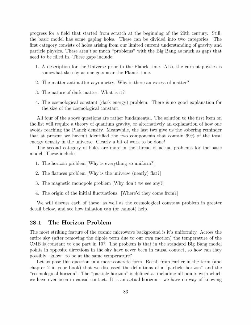
progress for a field that started from scratch at the beginning of the 20th century. Still,the basic model has some gaping holes. These can be divided into two categories. Thefirst category consists of holes arising from our limited current understanding of gravity andparticle physics. These aren’t so much “problems” with the Big Bang as much as gaps thatneed to be filled in. These gaps include:

1. A description for the Universe prior to the Planck time. Also, the current physics issomewhat sketchy as one gets near the Planck time.

2. The matter-antimatter asymmetry. Why is there an excess of matter?

3. The nature of dark matter. What is it?

4. The cosmological constant (dark energy) problem. There is no good explanation forthe size of the cosmological constant.

All four of the above questions are rather fundamental. The solution to the first item onthe list will require a theory of quantum gravity, or alternatively an explanation of how oneavoids reaching the Planck density. Meanwhile, the last two give us the sobering reminderthat at present we haven’t identified the two components that contain 99% of the totalenergy density in the universe. Clearly a bit of work to be done!

The second category of holes are more in the thread of actual problems for the basicmodel. These include:

1. The horizon problem [Why is everything so uniform?]

2. The flatness problem [Why is the universe (nearly) flat?]

3. The magnetic monopole problem [Why don’t we see any?]

4. The origin of the initial fluctuations. [Where’d they come from?]

We will discuss each of these, as well as the cosmological constant problem in greaterdetail below, and see how inflation can (or cannot) help.

28.1 The Horizon Problem

The most striking feature of the cosmic microwave background is it’s uniformity. Across theentire sky (after removing the dipole term due to our own motion) the temperature of theCMB is constant to one part in 104. The problem is that in the standard Big Bang modelpoints in opposite directions in the sky have never been in causal contact, so how can theypossibly “know” to be at the same temperature?

Let us pose this question in a more concrete form. Recall from earlier in the term (andchapter 2 in your book) that we discussed the definitions of a “particle horizon” and the“cosmological horizon”. The “particle horizon” is defined as including all points with whichwe have ever been in causal contact. It is an actual horizon – we have no way of knowing

83

anything about what is currently beyond the particle horizon. As we discussed previously,the particle horizon is defined as

RH = a∫ t

0

cdt

a. (481)

If the expansion of the universe at early times goes at a ∝ tβ, with β > 0, then

RH = tβ∫ t

0ct−βdt = (1− β)ct. (482)

and a particle horizon exists if β < 1.Using the same expansion form in the Friedmann equation,

a = −4

3πG

(

ρ+ 3p

c2

)

a, (483)

yieldsa = β(β − 1)tβ−2, (484)

and

β(β − 1) = −4

3πG

(

ρ+ 3p

c2

)

t2. (485)

The existence of an initial singularity requires a < 0 and hence 0 < β < 1. Combining thiswith the result above, we see that there must be a particle horizon.

How does the size of the particle horizon compare to the size of the surface of lastscattering? At zCMB = 1100, the CMB surface that we observe had a radius

rCMB =ctlookback1 + zCMB

≃ ct01 + zCMB

, (486)

so opposite directions in the sky show the CMB at sites that were 2rCMB apart at recom-bination. If the above is a bit unclear, the way to think about it is as follows. Consider usat the center of a sphere with the observed CMB emitted at a comoving distance from us ofctlookback. This is the radius above, with the (1 + z) included to convert to proper distance.

The size of the particle horizon at a given redshift for w = 0 is given by

RH ≃ 3ct ≃ 3ct0(1 + zCMB)−3/2 ≃ 3rCMB(1 + zCMB)−1/2 ≃ rCMB

10. (487)

The implication is that the CMB is homogeneous and isotropic on scales a factor of tenlarger than the particle horizon.

28.2 Inflation: Basic Idea

The most popular way of getting around the above problem is called inflation. The basic ideais to simply postulate that the universe underwent a period of accelerated expansion (a > 0)at early times. As we will see later, there are many variants of inflation, but they all boildown to the same result – a finite period of accelerated expansion very early. So how does

84

inflation help with the horizon problem? If there was a period of accelerated expansion, thenone can envision a scenario in which the entire observable universe was actually in causalcontact at some point prior to this accelerated expansion. In this case the uniformity of theCMB is no longer so mysterious. Let’s see how this would work.

28.2.1 Cosmological Horizon

When we discussed particle horizons early in the term, we also discussed the “cosmologicalhorizon”. This term is actually somewhat of a misnomer, but is commonly used. It’s not atrue horizon, but rather is simply defined as being equivalent to the Hubble proper distanceat a given redshift,

Rc = ca

a=

c

H(z), (488)

or a comoving distance

rc = ca0

a=c(1 + z)

H(z), (489)

which reduces to the familiarRc = rc ≡ DH =

c

H0(490)

at z = 0. The relevance of the cosmological horizon, or Hubble distance, is that physicalprocesses can keep things fairly homogeneous within a scale of roughly the cosmologicalhorizon. Recall during the thermodynamic discussion that reactions were in thermodynamicequilibrium if the collision time was less than the Hubble time; similarly, physically processescan act within regions less than the Hubble distance (cosmological horizon). There are acouple important things to remember about the cosmological horizon. First, objects can beoutside the cosmological horizon, but inside the particle horizon. Second, objects can movein and out of the cosmological horizon (unlike the particle horizon, where an object withinthe particle horizon will forever remain within the particle horizon).

[Those reading notes should now refer to figure 7.4 in book, as I will be drawing somethingsimilar on board.]

28.2.2 Inflationary solution

The horizon problem, as discussed above, is that points separated by proper distance l(comoving distance l0 = l(1 + z)) are only causally connected when l < RH , where RH isthe size of the particle horizon. If we consider a ∝ tβ at early times (with β < 1 as above),then the size of the horizon grows with time. Put simply, as the universe gets older light canreach farther so the particle horizon is larger.

Now, imagine that a region l0 that is originally within the cosmological horizon (l0 <rc(ti)) is larger than the horizon at some later time (l0 > rc(tf)). This can only happen ifthe comoving cosmological horizon decreases with time. In other words,

d

dt

ca0

a=−ca0a

a2< 0, (491)

85

or a > 0.The inflationary solution thus posits that the universe passes through a period of accel-

erated expansion, which after some time turns off and returns to a decelerated expansion.If observers (like us) are unaware of this period of accelerated expansion, then we perceivethe paradox of the horizon problem. The problem is non-existent though in the inflationarymodel because everything that we see was at some point in causal contact.

OK. That’s the basic picture. Now let’s work through the details. During the inflationaryera, we require that the Friedmann equation be dominated by a component with w < −1/3in order to have an accelerated expansion.

If we define the start and finish of the inflationary period as ti and tf , respectively, thenfrom the Friedmann equation we find,

(

a

ai

)2

= H2i

[

Ωi

(

aia

)1+3w

+ (1− Ωi)

]

(492)

≃ H2i

(

aia

)1+3w

(493)

a

a

(

a

ai

)−3(1+w)/2

= Hi (494)

where we have assumed Ωi ≃ 1 since we are considering early times. Now we have severalcases to consider. The first is w = −1. In this case, we have

da

a= Hidt, (495)

and integrating from ti to t we have,

a = aieHi(t−ti). (496)

This case is called “exponential inflation” for obvious reasons. Now, consider the cases wherew 6= 1. Starting from above and integrating again we now have,

d

da

[

−3(1 + w)

2

(

a

ai

)−3(1+w)/2]

=d

dt(Hit) (497)

−3(1 + w)

2

[

1−(

a

ai

)3(1+w)/2]

= Hi(t− ti (498)

(

a

ai

)3(1+w)/2

=2

3(1 + w)Hi(t− ti) + 1 (499)

a ≃ ai

[

1 +Hi(t− ti)

q

]q

; where q =2

3(1 + w). (500)

For −1 < w < −1/3 and t/ti > 1, this equation reduces to simply

a ∝ tq; where q > 1. (501)

86

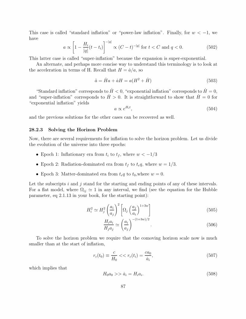
This case is called “standard inflation” or “power-law inflation”. Finally, for w < −1, wehave

a ∝[

1− Hi

|q| (t− ti)]−|q|

∝ (C − t)−|q| for t < C and q < 0. (502)

This latter case is called “super-inflation” because the expansion is super-exponential.An alternate, and perhaps more concise way to understand this terminology is to look at

the acceleration in terms of H. Recall that H = a/a, so

a = Ha + aH = a(H2 + H) (503)

“Standard inflation” corresponds to H < 0, “exponential inflation” corresponds to H = 0,and “super-inflation” corresponds to H > 0. It is straightforward to show that H = 0 for“exponential inflation” yields

a ∝ eHit, (504)

and the previous solutions for the other cases can be recovered as well.

28.2.3 Solving the Horizon Problem

Now, there are several requirements for inflation to solve the horizon problem. Let us dividethe evolution of the universe into three epochs:

• Epoch 1: Inflationary era from ti to tf , where w < −1/3

• Epoch 2: Radiation-dominated era from tf to teq, where w = 1/3.

• Epoch 3: Matter-dominated era from teq to t0,where w = 0.

Let the subscripts i and j stand for the starting and ending points of any of these intervals.For a flat model, where Ωij ≃ 1 in any interval, we find (see the equation for the Hubbleparameter, eq 2.1.13 in your book, for the starting point):

H2i ≃ H2

j

(

aiaj

)2 [

Ωj

(

ajai

)1+3w]

(505)

HiaiHjaj

≃(

aiaj

)−(1+3w)/2

. (506)

To solve the horizon problem we require that the comoving horizon scale now is muchsmaller than at the start of inflation,

rc(t0) ≡c

H0

<< rc(ti) =ca0

ai, (507)

which implies thatH0a0 >> ai = Hiai. (508)

87

Consequently, this means that

HiaiHfaf

<<H0a0

Hfaf=

H0a0

Heqaeq

HeqaeqHfaf

, (509)

which gives

(

aiaf

)−(3w+1)/2

<<

(

a0

aeq

)−1/2 (aeqaf

)−1

(510)

(

afai

)−(3w+1)

>>

(

a0

aeq

)(

aeqaf

)2

(511)

If one substitutes in a0/aeq = (1 + zeq)−1, and

aeqaf

=1 + zeq1 + zf

=TfTeq

, (512)

taking Teq ≃ 10−30TP , where TP is the Planck temperature, this yields

(

afai

)−(1+3w)

>> 1060(1 + zeq)−1(

TfTP

)2

. (513)

Consequently, for an exponential expansion this implies that the number of e-foldings is

N ≡ ln(af/ai) >> 60

[

ln 10 + ln(Tf/TP )/30− ln(1 + zeq)/60

|1 + 3w|

]

. (514)

For most proposed models, 10−5 < Tf/TP < 1, which means that we require N >> 60.Think about this for a moment. This says that the universe had to grow by a factor of

at least e60 during inflation, or a factor of 1026. As we shall see in a moment, this likelywould have to happen during a time interval of order 10−32s. As an aside, note that whilethe expansion rate is >> c, this does not violate standard physics since it is spacetime ratherthan matter/radiation undergoing superluminal motion. Any particle initially at rest in thespacetime remains at rest and just sees everything redshift away.

28.3 Inflation and the Monopole Problem

Let’s now see how inflation helps (or fails to help) some of the other problems. One problemwith the basic Big Bang model is that most grand unification theories (GUTs) in particlephysics predict that magnetic defects are formed when the strong and electroweak forcesdecouple. In the most simple case these defects are magnetic monopoles – analogous toelectrons and positrons, but with a magnetic rather than electric charge.

From these theories one finds that magnetic monopoles should have a charge that is amultiple of the Dirac charge, gD, such that

gM = ngD = n68.5e, (515)

88

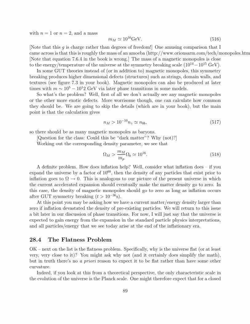
with n = 1 or n = 2, and a massmM ≃ 1016GeV. (516)

[Note that this g is charge rather than degrees of freedom!] One amusing comparison that Icame across is that this is roughly the mass of an amoeba (http://www.orionsarm.com/tech/monopoles.html).[Note that equation 7.6.4 in the book is wrong.] The mass of a magnetic monopoles is closeto the energy/temperature of the universe at the symmetry breaking scale (1014−1015 GeV).

In some GUT theories instead of (or in addition to) magnetic monopoles, this symmetrybreaking produces higher dimensional defects (structures) such as strings, domain walls, andtextures (see figure 7.3 in your book). Magnetic monopoles can also be produced at latertimes with m ∼ 105 − 1012 GeV via later phase transitions in some models.

So what’s the problem? Well, first of all we don’t actually see any magnetic monopolesor the other more exotic defects. More worrisome though, one can calculate how commonthey should be. We are going to skip the details (which are in your book), but the mainpoint is that the calculation gives

nM > 10−10nγ ≃ n0b, (517)

so there should be as many magnetic monopoles as baryons.[Question for the class: Could this be “dark matter”? Why (not)?]Working out the corresponding density parameter, we see that

ΩM >mM

mpΩb ≃ 1016. (518)

A definite problem. How does inflation help? Well, consider what inflation does – if youexpand the universe by a factor of 1060, then the density of any particles that exist prior toinflation goes to Ω → 0. This is analogous to our picture of the present universe in whichthe current accelerated expansion should eventually make the matter density go to zero. Inthis case, the density of magnetic monopoles should go to zero as long as inflation occursafter GUT symmetry breaking (t > 10−36s).

At this point you may be asking how we have a current matter/energy density larger thanzero if inflation devastated the density of pre-existing particles. We will return to this issuea bit later in our discussion of phase transitions. For now, I will just say that the universe isexpected to gain energy from the expansion in the standard particle physics interpretations,and all particles/energy that we see today arise at the end of the inflationary era.

28.4 The Flatness Problem

OK – next on the list is the flatness problem. Specifically, why is the universe flat (or at leastvery, very close to it)? You might ask why not (and it certainly does simplify the math),but in truth there’s no a priori reason to expect it to be flat rather than have some othercurvature.

Indeed, if you look at this from a theoretical perspective, the only characteristic scale inthe evolution of the universe is the Planck scale. One might therefore expect that for a closed

89

universe the lifetime might be tu ≃ tP . Similarly, for an open universe one would expect thecurvature to dominate after roughly a Planck time. Clearly not the case in reality!

Let’s start by quantifying how flat the universe is. We’ll do this for a model without acosmological constant, but the same type of derivation is possible (with a bit more algebra)for a more general model. We can rearrange the Friedmann equation,

a2 − 8πG

3ρa2 = −Kc2, (519)

to find(

a

a

)2

− 8πG

3ρ = −Kc

2

a2(520)

H2(1− ρ/ρc) = −Kc2

a2(521)

H2(1− Ω)a2 = −Kc2 (522)

H2 ρ

ρc

(

1− Ω

Ω

)

a2 = −Kc2 (523)

(Ω−1 − 1)ρa2 =−Kc238πG

= constant (524)

so(Ω−1 − 1)ρa2 = (Ω−1

0 − 1)ρ0a20. (525)

We can put this in terms of more observable parameters. Since we know that ρ ∝ a−4

for the radiation-dominated era and ρ ∝ a−3 for the matter-dominated era, we can use theabove to solve for the density parameter at early times. Specifically

(Ω−1 − 1)ρa2 = (Ω−1eq − 1)ρeqa

2eq; (526)

and

(Ω−1eq − 1)ρeqa

2eq = (Ω−1

0 − 1)ρ0a20 (527)

So

(Ω−1 − 1)

(

a

aeq

)−2

= (Ω−1eq − 1) (528)

(Ω−1eq − 1) = (Ω−1

0 − 1)a0

aeq(529)

(530)

and therefore

Ω−1 − 1

Ω−10 − 1

=(

aeqa

)2(

a0

aeq

)

= (1 + zeq)−1(

TeqT

)2

≃ 10−60(

TPT

)2

. (531)

Consequently, even for an open model with Λ = 0, Ω0 = 0.3, the above result requires thatΩ−1P − 1 ≤ 10−60 at the Planck time. Indeed, right now we know that Ω0 + ΩΛ = 1.02± 0.02

(WMAP, Spergel et al. 2003), which further tightens the flatness constraint in the Planckera.

90

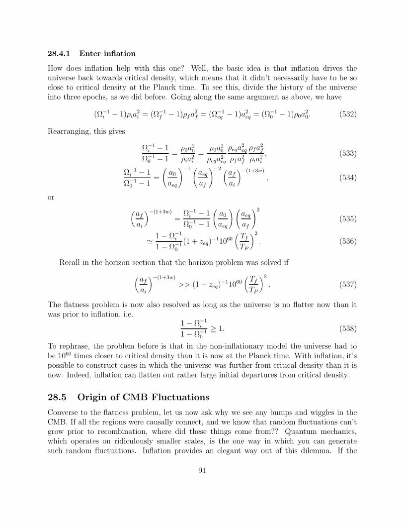
28.4.1 Enter inflation

How does inflation help with this one? Well, the basic idea is that inflation drives theuniverse back towards critical density, which means that it didn’t necessarily have to be soclose to critical density at the Planck time. To see this, divide the history of the universeinto three epochs, as we did before. Going along the same argument as above, we have

(Ω−1i − 1)ρia

2i = (Ω−1

f − 1)ρfa2f = (Ω−1

eq − 1)a2eq = (Ω−1

0 − 1)ρ0a20. (532)

Rearranging, this gives

Ω−1i − 1

Ω−10 − 1

=ρ0a

20

ρia2i

=ρ0a

20

ρeqa2eq

ρeqa2eq

ρfa2f

ρfa2f

ρia2i

, (533)

Ω−1i − 1

Ω−10 − 1

=

(

a0

aeq

)−1 (aeqaf

)−2 (afai

)−(1+3w)

, (534)

or

(

afai

)−(1+3w)

=Ω−1i − 1

Ω−10 − 1

(

a0

aeq

)(

aeqaf

)2

(535)

≃ 1− Ω−1i

1− Ω−10

(1 + zeq)−11060

(

TfTP

)2

. (536)

Recall in the horizon section that the horizon problem was solved if

(

afai

)−(1+3w)

>> (1 + zeq)−11060

(

TfTP

)2

. (537)

The flatness problem is now also resolved as long as the universe is no flatter now than itwas prior to inflation, i.e.

1− Ω−1i

1− Ω−10

≥ 1. (538)

To rephrase, the problem before is that in the non-inflationary model the universe had tobe 1060 times closer to critical density than it is now at the Planck time. With inflation, it’spossible to construct cases in which the universe was further from critical density than it isnow. Indeed, inflation can flatten out rather large initial departures from critical density.

28.5 Origin of CMB Fluctuations

Converse to the flatness problem, let us now ask why we see any bumps and wiggles in theCMB. If all the regions were causally connect, and we know that random fluctuations can’tgrow prior to recombination, where did these things come from?? Quantum mechanics,which operates on ridiculously smaller scales, is the one way in which you can generatesuch random fluctuations. Inflation provides an elegant way out of this dilemma. If the

91

universe expanded exponentially, any quantum fluctuations in the energy density during theexpansion are magnified to macroscopic scales. Since quantum wavefunctions are gaussian,inflation makes the testable prediction that CMB fluctuations should be gaussian as well.This is the one currently testable prediction of inflation, and it appears that the fluctuationsare indeed gaussian. We’ll talk more about these later.

28.6 The Cosmological Constant Problem: First Pass

Why is there a non-zero cosmological constant that has a value anywhere near the criticaldensity? This is the basic question. We will return to this in greater detail after ourdiscussion of phase transitions, but the basic problem is that current particle physics predictsa cosmological constant (if non-zero) that’s off by about 110 orders of magnitude. Inflationdoes not help with this one at all.

28.7 Constraints on the epoch of inflation

Most theories predict that inflation should have occurred at t = 10−36 − 10−32s. Inflationmust occur no earlier than 10−36s, which is the GUT time, or else we should see magneticmonopoles or related topological defects. The end time constraint is more nebulous – itsimply must have lasted at least until 10−32s for a 1060 increase in the scale factor.

29 The Physics of Inflation

In the previous section we have motivated why a period of accelerated expansion in the earlyuniverse would be a nice thing to have. Now how would one physically achieve such a state?This question is in fact even more relevant that it was even 10 years ago, as we now know thatthe universe is currently in the early stage of another accelerated (inflationary!) expansion.We will not go through all the details, but will qualitatively describe the fundamental (andpartially speculative) physics.

29.1 Phase Transitions

Most of you are familiar with the concept of a phase transition in other contexts. Phasetransitions are defined by abrupt changes in one or more of the physical properties of asystem when some variable (temperature) is changed slightly. Examples of well-known phasetransitions include:

• Freezing and boiling (transformation from the liquid to solid and gas phases).

• Magnetism – materials are ferromagnetic below the Curie temperature, but lose theirferromagnetism above this temperature

92

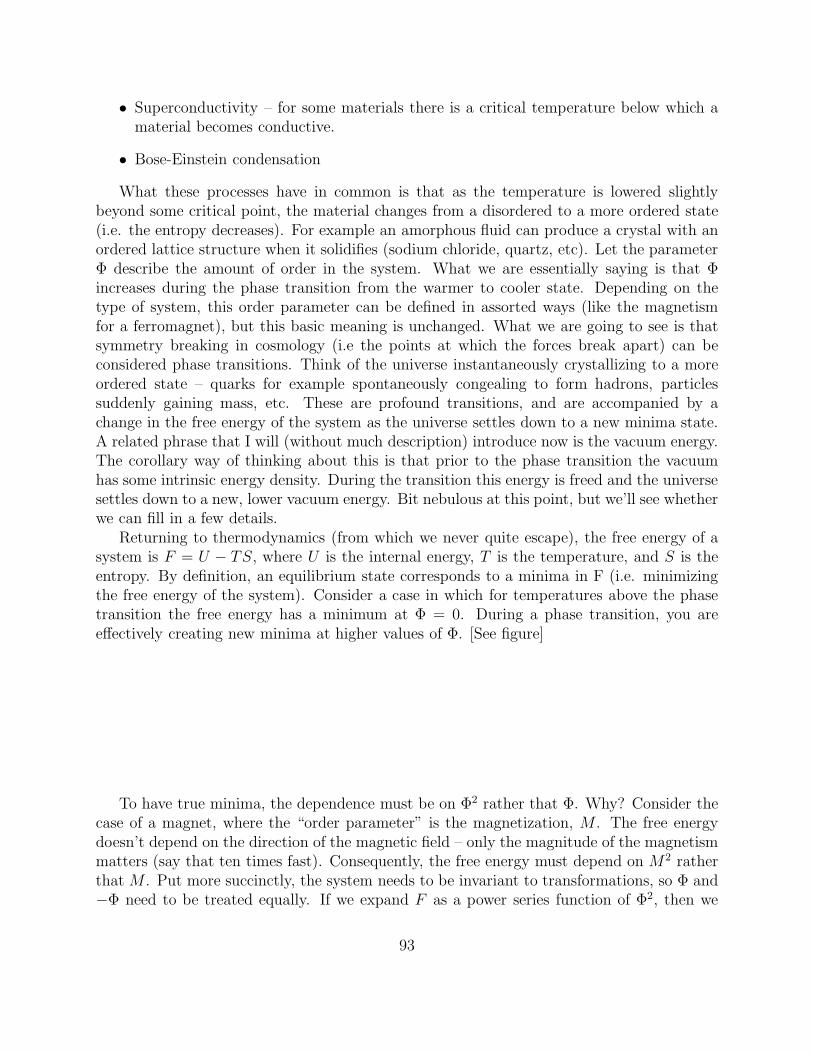
• Superconductivity – for some materials there is a critical temperature below which amaterial becomes conductive.

• Bose-Einstein condensation

What these processes have in common is that as the temperature is lowered slightlybeyond some critical point, the material changes from a disordered to a more ordered state(i.e. the entropy decreases). For example an amorphous fluid can produce a crystal with anordered lattice structure when it solidifies (sodium chloride, quartz, etc). Let the parameterΦ describe the amount of order in the system. What we are essentially saying is that Φincreases during the phase transition from the warmer to cooler state. Depending on thetype of system, this order parameter can be defined in assorted ways (like the magnetismfor a ferromagnet), but this basic meaning is unchanged. What we are going to see is thatsymmetry breaking in cosmology (i.e the points at which the forces break apart) can beconsidered phase transitions. Think of the universe instantaneously crystallizing to a moreordered state – quarks for example spontaneously congealing to form hadrons, particlessuddenly gaining mass, etc. These are profound transitions, and are accompanied by achange in the free energy of the system as the universe settles down to a new minima state.A related phrase that I will (without much description) introduce now is the vacuum energy.The corollary way of thinking about this is that prior to the phase transition the vacuumhas some intrinsic energy density. During the transition this energy is freed and the universesettles down to a new, lower vacuum energy. Bit nebulous at this point, but we’ll see whetherwe can fill in a few details.

Returning to thermodynamics (from which we never quite escape), the free energy of asystem is F = U − TS, where U is the internal energy, T is the temperature, and S is theentropy. By definition, an equilibrium state corresponds to a minima in F (i.e. minimizingthe free energy of the system). Consider a case in which for temperatures above the phasetransition the free energy has a minimum at Φ = 0. During a phase transition, you areeffectively creating new minima at higher values of Φ. [See figure]

To have true minima, the dependence must be on Φ2 rather that Φ. Why? Consider thecase of a magnet, where the “order parameter” is the magnetization, M . The free energydoesn’t depend on the direction of the magnetic field – only the magnitude of the magnetismmatters (say that ten times fast). Consequently, the free energy must depend on M2 ratherthat M . Put more succinctly, the system needs to be invariant to transformations, so Φ and−Φ need to be treated equally. If we expand F as a power series function of Φ2, then we

93

can writeF (Φ) ≈ F0 + AΦ2 +Bφ4. (539)

If A > 0 and B > 0, then we have a simple curve with the minima at Φ = 0 – i.e. theminimum is in the most disordered state. On the other hand, if A < 0 and B > 0, thenyou can create new minima at more ordered states. If you think of the free energy plot as apotential well, you can see that the phase transition changes the potential and the universeshould roll down to the new minima.

How would you change from one curve to another? Consider the case in which A =K(T −Tc). In this case, the sign of A changes when you drop below the critical temperature,and as you go to lower temperatures the free energy minima for the ordered states get lowerand lower. This type of transition is a second order phase transition. As you can seefrom a time sequence, the transition is smooth between T > Tc and T < Tc and the processis transition is gradual as the system slowly rolls towards the new minima.

As an alternative, there are also first-order phase transitions. In first-order transitionsthe order parameter appears rapidly and the difference in free-energy above and below thecritical temperature is finite rather than infinitesimal. In other words, there is a sharpchange in the minimum free energy right at the critical temperature. The finite change inthe free energy at this transition, ∆F , is the latent heat of the transition (sound familiarfrom chemistry?).

Lets look at an example of such a transition. Consider the figure below, in which thereare initially two local minima for T > Tc. As the system cools, these become global minimaat T = TC , but the system has no way of reaching these minima. At some later time,after the system has cooled further, it becomes possible for the system to transition to themore ordered state (either by waiting until the barrier is gone, or via quantum tunnelingdepending on the type of system. In this case, the system rapidly transitions to the newminima and releases the latent heat associated with the change in free energy. This processis supercooling. From a mathematical perspective, one example (as shown in the figure)can be achieved by making the dependence,

F = F0 + AΦ2 + C|Φ|3 +BΦ4, (540)

with A > 0, B > 0, and C < 0.

29.2 Cosmological Phase Transitions

So how does freezing water relate to cosmology? The basic idea is that the Universe under-goes cosmological phase transitions. You may recall that we have used the term “spontaneoussymmetry breaking” in describing the periods during which the fundamental forces separate.From the particle physics perspective, these events correspond to phase transitions in whichthe universe moves from a disordered to a more ordered state (for instance particles acquir-ing mass, and differentiation of matter into particles with unique properties like quarks andleptons). The free energy in this interpretation corresponds to a vacuum energy contained

94

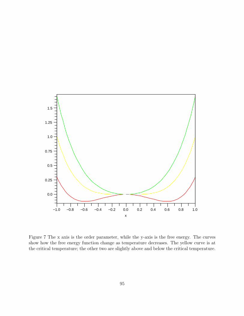
x

1.0

0.5

0.8

0.0

1.5

1.25

0.75

1.0

0.25

0.60.40.20.0−0.2−0.4−0.6−0.8−1.0

Figure 7 The x axis is the order parameter, while the y-axis is the free energy. The curvesshow how the free energy function change as temperature decreases. The yellow curve is atthe critical temperature; the other two are slightly above and below the critical temperature.

95

−0.3

x

0.5−0.5

0.1

1.00.0

−0.1

−1.0

−0.2

0.2

0.0

−0.4

Figure 8 Similar to previous figure, except that this one shows an example of supercooling(first-order phase transition). In this case, there is a barrier that prevents the system frommoving to the new minimum until T << TC , at which point it rapidly transitions to the newstate and releases latent heat.

96

in some scalar field (referred to as the inflaton field for inflation) – which is equivalent tothe order parameter that we have been discussing (again for reference, temperature is anexample of a scalar field while gravity is an example of a vector field). During the phasetransition this vacuum energy decreases. Note that there are also other phase transitionsin the early universe not associated directly with spontaneous symmetry breaking (think ofthe quarks congealing into hadrons for instance). As we shall discuss soon, this vacuum en-ergy can potentially drive a period of inflationary expansion if it dominates the total energydensity. Meanwhile, the latent heat released during the phase transition is also key.

So when during the early universe are cosmological phase transitions possible? Well,basically most of the time, as the constituents in the universe are rapidly evolving and new,more ordered structures are forming. The most dramatic phase transitions correspond tothe spontaneous symmetry breaking scales when the forces separate, but it is possible tohave other phase transitions along the way. Your book attempts to divide this time up untilthe quark-hadron transition into intervals characterized by the types of phase transitionsoccurring at each epoch. This is a reasonable approach, and we shall review these periodshere.

• The Planck Time (∼ 1019 GeV) – This is the point at which we require a quantumtheory of gravity, and for which any super grand unification theory must unify gravitywith the other forces above this temperature.

• GUT (∼ 1015 GeV) – This is the temperature at which the strong and electroweakforces break apart. The GUT scale is when magnetic monopoles are expected to form,so we require a period of inflation during or after this epoch. We want inflation tooccur very near this epoch though, because only at and above this temperature domost current models permit creation of a baryon-antibaryon asymmetry. This is nota hard constraint though, as it is possible to construct scenarios in which baryonconservation is violated at somewhat lower temperatures.

• Between the GUT and Electroweak scales. The main point in the book is that thetimescale between GUT and Electroweak is from 10−37−10−11s, which logarithmicallyleaves a lot of time for other phase transitions to occur. These phase transitions wouldnot be associated with symmetry breaking.

• Electroweak scale to quark-hadron transition. The universe undergoes a phase tran-sition when the weak and electromagnetic forces split. It’s at this point that leptonsacquire mass incidentally. Also in this category is the (much lower temperature) quark-hadron transition, at which free quarks are captured into hadrons.

Any and all of the above transitions can yield a change in the vacuum energy. Not allof the above however can cause inflation. Keep in mind as we go along that for inflation tooccur, the vacuum energy must dominate the total energy density.

97

29.3 Return to the Cosmological Constant Problem

As promised, we’re now going to finish up talking about the cosmological constant problem– specifically the problem of how it can be non-zero and small. Recall that the densitycorresponding to the cosmological constant (WMAP value) is given by

|ρΛ| = 0.7× Λc2

8πG= 1.4× 10−29 gcm−3 ≃ 10−48GeV4. (541)

Equivalently, one can compute the value of Λ, finding Λ = 10−55cm−2.Small numbers, but is this a problem? The cosmological constant is often interpreted as

corresponding to the vacuum energy of some scalar field. This is analogous to the discussionof free energy that we saw in previous sections. Modern gauge theories in particle physicspredicts this vacuum energy corresponds to an effective potential,

ρv ≈ V (Φ, T ), (542)

and that the drop in the vacuum energy at a phase transition should be of the order

∆ρv ≈m4

(hc)3, (543)

where m is the mass scale of the relevant phase transition. This density change correspondsto 1060 GeV4 for the GUT scale and values of 10−4 − 1012 GeV4 for other transitions (likethe electroweak).

Now, if we take all the phase transitions together, this says that

ρv(tP lanck) = ρv(t0) +∑

i

∆ρv(mi) ≈ 10−48 + 1060 GeV4 =∑

i

∆ρv(mi)(1 + 10−108). (544)

In other words, starting with the vacuum density before GUT, the current vacuum densityis a factor of 10108 smaller – and this value is very close to the critical density. Your bookregards this as perhaps the most serious problem in all of cosmology. What is a greatermystery I would argue is why we find ourselves at a point in the history of the universeduring which we are just entering a new inflationary phase.

29.4 Inflation: Putting the Pieces Together

We’ve now defined inflation in terms of its impact upon the growth of the scale factor (a > 0),explored how it can resolve some key problems with the basic big bang, and done a bit ofbackground regarding phase transitions. Seems like a good idea, so time to start assemblinga coherent picture of how one might incorporate inflation into the Big Bang model. At avery basic level, all inflationary models have the following properties:

• There must be an epoch in the early universe in which the vacuum energy density,ρ ∝ V (Φ), dominates the total energy density.

98

• During this epoch the expansion is accelerated, which drives the radiation and matterdensity to zero.

• Vacuum energy is converted into matter and radiation as Φ oscillates about the newminima. This reheats the universe back to a value near the value prior to inflation,with all previous structure having been washed out.

• This must occur during or after the GUT phase to avoid topological defects. (note:some versions don’t address this directly)

We will now consider the physics of general inflationary models and then discuss a fewof the zoo of different flavors of inflation. For a scalar field Φ, the Lagrangian of the field is

LΦ =1

2Φ2 − V (Φ, T ), (545)

analogous to classical mechanics. Note that the scalar field Φ is the same as the orderparameter that we have been discussing and the potential V is analogous to the free energy.The density associated with this scalar field is

ρΦ =1

2Φ2 + V (Φ, T ) (546)

(547)

Consider the case of a first-order phase transition (supercooling). In this case, the phasetransition does not occur until some temperature Tb < Tc, at which point Φ assumes thenew minimum value. If this transition is assumed to occur via either quantum tunneling orthermal fluctuations (rather than elimination of the barrier), then the transition will occurin a spatially haphazard fashion. In other words, the new phase will appear as nucleatingbubbles in the false vacuum, which will grow until the entire Universe has settled to the newvacuum.

On the other hand, if the transition is second order, the process is more uniform asall regions of space descend to the new minima simultaneously. Note however that not alllocations will descend to the same minima, so you will end up with “bubbles” or domains.The idea is that one such bubble should eventually encompass our portion of the Universe.

Now, how does this evolution occur? We’ll phrase this in terms of the equation of motionfor the scalar field,

d

dt

∂LΦa3

∂Φ− ∂LΦa

3

∂Φ= 0, (548)

which, using the Lagrangian above,

Φ + 3a

aΦ +

∂V (Φ)

∂Φ= 0 (549)

Let’s look at this above equation. If we ignore the a term, then this is equivalent to aball oscillating back and forth in the bottom of a potential well. In this analogy, the 3a/a

99

term then corresponds to friction damping the kinetic energy of the ball. It is standard ininflation to speak of the vacuum as “rolling down” to the new minima. More specifically, atthe start of inflation one normally considers what is called the “slow roll phase”, in whichthe kinetic energy is << the potential energy. This corresponds to the case in which themotion is friction dominated, so the ball slowly moves down to the new minima.

Remember that inflation causes ρr and ρm to trend to zero, so the Friedmann equationduring the phase transition is approximately,

(

a

a

)2

=8πGρΦ

3=

8πG

3

(

1

2Φ2 + V (Φ, T )

)

. (550)

In the slow roll phase, this reduces to

(

a

a

)2

=8πG

3V (Φ, T ), (551)

soa ∝ exp(t/τ), (552)

where

τ ≃[

3

8πGV

]1/2

. (553)

For most models the above timescale works out to roughly τ = 10−34 s. Since we needa minimum of 60 e-foldings to solve the horizon problem, this means that the inflationaryperiod should last for at least 10−32 s. Note that this assumes inflation starts right at thephase transition. It’s possible to have ongoing inflation for a while before this, but you stillwant to have a large number of e-foldings to get rid of monopoles and other relics producedat the GUT temperature.

As the roll down to the new minimum proceeds, the field eventually leaves the slowroll phase and rapidly drops down towards, and oscillates about the new minima. Theseoscillations are damped by the creation of new particles (i.e. conversion of the vacuumenergy into matter and radiation). Mathematically, this corresponds to the addition of adamping term in the equation of motion

Φ + 3a

aΦ + ΓΦ +

∂V (Φ)

∂Φ= 0. (554)

Physically, this has the effect of reheating the universe back up to some temperature,T < Tcrit, after which we proceed with a normal Big Bang evolution. Note that this newtemperature has to be sufficiently high for baryosynthesis.

So to summarize, the best way to look at things is like this:

1. Vacuum energy starts to dominate, initiating an inflationary expansion.

2. Inflation cools us through a phase transition, which initiates a slow roll down to thenew minima. Inflation continues during this epoch.

100

3. Slow roll phase ends and vacuum drops to new minima. Inflation ends.

4. Scalar field oscillates around this new minima, releasing energy via particle productionuntil it settles into the new minima. This released energy reheats the universe.

5. Back to the way things were before the inflationary period.

29.5 Types of Inflation

OK - so what are the types of inflation. Inflation as a topic could fill the better part of asemester, with much of the time devoted to the various flavors. Here I am aiming to providejust an overview of inflation, and will continue that theme with a sparse sampling of typesof inflation.

29.5.1 Old Inflation

The original inflationary model (Guth, 1981) suggested that inflation is associated with afirst-order phase transition. As we discussed, a first-order phase transition implies a spatiallyhaphazard transition. It turns out that the bubbles produced in this way are too small forour Universe and never coalesce into a larger bubble, so this model was quickly abandoned.

29.5.2 New Inflation

Shortly after the work by Guth, Andre Linde (1982) proposed a new version with a second-order rather than first-order phase transition. It turns out that a second order transitionleaves larger spatial domains, and enables the entire universe to be in a single bubble withthe same value of Φ. New inflation has several problems though that inspired other versions.(see your book for details)

29.5.3 Chaotic Inflation

Chaotic inflation (Linde 1983) was an interesting revision in that it does not require anyphase transitions. Instead, the idea is that near the Planck time Φ (whatever it is) variesspatially. Consider an arbitrary potential V(Φ) with the one condition that the minimumis at Φ = 0. Now, take a patch of the universe with a large, non-zero value of Φ. Clearly,within this region Φ will evolve just as it would right after a second-order phase transition– starting with a slow roll and eventually reheating and settling into the minima.

The mathematics is the same as before – the main difference now is that we’ve removedthe connection between inflation and normal particle physics. It’s completely independentof GUT or any other phase transitions.

101

29.5.4 Stochastic Inflation

Stochastic, or eternal, inflation is an extension of chaotic inflation. Starting with an inhomo-geneous universe, the stochastic model incorporates quantum fluctuations as Φ evolves. Thebasic idea then is that there are always portions of the universe entering the inflationaryphase, so you have many independent patches of universe that inflate at different times.What’s kind of interesting about this approach is that it brings us full circle to the SteadyState model in the sense that there is no overall beginning or end – just an infinite numberof Hubble patches evolving separately infinitely into the future.

102

30 Cosmic Microwave Background

[Chapter 17]It is now time to return for a more detailed look at the cosmic microwave background –

although not as detailed a look as one would like due to time constraints on this class. Weare now in what should be considered the “fun” part of the term – modern cosmology andissues that remain relevant/open at the present time. Let us start with a qualitative lookat the CMB and how the encoded information can be represented. We will then discuss theunderlying physics in greater detail and play with some animations and graphics on WayneHu’s web page.

30.1 Extracting information from the CMB

The structure observed in the CMB, as we will see, is a veritable treasure trove of information.It provides a picture of the matter distribution at the epoch of recombination, constrainsa host of cosmological parameters, and provides information on assorted physics that hasoccurred subsequent to recombination (such as the epoch of reionization). Before we get tothe physics though, a first question that we will discuss is now one might go about extractingthe essential information from a 2-d map of the CMB sky.

The standard approach is to parameterize the sky map in terms of spherical harmonics,such that

∆T

< T >≡ T− < T >

< T >=

∞∑

l=0

l∑

m=−l

almYlm(θ, φ), (555)

where the Ylm are the standard spherical harmonics familiar from quantum mechanics or(helio)seismology

Ylm(θ, φ) =

[

2l + 1

4π

(l −m)!

(l +m)!

]1/2

Pml (cosθ)eimφ, (556)

with the Pml being Legendre polynomials,

Pml (cos θ) =

(−1)m

2ll!

(

1− cos2 θ)m/2 dl+m

d cosl+m θ

(

cos2 θ − 1)l

(557)

Now, for a given map the coefficients alm are not guaranteed to be real – in general they willbe complex numbers. Rather, the more physical quantity to consider is the power in eachmode, which is defined as

Cl ≡< |alm|2 > . (558)

As we will see in a moment, the angular power spectrum, measured in terms of Cl, is thefundamental observable for CMB studies. Specifically, when we see a typical angular powerspectrum for the CMB, the y axis is given by [l(l+1)Cl/(2π)]1/2. The units are µK, and thiscan physically thought of as the amplitude of temperature fluctuations ∆T/T for a givenangular scale, appropriately normalized.

103

First though, let’s consider the physical interpretation of different l modes. The l = 0mode corresponds to a uniform offset in temperature, and thus can be ignored. The l = 1mode is dipole mode. This term, which for the CMB is several orders of magnitude largerthan any other terms, is interpreted as being due to our motion relative to the CMB.

How does this effect the temperature? Assume that our motion is non-relativistic (whichis the case). In this case, the observed frequency of the CMB is shifted by a factor ν ′ =ν(1 + βcosθ), where β = v/c and θ = 0 is defined as the direction of our motion relative tothe CMB. For a black-body spectrum it can be shown that this corresponds to a temperaturedistribution,

T (θ) = T0(1 + β cos θ). (559)

Thus, the lowest order anisotropy in the CMB background tells us our velocity (bothspeed and direction) relative to the microwave background, and hence essentially relative tothe cosmic rest frame. Not a bad start.

Moving beyond the dipole mode, the l ≥ 2 modes are due primarily to intrinsic anisotropyproduced either at recombination or by subsequent physics. These are the modes that wecare most about. The book provides a rough guide that the angular scale of fluctuations forlarge values of l is θ ≃ 60/l – more useful and correct numbers to keep in mind are thatl = 10 corresponds to about 10 and l = 100 to about 1.

30.2 Physics

See http://background.uchicago.edu/whu/intermediate/intermediate.htmlThe quick summary is that the peaks in the CMB angular power spectrum are due

to acoustic oscillations in the plasma at recombination. The first peak corresponds to afundamental mode with size equal to the sound horizon at recombination, while the higherorder peaks are harmonics of this fundamental mode. The location of the first peak dependsupon the angular diameter distance to the CMB, and is consequently determined primarilyby the spatial curvature (with some dependence upon Λ). The relative amplitude of thesecond peak constrains the baryon density, while the third peak can be used to measurethe total matter density. Meanwhile, the damping tail provides a cross-check on the abovemeasurements. Finally, if it can be measured the polarization provides a means of separatingthe effects of reionization epoch and gravitational waves. Note that the currently measuredpower spectrum of temperature fluctuations is commonly referred to as the scalar powerspectrum (since temperature is a scalar field). Polarization on the other hand also probesthe tensor and vector power spectrum.

30.3 CMB Polarization and Inflation

[see section 13.6 in your book] One of the predictions of inflation is the presence of gravita-tional waves, which alter the B-mode of the CMB tensor power spectrum. If one can measurethis polarization, then one can constrain the nature of the inflation potential. Consider the

104

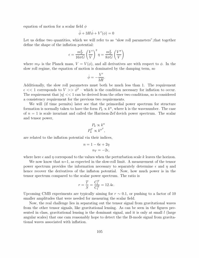
equation of motion for a scalar field φ

φ+ 3Hφ+ V ′(φ) = 0

Let us define two quantities, which we will refer to as “slow roll parameters”,that togetherdefine the shape of the inflation potential:

ǫ =m2P

16πG

(

V ′

V

)2

η =m2P

8πG

(

V ′′

V

)

where mP is the Planck mass, V = V (φ), and all derivatives are with respect to φ. In theslow roll regime, the equation of motion is dominated by the damping term, so

φ = − V ′

3H.

Additionally, the slow roll parameters must both be much less than 1. The requirementǫ << 1 corresponds to V >> φ2 – which is the condition necessary for inflation to occur.The requirement that |η| << 1 can be derived from the other two conditions, so is considereda consistency requirement for the previous two requirements.

We will (if time permits) later see that the primordial power spectrum for structureformation is normally taken to have the form Pk ∝ kn, where k is the wavenumber. The caseof n = 1 is scale invariant and called the Harrison-Zel’dovich power spectrum. The scalarand tensor power,

Pk ∝ kn

P Tk ∝ kn

T

,

are related to the inflation potential via their indices,

n = 1− 6ǫ+ 2η

nT = −2ǫ,

where here ǫ and η correspond to the values when the perturbation scale k leaves the horizon.We now know that n=1, as expected in the slow-roll limit. A measurement of the tensor

power spectrum provides the information necessary to separately determine ǫ and η andhence recover the derivatives of the inflaton potential. Now, how much power is in thetensor spectrum compared to the scalar power spectrum. The ratio is

r =T

S=CTl

CSl

= 12.4ǫ.

Upcoming CMB experiments are typically aiming for r ∼ 0.1, or pushing to a factor of 10smaller amplitudes that were needed for measuring the scalar field.

Now, the real challenge lies in separating out the tensor signal from gravitational wavesfrom the other tensor signals, like gravitational lensing. As can be seen in the figures pre-sented in class, gravitational lensing is the dominant signal, and it is only at small l (largeangular scales) that one cam reasonably hope to detect the the B-mode signal from gravita-tional waves associated with inflation.

105

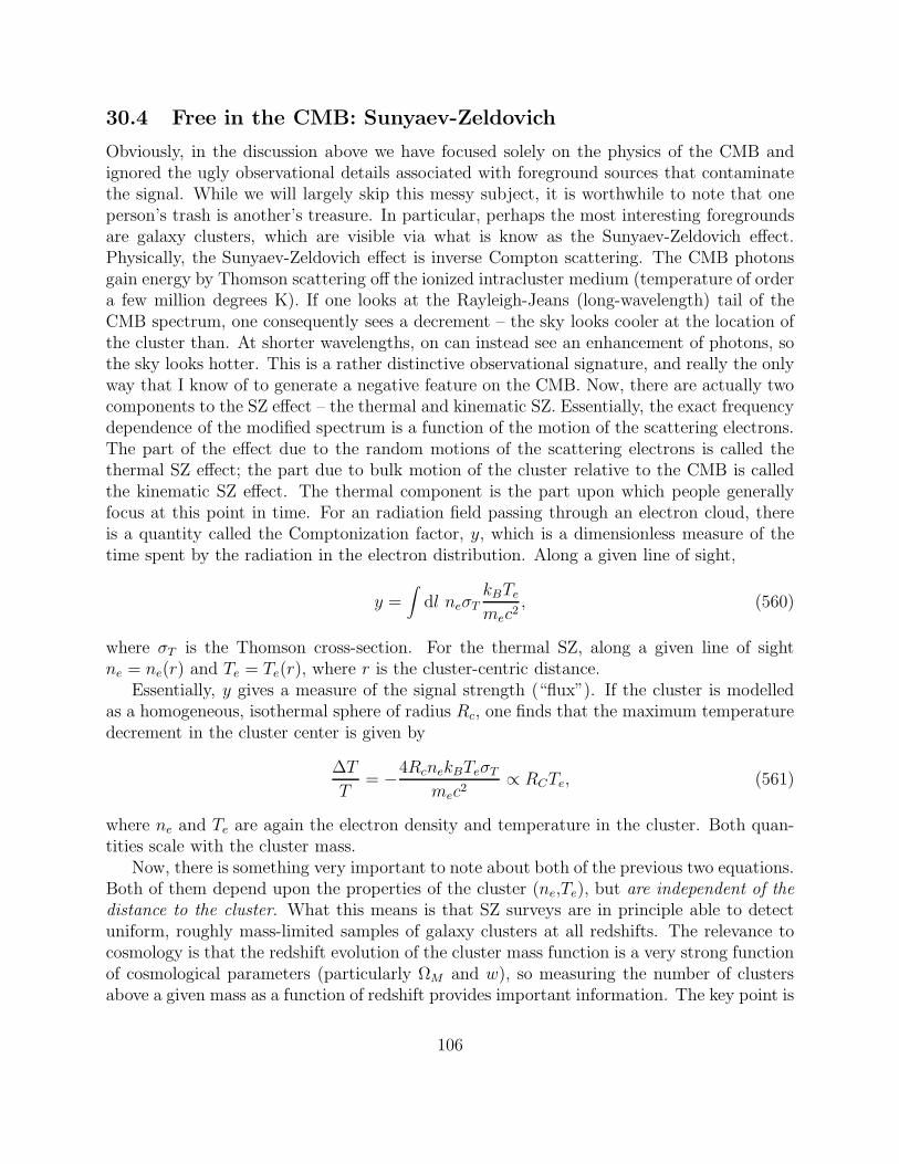
30.4 Free in the CMB: Sunyaev-Zeldovich

Obviously, in the discussion above we have focused solely on the physics of the CMB andignored the ugly observational details associated with foreground sources that contaminatethe signal. While we will largely skip this messy subject, it is worthwhile to note that oneperson’s trash is another’s treasure. In particular, perhaps the most interesting foregroundsare galaxy clusters, which are visible via what is know as the Sunyaev-Zeldovich effect.Physically, the Sunyaev-Zeldovich effect is inverse Compton scattering. The CMB photonsgain energy by Thomson scattering off the ionized intracluster medium (temperature of ordera few million degrees K). If one looks at the Rayleigh-Jeans (long-wavelength) tail of theCMB spectrum, one consequently sees a decrement – the sky looks cooler at the location ofthe cluster than. At shorter wavelengths, on can instead see an enhancement of photons, sothe sky looks hotter. This is a rather distinctive observational signature, and really the onlyway that I know of to generate a negative feature on the CMB. Now, there are actually twocomponents to the SZ effect – the thermal and kinematic SZ. Essentially, the exact frequencydependence of the modified spectrum is a function of the motion of the scattering electrons.The part of the effect due to the random motions of the scattering electrons is called thethermal SZ effect; the part due to bulk motion of the cluster relative to the CMB is calledthe kinematic SZ effect. The thermal component is the part upon which people generallyfocus at this point in time. For an radiation field passing through an electron cloud, thereis a quantity called the Comptonization factor, y, which is a dimensionless measure of thetime spent by the radiation in the electron distribution. Along a given line of sight,

y =∫

dl neσTkBTemec2

, (560)

where σT is the Thomson cross-section. For the thermal SZ, along a given line of sightne = ne(r) and Te = Te(r), where r is the cluster-centric distance.

Essentially, y gives a measure of the signal strength (“flux”). If the cluster is modelledas a homogeneous, isothermal sphere of radius Rc, one finds that the maximum temperaturedecrement in the cluster center is given by

∆T

T= −4RcnekBTeσT

mec2∝ RCTe, (561)

where ne and Te are again the electron density and temperature in the cluster. Both quan-tities scale with the cluster mass.

Now, there is something very important to note about both of the previous two equations.Both of them depend upon the properties of the cluster (ne,Te), but are independent of thedistance to the cluster. What this means is that SZ surveys are in principle able to detectuniform, roughly mass-limited samples of galaxy clusters at all redshifts. The relevance tocosmology is that the redshift evolution of the cluster mass function is a very strong functionof cosmological parameters (particularly ΩM and w), so measuring the number of clustersabove a given mass as a function of redshift provides important information. The key point is

106

that this is an extremely sensitive test. The big stumbling block with cluster mass functionsis systematic rather than statistical – relating observed quantities to mass. A nice aspectof the SZ approach is that they should be roughly mass-limited, although you still want tohave other data (x-ray, optical) to verify this.

Observationally, the SZ folk have be “almost” ready to conduct blind cluster searches forabout a decade (even when I was starting grad school), but it is only in the past year thatclusters have begun to be discovered in this way.

Another application of the SZ effect, which is perhaps less compelling these days, is directmeasurement of the Hubble parameter. This is done by using the ∆T/T relation to get Rc

and then measuring the angular size of the cluster. When done for an ensemble of clustersto minimize the statistical errors, this can be used to obtain H0 (or more generally ΩM andΩΛ if one spans a large redshift baseline). In practice, large systematic uncertainties havelimited the usefulness of this test.

The above is a very quick discussion. If you are particularly interested in the SZ effect,I recommend Birkinshaw astro-ph/9808050.

31 Dark Matter

Time to turn our attention to the dark side of the universe, starting with dark matter. Thegeneral definition of dark matter is any matter from which we cannot observe electromagneticradiation. By this definition, we include such mundane objects as cool white dwarfs as well asmore exotic material. As we shall see though, there is now strong evidence for a componentof exotic, non-baryonic dark matter that dominates the total matter density.

31.1 Classic Observational Evidence

Galaxy ClustersThe first evidence for dark matter was the observation by Fritz Zwicky (1933) that thevelocity dispersion of the Coma cluster is much greater than can be explained by the visiblematter. This is a simple application of standard dynamics, where

GM

r2=v2

r=

2σ2

r. (562)

GM

r= 2σ2 (563)

GL

r

(

M

L

)

= 2σ2 (564)

(

M

L

)

=2σ2r

GL, (565)

where L is the total cluster luminosity and M/L is the mass-to-light ratio. Typical stellarmass to light ratios are of order a few (M⊙/L⊙ = 1; integrated stellar populations M/L <

107

10). If you plug in appropriate numbers for galaxy clusters, you get M/L ∼ 200 [100-500]– a factor of 10-50 higher than the stellar value. This was the first direct evidence that thebulk of matter on cluster scales is in a form other than stars.

In recent years other observations have confirmed that clusters indeed have such largemasses (gravitational lensing, X-ray temperatures), and M/L has been shown to be a func-tion of the halo mass – i.e. lower mass-to-light ratios for smaller systems (see figure in class).Still, this observation was considered little more than a curiosity until complementary ob-servations of galaxy rotation curves in the 1970’s.Rotation CurvesIn the early 1970’s Rubin and Ford compiled the first large sample of galaxy rotation curves,finding that the rotation curves were flat at large radii. In other words, the rotation curvesare consistent with solid-body rather than Keplerian rotation, which argues that the observeddisk is embedded in a more massive halo component. These observations were the ones thatelevated the idea of dark matter from an idle curiosity to a central feature of galaxies thatrequired explanation. Subsequent work also showed that the presence of a massive halo isactually required in galactic dynamics to maintain disk stability, and the above data playeda key role in influencing the later development of the cold dark matter model of structureformation (Blumenthal et al. 1984).

31.2 Alternatives

Is there any way to avoid the consequence of dark matter? The most popular alternative isto modify gravity at large distances. One of the more well-known of these theories is calledModified Newtonian Dynamics (MOND, Milgrom 1980). The idea here is to change theNewtonian force law at small accelerations from F = ma to F = µma, where µ = 1 if a > a0

and µ = a/a0 if a < a0. In our normal everyday experience, we experience a > a0, so themodification to the acceleration would only matter for very small accelerations. Now, if weconsider the gravitational attraction of two objects,

F =GMm

r2= µma. (566)

If we assume that at large distances a < a0 so that µ = a/a0, then

GM

r2=a2

a0

(567)

a =

√GMa0

r. (568)

For a circular orbit,

a =v2

r=

√GMa0

r, (569)

sov = (GMa0)

1/4 (570)

108

As you can see, this yields a circular velocity that is constant with radius – a flat rotationcurve. One can calculate the required constant for the galaxy, finding a0 ≃ 10−10 m s−2.Similar arguments can be made for explaining the cluster velocity dispersions.

A limitation of MOND is that, like Newtonian gravity, it is not Lorentz covariant. Con-sequently, just as GR is required as a foundation for cosmology, one would need a Lorentzcovariant version of the theory to test it in a cosmological context. There is now one suchLorentz covariant version, TeVeS (Tensor-Vector-Scalar theory; Bekenstein 2004), from whichone can construct cosmological world models. However, in order to provide a viable alterna-tive to dark matter, TeVeS – or any other modified gravity theory – must be as successfulas dark matter in explaining a large range of modern cosmological observations, includingour entire picture of structure formation from initial density fluctuations.

31.3 Modern Evidence for Dark Matter

So why do we believe that dark matter exists? While modified gravity is an interestingmeans of attempting to avoid the presence of dark matter, at this point I would argue thatwe have a preponderance of evidence against this hypothesis. One relatively clean exampleis the Bullet Cluster. For this system, we (Clowe et al. 2004,2006) used weak lensing todemonstrate that the mass and intracluster gas (which contains the bulk of the baryons)are offset from one another due to viscous drag on the gas. Hence the baryons cannot beresponsible for the lensing and there must be some other component causing the lensing.The TeVeS community has attempted to reconcile this observation with modified gravity,but are unable to do so using baryons alone. The are able to manage rough qualitative (andI would argue poor) agreement if they assume that 80% of the total matter density is in2 eV neutrinos. [It is worth noting that 2 eV is the maximum mass that a neutrino canhave if one relies on constraints that are independent of GR, but new experiments should berunning in the next few years that will significantly lower this mass limit.] Thus, even withmodified gravity one still requires 80% of the total matter density to be ‘dark’.

Aside from this direct evidence, a compelling argument can be made based upon theremarkable success of the cold dark matter model in explaining the growth and evolution ofstructure in the Universe. Dark matter provides a means for seed density fluctuations to growprior to the surface of last scattering, and CDM reproduces the observed growth of structurein the Universe from the CMB to z = 0. It is not obvious a priori that this should be thecase. As we have seen, the cosmic microwave background provides us with a measurementof the ratio between total and baryonic matter, arguing that there is roughly a factor of 7more matter than the baryon density, and yields a measurement of the total matter density(assuming GR is valid). These results from the CMB, with the baryon density confirmedby Li abundance measurements, yield densities that, when used as inputs to CDM, producethe observed structures at the present. The fact that the bulk of the total matter is darkmatter seems unavoidable.

109

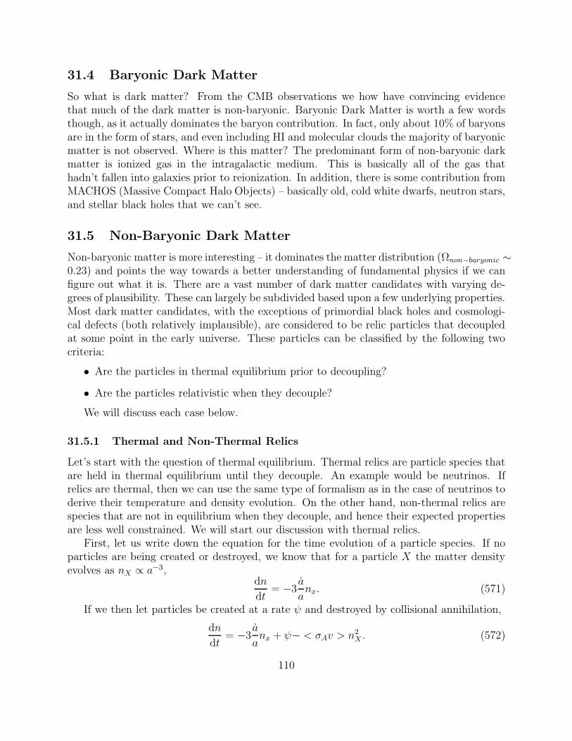
31.4 Baryonic Dark Matter

So what is dark matter? From the CMB observations we how have convincing evidencethat much of the dark matter is non-baryonic. Baryonic Dark Matter is worth a few wordsthough, as it actually dominates the baryon contribution. In fact, only about 10% of baryonsare in the form of stars, and even including HI and molecular clouds the majority of baryonicmatter is not observed. Where is this matter? The predominant form of non-baryonic darkmatter is ionized gas in the intragalactic medium. This is basically all of the gas thathadn’t fallen into galaxies prior to reionization. In addition, there is some contribution fromMACHOS (Massive Compact Halo Objects) – basically old, cold white dwarfs, neutron stars,and stellar black holes that we can’t see.

31.5 Non-Baryonic Dark Matter

Non-baryonic matter is more interesting – it dominates the matter distribution (Ωnon−baryonic ∼0.23) and points the way towards a better understanding of fundamental physics if we canfigure out what it is. There are a vast number of dark matter candidates with varying de-grees of plausibility. These can largely be subdivided based upon a few underlying properties.Most dark matter candidates, with the exceptions of primordial black holes and cosmologi-cal defects (both relatively implausible), are considered to be relic particles that decoupledat some point in the early universe. These particles can be classified by the following twocriteria:

• Are the particles in thermal equilibrium prior to decoupling?

• Are the particles relativistic when they decouple?

We will discuss each case below.

31.5.1 Thermal and Non-Thermal Relics

Let’s start with the question of thermal equilibrium. Thermal relics are particle species thatare held in thermal equilibrium until they decouple. An example would be neutrinos. Ifrelics are thermal, then we can use the same type of formalism as in the case of neutrinos toderive their temperature and density evolution. On the other hand, non-thermal relics arespecies that are not in equilibrium when they decouple, and hence their expected propertiesare less well constrained. We will start our discussion with thermal relics.

First, let us write down the equation for the time evolution of a particle species. If noparticles are being created or destroyed, we know that for a particle X the matter densityevolves as nX ∝ a−3,

dn

dt= −3

a

anx. (571)

If we then let particles be created at a rate ψ and destroyed by collisional annihilation,

dn

dt= −3

a

anx + ψ− < σAv > n2

X . (572)

110

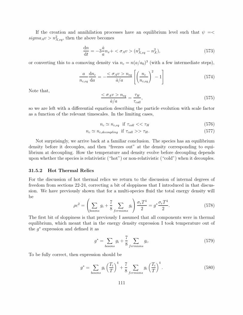
If the creation and annihilation processes have an equilibrium level such that ψ =<sigmaAv > n2

X,eq, then the above becomes

dn

dt= −3

a

anx+ < σAv > (n2

X,eq − n2X), (573)

or converting this to a comoving density via nc = n(a/a0)3 (with a few intermediate steps),

a

nc,eq

dncda

= −< σAv > neqa/a

(

ncnc,eq

)2

− 1

(574)

Note that,< σAv > neq

a/a=

τHτcoll

, (575)

so we are left with a differential equation describing the particle evolution with scale factoras a function of the relevant timescales. In the limiting cases,

nc ≃ nc,eq if τcoll << τH (576)

nc ≃ nc,decoupling if τcoll >> τH . (577)

Not surprisingly, we arrive back at a familiar conclusion. The species has an equilibriumdensity before it decouples, and then “freezes out” at the density corresponding to equi-librium at decoupling. How the temperature and density evolve before decoupling dependsupon whether the species is relativistic (“hot”) or non-relativistic (“cold”) when it decouples.

31.5.2 Hot Thermal Relics

For the discussion of hot thermal relics we return to the discussion of internal degrees offreedom from sections 22-24, correcting a bit of sloppiness that I introduced in that discus-sion. We have previously shown that for a multi-species fluid the total energy density willbe

ρc2 =

∑

bosons

gi +7

8

∑

fermions

gi

σrT4

2= g∗

σrT4

2. (578)

The first bit of sloppiness is that previously I assumed that all components were in thermalequilibrium, which meant that in the energy density expression I took temperature out ofthe g∗ expression and defined it as

g∗ =∑

bosons

gi +7

8

∑

fermions

gi. (579)

To be fully correct, then expression should be

g∗ =∑

bosons

gi

(

TiT

)4

+7

8

∑

fermions

gi

(

TiT

)4

. (580)

111

We also learned that the entropy for the relativistic components is

sr =2

3g∗SσrT

3. (581)

The second bit of sloppiness is that in the previous discussion I treated g∗ and g∗S inter-changeably, which is valid for most of the history of the universe, but not at late times (likethe present). The definition of g∗S is

g∗S =∑

bosons

gi

(

TiT

)3

+7

8

∑

fermions

gi

(

TiT

)3

. (582)

Now, for a species that is relativistic when it decouples (3kT >> mc2), entropy conser-vation requires that

g∗S,XT30X = g∗S0T

30γ , (583)

where

g∗S0 = 2 +7

8× 2×Nν ×

(

T0ν

T0γ

)3

≃ 3.9 (584)

for Nν = 3.Anyway, you can also calculate the number density in the same way as before,

nX = αgXζ(3)

π2

(

kBTXhc

)3

(585)

n0X

n0γ

= αgX2

(

T0X

T0r

)3

(586)

n0X = n0γαgS,X2

g∗S,Xg∗S,0

, (587)

where α = 3/4 or α = 1 depending on whether the particle is a fermion or boson. Thedensity parameter in this case is

ΩX =mXn0X

ρ0c≃ 2αgX

(

g∗S,Xg∗S,0

)

(

mX

102 eVh−2

)

(588)

31.5.3 Cold Thermal Relics

The situation is not as straightforward for non-relativistic (“cold”) thermal relics. In thiscase, at decoupling the number density is described by the Boltzmann distribution,

ndecoupling,X =gXh

(

mXkBT

2π

)3/2

exp

(

−mxc2

kBT

)

(589)

112

and hence the present day density is lower by a factor of a3,

n0X = ndecoupling,Xg∗S,0g∗X

(

T0r

Tdecoupling

)3

. (590)

The catch is figuring out what the decoupling temperature is. As usual, you set τH = τcoll.We previously saw that

τH ≃(

3

32πGρ

)1/2

≃ 0.3hTP√g∗SkBT

2, (591)

(as in equation 7.1.9 in your book), and that

τcoll = (nσv)−1 . (592)

The definition of the σv part is a bit more complex, since the cross-section can be velocitydependent. If we parameterize σv as

< σv >= σ0

(

kBT

mXc2

)q

, (593)

with q normally having a value of 0 or 1 (i.e. σ ∝ v−1 or σ ∝ v, then working through thealgebra one would find that

ρ0X ≃ 10√

g∗X(kBT0r)

3

hc4σ0mP

(

mXc2

kBTdecoupling

)q+1

(594)

31.5.4 Significance of Hot versus Cold Relics

Physically, there is a much more significant difference between hot and cold relics that howto calculate the density and temperature. The details of the calculations we will have toleave for another course (they depend upon Jeans mass calculations, which are covered inchapter 10). The basic concept though is that after relativistic particles decouple from theradiation field, they are able to “free-stream” away from the locations of the initial densityperturbations that exist prior to recombination. In essence, the velocity of the particles isgreater than the escape velocity for the density fluctuations that eventually lead to galaxy andgalaxy cluster formation. The net effect is damp the amplitude of these density fluctuations,which leads to significantly less substructure than is observed on small scales.

In contrast, cold relics (cold dark matter) only damp out structure on scales much smallerthan galaxies, so the fluctuations grow uninterrupted. The difference in the two scenariosis rather dramatic, and we can easily exclude hot dark matter as a dominant constituent.Finally, our observations of local structures also tells us that the dark matter must currentlybe non-relativistic or else it would not remain bound to galaxies.

113

31.5.5 Non-Thermal Relics

We have shown how one would calculate the density of particles for relics that were inequilibrium when they decoupled. There does however exist the possibility that the darkmatter consists of particles that were not in thermal equilibrium. If this is the case, then weare left is a bit of a predicament in this regard, as there is no a priori way to calculate thedensity analogous to the previous sections. As we shall see, one of the leading candidatesfor dark matter is a non-thermal relic.

31.6 Dark Matter Candidates

At this point we have argued that the dark matter must be non-baryonic and “cold”, but notnecessarily thermal. While the preferred ideas are that dark matter is a particle relic, thereare non-particle candidates as well. Right now we will briefly review a few of the leadingparticle candidates, which are motivated by both cosmology and particle physics.

31.6.1 Thermal Relics: WIMPS

Weakly interacting massive particles (WIMPS) are a favorite dark matter candidates. Thisclass of particles are cold thermal relics. We worked out above a detailed expression for ρ0X ,but to first order we can make the approximation that,

ΩWIMP ≃10−26 cm3 s−1

< σv >. (595)

For ΩDM ∼ 1 (0.3 being close enough), the annihilation cross section < σv > turns out tobe about what would be predicted for particles with electroweak scale interactions – hence“weakly interacting” in the name.

From a theoretical perspective, this scale of the annihilation cross-section is potentially avery exciting clue to both the nature of dark matter and new fundamental physics – specif-ically the idea of super-symmetry. Stepping back for a moment, the notion of antiparticles(perhaps rather mundane these days) comes from Dirac (1930), who predicted the existenceof positrons based upon theoretical calculations that indicated electrons should have a sym-metric antiparticle. It is now a fundamental element of particle physics that all particleshave associated, oppositely charged antiparticles.

What is relatively new is the idea of “super-symmetry”. Super-symmetry (SUSY) is ageneralization of quantum field theory in which bosons can transform into fermions and viceversa. In a nutshell, the idea of super-symmetry is that every particle (and antiparticle)has a super-symmetric partner with opposite spin statistics (spin different by 1/2). In otherwords, every boson has a super-symmetric partner that is a fermion, and every fermion hasa super-symmetric partner that is a boson. The partners for quarks and leptons are calledsquarks and sleptons; parters for photons are photinos, and for neutral particles (Higgs, etc)are called neutralinos.

114

Now why would one want to double the number of particles? First, SUSY provides aframework for potential unification of particle physics and gravity. Of the numerous attemptsto make general relativity consistent with quantum field theory (unifying gravity with thestrong and electroweak forces), all of the most successful attempts have required a newsymmetry. In fact, it has been shown (the Coleman-Mandual theorum) that there is no wayto unify gravity with the standard gauge theories that describe the strong and electroweakinteractions without incorporating some supersymmetry.

There are also several other problems that SUSY addresses – the mass hierarchy problem,coupling constant unification, and the anomalous muon magnetic moment. We won’t go intothese here, other than to point out that they exist, and briefly explain the coupling constantproblem. Essentially, the strength of the strong, weak, and electromagnetic forces is set bythe coupling constants (like αwk, which the book calls gwk). These coupling “constants”(similar to the Hubble constant) are actually not constant, but dependent upon the energyof the interactions. It was realized several decades ago that the coupling constants for thethree forces should approach the same value at 1015 GeV, allowing “grand unification” ofthe three forces. In recent years though, improved observations of the coupling constantshave demonstrated in that in the Standard Model the three coupling constants in fact neverapproach the same value. Supersymmetry provides a solution to this problem – if super-symmetric particles exist and have appropriate masses, they can modify the above pictureand force the coupling constants to unify.

The way in which this ties back into dark matter is that the neutral charge super-symmetric particles (broadly grouped under the name neutralinos) become candidate darkmatter particles. Due to a broken symmetry in supersymmetry, the super-symmetric partnerparticles do not have the same masses as normal particles, and so can potentially be the darkmatter.

There are many flavors of sypersymmetry, but one popular (and relatively simple) versioncalled the Minimal Super-symmetric Standard Model (MSSM) illustrates the basic idea. InMSSM, one takes the standard model, and adds the corresponding super-symmetric partners(plus an extra Higgs doublet). The lightest super-symmetric particle (LSP) is stable (i.edoesn’t decay – an obvious key property for dark matter), and typically presumed to be themain constituent of dark matter in this picture. The combined requirements that the SUSYmodel both unify the forces and reproduce the dark matter abundance gives interestingconstraints on the regime of parameter space in which one wants to search. A somewhatold, but illustrative, example is de Boer et al. (1996). These authors find that there aretwo regions of parameter space where the constraints can be simultaneously satisfied. Inthe first, the mass of the Higgs particle is relatively light (mH < 110 GeV) and the LSPabundance is ΩLSPh

2 = 0.42 with mLSP = 80 GeV. In the other region, mH = 110 GeV andthe abundance is ΩLSPh

2 = 0.19. These values clearly bracket the current best observationaldata. Incidentally, note that all of these particles are very non-relativistic at the GUT scale(1015 GeV), and so quite cold.

115

31.6.2 Axions

Axions are the favorite among the non-thermal relic candidates, and like WIMPS are popularfor reasons pertaining to particle physics as much as cosmology. The axion was originallyproposed as part of a solution to explain the lack of CP (charge-parity) violation in strongnuclear interactions – e.g. quarks and gluons, which are the fundamental constituents of pro-tons and neutrons (see http://www.phys.washington.edu/groups/admx/the axion.html andhttp://www.llnl.gov/str/JanFeb04/Rosenberg.html for a bit of background). CP is violatedfor electroweak interactions, and in the standard model it is difficult to explain why thestrong interaction should be finely-tuned to not violated CP in a similar fashion. Somewhatanalogous to the case of supersymmetry, a new symmetry (Peccei-Quinn symmetry) hasbeen proposed to explain this lack of CP violation. A nice aspect of this solution is that itexplains why neutrons don’t have an electrical dipole moment (although we won’t discussthis).

An important prediction of this solution is the existence of a particle called the axion.Axions have no electric charge or spin and interact only weakly with normal matter – exactlythe properties one requires for a dark matter candidate. There are two very interestingdifferences between axions and WIMPS though. First, axions are very light. Astrophysicaland cosmological constraints require that 10−6 < maxion < 10−3 eV – comparable to theplausible mass range for neutrinos. Specifically, the requirement m < 10−3 eV is based uponSN 1987a – if the axion mass were larger than this value, then the supernova core shouldhave cooled by both axion and neutrino emission (remember, they’re weakly interacting, butcan interact) and the observed neutrino burst should have been much shorter than observed.The lower bound, somewhat contrary to intuition, comes from the requirement that thetotal axion density not exceed the observed dark matter density. Axions lighter than 10−6

eV would have been overproduced in the Big Bang, yielding Ω >> ΩM .At a glance, one might think that the low mass of the axion would be a strong argument

against axions being dark matter. After all, shouldn’t axions be relativistic if they are solight? The answer would be yes – if they were thermal relics. Axions are never coupled tothe radiation field though, and the mechanism that produces them gives them very littleinitial momentum, so axions are in fact expected to be quite cold relics.

31.7 Other Candidates

The above two sections describe what are believed to be the most probable dark mattercandidates. It should be pointed out though that (1) WIMPS are a broad class and thereare many options within this category, and (2) there are numerous other suggestions fordark matter. These other suggestions include such exotic things as primordial black holesformed at very early times/high density, and cosmic strings. While I would suspect thatthese are rather unlikely, they cannot be ruled out. Similarly, it remains possible that allof the above explanations are wrong. Fortunately, there are a number of experiments nowunderway that should either detect or eliminate some of these candidates. To go out ona limb, my personal guess is that things will turn out to be somewhat more complicated

116

than expected. Specifically, it seems plausible that both axions and WIMPS exist and eachcontribute at some level to the total matter density.

31.8 Detection Experiments

So how might one go about detection dark matter? Given the wide range of masses andinteraction cross-sections for the various proposed candidates, the first step is basically this– pick what you believe is the most plausible candidate and hope that you are correct. Ifyou are, and can be the first to find it, then a Nobel prize awaits. Conversely, if you pickthe wrong candidate you could very well spend much of your professional career chasing aghost. Assuming that you are going to search though, let’s take a look at how people areattempting to detect the different particles.

Something to keep in mind in general in this discussion is that there are essentially twoclasses of dark matter searches – terrestrial direct detection experiments and astrophysicalindirect detection observations. Keep this in mind.

117

32 An Aside on Scalar Fields

In the discussion of inflation we talked about inflation being driven by the vacuum energy ina scalar field. Since there is some confusion on the concept of scalar fields, let us revisit thismatter briefly. Mathematically, a scalar field is simply a field that at each point in spacecan be represented by a scalar value. Everyday examples include things like temperature ordensity.

Turning more directly to physics, consider gravitational and electric fields. In Newtoniangravity, the gravitational potential is a scalar field Φ defined by Poisson’s equation,

∇2Φ = −4πGρ, where

F = −∇Φ, and

V (Φ) =∫

ρ(x)Φ(x)d3x.

Similarly, for an electric potential φ,

∇2φ = −4πGρ, where

E = −∇φ, and

V (φ) =∫

ρφd3x.

In particle physics (quantum field theory), scalar fields are associated with particles. Forinstance the Higgs field is associated with the predicted Higgs particle. The Higgs field isexpected to have a non-zero value everywhere and be responsible for giving all particles mass.

In the context of inflation we are simply introducing a new field that follows the samemathematical formalism. The term vacuum energy density simply means that a region ofvacuum that is devoid of matter and radiation (i.e. no gravitational or electromagneticfields) has a non-zero energy density due to energy contained in a field such as the inflatonfield (named because in the particle physics context it should be associated with an inflatonparticle). During inflation this energy is liberated from the inflaton field. Note that darkenergy does not have to be vacuum energy though.

33 Dark Energy

33.1 Generic Properties

As we have seen during the semester, the observable Friedmann equation is H = H0E(z),where

E(z) =

[

∑

i

Ω0i(1 + z)3(1+wi) + (1−∑

i

Ω0i)(1 + z)2

]1/2

, (596)

and the energy density of any component goes at

ρ = ρ0(1 + z)3(1+w), (597)

118

where w is the equation of state. Recall that w = 0 for dust-like matter, w = 1/3 forradiation, and w = −1 for a cosmological constant. While we have previously discussedthe possibility of dark energy corresponding to a cosmological constant, this is not the onlypossibility. Indeed, the most generic definition is that any substance or field that has anequation of state with w < −1/3, which corresponds to a negative energy density, is darkenergy. Perhaps the single most popular question in cosmology at present is the nature ofdark energy, and the best means of probing this question is by attempting to measure w(z).

33.2 Fine Tuning Problem

Let us start by framing this question. As you may have noticed, a recurring theme incosmology is the presence of what are called “fine-tuning” problems. These tend to be themost severe problems and the ones that point the way to new physics (like inflation). Inthe current context, there is a very significant fine-tuning problem associated with either acosmological constant or a dark energy component with a constant equation of state. Forthe specific case of the cosmological constant, the current concordance model values implythat the universe only started accelerating at z ≃ 0.7 and that the cosmological constantonly began to dominate at z ≃ 0.4. The question is why we should be so close in time to theera when the dark energy begins to dominate – a point where we can see evidence for theacceleration, but haven’t yet had structures significantly accelerated away from one another.Put another way, to get the current ratio of ρΛ/ρm ≈ 2, we require that at the Planck timeρΛ/ρr ≈ 10−120. This issue is intricately related to the phrasing of the cosmological constantproblem that we discussed earlier this semester, albeit in a somewhat more general form.What, then, are possibilities for dark energy, and can these possibilities also alleviate thisfine-tuning problem?

33.3 Cosmological Constant

The cosmological constant remains the leading candidate for dark energy, as recent observa-tions strongly argue that at z = 0 we have w = −1 to within 10%. If it is truly a cosmologicalconstant, then avoiding the fine tuning problem will require either new physics or a novelsolution (like inflation as a solution to other fine tuning problems).

33.4 Quintessence and Time Variation of the Equation of State

Quintessence is the general name given to models with w ≥ −1. Quintessence modelswere introduced as alternatives to the cosmological constant for two reasons – (1) becauseyou can. If we don’t know why there should be a cosmological constant, why not proposesomething else, and (2) because if the equation of state is made to be time-dependent, onecan potentially avoid the fine-tuning problem described above.

There are many types of quintessence, but one feature that most have in common is that,like a cosmological constant, they are interpreted as being associated with the energy density

119

of scalar fields. These are generally taken to have

ρ =1

2φ2 + V (φ) (598)

p =1

2φ2 − V (φ) (599)

Note that in order to generate an accelerated expansion, the above relations require that

φ2 < V (φ) if w < −1

3(600)

φ2 <2

3V (φ) if w < −1

2, (601)

which is equivalent to saying that the potential term dominates over the kinetic term – notnecessarily quite slow roll, but not too far off. As you go to w = −1, you very much moveinto the slow roll regime.

One particularly entertaining class of quintessence models correspond to what are called“tracker” models, in which the energy density of the scalar field remains close to the mat-ter/radiation density through most of the history of the universe. It turns out that if thepotential is sufficiently steep that

V ′′V

(V ′)2> 1, (602)

the scalar field rolling down the potential approaches a common evolutionary path such thatthe dark energy tracks the radiation energy density as desired.

33.5 Time Variation of the Equation of State

Now, as this will be part of the discussion as we proceed, there is one important distinctionto note if we have a time variable equation of state. The standard equation

H2 = H20

[

Ωw(1 + z)3(1+w)]

(603)

only holds for a constant value of w. If w is also a function of redshift, then it must also beintegrated appropriately, and what you end up with is

H2 = H20

[

Ωw exp

(

3∫ ln(1+z)

0(1 + w(x))d ln(1 + x).

)]

(604)

The origin of this expression can be seen by returning to the derivation of ρ(z) in §10,where we derived that for a constant w

ρ = ρ0(1 + z)3(1+w), (605)

given an adiabatic expansion. If we start with the intermediate equation from that derivation,

dρ

ρ= − (1 + w)

da3

a3(606)

120

we see that for a variable w

dρ

ρ= −(1 + w(a))d ln a3 (607)

dρ

ρ= −(1 + w(z))d ln(1 + z)3 (608)

ln

(

ρ

ρ0

)

= 3∫ ln(1+z)

0(1 + w(z))d ln(1 + z) (609)

ρ

ρ0= exp

(

3∫ ln(1+z)

0(1 + w(z))d ln(1 + z)

)

(610)

(611)

In principle, you can insert any function of w(z) that you prefer. At the moment though,the data isn’t good enough to constrain a general function, so people typically use a firstorder parameterization along the lines of

w = w0 + w1z

1 + z. (612)

33.6 Phantom Energy

The recent observations have given rise to serious consideration of one of the more bizarrepossibilities – w < −1. Knop et al. (2003) actually showed that if you removed the priors onΩm for the data existing at the time, then the dark energy equation of state yielded a 99%probability of having w < −1. Current data have improved, with uncertainties somewhatmore symmetric about w = −1, but this possibility persists.

Models with w < −1 violate what is know as the weak energy condition, which simplymeans that for these models ρc2 + p < 0 – the universe has a net negative energy density.If the weak energy condition is violated and the equation of state is constant, this leads tosome rather untenable conclusions, such as.

(1) The scale factor becomes infinite in a finite time after the phantom energy begins todominate. Specifically, if w < 1

a ≃ aeq

[

(1 + w)t

teq− w

]2/3(1+w)

, (613)

where the subscript eq denotes the time when the matter and phantom energy densities areequal. Note that the exponent in this equation is negative, which means that the solution issingular (a→∞) at a finite point in the future when

t = teqw

1 + w. (614)

For example, for w = −1.1, this says that the scale factor diverges when t = 10teq (so we’reover a tenth of the way there!). If we look back at the standard equation for the Hubble

121

parameter, we see that it also diverges (which is consistent), as does the phantom density,which increases as

ρ ∝[

(1 + z)t

teq− w

]−2

. (615)

The above divergences have been termed the “Big Rip”.(2) The sound speed in the medium, v = (|dp/dρ|)1/2 can exceed the speed of light.It is important to keep in mind that the above issues only transpire if the value of w is

constant. You can get away with temporarily having w < −1.

33.7 Chaplygin Gas

The Chaplygin gas is yet another way to get a dark energy equation of state. Assume thatthere is some fluid which exerts a negative pressure of the form

p =−Aρ. (616)

For an adiabatic expansion, where dE = −pdV , or d(ρa3) = −pda3, this yields

ρ = (A+Ba−6)1/2 = (A+B(1 + z)6)1/2.(see below) (617)

If you look at the limits of this equation, you see that as z →∞,

ρ→ B1/2(1 + z)3, (618)

which is the standard density equation for pressureless dust models, while at late times,

ρ→ A1/2 = constant, (619)

similar to a cosmological constant.The nice aspect of this solution is that you have a simple transition between matter and

dark energy dominated regimes. In practice, there are certain problems with the Chaplygingas models though (such as structure formation). The more recent revision to this proposalhas been for what is called a “generalized Chaplygin gas”, where

p ∝ −ρ−α, (620)

which gives and equation of state

w(z) = − |w0||w0|+ (1− |w0|)(1 + z)3(1+α)

, (621)

where w0 is the current value of the equation of state. Note that we are now seeing anotherexample of a time-dependent equation of state.

122

Derivation of equation for density - starting from the adiabatic expression,

ρda3 + a3dρ =A

ρda3 (622)

a3ρdρ = −(ρ2 − A)da3 (623)

ρdρ

ρ2 − A =−da3

a3(624)

1/2 ln(ρ2 − A) = B ln a−3 (625)

(ρ2 − A) = Ba−6 (626)

ρ = (A+Ba−6)1/2 (627)

33.8 Cardassian Model

Yet another approach to the entire problem is to modify the Friedmann equation, as withthe Randall-Sundrum model at early times, replacing

H2 =8πG

3ρ (628)

with a general form of H2 = g(ρ), where g is some arbitrary function of only the matter andradiation density. The key aspect of Cardassian models is that they don’t include a vacuumcomponent or curvature – the “dark energy” is entirely contained in this modification of theFriedmann equation.

A simple version of these models is

H2 =8πG

3ρ+Bρn, where n < 2/3. (629)

In Cardassian models the additional term is negligible at early times and only begins todominate recently. Once this term dominates, then a ∝ t2/(3n). The key point though isthat for these models the universe can be flat, matter-dominated, and accelerating with asub-critical matter density.

Moving beyond the above simple example, the “generalized Cardassian model” has

H2 =8πG

3ρ

1 +

(

ρ

ρcard

)q(n−1)

1/q

, (630)

where n < 2/3, q > 0 and ρcard is a critical density such that the modifications only matterwhen ρ < ρcard.

Note that in many ways this is eerily reminiscent of MOND. This scenario cannot beruled out though given the current observations, and there is a somewhat better motivationthan in the case of MOND. In particular, modified Friedmann equations arise generically intheories with extra dimensions (Chung & Freese 1999), such as braneworld scenarios.

123

33.9 Other Alternatives

In the brief amount of time that we have in the semester I can only scratch the surface(partially because there are a huge number of theories that are only modestly constrained bythe data). For completeness, I will simply list some of the other proposed solutions to darkenergy, such that you know the names if you wish to learn more. These include k−essence,scalar-tensor models, Quasi-Steady State Cosmology, and Brane world models.

124

34 Gravitational Lensing

Reading: Chapter 19, Coles & LucchinLike many other sections of this course, the topic of gravitational lensing could cover an

entire semester. Here we will aim for a shallow, broad overview. I also note that this sectionof the notes is currently more sparse than the other sections thus far and most of the lecturewas not directly from these notes. For more in depth reading, I refer you to the followingexcellent text on the subject: Gravitational Lensing: Strong, Weak & Micro, Saas-FeeAdvanced Course 33, Meylan et al. (2005).

34.1 Einstein GR vs. Newtonian

A pseudo-Newtonian derivation for the deflection of light yields

α =2GM

rc2. (631)

In general relativity however there is an extra factor of 2 such that the deflection is

α =4GM

rc2. (632)

This can be derived directly from the GR spacetime metric for the weak field limit arounda mass M ,

ds2 =(

1 +2GM

rc2

)

c2dt2 −(

1− 2GM

rc2

)

dl2, (633)

as you will do in your homework.-refer to book discussion of deflection of light by the sun.

34.2 Gravitational Optics

I refer the reader here to the Figure 19.1 in Coles & Lucchin or Figure 12 in the Saas-Feetext. If one considers a beam of light passing through a gravitational field, the amount bywhich the beam is deflected is determined by the gradient of the potential perpendicular tothe direction of the beam. Physically, a gradient parallel to the path clearly can have noeffect, and the stronger the gradient the more the light is deflected. The deflection angle isdefined as

α =2

c2

∫

∇⊥Φdl, (634)

where l is the direction of the beam. The above is formally only valid in the limit that thedeflection angle is small (i.e. weak field), which for a point source lens is equivalent to sayingthat the impact parameter ξ is much larger than the Schwarzschild radius (rs ≡ 2GM/cv2).

Definitions: The lens plane is considered to be the plane that lies at the distance of thelens; the source plane is equivalently the plane that lies at the distance of the source. It is

125

common to talk about the locations of objects in the source plane and the image in the lensplane.

A Point Source Lens - For a point source the gravitational potential is

Φ(ξ, x) = − GM

(ξ2 + x2)1/2, (635)

where x is the distance from the lens parallel to the direction of the light ray. Taking thederivative and integrating along dx, one finds

α =2

c2

∫

∇⊥Φdx =4GM

c2ξ, (636)

which is the GR deflection angle that we saw before.Extended Lenses - Now, let us consider the more general case of a mass distribution rather

than a point source. We will make what is called the thin lens approximation that all thematter lies in a thin sheet. In this case, the surface mass density is

Σ(ξ) =∫

ρ(ξ, x)dx, (637)

the mass within a radius ξ is

M(ξ) = 2π∫ ξ

0Σ(ξ′)ξ′dξ′, (638)

and the deflection angle is

α =4G

c2

∫ (ξ − ξ′)Σ(ξ′)

|ξ − ξ′|2 d2ξ′ =4GM

c2ξ, (639)

Another way to think of this is as the continuum limit of the sum of the deflection angles fora distribution of N point masses. Note that in the above equation α is now a two-dimensionalvector.

The Lens equation - Now, look at the figure referenced above. In this figure α, calledthe reduced deflection angle, is the angle in the observers frame between the observed sourceand where the unlensed source would be. The angle β is the angle between the lens and thelocation of the unlensed source. It is immediately apparent that θ, the angle between thelense and the observed source is related to these two quantities by the lens equation,

β = θ − α(θ). (640)

Now, if one assumes that the distances (Ds, Dds,Dd) are large, as will always be the case,then one can immediately show via Euclidean geometry that

α =Dds

Dsα. (641)

126

[Note that equation 19.2.10 in Coles & Lucchin is incorrect – the minus sign should be aplus sign.]

Note that if there is more than one solution to the lens equation then a source at β willproduce several images at different locations.

If we take the definition of α and rewrite the expression in angular rather than spatialcoordinates (ξ = Ddθ), then

α(θ) =Dds

Dsα =

1

πintd2θ′κ(θ′)

θ − θ′|θ − θ′|2 , (642)

where

κ(θ) =Σ(Ddθ)

Σcr(643)

and

Σcr =c2

4πG

Ds

DdDds

. (644)

In the above equations κ is the convergence, and is also sometimes called the dimensionlesssurface mass density. It is the ratio of the surface mass density to the critical surface massdensity Σcr. The significance of Σcr is that for Σ ≥ Σcr the lens is capable of producingmultiple images of sources (assuming that the sources are in the correct locations). This isthe definition of strong lensing, so Σcr is the dividing line between strong and weak lensing.Your book also provides another way of interpreting the critical density, which is that for thecritical density one can obtain β = 0 for any angle theta – i.e. for a source directly behindthe lens all light rays are focused at a well-defined focal length (which of course will differdepending on the angle theta).

Axisymmetric Lenses – Now, let’s consider the case of a circularly symmetric lens. Inthis case,

α(θ) =Dds

Dsα =

Dds

DdDs

4GM(θ)

c2θ=

4GM(θ)

Dc2θ, (645)

where

D ≡ DdDs

Dds

, (646)

and

β = θ − 4GM(θ)

Dc2θ. (647)

The case β = 0 corresponds to

θE =

(

4GM(θE)

Dc2

)1/2

, (648)

where θE is called the Einstein radius. A source at β=0 is lensed into a ring of radius θE .Note that this angle is again simply the deflection angle in GR. One can rewrite the lensingequation in this case for a circularly symmetric lense to be

β = θ − θ2E/θ, (649)

127

or

θ± =1

2

(

β ± (β2 + 4θ2E))

(650)

These solutions correspond to two images – one on each side of the source. One of these isalways at θ < θE , while the other is at θ > θE . In the case of β = 0, the two solutions areobviously both at the Einstein radius.

General Case – Consider the more general case of a lense that lacks any special symmetry.Let us define what is called the deflection potential

ψ(θ) =2

Dc2

∫

Φ(Ddθ, x)dx. (651)

The gradient of this deflection potential with respect to theta is

∇θψ = Dd∇ξψ =Dds

Ddα = α (652)

and the Laplacian is∇2θψ = 2κ(θ) = 2Σ/Σcr. (653)

The significance of this is that we can express the potential and deflection angle in terms ofthe convergence,

ψ(θ) =1

π

∫

κ(θ) log |θ − θ′|d2θ′ (654)

α(θ) =1

π

∫

κ(θ)θ − θ′|θ − θ′|2d2θ′ (655)

(skip the last two equations in class).We will momentarily see why Φ(θ) is a useful quantity. Let us return to the lensing

equationβ = θ − α(θ), (656)

where all quantities can be considered vectors in the lens plane with components in both thex and y directions (which we will can for example θ1 and θ2).

Let us define a matrix based upon the derivative of β with respect to θ

Aij = ∂βi

∂θj(657)

=(

δij − ∂αi(θ)∂θj

)

(658)

=(

δij − ∂2ψ∂θi∂θj

)

(659)

This is the matrix that maps the source plane to the lens(image) plane.Now, let us see why ψ is particularly useful. Equation 653 can be rewritten as

κ =1

2(ψ11 + ψ22) , (660)

128

and we can also use the deflection potential to construct a shear tensor,

γ1 =1

2(ψ11 − ψ22) (661)

γ2 = ψ12. (662)

Recall that convergence corresponds to a global size change of the image, while shearcorresponds to stretching of the image in a given direction. Using these definitions for shearand convergence, we can rewrite A as

A(θ) =

(

1− κ− γ1 −γ2

−γ2 1− κ+ γ1

)

.

or

A(θ) = (1− κ)(

1− g1 −g2

−g2 1 + g1

)

.

where g ≡ γ/(1 − κ) is called the reduced shear tensor. When you look at a lensed imageon the sky it is this reduced shear tensor that is actually observable. What you really wantto measure though is κ, since this quantity is linearly proportional to mass surface density(at least in the context of general relativity). I will skip the details, but given the mappingA in terms of κ and g, one can derive an expression for the convergence of

ln(1− κ) =1

1− g21 − g2

2

(

1− g1 −g2

−g2 1 + g1

)(

g1,1 + g2,2

g2,1 − g2,2

)

.

From this one can then recover the mass distribution. The one caveat here is what is knownas mass sheet degeneracy, which simply put states that the solution is only determinedto within an arbitrary constant. To see this consider a completely uniform sheet of mass.What is the deflection angle? Zero. Thus, you can always modify your mass distributionby an arbitrary constant. For determinations of masses for systems like galaxy clusters theassumption is that far enough away the mass density goes to zero (at least associated withthe cluster).

34.3 Magnification

It is worth pointing out that the magnification of a source is given by the ratio of theobserved solid angle to the unlensed solid angle. This is described by a magnification tensorM(θ) = A−1 such that the magnification is

µ =∂2θ

∂β2= detM =

1

detA=

1

(1− κ)2 − |γ|2 (663)

.

129

34.4 Critical Curves and Caustics

Definitions: Critical curves are locations in the lens plane where the Jacobian vanishes (detA(θ) = 0). These are smooth, closed curves and formally correspond to infinite magnifi-cation, though the limits of the geometrical optics approximation break down before thispoint. Lensed images that lie near critical curves are highly magnified though, and for highredshift galaxies behind galaxy clusters these magnifications can reach factors of 25-50.

Definitions: Caustics correspond the the mapping of the critical curves into the sourceplane – i.e. they are the locations at which sources must lie in the source plane for an imageto appear on the critical curve.

130