
Associations between elevated atmospheric temperature and ...
43
Climatic Change DOI 10.1007/s10584-008-9441-x Associations between elevated atmospheric temperature and human mortality: a critical review of the literature Simon N. Gosling · Jason A. Lowe · Glenn R. McGregor · Mark Pelling · Bruce D. Malamud Received: 26 August 2007 / Accepted: 19 May 2008 © Springer Science + Business Media B.V. 2008 Abstract The effects of the anomalously warm European summer of 2003 high- lighted the importance of understanding the relationship between elevated at- mospheric temperature and human mortality. This review is an extension of the brief evidence examining this relationship provided in the IPCC’s Assessment Reports. A comprehensive and critical review of the literature is presented, which highlights avenues for further research, and the respective merits and limitations of the methods used to analyse the relationships. In contrast to previous reviews that concentrate on the epidemiological evidence, this review acknowledges the inter-disciplinary nature of the topic and examines the evidence presented in epidemiological, environmental health, and climatological journals. As such, present temperature–mortality relation- ships are reviewed, followed by a discussion of how these are likely to change under climate change scenarios. The importance of uncertainty, and methods to include it in future work, are also considered. 1 Introduction Morbidity and mortality incidence rates are seasonal and have long been associated with the effects of both heat and cold (Sakamoto-Momiyama 1977; Ellis 1978; McKee 1989). However, as recently as the late 1980s and early 1990s, the associated risks S. N. Gosling (B ) · G. R. McGregor · M. Pelling · B. D. Malamud Department of Geography, King’s College London, Strand, London WC2R 2LS, UK e-mail: [email protected] J. A. Lowe The Met Office Hadley Centre, Exeter, UK G. R. McGregor School of Geography, Geology and Environmental Science, The University of Auckland, Auckland, New Zealand
Transcript of Associations between elevated atmospheric temperature and ...

Climatic ChangeDOI 10.1007/s10584-008-9441-x
Associations between elevated atmospherictemperature and human mortality: a criticalreview of the literature
Simon N. Gosling · Jason A. Lowe ·Glenn R. McGregor · Mark Pelling ·Bruce D. Malamud
Received: 26 August 2007 / Accepted: 19 May 2008© Springer Science + Business Media B.V. 2008
Abstract The effects of the anomalously warm European summer of 2003 high-lighted the importance of understanding the relationship between elevated at-mospheric temperature and human mortality. This review is an extension of the briefevidence examining this relationship provided in the IPCC’s Assessment Reports.A comprehensive and critical review of the literature is presented, which highlightsavenues for further research, and the respective merits and limitations of the methodsused to analyse the relationships. In contrast to previous reviews that concentrate onthe epidemiological evidence, this review acknowledges the inter-disciplinary natureof the topic and examines the evidence presented in epidemiological, environmentalhealth, and climatological journals. As such, present temperature–mortality relation-ships are reviewed, followed by a discussion of how these are likely to change underclimate change scenarios. The importance of uncertainty, and methods to include itin future work, are also considered.
1 Introduction
Morbidity and mortality incidence rates are seasonal and have long been associatedwith the effects of both heat and cold (Sakamoto-Momiyama 1977; Ellis 1978; McKee1989). However, as recently as the late 1980s and early 1990s, the associated risks
S. N. Gosling (B) · G. R. McGregor · M. Pelling · B. D. MalamudDepartment of Geography, King’s College London,Strand, London WC2R 2LS, UKe-mail: [email protected]
J. A. LoweThe Met Office Hadley Centre, Exeter, UK
G. R. McGregorSchool of Geography, Geology and Environmental Science,The University of Auckland, Auckland, New Zealand

Climatic Change
that global climate change poses to health received little attention in the publishedliterature (WHO 2003), as evident in the limited reference made to it in the FirstIntergovernmental Panel on Climate Change Report (IPCC 1990). Since then,research by epidemiologists and climatologists has grown rapidly, using a range ofmethods to analyse climate–health relationships. This development is reflected inthe IPCC Third Assessment Report (IPCC 2001) where an entire chapter is reservedfor human health. However, only a brief section is devoted to the direct impacts ofthermal stress (heat waves and cold spells), and this is also the case with the FourthReport (IPCC 2007a).
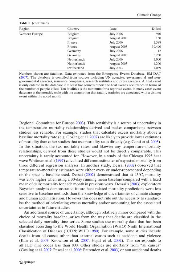
An indicative list of heat wave impacts for the period 2000–2007 is presented inTable 1 (EM-DAT 2007). France was one of the most severely affected countriesin the European August 2003 heat wave. Table 1 illustrates that there were vastlyfewer deaths in France during the 2006 heat wave, perhaps due to a reduction inheat wave intensity and a heat health watch warning system (French Institute forPublic Health Surveillance 2006; Pascal et al. 2006). However, Table 1 illustrates thatthe 2006 heat wave was associated with similar or more deaths than the 2003 eventin The Netherlands and Belgium respectively (EM-DAT 2007). This highlights theimportance of studies examining the association between elevated temperature andmortality, and the need to build on the coverage received in the IPCC AssessmentReports (IPCC 2001, 2007a) with an up-to-date review of the literature concerned.
This review differs from previous works that have focussed purely on epidemio-logical studies (Basu and Samet 2002). Such epidemiological studies seek to investi-gate and quantify the various risk factors that affect temperature-related mortality.These factors may include air pollution and socioeconomic status for example. Herea more holistic approach has been adopted because we also include studies where thefocus is shifted away from understanding the various mortality risk factors, towardsa focus on describing the relationship between atmospheric temperature and othermeteorological variables and mortality, and how this relationship may be affected byclimate change. This approach highlights the inter-disciplinary nature of the topic.The first section examines present temperature–mortality relationships as examinedby epidemiological and synoptic climatological methods, while the second sectiondiscusses climate change issues and examines the impacts of climate change onheat-related mortality. A unique element of the review is the critical appraisal ofmethodological issues, which precedes a presentation of the main research findings.Further research needs are highlighted throughout.
2 Review of present temperature–mortality relationships
2.1 Methodological approaches and related issues
2.1.1 Calculation of excess mortality
The majority of temperature–mortality studies do not use raw mortality data, but inorder to give an indication of the mortality attributable to temperature, calculatean excess mortality that is estimated by subtracting the expected mortality fromthe observed mortality. The expected mortality is often called the baseline mor-tality. Numerous methods have been identified in the literature for calculating the

Climatic Change
expected mortality, largely dependent upon the chosen baseline. These, and theirrespective advantages and disadvantages are summarised in Table 2. As a resultof these differences, mortality estimates are sensitive to the methods used (WHO
Table 1 Listof heat events by region and country during the period 2000–2007
Region Country Date Killed
North Africa Algeria July 2003 40Morocco August 2003
West Africa Nigeria June 2002 60North America US July–August 2006 24
US July–August 2006 164US July 2005 33US June 2002 14US August 2001 56US July 2000 35
East Asia China May–Sept 2006 134China July 2004 39China July 2002 7Japan July 2004 10Bangladesh May–June 2003 62India May 2006 47India June 2005 329India May–June 2003 1,210India May 2002 1,030India April 2000 7Pakistan May 2006 84Pakistan June 2005 106Pakistan May–June 2003 200Pakistan May 2002 113Pakistan June 2000 24
Western Asia Cyprus July 2000 5Turkey July 2000 15
Eastern Europe Bulgaria June–July 2000 8Romania June–July 2006 26Romania July–August 2005 13Romania July 2004 27Russia July 2001 276
Northern Europe UK August 2003 2,045Southern Europe Albania July 2004 3
Canary Islands July 2004 13Croatia July 2000 40Greece July 2000 3Italy July–August 2003 20,089Macedonia July 2004 15Portugal July 2006 41Portugal August 2003 2,007Serbia-Montenegro July 2000 3Spain July 2006 21Spain July 2004 26Spain August 2003 141
Climatic Change
Table 1 (continued)
Region Country Date Killed
Western Europe Belgium July 2006 940Belgium August 2003 150France July 2006 1,388France August 2003 19,490Germany July 2006 12Germany August 2003 5,250Netherlands July 2006 1,000Netherlands August 2003 1,200Switzerland July 2003 1,039
Numbers shown are fatalities. Data extracted from the Emergency Events Database, EM-DAT(2007). The database is compiled from sources including UN agencies, governmental and non-governmental agencies, insurance companies, research institutes and press agencies. A heat eventis only entered in the database if at least two sources report the heat event’s occurrence in terms ofthe number of people killed. Ten fatalities is the minimum for a reported event. In many cases eventdates are at the monthly scale with the assumption that fatality statistics are associated with a distinctevent within the noted month
Regional Committee for Europe 2003). This sensitivity is a source of uncertainty inthe temperature–mortality relationships derived and makes comparisons betweenstudies less reliable. For example, studies that calculate excess mortality above abaseline mortality rate (e.g. Gosling et al. 2007) are likely to provide lower estimatesof mortality than other studies that use mortality rates directly (e.g. Conti et al. 2005).In this situation, the two mortality rates, and likewise any temperature–mortalityrelationships, derived from these studies would not be directly comparable. Thisuncertainty is rarely accounted for. However, in a study of the Chicago 1995 heatwave Whitman et al. (1997) calculated different estimates of expected mortality fromthree different regression analyses. In another study, Dessai (2002) observed thattemperature–mortality estimates were either over- or under-represented dependingon the specific baseline used. Dessai (2002) demonstrated that at 43◦C, mortalitywas 20% higher when using a 30-day running mean baseline compared with a fixedmean of daily mortality for each month in previous years. Dessai’s (2003) exploratoryBayesian analysis demonstrated future heat-related mortality predictions were lesssensitive to baseline methods than the knowledge of uncertainties of climate changeand human acclimatisation. However this does not rule out the necessity to standard-ise the method of calculating excess mortality and/or accounting for the associateduncertainties in future studies.
An additional source of uncertainty, although relatively minor compared with thechoice of mortality baseline, arises from the way that deaths are classified in theselected daily mortality time series. Some studies use mortality data that has beenclassified according to the World Health Organisation (WHO) Ninth InternationalClassification of Diseases (ICD 9; WHO 1980). For example, some studies includedeaths from all causes other than external causes such as accidents and violence(Kan et al. 2007; Knowlton et al. 2007; Hajat et al. 2002). This corresponds toall ICD nine codes less than 800. Other studies use mortality from “all causes”(Gosling et al. 2007; Pascal et al. 2006; Pattenden et al. 2003) or non accidental deaths

Climatic Change
Tab
le2
Adv
anta
ges
and
disa
dvan
tage
sof
the
vari
ous
met
hods
for
calc
ulat
ing
exce
ssm
orta
lity
Met
hod
Ref
eren
ceA
dvan
tage
sD
isad
vant
ages
Com
pare
mor
talit
yw
ith
aba
selin
eD
onal
dson
etal
.(20
01,2
003)
Can
allo
wco
mpa
riso
nof
Mus
tacc
ount
for
fact
that
tem
pera
ture
sca
lcul
ated
asth
ete
mpe
ratu
rera
nge
exce
ssm
orta
lity
indi
ffer
ent
atw
hich
min
imum
mor
talit
yoc
curs
atw
hich
mor
talit
yis
ata
min
imum
geog
raph
ical
loca
tion
sw
illva
rysp
atia
llyan
dte
mpo
rally
Dai
lym
orta
lity
com
pare
dw
ith
31-o
rG
oslin
get
al.(
2007
)U
sefu
lwhe
relo
ngti
me
seri
es’
Incl
usio
nof
heat
wav
eda
ysin
the
mea
n30
-day
mov
ing
aver
age
for
the
sam
eye
arD
essa
i(20
02,2
003)
ofda
taar
eun
avai
labl
eva
lues
can
inhi
bitc
ompa
riso
nbe
twee
nR
oone
yet
al.(
1998
)di
ffer
ente
xtre
me
even
tsbe
caus
eof
diff
eren
ces
inth
eir
dura
tion
Dai
lym
orta
lity
com
pare
dw
ith
Huy
nen
etal
.(20
01)
Avo
ids
the
limit
atio
nas
soci
ated
wit
hE
xces
ses
atth
est
arto
fdat
ase
ts31
-or
30-d
aym
ovin
gav
erag
efo
rus
ing
am
ovin
gav
erag
ede
rive
dfr
omca
nnot
beca
lcul
ated
due
tono
data
2pr
eced
ing
year
sco
mbi
ned
the
sam
eye
aran
dm
ayth
eref
ore
bein
gav
aila
ble
for
prec
edin
gye
ars
beco
nsid
ered
mor
ere
liabl
eD
aily
mor
talit
yco
mpa
red
wit
hfix
edD
essa
i(20
02,2
003)
Can
beus
edif
few
year
sof
prev
ious
Exc
esse
sat
the
star
tofd
ata
sets
can
mea
nof
daily
mor
talit
yfo
rea
chm
onth
Jone
set
al.(
1982
)da
taar
eav
aila
ble
notb
eca
lcul
ated
due
tono
data
bein
gin
prev
ious
year
s(i
.e.f
orth
eba
selin
e,av
aila
ble
for
prec
edin
gye
ars
each
mon
thw
illha
veon
eva
lue)
Bas
elin
ege
nera
ted
byP
oiss
onL
eT
ertr
eet
al.(
2006
)A
llow
sm
odel
ling
ofin
here
ntse
ason
alM
ayno
tbe
appl
icab
leif
ther
ear
ere
gres
sion
and
non-
para
met
ric
Gem
mel
leta
l.(2
000)
patt
erns
inm
orta
lity
(sea
sona
lity)
and
limit
atio
nson
data
avai
labi
lity
smoo
thin
gte
chni
ques
Pál
dyet
al.(
2005
)ad
just
men
tsfo
rot
her
impo
rtan
tH
ajat
etal
.(20
02)
fact
ors
such
asin
fluen
zain
dica
tors
,W
hitm
anet
al.(
1997
)P
M10
,and
rela
tive
hum
idit
yG
uest
etal
.(19
99)
Cor
resp
ondi
ngda
yof
prev
ious
year
,C
onti
etal
.(20
05)
Can
beus
edif
few
year
sof
prev
ious
Bet
ter
tous
ea
larg
erda
tase
tifu
sing
this
orm
ean
from
seve
raly
ears
Mic
helo
zzie
tal.
(200
5)da
taar
eav
aila
ble
(e.g
.Con
tiet
al.
met
hod
(e.g
.Sar
tor
etal
.(19
95)
used
ON
S(2
003)
(200
5)us
ed1
year
—20
02)
1985
–199
3,an
dO
NS
(200
3)us
edSa
rtor
etal
.(19
95)
1998
–200
2)T
hem
edia
nm
orta
lity
for
the
mon
thD
avis
etal
.(20
03a,
b)Id
ealf
ora
non-
norm
alda
tase
tM
edia
nm
ayno
tbe
atr
uere
pres
enta
tion
inw
hich
the
deat
hsoc
curr
edis
subt
ract
edw
here
the
use
ofa
mon
thly
mea
nof
‘bas
elin
e’m
orta
lity
from
each
day’
sm
orta
lity
coun
tw
ould
notb
eap
prop
riat
eSu
btra
ctan
nual
mea
nfr
omm
onth
lyva
lue
Dav
iset
al.(
2004
)C
anbe
used
wit
hon
ly1
year
ofda
taB
ased
ona
limit
edti
me
peri
od

Climatic Change
(Kassomenos et al. 2007). Less common is the use of deaths certified as being“heat-related” (Whitman et al. 1997).
In a long time-series, the changing age–structure of the population should beaccounted for, because an ageing population will be more vulnerable and may biastemporal comparisons (Calado et al. 2005; Davis et al. 2003a). This is commonlyachieved by the direct standardisation method (Anderson and Rosenberg 1998),or by only examining a restricted age group. This method is commonly applied inthe epidemiological and synoptic climatological approaches. However, detailed andextensive datasets of daily mortality data stratified by age group are required for this,which is why a number of temperature–mortality assessments have not incorporatedthis standardisation method (Gosling et al. 2007; Casimiro et al. 2006; Dessai 2002).
2.1.2 The epidemiological approach
The epidemiological approach involves explaining an outcome measure (e.g. mor-tality) based upon a predictor(s) (e.g. temperature) and potentially confoundingvariables such as season, air pollution, other meteorological variables, and socio-economic status (Basu and Samet 2002). This can broadly be achieved by two mainmethods, (1) the analysis of time series data by Poisson regression and generalisedadditive models (GAMs), and (2) case-only or case-crossover studies. The principaldifference between the epidemiological approach and others such as the synopticclimatological approach is the consideration and modelling of various confoundingfactors in the former.
Poisson regression and GAMs relate the log-expected death count to the predic-tor(s) and confounders (Páldy et al. 2005; O’Neill et al. 2003; Pattenden et al. 2003;Curriero et al. 2002; Hajat et al. 2002). Daily temperature can be represented bylinear or non-linear terms in the models, on the same day or as lagged days (Bragaet al. 2001; Schwartz and Dockery 1992). Additional terms may be added to themodel to control for the confounding factors. This represents a major differencebetween the epidemiological and the synoptic climatological approach because inthe latter, the weather is not parameterised (Samet et al. 1998). A summary ofstudies that attempt to explain mortality as a function of temperature and othermeteorological and environmental variables is presented in Table 3. In some cases,socio-economic and/or lifestyle variables are also included; see Table 4.
Tables 3 and 4 illustrate that temperature is usually represented in terms ofminimum, maximum or mean daily temperature. However, very little attention ispaid to the explicit role of the diurnal temperature range (DTR). A recent exceptionis provided by Kan et al. (2007), who hypothesised that large diurnal temperaturechange might be a source of additional environmental stress, and therefore arisk factor for death. The 4-year study demonstrated significant increases in totalmortality associated with increases in daily DTR, independent of the correspondingtemperature level, in Shanghai on warm and cold days. The study acknowledges thattemperature level may modify the effect of DTR on mortality differently dependingon different weather patterns. Chen et al. (2007) made similar observations forstroke deaths in Shanghai. This novel risk factor deserves further research, especiallyas reductions in the DTR are projected with climate change (Meehl et al. 2007).The DTR is often included as a variable in the synoptic climatological approach,as discussed in the next section. Other studies calculate biometeorological indices

Climatic Change
Tab
le3
Stud
ies
inco
rpor
atin
gon
lyen
viro
nmen
talv
aria
bles
,inc
ludi
ngsu
mm
ary
offin
ding
sre
late
dto
the
vari
able
sex
amin
ed
Env
iron
men
talv
aria
bles
Ref
eren
ceC
ount
rySu
mm
ary
offin
ding
s
Dai
lym
orni
ngte
mpe
ratu
reD
avis
etal
.(20
04)
US
Rel
atio
nshi
pbe
twee
nm
onth
lym
orta
lity
and
tem
pera
ture
decr
ease
dbe
twee
n19
64an
d19
98(2
8U
Sci
ties
).C
oncl
uded
that
clim
ate
chan
gew
illha
velit
tle
effe
cton
mor
talit
yA
ppar
entt
empe
ratu
reW
hitm
anet
al.(
1997
)U
SN
osi
gnifi
cant
rela
tion
ship
betw
een
sum
mer
daily
tem
pera
ture
and
mor
talit
yov
er16
year
s(C
hica
go)
Dai
lym
inim
umte
mpe
ratu
reSc
hwar
tz(2
005)
US
Per
sons
wit
hdi
abet
esar
eat
high
erri
skto
deat
hon
hotd
ays,
and
pers
ons
wit
hch
roni
cob
stru
ctiv
epu
lmon
ary
dise
ase
(CO
PD
)to
deat
hon
cold
days
(Way
neC
ount
y,M
ichi
gan)
Dai
lyte
mpe
ratu
re,d
ewpo
int
Rob
erts
(200
4)U
SE
ffec
tofd
aily
PM
pollu
tion
may
depe
ndon
tem
pera
ture
(Coo
kte
mpe
ratu
re,a
ndP
M10
Cou
nty,
Illin
ois
and
Alle
ghen
yC
ount
y,P
enns
ylva
nia)
SSC
Kal
kste
inan
dG
reen
e(1
997)
US
Hig
hex
cess
mor
talit
yas
soci
ated
wit
ha
very
war
mm
oist
air
mas
san
da
hot,
dry
air
mas
s.So
uthe
rnci
ties
show
edw
eake
rre
lati
onsh
ips
insu
mm
er.B
y20
20an
d20
50,p
redi
cted
sum
mer
mor
talit
ym
uch
high
erth
anpr
esen
t,ev
enif
peop
leac
clim
atis
eD
aily
CE
T,N
O2,P
M10
Roo
ney
etal
.(19
98)
UK
Dai
lym
orta
lity
inE
ngla
ndan
dW
ales
duri
ng19
95he
atw
ave
rose
8.9%
abov
eth
ese
ason
alav
erag
e.A
irpo
lluti
onm
ayha
veac
coun
ted
for
upto
62%
ofex
cess
mor
talit
yM
ean
daily
tem
pera
ture
,rel
ativ
ehu
mid
ity,
Haj
atet
al.(
2002
)U
KM
orta
lity
high
erif
heat
wav
eoc
curs
earl
ier
insu
mm
erSO
2,O
3,a
ndbl
ack
smok
e(L
ondo
n,fo
r19
76–1
996)
.Air
pollu
tion
data
had
littl
ein
fluen
ceon
mor
talit
y.M
inim
umte
mpe
ratu
rein
fluen
ced
mor
talit
ym
ore
than
max
tem
pera
ture
CE
TD
onal
dson
etal
.(20
01)
UK
Ass
umin
gst
atio
nari
tyof
pres
entt
empe
ratu
re–m
orta
lity
rela
tion
ship
san
dno
accl
imat
isat
ion,
a25
3%in
crea
sein
heat
-rel
ated
mor
talit
ypr
edic
ted
for
2050
sbu
tade
clin
ein
win
ter
mor
talit
y(U
K)
Mea
nda
ilyte
mpe
ratu
re,w
ind
Don
alds
onet
al.(
2003
)U
KM
orta
lity
mor
ese
nsit
ive
toco
ldin
war
mer
regi
ons
(Nor
thC
arol
ina)
spee
dan
dre
lati
vehu
mid
ity
US
than
cool
eron
es(S
.E.E
ngla
nd)
and
vice
vers
a.O
ther
vari
able
sF
inla
ndon
lyus
edfo
rqu
alit
ativ
ean
alys
is.A
nnua
lhea
t-re
late
dm
orta
lity
decl
ined
betw
een
1971
and
1997
for
alll
ocat
ions

Climatic Change
Tab
le3
(con
tinu
ed)
Env
iron
men
talv
aria
bles
Ref
eren
ceC
ount
rySu
mm
ary
offin
ding
s
Mea
nda
ilyte
mpe
ratu
re,r
elat
ive
Pat
tend
enet
al.(
2003
)U
KSi
gnifi
cant
tem
pera
ture
–mor
talit
yas
soci
atio
ns(L
ondo
nan
dSo
fia).
hum
idit
y,an
dpa
rtic
ulat
em
atte
rB
ulga
ria
Eff
ecto
fcol
dgr
eate
rin
city
wit
hw
arm
ercl
imat
e(L
ondo
n).
Par
ticu
late
mat
ter
sign
ifica
ntly
effe
cted
mor
talit
yin
Sofia
but
notL
ondo
nD
aily
mea
n,m
axim
um,m
inim
um,
Haj
atet
al.(
2006
)U
KE
xam
ined
the
“hea
twav
eef
fect
”,i.e
.the
extr
ade
aths
occu
rrin
gan
dap
pare
ntte
mpe
ratu
re,
Hun
gary
abov
ew
hatw
ould
beex
pect
edfr
oma
smoo
thte
mpe
ratu
re–m
orta
lity
blac
ksm
oke
and
ozon
eIt
aly
grad
ient
rela
tion
ship
,due
toco
nsec
utiv
eda
ysof
high
tem
pera
ture
s(h
eatw
aves
).A
nad
diti
onal
“hea
twav
e”ef
fect
of5.
5%w
asob
serv
edin
inL
ondo
n(1
976–
2003
),9.
3%in
Bud
apes
t(19
70–2
000)
,and
15.2
%in
Mila
n(1
985–
2002
).D
aily
mea
nte
mpe
ratu
rega
veth
ebe
stfit
tom
orta
lity
Mea
nda
ilyte
mpe
ratu
re,p
ress
ure,
Pál
dyet
al.(
2005
)H
unga
ry5◦
Cin
crea
sein
tem
pera
ture
incr
ease
dri
skof
tota
lmor
talit
yby
10.6
%re
lati
vehu
mid
ity,
PM
10in
Bud
apes
t.R
elat
ions
hip
betw
een
PM
10an
dm
orta
lity
wer
ew
eake
r.F
irst
heat
wav
ein
aye
arha
shi
ghes
tmor
talit
y-im
pact
Mea
nda
ilyte
mpe
ratu
re,r
elat
ive
Bal
lest
eret
al.(
1997
)Sp
ain
Sign
ifica
ntte
mpe
ratu
re–m
orta
lity
rela
tion
ship
sin
Val
enci
a,an
nual
ly,
hum
idit
y,an
dsu
spen
ded
part
icul
ates
and
inw
inte
ran
dsu
mm
erm
onth
sre
spec
tive
ly.I
nflue
nce
ofhu
mid
ity
foun
dto
bein
sign
ifica
ntM
ean
daily
tem
pera
ture
,rel
ativ
eSa
ezet
al.(
2000
)Sp
ain
Hum
idit
yin
fluen
ced
the
tem
pera
ture
atw
hich
the
onse
thu
mid
ity,
blac
ksm
oke,
SO2,O
3,N
O2
ofex
cess
isch
aem
iche
artd
isea
sede
aths
occu
rred
(Bar
celo
na)
Hum
idex
inde
x(a
func
tion
ofC
onti
etal
.(20
05)
Ital
y92
%of
exce
ssde
aths
insu
mm
er20
03he
atw
ave
wer
eam
ongs
teld
erly
.te
mpe
ratu
rean
dva
pour
pres
sure
)L
arge
stex
cess
esw
ere
inth
eno
rthw
este
rn,c
oole
rci
ties

Climatic Change
TSI
and
blac
ksm
oke
Kas
som
enos
etal
.(20
07)
Gre
ece
Six
air
mas
ses
wer
eob
serv
edfo
rth
ew
arm
mon
ths
(Apr
il-O
ctob
er)
for
Ath
ens,
1987
–199
1.T
hem
ostu
nfav
oura
ble
tom
orta
lity
was
asso
ciat
edw
ith
ase
abr
eeze
that
prom
oted
war
man
dhu
mid
cond
itio
ns.T
hese
asso
ciat
ions
wer
ein
depe
nden
tofb
lack
smok
eco
ncen
trat
ions
Mea
nda
ilyte
mpe
ratu
reH
uyne
net
al.(
2001
)N
ethe
rlan
dsL
arge
stex
cess
mor
talit
yas
soci
ated
wit
hlo
nges
tlas
ting
heat
wav
es(N
ethe
rlan
ds).
Som
efo
rwar
ddi
spla
cem
ento
fdea
ths
duri
nghe
atw
aves
butn
otdu
ring
cold
spel
lsM
ean
daily
tem
pera
ture
and
Des
sai(
2002
,200
3)P
ortu
gal
Sign
ifica
ntte
mpe
ratu
re–m
orta
lity
rela
tion
ship
sob
serv
edin
Lis
bon
rela
tive
hum
idit
yfo
rpe
riod
1980
–199
8.R
elat
ive
hum
idit
yw
asno
tsig
nific
ant
Mea
nda
ilyte
mpe
ratu
re,r
elat
ive
Sart
oret
al.(
1995
)B
elgi
umM
ostl
ikel
yca
uses
ofel
evat
edex
cess
mor
talit
ydu
ring
Sum
mer
hum
idit
y,su
spen
ded
part
icul
ates
,19
94in
Bel
gium
wer
ehi
ghou
tdoo
rte
mpe
ratu
res
com
bine
dSO
2,O
3,N
O2,N
Ox
wit
hhi
ghoz
one
conc
entr
atio
nsM
inim
umte
mpe
ratu
reon
the
curr
entd
ay,
Le
Ter
tre
etal
.(20
06)
Fra
nce
Usu
alai
rpo
lluti
onan
dte
mpe
ratu
reef
fect
sdi
dno
tapp
ear
asth
em
axim
umte
mpe
ratu
reon
the
mai
nfa
ctor
saf
fect
ing
mor
talit
yin
9ci
ties
duri
ngth
e20
03pr
evio
usda
y,O
3F
ranc
ehe
atw
ave.
3,09
6ex
tra
deat
hsw
ere
esti
mat
edto
have
resu
lted
from
the
heat
wav
e.L
ittl
eev
iden
ceof
mor
talit
ydi
spla
cem
ent
Diu
rnal
tem
pera
ture
rang
e(D
TR
),K
anet
al.(
2007
)C
hina
A1◦
Cin
crem
ento
fthe
3-da
ym
ovin
gav
erag
eof
DT
Rco
rres
pond
edto
PM
10,S
O2,O
3,N
O2
a1.
37%
incr
ease
into
talm
orta
lity
(Sha
ngha
i,20
01–2
004)
.U
ncer
tain
whe
ther
air
pollu
tion
vari
able
sw
ere
conf
ound
ers
oref
fect
mod
erat
ors
ofth
eD
TR
–mor
talit
yas
soci
atio
n

Climatic Change
Tab
le4
Stud
ies
inco
rpor
atin
gen
viro
nmen
tala
ndso
cio-
econ
omic
/life
styl
eva
riab
les,
incl
udin
gsu
mm
ary
offin
ding
sre
late
dto
the
vari
able
sex
amin
ed
Env
iron
men
talv
aria
bles
Soci
oec
onom
ic/
Ref
eren
ceC
ount
rySu
mm
ary
offin
ding
slif
esty
leva
riab
les
TSI
,sus
pend
edpa
rtic
ulat
es,
Rac
eK
alks
tein
(199
1)U
SD
aily
mor
talit
ym
ore
sens
itiv
eto
stre
ssfu
lwea
ther
than
tota
loxi
dant
s,SO
2,O
3,
high
pollu
tion
leve
ls(S
tLou
is).
Lon
gco
nsec
utiv
eda
ysN
Ox,N
O2
ofho
t,tr
opic
alop
pres
sive
wea
ther
asso
ciat
edw
ith
elev
ated
exce
ssm
orta
lity,
part
icul
arly
amon
gel
derl
yan
dno
n-w
hite
s.M
axim
umte
mpe
ratu
rew
asno
tasi
gnifi
cant
fact
or(m
inim
umte
mpe
ratu
rew
as)
TSI
Stan
dard
ofliv
ing,
Che
snut
etal
.(19
98)
US
Soci
oec
onom
icfa
ctor
sex
plai
ned
less
heat
rela
ted
air
cond
itio
ning
,m
orta
lity
vari
atio
nth
anva
riab
ility
inda
ilym
inim
umho
usin
gqu
alit
y,te
mpe
ratu
re(4
4U
Sm
etro
polit
anar
eas)
.Str
onge
stpo
pula
tion
dens
ity
tem
pera
ture
mor
talit
yre
lati
onsh
ips
occu
rred
inno
rthe
rnar
eas,
even
thou
ghso
uthe
rnar
eas
wer
ew
arm
erD
aily
min
imum
Rac
e(w
hite
orSc
hwar
tz(2
005)
US
Non
whi
tes
had
agr
eate
rri
skof
mor
talit
yon
hota
ndte
mpe
ratu
reno
nw
hite
)co
ldda
ys(W
ayne
Cou
nty,
Mic
higa
n)M
ean
daily
tem
pera
ture
,A
irco
ndit
ioni
ngB
raga
etal
.(20
01)
US
Var
ianc
eof
sum
mer
tim
ete
mpe
ratu
res
expl
aine
dm
ore
rela
tive
hum
idit
y,va
riat
ion
inhe
atre
late
dm
orta
lity
risk
(64%
)th
anai
ran
dpr
essu
reco
ndit
ioni
ng(3
3%)
for
12U
Sci
ties
.Hum
idit
yno
tsi
gnifi
cant
.No
tem
pera
ture
mor
talit
yas
soci
atio
nsin
citi
esw
ith
hott
estc
limat
es,m
eani
ngth
atre
lati
onsh
ips
wer
eei
ther
‘V-’
or‘J
-’sh
aped
depe
ndin
gon
city
Mea
nda
ilyte
mpe
ratu
reC
ompl
etin
ghi
ghsc
hool
,C
urri
ero
etal
.(20
02)
US
Gre
ater
effe
ctof
cold
onm
orta
lity
risk
inso
uthe
rnci
ties
and
dew
poin
ttem
pera
ture
livin
gin
pove
rty,
and
ofw
arm
thin
nort
hern
citi
es.A
irco
ndit
ioni
ngan
dai
rco
ndit
ioni
ng,h
eati
ng,
heat
ing
wer
esi
gnifi
cant
prev
enta
tive
fact
ors
inso
uth
aged
65+
wit
hdi
sabi
lity
and
nort
hre
spec
tive
ly

Climatic Change
Dai
lyap
pare
ntte
mpe
ratu
re,
Air
cond
itio
ning
Dav
iset
al.(
2003
a)U
SH
eat-
rela
ted
mor
talit
yde
clin
edin
19/2
8U
Sci
ties
tem
pera
ture
,dew
betw
een
1964
–199
8an
dw
asas
soci
ated
wit
hai
rpo
intt
empe
ratu
reco
ndit
ioni
ngav
aila
bilit
y.So
uthe
rnci
ties
exhi
bite
dw
eake
rho
ttem
pera
ture
mor
talit
yre
lati
onsh
ips.
Tem
pera
ture
vari
abili
tyw
asin
sign
ifica
ntA
ppar
entt
empe
ratu
reD
emog
raph
ic,s
ocio
Smoy
eret
al.(
2000
a)U
SG
reat
esth
eatr
elat
edm
orta
lity
was
inci
ties
wit
hhi
ghec
onom
ic,a
ndur
bani
sati
onan
dco
sts
ofliv
ing
(Sou
ther
nO
ntar
io)
hous
ing
fact
ors
Wee
kly
mea
nte
mpe
ratu
reR
egis
trar
Gen
eral
’sso
cial
Gem
mel
leta
l.(2
000)
Scot
land
Seas
onal
wee
kly
deat
hra
tes
high
erin
win
ter
than
clas
ses
(Sco
tlan
d),a
rea
sum
mer
inSc
otla
ndbu
tno
rela
tion
ship
betw
een
base
dde
priv
atio
ngr
oups
soci
oec
onom
icst
atus
and
seas
onal
mor
talit
yD
aily
appa
rent
tem
pera
ture
.E
duca
tion
,occ
upat
ion,
Mic
helo
zzie
tal.
(200
5)It
aly
Gre
ates
texc
ess
mor
talit
ydu
eto
heat
wav
esM
ean,
max
imum
and
unem
ploy
men
t,in
Rom
ean
dT
urin
wer
ein
low
est
min
imum
tem
pera
ture
num
ber
offa
mily
mem
bers
,so
cio
econ
omic
leve
lpop
ulat
ions
over
crow
ding
,and
hous
ehol
dow
ners
hip
TSI
,tem
pera
ture
,dry
and
Hou
seho
ldec
onom
icG
uest
etal
.(19
99)
Aus
tral
iaA
irm
asse
sas
soci
ated
wit
hhi
ghdr
ybu
lban
dde
wpo
int
wet
bulb
tem
pera
ture
,re
sour
ces,
educ
atio
n,te
mpe
ratu
res
asso
ciat
edw
ith
high
estm
orta
litie
sde
wpo
int,
win
dsp
eed,
occu
pati
on,f
amily
acro
ss5
Aus
tral
ian
citi
es.1
0%re
duct
ion
inpr
essu
re,c
loud
cove
rst
ruct
ure,
ethn
icit
ym
orta
lity
was
pred
icte
dby
2030
.Soc
ioec
onom
icst
atus
had
littl
ein
fluen
ceon
rela
tion
ship
sD
aily
max
imum
tem
pera
ture
,A
irco
ndit
ioni
ng,l
ivin
gT
anet
al.(
2007
)C
hina
Pol
luti
onva
riab
les
less
stro
ngly
asso
ciat
edw
ith
mor
talit
yP
M10
,SO
2,N
O2
spac
e,ur
ban
gree
nth
ante
mpe
ratu
redu
ring
heat
wav
esoc
curr
ing
area
cove
rage
in19
98an
d20
03in
Shan
ghai
,and
the
rela
tive
cont
ribu
tion
sof
each
wer
eun
cert
ain.
Incr
ease
sin
air
cond
itio
ning
and
urba
ngr
een
spac
ew
ere
thou
ght
tobe
impo
rtan
tin
redu
cing
mor
talit
y.C
umul
ativ
eho
tday
sw
ere
mor
ede
adly
than
isol
ated
hotd
ays

Climatic Change
such as the apparent temperature (Hajat et al. 2006; Michelozzi et al. 2005; Daviset al. 2003a; Smoyer et al. 2000a) or humidex (Conti et al. 2005). These indicesare absolute so that they assume the weather has the same impact on the humanbody regardless of location or the time at which it occurs. Therefore there has beenrecent interest in the computation of relative biometeorological indices such as theheat stress index (Watts and Kalkstein 2004) that is based on apparent temperature,cloud cover, and consecutive days, and HeRATE (Health Related Assessment ofthe Thermal Environment) that combines a physiologically relevant assessmentprocedure of the thermal environment with a conceptual model to describe short-term adaptation (including short-term acclimatisation and behavioural adaptation)to the thermal conditions of the past 4 weeks (Koppe and Jendritzky 2005). Otherstudies prefer only to examine temperature–mortality associations above a specificthreshold (e.g. the 95th percentile of daily temperature; Gosling et al. 2007; Hajatet al. 2002)—this is discussed in more detail in Section 2.1.4.
The epidemiological approach can be applied to isolated events such as heatwaves (Calado et al. 2005; Conti et al. 2005; Michelozzi et al. 2005; Smoyer 1998)or over longer periods that use time-series data (Hajat et al. 2005, 2006; Pattendenet al. 2003; Dessai 2002; Gemmell et al. 2000; Danet et al. 1999; Ballester et al.1997). Although the analysis of isolated heat waves provides a useful insight into theshort-term response of the population to the event, they can overestimate the effectof temperature due to short-term mortality displacements (Sartor et al. 1995) andinappropriate use of mortality baselines (Rooney et al. 1998; Whitman et al. 1997).An increasingly popular and more objective method to examine the temperature–mortality association is to investigate long-period time-series data through regressionanalysis, and then identify individual events such as heat waves in that time-series forfurther analysis (Páldy et al. 2005; Hajat et al. 2002; Huynen et al. 2001).
There are limitations in including environmental variables under the epidemio-logical approach. Firstly, a single weather element may not be representative of thetotal effect of weather on health because other meteorological variables can affecthuman health synergistically (Kalkstein 1991). However, there is some evidence thatindividual elements such as humidity have no significant relationship with mortality(Dessai 2002, 2003; Ballester et al. 1997; Braga et al. 2001). Secondly, measurementsof meteorological variables are often obtained from point-source weather stationsthat may be some distance from where the health effects are recorded, and moreimportantly, may not be representative of the conditions within the buildings wheremost deaths occur (Kilbourne 1997). Thirdly, it is possible that mortality variationis pollution-orientated (Kalkstein 1991), but the inclusion of individual pollutantvariables and weather variables as additive independent variables is unjustifiedbecause of the possibility of collinearity between the two (Roberts 2004; Sartor et al.1995). Nevertheless, the degree to which air pollution effects mortality deservesfurther research, since attribution to this is uncertain (Kan et al. 2007; Pattendenet al. 2003; Hajat et al. 2002; Keatinge and Donaldson 2001; Smoyer et al. 2000b). Theproblem of collinearity may also arise when including non-environmental variablesin temperature–mortality regression models. For example, Chesnut et al. (1998)observed a statistically significant negative relationship between percentage of thepopulation that graduated from high school and hot-weather-related mortality. Itshould be noted that the relationship is not necessarily causal, and may be explaineddue to the correlation between high school graduation and income, such that

Climatic Change
wealthier populations can take more preventative action against adverse conditions(e.g. air conditioning) (Semenza et al. 1996). Hence regression coefficients for onevariable may be a reflection of the influence of any other correlated variable, soresults should be treated with caution. It is perhaps due to this limitation thatthere is a marked variation in the degree to which socio-economic factors and/orlifestyle variables are related to heat-related mortality (Michelozzi et al. 2005; Guestet al. 1999). Compounding this limitation is the use of different indicators of socio-economic status, which impedes cross-study comparisons.
The case-only or case-crossover epidemiological approach allows examination ofthe relationship between an acute event and a quick-changing risk factor by includingonly people that experience the acute event in the analysis (Maclure 1991). Basuand Samet (2002) describe the approach as being where two or more time periodsare defined for each person experiencing the outcome. One of these is the “hazardperiod” that represents the exposure period to the acute event. The other periodconsists of one or more “control periods” that represent the exposure experiencedbefore and/or after the hazard period. However, this means that the date of deathfor each individual is required—something that is not always available (Basu 2001).Armstrong (2003) has noted how this method can be used to examine the acuteeffects of weather, such that the limitation of socio-economic variable-collinearityin GAMs can to some extent be resolved because complex modelling of confoundersis not required. This is mainly because the individuals under examination also act astheir own control; i.e. before and after the acute event (Schwartz 2005; Semenza et al.1996; Kilbourne et al. 1982). This approach is therefore useful for future studies, butthey must account for two important factors: firstly the Neyman bias (Redelmeierand Tibshirani 1997): a circumstance in which deaths occur due to more severecauses, but are not attributed to heat stress (the outcome of interest), and secondly, aneed to control for seasonal interactions that could have implications for how reliabletemperature-susceptibility measures are (Armstrong 2003). It should be noted thatalthough this approach is useful for monitoring at-risk groups, preventative measuresshould be aimed at the population as a whole, as well as particularly vulnerablegroups (Ballester et al. 1997).
2.1.3 The synoptic climatological approach
The limitations associated with environmental variables under the epidemiologicalapproach can to some extent, be alleviated by adopting a synoptic climatologicalapproach. This uses principal components analysis (PCA) and cluster analysis (CA)to group daily homogenous meteorological variables in to air mass groups. Theresult is a temporal synoptic index (TSI) that can be compared with daily mortality(Kalkstein 1991; Kalkstein and Smoyer 1993; Greene and Kalkstein 1996; Chesnutet al. 1998; Guest et al. 1999; Kassomenos et al. 2007). However, a limitation ofthe TSI is that it is location-specific. Air masses are defined without regard to otherplaces, meaning the ‘oppressive’ air mass groups identified for one region may bedifferent to those for another, which renders regional comparisons problematic. Thisproblem has been overcome by applying a methodology that identifies the majorair masses traversing a particular region, to produce a spatial synoptic classification(SSC) (Kalkstein and Greene 1997; Sheridan and Kalkstein 2004). This has been

Climatic Change
refined as the SSC2 for use across North America (Sheridan 2002). However, Guestet al. (1999) argue that it is always possible that TSI– or SSC–mortality associationsmay arise partly from confounding factors.
McMichael et al. (1996) have illustrated the usefulness of the TSI in climate–healthresearch and Guest et al. (1999) concluded the TSI was the most comprehensivemethod for examining climate–mortality relationships in Australia over the period1979–1990, compared with the epidemiological approach of non-linear regressionand correlation analyses. However, Samet et al. (1998) compared the TSI approachwith linear and non-linear regression methods, concluding that the inclusion ofparametric or smoothed terms to control for the weather in Philadelphia during theperiod 1973–1980 were superior. Nevertheless the practical benefits of the synopticapproach have been realised through the development of numerous heat healthwatch warning systems in cities such as Shanghai, Toronto, Rome, and Chicago(Sheridan and Kalkstein 2004). Until recently, the synoptic climatological approachhas rarely been adopted outside of the US, but McGregor (1999) has applied themethodology to examine winter ischaemic heart disease in Birmingham (UK) andKassomenos et al. (2007) have examined heat stress in Athens (Greece). Also, Boweret al. (2007) have developed a new SSC for Western Europe (SSCWE) based on datafrom 48 weather stations over the period 1974–2000. Similar studies in Europe andthe developing world would advance the climate–health knowledge base.
2.1.4 Defining heat waves
A major issue of debate is how “hot days” or heat waves should be defined. Robinson(2001) defines a heat wave as “an extended period of unusually high atmosphere-related heat stress, which causes temporary modifications in lifestyle, and which mayhave adverse health consequences for the affected population.” Therefore althoughheat waves are meteorological events, they are more usefully defined with referenceto human impacts. Considering this, Robinson (2001) accounts for intensity andduration and proposes heat waves in the US should be defined as periods of atleast 2 days when absolute thresholds of daytime high and nighttime low apparenttemperature are exceeded. A similar definition is adopted by the Netherlands RoyalMeteorological Institute, which defines a heat wave as a period of at least 5 days,each of which has a maximum temperature of 25◦C or higher, including at least3 days with a maximum temperature of 30◦C or higher (Huynen et al. 2001). Tanet al. (2007) defined hot days in Shanghai as when the daily maximum temperatureexceeded 35◦C, to correspond with the Chinese Meteorological Administration heatwarnings that are issued when maximum temperatures are forecast to exceed 35◦C.
However, absolute thresholds such as these cannot be applied directly elsewherebecause the sensitivity of populations to heat will vary spatially. For example, incooler regions the thresholds may never be reached, and the thresholds may haveto be higher in hotter regions to ensure only those events perceived as stressfulare identified. The UK Met Office’s Heat–Health Watch system (Department ofHealth 2007) deals with this by issuing health alerts based upon whether thresholdmaximum daytime and minimum night-time temperatures, which vary by region, arereached on at least two consecutive days and the intervening night. For example thethresholds for London are 32◦C (day) and 18◦C (night) but the thresholds for NorthEast England are 28◦C (day) and 15◦C (night).

Climatic Change
These spatial differences are accounted for elsewhere by defining the intensity byusing temperature percentiles. Beniston (2004) defines heat waves as three succes-sive days when the temperature exceeds the 90th percentile of summer maximumtemperature, because this corresponds to the extreme high tail of probability densityfunction of maximum summer temperature as defined by the IPCC (2001). Hajatet al. (2002) defined heat waves as periods of five consecutive days or longer whena smoothed 3-day moving average of temperature exceeded the 97th percentileof average temperature for the entire period. Gosling et al. (2007) defined heatwaves as periods lasting three or more consecutive days when the daily maximumtemperature was equal to, or greater than, the 95th percentile of summer maximumtemperature over the whole period of record. Although the use of percentiles inthis manner allows for regional differences in sensitivity, it does not account forseasonal changes in the sensitivity. Furthermore it remains possible that in somevery cool locations with little temperature variability, a threshold such as the 99thpercentile may produce no appreciable increase in mortality. Regarding the duration,it is rarely justified why the chosen percentile should be exceeded for how evermany days. The importance of the duration of stressful weather conditions has beenhighlighted by studies adopting a synoptic climatological approach. Sheridan andKalkstein (2004) have demonstrated for Toronto that although increases in mortalitymay be statistically significant on the first day of an oppressive weather type (drytropical), they may increase up to tenfold if the offensive weather type persists forfive consecutive days. Furthermore, Kyselý (2007) has demonstrated that surfaceair temperature anomalies over Europe are linked to the persistence of certaincirculation patterns over Europe, and that the occurrence and severity of temper-ature extremes (heat and cold) become more pronounced under a more persistentcirculation. The longer continuous exposure to oppressive weather places additionalstress upon the human body. A heat wave definition that considers the TSI/SSCmethodology would therefore be useful. Although a common, formal definition ofa heat wave for a wide area such as Europe is desirable, it is the limitations discussedhere that hinder its formulation, and is perhaps why no common, formal definitionof a heat wave currently exists (Koppe et al. 2004).
2.2 Findings
Both warm and cold extremes of temperature have adverse effects on health,such that a non-monotonic relationship is often observed between temperature andmortality, with a temperature band of minimum mortality. This band is sometimesreferred to as the ‘comfort range’ (Martens 1998), the limits of which representthe ‘threshold temperature’. Beyond this mortality increases above the baselinelevel (Kalkstein and Davis 1989). A summary of observed threshold temperaturesis presented in Table 5, which also highlights that different thresholds have beenidentified for different causes of death. Furthermore, threshold values may beconfounded by other meteorological variables—for example, Saez et al. (2000)illustrated a 2◦C higher threshold (23◦C) on very humid days (when the relativehumidity was above 85%) compared to less humid days in Barcelona, Spain. Thisis interesting because a lower threshold temperature might be expected with higherhumidity because high humidity increases heat stress by hindering the evaporation

Climatic Change
Tab
le5
Evi
denc
efo
rte
mpe
ratu
reba
nds
ofm
inim
umm
orta
lity
inor
der
ofde
crea
sing
dist
ance
from
the
Equ
ator
,inc
ludi
ngag
egr
oups
exam
ined
,cau
ses
ofde
ath,
and
natu
reof
rela
tion
ship
s(i
fsta
ted
inst
udy)
Loc
atio
nT
empe
ratu
reof
min
imum
mor
talit
y(◦
C)
Ref
eren
ceN
otes
Nor
thF
inla
nd14
.3–1
7.3
Kea
ting
eet
al.(
2000
)A
ge65
–74,
1988
–199
2.F
or1◦
Cin
crea
se/d
ecre
ase
abov
e/be
low
min
imum
mor
talit
yba
nd,t
otal
mor
talit
yin
crea
sed
by6.
2/0.
58de
aths
per
mill
ion
per
day
Nor
thF
inla
nd18
.0E
urow
inte
r(1
997)
Age
50–5
9,65
–74,
and
alla
ges,
1988
–199
2.IH
D,C
VD
,RD
,and
tota
lmor
talit
y.M
ean
incr
ease
into
talm
orta
lity/
1◦C
fall
belo
w18
◦ Cw
as0.
29%
for
Nor
thF
inla
ndSo
uth
Fin
land
12.2
–15.
2D
onal
dson
etal
.(20
03)
Tot
alm
orta
lity,
age
over
55,1
971–
1997
UK
15.6
–18.
6D
onal
dson
etal
.(20
01)
Tot
alm
orta
lity,
alla
ges,
1976
–199
6N
ethe
rlan
ds14
.5H
uyne
net
al.(
2001
)T
otal
mor
talit
y,ag
e0–
64,1
979–
1997
Net
herl
ands
15.5
Huy
nen
etal
.(20
01)
Thr
esho
ldis
for
mal
igna
ntne
opla
sms,
age
over
65,1
979–
1997
.F
or1◦
Cin
crea
se/d
ecre
ase
abov
e/be
low
15.5
◦ C,m
alig
nant
neop
lasm
sm
orta
lity
incr
ease
dby
0.47
%/0
.22%
Net
herl
ands
16.5
Huy
nen
etal
.(20
01)
Thr
esho
ldis
for
tota
lmor
talit
y,C
D,R
D,a
geov
er65
,197
9–19
97.
For
1◦C
incr
ease
abov
e16
.5◦ C
;CD
,RD
,and
tota
lmor
talit
yin
crea
sed
by1.
86%
,12.
82%
and
2.72
%re
spec
tive
ly.F
or1◦
Cde
crea
sebe
low
16.5
◦ C;C
D,R
D,a
ndto
talm
orta
lity
incr
ease
dby
1.69
%,5
.15%
,and
1.37
%re
spec
tive
lyN
ethe
rlan
ds18
.0E
urow
inte
r(1
997)
Age
50–5
9,65
–74,
and
alla
ges,
1988
–199
2.IH
D,C
VD
,RD
,and
tota
lmor
talit
y.M
ean
incr
ease
into
talm
orta
lity/
1◦C
fall
belo
w18
◦ Cw
as0.
59%
for
Net
herl
ands
Sout
heas
tEng
land
15.0
–18.
0D
onal
dson
etal
.(20
03)
Tot
alm
orta
lity,
age
over
55,1
971–
1997
Lon
don,
UK
18.0
Pat
tend
enet
al.(
2003
)T
otal
mor
talit
y,al
lage
s,19
93–1
996.
Incr
easi
ng/d
ecre
asin
gte
mpe
ratu
reas
soci
ated
wit
ha
mor
talit
ych
ange
of+
1.30
%/+
1.43
%pe
r1◦
Cte
mpe
ratu
reri
se/f
alla
bove
/bel
ow18
◦ C

Climatic Change
Lon
don,
UK
18.0
Eur
owin
ter
(199
7)A
ge50
–59,
65–7
4,an
dal
lage
s,19
88–1
992.
IHD
,CV
D,
RD
,and
tota
lmor
talit
y.M
ean
incr
ease
into
tal
mor
talit
y/1◦
Cfa
llbe
low
18◦ C
was
1.37
%fo
rL
ondo
nL
ondo
n,U
K19
.0G
oslin
get
al.(
2007
)T
otal
mor
talit
y,al
lage
s,19
76–2
003
(Gos
ling
etal
.200
7)H
ajat
etal
.(20
02)
Tot
alm
orta
lity
(com
pris
ing
RD
and
CD
),al
lage
s,19
76–1
996—
abov
e21
.5◦ C
(97t
hpe
rcen
tile
valu
e),
3.34
%in
crea
sein
deat
hs/1
◦ Cri
sein
tem
pera
ture
(Haj
atet
al.2
002)
Lon
don,
UK
19.3
–22.
3K
eati
nge
etal
.(20
00)
Age
65–7
4,19
88–1
992.
For
1◦C
incr
ease
/dec
reas
eab
ove/
belo
wm
inim
umm
orta
lity
band
,tot
alm
orta
lity
incr
ease
dby
3.6/
1.25
deat
hspe
rm
illio
npe
rda
yL
ondo
n,U
K20
.5H
ajat
etal
.(20
06)
Tot
alm
orta
lity,
alla
ges,
1976
–200
3.M
orta
lity
incr
ease
d4.
5%fo
rev
ery
degr
eein
crea
sein
tem
pera
ture
abov
eth
resh
old
Par
is,F
ranc
e20
.6–2
3.6
Laa
idie
tal.
(200
6)T
otal
mor
talit
y,al
lage
s,19
91–1
995
Bud
apes
t,H
unga
ry18
.0P
áldy
etal
.(20
05)
All
ages
,197
0–20
00.F
or5◦
Cin
crea
sein
tem
pera
ture
abov
eth
resh
old,
risk
ofto
talm
orta
lity
incr
ease
dby
10.6
%(t
otal
mor
talit
y),1
8%(C
D),
8.8%
(RD
)B
udap
est,
Hun
gary
19.6
Haj
atet
al.(
2006
)T
otal
mor
talit
y,al
lage
s,19
70–2
000.
Mor
talit
yin
crea
sed
2.7%
for
ever
yde
gree
incr
ease
inte
mpe
ratu
reab
ove
thre
shol
dM
ilan,
Ital
y23
.4H
ajat
etal
.(20
06)
Tot
alm
orta
lity,
alla
ges,
1985
–200
2.M
orta
lity
incr
ease
d4.
8%fo
rev
ery
degr
eein
crea
sein
tem
pera
ture
abov
eth
resh
old
Sofia
,Bul
gari
a18
.0P
atte
nden
etal
.(20
03)
Tot
alm
orta
lity,
alla
ges,
1993
–199
6.In
crea
sing
/dec
reas
ing
tem
pera
ture
asso
ciat
edw
ith
am
orta
lity
chan
geof
+2.
21%
/+0.
70%
per
1◦C
tem
pera
ture
rise
/fal
labo
ve/b
elow
18◦ C
Bos
ton,
US
22.0
Gos
ling
etal
.(20
07)
Tot
alm
orta
lity,
alla
ges,
1975
–199
8B
arce
lona
,Spa
in21
.06
Saez
etal
.(20
00)
Age
over
45,1
986–
1991
(thr
esho
ldhi
gher
(23◦
C)
onve
ryhu
mid
days
[rel
ativ
ehu
mid
ity
over
85%
]).R
isk
ofIH
Dde
ath
incr
ease
d∼2
.4%
/1◦ C
drop
ofte
mpe
ratu
rebe
low
4.7◦
Can
d∼4
%w
ith
ever
yri
seab
ove
25◦ C

Climatic Change
Tab
le5
(con
tinu
ed)
Loc
atio
nT
empe
ratu
reof
min
imum
mor
talit
y(◦
C)
Ref
eren
ceN
otes
Val
enci
a,Sp
ain
22.0
–22.
5B
alle
ster
etal
.(19
97)
Tot
alm
orta
lity,
age
over
70,1
991–
1993
.V-r
elat
ions
hip
evid
ent
annu
ally
,and
inw
inte
r(N
DJF
MA
)an
dsu
mm
er(M
JJA
SO)
mon
ths
resp
ecti
vely
(min
imum
mor
talit
yat
22–2
2.5◦
C[a
nnua
lly],
15◦ C
[win
ter]
and
24◦ C
[sum
mer
])L
isbo
n,P
ortu
gal
15.6
–31.
4D
essa
i(20
02)
Tot
alm
orta
lity,
alla
ges,
1980
–199
8A
then
s,G
reec
e18
.0E
urow
inte
r(1
997)
Age
50–5
9,65
–74,
and
alla
ges,
1988
–199
2.IH
D,C
VD
,RD
,and
tota
lmor
talit
y.M
ean
incr
ease
into
talm
orta
lity/
1◦C
fall
belo
w18
◦ Cw
as2.
15%
for
Ath
ens
Ath
ens,
Gre
ece
22.7
–25.
7K
eati
nge
etal
.(20
00)
Age
65–7
4,19
88–1
992.
For
1◦C
incr
ease
/dec
reas
eab
ove/
belo
wm
inim
umm
orta
lity
band
,tot
alm
orta
lity
incr
ease
dby
2.7/
1.6
deat
hspe
rm
illio
npe
rda
yN
orth
Car
olin
a,U
S22
.3–2
5.3
Don
alds
onet
al.(
2003
)T
otal
mor
talit
y,ag
eov
er55
,197
1–19
97Sy
dney
,Aus
tral
ia20
.0M
cMic
hael
etal
.(20
01)
Tot
alm
orta
lity,
age
over
65,1
997–
1999
.Dea
ths
incr
ease
dby
1%,
each
1◦C
abov
eth
eth
resh
old
tem
pera
ture
Sydn
ey,A
ustr
alia
26.0
Gos
ling
etal
.(20
07)
Tot
alm
orta
lity,
alla
ges,
1988
–200
3T
aiw
an26
.0–2
9.0
Pan
etal
.(19
95)
Cor
onar
yhe
artd
isea
sean
dce
rebr
alin
frac
tion
inel
derl
y
IHD
:isc
haem
iche
artd
isea
se,C
VD
:cer
ebro
vasc
ular
dise
ase,
CD
:car
diov
ascu
lar
dise
ase,
RD
:res
pira
tory
dise
ase

Climatic Change
of sweat (Donaldson et al. 2003). Days when the relative humidity was above 85%represented only 2% of all days in the time series, however. Thresholds can alsovary according to age, with elderly populations being most susceptible to changesin temperature (Hajat et al. 2007; Conti et al. 2005; Empereur-Bissonnet 2004;Donaldson et al. 2003; Huynen et al. 2001; Danet et al. 1999; Whitman et al. 1997),and temporally for a single location (Davis et al. 2003a; Ballester et al. 1997).Comparative studies have shown thresholds for heat-related/cold-related mortalityoccur at higher/lower temperatures in locations with a relatively warmer/colderclimate, and the gradient (or steepness) of the temperature–mortality relationshipfor increasing/decreasing temperature is often found to be lower in warmer/colderlocations than colder/warmer ones (Donaldson et al. 2003; Pattenden et al. 2003;Keatinge et al. 2000; Eurowinter 1997). These patterns are evident on global andregional scales and may generally be observed in Table 5. At the regional scale,Laaidi et al. (2006) illustrated a higher threshold in Paris than in Côte-d’Or and TheHautes-Alpes in France. Warmer temperatures associated with Paris’s urban heatisland (Oke 1987) were considered as an explanation. Some evidence suggests thaturban populations are more susceptible to extreme heat events (Smoyer et al. 2000a)and the benefits of urban green spaces have been highlighted by Tan et al. (2007).These findings support the conclusions of McGeehin and Mirabelli (2001) thaturban heat islands elevate personal mortality risk. However, Sheridan and Dolney(2003) observed no statistically significant relationship between daily mortality andthe level of urbanization for Ohio for 1975–1998. It should also be noted that theadditional influence of pollution in urban areas is a possible compounding reason forobservations that show urban areas have elevated mortality risk. For example, basedupon nine French cities, Filleul et al. (2006) confirmed that in urban areas ozonelevels have a non-negligible impact in terms of public health.
The existence of threshold temperatures mean ‘U-’ or ‘V-shaped’ temperature–mortality relationships are common (Laaidi et al. 2006; Páldy et al. 2005; Pattendenet al. 2003; Huynen et al. 2001; Ballester et al. 1997), and in some cases a ‘J-shape’relationship is observed due to much higher excess mortality in colder or warmer con-ditions due to acclimatisation to one or the other (Donaldson et al. 2003; Braga et al.2001; Saez et al. 2000; Pan et al. 1995). For example, Curriero et al. (2002) observed‘J-relationships’ for southern US cities with a warm climate and ‘U-relationships’ forcooler northern cities. The variation of threshold values and temperature–mortalitygradients has led to inference on how populations may acclimatise to changingclimatic conditions (discussed later).
The treatment of the relative timing of extreme temperature and mortality hasbeen found to have an impact on study results. In particular mortality variancemay be impacted by lag effects, “mortality displacement”, time in the year thatextreme temperatures occur, and the number of extreme days in sequence. Extremetemperatures can have direct effects on health but the impacts are not alwaysimmediate. A lag is often observed between the temperature event and resultantmortality whereby separate previous days’ temperatures (Conti et al. 2005; Hajatet al. 2002) or lagged moving averages (O’Neill et al. 2003; Pattenden et al. 2003;Saldiva et al. 1995) are associated with the current day’s mortality. Table 6 presentsa summary of studies examining the prevalence of lag effects. Various methods havebeen used to analyse lags, including distributed lag models and Poisson regressiontechniques (Hajat et al. 2005; O’Neill et al. 2003; Dessai 2002; Braga et al. 2001;

Climatic Change
Tab
le6
Stud
ies
anal
ysin
gla
gef
fect
sbe
twee
nex
trem
ete
mpe
ratu
res
and
exce
ssm
orta
lity
Ref
eren
ceSt
udy
area
Lag
sob
serv
ed
Dav
iset
al.(
2003
a,b)
28U
Sci
ties
Mai
nhe
atef
fect
soc
curr
edw
ith
1da
yla
gfo
ral
l28
citi
esB
raga
etal
.(20
01)
12U
Sci
ties
Mai
nhe
atef
fect
soc
curr
edw
ith
0or
1da
yla
gan
dw
ere
twic
eas
larg
eas
cold
effe
cts.
Mai
nco
ldef
fect
soc
curr
edw
ith
0da
yla
g,de
crea
sing
inef
fect
upto
2w
eeks
depe
ndin
gon
city
.Inv
erse
heat
effe
cts
at2–
4da
yla
gs(m
orta
lity
disp
lace
men
t)bu
tnot
for
cold
effe
cts
Cur
rier
oet
al.(
2002
)11
citi
esin
Eas
tern
US
Mai
nco
ldef
fect
soc
curr
edw
ith
lags
upto
3da
ys,
and
upto
1da
yfo
rhe
atef
fect
sO
’Nei
llet
al.(
2003
)7
US
citi
esM
ain
heat
effe
cts
mod
elle
dw
ith
0da
yla
g,an
dco
ldef
fect
sw
ith
am
ean
ofte
mpe
ratu
res
asso
ciat
edw
ith
1,2,
3da
yla
gsK
alks
tein
(199
1)St
.Lou
is,U
S1-
day
lag
asso
ciat
edm
ostw
ith
TSI
–mor
talit
yre
lati
onsh
ipW
hitm
anet
al.(
1997
)C
hica
go,U
SM
ain
heat
effe
cts
occu
rred
wit
h2
day
lag
Don
alds
onet
al.(
2001
)U
KM
ain
heat
effe
cts
occu
rred
wit
h0
day
lag
Haj
atet
al.(
2002
)L
ondo
n,U
KM
ain
heat
effe
cts
occu
rred
wit
h0
day
lag,
decr
easi
ngin
effe
ctup
to3
days
Haj
atet
al.(
2006
)L
ondo
n,U
KM
ain
heat
effe
cts
occu
rred
wit
h0
day
lag.
Evi
denc
eof
mor
talit
yB
udap
est,
Hun
gary
disp
lace
men
tin
Lon
don
Mila
n,It
aly
Kea
ting
eet
al.(
2000
)N
orth
Fin
land
Mai
nhe
atef
fect
san
alys
edw
ith
0da
yla
g,co
ldef
fect
sw
ith
3da
yla
gL
ondo
n,U
KA
then
s,G
reec
eD
onal
dson
etal
.(20
03)
Nor
thC
arol
ina,
US
Mai
nhe
atef
fect
soc
curr
edw
ith
0da
yla
gSo
uth
Fin
land
Sout
heas
tEng
land
Haj
atet
al.(
2005
)D
elhi
,Ind
iaM
ain
heat
effe
cts
occu
rred
wit
h0-
and
1-da
yla
g.Sã
oP
aulo
,Bra
zil
Exc
ess
evid
entu
pto
3w
eeks
afte
rex
posu
rein
Del
hi,b
utin
Lon
don,
Lon
don,
UK
exce
sspe
rsis
ted
only
2da
ysan
dfo
llow
edby
defic
its
(mor
talit
ydi
spla
cem
ent)
—in
term
edia
teef
fect
sob
serv
edfo
rSã
oP
aulo
Gos
ling
etal
.(20
07)
Bos
ton,
US
Mai
nhe
atef
fect
soc
curr
edw
ith
0da
yla
g.In
vers
ehe
atef
fect
sev
iden
tB
udap
est,
Hun
gary
beyo
nd3-
day
lags
(mor
talit
ydi
spla
cem
ent)
.

Climatic Change
Dal
las,
US
Mor
talit
ydi
spla
cem
enta
ccou
nted
for
ahi
gher
prop
orti
onof
deat
hsL
isbo
n,P
ortu
gal
inci
ties
wit
hw
eake
rte
mpe
ratu
re–m
orta
lity
rela
tion
ship
s(e
.g.D
alla
s)L
ondo
n,U
Kth
anci
ties
wit
hst
rong
erre
lati
onsh
ips
(e.g
.Bos
ton)
Sydn
ey,A
ustr
alia
Pat
tend
enet
al.(
2003
)So
fia,B
ulga
ria
Mai
nhe
atef
fect
soc
curr
edw
ith
0da
yla
g.In
vers
ehe
atef
fect
saf
ter
3da
ysL
ondo
n,U
Kin
Sofia
(mor
talit
ydi
spla
cem
ent)
butn
otL
ondo
nM
ain
cold
effe
cts
occu
rred
afte
r4
days
and
decr
easi
ngin
effe
ctfo
rov
er2
wee
ksIn
vers
eco
ldef
fect
saf
ter
3w
eeks
inSo
fiabu
tnot
Lon
don
Pál
dyet
al.(
2005
)B
udap
est,
Hun
gary
Mai
nhe
atef
fect
soc
curr
edw
ith
0–1
day
lag
Des
sai(
2002
)L
isbo
n,P
ortu
gal
Mai
nhe
atef
fect
soc
curr
edw
ith
1da
yla
gB
alle
ster
etal
.(19
97)
Val
enci
a,Sp
ain
Mai
nhe
atef
fect
son
tota
lmor
talit
yoc
cur
wit
ha
less
than
7da
yla
gbu
tef
fect
son
RD
had
a7–
14da
yla
g.C
old
effe
cts
exhi
bite
da
posi
tive
effe
cton
mor
talit
yup
to2
mon
ths
follo
win
gex
posu
reC
onti
etal
.(20
05)
5It
alia
nci
ties
Mai
nhe
atef
fect
soc
curr
edw
ith
lags
of2
days
(Rom
e),3
days
(Bar
iand
Gen
oa),
and
4da
ys(M
ilan
and
Tur
in)
Mic
helo
zzie
tal.
(200
5)R
ome,
Ital
yM
ain
heat
effe
cts
occu
rred
wit
h1–
2da
yla
gM
ilan,
Ital
yT
urin
,Ita
lyV
ande
ntor
ren
etal
.(20
04)
13F
renc
hci
ties
Mai
nhe
atef
fect
soc
curr
edw
ith
1–3
day
lag
duri
ngth
eF
ranc
e20
03he
atw
ave
Sart
oret
al.(
1995
)B
elgi
umM
ain
heat
effe
cts
occu
rred
wit
h1
day
lag—
defic
its
11–1
8da
ysaf
ter
heat
wav
eK
asso
men
oset
al.(
2007
)A
then
s,G
reec
eM
ain
asso
ciat
ion
betw
een
TSI
and
mor
talit
yoc
curr
edw
ith
0da
yla
gdu
ring
cold
mon
ths,
butp
ersi
sted
long
erfo
rw
arm
mon
ths
Huy
nen
etal
.(20
01)
Net
herl
ands
Mai
nhe
atef
fect
soc
curr
edw
ith
0da
yla
g,de
crea
sing
inef
fect
upto
6da
ys,w
ith
inve
rse
effe
cts
atla
gsof
7–30
days
(mor
talit
ydi
spla
cem
ent)
Mai
nco
ldef
fect
soc
curr
edw
ith
7–14
day
lag,
wit
hno
evid
ence
for
mor
talit
ydi
spla
cem
ent
Lag
sar
efo
rto
talm
orta
lity
(unl
ess
othe
rwis
est
ated
)IH
D:i
scha
emic
hear
tdis
ease
,CV
D:c
ereb
rova
scul
ardi
seas
e,C
D:c
ardi
ovas
cula
rdi
seas
e,R
D:r
espi
rato
rydi
seas
e,M
I:m
yoca
rdia
linf
arct
ion

Climatic Change
Schwartz 2000), and graphical methods combined with mortality changes per-degree-change in temperature (Pattenden et al. 2003; Hajat et al. 2002; Whitman et al. 1997).Table 6 illustrates that lags of less than 3 days are most commonly associated withheat-related total mortality. Different lag periods may be associated with disease-specific mortalities (Ballester et al. 1997) and locations (Conti et al. 2005; Pattendenet al. 2003). Despite the wealth of studies including a lag effect in the analysis, Bragaet al. (2001) argue that there is little systematic examination of them, and a limitationis that choices of lags are often made a priori rather than on biological plausibility.
Some studies have shown a negative relationship between hot temperaturesand mortality for lags around 3 days (Hajat et al. 2002, 2005, 2006; Pattendenet al. 2003; Braga et al. 2001; Kunst et al. 1993), and even for lags of 7–30 days(Gosling et al. 2007; Le Tertre et al. 2006; Huynen et al. 2001; Sartor et al. 1995).This phenomenon has been attributed to “mortality displacement”, whereby theheat principally affects individuals whose health is already compromised and whowould have died shortly anyway, regardless of the weather. Estimates of mortalitydisplacement are often calculated for defined heat wave periods that include “be-fore”, “during” and “after” the heat wave periods, lasting typically less than 2 months(Gosling et al. 2007; Le Tertre et al. 2006; Sartor et al. 1995). The effect of mortalitydisplacement is usually calculated by dividing the mortality deficit (the number of“negative excess deaths” after the heat wave i.e. the number of deaths below thatexpected after the heat wave) by the total number of excess deaths during the heatwave (i.e. deaths above that expected during the heat wave) and converting to apercentage. Estimates of mortality displacement calculated by this method include15% during the Belgium 1994 heat waves (Sartor et al. 1995), 50% during the 1994Czech Republic heat wave (Kyselý and Huth 2004), 6% and 30% in Paris and Lillerespectively during the 2003 European heat wave in France (Le Tertre et al. 2006),and 71%, 45% and 59% in Budapest, London and Sydney during heat waves in 1991,2003 and 2004 respectively (Gosling et al. 2007).
It should be noted that estimates of mortality displacement and lag differencesmay be sensitive to the ways in which deaths are attributed to a particular date. Somestudies use mortality counts where the date of death is the “date the death occurred”(e.g. Johnson et al. 2005; Huynen et al. 2001; Kalkstein and Davis 1989). However,others use the “date the body was found” (e.g. Naughton et al. 2002) so some of thedeaths recorded on these dates likely occurred earlier. The degree of, and occurrenceof mortality displacement appears to be location specific and related to demographic,social, and health profiles meaning that occurrence and attribution varies greatly(Gosling et al. 2007; Le Tertre et al. 2006; Hajat et al. 2005; Pattenden et al. 2003;Braga et al. 2001). For example, a reanalysis of the Chicago (US) 1995 heat wave byKaiser et al. (2007) highlighted that the risk of heat-related deaths was significantlyhigher among African Americans, and mortality displacement was disproportionablyand substantially lower among this group. This is likely to be related to socioeco-nomic status—Krieger et al. (1997) have suggested that African Americans are morelikely than White Americans to live in impoverished neighbourhoods, even if theyhave similar incomes. Regarding methodological approaches, Pattenden et al. (2003)have noted that if using lagged moving averages of temperature where mortalitydisplacement is evident, utilisation of short meaning periods (around 2 days) mayproduce mortality overestimates, implying longer meaning periods are appropriate.

Climatic Change
Few studies have examined mortality with reference to the time in the year whenthe temperatures occur. Kalkstein (1990) notes some evidence for hot-weather-related mortality being greater during early summer heat waves than during laterones. In support, Rooney et al. (1998) observed that although warmer, the peakmortality during the 1995 UK heat wave was less than it was for the 1976 heat wavewhich occurred relatively earlier in the summer than the 1995 event. Similarly, Páldyet al. (2005) illustrated that the first heat wave in a year has a greater mortality-impact than the second, regardless of temperature magnitude and event duration inBudapest, based on 31 years of data. Also, Hajat et al. (2002) discovered that despitehaving higher mean temperatures, mortality increased by only 3.26%/◦C for July–August hot days but by 5.39%/◦C for all other hot days in the ‘cooler’ months of theyear in London for the period 1976–1996. These findings are attributed to mortalitydisplacement or behavioural and/or physiological acclimatisation that allows peopleto deal more effectively with heat waves later in the season (Kalkstein 1990). Incontrast, Tan et al. (2007) observed late-season heat waves in Shanghai were moredeadly than those occurring in the early season, although the statistical significanceof this result is likely due to the analysis being based on only 2 years: 1998 and 2003.
Accounting for the number of consecutively warm days is also less common inthe literature. Hajat et al. (2002) identified 11 hot periods between 1976 and 1996in London that generally showed the largest rises in mortality were observed inthose periods of longest duration or where the temperatures were at their highest.An analysis of heat waves in the Netherlands over the period 1979–1997 by Huynenet al. (2001) demonstrated that the longest lasting heat wave over this period; 13 days,was associated with the highest excess mortality recorded. Smoyer (1998) analysed 4summer heat waves in St Louis, US and discovered the highest mortality occurredin a heat wave in 1980, which was the hottest, longest in duration, and earliestin seasonal onset of the four. Also in St. Louis, Kalkstein (1991) used multipleregression to show that a ‘heat wave duration’ variable explained the most variancein mortality, suggesting that high temperature duration was more important thanany meteorological factor. Analysis of heat waves occurring in 1998 and 2003 inShanghai by Tan et al. (2007) has demonstrated that prolonged exposure to heat ismore stressful to human health than isolated hot days. These findings are explainedby the cumulative effect of heat on the body’s ability to regulate temperature, whichputs a strain on the thermoregulatory system (Semenza et al. 1996; Braga et al. 2001).
Inclusion of air-conditioning use in GAMs is common and there is much evidencethat it serves to decrease summer mortality rates but the conclusions are based onfindings solely for US cities (Davis et al. 2003a; Donaldson et al. 2003; Currieroet al. 2002; Braga et al. 2001) and the magnitudes of the decrease vary. For example,Kalkstein (1993) calculated a 21% reduction in mortality due to air-conditioning usein New York. Davis et al. (2003a) have calculated a reduction of 1.14 deaths/year forevery 1% increase in air-conditioning availability for several US cities. Furthermore,Barnett’s (2007) case-crossover study concluded that cardiovascular mortality risksince 1987 across 107 US cities had disappeared by 2000, probably due to air-conditioning use. Such findings lead to the conclusion that air-conditioning willalleviate some of the increase in excess mortality due to climate change, but assome cities are already close to air-conditioning saturation (100% household usage)(Kalkstein and Greene 1997), there is a need to estimate how such locations will

Climatic Change
fare under more extreme temperatures in the future. Likewise, an area for furtherresearch is the benefits that may arise from future air-conditioning installations inEuropean cities. However, care should be taken not to consider air-conditioningas an appropriate adaptive response because it can be perceived as mal-adaptation.Furthermore, additional heat would be released by air-conditioning units. Althoughinternal temperatures may be kept below health-related thresholds, outside temper-atures would likely be made worse by expansion of air conditioning. Compoundingthis is that air-conditioning is currently affordable by only a few, thus increasingthe inequity between the economically advantaged and disadvantaged (McGregoret al. 2006). However, in some future estimates of global and regional wealthand technological development (Nakicenovic and Swart 2000) air conditioning maybecome affordable to a greater fraction of the world’s population in the future.Capabilities of regional power grids would have to improve in such circumstancesto deal with the extra load created by increased air-conditioning usage. Power gridfailures have become more common in the US during heat wave events, for exampleJuly 2006 in California and July 1995 in Chicago when 49,000 households were leftwith no electricity (Klinenberg 2002).
3 Review of predictions of temperature–mortality relationships under climatechange scenarios
Future climate change is considered by many to be one of the most serious threatsto both human life and current lifestyles (IPCC 2007a). Recent assessments of thedangers of climate change, without significant mitigation and/or adaptation, suggestthe potential impacts during the twenty-first century on health, water resources, foodavailability and economic development are likely to be immense (Schellnhuber et al.2006). In this review we report on both changes in the recent past that may be linkedto climate change and on existing projections of future health impacts. We concludeby discussing how uncertainties in these projections might be quantified.
3.1 Recent changes in climate and its health impacts
Consideration of past climate change focuses on two main questions. Has the climatechanged? And is the cause wholly or partially manmade? During the twentiethcentury the global average surface temperature increased by around 0.74◦C, makingthe last 10 years the warmest decade in the instrument record and probably thewarmest during the past 1,300 years (IPCC 2007b). It is not only the yearly averagesof temperature that have altered, extremes of temperature also appear to havechanged (IPCC 2007b). In some locations the extremes have changed by differentamounts than the yearly averages.
Numerous attribution studies have linked the warming over recent changes tohuman driven emissions of greenhouse gases (Hegerl et al. 2006; Ingram 2006; Joneset al. 2005). What is also clear from these studies is that it is more difficult to detecta human signal on smaller spatial scales, and in situations where natural variationstend to be very large. This has hindered the formal attribution of many impactsquantities. Despite this difficultly it is still useful to examine changes in health impactsover time, and to establish whether the behaviour is consistent with that expected

Climatic Change
from measured regional climate changes. For example, in Athens, Greece, for theperiod 1966–1995, McGregor et al. (2002) have illustrated a tendency towards anincrease in the length of the discomfort season. Health authorities have responded tothese predictions and previous extreme events by implementing early warning andintervention systems, in locations including Shanghai (Tan et al. 2004), Philadelphia(Kalkstein et al. 1996), Portugal (Calado et al. 2005), Italy (de’Donato et al. 2006),England (Department of Health 2007) and France (Michelon et al. 2005). It shouldalso be noted that the increased frequency of extreme heat events is likely to beaccompanied by a reduction in the frequency of extreme cold events. For example, ina warmer climate associated with the SRES A1B scenario, Vavrus et al. (2006) reporta 50% to 100% decline, compared to present, in the frequency of cold air outbreaksin the Northern Hemisphere winter for most areas. Projections such as this has led toinference that warmer winters will result in reduced cold-related mortality, and thatthis may offset increases in heat-related mortality (discussed later).
An alternative approach to the climate detection and attribution studies referredto above was performed by Stott et al. (2004). Rather than needing an evolvinghistory of events this technique can be used to estimate the difference in likelihoodof a given heatwave event in a climate with manmade climate change, compared toan idealised situation in which pre industrial conditions persisted to present day. Thestudy concludes that it is very likely that human influence has at least doubled therisk of a heatwave exceeding the temperatures evident in 2003 in Europe.
3.2 Future climate and heat waves
Even if the atmospheric concentrations of greenhouse gases in the atmosphere werestabilised today, the temperature would continue to rise due to the unrealised effectof past climate forcing increases (Meehl et al. 2005). Future increases in greenhousegas concentrations, from future emissions, will add to the committed warming thusleading to even higher temperatures. The spatial pattern of surface atmospherictemperature change will not be uniform, with air over land warming more thanover the ocean, enhanced warming at high northern latitudes, urban areas, andsome dry continental areas warming much more as they become further depletedof moisture and the capacity to offset potential warming by increased latent heatfluxes (Meehl et al. 2007). It is also not only temperature that will change. Manyaspects of the global climate system would be expected to experience some degreeof change associated with the warmer temperatures, including atmospheric andoceanic circulation, precipitation, atmospheric moisture, storminess and ecosystemresponses.
Extremes of climate are also likely to change in future. The IPCC states thatthere will be an increased risk of more intense, more frequent and longer-lastingheat waves in a warmer future climate, and that events such as the European heatwave in 2003 would be more common (Meehl et al. 2007). Meehl and Tebaldi(2004) estimated that many of the areas that receive the most severe heat waveevents in the present climate, such as western and southern United States and theMediterranean, will experience the greatest increase in heat wave severity in thesecond half of the twenty-first century. Meanwhile the presently less susceptibleareas, such as France and northwest North America, will also experience increasesin severity. This projected warming is partly related to base state circulation changes

Climatic Change
due to the increase in greenhouse gas concentrations. Clark et al. (2006) state that thelargest increases in frequency, duration and magnitude of summer heat waves will befound over Europe, North and South America, and East Asia. Although there is awide uncertainty range surrounding the projections for some regions, the increasesare still expected to be substantially greater than the present climate even for themost conservative of simulations. Interestingly, Clark et al. (2006) also report that insome regions, changes in extremely hot days are significantly larger than changes inmean values. Similarly, Schär et al. (2004) have demonstrated substantial increasesin extreme temperature variability for Europe in the latter half of the twenty-firstcentury, such that the statistical distribution of mean summer temperature shiftstowards warmer conditions and becomes wider.
The European 2003 heat wave has been studied as an example of what a typicalheat wave in a warmer climate might be like. For example, Beniston (2004) comparedthe statistical features of the 2003 heat wave in Basel, Switzerland, to past andfuture extreme temperatures from the HIRHAM4 regional climate model. The studyconcluded that the 2003 event could be used as an analog of summers in the comingdecades because it mimicked many of the physical processes expected in a warmerclimate; such as soil moisture depletion and the lack of convective rainfall from Juneto September, which are projected to occur with greater frequency in the future. Stottet al. (2004) illustrated that the HadCM3 Global Climate Model, driven by the SRESA2 scenario, projects the mean summer temperature to be greater than that of 2003for more than half of the years by 2040, and that by 2100, the 2003 summer would beclassed as an anomalously cold summer relative to the new climate.
3.3 Estimating the future risk of future temperature related mortality
Previous estimates of future heat related mortality have included only limitedtreatment of uncertainty. A more complete treatment is desirable if the results areto be useful in quantitative risk assessment of the future. Here we discuss the majoruncertainties in these estimates and suggest how they might be addressed. The mainuncertainties that need consideration can be divided according to (1) temperature–mortality relationship modelling uncertainties, (2) climate projection uncertainties,and (3) vulnerable population modelling (see Fig. 1).
Regarding temperature–mortality relationship modelling, the uncertainties in-clude how hot days or heat waves are defined (previously discussed) and howexcess deaths are calculated (previously discussed). The climate change uncertaintytypically comprises contributions from: future emissions, representation of processesand definition of parameters within climate models, and downscaling of climatechange to smaller scales. The vulnerable population modelling depends on futurepopulation estimates, and their distributions, and future adaptation, which might de-pend on future estimates of technology and wealth. Clearly, the potential vulnerablepopulation for the future is unlikely to be independent of the emissions scenario,since they share many controlling factors. These uncertainties have a cascadingeffect such that each uncertainty builds to the next. As a result, the uncertaintyinherent in the final impact is considerable (see Fig. 1). Furthermore, while it isnot a climate model uncertainty, natural variability in future climate projections canfurther broaden the range of health impacts projected for a given year in the future.

Climatic Change
Fig. 1 The cascading effects of uncertainty for assessing the impacts of climate change on heat-related mortality. The total uncertainty in the final impact increases as individual uncertainties arecombined (not to scale)
3.3.1 Emissions uncertainty
Future emissions of greenhouse gases from human activities depend upon socio-economic factors such as population, economic growth and technology. There areuncertainties in how these will change in the future, which means there is uncertaintysurrounding the extent of warming projected for the future. To account for thisuncertainty, the IPCC Special Report on Emission Scenarios (Nakicenovic and Swart2000) produced four families of plausible and equally valid “storylines”, or scenarios,detailing how these factors may develop in the future (Fig. 2). Each family is labelledA1, A2, B2 and B1, which assume different increases in greenhouse gas emissionsin the future. This set of scenarios consists of six scenario groups drawn from thefour families, one group each in A2, B1, B2 (labelled A2, B1 and B2 respectively),and three groups within the A1 family (A1FI (fossil fuel intensive), A1B (balanced),and A1T (predominantly non-fossil fuel)). For the twenty-first century, the HadCM3climate model projects around a 2◦C global average warming for the lowest scenario,B1, and 5◦C for the highest, A1FI (see Fig. 3a). None of the full set of 40 scenariosinclude explicit mitigation policy but some scenarios do have a climate forcing similarto the twenty-first century component of mitigation scenarios (e.g. the SRES A1Band B1 scenarios are comparable with the WRE750 and 550 (Wigley et al. 1996)scenarios). One issue of particular interest to predicting future heat-related mortalityover coming decades is that the warming up to 2040 is similar for each scenario. Thisindicates that the uncertainty in emissions scenario choice makes little contributionto uncertainty in climate change over the next 40 years but by 2100 it is much higher(Jenkins and Lowe 2003; Stott and Kettleborough 2002). The similarity in pre 2040response is partly due to the large inertia of the climate system and partly due to thefact that while the CO2 emissions vary considerably between the SRES scenarios thetotal forcing (carbon dioxide, other greenhouse gases and aerosols) does not havesuch a large percentage spread early in the century. Emissions uncertainty is themost commonly examined source of uncertainty in predictions of future heat-relatedmortality (Koppe 2005; Hayhoe et al. 2004; McMichael et al. 2003; Donaldson et al.2001; Guest et al. 1999).

Climatic Change
Fig. 2 The IPCC Special Report on Emission Scenarios (SRES) produced four families of plausibleand equally valid “storylines”, or scenarios, which assume different increases in greenhouse gasemissions in the future. Each family is labelled A1, A2, B2 and B1. This set of scenarios consistsof six scenario groups drawn from the four families, one group each in A2, B1, B2 (labelled A2, B1and B2 respectively), and three groups within the A1 family characterizing alternative developmentsof energy technologies (A1F I fossil fuel intensive, A1B balanced; not relying too heavily on oneparticular energy source, on the assumption that similar improvement rates apply to all energy supplyand end use technologies, and A1T predominantly non-fossil fuel)
3.3.2 Processes and parameters within climate models uncertainty
Climate models attempt to represent the major processes within the climate systemand are available in a range of complexities (Petoukhov et al. 2005; Gordon et al.2000; Harvey et al. 1997). In this section we discuss models employed on large-scales,typically the planetary scale. The most complex models (global climate models;GCMs) typically represent the atmosphere, ocean, land surface, cryosphere, andbiogeochemical processes, and solve the equations governing their evolution on agrid covering the globe. Some processes are represented explicitly within GCMs,for instance large-scale circulations, while others are represented by simplifiedparameterisations. The use of these parameterisations is sometimes due to processestaking place on scales smaller than the typical grid size of a GCM or sometimes to thecurrent limited understanding of these processes. Furthermore, different modellingcentres will use different plausible representations of the climate system, which iswhy climate projections for a single emissions scenario will differ between modellingcentres (see Fig. 3b).
Several strategies exist for estimating climate model uncertainty using ensemblesof plausible models. One approach, involves collecting GCM results from several

Climatic Change
Fig. 3 Uncertainties in climate change: a emissions uncertainty, b large scale climate modellinguncertainty, and c downscaling uncertainty. a illustrates the simulated mean global temperature rise(◦C) relative to present from one climate model (HadCM3) for four SRES emissions scenarios.b illustrates the same as a but only for the SRES A2 emission scenario and for several climatemodels. c illustrates the average number of days per year (x-axis) in a simulated 1961–1990 periodthat particular maximum daily temperatures (◦C; y-axis) were exceeded for an atmospheric globalmodel (dashed line), and a regional model that was driven by the global model (solid line) for themodel grid box that contains London. For example, if the daily maximum temperature was greaterthan 30◦C for 120 days during the 30 year period (1961–1990) then 30◦C would have been exceededby 4 days per year on average
different models (e.g. Covey et al. 2003) to produce an ensemble of projectionsfor comparison, such as in Fig. 3b. A limitation of this method is that it is notdesigned to span the complete range of model uncertainty. For example, all themodels in the ensemble may have missed out some important processes whichamplify or attenuate the change in climate, thus the uncertainty estimate must itselfbe considered uncertain. A second approach to estimating model uncertainty is bygenerating a “perturbed parameter” approach (Murphy et al. 2004) that introducesperturbations to the physical parameterisation schemes of a single model, leadingto many plausible versions of the same underlying model. If sufficient computerpower is available, then very large ensembles can be generated in this way. Forexample, Stainforth et al. (2005) ran an ensemble of 2,578 simulations that sampledcombinations of low, intermediate, and high values of six parameters. One majoradvantage of this approach is that it addresses the criticism that climate models canbe “tuned” to give the correct answer by modifying the model away from its tunedstate (Stocker 2004). No climate change–temperature related mortality studies haveincorporated results from perturbed parameter ensembles.
3.3.3 Downscaling uncertainty
The spatial resolution of GCM results (typically 250 km) is too coarse to be useddirectly in some impact studies. Thus, global GCM results must be downscaled tothe finer scales needed (typically less than 50 km). Two approaches are typicallyavailable, statistical downscaling and dynamic downscaling. The former uses statisti-cal relationships to convert the large-scale projections from a GCM to fine scales,while the latter uses a dynamic model similar to a GCM to cover a region. Thedynamic model is then forced at its lateral boundaries using results from the coarsescale GCM. The dynamic method is typically more computationally expensive but
Climatic Change
does not rely on the central assumption of most statistical downscaling, that thedownscaling relationship derived for the present day will also hold in the future.Hayhoe et al. (2004) and McMichael et al. (2003) used statistical downscaling toexamine the impacts of climate change on heat-related mortality in Los Angelesand ten Australian cities respectively. Dessai (2003) applied dynamical downscaling,whilst the studies of Donaldson et al. (2001) and Guest et al. (1999) only usedGCM data.
The ability to simulate extremes of temperature is different in global and regionalclimate models (RCMs). Figure 3c shows a regional climate model simulation havingmore hot days per year on average than the global model from which its boundaryconditions were derived, except for the hottest day of the year. For instance, theregional model simulation has greater than 35% more days reaching 27◦C thanthe global model. The temperature differences may be due to differences in thespatial resolution at which convective activity and cloud cover are modelled as wellas differences in the representation of land cover. No studies have examined whatthe effects of different downscaling methods would be on mortality projections, orwhat differences there would be between applying downscaling and not applyingit. Crop yield (Tsvetsinkskaya et al. 2003; Mearns et al. 2001) and tree rangestudies (Kueppers et al. 2005) have demonstrated significant differences in impactsdependent upon whether GCM or RCM data is used. For example, Kueppers et al.(2005) demonstrated the range of one species of California endemic oak shrunk by59% if using RCM projections. Under a similar GCM-based scenario, the speciesretained 81% of its current range. This source of uncertainty deserves attentionregarding climate change impacts on temperature related mortality.
3.3.4 Use of observational constraints in future projections
An uncertainty distribution estimated from model results alone is useful in establish-ing how sensitive the end results, e.g. excess mortality estimates, are to the modellingof climate. However, if all models are considered equally likely then the result maynot provide a good estimator of risk. Some recent studies (Collins et al. 2006; Murphyet al. 2004) have used observational constraints to weight ensembles of futureprojections, thus treating some model versions as being more likely than others. Oneway of doing this is to score each model’s ability to simulate the past or presentday climate then use this to generate a likelihood for each model version’s futureprojection. In a Bayesian framework (Moss and Schneider 2000) the unweightedmodel results can be considered the prior distribution which are multiplied by thelikelihood to obtain a posterior probability. This probability distribution can thenbe used as a risk estimator that incorporates both model results and observationalevidence.
An alternative way to use models and observational constraints follows from theDetection and Attribution methodology (see Section 3.1). This method involvescomparing simulated and observed patterns of change to generate an uncertaintydistribution and an estimate of model bias. These can be used to modify raw modelprojections of the future (Jones et al. 2006). This method typically uses fewerclimate model simulations and observations from fewer variables than the weightedensemble approach, but often uses a longer period of observations. It might bepossible in the future to combine the two methods.

Climatic Change
3.3.5 Population change uncertainty
Studies demonstrate that the elderly are at most risk to heat-related mortality (Hajatet al. 2007; Conti et al. 2005; Empereur-Bissonnet 2004; Donaldson et al. 2003;Huynen et al. 2001). Therefore it is important to consider the demographic structureand population size in the future when examining the impacts of climate change onheat-related mortality. There are great uncertainties in projecting these outcomesbut O’Neill (2004) argues these are smaller than the uncertainties associated withprojections of the response of the climate system to greenhouse gas emissions andrates of technological progress. Nevertheless, this source of uncertainty is poorlyrepresented. For example, Donaldson et al. (2001) and Hayhoe et al. (2004) assumedthere would be no changes in population size or structure in the future despiteconsidering emissions uncertainty, modelling uncertainty and downscaling uncer-tainty between them. McMichael et al. (2003) goes a step further and considers twopopulation scenarios; one with an increase in population size and ageing, and anotherwith no population change at all. Dessai (2003) estimated Lisbon’s population up to2100 by applying each SRES population growth storyline to the 1990 population.However, the median population from these calculations was used for simplicity.National downscaled population projections for each SRES storyline are availableon the web site of the Centre for International Earth Science Information Network(CIESIN), so the potential exists to consider these in line with the SRES emissionsscenarios. However, Kovats et al. (2003) state the CIESIN downscaling uses arelatively simple method that does not take into account different rates of growth ofcountries within the SRES regions and that the SRES scenarios are not intended tobe used for assessment at the national level. Nevertheless, they still present a sourceof data with which to consider the uncertainty associated with population change.
3.3.6 Adaptation uncertainty
Adaptation includes physiological acclimatisation as well as a range of behaviouraladaptations (e.g. dressing appropriately during hot weather) and technological adap-tations (e.g. air conditioning or the introduction of heat health watch warning sys-tems). Most temperature–mortality studies focus on modelling present relationshipsby time-series analysis (Páldy et al. 2005; Hajat et al. 2002, 2005; Davis et al. 2003a;O’Neill et al. 2003; Pattenden et al. 2003; Curriero et al. 2002; Gemmell et al. 2000;Danet et al. 1999; Ballester et al. 1997), meaning that predictions of future mortalitybased on them assume the relationship is stationary; i.e. that future temperature–mortality relationships will be identical to past ones. However, it has been shown thatsuch time series are non-stationary in nature (Davis et al. 2002, 2003a, b) so that theycannot be easily applied to future scenarios of climate and demographic change. Theeffects of any potential adaptation to a changing climate imply that non-stationarymodels are required.
There is much debate as to how adaptation should be modelled. The majority ofclimate change-temperature related mortality studies usually only refer to physio-logical acclimatisation, but the three main available methods can be considered toinclude adaptation generally. Firstly, an approximation of the inherent adaptationtrend can be removed from historical time series data by regression techniques priorto modelling the relationships—a method pioneered by Davis et al. (2004) to assess

Climatic Change
the impact of seasonal climate variability on mortality. Climate change scenarios canthen be applied to the model. A limitation of removing the trend is that it does notattempt to model future adaptation per se, rather it provides an objective predictionthat has controlled for historical adaptation.
The second method involves interpolation of present dose–response relationshipsto the future (Dessai 2003; Donaldson et al. 2001; Honda et al. 1998) so that thethreshold temperature increases with time and/or the relationship is extrapolatedat the warm and/or cold ends to handle more extreme temperatures possible withclimate change. Obviously this method requires some assumption as to how muchthe dose–response relationship can be ‘shifted’. For example, Dessai (2003) assumedadaptation to a 1◦C warming would occur every three decades. This method perhapsgives a better representation of adaptation than the previous method. Furthermore,Honda et al. (1998) have presented empirical evidence illustrating that the thresholdtemperature has shifted between 23–28◦C to over 33◦C during the period 1972–1990in Okinawa, Japan.
The third method involves the use of ‘analog’ or ‘surrogate’ cities (NationalAssessment Synthesis Team 2000; Kalkstein and Greene 1997) whose present climatebest approximates the estimated climate of a target city as expressed by climatemodel projections. For example, assuming in the future that Charlotte’s (NorthCarolina, US) population will have the same dose–response relationship as At-lanta’s (Georgia, US). This method receives the most criticism because it inherentlyassumes stationarity of temperature–mortality relationships by using past ones torepresent future ones. Furthermore it does not account for unique place-based socio-demographic characteristics of cities that are related to mortality (Smoyer 1993); andthere is evidence in the US that the dose–response relationships for different citiesare becoming identical (Davis et al. 2004), thus rendering the method unusable.Hayhoe et al. (2004) employed “analog years” whereby future acclimatisation wasbased on the dose–response temperature–mortality relationship only in the hottestsummers in the past record, as a way of approximating response in a warmer world.
3.4 Findings
3.4.1 Decreased cold-related mortality offsetting increased heat-related mortality
Although our focus is on high temperature events it is important that we notethat changes in cold-related mortality may also occur. However, separating thehot and cold mortality projections, rather than presenting a net change, remainsvital because adaptation is likely to be different for the two different types ofevent. Several national climate change health impact assessment reports point toincreases in heat stress and heat-related mortality, especially amongst the elderly,in countries including Canada (Riedel 2004), the Netherlands (Bresser 2006), Spain(Moreno 2005), Germany (Zebisch et al. 2005), the UK (Donaldson et al. 2001),the US (Ebi et al. 2006), Japan (Koike 2006), Switzerland (Thommen Dombois andBraun-Fahrlaender 2004), Portugal (Casimiro et al. 2006), and Australia (McMichaelet al. 2003). However, the Finnish national assessment (Hassi and Rytkonen 2005)concludes that there will be little increase in heat related mortality to a 2◦C warming,largely because heat-related mortality constitutes only 0.2–0.4% of all annual deaths

Climatic Change
in Finland. Further studies examining the impacts of climate change on health in thehigher latitudes for a range of locations would be beneficial.
It has been suggested that increases in heat-related mortality may be offset byreductions in cold-related mortality, but there is discrepancy among the magnitudesof these changes. Some predictions give conservative estimates. For example, Daviset al. (2004) illustrated that a 1.5◦C warming for any one of 28 US metropolitan areaswould result in 3.61 additional deaths (per standard million) per year in summer,and 8.92 fewer deaths in winter, with a net annual decline of 2.65. Guest et al.(1999) also demonstrated a net decline of 8–12% in total mortality by 2030 for fiveAustralian cities, depending upon whether the CSIROMk2 GCM was driven by alow or high warming scenario. In contrast, McMichael et al. (2003) concluded theincrease in heat-related deaths across ten Australian cities by 2050 was predicted tobe far greater than the decrease in cold-related deaths. Their explanation for thedifference was that Guest et al. (1999) did not adjust for the effect of pollution. Airpollution is higher in urban areas, especially during the winter because of increasedhome heating. Therefore a failure to consider it means the cold will appear to have agreater effect on mortality. Donaldson et al. (2001) have predicted severe impacts forthe UK under the UKCIP98 Medium–High climate change scenario: a 253% increasein annual heat-related mortality by the 2050s with a minor reduction of 25% in cold-related mortality. Further supporting this are the findings of Langford and Bentham(1995), who estimated that a 2–2.5◦C increase in winter temperature by 2050 wouldonly result in a 2–3% reduction in winter-time deaths in the UK. Kalkstein andGreene (1997) estimated a 70% increase in summer mortality and 15% decreasein winter mortality by the 2050s for 44 US cities. Also, Koppe (2005) has estimateda 20% increase in heat-related mortality by the 2050s for Baden-Wuertemberg inGermany, when driving the ECHAM4 model with the SRES A1B scenario. Koppe(2005) concludes that the increase is unlikely to be offset be reductions in cold-related mortality. These differences highlight the requirement for further studiesexamining the extent to which the balance between increased heat-related deathsand reduced cold-related deaths will be affected by climate change.
3.4.2 Consideration of uncertainties
Donaldson et al. (2001) examined the role of emissions uncertainty on predictionsof UK heat-related mortality by considering the four UKCIP98 scenarios (Low,Medium–Low, Medium–High and High, corresponding to SRES B1, B2, A2 andA1FI marker scenarios) used as input for the HadCM2 GCM. The Medium–Highscenario was most commonly used throughout the assessment. By the 2050s, thisscenario estimated a 253% increase in heat-related deaths relative to present day.However, considering the Low and High scenarios the increase in mortality rangesbetween 71% and 307%. The assessment assumed the dose–response relationshipwas stationary but extrapolated this at the warm end. Failing to account for possibleacclimatisation means the results could be over-estimates—Kalkstein (2005) hasshown summer mortality in London (UK) would be almost a third lower by the latetwenty-first century with acclimatisation considered. Another assumption was thatthe GCM output has meaning at the scale of individual gridboxes because there wasno downscaling.
Climatic Change
Similarly, McMichael et al. (2003) included low, medium and high scenariosof climate change based on the SRES B1, A1B and A1FI emissions scenariosrespectively, to examine heat-related mortality in ten Australian cities. However,they also accounted for modelling uncertainty by driving two different models withthe above scenarios; the CSIROMk2 and ECHAM4 models. Brisbane was observedto experience the worst effects by 2050. Assuming no change in the demographicstructure, a 164% increase in mortality was predicted under the CSIROMk2 Highscenario. The ECHAM4 High scenario estimated a 157% increase. Considering theLow scenarios for each of these models, the increases in mortality were 51% and50% respectively. Hence the predictions were more sensitive to emission scenariothan choice of model. However, inclusion of other GCMs that captured more of therange in modelling uncertainty may have produced different results. The possiblebenefits of adaptation were not examined. Guest et al. (1999) included scenarios ofLow and High climate change to drive the CSIROMk2 model to examine impacts inAustralia’s five largest cities. An interesting approach was to model the temperature–mortality relationship by applying either a TSI or non-linear regression. Based ona TSI they predicted total mortality to decrease by 8–12% by 2030, assuming Lowand High climate change respectively. Non linear regression yielded increases of0.6% and 10% for the Low and High scenarios respectively. That the two differentmethodologies produced negative and positive effects highlights the importance inaccounting for the various methodologies available to examine future impacts.
Casimiro et al. (2006) present heat-related mortality predictions for Lisbon basedupon the findings of Dessai (2003). Dessai (2003) considered the uncertaintiesassociated with the allowance for acclimatisation and the method of calculatingexcess mortality. Temperature data was also obtained from two different RCMs;HadRM2 and PROMES, to account for modelling uncertainty. Summer heat relatedmortality was predicted to increase from between 5.4–6.0 (per 100,000) to between7.3–29.5 by the 2050s. The lower limit of this assumes acclimatisation occurs, excessmortality is calculated from a 30-day running mean, and is driven by HadRM2. Theupper limit assumes no acclimatisation, a 30-day running mean to calculate excessmortality, and is driven by PROMES. Bayesian analysis allowed the relative effectsof these uncertainties upon the mortality predictions to be quantified. Accounting forpotential acclimatisation reduced summer mortality by 40% for the 2050s, comparedwith not considering it. However, the analysis indicated that heat-related mortalitywas mostly affected by the choice of RCM and least by the method of calculatingexcess deaths. This is in agreement with the findings of McMichael et al. (2003)discussed previously.
Similar conclusions can be drawn from a study by Hayhoe et al. (2004). ThePCM and HadCM3 GCMs were each driven by the SRES B1 and A1FI emissionsscenarios to predict heat-related mortality in Los Angeles for the period 2070–2099. Potential for acclimatisation was included but it was assumed the demographicstructure and population would not change. The lowest estimate was 319 deaths peryear, compared to 165 deaths per year over the period 1961–1990, which assumedacclimatisation would occur with the PCM model driven by B1. The top estimateindicated there would be 1,429 deaths per year, for HadCM3 driven by A1FI with noacclimatisation. Allowance for acclimatisation generally lowered estimates by about20–25%, although choice of emissions scenario explained the largest differences inmortality, followed by choice of GCM. However, given that the range of uncertainty

Climatic Change
due to the representation of processes and definition of parameters within climatemodels is comparable to emissions uncertainty (see Fig. 3), the inclusion of only twoclimate models to investigate the uncertainty means it is likely the true uncertaintyrange due to the representation of processes and definition of parameters withinclimate models was unaccounted for.
The results of these studies indicate that the magnitude of the predictions of heat-related mortality under climate change scenarios remain uncertain. However, thisis not a basis upon which to question their value. Instead, the range of possibleoutcomes should be examined as explicitly as possible in order to give a reliableindication of what is possible in the future, given the current understanding of climatescience. The impacts also vary spatially, highlighting that predictions need to belocation specific. The use of ‘surrogate cities’ may not be ideal, especially as theeffects of climate change will be heterogeneous. The majority of studies examinemortality with respect to mean, minimum or maximum temperature, but climatemodels indicate an increase in the mean and variance of temperatures with climatechange (McGregor et al. 2005; Beniston 2004; Meehl and Tebaldi 2004; Schär et al.2004). Therefore less is known about temperature variability and mortality, althoughthere is some evidence that increased variability will have an effect on winter andsummer mortality (Braga et al. 2001, 2002). Additional studies examining the role oftemperature variance would also be useful.
4 Conclusions
Research into elevated atmospheric temperature and mortality has expanded sincethe early 1990s so that time-series, case-crossover and TSI methods, each withtheir own respective merits, have been used to examine temperature–mortalityrelationships at various temporal and spatial scales. Epidemiological methods aremost common and there is an opportunity to apply TSIs to locations outside theUS. U-, V-, or J-shaped relationships are often observed, dependent upon location-specific climatological and demographic characteristics. The elderly and those withexisting diseases such as ischaemic heart disease, respiratory disease, cardiovasculardisease, and chronic obstructive pulmonary disease are most susceptible to extremetemperatures, which typically occur with lags of less than 3 days for heat, andover 3 days for cold. Mortality displacements are often evident in the days aftera heat wave. A more systematic investigation of lag effects is required and thereis much scope to examine the factors influencing mortality displacement and therelative contribution this makes to mortality during heat waves amongst differentlocations and populations. No formal definition of a heat wave exists, so how theseevents are defined in such studies will be important. Furthermore a more consistentmethodology for calculating excess mortality would enhance comparisons betweenstudies.
Other environmental and socio-economic variables have been associated withmortality, not least air pollution and air-conditioning usage. The interaction betweenair pollution and temperature requires further quantification, and an investigationof the effects of temperature under air-conditioning saturation, and of the benefitsthat may occur with increased air-conditioning usage in Europe are unexploredavenues. Extreme heat events early in the season are most damaging to health, as

Climatic Change
are events of extended duration, although few studies examine this. Populations inwarmer/colder regions are more resilient to the effects of heat/cold, suggesting thereis some potential for acclimatisation; something that predictions of temperature-related mortality under climate change scenarios must take in to account throughthe use of non-stationary models. There is evidence that climate change will affecttemperature-related mortality heterogeneously, so inter-regional comparisons thataccount for changes in the mean and variance of temperature are a necessity.Populations are also becoming more urbanised, and analyses of the influence of theurban heat island effect and the compounding influence of pollution on mortalitywould therefore be beneficial.
We have discussed many of the uncertainties that are inherent at each stageof the process of making projections of future heat-related mortality. While thereare clearly still many advances to be made by considering each stage of the pro-jection process in isolation—such as trying to improve the temperature–mortalityrelationship, or the global climate model, or inclusion of urban effects—there isa definite need to examine the combination of uncertainties from each stage ofthe process. This will reveal where future attempts to reduce the uncertainty aremost usefully targeted. We also recommend that observations are used not only inthe development of the temperature–mortality relationships but also to constrainfuture climate predictions. As advances do occur they should not only be con-sidered useful for informing local adaptation planning, they should also be usedto refine the “damage” functions used in integrated assessment models (Tol andFankhauser 1998). These types of models are typically used in planning potentialgreenhouse gas emission mitigation strategies and need to contain the latest impactsinformation. Additionally, as the signal of climate change becomes greater then thelessons learned from different types of adaptation at different locations should beincorporated into the models in order to improve them further.
Finally, the issue of uncertainty needs to be carefully conveyed to policy makers,highlighting where we believe there is robust predictive skill, and also where thereis not.
Acknowledgements This study was supported with funding from the UK Natural EnvironmentResearch Council (NERC) and a Cooperative Awards in Sciences of the Environment (CASE)award from the UK Met Office. Thank you to Peter Good (Met Office Hadley Centre) for providingFig. 3b. Thank you also to David Hassell (Met Office Hadley Centre) for the provision of RCMdata used in Fig. 3c. Scott Sheridan (Kent State University), Debbie Hemming (Met Office HadleyCentre) and an anonymous reviewer are thanked for their comments on an earlier version of themanuscript.
References
Anderson RN, Rosenberg HM (1998) Age standardization of death rates: implementation of theyear 2000 standard. Natl Vital Stat Rep 47:1–16
Armstrong B (2003) Fixed factors that modify the effects of time-varying factors: applying the case-only approach. Epidemiology 14:467–472
Ballester F, Corella D, Perez-Hoyos S, Saez M, Hervas A (1997) Mortality as a function of tempera-ture. A study in Valencia, Spain, 1991–1993. Int J Epidemiol 26:551–561
Barnett AG (2007) Temperature and cardiovascular deaths in the US elderly. Epidemiology 18:369–372

Climatic Change
Basu R (2001) Characterizing the relationship between temperature and cardio-respiratory mortalityamong the elderly US population. Ph.D. dissertation. Bloomberg School of Public Health, JohnsHopkins University, Baltimore, MD
Basu R, Samet JM (2002) Relation between elevated ambient temperature and mortality: a reviewof the epidemiological evidence. Epidemiol Rev 24:190–202
Beniston M (2004) The 2003 heat wave in Europe: a shape of things to come? An analysisbased on Swiss climatological data and model simulations. Geophys Res Lett 31. doi:10.1029/2003GL018857
Bower D, McGregor GR, Hannah DM, Sheridan SC (2007) Development of a spatial synopticclassification scheme for Western Europe. Int J Climatol 27:2017–2040. doi:10.1002/joc.1501
Braga AL, Zanobetti A, Schwartz J (2001) The time course of weather-related deaths. Epidemiology12:662–667
Braga AL, Zanobetti A, Schwartz J (2002) The effect of weather on respiratory and cardiovasculardeaths in 12 US cities. Environ Health Perspect 110:859–863
Bresser A (2006) The effect of climate change in the Netherlands. Netherlands EnvironmentalAssessment Agency, MNP, Bilthoven, p 112
Calado RMD, Botelho JDS, Catarino J, Carreira M (2005) Portugal, summer 2003 mortality: the heatwaves influence. In: Kirch W, Menne B, Bertollini R (eds) Extreme weather events and publichealth responses. Springer, New York, pp 89–97
Casimiro E, Calheiros C, Santos FD, Kovats S (2006) National assessment of human health effects ofclimate change in Portugal: approach and key findings. Environ Health Perspect 114:1950–1956
Chen G, Zhang Y, Song G, Jiang L, Zhao N, Chen B, Kan H (2007) Is diurnal temperature range arisk factor for acute stroke death? Int J Cardiol 116:408–409
Chesnut LG, Breffle WS, Smith JB, Kalkstein LS (1998) Analysis of differences in hot-weather-related mortality across 44 US metropolitan areas. Environ Sci Policy 1:59–70
Clark R, Brown S, Murphy J (2006) Modelling northern hemisphere summer heat extreme changesand their uncertainties using a physics ensemble of climate sensitivity experiments. J Climate19:4418–4435
Collins M, Booth BBB, Harris GR, Murphy JM, Sexton DMH, Webb MJ (2006) Towards quantifyinguncertainty in transient climate change. Clim Dyn 27:127–147
Conti S, Meli P, Minelli G, Solimini R, Toccaceli V, Vichi M, Beltrano C, Perini L (2005) Epidemio-logic study of mortality during the summer 2003 heat wave in Italy. Environ Res 98:390–399
Covey C, AchutaRao KM, Cubasch U, Jones P, Lambert SJ, Mann ME, Phillips TJ, Taylor KE(2003) An overview of results from the coupled model intercomparison project. Glob PlanetChange 37:103–133
Curriero FC, Heiner KS, Samet JM, Zeger SL, Strug L, Patz JA (2002) Temperature and mortalityin 11 cities of the eastern United States. Am J Epidemiol 155:80–87
Danet S, Richard F, Montaye M, Beauchant F, Lemaire B, Graux C, Cottel D, Marecaux N,Amouyel P (1999) Unhealthy effects of atmospheric temperature and pressure on the occurrenceof myocardial infarction and coronary deaths. Circulation 100:1–7
Davis RE, Knappenberger PC, Novicoff WM, Michaels PJ (2002) Decadal changes in heat-relatedhuman mortality in the Eastern US. Clim Res 22:175–184
Davis RE, Knappenberger PC, Michaels PJ, Novicoff WM (2003a) Changing heat-related mortalityin the United States. Environ Health Perspect 111:1712–1718
Davis RE, Knappenberger PC, Novicoff WM, Michaels PJ (2003b) Decadal changes in summermortality in US cities. Int J Biometeorol 47:166–175
Davis RE, Knappenberger PC, Michaels PJ, Novicoff WM (2004) Seasonality of climate-humanmortality relationships in US cities and impacts of climate change. Clim Res 26:61–76
de’Donato F, Michelozzi P, De Sario M, D’Ippoliti D, D’Ovidio M, Kirchmayer U, Marino C,Palange S, Perucci CA (2006) The Italian project for the prevention of heat health effects:findings from summer 2006. Epidemiology 17:S164–S165
Department of Health (2007) Heatwave plan for England: 2007. Department of Health, London.Available at http://www.metoffice.gov.uk/weather/uk/heathealth/index.html
Dessai S (2002) Heat stress and mortality in Lisbon part I. Model construction and validation. Int JBiometeorol 47:6–12
Dessai S (2003) Heat stress and mortality in Lisbon part II. An assessment of the potential impactsof climate change. Int J Biometeorol 48:37–44
Donaldson GC, Kovats RS, Keatinge WR, McMicheal AJ (2001) Heat- and cold related mortalityand morbidity and climate change. In: Maynard RL (ed) Health effects of climate change in theUK. Department of Health, London, pp 70–80

Climatic Change
Donaldson GC, Keatinge WR, Näyhä S (2003) Changes in summer temperature and heat-relatedmortality since 1971 in North Carolina, South Finland, and Southeast England. Environ Res91:1–7
Ebi KL, Mills DM, Smith JB, Grambsch A (2006) Climate change and human health impacts in theUnited States: an update on the results of the US national assessment. Environ Health Perspect114:1318–1324
Ellis FP (1978) Mortality in the elderly in a heatwave in New York City, August 1975. Environ Res15:504–512
EM-DAT (2007) The OFDA/CRED international disaster database. Université Catholique deLouvain, Brussels, Belgium. Available at http://www.emdat.be. Accessed 3 April 2008
Empereur-Bissonnet P (2004) Health impacts of the 2003 heat-wave in France. In: Kirch W,Menne B, Bertollini R (eds) Extreme weather events and public health responses. Springer,New York, pp 21–22
Eurowinter (1997) Cold exposure and winter mortality from ischaemic heart disease, cerebrovasculardisease, respiratory disease, and all causes in warm and cold regions of Europe. Lancet 349:1341–1346
Filleul L, Cassadou S, Medina S, Fabres P, Lefranc A, Eilstein D, Le Tertre A, Pascal L,Chardon B, Blanchard M, Declercq C, Jusot J-F, Prouvost H, Ledrans M (2006) The relationbetween temperature, ozone, and mortality in nine French cities during the heat wave of 2003.Environ Health Perspect 114:1344–1347
French Institute for Public Health Surveillance (2006) Annual report 2006. Institut de VeilleSanitaire, France
Gemmell I, McLoone P, Boddy FA, Dickinson GJ, Watt GCM (2000) Seasonal variation in mortalityin Scotland. Int J Epidemiol 29:274–279
Gordon C, Cooper C, Senior CA, Banks H, Gregory JM, Johns TC, Mitchell JFB, Wood RA (2000)The simulation of SST, sea ice extents and ocean heat transports in a version of the HadleyCentre coupled model without flux adjustments. Clim Dyn 16:147–168
Gosling SN, McGregor GR, Páldy A (2007) Climate change and heat-related mortality in six citiespart 1: model construction and validation. Int J Biometeorol 51:525–540
Greene JS, Kalkstein LS (1996) Quantitative analysis of summer air masses in the eastern UnitedStates and an application to human mortality. Clim Res 7:43–53
Guest CS, Willson K, Woodward AJ, Hennessy K, Kalkstein LS, Skinner C, McMichael AJ (1999)Climate and mortality in Australia: retrospective study, 1979–1990, and predicted impacts in fivemajor cities in 2030. Clim Res 13:1–15
Hajat S, Kovats RS, Atkinson RW, Haines A (2002) Impact of hot temperatures on death in London:a time series approach. J Epidemiol Community Health 56:367–372
Hajat S, Armstrong BJ, Gouveia N, Wilkinson P (2005) Mortality displacement of heat-relateddeaths. A comparison of Delhi, São Paulo, and London. Epidemiology 16:613–620
Hajat S, Armstrong BJ, Baccini M, Biggeri A, Bisanti L, Russo A, Paldy A, Menne B, Kosatsky T(2006) Impact of high temperatures on mortality. Epidemiology 17:632–638
Hajat S, Kovats RS, Lachowycz K (2007) Heat-related and cold-related deaths in England and Wales:who is at risk? Occup Environ Med 64:93–10
Harvey LDD, Gregory J, Hoffert M, Jain A, Lal M, Leemans R, Raper SCB, Wigley TML, de WoldeJR (1997) An introduction to simple climate models used in the IPCC second assessment report.In: Houghton JT, Meira Filho LG, Griggs DJ, Maskell K (eds) IPCC technical paper 2. IPCC,Geneva, Switzerland
Hassi J, Rytkonen M (2005) Climate warming and health adaptation in Finland, FINADAPTWorking paper 7. Finnish Environment Institute Mimeographs, 337, Helsinki, p 28
Hayhoe K, Cayan D, Field CB, Frumhoff PC, Maurer EP, Miller NL, Moser SC, Schneider SH,Cahill KN, Cleland EE, Dale L, Drapek R, Hanemann RM, Kalkstein LS, Lenihan J, Lunch CK,Neilson RP, Sheridan SC, Verville JH (2004) Emissions pathways, climate change, and impactson California. Proc Natl Acad Sci U S A 101:12422–12427
Hegerl GC, Karl TR, Allen MR, Bindoff NL, Gillett NP, Karoly DJ, Zhang X, Zwiers FW (2006)Climate change detection and attribution: beyond mean temperature signals. J Climate 19:5058–5077
Honda Y, Ono M, Sasaki A, Uchiyama I (1998) Shift of the short term temperature mortalityrelationship by a climate factor: some evidence necessary to take account of in estimating thehealth effect of global warming. J Risk Res 1:209–220
Huynen MMTE, Martens P, Schram D, Weijenberg MP, Kunst AE (2001) The impact of heat wavesand cold spells on mortality rates in the Dutch population. Environ Health Perspect 109:463–470

Climatic Change
Ingram W (2006) Detection and attribution of climate change, and understanding solar influence onclimate. Space Sci Rev 125:199–211
Intergovernmental Panel on Climate Change (IPCC) (1990) Climate change—the IPCC impactsassessment report prepared for IPCC by working group II. In: Tegart WJMcG, Sheldon GW,Griffiths DC (eds) Australian Government Publishing Service, Canberra, p 277
Intergovernmental Panel on Climate Change (IPCC) (2001) Climate change 2001: impacts adapta-tion and vulnerability. In: McCarthy JJ, Canziani OF, Leary NA, Dokken DJ, White KS (eds)Cambridge University Press, Cambridge, p 1032
Intergovernmental Panel on Climate Change (IPCC) (2007a) Climate change 2007: impacts adapta-tion and vulnerability: summary for policymakers. Available at http://www.ipcc.ch/
Intergovernmental Panel on Climate Change (IPCC) (2007b) A report of working group 1 ofthe Intergovernmental Panel on Climate Change: summary for policymakers. Available athttp://www.ipcc.ch/
Jenkins G, Lowe J (2003) Handling uncertainties in the UKCIP02 scenarios of climate change:Hadley Centre technical note 44. Met Office, Exeter
Johnson H, Kovats RS, McGregor GR,Stedman J,Gibbs M, Walton H (2005) The impact of the2003 heat wave on daily mortality in England and Wales and the use of rapid weekly mortalityestimates. Euro Surveill 10:168–171
Jones TS, Liang AP, Kilbourne EM (1982) Morbidity and mortality associated with the July, 1980heatwave in St. Louis and Kansas City, MO. J Am Med Assoc 247:3327–3331
Jones GS, Jones A, Roberts DL, Stott PA, Williams KD (2005) Sensitivity of global-scale climatechange attribution results to inclusion of fossil fuel black carbon aerosol. Geophys Res Lett32:L14701.1–L14701.4. doi:10.1029/2005GL023370
Jones CD, Cox P, Huntingford C (2006) Climate–carbon cycle feedbacks under stabilization: uncer-tainty and observational constraints. Tellus Ser B Chem Phys Meteorol 58:603–613
Kaiser R, Le Tertre A, Schwartz J, Gotway CA, Daley WR, Rubin CH (2007) The effect of the1995 heat wave in Chicago on all-cause and cause-specific mortality. Am J Public Health 97(Suppl 1):S158–S162
Kalkstein LS (1990) Climate change and public health: what do we know and where are we going?Environ Impact Asses Rev 10:383–392
Kalkstein LS (1991) A new approach to evaluate the impact of climate on human mortality. EnvironHealth Perspect 96:145–150
Kalkstein LS (1993) Health and climate change—direct impacts in cities. Lancet 342:1397–1399Kalkstein LS (2005) A heat/mortality analysis for London: some climate change implications. World
Cities Leadership Climate Change Summit, Mayor of London, London, 3–5 OctoberKalkstein LS, Davis RE (1989) Weather and human mortality: an evaluation of demographic and
interregional responses in the United States. Ann Assoc Am Geogr 79:44–64Kalkstein LS, Greene JS (1997) An evaluation of climate/mortality relationships in large US cities
and the possible impacts of a climate change. Environ Health Perspect 105:84–93Kalkstein LS, Smoyer KE (1993) The impact of climate change on human health: some international
implications. Experientia 49:969–979Kalkstein LS, Jamason PF, Greene JS, Libby J, Robinson L (1996) The Philadelphia hot weather-
health watch/warning system: development and application, summer 1995. Bull Am MeteorolSoc 77:1519–1528
Kan H, London SJ, Chen H, Song G, Chen G, Jiang L, Zhao N, Zhang Y, Chen B (2007) Diurnaltemperature range and daily mortality in Shanghai, China. Environ Res 103:424–431
Kassomenos PA, Gryparis A, Katsouyanni K (2007) On the association between daily mortal-ity and air mass types in Athens, Greece during winter and summer. Int J Biometeorol 51:315–322
Keatinge WR, Donaldson GC (2001) Mortality related to cold and air pollution in London afterallowance for effects of associated weather patterns. Environ Res 86:209–216
Keatinge WR, Donaldson GC, Cordioloi E, Martinelli M, Kunst AE, Mackenbach JP, Nayha S(2000) Heat related mortality in warm and cold regions of Europe: observational study. Br MedJ 321:670–673
Kilbourne EM (1997) Heat waves and hot environments. In: Noji EJ (ed) The public health conse-quences of disasters. Oxford University Press, Oxford, pp 245–269
Kilbourne EM, Choi K, Jones TS, Thacker SB (1982) The field investigation team. Risk factors inheat stroke: a case-control study. J Am Med Assoc 247:3332–3336
Klinenberg E (2002) Heat wave: a social autopsy of disaster in Chicago. University of Chicago Press,Chicago

Climatic Change
Knowlton K, Lynn B, Goldberg RA, Rosenzweig C, Hogrefe C, Rosenthal JK, Kinney PL (2007)Projecting heat-related mortality impacts under a changing climate in the New York City region.Am J Public Health 97:2028–2034
Koike I (2006) State of the art findings of global warming. Contributions of the Japanese researchersand perspective in 2006. The second report of the global warming initiative, climate change study53 group. Ministry of Environment, Japan, Tokyo, pp 165–173
Koppe C (2005) Gesundheitsrelevante Bewertung von thermischer Belastung unter Berücksich-tigung der kurzfristigen Anpassung der Bevölkerung and die lokalen Witterungsverhältnisse(Evaluation of health impacts of thermal exposure under consideration of short-term adaptationof populations to local weather). Berichte des Deutschen Wetterdienstes 226, Offenbach amMain, p 167 (in German)
Koppe C, Jendritzky G (2005) Inclusion of short-term adaptation to thermal stresses in a heat loadwarning procedure. Meteorol Z 14:271–278
Koppe C, Kovats RS, Jendritzky G, Menna B (2004) Health and global environmental change series,No. 2. WHO Regional Office for Europe, Copenhagen, 123 pp
Kovats RS, Ebi K, Menne B (2003) Health and global environmental change. vol. 1: meth-ods of assessing human health vulnerability and public health adaptation to climate change.World Health Organization, Health Canada, United Nations Environmental Programme, WorldMeteorological Organization, Copenhagen
Krieger N, Williams DR, Moss NE (1997) Measuring social class in US public health research:concepts, methodologies, and guidelines. Annu Rev Public Health 18:341–378
Kueppers LM, Snyder MA, Sloan LC, Zavaleta ES, Fulfrost B (2005) Modeled regional climatechange and California endemic oak ranges. Proc Natl Acad Sci U S A 102:16281–16285
Kunst AE, Looman CW, Mackenbach JP (1993) Outdoor air temperature and mortality in TheNetherlands: a time-series analysis. Am J Epidemiol 137:331–341
Kyselý J (2007) Implications of enhanced persistence of atmospheric circulation for the occurrenceand severity of temperature extremes. Int J Climatol 27:689–695
Kyselý J, Huth R (2004) Heat-related mortality in the Czech Republic examined through synopticand ‘traditional’ approaches. Clim Res 25:265–274
Laaidi M, Laaidi K, Besancenot J-P (2006) Temperature-related mortality in France, a compari-son between regions with different climates from the perspective of global warming. Int JBiometeorol 51:145–153
Langford IH, Bentham G (1995) The potential effects of climate change on winter mortality inEngland and Wales. Int J Biometeorol 38:141–147
Le Tertre A, Lefranc A, Eilstein D, Declercq C, Medina S, Blanchard M, Chardon B, Fabre P,Filleul L, Jusot J-F, Pascal L, Prouvost H, Cassadou S, Ledrans M (2006) Impact of the 2003heatwave on all-cause mortality in 9 French cities. Epidemiology 17:75–79
Maclure M (1991) The case-crossover design: a method for studying transient effects on the risk ofacute events. Am J Epidemiol 133:144–153
Martens P (1998) Health and climate change. Earthscan, London, p 176McGeehin MA, Mirabelli M (2001) The potential impacts of climate variability and change on
temperature-related morbidity and mortality in the United States. Environ Health Perspect109:185–189
McGregor GR (1999) Winter ischaemic heart disease deaths in Birmingham, United Kingdom: asynoptic climatological analysis. Clim Res 13:17–31
McGregor GR, Markou MT, Bartzokas A, Katsoulis BD (2002) An evaluation of the nature andtiming of summer human thermal discomfort in Athens, Greece. Clim Res 20:83–94
McGregor GR, Ferro CAT, Stephenson DB (2005) Projected changes in extreme weather andclimate events in Europe. In: Kirch W, Menne B, Bertollini R (eds) Extreme weather and climateevents: public health responses. Springer, Dresden, pp 13–23
McGregor GR, Pelling M, Wolf T, Gosling SN (2006) The social impacts of heat waves. Report toenvironment agency. Environment Agency, Bristol, UK
McKee C (1989) Deaths in winter: can Britain learn from Europe? Eur J Epidemiol 5:178–182McMichael AJ, Haines A, Sloof R, Kovats S (1996) Climate change and human health. World Health
Organisation, GenevaMcMichael AJ, Githeko A, Akhtar R, Carcavallo R, Gubler D, Haines A, Kovats RS,
Martens P, Patz J, Sasaki A (2001) Human health. In: McCarthy JJ, Canziani OF, Leary NA,Dokken DJ, White KS (eds) Climate change 2001: impacts, adaptation, and vulnerability.Cambridge University Press, Cambridge, pp 451–485

Climatic Change
McMichael AJ, Woodruff R, Whetton P, Hennessy K, Nicholls N, Hales S, Woodward A, KjellstromT (2003) Human health and climate change in Oceania: risk assessment 2002. Department ofHealth and Ageing, Canberra, Commonwealth of Australia, p 128
Mearns LO, Easterling W, Hays C, Marx D (2001) Comparison of agricultural impacts of climatechange calculated from high and low resolution climate change scenarios: part I. The uncertaintydue to spatial scale. Clim Change 51:131–172
Meehl GA, Tebaldi C (2004) More intense, more frequent, and longer lasting heatwaves in the 21stcentury. Science 305:994–997
Meehl GA, Washington WM, Collins WD, Arblaster JM, Hu A, Buja LE, Strand WG, Haiyan T(2005) How much more global warming and sea level rise? Science 307:1769–1772
Meehl GA, Stocker TF, Collins WD, Friedlingstein P, Gaye AT, Gregory JM, Kitoh A, Knutti R,Murphy JM, Noda A, Raper SCB, Watterson IG, Weaver AJ, Zhao Z-C (2007) Global climateprojections. In: Solomon S, Qin D, Manning M, Chen Z, Marquis M, Averyt KB, Tignor M,Miller HL (eds) Climate change 2007: the physical science basis. Contribution of working groupI to the fourth assessment report of the Intergovernmental Panel on Climate Change. CambridgeUniversity Press, Cambridge, UK
Michelon T, Magne P, Simon-Delavelle F (2005) Lessons of the 2003 heat-wave in France and actiontaken to limit the effects of future heat-waves. In: Kirch W, Menne B, Bertollini R (eds) Extremeweather events and public health responses. Springer, New York, pp 131–140
Michelozzi P, de’Donato F, Bisanti L, Russo A, Cadum E, DeMaria M, D’Ovidio M, Costa G,Perucci CA (2005) Heat waves in Italy: cause specific mortality and the role of educationallevel and socio-economic conditions. In: Kirch W, Menne B, Bertollini R (eds) Extreme weatherevents and public health responses. Springer, New York, pp 121–127
Moreno J (2005) A preliminary assessment of the impacts in Spain due to the effects of climatechange. ECCE project final report, Universidad de Castilla-La Mancha. Ministry of the Envi-ronment, Madrid, p 741
Moss R, Schneider S (2000) Uncertainties. In: Pachauri R, Taniguchi T, Tanaka K (eds) Guidancepapers on the cross cutting issues of the third assessment report of the IPCC. IPCC, Geneva,pp 33–51
Murphy JM, Sexton DMH, Barnett DN, Jones GS, Webb MJ, Collins M, Stainforth DA (2004)Quantification of modelling uncertainties in a large ensemble of climate change simulations.Nature 430:768–772
Nakicenovic N, Swart R (2000) (eds) Special report on emission scenarios. Cambridge UniversityPress, Cambridge
National Assessment Synthesis Team (2000) Climate change impacts on the United States: thepotential consequences of climate variability and change. US Global Change Research Program,Washington, DC
Naughton MP, Henderson A, Mirabelli MC, Kaiser R, Wilhelm JL, Kieszak SM, Rubin CH,McGeehin MA (2002) Heat-related mortality during a 1999 heat wave in Chicago. Am J PrevMed 22:221–227
Oke TR (1987) Boundary layer climates. Routledge, London, p 435O’Neill BC (2004) Conditional probabilistic population projections: an application to climate change.
Int Stat Rev 72:167–184O’Neill MS, Zanobetti A, Schwartz J (2003) Modifiers of the temperature and mortality associations
in seven US cities. Am J Epidemiol 157:1074–1082ONS (Office for National Statistics) (2003) Summer mortality: deaths up in August heatwave.
Available via ONS at http://www.statistics.gov.uk. Published online on 3 October 2003 at9:30am
Páldy A, Bobvos J, Vámos A, Kovats RS, Hajat S (2005) The effect of temperature andheat waves on daily mortality in Budapest, Hungary, 1970–2000. In: Kirch W, Menne B,Bertollini R (eds) Extreme weather events and public health responses. Springer, New York,pp 99–107
Pan WH, Li LA, Tsai MJ (1995) Temperature extremes and mortality from coronary heart diseaseand cerebral infraction in elderly Chinese. Lancet 345:353–355
Pascal M, Laaidi K, Ledrans M, Baffert E, Caserio-Schönemann C, Le Tertre A, Manach J, MedinaS, Rudant J, Empereur-Bissonnet P (2006) France’s heat health watch warning system. Int JBiometeorol 50:144–153
Pattenden S, Nikiforov B, Armstrong BJ (2003) Mortality and temperature in Sofia and London. JEpidemiol Community Health 57:628–633

Climatic Change
Petoukhov V, Claussen M, Berger A, Cruci M, Eby M, Eliseev AV, Fichefet T, Ganopolski A,Goosse H, Kamenkovich I, Mokhov II, Montoya M, Mysak LA, Sokolov A, Stone P, Wang Z,Weaver AJ (2005) EMIC Intercomparison Project (EMIP–CO2): comparative analysis of EMICsimulations of climate, and of equilibrium and transient responses to atmospheric CO2 doubling.Clim Dyn 25:363–385
Redelmeier DA, Tibshirani RJ (1997) Interpretation and bias in case crossover studies. J ClinEpidemiol 50:1281–1287
Riedel D (2004) Chapter 9: human health and well-being. In: Lemmen D, Warren F (eds) Climatechange. Impacts and adaptation. A Canadian perspective. Climate change impacts and adapta-tion directorate. Natural Resources Canada, Ottawa, pp 151–171
Roberts S (2004) Interactions between particulate air pollution and temperature in air pollutionmortality time series studies. Environ Res 96:328–337
Robinson PJ (2001) On the definition of a heat wave. J Appl Meteorol 40:762–775Rooney C, McMichael AJ, Kovats RS, Coleman MP (1998) Excess mortality in England and Wales,
and in Greater London, during the 1995 heatwave. J Epidemiol Community Health 52:482–486Saez M, Sunyer J, Tobias A, Ballester F, Antó JM (2000) Ischaemic heart disease and weather
temperature in Barcelona, Spain. Eur J Public Health 10:58–63Sakamoto-Momiyama M (1977) Seasonality in human mortality. University of Tokyo Press, TokyoSaldiva PHN, Pope CAIII, Schwartz J, Dockery DW, Lichtenfels AJ, Salge JM, Barone I, Böhm
GM (1995) Air pollution and mortality in elderly people: a time series study in São Paulo, Brazil.Arch Environ Health 50:159–163
Samet J, Zeger S, Kelsall J, Xu J, Kalkstein LS (1998) Does weather confound or modify theassociation of particulate air pollution with mortality? An analysis of the Philadelphia data1973–1980. Environ Res 77:9–19
Sartor F, Snacken R, Demuth C, Walkiers D (1995) Temperature, ambient ozone levels and mortalityduring summer, 1994, in Belgium. Environ Res 70:105–113
Schär C, Vidale PL, Lüthi D, Frei C, Häberli C, Liniger MA, Appenzeller C (2004) The role ofincreasing temperature variability in European summer heatwaves. Nature 427:332–336
Schellnhuber HJ, Cramer W, Nakiæenoviæ N, Wigley T, Yohe G (eds) (2006) Avoiding dangerousclimate change. Cambridge University Press, Cambridge
Schwartz J (2000) The distributed lag between air pollution and daily deaths. Epidemiology 11:320–326
Schwartz J (2005) Who is sensitive to extremes of temperature? Epidemiology 16:67–72Schwartz J, Dockery DW (1992) Increased mortality in Philadelphia associated with daily air pollu-
tion concentrations. Am Rev Respir Dis 145:600–604Semenza JC, Rubin CH, Falter KH, Selanikio JD, Flanders WD, Howe HL, Wilhelm JL (1996)
Heat-related deaths during the July 1995 heat wave in Chicago. N Engl J Med 335:84–90Sheridan SC (2002) The redevelopment of a weather-type classification scheme for North America.
Int J Climatol 22:51–68Sheridan SC, Dolney TJ (2003) Heat, mortality, and level of urbanization: measuring vulnerability
across Ohio, US. Clim Res 24:255–266Sheridan SC, Kalkstein LS (2004) Progress in heat watch-warning system technology. Bull Am
Meteorol Soc 85:1931–1941Smoyer KE (1993) Socio-demographic implications in summer weather-related mortality. MA thesis.
University of Delaware, NewarkSmoyer KE (1998) Putting risk in its place: methodological considerations for investigating extreme
event health risk. Soc Sci Med 47:1809–1824Smoyer KE, Rainham DG, Hewko JN (2000a) Heat-stress related mortality in five cities in Southern
Ontario: 1980–1996. Int J Biometeorol 44:190–197Smoyer KE, Kalkstein LS, Greene JS (2000b) The impacts of weather and pollution on human
mortality in Birmingham, Alabama and Philadelphia, Pennsylvania. Int J Climatol 20:881–897Stainforth A, Aina T, Christensen C, Collins M, Faull N, Frame DJ, Kettleborough JA, Knight S,
Martin A, Murphy JM, Piani C, Sexton D, Smith LA, Spicer RA, Thorpe AJ, Allen MR (2005)Uncertainty in predictions of the climate response to rising levels of greenhouse gases. Nature433:403–406
Stocker TF (2004) Climate change: models change their tune. Nature 430:737–738Stott PA, Kettleborough JA (2002) Origins and estimates of uncertainty in predictions of twenty-first
century temperature rise. Nature 416:723–726Stott PA, Stone DA, Allen MR (2004) Human contribution to the European heatwave of 2003.
Nature 432:610–613

Climatic Change
Tan J, Kalkstein LS, Huang J, Lin S, Yin H, Shao D (2004) An operational heat/health warningsystem in Shanghai. Int J Biometeorol 48:157–162
Tan J, Zheng Y, Song G, Kalkstein LS, Kalkstein A, Tang X (2007) Heat wave impacts on mortalityin Shanghai, 1998 and 2003. Int J Biometeorol 51:193–200
Thommen Dombois O, Braun-Fahrlaender C (2004) Health impacts of climate change with rel-evance for Switzerland. Insititut fuer Sozial- und Preventivmedizin der Universitaet Basel,Bundesamtfuer Gesundheit, Bundesamt fuer Umwelt, Wald und Landschaft, Basel, p 85
Tol RSJ, Fankhauser S (1998) On the representation of impact in integrated assessment models ofclimate change. Environ Model Assess 3:63–74
Tsvetsinkskaya EA, Mearns LO, Mavromatis T, Gao W, McDaniel L, Downtown MW (2003) Theeffect of spatial scale of climatic change scenarios on simulated maize, winter wheat, and riceproduction in the Southeastern United States. Clim Change 60:37–71
Vandentorren S, Suzan F, Medina S, Pascal M, Maulpoix A, Cohen J-C, Ledrans M (2004) Mortalityin 13 French cities during the August 2003 heat wave. Am J Public Health 94:1518–1520
Vavrus SJ, Walsh JE, Chapman WL, Portis D (2006) The behaviour of extreme cold air outbreaksunder greenhouse warming. Int J Climatol 26:1133–1147
Watts JD, Kalkstein LS (2004) The development of a warm weather relative stress index for envi-ronmental applications. J Appl Meteorol 43:503–513
Whitman S, Good G, Donoghue ER, Benbow N, Shou W, Mou S (1997) Mortality in Chicagoattributed to the July 1995 heat wave. Am J Public Health 87:1515–1518
WHO (1980) Ninth international classification of diseases. WHO, GenevaWHO (2003) Climate change and human health—risks and responses—summary. WHO, Geneva,
p 37WHO Regional Committee for Europe (2003) Briefing note for the fifty-third session of the WHO
Regional Committee for Europe, Vienna, 8–11 September 2003. WHO, GenevaWigley T, Richels R, Edmonds J (1996) Economic and environmental choices in the stabilization of
atmospheric CO2 concentration. Nature 379:242–245Zebisch M, Grothmann T, Schroeter D, Hasse C, Fritsch U, Cramer W (2005) Climate change
in Germany. Vulnerability and adaptation of climate sensitive sectors. Federal EnvironmentalAgency (Umweltbundesamt), Dessau, p 205


![Plant Biologicals Network annual symposium 2019plantbiologicals.dk/wp-content/uploads/2020/01/Plant...2019/11/11 · Elevated atmospheric CO2 concentration (e[CO2]) and soil water](https://static.fdocuments.in/doc/165x107/60eb552ed4715944845946e5/plant-biologicals-network-annual-symposium-20191111-elevated-atmospheric.jpg)
