Association Rules Outline Goal: Provide an overview of basic Association Rule mining techniques...

Association Rules Outline

Goal: Provide an overview of basic Association Rule mining techniques

• Association Rules Problem Overview– Large itemsets

• Association Rules Algorithms– Apriori– Eclat

Example: Market Basket Data• Items frequently purchased together:

Bread PeanutButter

• Uses:– Placement – Advertising– Sales– Coupons

• Objective: increase sales and reduce costs

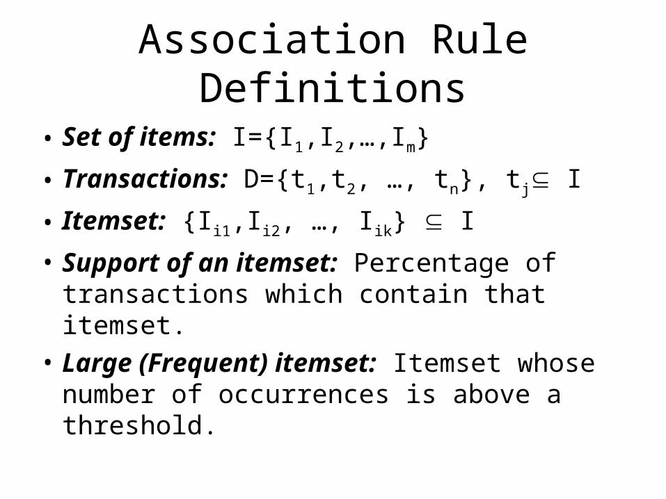
Association Rule Definitions

• Set of items: I={I1,I2,…,Im}

• Transactions: D={t1,t2, …, tn}, tj I

• Itemset: {Ii1,Ii2, …, Iik} I

• Support of an itemset: Percentage of transactions which contain that itemset.

• Large (Frequent) itemset: Itemset whose number of occurrences is above a threshold.

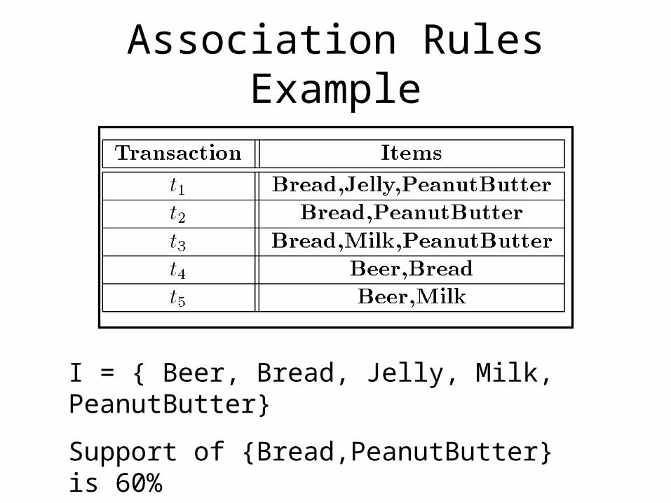
Association Rules Example

I = { Beer, Bread, Jelly, Milk, PeanutButter}

Support of {Bread,PeanutButter} is 60%

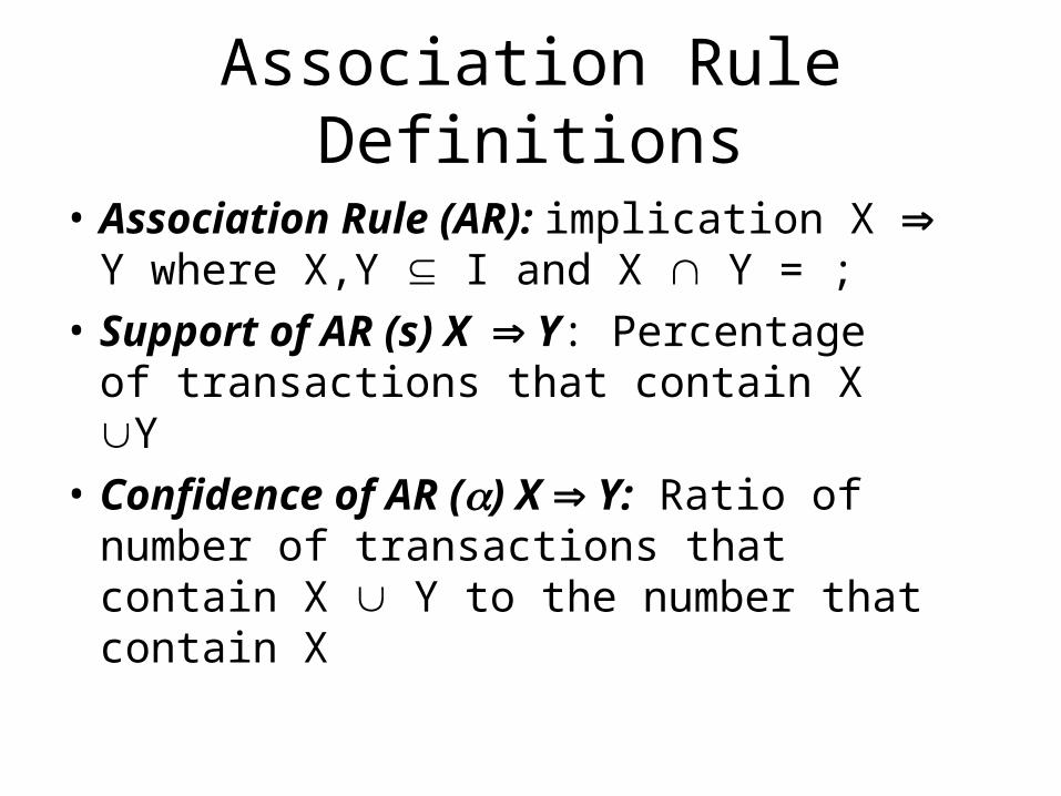
Association Rule Definitions

• Association Rule (AR): implication X Y where X,Y I and X Y = ;

• Support of AR (s) X Y: Percentage of transactions that contain X Y

• Confidence of AR () X Y: Ratio of number of transactions that contain X Y to the number that contain X

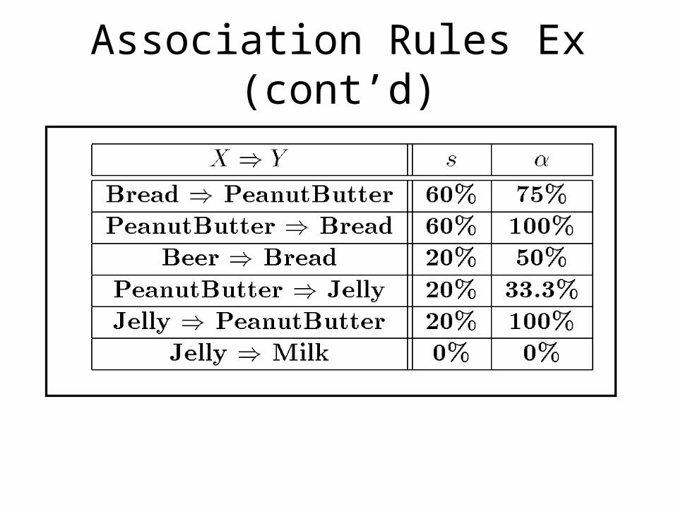
Association Rules Ex (cont’d)

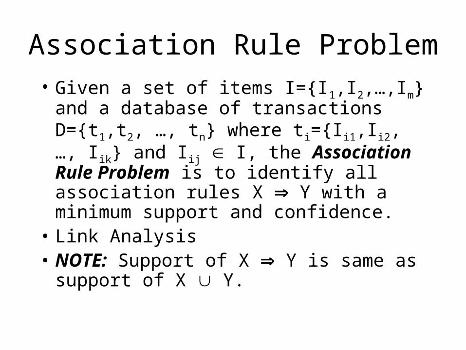
Association Rule Problem

• Given a set of items I={I1,I2,…,Im} and a database of transactions D={t1,t2, …, tn} where ti={Ii1,Ii2, …, Iik} and Iij I, the Association Rule Problem is to identify all association rules X Y with a minimum support and confidence.

• Link Analysis• NOTE: Support of X Y is same as

support of X Y.

Association Rule Techniques

1. Find Large Itemsets.

2. Generate rules from frequent itemsets.

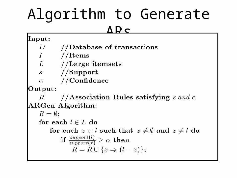
Algorithm to Generate ARs

Apriori

• Large Itemset Property:

Any subset of a large itemset is large.

• Contrapositive:

If an itemset is not large,

none of its supersets are large.

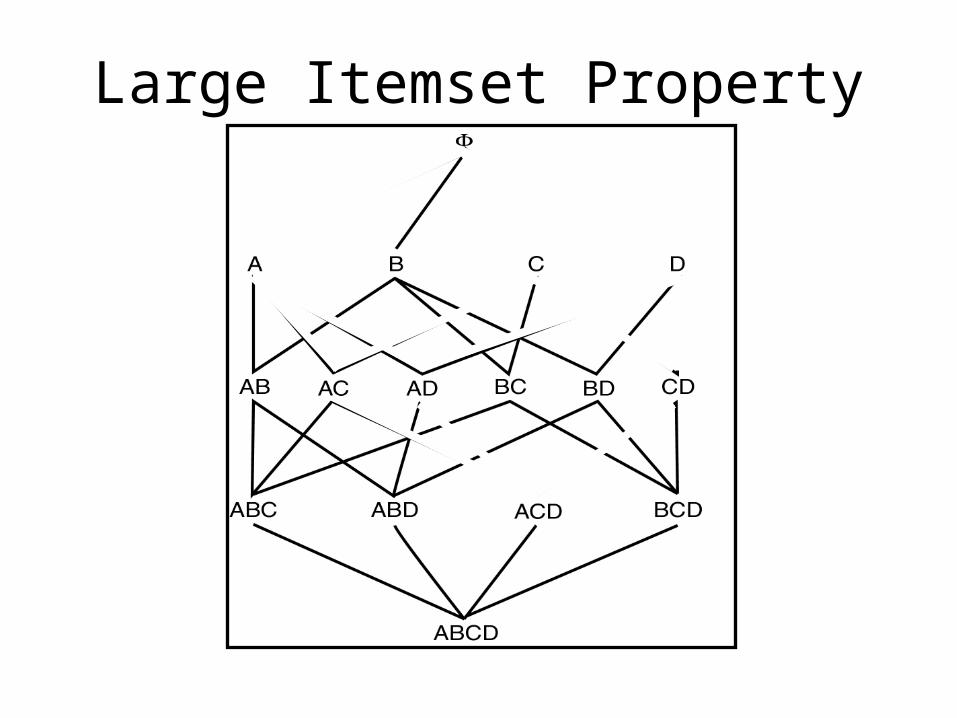
Large Itemset Property

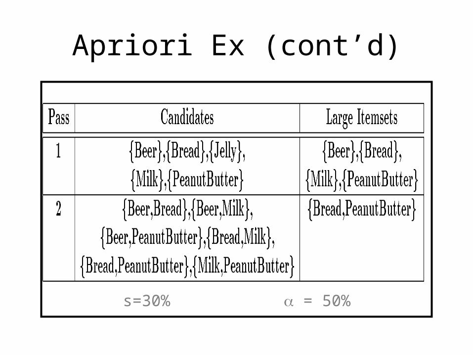
Apriori Ex (cont’d)

s=30% = 50%

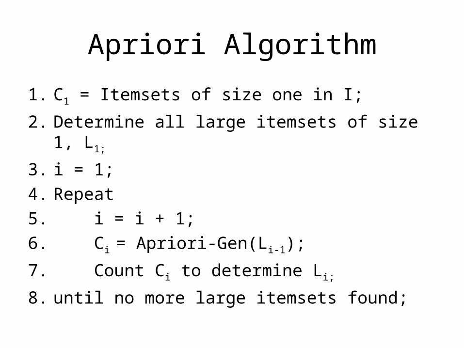
Apriori Algorithm

1. C1 = Itemsets of size one in I;

2. Determine all large itemsets of size 1, L1;

3. i = 1;

4. Repeat

5. i = i + 1;

6. Ci = Apriori-Gen(Li-1);

7. Count Ci to determine Li;

8. until no more large itemsets found;

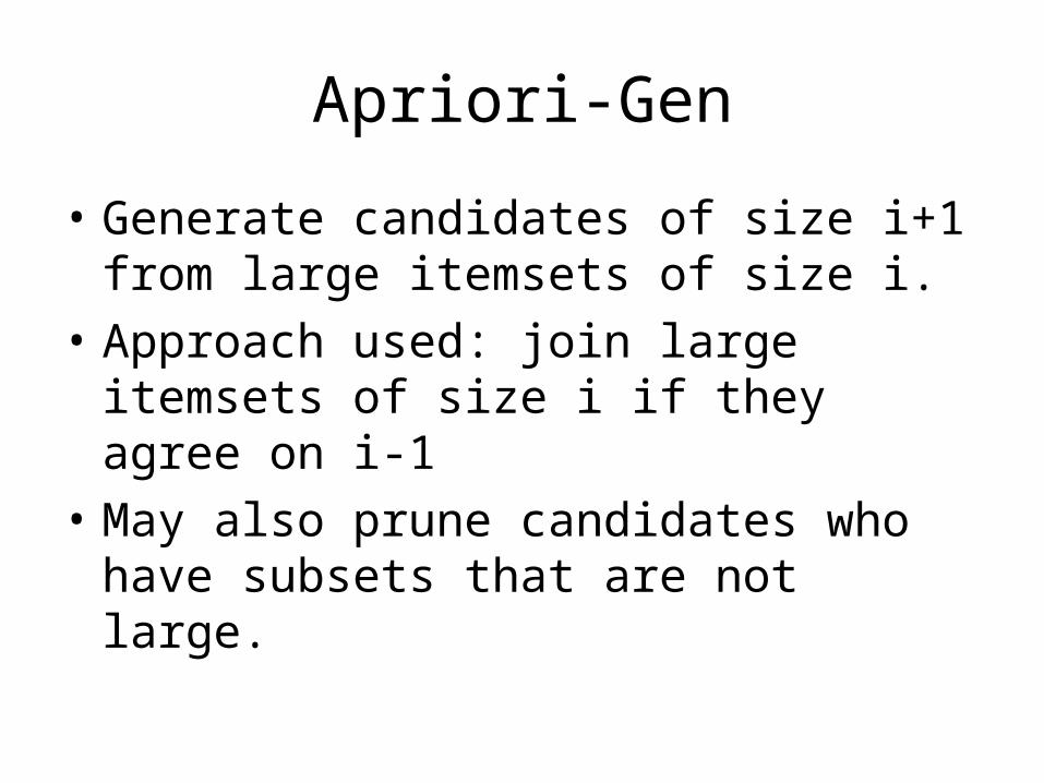
Apriori-Gen

• Generate candidates of size i+1 from large itemsets of size i.

• Approach used: join large itemsets of size i if they agree on i-1

• May also prune candidates who have subsets that are not large.

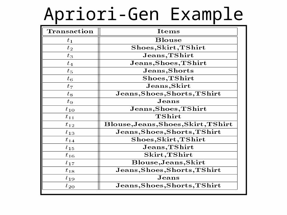
Apriori-Gen Example

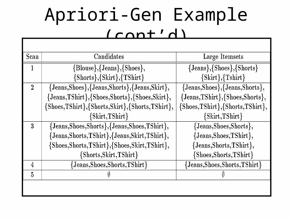
Apriori-Gen Example (cont’d)

Apriori Adv/Disadv

• Advantages:– Uses large itemset property.– Easily parallelized– Easy to implement.

• Disadvantages:– Assumes transaction database is memory

resident.– Requires up to m database scans.

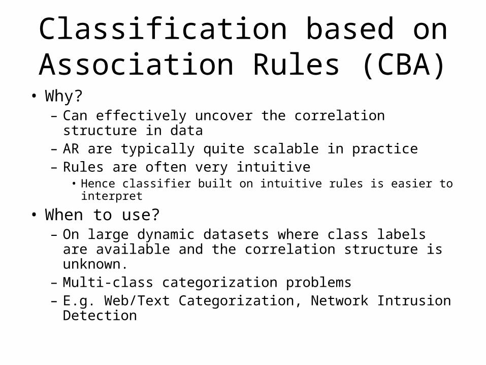
Classification based on Association Rules (CBA)

• Why?– Can effectively uncover the correlation structure in

data– AR are typically quite scalable in practice– Rules are often very intuitive

• Hence classifier built on intuitive rules is easier to interpret

• When to use?– On large dynamic datasets where class labels are

available and the correlation structure is unknown.– Multi-class categorization problems– E.g. Web/Text Categorization, Network Intrusion

Detection

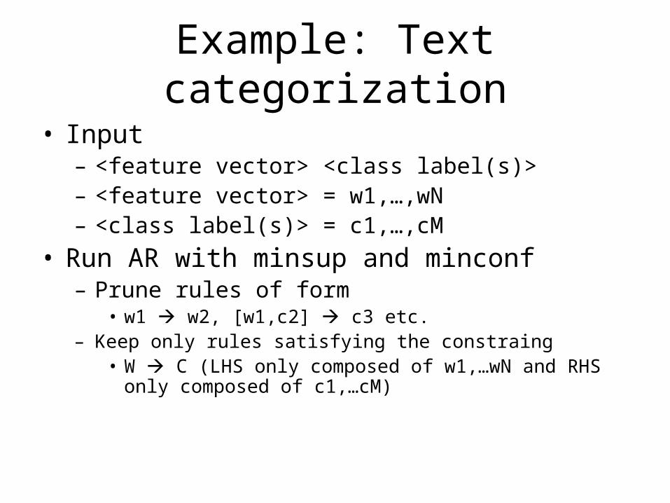
Example: Text categorization

• Input– <feature vector> <class label(s)>– <feature vector> = w1,…,wN– <class label(s)> = c1,…,cM

• Run AR with minsup and minconf– Prune rules of form

• w1 w2, [w1,c2] c3 etc.– Keep only rules satisfying the constraing

• W C (LHS only composed of w1,…wN and RHS only composed of c1,…cM)

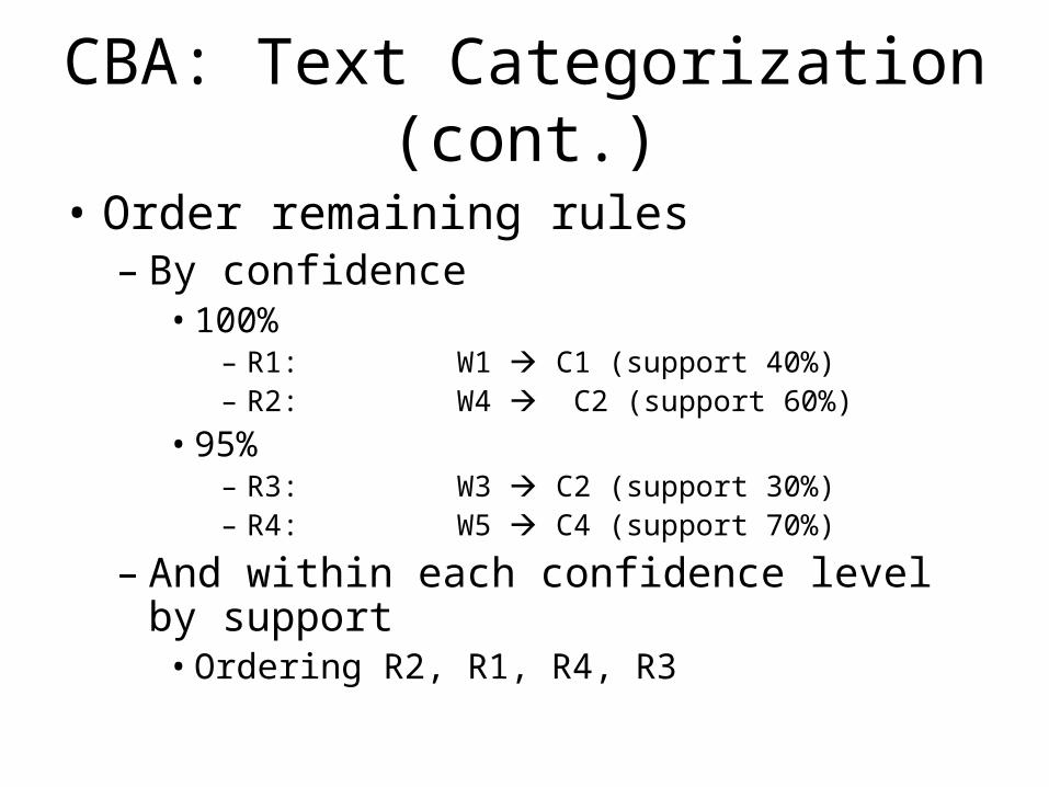
CBA: Text Categorization (cont.)

• Order remaining rules– By confidence

• 100%– R1: W1 C1 (support 40%)– R2: W4 C2 (support 60%)

• 95%– R3: W3 C2 (support 30%)– R4: W5 C4 (support 70%)

– And within each confidence level by support• Ordering R2, R1, R4, R3

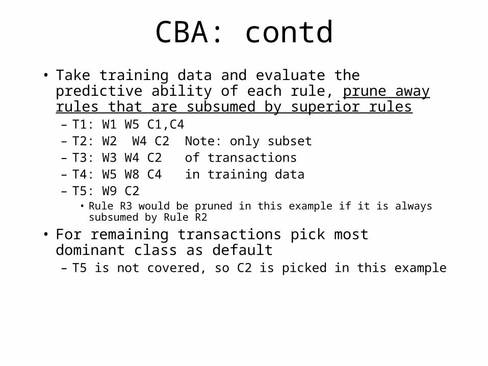
CBA: contd• Take training data and evaluate the predictive ability of

each rule, prune away rules that are subsumed by superior rules– T1: W1 W5 C1,C4– T2: W2 W4 C2 Note: only subset– T3: W3 W4 C2 of transactions– T4: W5 W8 C4 in training data– T5: W9 C2

• Rule R3 would be pruned in this example if it is always subsumed by Rule R2

• For remaining transactions pick most dominant class as default– T5 is not covered, so C2 is picked in this example

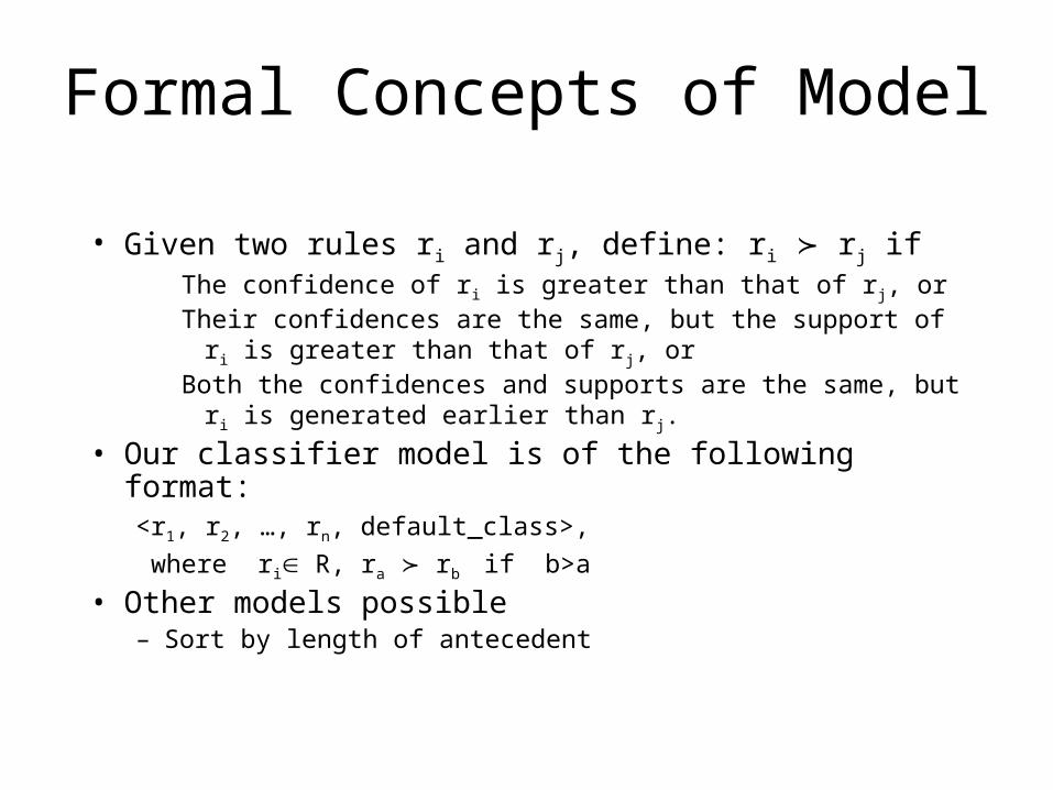
Formal Concepts of Model

• Given two rules ri and rj, define: ri rj ifThe confidence of ri is greater than that of rj, or

Their confidences are the same, but the support of ri is greater than that of rj, or

Both the confidences and supports are the same, but ri is generated earlier than rj.

• Our classifier model is of the following format:<r1, r2, …, rn, default_class>,

where ri R, ra rb if b>a

• Other models possible– Sort by length of antecedent

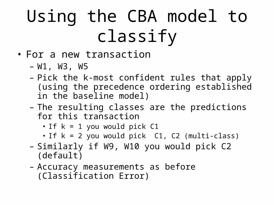
Using the CBA model to classify

• For a new transaction– W1, W3, W5– Pick the k-most confident rules that apply (using the

precedence ordering established in the baseline model)

– The resulting classes are the predictions for this transaction

• If k = 1 you would pick C1• If k = 2 you would pick C1, C2 (multi-class)

– Similarly if W9, W10 you would pick C2 (default)– Accuracy measurements as before (Classification

Error)

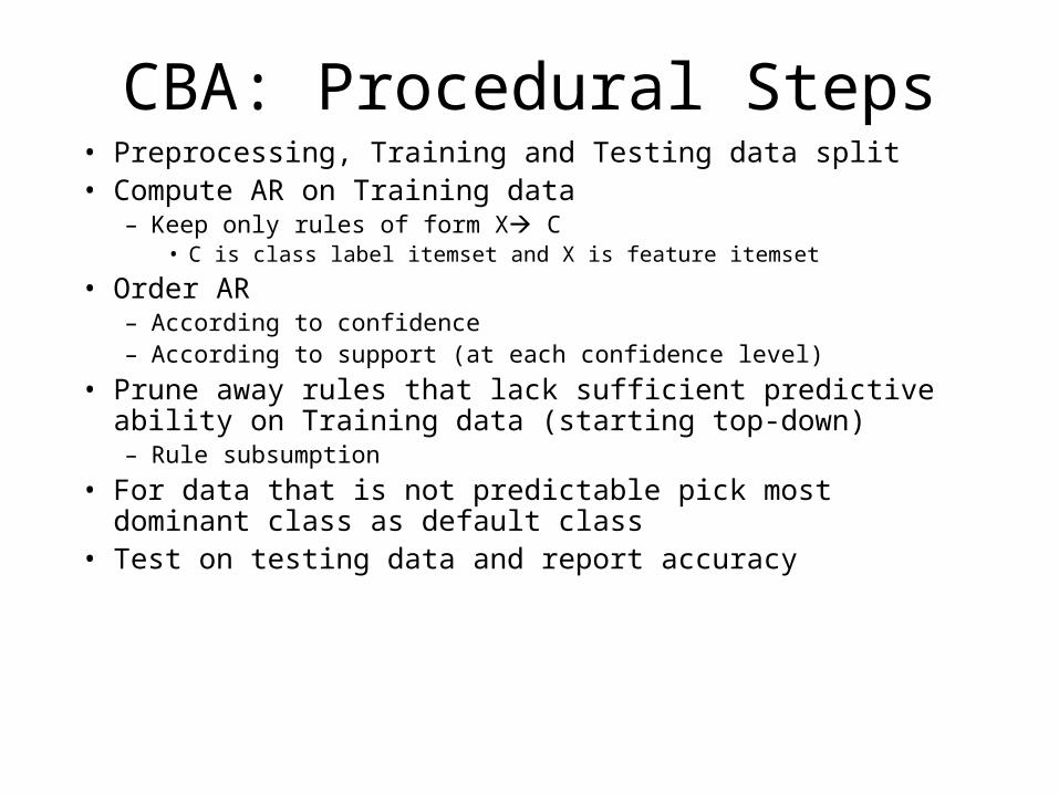
CBA: Procedural Steps• Preprocessing, Training and Testing data split• Compute AR on Training data

– Keep only rules of form X C• C is class label itemset and X is feature itemset

• Order AR– According to confidence– According to support (at each confidence level)

• Prune away rules that lack sufficient predictive ability on Training data (starting top-down)– Rule subsumption

• For data that is not predictable pick most dominant class as default class

• Test on testing data and report accuracy

Association Rules: Advanced Topics

Apriori Adv/Disadv

• Advantages:– Uses large itemset property.– Easily parallelized– Easy to implement.

• Disadvantages:– Assumes transaction database is memory

resident.– Requires up to m database scans.

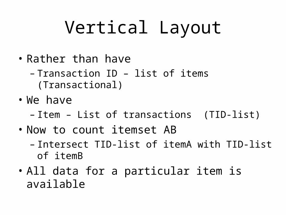
Vertical Layout

• Rather than have– Transaction ID – list of items (Transactional)

• We have– Item – List of transactions (TID-list)

• Now to count itemset AB– Intersect TID-list of itemA with TID-list of itemB

• All data for a particular item is available

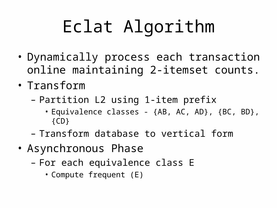
Eclat Algorithm

• Dynamically process each transaction online maintaining 2-itemset counts.

• Transform– Partition L2 using 1-item prefix

• Equivalence classes - {AB, AC, AD}, {BC, BD}, {CD}

– Transform database to vertical form

• Asynchronous Phase– For each equivalence class E

• Compute frequent (E)

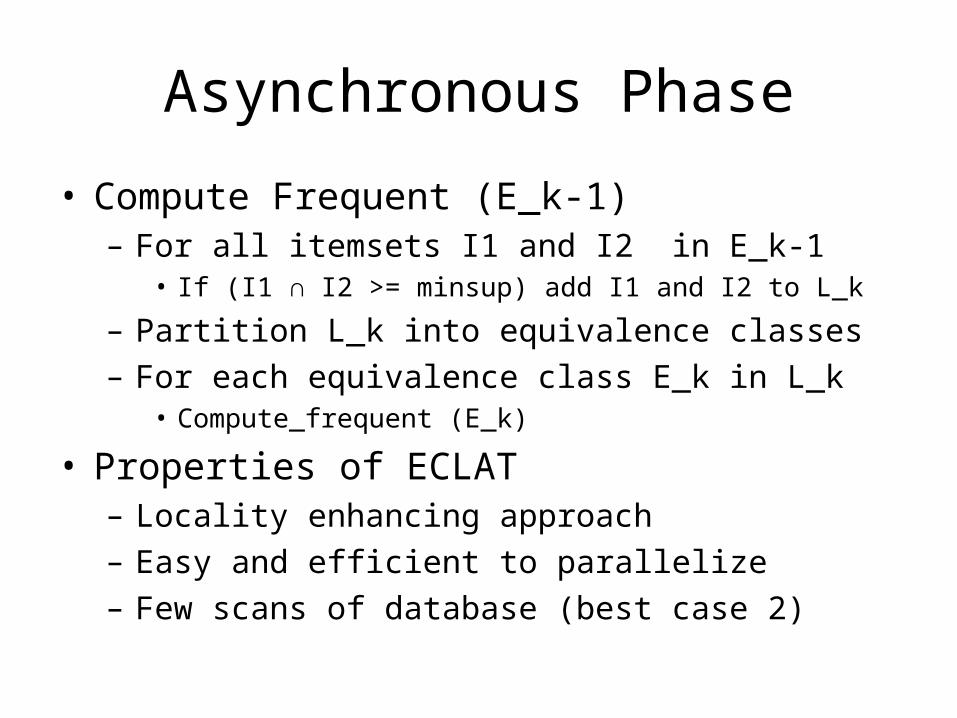
Asynchronous Phase

• Compute Frequent (E_k-1)– For all itemsets I1 and I2 in E_k-1

• If (I1 ∩ I2 >= minsup) add I1 and I2 to L_k

– Partition L_k into equivalence classes– For each equivalence class E_k in L_k

• Compute_frequent (E_k)

• Properties of ECLAT– Locality enhancing approach– Easy and efficient to parallelize– Few scans of database (best case 2)

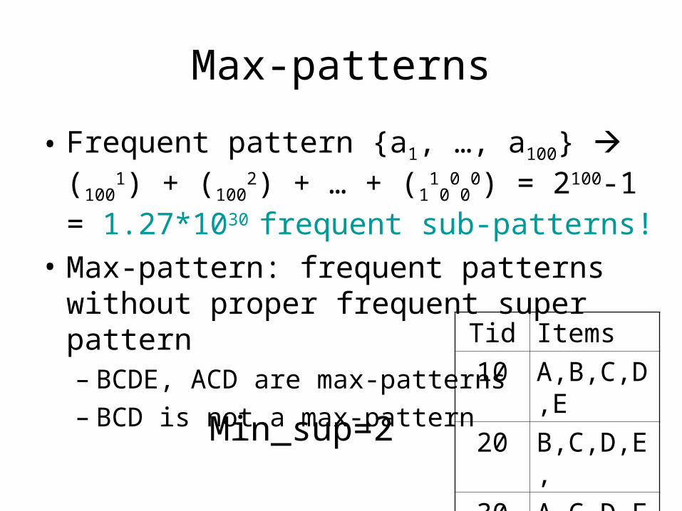
Max-patterns

• Frequent pattern {a1, …, a100} (1001) + (100

2) + … + (1

10

00

0) = 2100-1 = 1.27*1030 frequent sub-patterns!

• Max-pattern: frequent patterns without proper frequent super pattern– BCDE, ACD are max-patterns– BCD is not a max-pattern

Tid Items

10 A,B,C,D,E

20 B,C,D,E,

30 A,C,D,F

Min_sup=2

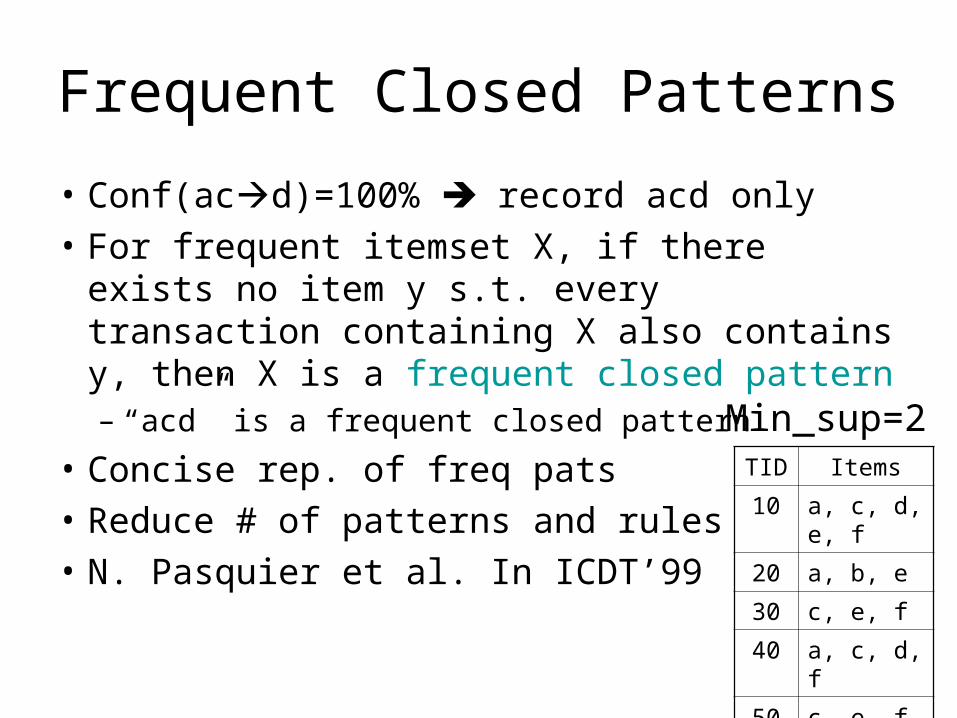
Frequent Closed Patterns

• Conf(acd)=100% record acd only• For frequent itemset X, if there exists no item

y s.t. every transaction containing X also contains y, then X is a frequent closed pattern– “acd” is a frequent closed pattern

• Concise rep. of freq pats• Reduce # of patterns and rules• N. Pasquier et al. In ICDT’99

TID Items

10 a, c, d, e, f

20 a, b, e

30 c, e, f

40 a, c, d, f

50 c, e, f

Min_sup=2

Mining Various Kinds of Rules or Regularities

• Multi-level, quantitative association rules,

correlation and causality, ratio rules,

sequential patterns, emerging patterns,

temporal associations, partial periodicity

• Classification, clustering, iceberg cubes, etc.

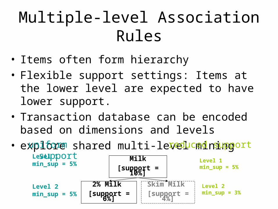
Multiple-level Association Rules

• Items often form hierarchy• Flexible support settings: Items at the lower level

are expected to have lower support.• Transaction database can be encoded based on

dimensions and levels• explore shared multi-level mining

uniform support

Milk[support = 10%]

2% Milk [support = 6%]

Skim Milk [support = 4%]

Level 1min_sup = 5%

Level 2min_sup = 5%

Level 1min_sup = 5%

Level 2min_sup = 3%

reduced support

ML/MD Associations with Flexible Support Constraints

• Why flexible support constraints?– Real life occurrence frequencies vary greatly

• Diamond, watch, pens in a shopping basket

– Uniform support may not be an interesting model

• A flexible model– The lower-level, the more dimension combination, and the long

pattern length, usually the smaller support

– General rules should be easy to specify and understand

– Special items and special group of items may be specified individually and have higher priority

Multi-dimensional Association

• Single-dimensional rules:

buys(X, “milk”) buys(X, “bread”)

• Multi-dimensional rules: 2 dimensions or predicates

– Inter-dimension assoc. rules (no repeated predicates)

age(X,”19-25”) occupation(X,“student”)

buys(X,“coke”)

– hybrid-dimension assoc. rules (repeated predicates)

age(X,”19-25”) buys(X, “popcorn”) buys(X,

“coke”)

Multi-level Association: Redundancy Filtering

• Some rules may be redundant due to “ancestor”

relationships between items.

• Example– milk wheat bread [support = 8%, confidence = 70%]

– 2% milk wheat bread [support = 2%, confidence = 72%]

• We say the first rule is an ancestor of the second

rule.

• A rule is redundant if its support is close to the

“expected” value, based on the rule’s ancestor.

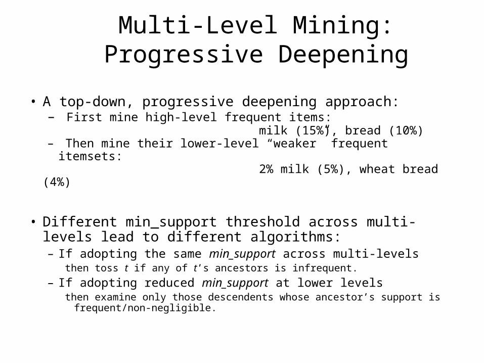
Multi-Level Mining: Progressive Deepening

• A top-down, progressive deepening approach:– First mine high-level frequent items:

milk (15%), bread (10%)– Then mine their lower-level “weaker” frequent itemsets:

2% milk (5%), wheat bread (4%)

• Different min_support threshold across multi-levels lead to different algorithms:– If adopting the same min_support across multi-levels

then toss t if any of t’s ancestors is infrequent.

– If adopting reduced min_support at lower levelsthen examine only those descendents whose ancestor’s support is

frequent/non-negligible.

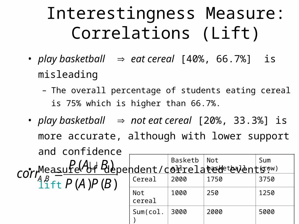
Interestingness Measure: Correlations (Lift)

• play basketball eat cereal [40%, 66.7%] is misleading

– The overall percentage of students eating cereal is 75% which is

higher than 66.7%.

• play basketball not eat cereal [20%, 33.3%] is more

accurate, although with lower support and confidence

• Measure of dependent/correlated events: lift

Basketball

Not basketball Sum (row)

Cereal 2000 1750 3750

Not cereal 1000 250 1250

Sum(col.) 3000 2000 5000

)()(

)(, BPAP

BAPcorr BA

Constraint-based Data Mining

• Finding all the patterns in a database autonomously? — unrealistic!– The patterns could be too many but not focused!

• Data mining should be an interactive process – User directs what to be mined using a data mining

query language (or a graphical user interface)

• Constraint-based mining– User flexibility: provides constraints on what to be

mined– System optimization: explores such constraints for

efficient mining—constraint-based mining

Constrained Frequent Pattern Mining: A Mining Query Optimization Problem

• Given a frequent pattern mining query with a set of constraints C, the algorithm should be– sound: it only finds frequent sets that satisfy the given

constraints C– complete: all frequent sets satisfying the given

constraints C are found• A naïve solution

– First find all frequent sets, and then test them for constraint satisfaction

• More efficient approaches:– Analyze the properties of constraints comprehensively – Push them as deeply as possible inside the frequent

pattern computation.

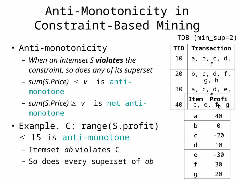
Anti-Monotonicity in Constraint-Based Mining

• Anti-monotonicity– When an intemset S violates the

constraint, so does any of its superset

– sum(S.Price) v is anti-monotone

– sum(S.Price) v is not anti-monotone

• Example. C: range(S.profit) 15 is anti-monotone– Itemset ab violates C

– So does every superset of ab

TID Transaction

10 a, b, c, d, f

20 b, c, d, f, g, h

30 a, c, d, e, f

40 c, e, f, g

TDB (min_sup=2)

Item Profit

a 40

b 0

c -20

d 10

e -30

f 30

g 20

h -10

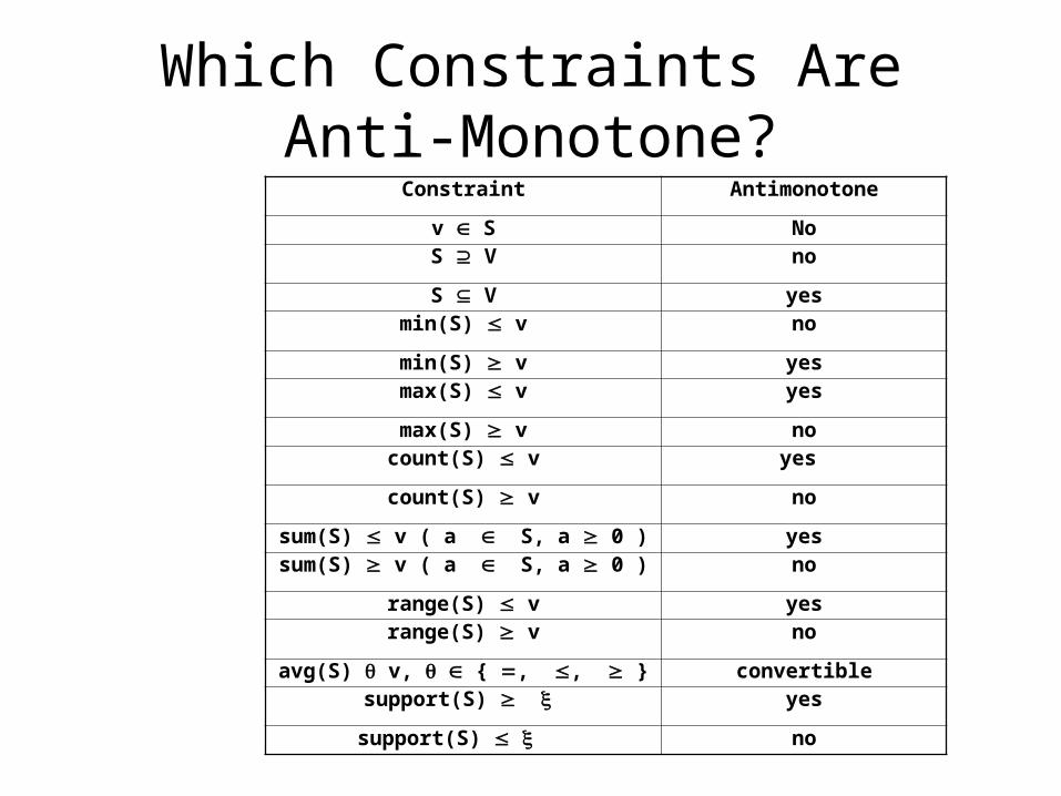
Which Constraints Are Anti-Monotone?

Constraint Antimonotone

v S NoS V no

S V yesmin(S) v no

min(S) v yesmax(S) v yes

max(S) v nocount(S) v yes

count(S) v no

sum(S) v ( a S, a 0 ) yessum(S) v ( a S, a 0 ) no

range(S) v yesrange(S) v no

avg(S) v, { , , } convertiblesupport(S) yes

support(S) no

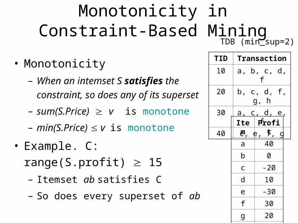
Monotonicity in Constraint-Based Mining

• Monotonicity

– When an intemset S satisfies the

constraint, so does any of its

superset

– sum(S.Price) v is monotone

– min(S.Price) v is monotone

• Example. C: range(S.profit) 15

– Itemset ab satisfies C

– So does every superset of ab

TID Transaction

10 a, b, c, d, f

20 b, c, d, f, g, h

30 a, c, d, e, f

40 c, e, f, g

TDB (min_sup=2)

Item Profit

a 40

b 0

c -20

d 10

e -30

f 30

g 20

h -10

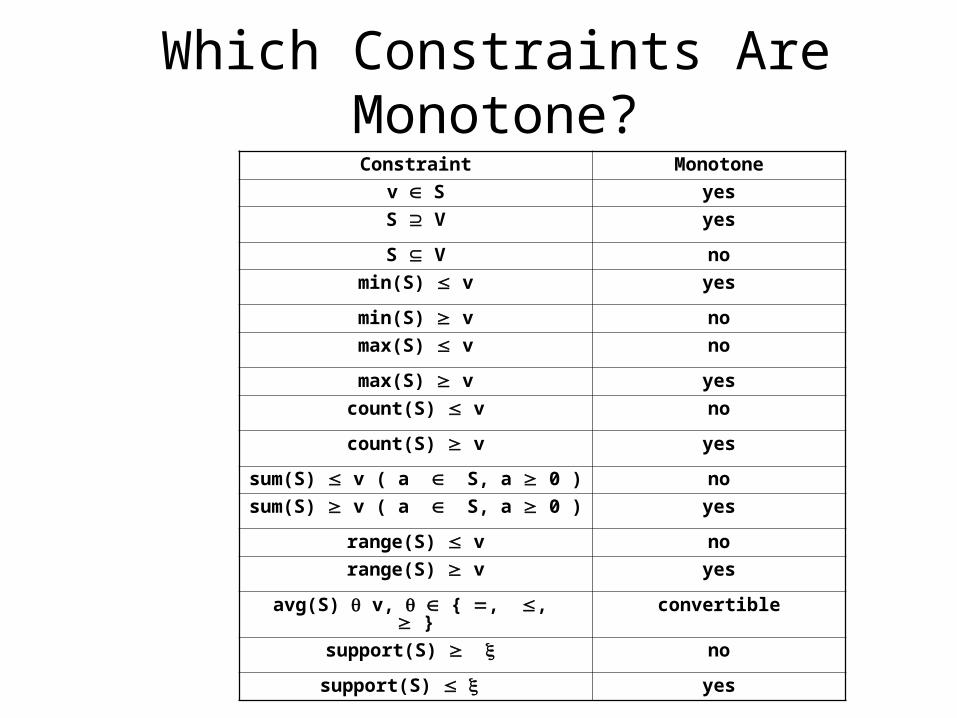
Which Constraints Are Monotone?Constraint Monotone

v S yes

S V yes

S V no

min(S) v yes

min(S) v no

max(S) v no

max(S) v yes

count(S) v no

count(S) v yes

sum(S) v ( a S, a 0 ) no

sum(S) v ( a S, a 0 ) yes

range(S) v no

range(S) v yes

avg(S) v, { , , } convertible

support(S) no

support(S) yes

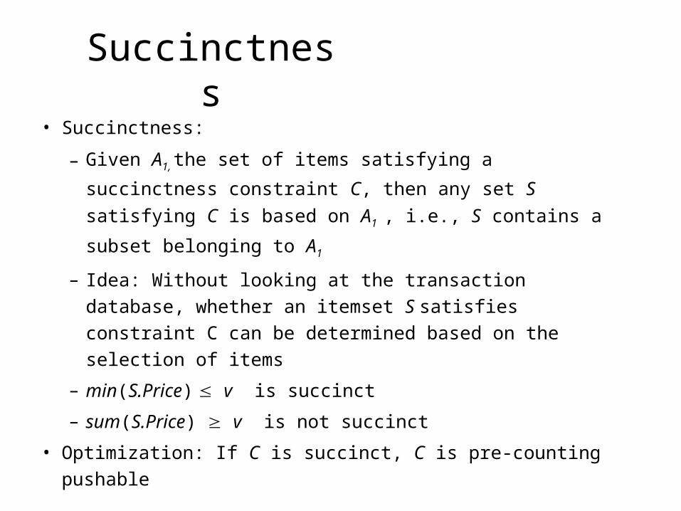
Succinctness

• Succinctness:

– Given A1, the set of items satisfying a succinctness

constraint C, then any set S satisfying C is based on

A1 , i.e., S contains a subset belonging to A1

– Idea: Without looking at the transaction database,

whether an itemset S satisfies constraint C can be

determined based on the selection of items

– min(S.Price) v is succinct

– sum(S.Price) v is not succinct

• Optimization: If C is succinct, C is pre-counting pushable

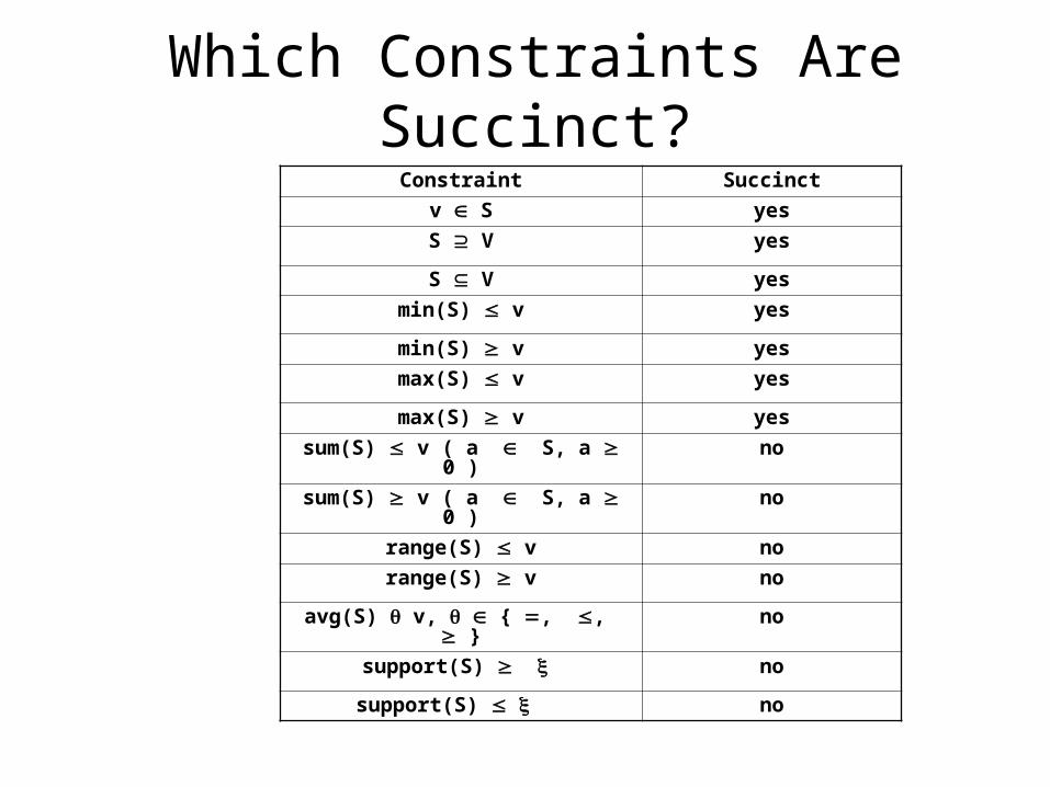
Which Constraints Are Succinct?Constraint Succinct

v S yes

S V yes

S V yes

min(S) v yes

min(S) v yes

max(S) v yes

max(S) v yes



range(S) v no

range(S) v no

avg(S) v, { , , } no

support(S) no

support(S) no

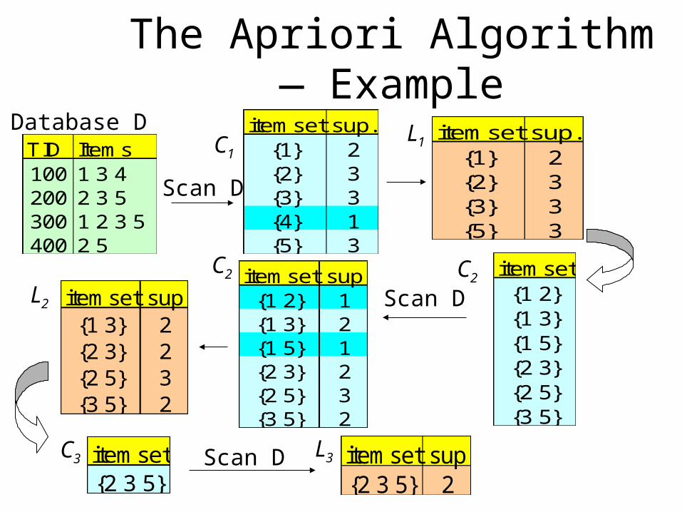
The Apriori Algorithm — Example

TID Items100 1 3 4200 2 3 5300 1 2 3 5400 2 5

Database D itemset sup.{1} 2{2} 3{3} 3{4} 1{5} 3

itemset sup.{1} 2{2} 3{3} 3{5} 3

Scan D

C1L1

itemset{1 2}{1 3}{1 5}{2 3}{2 5}{3 5}

itemset sup{1 2} 1{1 3} 2{1 5} 1{2 3} 2{2 5} 3{3 5} 2

itemset sup{1 3} 2{2 3} 2{2 5} 3{3 5} 2

L2

C2 C2Scan D

C3 L3itemset{2 3 5}

Scan D itemset sup{2 3 5} 2

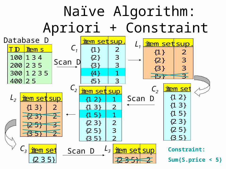
Naïve Algorithm: Apriori + Constraint

TID Items100 1 3 4200 2 3 5300 1 2 3 5400 2 5


itemset sup.{1} 2{2} 3{3} 3{5} 3

Scan D

C1L1

itemset{1 2}{1 3}{1 5}{2 3}{2 5}{3 5}

itemset sup{1 2} 1{1 3} 2{1 5} 1{2 3} 2{2 5} 3{3 5} 2

itemset sup{1 3} 2{2 3} 2{2 5} 3{3 5} 2

L2

C2 C2Scan D

C3 L3itemset{2 3 5}


Constraint:

Sum{S.price < 5}

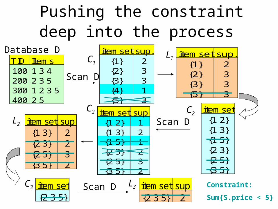
Pushing the constraint deep into the process

TID Items100 1 3 4200 2 3 5300 1 2 3 5400 2 5


itemset sup.{1} 2{2} 3{3} 3{5} 3

Scan D

C1L1

itemset{1 2}{1 3}{1 5}{2 3}{2 5}{3 5}

itemset sup{1 2} 1{1 3} 2{1 5} 1{2 3} 2{2 5} 3{3 5} 2

itemset sup{1 3} 2{2 3} 2{2 5} 3{3 5} 2

L2

C2 C2Scan D

C3 L3itemset{2 3 5}


Constraint:

Sum{S.price < 5}

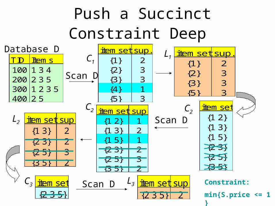
Push a Succinct Constraint Deep

TID Items100 1 3 4200 2 3 5300 1 2 3 5400 2 5


itemset sup.{1} 2{2} 3{3} 3{5} 3

Scan D

C1L1

itemset{1 2}{1 3}{1 5}{2 3}{2 5}{3 5}

itemset sup{1 2} 1{1 3} 2{1 5} 1{2 3} 2{2 5} 3{3 5} 2

itemset sup{1 3} 2{2 3} 2{2 5} 3{3 5} 2

L2

C2 C2Scan D

C3 L3itemset{2 3 5}


Constraint:

min{S.price <= 1 }

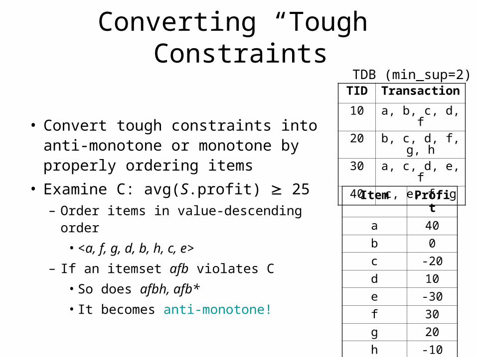
Converting “Tough” Constraints

• Convert tough constraints into anti-monotone or monotone by properly ordering items

• Examine C: avg(S.profit) 25– Order items in value-descending order

• <a, f, g, d, b, h, c, e>

– If an itemset afb violates C

• So does afbh, afb*

• It becomes anti-monotone!

TID Transaction

10 a, b, c, d, f

20 b, c, d, f, g, h

30 a, c, d, e, f

40 c, e, f, g

TDB (min_sup=2)

Item Profit

a 40

b 0

c -20

d 10

e -30

f 30

g 20

h -10

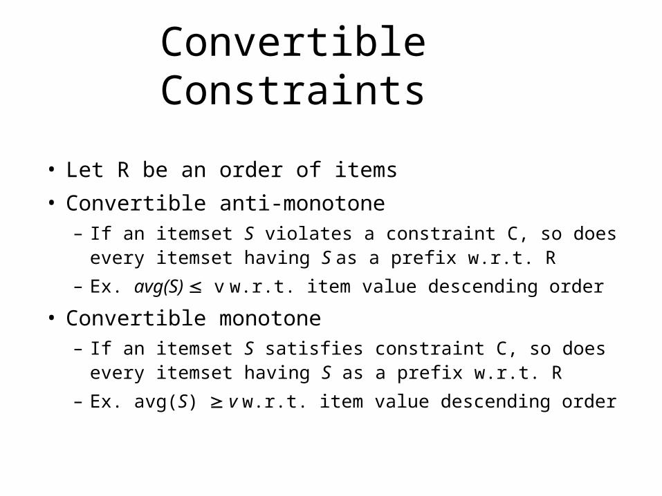
Convertible Constraints

• Let R be an order of items

• Convertible anti-monotone– If an itemset S violates a constraint C, so does every

itemset having S as a prefix w.r.t. R

– Ex. avg(S) v w.r.t. item value descending order

• Convertible monotone– If an itemset S satisfies constraint C, so does every

itemset having S as a prefix w.r.t. R

– Ex. avg(S) v w.r.t. item value descending order

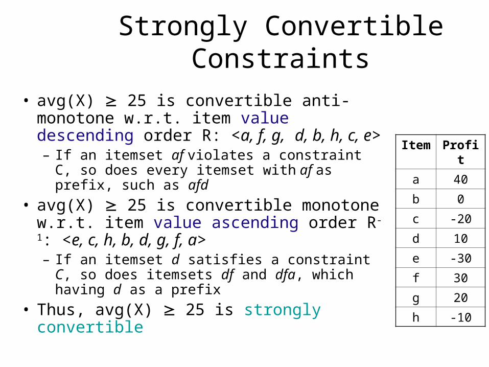
Strongly Convertible Constraints

• avg(X) 25 is convertible anti-monotone w.r.t. item value descending order R: <a, f, g, d, b, h, c, e>– If an itemset af violates a constraint C, so does

every itemset with af as prefix, such as afd

• avg(X) 25 is convertible monotone w.r.t. item value ascending order R-1: <e, c, h, b, d, g, f, a>– If an itemset d satisfies a constraint C, so does

itemsets df and dfa, which having d as a prefix

• Thus, avg(X) 25 is strongly convertible

Item Profit

a 40

b 0

c -20

d 10

e -30

f 30

g 20

h -10

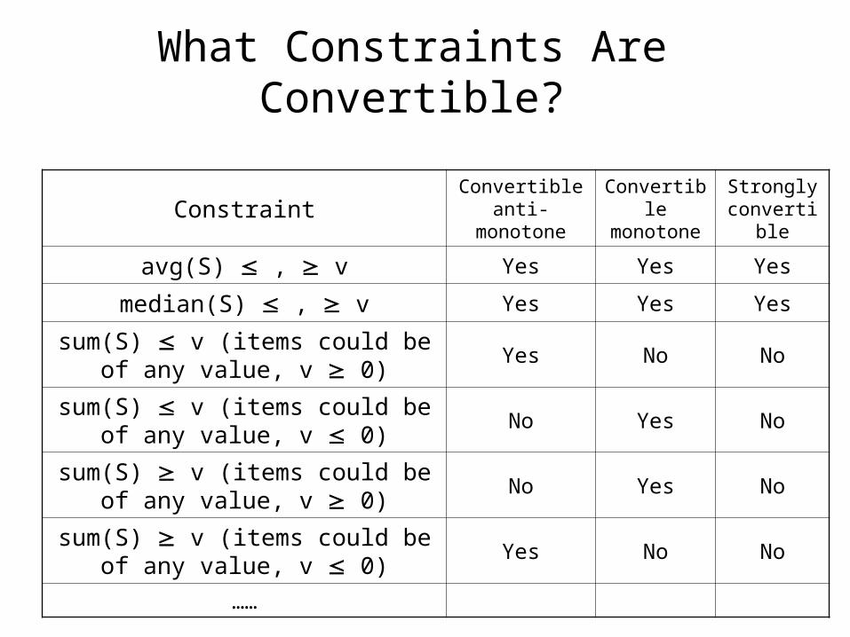
What Constraints Are Convertible?

ConstraintConvertible

anti-monotoneConvertible monotone

Strongly convertible

avg(S) , v Yes Yes Yes

median(S) , v Yes Yes Yes

sum(S) v (items could be of any value, v 0)

Yes No No


No Yes No


No Yes No


Yes No No

……

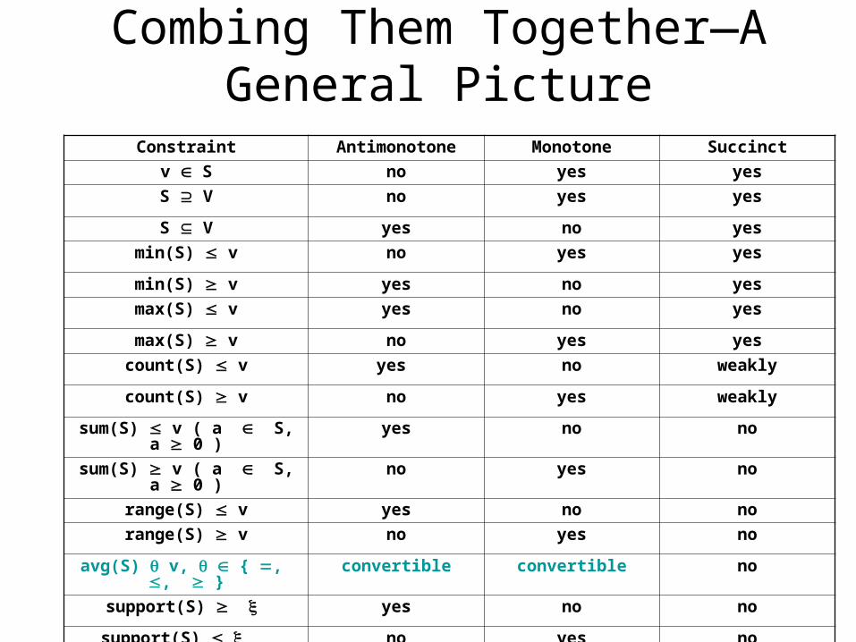
Combing Them Together—A General Picture

Constraint Antimonotone Monotone Succinct

v S no yes yes

S V no yes yes

S V yes no yes

min(S) v no yes yes

min(S) v yes no yes

max(S) v yes no yes

max(S) v no yes yes

count(S) v yes no weakly

count(S) v no yes weakly

sum(S) v ( a S, a 0 ) yes no no

sum(S) v ( a S, a 0 ) no yes no

range(S) v yes no no

range(S) v no yes no

avg(S) v, { , , } convertible convertible no

support(S) yes no no

support(S) no yes no

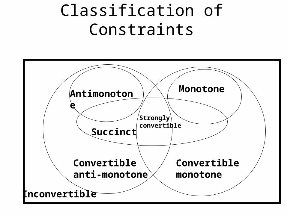
Classification of Constraints

Convertibleanti-monotone

Convertiblemonotone

Stronglyconvertible

Inconvertible

Succinct

Antimonotone

Monotone

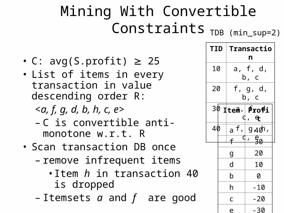
Mining With Convertible Constraints

• C: avg(S.profit) 25• List of items in every transaction

in value descending order R: <a, f, g, d, b, h, c, e>– C is convertible anti-monotone

w.r.t. R• Scan transaction DB once

– remove infrequent items• Item h in transaction 40 is

dropped– Itemsets a and f are good

TID Transaction

10 a, f, d, b, c

20 f, g, d, b, c

30 a, f, d, c, e

40 f, g, h, c, e

TDB (min_sup=2)

Item Profit

a 40

f 30

g 20

d 10

b 0

h -10

c -20

e -30

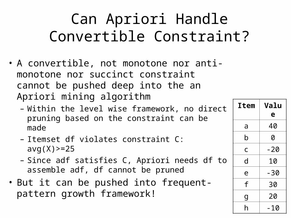
Can Apriori Handle Convertible Constraint?

• A convertible, not monotone nor anti-monotone nor succinct constraint cannot be pushed deep into the an Apriori mining algorithm– Within the level wise framework, no direct

pruning based on the constraint can be made

– Itemset df violates constraint C: avg(X)>=25

– Since adf satisfies C, Apriori needs df to assemble adf, df cannot be pruned

• But it can be pushed into frequent-pattern growth framework!

Item Value

a 40

b 0

c -20

d 10

e -30

f 30

g 20

h -10

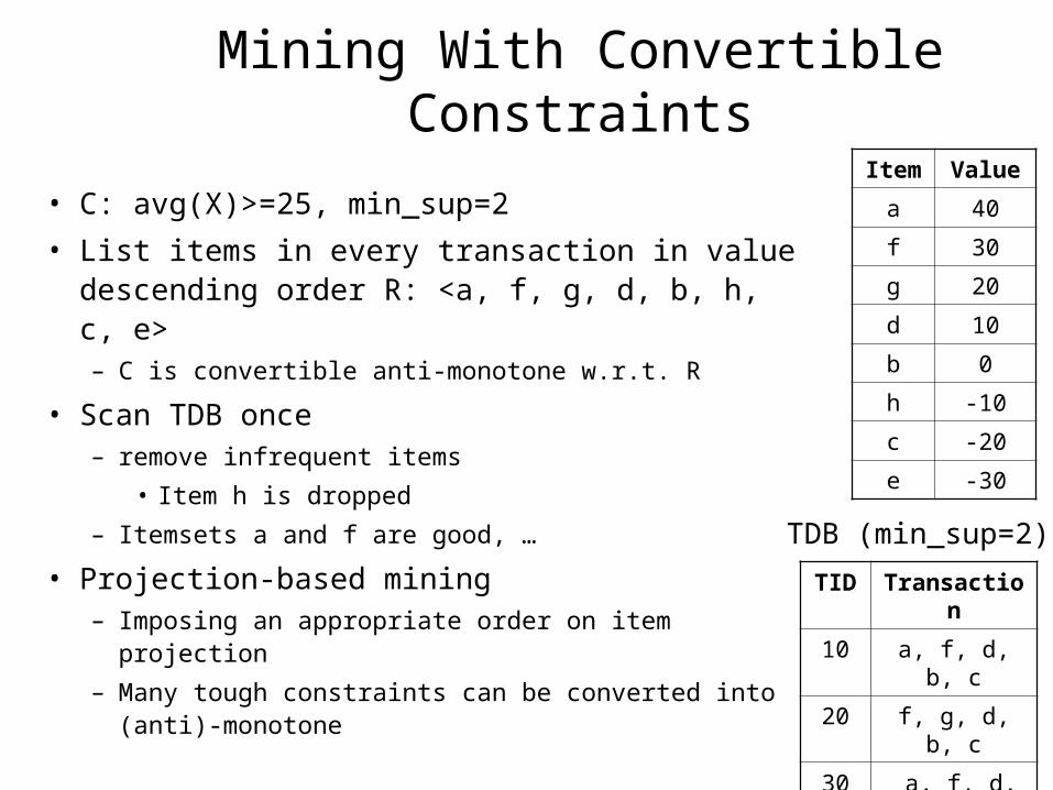
Mining With Convertible Constraints

• C: avg(X)>=25, min_sup=2

• List items in every transaction in value descending order R: <a, f, g, d, b, h, c, e>– C is convertible anti-monotone w.r.t. R

• Scan TDB once– remove infrequent items

• Item h is dropped

– Itemsets a and f are good, …

• Projection-based mining– Imposing an appropriate order on item projection

– Many tough constraints can be converted into (anti)-monotone

TID Transaction

10 a, f, d, b, c

20 f, g, d, b, c

30 a, f, d, c, e

40 f, g, h, c, e

TDB (min_sup=2)

Item Value

a 40

f 30

g 20

d 10

b 0

h -10

c -20

e -30

Handling Multiple Constraints

• Different constraints may require different or even

conflicting item-ordering

• If there exists an order R s.t. both C1 and C2 are

convertible w.r.t. R, then there is no conflict between

the two convertible constraints

• If there exists conflict on order of items

– Try to satisfy one constraint first

– Then using the order for the other constraint to mine

frequent itemsets in the corresponding projected database

Sequence Mining

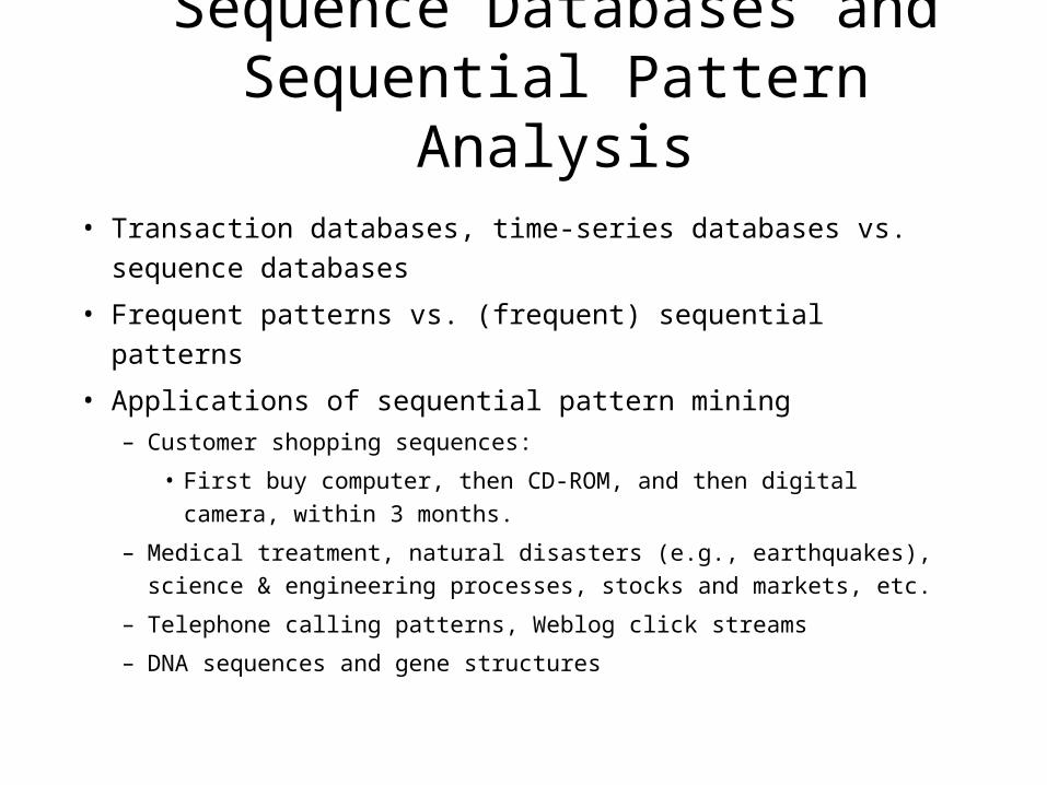
Sequence Databases and Sequential Pattern Analysis

• Transaction databases, time-series databases vs. sequence

databases

• Frequent patterns vs. (frequent) sequential patterns

• Applications of sequential pattern mining

– Customer shopping sequences:

• First buy computer, then CD-ROM, and then digital camera, within

3 months.

– Medical treatment, natural disasters (e.g., earthquakes), science &

engineering processes, stocks and markets, etc.

– Telephone calling patterns, Weblog click streams

– DNA sequences and gene structures

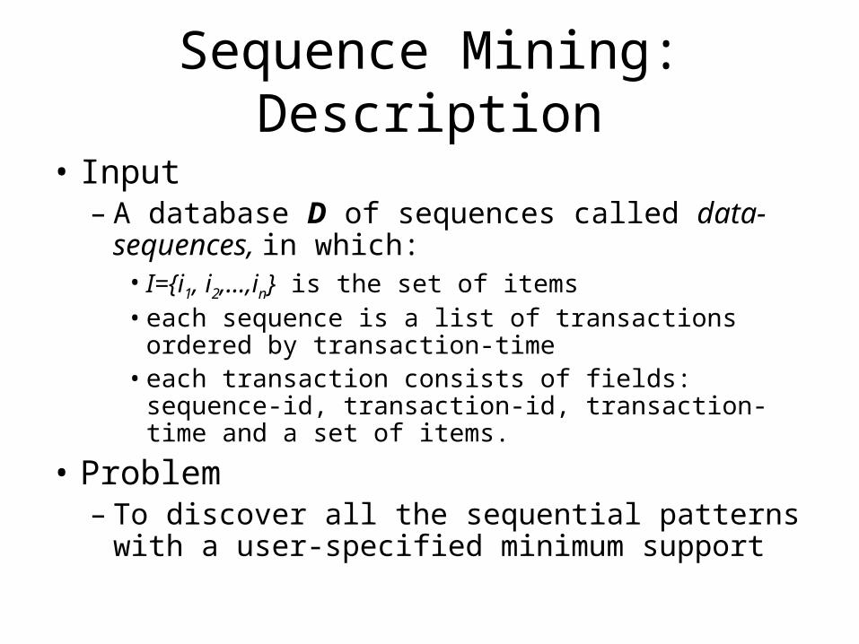
Sequence Mining: Description

• Input– A database D of sequences called data-

sequences, in which:• I={i1, i2,…,in} is the set of items• each sequence is a list of transactions ordered by

transaction-time • each transaction consists of fields: sequence-id,

transaction-id, transaction-time and a set of items.

• Problem– To discover all the sequential patterns with a

user-specified minimum support

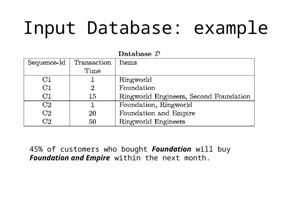
Input Database: example

45% of customers who bought Foundation will buy Foundation and Empire within the next month.

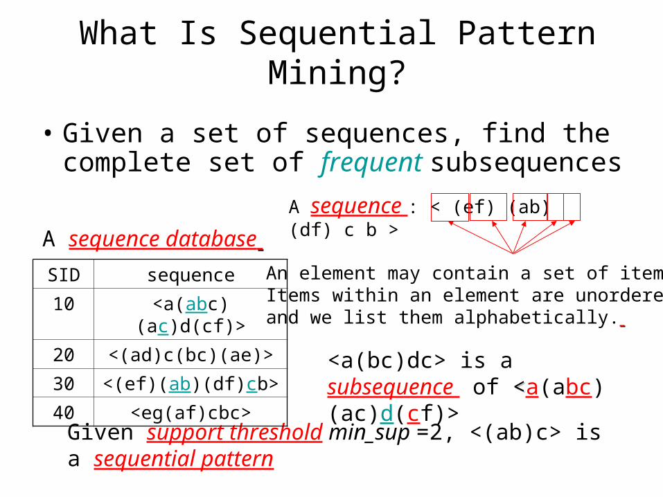
What Is Sequential Pattern Mining?

• Given a set of sequences, find the complete set of frequent subsequences

A sequence database

A sequence : < (ef) (ab) (df) c b >

An element may contain a set of items.Items within an element are unorderedand we list them alphabetically.

<a(bc)dc> is a subsequence of <<a(abc)(ac)d(cf)>

Given support threshold min_sup =2, <(ab)c> is a sequential pattern

SID sequence

10 <a(abc)(ac)d(cf)>

20 <(ad)c(bc)(ae)>

30 <(ef)(ab)(df)cb>

40 <eg(af)cbc>

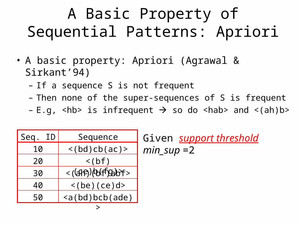
A Basic Property of Sequential Patterns: Apriori

• A basic property: Apriori (Agrawal & Sirkant’94) – If a sequence S is not frequent – Then none of the super-sequences of S is frequent– E.g, <hb> is infrequent so do <hab> and <(ah)b>

<a(bd)bcb(ade)>50

<(be)(ce)d>40

<(ah)(bf)abf>30

<(bf)(ce)b(fg)>20

<(bd)cb(ac)>10

SequenceSeq. ID Given support threshold min_sup =2

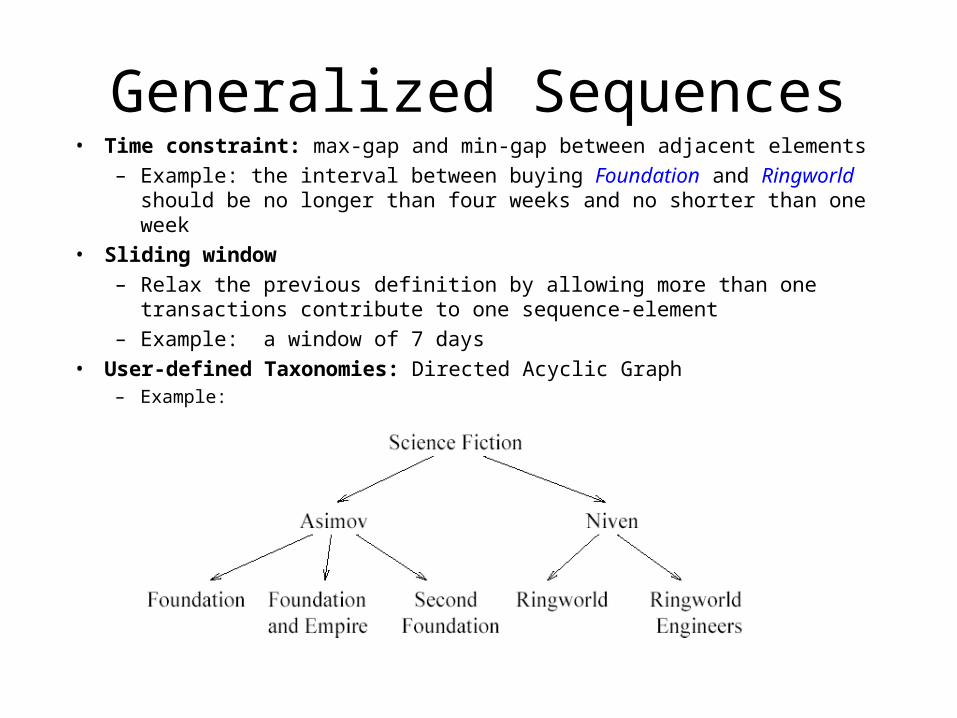
Generalized Sequences• Time constraint: max-gap and min-gap between adjacent elements

– Example: the interval between buying Foundation and Ringworld should be no longer than four weeks and no shorter than one week

• Sliding window

– Relax the previous definition by allowing more than one transactions contribute to one sequence-element

– Example: a window of 7 days

• User-defined Taxonomies: Directed Acyclic Graph– Example:

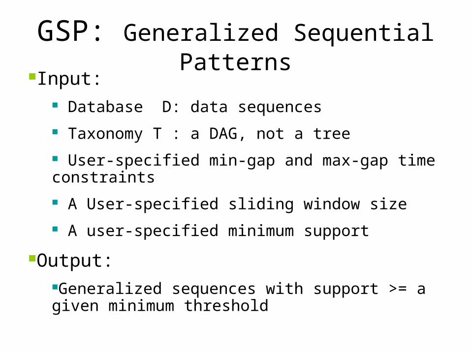
GSP: Generalized Sequential Patterns

Input: Database D: data sequences

Taxonomy T : a DAG, not a tree

User-specified min-gap and max-gap time constraints

A User-specified sliding window size

A user-specified minimum support

Output:Generalized sequences with support >= a given minimum threshold

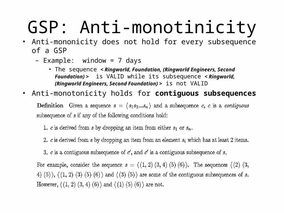
GSP: Anti-monotinicity• Anti-mononicity does not hold for every subsequence of a GSP

– Example: window = 7 days• The sequence < Ringworld, Foundation, (Ringworld Engineers, Second

Foundation) > is VALID while its subsequence < Ringworld, (Ringworld Engineers, Second Foundation) > is not VALID

• Anti-monotonicity holds for contiguous subsequences

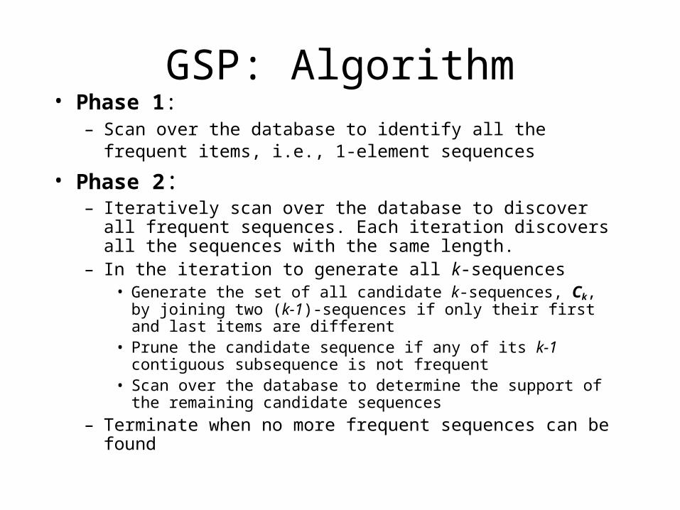
GSP: Algorithm• Phase 1:

– Scan over the database to identify all the frequent items, i.e., 1-element sequences

• Phase 2: – Iteratively scan over the database to discover all frequent

sequences. Each iteration discovers all the sequences with the same length.

– In the iteration to generate all k-sequences • Generate the set of all candidate k-sequences, Ck, by joining

two (k-1)-sequences if only their first and last items are different• Prune the candidate sequence if any of its k-1 contiguous

subsequence is not frequent • Scan over the database to determine the support of the

remaining candidate sequences

– Terminate when no more frequent sequences can be found

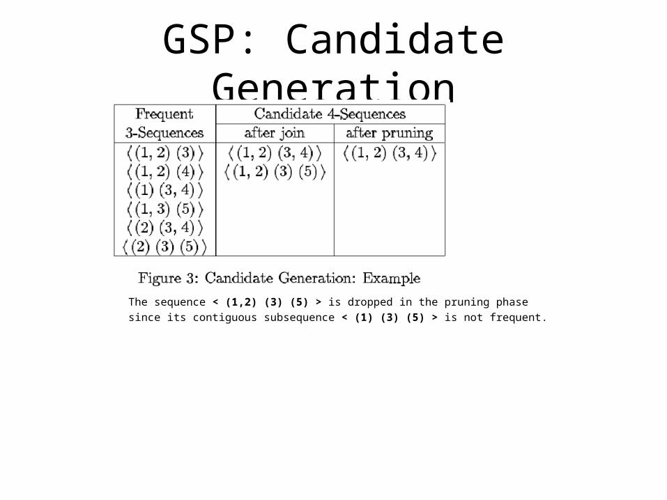
GSP: Candidate Generation

The sequence < (1,2) (3) (5) > is dropped in the pruning phase

since its contiguous subsequence < (1) (3) (5) > is not frequent.

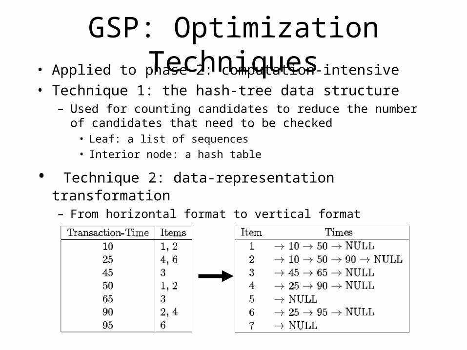
GSP: Optimization Techniques• Applied to phase 2: computation-intensive• Technique 1: the hash-tree data structure

– Used for counting candidates to reduce the number of candidates that need to be checked

• Leaf: a list of sequences

• Interior node: a hash table

• Technique 2: data-representation transformation– From horizontal format to vertical format

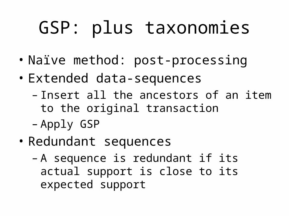
GSP: plus taxonomies

• Naïve method: post-processing

• Extended data-sequences– Insert all the ancestors of an item to the

original transaction– Apply GSP

• Redundant sequences– A sequence is redundant if its actual support

is close to its expected support

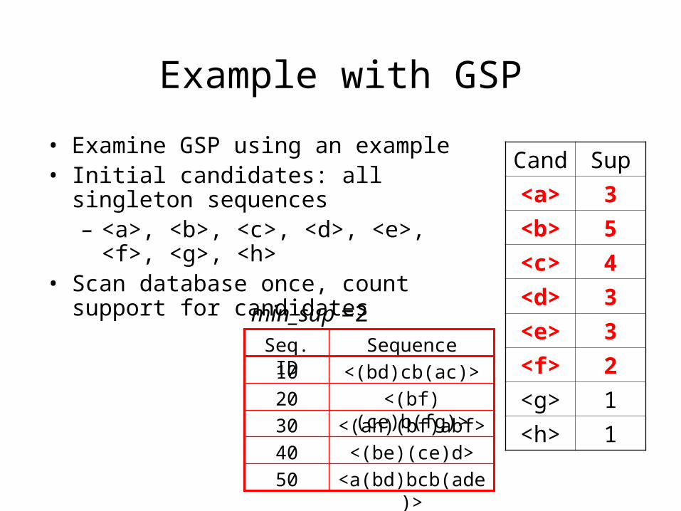
Example with GSP

• Examine GSP using an example • Initial candidates: all singleton

sequences– <a>, , <c>, <d>, <e>, <f>, <g>,

<h>• Scan database once, count support for

candidates

<a(bd)bcb(ade)>50

<(be)(ce)d>40

<(ah)(bf)abf>30

<(bf)(ce)b(fg)>20

<(bd)cb(ac)>10

SequenceSeq. ID

min_sup =2

Cand Sup

<a> 3

 5

<c> 4

<d> 3

<e> 3

<f> 2

<g> 1

<h> 1

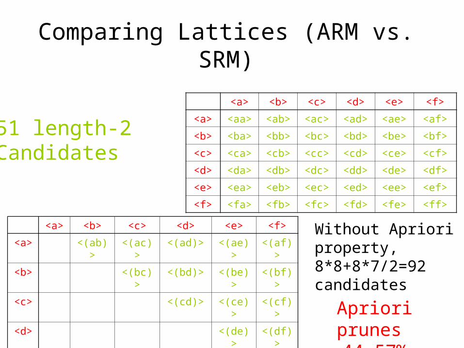
Comparing Lattices (ARM vs. SRM)

<a> <c> <d> <e> <f>

<a> <aa> <ab> <ac> <ad> <ae> <af>

 <ba> <bb> <bc> <bd> <be> <bf>

<c> <ca> <cb> <cc> <cd> <ce> <cf>

<d> <da> <db> <dc> <dd> <de> <df>

<e> <ea> <eb> <ec> <ed> <ee> <ef>

<f> <fa> <fb> <fc> <fd> <fe> <ff>

<a> <c> <d> <e> <f>

<a> <(ab)> <(ac)> <(ad)> <(ae)> <(af)>

 <(bc)> <(bd)> <(be)> <(bf)>

<c> <(cd)> <(ce)> <(cf)>

<d> <(de)> <(df)>

<e> <(ef)>

<f>

51 length-2Candidates

Without Apriori property,8*8+8*7/2=92 candidates

Apriori prunes 44.57% candidates

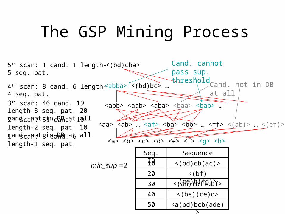
The GSP Mining Process

<a> <c> <d> <e> <f> <g> <h>

<aa> <ab> … <af> <ba> <bb> … <ff> <(ab)> … <(ef)>

<abb> <aab> <aba> <baa> <bab> …

<abba> <(bd)bc> …

<(bd)cba>

1st scan: 8 cand. 6 length-1 seq. pat.

2nd scan: 51 cand. 19 length-2 seq. pat. 10 cand. not in DB at all

3rd scan: 46 cand. 19 length-3 seq. pat. 20 cand. not in DB at all

4th scan: 8 cand. 6 length-4 seq. pat.

5th scan: 1 cand. 1 length-5 seq. pat.

Cand. cannot pass sup. threshold

Cand. not in DB at all

<a(bd)bcb(ade)>50

<(be)(ce)d>40

<(ah)(bf)abf>30

<(bf)(ce)b(fg)>20

<(bd)cb(ac)>10

SequenceSeq. ID

min_sup =2

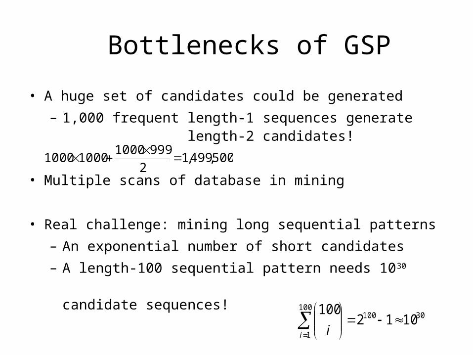
Bottlenecks of GSP

• A huge set of candidates could be generated

– 1,000 frequent length-1 sequences generate length-2 candidates!

• Multiple scans of database in mining

• Real challenge: mining long sequential patterns

– An exponential number of short candidates

– A length-100 sequential pattern needs 1030 candidate sequences!

500,499,12

999100010001000

30100100

1

1012100

i i

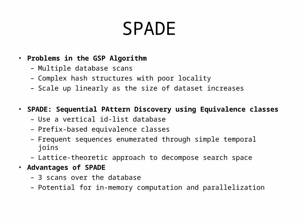
SPADE

• Problems in the GSP Algorithm– Multiple database scans– Complex hash structures with poor locality– Scale up linearly as the size of dataset increases

• SPADE: Sequential PAttern Discovery using Equivalence classes – Use a vertical id-list database– Prefix-based equivalence classes– Frequent sequences enumerated through simple temporal joins– Lattice-theoretic approach to decompose search space

• Advantages of SPADE– 3 scans over the database– Potential for in-memory computation and parallelization

Recent studies: Mining Constrained Sequential patterns

• Naïve method: constraints as a post-processing filter– Inefficient: still has to find all patterns

• How to push various constraints into the mining systematically?

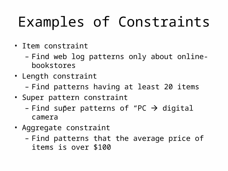
Examples of Constraints

• Item constraint– Find web log patterns only about online-bookstores

• Length constraint– Find patterns having at least 20 items

• Super pattern constraint– Find super patterns of “PC digital camera”

• Aggregate constraint– Find patterns that the average price of items is over

$100

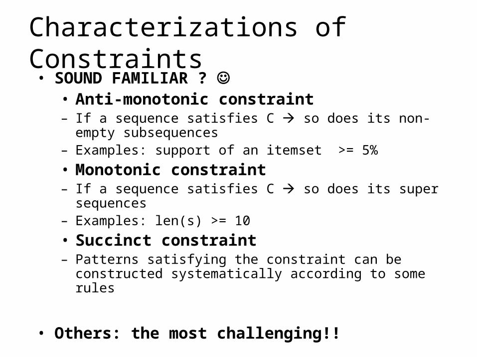
Characterizations of Constraints• SOUND FAMILIAR ?

• Anti-monotonic constraint– If a sequence satisfies C so does its non-empty subsequences– Examples: support of an itemset >= 5%

• Monotonic constraint– If a sequence satisfies C so does its super sequences– Examples: len(s) >= 10

• Succinct constraint– Patterns satisfying the constraint can be constructed systematically

according to some rules

• Others: the most challenging!!

Covered in Class Notes (not available in slide form

Scalable extensions to FPM algorithms– Partition I/O– Distributed (Parallel) Partition I/O– Sampling-based ARM

Association Rules Outline Goal: Provide an overview of basic Association Rule mining techniques...

Documents

Transcript of Association Rules Outline Goal: Provide an overview of basic Association Rule mining techniques...