Rotor concepts and load estimation

Assoc. Prof. Martin O.L.HansenDTU Wind Energy and CeSOS, NTNU

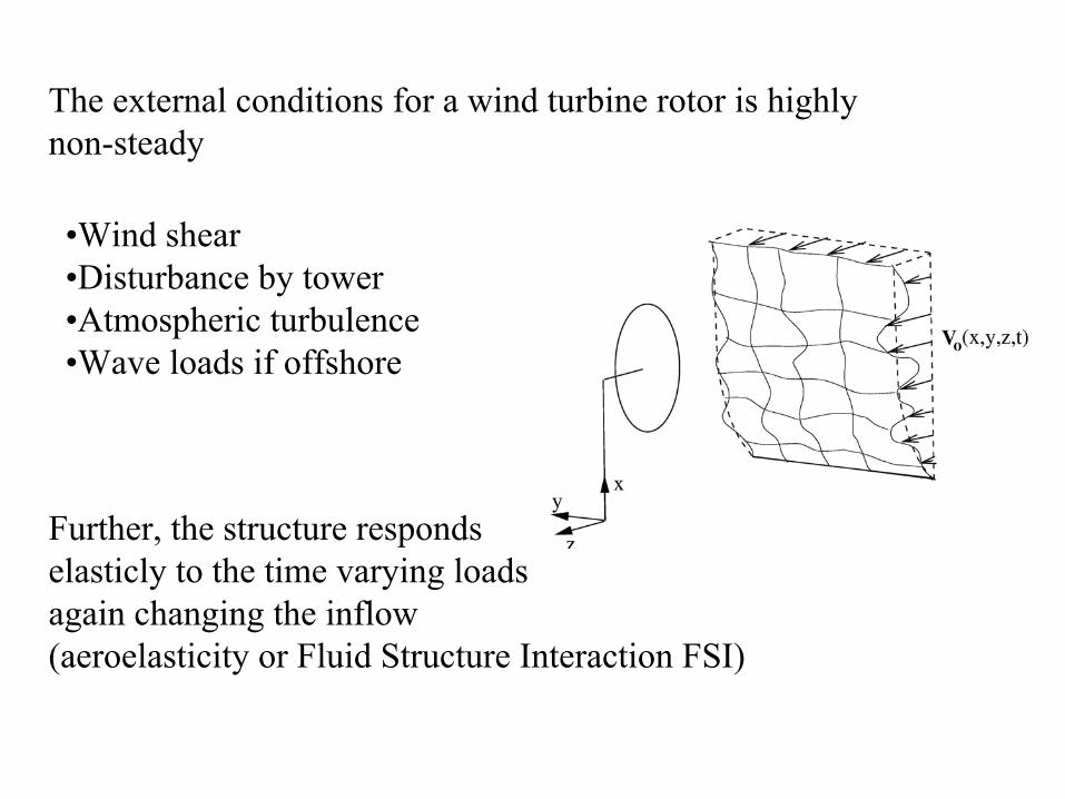
Inflow•Wind shear•Disturbance

by tower

•Atmospheric

turbulence•Wave

loads

if

offshore

The external

conditions

for a wind

turbine rotor is highlynon-steady

Further, the structure

respondselasticly

to the time varying

loads

again

changing

the inflow(aeroelasticity

or

Fluid Structure

Interaction

FSI)

The aerodynamic

model is called

many

times during

a time simulationof the structural

dynamics

Typical

simulation time T=600 s and timestep Δt=0.01s, i.ein the order

of 60000 iterations

per load case

Number

of simulations is in the order

of 2000 load cases !!!!(120 mill. calls)

A FAST MODEL IS REQUIRED

Therefore

engineering

models such

as the Blade Element Momentummodel (BEM) still widely

used

( ) ( )m A x u x

2 210 12 ( )kinEP m V u

t

The most basic slide understanding a wind turbine:A force is needed (thrust T) to slow down the wind speed in order to extract kinetic energy per time, P, from the flow approaching the rotor

2p Vr r

The thrust force can be achieved as a pressure drop created by flow past a wingT=p·A

The local

flow on

a HAWT wind

turbine rotorneglecting

”induced

wind”

Aerodynamic

loads

on

a 2-D wing section

212

( ,Re)lLCV c

212

( ,Re)dDCV c

Real flow past

blade including

induced

wind

We learned that the power comes from removing kinetic energy from the air through creating a force pointing upstream (thrust)

( ) ( )m A x u x

Should we then not increase the thrust until the velocity in the wake u1 =0 ?

2 210 12 ( )kinEP m V u

t

The answer is no

If ones

increases

T too

much

then

the flow will

go around

the rotorandif

T=0, then 1 0u V0m

In both

cases the power is 0 and an optimum value

must exist

2 210 12 ( )P m V u

It can be shown that u=½(Vo

-u1

)

2 210 12

2 2 2 2 21 10 1 0 0 02 2

20

32 10 03 2

( )

( ) ( ( 2 ) ) 2 ( )

/ 2 (2 3 ) 01627opt opt

P m V u

P Au V u Au V V u Au V u

dP du A uV u

u V P A V

312

po

PCV A

312

,max 312

161627 60%27

o

po

V AC

V A

Definition power coefficient

Theoretical

maximum

Betz limit

How big must T be to obtain this ?

)()( 10101110 uVAVAAuAVAm cvcvside

200

201

211 )( VAVmVAAuAT cvsidecv

)()( 101011 uVAuuVuAT

Conservation

of momentum: ( )CV CS

d Volt

V V V dA F

0 1

22 1 10 0 0 03 3 2

( )

8( )9opt

T Au V u

T A V V V A V

2102

TTCAV

21

02

, 2102

8899T opt

A VC

AV

Definition thrust

coefficient Optimum value

(Betz

limit)

Conservation

of momentum

Measured

CT

(a)U=(1-a)VoMomentum theory

not valid for high

CT

]/[cossin]/[sincos

mNDLpmNDLp

T

N

Lift and drag projected

relative to rotorplane

Lift and drag responsible

for thrust

and torque

!!!

NT p dr R T

R

M rp dr

P M

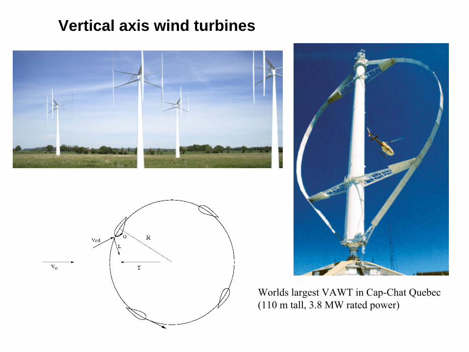
Worlds largest VAWT in Cap-Chat Quebec(110 m tall, 3.8 MW rated power)

Vertical axis wind turbines

rel rot oV V W V

cos sinsin cos

n

t

p L Dp L D

Velocity

triangle

gives size

of relativevelocity

and angle to rotor f

212

212

( )

( )

p

rel l

rel d

L V cC

D V cC

Lift and drag projected

normal to rotor (L

is normal to Vrel

)

If the tangential load is known the power can be computed as

1

1 13 3 31 1

2 2

( ) ( )

( )( )2 2

B

tot t

B B

t t

po o o

P t M t p hR

p hR pP tC tV h R V h R V

For both the HAWT and the VAWT wind turbine the angle of attack can be estimated if the induced wind, W, is known

If the angle of attack is known the aerodynamic lift and drag can be estimated from 2-D airfoil data

From the aerodynamic loads the global power and thrust can be calculated

The induced wind can be estimated 1) from the basic conservation of momentum equations (engineering method)

or alternatively 2) the

flow and thus the loads can be computed using CFD

HAWT

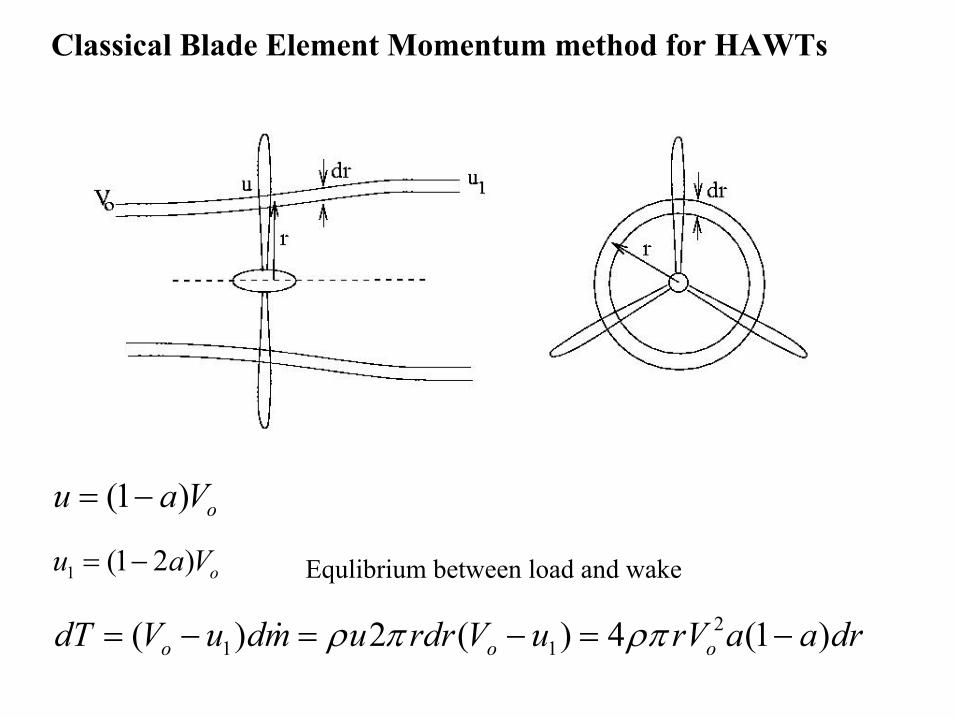
21 1( ) 2 ( ) 4 (1 )o o odT V u dm u rdr V u rV a a dr

(1 ) ou a V

1 (1 2 ) ou a V

Classical

Blade Element Momentum method

for HAWTs

Equlibrium

between

load and wake

( cos sin )NdT Bp dr B L D dr

( cos sin )NdT Bp dr B L D dr

24 (1 )odT rV a a dr

Two

different

equations

for the local

thrust

force

cos sinn l dC C C

2Bc

r

21

4 sin 1n

aF

C

Similarly

can

be

derived

for tangential

induction

a’=wtan

/ωr

2Bc

r

( sin cos )TdM Brp dr Br L D dr

34 (1 )odM r V a a dr

sin cost l dC C C

14 sin cos 1

t

a FC

For high

CT the momentum theory

not valid (Glauert

correction)

13

1 14 3

4 (1 )4 (1 (5 3 ) )T

a a F aC

a a a F a

Empirical correlation

Comparison between computed and measured electrical power for the 2MW Tjaereborg

machine

The classical BEM gives good results for the steady loads

Can

be

used

as a preprocessor

to a WT controller

to estimate

the maximumpower coefficient

and the necessary

pitch

and tip speed ratio

Cp,max

(θp

,)

and the gains

in a PI controller

The classical BEM code only valid for constant inflowand zero yaw.

Can be used to calculate power curves –

but not for unsteadycalculation of the loads during operation

This can be cured adding some engineering models

Unsteady

BEM (Vo

(t), Vrel

(t), α(t)) fi L(t) and D(t)

(t)

(t)

cos4 )n

g

BLWrF f

o nV W

sin4 )t

g

BLWrF f

o nV W

Quasi steady induced velocities calculated as:

The equations

for the induced

velocity

consistent

withmomentum theory

for zero

yaw

The equations are also valid for 90 degrees yaw (basic helicopter theory)

And it is therefore assumed they are valid for any yaw angle !!!

Unsteady effects

intint 1 1

qsqs

dWdWW W kdt dt

2 intdWW Wdt

Dynamic inflow/wakeDynamic inflow/wake

Dynamic stall

These

and similar

equations

are

the basis for the assesment

of the aerodynamic

loads

in most servo-,hydro,-aeroelastic

codes

such

as e.g.

HAWC2FLEX5BLADEDFAST

VAWTsAlso

for vertical

axis

wind

turbines the momentum based

method

are

popular

Single discDouble disc

Single disc theory

Relationship

between

the local

thrust

in a streamtube

and thedecreased

local

velocity

u that

includes

the induced

velocity

Step 1: Calculate

aerodynamic

loadsfrom assumed

value

of induced

wind

,

,

2 2 2, ,

rel x o x

rel y

rel rel x rel y

V V y WV x

V V V

, ,

, ,

sin cos

cos sin

atan( / )

t rel y rel x

r rel y rel x

r t

p

V V V

V V V

V V

212

212

( )

( )rel l

rel d

L V cC

D V cC

, ,

,,

rel y rel xx

rel rel

rel yrel xy

rel rel

V Vp L D

V VVV

p L DV V

Step 2: Estimate

mean

axial

load

2

2x x

x

N

B p B ppN

Step 3: Calculate

thrust

coefficient

212

xT

o

pCV h

Step 4: Update

induced

velocity

(induction

factor a)

13

1 14 3

(1 )

4 (1 )4 (1 (5 3 ) )

x

o

o

T

WaV

u a V

a a aC

a a a a

Solve

for a new a

and thus

Wx

then

goto

step 1

Double disc to simulate

also

the downstream

part of the rotor

Free wind speed approaching rotor(1 ) wind speed at upstream disc(1 2 ) Inflow to downstream disc(1 ) wind speed at downstream disc

u u

e u

d d e

UU a UU a UU a U

au and ad found

similarly

as in single disc from CT

(a) relation

CFD

0

ij

jiij

j i

D pDt

uux x

V

V g

Numerical solution of the Navier-Stokes equations

Incompressible N-S equations

From ICEM CFD Engineering

-Preprocessor (where a lot of time is spent)•Geometry (CAD or similar)•Grid generator•Specifying boundary conditions (inflow, outflow, wall, symmetry etc.)

-Solver•Steady/unsteady•Discretization (Upwind schemes)•Turbulence model•Transition model

-Postprocessor•extract specific data•visualization

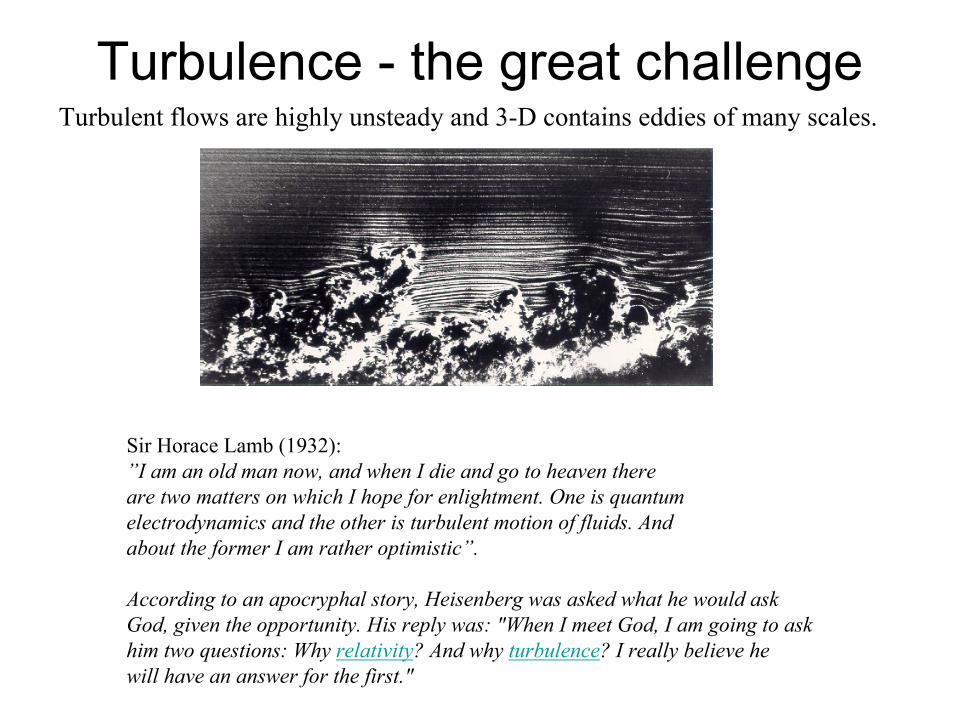
Turbulence

-

the great

challengeTurbulent flows are

highly

unsteady

and 3-D contains

eddies

of many

scales.

Sir Horace Lamb

(1932):”I am an old

man now, and when

I die and go to heaven

thereare

two

matters

on

which

I hope

for enlightment. One is quantumelectrodynamics

and the other

is turbulent motion of fluids. And about

the former I am rather

optimistic”.

According to an apocryphal story, Heisenberg was asked what he would ask God, given the opportunity. His reply was: "When I meet God, I am going to askhim two questions: Why relativity? And why turbulence? I really believe hewill have an answer for the first."

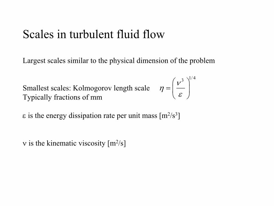
Scales

in turbulent fluid flow

Largest

scales

similar

to the physical

dimension of the problem

Smallest scales: Kolmogorov

length

scaleTypically

fractions

of mm

is the energy

dissipation

rate per unit mass

[m2/s3]

is the kinematic

viscosity

[m2/s]

1/ 43

Number

of gridpoints

required

for a Direct

Numerical

Simulation (DNS)

Re9/4

Example

:

Re=105 N=1.8·1011

Re=106

N=3.2·1013

Modeling the turbulence therefore necessary

Reynolds averaging

of the equations

RANS

0

1 ( )

0

T

f f f g g g

f f t dtT

f ff f g f gs s

gf gf

u u u v v v w w w p p p

Following

is set into

the NS equations

Afterwards

the NS equations

are

timeaveraged

usingthe formulaes

from previous

slide as:

ij

jiij

j i

D pDt

uux x

V g

The result

becomes

' '( )ij i jD p u uDt

V g

This

is the standard NS equations

with

an addedterm denoted

the Reynolds stresses (stress tensor)

' 'turbij i ju u

Transport equations

can

be

derived

for the Reynoldsstresses, but this

introduces

terms of third

order

products

of the fluctuating

velocities.

This

is known

as the closure

problem.

' ' 23

jturb iij i j t ij

j i

uuu u kx x

Boussinesq

approximation

therefore

models theReynold’s

stresses through

an eddy

viscosity

t

23 ijkIf the term is added

to the pressure

the equations

becomes

similar

to the normal NS equations

*

*

( )

23

ij

jiij t

j i

D pDt

uux x

p p k

V g

Turbulence

is modeled

as an extra

diffusionand the role

of the turbulence

model is to calculate

the size

of this

diffusion

Different

catogories

of turbulence

models:

Algebraic

One-equation

models

Two

equations

models

RNG (ReNormalization

Group)

Reynolds stress models

LES (Large Eddy

Simulation)

DES (Deatached

Eddy

Simulation)

DNS (Direct

Numerical

Simulation)

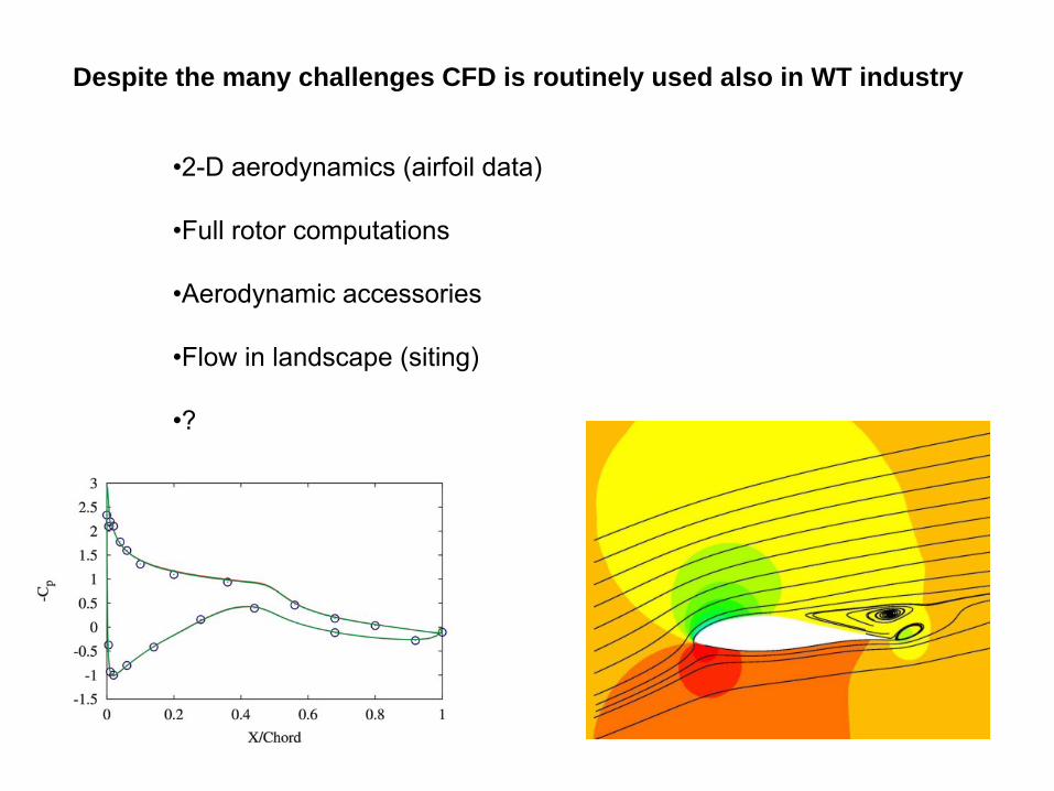
Despite the many challenges CFD is routinely used also in WT industry

•2-D aerodynamics (airfoil data)

•Full rotor computations

•Aerodynamic accessories

•Flow in landscape (siting)

•?

NREL Wind tunnel measurement

NASA Ames Tunnel (24.4x36.6 m)NREL Phase-VI Wind Turbine

Breaktrough of CFD for wind turbine rotors

Blind test comparisonUpwind Configuration, Zero Yaw

0

500

1000

1500

2000

2500

3000

3500

4000

5 10 15 20 25

Wind Speed (m/s)

Low

-Spe

ed S

haft

Torq

ue (N

m)

Risø comp.

measurements

∎

Pressure distributions at 7 m/s

Pressure distributions at 10 m/s

CFD for wind turbine rotors

AdvantagesFull control over input parametersCheap compared to measurementsParametric variations can easily be madeProvides detailed information of the very complex flow everywhere in the field Input to faster empirical engineering type modelsGain knowledge of complex flow physics

DisadvantagesLarge computer resourcesPrediction of separation,

turbulence and transition modellingSlow compared to BEM, not suited for realistic aeroelastic

simulationsGrid generation… ?