Asset Pricing Theory Option A right to buy (or sell) an underlying asset. Strike price: K Maturity...

Asset Pricing Theory

Option

A right to buy (or sell) an underlying asset.

Strike price: K Maturity date: T. Price of the underlying asset: S(t)

Asset Pricing Theory

Price of the call option at maturity:

Price of the put option at maturity:

)0,)(( KTSMax

)0),(( TSKMax

Binomial Asset Pricing Model

S(t) : price of stock at time t V(t) : price of the option at time t

S0

S1(H)=uS0

S1(T)=dS0


V0

V1(H)=Max(uS0-K,0)

V1(T)=Max(dS0-K,0)


Replicate Suppose there are two assets.

Asset 1: Option with price V(t) at time t.

Asset 2: Portfolio of Stock and Saving

account (or Bond)


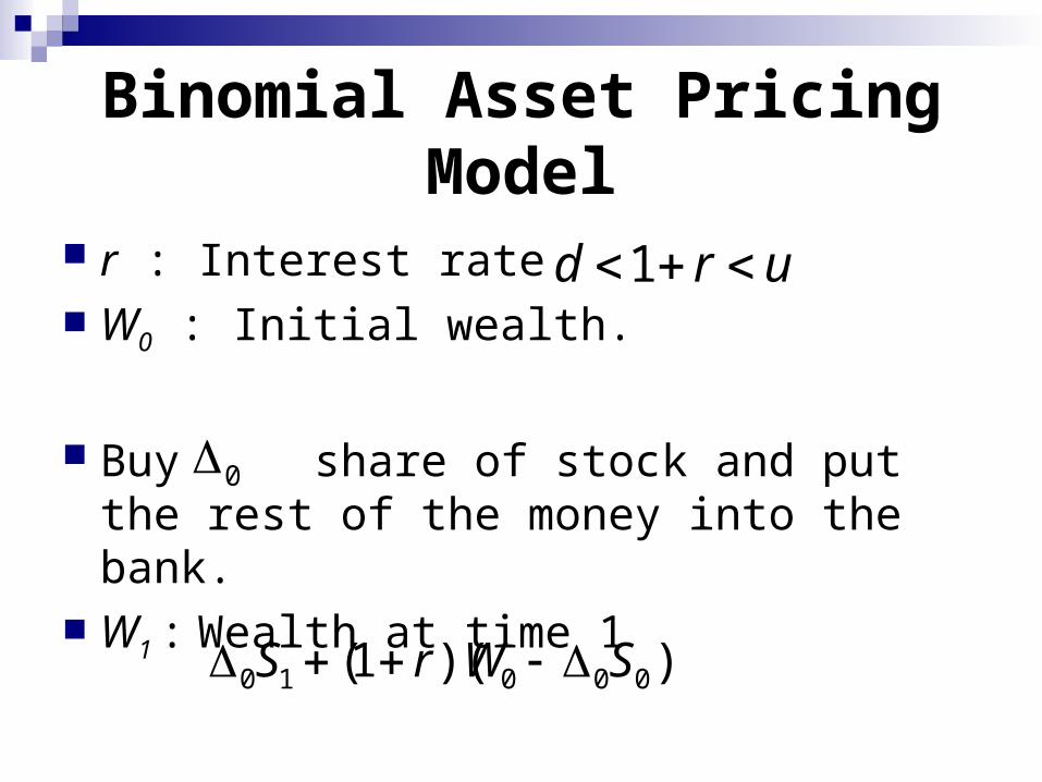
r : Interest rate W0 : Initial wealth.

Buy share of stock and put the rest of the money into the bank.

W1 : Wealth at time 1

1d r u

0

))(1( 00010 SWrS


)0,)(max()())(1(

)0,)(max()())(1()(

1100010

1100010

KTSTVSWrS

KHSHVSWrHS

1 10

1 1

( ) ( )

( ) ( )

V H V T

S H S T

)(

)1()(

1

1

1110 TV

du

rdHV

du

ur

rW


No Arbitrage Asset 1 =Asset 2 Option price V0 = W0

0 1 1

1 1

1 1 (1 )[ ( ) ( )]

11

[ ( ) ( )]1

r d u rV V H V T

r u d u d

pV H qV Tr


one step binomial model APT

where

)(~

)](~)(~[ 111

1111

0 VETVqHVpV rr

duru

dudr qp

)1()1( ~,~


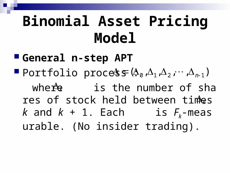
General n-step APT Portfolio process :

where is the number of shares of stock held between times k and k + 1. Each is Fk-measurable. (No insider trading).

),,,,( 1210 n

k

k


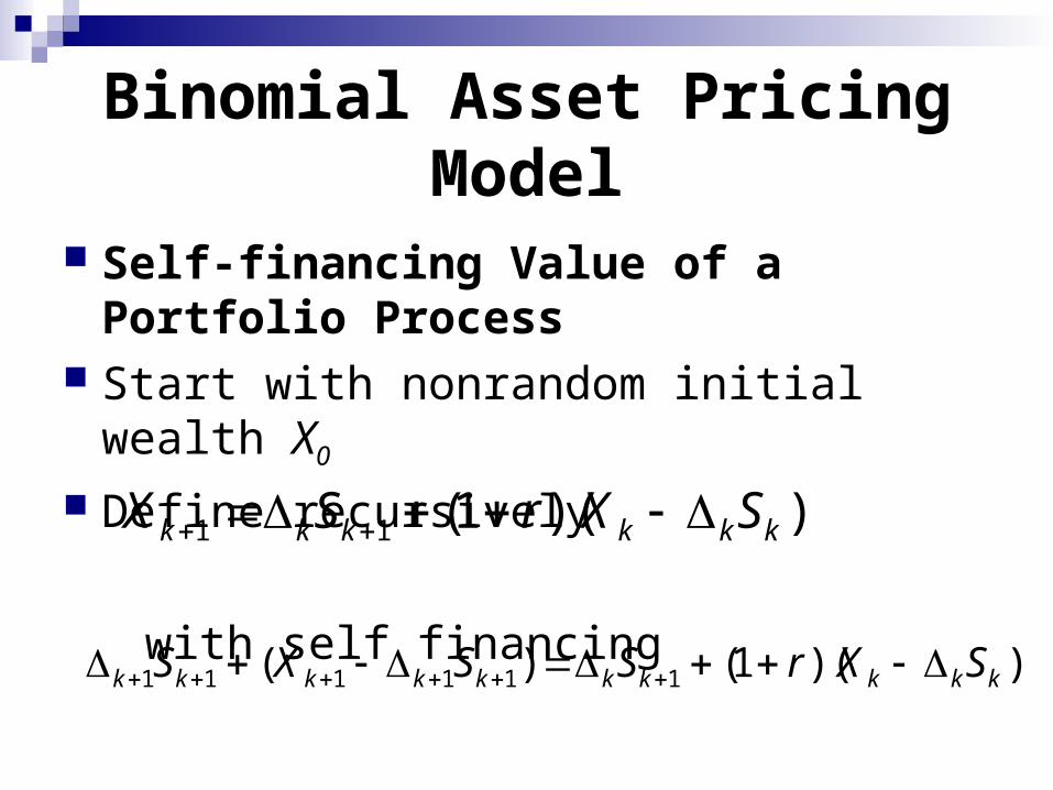
Self-financing Value of a Portfolio Process

Start with nonrandom initial wealth X0

Define recursively

with self financing

))(1(11 kkkkkk SXrSX

))(1()( 111111 kkkkkkkkkk SXrSSXS


APT value of the simple European asset at time k is

)|)1((~

)1( kmmk

k FVrErV

Random Walks

Symmetric random walk

sequence of Bernoulli trial with p = 0.5.

1}{ iiY

00 M

k

iik YM

1

Random Walks

E(Mk)=0

var(Mk)=k

If k < m, then Mk and Mm – Mk are independent

Brownian Motion

The Law of Large Number Central Limit Theorem Brownian Motion as a Limit of Random

Walk The Limit of a Binomial Model

Brownian Motion

Let Consider a Random walk with time lag

and space lag , , which is defined by

, then

ttYYYM t

t

21

tt t

tZ

)( 21ttYYYtMtZ t

tt

t

Brownian Motion

ondistributiin )(

)(1lim

)(limlim

210

2100

tB

YYYt

YYYtZ

tt

tt

ttt

t

tt

t

Brownian Motion

A random variable B(t) is called a Brownian Motion (Wiener Process) if it satisfies the following properties:

B(0) = 0, B(t) is a continuous function of t; B has independent, normally distributed increme

nts: If 0 = t0 < t1 < t2 < ...< tn and

)()(,),()(),( 112211 nnn tBtBYtBtBYtBY

Brownian Motion

then

(1). are independent

(2). for all j.

(3). for all j.

nYYY ,,, 21 0][ jYE

1]var[ jjj ttY

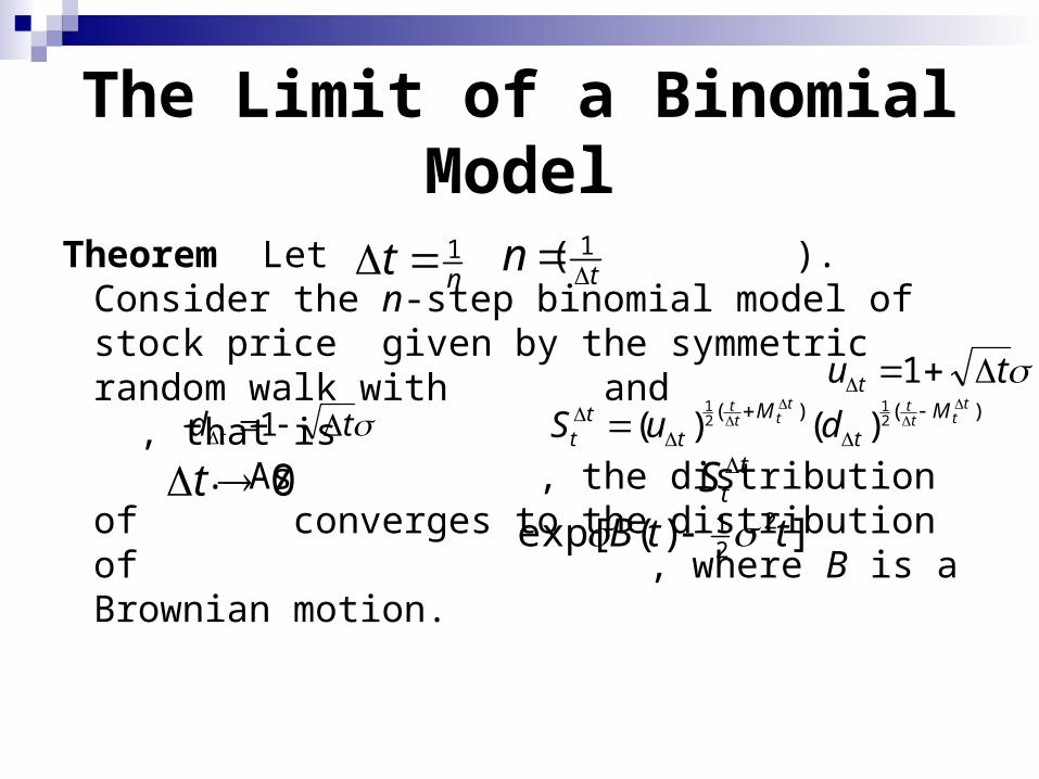
The Limit of a Binomial Model

Consider the n-step Binomial model with

Let , and

tn 1

tu t 1 td t 1 10 tS


Theorem Let ( ). Consider the n-step binomial model of stock price given by the symmetric random walk with and , that is . As , the distribution of converges to the distribution of , where B is a Brownian motion.

nt 1 tn 1

tu t 1

td t 1 )()( 21

21

)()(t

tttt

ttt M

tM

tt

t duS

0t ttS

])(exp[ 221 ttB

The Itô Integral

First Variation Quadratic Variation Quadratic Covariation pth Finite Variation Riemann-Stieltjes integral

The Itô Integral

The Itô Integral

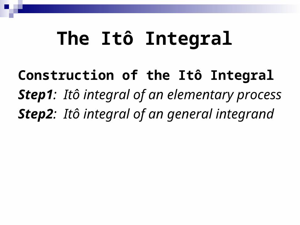
Construction of the Itô Integral

Step1: Itô integral of an elementary process

Step2: Itô integral of an general integrand

The Itô Integral

Think of B(t) as the price per unit share of an asset at time t.

Think of t0; t1; … ; tn as the trading dates for the asset.

Think of δ(tk) as the number of shares of the asset acquired at trading date tk and held until trading date tk+1.

The Itô Integral

The total gain is

We define

))()()(())()()(()(1

1 11 kk

k

i iii tBtBttBtBttI

t

udButI0

)()()(

The Itô’s formula

Taylor’s formula3

!312

!21 ))(())(())(()()( axbfaxafaxafafxf

3

222!2

1

||

)])()(,,(2

))()(,,(2))()(,,(2

))(,,())(,,())(,,([

))(,,())(,,())(,,(

),,(),,(

O

cybxcbaf

cyatcbafbxatcbaf

cycbafbxcbafatcbaf

cycbafbxcbafatcbaf

cbafyxtf

xy

tytx

yyxxtt

yxt


Differential

Let f be differentiable. Then the differential of f is

Define , then

df is an infinitesimal change of dependent variable as there is a small change dx for the independent variable.

dxxfdf )()()( xfdxxff dff


Chain rules Let f and g be differentiable functions. Set . Then the differential

dz is an infinitesimal change of dependent variable as there is a small change dx for the independent variable.

))(( xgfz

dxxgxgfdgxgfdz )())(())((


The path of a Brownian motion is not differentiable everywhere.

Set .

Since

and .

We denote . (ie )

)()()( tBdttBtdB 0))()(( 2 dttBdttBE

22 )(2))()(( dttBdttBVar dttdBtdB )()( dttdB )(


Itô’s Formula 1

Itô’s Formula 2

dttBftdBtBftBdf ))(()())(())(( !21

dttBtfdBtBtfdttBtftBtdf xxxt ))(,())(,())(,())(,( !21


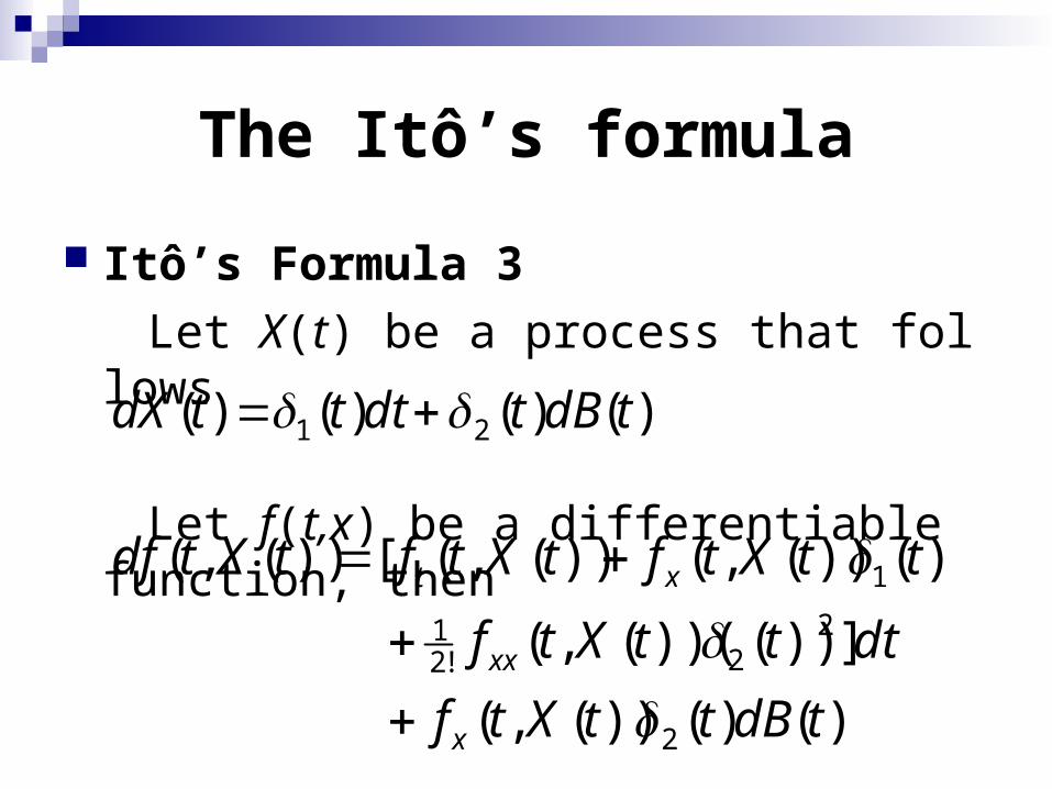
Itô’s Formula 3

Let X(t) be a process that follows

Let f(t,x) be a differentiable function, then)()()()( 21 tdBtdtttdX

)()())(,(

]))())((,(

)())(,())(,([))(,(

2

22!2

1

1

tdBttXtf

dtttXtf

ttXtftXtftXtdf

x

xx

xt


Itô’s Formula 4

)()()()( 1211 tdBtdtttdX

)()()()( 2221 tdBtdtttdY

)]()())(),(,(

)()())(),(,(2

)()())(),(,([

)())(),(,(

)())(),(,())(),(,())(),(,(

!21

tdYtdYtYtXtf

tdYtdXtYtXtf

tdXtdXtYtXtf

tdYtYtXtf

tdXtYtXtfdttYtXtftYtXtdf

yy

xy

xx

y

xt


dtttdYTdY

dttttdYtdX

dtttdXtdX

)()()(

)()()()(

)()()(

222

2212

212

Applications of The Itô’s Formula

Stock process :

Return:

)()()( tSdttStS )()()( tSdttStdS

)()(

)()()(

tStdS

tStSdttS

dttE tStdS )()()( dttVar tS

tdS )(2)()(

)()()()()()( tdBtStdttSttdS


Geometric Brownian Motion

An investor begins with nonrandom initial wealth X0 and make the self finance wealth X(t) at each time t by holding shares of stock that follows the Geometric Brownian Motion and financing his investment by a bond with interest rate r.

)()()()( tdBtSdttStdS

)(t


dttSttXrtdSttdX ))()()(()()()(

dttSttXrtdBtSdttSt ))()()(())()()()((

))()()()]())(()([ tdBtStdttSrttrX


Consider an European option that use stock S(t) as underlying asset with the terminal payoff . Let be the price of the option at time t. Then

))(( TSg ))(,( tStv

)()()())(,( 21 tdStdSvtdSvdtvtStdv SSSt

dttSvtdBtSdttSvdtv SSSt )()]()()([ 2221

)()(])()([ 2221 tdBtSvdtvtSvtSv SSSSt


A hedging portfolio starts with some initial wealth X0 and invests so that the wealth X(t) at each time tracks . To ensure

for all t, the coefficients before the differential of X(t) and must be equal.

))(,( tStv

))(,()( tStvtX ))(,( tStdv


and

Therefore

))(,()( tStvt S

)())(()()()( 2221 tSrttrXvtSvtSv SSSt

rvvtSvtrSv SSSt )()( 2221


Black-Scholes PDE

)(),(

2221

xgxTv

rvvxrxvv xxxt

Kolmogorov PDE

Let be the solution Stochastic DE

Set . Then is the

solution of the Kolmogorov backward PDE

xX

dWXbdtXadX tttt

0

)()(

xtt XX

)]([),( xtXfExtu ),( xtu

).(),0(

),()(),()(),( 2!2

1

xfxu

xtuxaxtuxbxtu xxxt

Feynman-Kac Theorem

Suppose that Xs satisfies the SDE

for

Then if and only if satisfies the backward Kolmogorov PDE

xX

dWXsbdsXsadX

t

ssss ),(),(Tst

]|)([),,(),(

xXXfeExTtu tT

duXurT

tu

),,( xTtu

)(),,(

0),(),(),( 221

xfxTTu

uxtruxtbuxtau xxxt

Asset Pricing Theory Option A right to buy (or sell) an underlying asset. Strike price: K Maturity...

Documents

Transcript of Asset Pricing Theory Option A right to buy (or sell) an underlying asset. Strike price: K Maturity...