Asset-Pricing Anomalies at the Firm Level

Scott Cederburg∗ Phil Davies† Michael O’Doherty‡

April 18, 2011§

Abstract

Portfolio-level tests linking CAPM alphas to a large number of firm characteristics suggest

that the CAPM fails across multiple dimensions. There are, however, concerns that underlying

firm-level associations may be distorted at the portfolio level. In this paper we use a hierarchical

Bayes approach to model conditional firm-level alphas as a function of firm characteristics. Our

empirical results indicate that much of the anomaly-based evidence against the conditional

CAPM is overstated. Anomalies are primarily confined to small stocks, few characteristics are

robustly associated with CAPM alphas out of sample, and the majority of firm characteristics

do not contain unique information about abnormal returns.

JEL Classification: C11, G10, G12, G14

∗Tippie College of Business, University of Iowa, S217 Pappajohn Business Building, Iowa City, IA 52242. Email:scott-cederburg@uiowa.edu. Tel: (319) 541-5726.†Rutgers Business School, 1 Washington Park, Newark, NJ 07102. Email: pdavies@andromeda.rutgers.edu.‡Tippie College of Business, University of Iowa, S319 Pappajohn Business Building, Iowa City, IA 52242. Email:

michael-odoherty@uiowa.edu. Tel: (319) 335-0974.§We thank Doron Avramov, Ashish Tiwari, Paul Weller, Tong Yao, and seminar participants at Iowa State

University, the University of Iowa, the University of Nebraska–Lincoln, the 2010 CRSP Forum, the 2011 EasternFinance Association, and the 2011 Midwest Finance Association for helpful comments and suggestions.

1 Introduction

An anomaly is a pattern in average stock returns that is inconsistent with the predictions

of the Capital Asset Pricing Model (CAPM) of Sharpe (1964) and Lintner (1965). Anomalies

are commonly identified using a portfolio-based approach. The researcher sorts stocks on a firm

characteristic and constructs a zero-cost hedge portfolio by taking long and short positions in

the extreme groups. If the hedge portfolio earns abnormal returns relative to the CAPM, the

sorting characteristic is classified as an anomaly. Over the past three decades, a large number

of anomalies have been uncovered, suggesting the CAPM is unable to explain much of the cross-

sectional variation in average stock returns.1

There are, however, growing concerns in the literature about the use of portfolios to identify

anomalies and, more generally, to test asset-pricing models. These arguments are centered around

the idea that grouping firms into portfolios and aggregating returns wastes and potentially distorts

valuable information about cross-sectional patterns in abnormal returns. For example, Roll (1977),

Kandel and Stambaugh (1995), and Fama and French (2008) discuss how patterns in firm-level

pricing errors can be distorted at the portfolio level. Lo and MacKinlay (1990) highlight the data-

snooping biases inherent in portfolio-based asset-pricing tests, while Litzenberger and Ramaswamy

(1979) and Ang, Liu, and Schwarz (2010) consider the loss in efficiency from using portfolios rather

than individual firms in asset-pricing tests. More recently, Ahn, Conrad, and Dittmar (2009) and

Lewellen, Nagel, and Shanken (2010) show that inferences in asset-pricing tests are sensitive to the

choice of test portfolios.2

One way to avoid the concerns with portfolio-level inferences is to use firm-level data. However,

examining anomalies at the firm level is a challenging problem. The researcher has to relate firm

characteristics to abnormal returns which are not directly observable. Therefore, the researcher

must also model and estimate the evolution of market risk for each individual firm.

Two recent firm-level studies adopt contrasting approaches to control for market risk. Fama

1Previous papers show a positive relation between average returns and book-to-market equity (Rosenberg, Reid,and Lanstein (1985), Chan, Hamao, and Lakonishok (1991), and Fama and French (1992)), stock return momentum(Jegadeesh (1990) and Jegadeesh and Titman (1993, 2001)), and profitability (Haugen and Baker (1996) and Cohen,Gompers, and Vuolteenaho (2002)). There is a negative relation between average returns and size (Banz (1981) andFama and French (1992)), stock return reversal (DeBondt and Thaler (1985) and Chopra, Lakonishok, and Ritter(1992)), asset growth (Fairfield, Whisenant, and Yohn (2003), Titman, Wei, and Xie (2004), and Cooper, Gulen, andSchill (2008)), net stock issues (Loughran and Ritter (1995), Ikenberry, Lakonishok, and Vermaelen (1995), Danieland Titman (2006a), and Pontiff and Woodgate (2008)), accruals (Sloan (1996), Collins and Hribar (2000), and Xie(2001)), and financial distress (Dichev (1998) and Campbell, Hilscher, and Szilagyi (2008)).

2For other issues, see Conrad, Cooper, and Kaul (2003), Kan (2004), and Daniel and Titman (2006b).

1

and French (2008) argue that market risk should not be related to firm characteristics, removing

the need to examine abnormal returns, while Avramov and Chordia (2006) model market risk as an

exact linear function of firm size, book-to-market, and macroeconomic variables. Both approaches

are problematic. Examining the relation between firm characteristics and raw returns is likely

to overstate the CAPM’s failings if firm-level betas are associated with firm characteristics, while

specifying betas as an exact linear function of covariates is only valid if the researcher knows the

full set of variables associated with variation in betas. If betas are related to firm characteristics

not included in the model specification then betas will be systematically mismeasured, which in

turn may give rise to spurious relations between firm characteristics and mismeasured alphas.

Motivated by these concerns, we develop a new hierarchical Bayes approach to explore anoma-

lies at the firm level. Specifically, we simultaneously estimate (1) conditional CAPM parameters

for each firm using an approach similar to Lewellen and Nagel (2006) which specifies short time

periods and avoids the need for conditioning information, (2) the cross-sectional relation between

conditional alphas and firm characteristics in each time period, and (3) the systematic association

between alphas and firm characteristics across the entire sample period. Our approach has several

desirable features relative to the prior literature. The hierarchical Bayes approach eliminates a mea-

surement error problem encountered in traditional two-step approaches (e.g., Brennan, Chordia,

and Subrahmanyam (1998) and Avramov and Chordia (2006)). We also put little structure on the

dynamics of conditional betas, thereby minimizing potential model misspecification. In addition,

our approach implicitly controls for cross-sectional heteroskedasticity and cross-correlations among

stocks.

We use the hierarchical Bayes approach to examine nine anomalies over the period 1963 to 2008:

size, book-to-market, momentum, reversal, profitability, asset growth, net stock issues, accruals,

and financial distress. Studying each anomaly separately, we find that firm-level associations are

distorted at the portfolio level for four of the nine anomalies. For example, the traditional portfolio

approach suggests size and reversal are associated with abnormal returns, but using information

from the entire cross section of stocks there is no evidence of a robust relation between either of these

variables and firm alphas. Further analysis suggests the portfolio-level results for size and reversal

are driven by a small subset of stocks with extreme values for these characteristics. Nevertheless,

the initial firm-level evidence still paints a bleak picture for the conditional CAPM. Seven of the

nine characteristics are significantly associated with alphas, suggesting that the CAPM does indeed

2

fail across multiple dimensions. These results, however, may be misleading for three reasons.

First, it is possible that the anomalous patterns are being driven primarily by small, illiquid

stocks which represent only a tiny fraction of the total market capitalization. We investigate this

possibility by allowing associations between alphas and firm characteristics to vary across micro,

small, and big stocks.3 We find the associations are strongest in terms of statistical and economic

magnitude for micro and small stocks. For big stocks, alphas are significantly associated with only

three of the nine characteristics - asset growth, net stock issues, and accruals.

Second, while the existence of anomalies could indicate that the CAPM is fundamentally flawed,

anomalies could also be the result of temporary market mispricing or data snooping by researchers.

To distinguish between these competing explanations, we consider whether the relation between

alphas and each firm characteristic attenuates or persists after the anomaly is established in the

asset-pricing literature. Anomalies that persist post publication are more likely to reflect a fun-

damental failure of the CAPM, since investor mistakes are likely to be corrected once highlighted

and results due to data snooping are unlikely to persist out of sample. Of the seven anomaly

variables with sufficient post-publication sample periods, only two – book-to-market and accruals

– are significantly related to abnormal returns after publication. Further analysis, however, shows

that these relations are driven primarily by micro stocks for which transaction costs and liquid-

ity concerns diminish investors’ ability to exploit anomalies and correct mispricings (e.g., Jensen

(1978)). Among big stocks, no firm characteristic is significantly associated with abnormal returns

post publication.

Third, firm characteristics could be correlated with each other and offer little unique information

about abnormal returns. Asset-pricing tests that consider each firm characteristic in isolation are

likely to suffer from an omitted variable bias that will result in the importance of an anomaly being

overstated. Traditional portfolio approaches are unable to adequately address this omitted variable

problem. Researchers typically rely on multi-dimensional sorts to isolate the effects of a particular

characteristic, but controlling for more than one or two characteristics simultaneously is infeasible.

In contrast, our approach is particularly well suited to assess which anomalies contain unique

information; we simply specify conditional alphas as a function of multiple firm characteristics.

Our results suggest that univariate tests do indeed suffer from a pronounced omitted variable bias.

3Following Fama and French (2008), we classify stocks into three size groups - micro, small, and big. Thebreakpoints are based on the 20th and 50th percentiles of market capitalization for NYSE stocks at the end of Juneeach year.

3

Considering all characteristics simultaneously we find that size, momentum, reversal, asset growth,

and financial distress do not contain significant incremental information about abnormal returns,

in contrast to the corresponding portfolio-level results.

Taken together, the results suggest that while the CAPM does not perfectly explain firm returns,

much of the anomaly-based evidence against the CAPM is overstated. Relations between firm

characteristics and conditional firm-level alphas are primarily focused among micro and small stocks

and tend not to persist after the anomalies are first documented. Furthermore, few of the firm

characteristics associated with alphas actually contain unique information.

The paper is organized as follows. Section 2 develops our econometric model for testing asset-

pricing anomalies and discusses the advantages and disadvantages of the proposed approach. Sec-

tion 3 describes the data. Section 4 presents the empirical results. Section 5 concludes.

2 Methodology

This section develops our firm-level approach for identifying anomalies relative to the CAPM.

Section 2.1 outlines our empirical model. Section 2.2 provides details on the estimation procedure.

Section 2.3 contrasts our framework with existing firm-level approaches.

2.1 Model Development

The Sharpe–Lintner version of the CAPM states that

E [ri,t] = βiE [rm,t] , (1)

where E [ri,t] denotes the expected return on stock i at time t in excess of the risk-free rate, E [rm,t]

is the market risk premium, and βi =Cov(ri,t,rm,t)V ar(rm,t)

captures stock i’s exposure to market risk. The

Sharpe–Lintner CAPM is a static single-period model. In reality, as a firm grows and evolves, its

exposure to market risk (and hence its expected return) will change. Similarly, the market risk

premium is likely to vary depending on the state of the economy and the risk tolerance of investors.

In the presence of time-varying risk exposures and risk premiums, a conditional version of the

CAPM,

Et−1 [ri,t] = βi,tEt−1 [rm,t] , (2)

4

may hold even if the unconditional CAPM does not (Jagannathan and Wang (1996)). The condi-

tional CAPM implies that the expected conditional alpha, defined as

Et−1[αi,t] = Et−1 [ri,t]− βi,tEt−1 [rm,t] , (3)

should equal zero for all stocks.

A common way of testing this prediction is to examine whether alphas can be forecasted by

firm characteristics. Many existing tests in the asset-pricing literature rely on portfolio-based ap-

proaches. However, grouping firms into portfolios and aggregating returns has adverse effects;

valuable information is discarded by averaging across firms and cross-sectional patterns in firm

returns can be distorted as a result of the portfolio formation procedure. Lewellen, Nagel, and

Shanken (2010) argue that testing asset-pricing models using individual firms is a sensible alterna-

tive. The CAPM’s prediction that alphas are not forecastable can be tested at the firm level by

examining a cross-sectional relation of the form,

αi,t = δ0 + δxxi,t + εi,t, (4)

where xi,t is a firm characteristic that is observable at the beginning of period t. The conditional

CAPM implies that δx = 0 in a cross-sectional regression based on equation (4). However, analysis

of the cross-sectional regression in equation (4) is complicated by the fact that the dependent

variable, αi,t, is a latent variable. As such, a model for the latent alphas is necessary to examine

the relation in equation (4).

Motivated by the existing criticisms of portfolio-based methods, we develop a firm-level test of

the CAPM’s implication that alphas are not predictable. Specifically, we propose a system of equa-

tions in which we simultaneously model conditional CAPM alphas and analyze the cross-sectional

relation between firm-level alphas and firm characteristics. The model takes on the following struc-

ture:

ri,t,y = αi,y + βi,yrm,t,y + εi,t,y, εi,t,y ∼ N(0, σ2i,y

), (5)

αi,y = Xi,yδy + ηi,y, ηi,y ∼ N(0, σ2α,y

), (6)

δy = δ + νy, νy ∼MVN (0,V) , (7)

5

where ri,t,y denotes the excess return on stock i in subperiod t of time period y, rm,t,y is the excess

market return, and Xi,y is a matrix including a constant and firm characteristics observable at the

beginning of period y.

In the primary model specification, we use monthly subperiods (t) and annual periods (y). We

therefore allow firm alphas and betas to change each year, building on the short-window regression

approach of Lewellen and Nagel (2006) to test the conditional CAPM. In equation (6), δy measures

the year-by-year relations between alphas and firm characteristics. In a given year, however, con-

ditional alphas may be related to characteristics purely by chance. To examine whether there is a

systematic relation between firm characteristics and alphas throughout the entire sample period,

we assume that the parameter vectors, {δy}Yy=1, are drawn from a multivariate normal distribution

centered at δ, as specified in equation (7). If an element of δ is focused away from zero, there is

evidence of an anomaly that persists through time. In our empirical analysis, we analyze δ when

assessing the importance of firm characteristics in forecasting alphas.

The model specified in equations (5) to (7) implicitly takes into account cross-sectional het-

eroskedasticity and cross-correlations among firms. These features of the return distribution will

influence the precision of δy in each period and will therefore be reflected in the posterior distribu-

tions for δ and V (Shanken and Zhou (2007)). Thus, a large number of test assets can be considered

without requiring the estimation of a variance-covariance matrix.

2.2 Model Estimation

Estimating equations (5) to (7) simultaneously is a challenging problem. The model involves a

high-dimensional parameter space since firm-specific parameters must be estimated for thousands

of firms in each year. Estimation is further complicated by the fact that the latent variables αi,y

and δy appear in multiple equations within the system.

Fortunately, the problem can be greatly simplified by recognizing the hierarchical structure

of the model. Equation (7) is a hierarchical prior for δy in equation (6), while equation (6) is

a hierarchical prior for αi,y in equation (5). Thus, we adopt a hierarchical Bayes approach to

estimate the system of equations described by equations (5) to (7) simultaneously.4,5 In addition

4Several papers have used Bayesian techniques to examine asset-pricing models. McCulloch and Rossi (1991) andGeweke and Zhou (1996) develop Bayesian analyses of the Arbitrage Pricing Theory (APT), while Shanken (1987),Harvey and Zhou (1990), Kandel, McCulloch, and Stambaugh (1995), and Cremers (2006) propose Bayesian tests forthe mean-variance efficiency of a given portfolio. Ang and Chen (2007) use Bayesian methods to examine whetherthe conditional CAPM can explain the value premium.

5See Rossi, Allenby, and McCulloch (2005, Ch. 5) for a discussion of hierarchical Bayes models.

6

to greatly reducing the computational burden relative to using maximum likelihood estimation

or the generalized method of moments, the Bayesian approach provides a complete accounting of

parameter uncertainty and exact finite sample inference.

The Bayesian approach does require the researcher to specify explicit priors and hyperparam-

eters for all model parameters. We specify the prior for the parameter vector of interest, δ, to

be

δ ∼MVN (0, 100I) . (8)

The prior mean of zero implies that firm-level alphas are not associated with firm characteristics,

which is not consistent with the considerable empirical evidence to the contrary. However, the

informativeness of the prior depends on the prior variance. We specify a large prior variance

indicating that we have little prior information about δ, so the prior mean has little effect on the

posterior distribution of δ.6

We specify the prior for firm-level betas as

βi,y ∼ N (1, 10) . (9)

We use a prior mean equal to one because the average beta of firms in the market must equal

one. We set the prior variance at 10, so the prior mean should have little impact on the posterior

distribution of betas for most firms. For comparison, Vasicek (1973) recommends a prior variance

of 0.25, which has a much stronger effect of shrinking firm betas toward one.7

It is also necessary to specify priors for{σ2i,y

},{σ2α,y

}, and V. We model

{σ2i,y

}and

{σ2α,y

}using the Inverse Gamma distribution and V with the Inverse Wishart distribution. The hyper-

parameters for these distributions are chosen to ensure that they have minimal influence on the

posterior distributions. Our results are not sensitive to either doubling or halving the hyperparam-

eter values.

We estimate the model using standard Markov chain Monte Carlo (MCMC) techniques. We are

able to draw directly from the conditional posterior distributions for all model parameters using a

Gibbs sampler. A detailed description of the estimation algorithm and the prior distributions and

6In unreported results, we considered non-zero prior means for each firm characteristic based on the evidence inthe asset-pricing literature, but the impact on the posterior distributions was minimal due to the large prior variance.

7We also considered a hierarchical model structure for firm betas, similar to the model specified in equations (6)to (7) for firm-level alphas. However, we found that the posterior distributions for the parameter vector of interest, δ,are almost identical using either the hierarchical prior or the prior specified above so we opt for the more parsimoniousspecification.

7

associated hyperparameters is provided in Appendix A.1. We also conduct a series of simulation

experiments to demonstrate the validity of the estimation approach as well as the robustness of

inferences to various features of the cross section of firm returns. A summary of these results is

provided in Appendix A.2.

2.3 Discussion

Our methodology has several desirable features relative to existing firm-level approaches in the

literature such as Brennan, Chordia, and Subrahmanyam (1998), Avramov and Chordia (2006),

and Fama and French (2008). The first advantage is that we make limited assumptions about

the evolution of betas over time, assuming only that betas are relatively stable within each year.8

Fama and French (2006) note that minimizing the assumed structure on betas yields inferences

that are less vulnerable to specification issues. Properly modeling betas is critical when testing

for anomalies, since misspecifying betas can introduce spurious relations between alphas and firm

characteristics.

In contrast to our parsimonious specification for firm betas, Avramov and Chordia (2006) allow

betas to vary as an exact linear function of size, book-to-market, and macroeconomic variables. Such

an approach requires the econometrician to know the “right” state variables (e.g., Harvey (1989),

Shanken (1990), Jagannathan and Wang (1996), and Lettau and Ludvigson (2001)). If betas are

related to other firm characteristics that are not included in the model, such as profitability or

leverage, then firm alphas and betas will be systematically mismeasured. Thus, there is a joint

hypothesis problem, as a statistical rejection of the CAPM may reflect either a failure of the model

or a poor specification for firm betas.

Fama and French (2008) avoid defining complex dynamics for betas by regressing raw returns

on firm characteristics to examine anomalies, implicitly assuming that all stocks have betas of one.

However, even in the absence of a relation between alphas and firm characteristics, this approach

will erroneously identify anomalies if betas are correlated with characteristics. There is considerable

theoretical and empirical evidence that betas are related to firm characteristics (e.g., Karolyi (1992),

Gomes, Kogan, and Zhang (2003), and Avramov and Chordia (2006)), so properly adjusting for

market risk is important while testing whether alphas are forecastable.

The second advantage of our approach is that we estimate all model parameters simultaneously.

8In results not reported, we also estimated a version of our model using weekly subperiods and quarterly periodsto allow for more frequent changes in firm betas. Our inferences were unchanged relative to the reported results.

8

In contrast, other firm-level tests rely on two-step methods to examine the relation between alphas

and firm characteristics (e.g., Brennan, Chordia, and Subrahmanyam (1998) and Avramov and

Chordia (2006)). The two-step approach entails estimating alphas in a first step before regressing

the alpha estimates on firm characteristics. Since alphas are estimated with error in the first step,

the variance of the estimated alphas will be greater than the variance of the true firm alphas.

Therefore, the uncertainty (i.e., the standard error) of the relation between alphas and firm char-

acteristics will be overstated in the second-step regression. This measurement error problem may

cause alphas to appear to be unforecastable even if a significant relation exists in the data. By

estimating all of the model parameters simultaneously, the hierarchical Bayes approach eliminates

this measurement error problem.

3 Data

This section outlines the sample construction and data requirements for estimating the model

described in equations (5) to (7). We obtain accounting data from the Compustat Fundamentals

Annual files and stock return data from CRSP. The sample includes all NYSE, Amex, and NAS-

DAQ ordinary common stocks with the data required to compute at least one of the following

firm characteristics: size (M), book-to-market (BM), momentum (MOM), reversal (REV ), prof-

itability (ROA), asset growth (AG), net stock issues (NS), accruals (ACC), and financial distress

(OS).

Following Fama and French (1992), year y runs from July of calendar year y through June of

calendar year y + 1. The characteristics are measured at the end of June in each calendar year y.

The variables are matched to monthly returns from July of calendar year y to June of calendar year

y+ 1. We exclude financial firms (SIC codes between 6000 and 6999) and firms with negative book

equity. Based on Fama and French (2008), we classify firms into micro, small, and big categories

using the 20th and 50th percentiles of market capitalization for NYSE stocks at the end of June of

calendar year y.

The model described in Section 2 requires alphas and betas to be estimated for each firm-year

observation. For a firm to be included in the estimation sample in a given year, we require 12

months of return data during that year. The final sample includes 163,603 firm-years of data from

July 1963 to June 2008. We use the CRSP value-weighted stock market index as the proxy for the

unobserved market portfolio. Monthly excess returns on the CRSP value-weighted stock market

9

index, the risk-free rate, and size breakpoints are from Kenneth French’s website.9 See Appendix

B for a detailed description of variable definitions and data construction.

4 Results

In this section we examine cross-sectional anomalies at the firm level using the hierarchical

Bayes model developed in Section 2. Section 4.1 presents the initial firm-level results from the

estimation of the model described in equations (5) to (7) and contrasts these results with those

from traditional portfolio-level tests. Section 4.2 takes a more detailed look at CAPM anomalies

at the firm level.

We use a Gibbs sampler to draw directly from the conditional posterior distributions of interest.

The MCMC algorithm converges quickly. For all models we run the algorithm for 5,000 iterations

and discard the first 2,500 as a burn-in period. To check the convergence of the algorithm, initially

we ran the algorithm for 20,000 iterations and found that the posterior distributions characterized

using iterations 2,500 to 5,000 were nearly identical to those based on iterations 17,500 to 20,000.

4.1 Firm-Level Tests

In Table I we examine the relation between conditional alphas and each firm characteristic in

isolation.10 Panel A summarizes the posterior distribution of δ in equation (7), which measures the

systematic relation between alphas and firm characteristics over the entire sample period. We find

that seven of the nine firm characteristics are significantly associated with conditional firm-level

alphas. Alphas are positively associated with book-to-market, momentum, and profitability and

negatively associated with asset growth, net stock issues, accruals, and financial distress. Alphas are

unrelated to size and reversal. In terms of economic significance, a one-standard-deviation change

in any of the seven characteristics associated with alphas results in a change in alpha ranging in

magnitude from 16 basis points (bps) per month for momentum (0.51 x 0.32) to in excess of 20 bps

per month for book-to-market, profitability, asset growth, and net stock issues.

For comparison, in Panel B of Table I we report results based on the traditional portfolio

approach that is commonly used to identify anomalies. For each firm characteristic, we sort stocks

9http://mba.tuck.dartmouth.edu/pages/faculty/ken.french/. We thank Kenneth French for making this dataavailable.

10Following Avramov and Chordia (2006) and Fama and French (2008) we assume a linear relation between con-ditional alphas and firm characteristics.

10

Table I: Firm Characteristics and CAPM Alphas, 1963-2008.Panel A presents the results from the estimation of the model described in equations (5) to (7) examining thecross-sectional relation between firm alphas and each firm characteristic separately. We report the posterior meanand standard deviation for the aggregate-level parameters, δ, which provide information about the relation betweenalphas and firm characteristics across the entire sample period. An ∗ (∗∗) indicates that the 95% (99%) credibleinterval of the posterior distribution does not include zero. Panel B reports average conditional alphas in percentper month for hedge portfolios that are long the highest decile of stocks and short the lowest decile for each variable.Following Lewellen and Nagel (2006), the conditional CAPM alphas are estimated annually using monthly data.Standard errors are in parentheses. An ∗ (∗∗) indicates significance at the 5% (1%) level using a two-tailed test. Thefirm characteristics are described in Appendix B.

M BM MOM REV ROA AG NS ACC OS

Panel A: Base Specification

Posterior Mean for the Aggregate-Level Parameters, δ0.05 0.24∗∗ 0.51∗∗ -0.06 1.79∗∗ -0.45∗∗ -1.36∗∗ -1.27∗∗ -1.20∗

(0.06) (0.08) (0.19) (0.08) (0.51) (0.09) (0.21) (0.22) (0.46)Average Cross-Sectional Standard Deviation of Firm Characteristics

1.89 0.86 0.32 0.78 0.15 0.58 0.16 0.13 0.14

Panel B: Performance of Hedge Portfolios

Average Conditional CAPM Alpha, α̂CAPM

-1.08∗∗ 1.37∗∗ 0.61∗∗ -0.78∗∗ 0.17 -1.23∗∗ -1.14∗∗ -0.54∗∗ -0.18(0.33) (0.20) (0.20) (0.23) (0.29) (0.17) (0.16) (0.12) (0.27)

into deciles each year at the end of June and then form hedge portfolios that are long the highest

decile and short the lowest decile of stocks. The portfolios are equally weighted and rebalanced

annually. Panel B presents the average conditional CAPM alphas. The conditional portfolio alphas

are computed following the short-window regression methodology in Lewellen and Nagel (2006).

Specifically, we estimate a separate CAPM regression each year using monthly data to obtain a

time series of non-overlapping conditional alphas. The standard errors reported in Panel B are

based on the time-series variability of the estimated conditional alphas.

The hedge portfolios formed from sorts on size, book-to-market, momentum, reversal, asset

growth, net stock issues, and accruals have CAPM alphas that are significantly different from zero

at the 1% level. We find no evidence of significant abnormal returns for the hedge portfolios formed

on profitability and financial distress.11 The results in Table I provide evidence that underlying

firm-level associations can be obscured at the portfolio level. Comparing the firm-level results in

Panel A to the portfolio-based tests in Panel B, we find that inferences differ for four of the nine

firm characteristics: size, reversal, profitability, and financial distress.

In Table II we consider alternative model specifications to further characterize the discrepancies

11The results for profitability are consistent with those of Fama and French (2008) for portfolio sorts. Chava andPurnanandam (2010) document that the financial distress anomaly is specific to the post-1980 period used by Dichev(1998) and Campbell, Hilscher, and Szilagyi (2008).

11

between Panels A and B in Table I. The biggest difference between the firm-level and portfolio-level

tests is that the portfolio-level tests only consider firms in deciles one and ten, ignoring valuable

information contained in the remaining 80% of stocks. The firm-level approach, on the other

hand, utilizes information from the entire cross section. Thus, the portfolio-level analysis could be

unduly influenced by a small number of outlier observations in the extreme deciles. To investigate

this possibility, in Panel A of Table II we specify alphas as a function of a constant, the firm

characteristic, and two dummy variables identifying whether a particular firm lies in the top or

bottom decile for that characteristic. The results suggest that the portfolio-level associations for

size and reversal are driven primarily by the extremes. For example, there is no linear relation

between alphas and size, but firms in the smallest decile earn alphas that are nearly 0.4% per

month higher than firms in the largest decile. For all other firm characteristics, inferences are not

substantially altered by the introduction of dummy variables.12

Table II: Alternative Model Specifications, 1963-2008.The table presents the results from the estimation of the model described in equations (5) to (7) examining thecross-sectional relation between firm alphas and each firm characteristic separately. We report the posterior meanand standard deviation for the aggregate-level parameters, δ, which provide information about the relation betweenalphas and firm characteristics across the entire sample period. Panel A shows estimates from a nonlinear specificationincluding a linear component and dummy variables for firms with characteristic values in the top or bottom deciles.Panel B shows estimates using sum betas. An ∗ (∗∗) indicates that the 95% (99%) credible interval of the posteriordistribution does not include zero.

M BM MOM REV ROA AG NS ACC OS

Panel A: Nonlinear Specification

Posterior Mean for the Aggregate-Level Parameters, δ

δ, Linear 0.08 0.23∗∗ 0.50∗ -0.01 1.74∗∗ -0.42∗∗ -0.91∗∗ -1.44∗∗ -0.79∗

(0.07) (0.09) (0.24) (0.09) (0.51) (0.10) (0.23) (0.28) (0.33)

δ, Decile 1 0.19 -0.07 -0.42∗∗ -0.15 -0.15 -0.20 0.17∗ -0.46∗∗ -0.01(0.12) (0.11) (0.14) (0.15) (0.17) (0.14) (0.08) (0.13) (0.09)

δ, Decile 10 -0.18∗ -0.02 -0.31∗ -0.27∗ -0.15 -0.08 -0.16 -0.21∗ -0.33∗

(0.08) (0.11) (0.13) (0.11) (0.10) (0.12) (0.11) (0.10) (0.16)

Panel B: Sum Betas

Posterior Mean for the Aggregate-Level Parameters, δ

δ 0.09 0.23∗∗ 0.48∗ -0.07 2.03∗∗ -0.47∗∗ -1.49∗∗ -1.42∗∗ -1.48∗∗

(0.06) (0.08) (0.22) (0.09) (0.54) (0.09) (0.24) (0.23) (0.47)

When conducting firm-level tests of the CAPM it is also important to consider the potential

impact of nonsynchronous returns. If trading is infrequent, the betas measured in equation (5)

by relating firm returns to contemporaneous market returns will tend to understate exposure to

12In results not reported, we considered other nonlinear specifications, including the addition of squared and cubedterms for each characteristic, but our inferences were unchanged.

12

the market factor. This issue is particularly relevant for our analysis if the extent to which a

firm has nonsynchronous returns is associated with a given firm characteristic. To control for

nonsynchronicities we follow Dimson (1979) and include the lagged excess market return as an

additional factor in equation (5) to correct for any downward bias in measured betas. Panel B

of Table II shows that allowing for nonsynchronicities has little impact on the relations between

alphas and firm characteristics.

Although there is evidence in Tables I and II that firm-level associations between alphas and

firm characteristics are frequently distorted at the portfolio level, the firm-level analysis nonetheless

finds substantial evidence against the conditional CAPM. Seven of the nine firm characteristics are

significantly associated with conditional CAPM alphas even after allowing for the possibility of

nonlinearities and nonsynchronous returns. In the next section we take a more detailed look at the

empirical shortcomings of the conditional CAPM.

4.2 A Closer Look at CAPM Anomalies

Given the results in Tables I and II, it is tempting to conclude that the CAPM provides a

poor characterization of stock returns. However, in order to rigorously evaluate the empirical

performance of the CAPM, we further assess the model across three dimensions. First, from an

economic perspective, it is important to know whether anomalous patterns in returns are market-

wide or limited to illiquid stocks that represent a small fraction of the total market capitalization.

Second, it is important to distinguish between anomalies that reflect a fundamental failure of the

CAPM and those that arise due to temporary mispricing or data snooping by researchers. Third,

it is important to examine the extent to which firm characteristics identified as anomalies contain

unique information about conditional alphas.

To examine whether anomalies are pervasive across size groups, we repeat the firm-level analysis

from Table I, but allow δ to vary across micro, small, and big stocks.13 The posterior distributions

are presented in Figure 1 for each firm characteristic. Of the nine characteristics considered,

seven are significantly related to the conditional alphas of micro stocks based on 95% credible

intervals. In contrast, only three anomaly variables – asset growth, net stock issues, and accruals

13The robustness of anomalies across size subgroups is an active area of interest. For example, Loughran (1997)argues that the value effect is restricted to small stocks, while Fama and French (2006) show Loughran’s (1997) resultsare specific to the value/growth indicator, the sample period, and US stocks. Several other papers documentingindividual anomalies conduct double sorts on size and a particular anomaly variable, with mixed results. Famaand French (2008) take a more comprehensive approach by analyzing the relations between returns and several firmcharacteristics within size subgroups.

13

Figure 1: Firm Characteristics and CAPM Alphas by Size GroupThe figure presents the results from the estimation of the model described in equations (5) to (7) examining thecross-sectional relation between firm alphas and each firm characteristic separately. We report the posterior distri-butions for the aggregate-level parameters, δ, which provide information about the relation between alphas and firmcharacteristics across the entire sample period. We estimate a model for each anomaly in which the aggregate-levelparameters (δ) vary across micro (dotted), small (dashed), and big (line) stocks.

– are significantly associated with the abnormal returns of big stocks. Moreover, the economic

magnitudes of the relations are greatly reduced among big stocks relative to micro stocks. For

example, a one-standard-deviation shock in asset growth has a 32 bps per month impact on micro

stocks compared to just 12 bps for big stocks. The results in Figure 1 suggest that the CAPM

provides a much more effective characterization of the returns of big stocks, which constitute over

90% of the total market capitalization.

To distinguish between anomalies that arise due to fundamental flaws in the CAPM and anoma-

lies that arise due to temporary mispricing or data snooping by researchers, we examine the extent

to which relations between firm characteristics and alphas persist after each characteristic is first

documented as an anomaly. Anomalies that arise due to fundamental flaws in the CAPM are likely

to persist over time, while anomalies that arise due to temporary mispricing or data snooping are

likely to disappear after they are first documented.14

In Table III, we re-estimate the model in equations (5) to (7), but unlike Panel A of Table I, in

which δ is constant across the whole sample period, we allow δ to vary across the pre- and post-

publication periods. We use publication dates based on the following papers: Banz (1981) (size),

14In prior research regarding the persistence of anomalies, Schwert (2003) finds that the size and book-to-marketeffects appear to have attenuated after the anomalies were documented, while the momentum anomaly has persisted.Jegadeesh and Titman (2001) also find that the momentum anomaly appears to have persisted throughout the 1990s.

14

Rosenberg, Reid, and Lanstein (1985) (book-to-market), Jegadeesh (1990) (momentum), DeBondt

and Thaler (1985) (reversal), Haugen and Baker (1996) (profitability), Sloan (1996) (accruals), and

Dichev (1998) (financial distress). The asset growth (Cooper, Gulen, and Schill (2008)) and net

stock issues (Daniel and Titman (2006a)) anomalies were only recently uncovered so we do not

include these characteristics in our analysis.

In pre-publication periods the results in Table III show that alphas are positively related to book-

to-market, momentum, and profitability, and negatively related to accruals and financial distress.

In the post-publication periods, only book-to-market and accruals remain significantly associated

with firm alphas. Moreover, the results for book-to-market and accruals are driven by micro stocks.

Among big stocks, there is no evidence of any robust relations between firm characteristics and

conditional alphas post publication.

Table III: Firm Characteristics and CAPM Alphas Pre- and Post-Publication, 1963-2008.The table presents the results from the estimation of the model described in equations (5) to (7) examining thecross-sectional relation between firm alphas and each firm characteristic separately. We report the posterior meanand standard deviation for the aggregate level parameters, δ, which provide information about the relation betweenalphas and firm characteristics across time. We allow for different aggregate-level parameters in the pre- and post-publication periods. We estimate two models for each anomaly, one in which δ is restricted to be the same across allfirms (All) and one in which δ varies across micro, small, and big stocks. An ∗ (∗∗) indicates that the 95% (99%)credible interval of the posterior distribution does not include zero.

M BM MOM REV ROA ACC OS

Publication Date 1981 1985 1990 1985 1996 1996 1998

Pre-Publication – Posterior Means for the Aggregate-Level Parameters, δ

All -0.00 0.24∗ 0.64∗∗ -0.19 1.91∗∗ -1.32∗∗ -1.18∗

(0.09) (0.11) (0.24) (0.11) (0.58) (0.25) (0.52)

Micro -0.03 0.31∗ 0.52∗ -0.17 1.48∗∗ -1.31∗∗ -1.18∗∗

(0.12) (0.13) (0.20) (0.13) (0.46) (0.22) (0.40)Small 0.12 0.24 0.53 -0.19 2.53∗∗ -1.35∗∗ -2.25∗∗

(0.13) (0.15) (0.29) (0.14) (0.60) (0.38) (0.60)Big -0.08 0.09 0.57 -0.12 1.16 -1.31∗∗ 0.39

(0.11) (0.14) (0.37) (0.15) (0.93) (0.39) (0.84)

Post-Publication – Posterior Means for the Aggregate-Level Parameters, δ

All 0.08 0.23∗ 0.33 0.07 1.29 -0.97∗ -1.19(0.08) (0.11) (0.33) (0.11) (0.98) (0.43) (0.94)

Micro 0.01 0.41∗∗ 0.22 -0.02 0.99 -1.35∗∗ -0.92(0.10) (0.13) (0.26) (0.13) (0.75) (0.40) (0.72)

Small 0.11 0.24 0.39 0.04 1.67 -0.50 -1.91∗∗

(0.11) (0.15) (0.37) (0.14) (0.95) (0.64) (0.74)Big -0.01 0.12 0.36 -0.01 0.49 0.11 -1.80

(0.09) (0.14) (0.47) (0.16) (1.58) (0.70) (1.05)

15

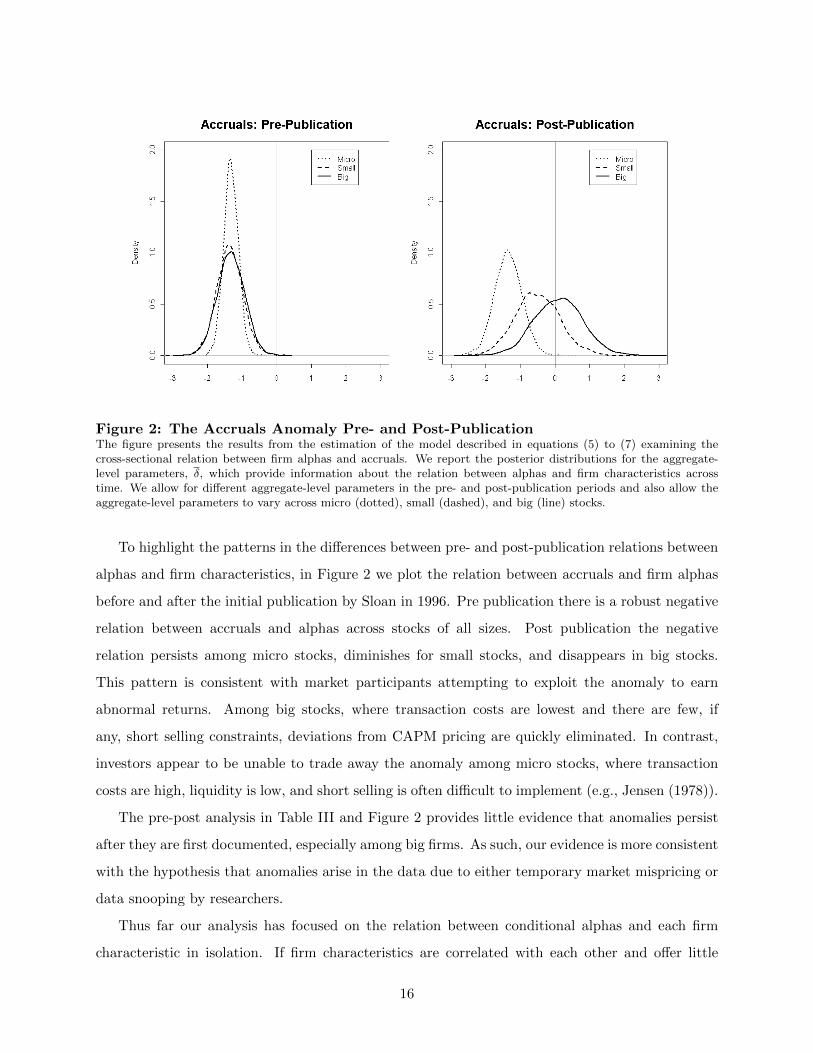
Figure 2: The Accruals Anomaly Pre- and Post-PublicationThe figure presents the results from the estimation of the model described in equations (5) to (7) examining thecross-sectional relation between firm alphas and accruals. We report the posterior distributions for the aggregate-level parameters, δ, which provide information about the relation between alphas and firm characteristics acrosstime. We allow for different aggregate-level parameters in the pre- and post-publication periods and also allow theaggregate-level parameters to vary across micro (dotted), small (dashed), and big (line) stocks.

To highlight the patterns in the differences between pre- and post-publication relations between

alphas and firm characteristics, in Figure 2 we plot the relation between accruals and firm alphas

before and after the initial publication by Sloan in 1996. Pre publication there is a robust negative

relation between accruals and alphas across stocks of all sizes. Post publication the negative

relation persists among micro stocks, diminishes for small stocks, and disappears in big stocks.

This pattern is consistent with market participants attempting to exploit the anomaly to earn

abnormal returns. Among big stocks, where transaction costs are lowest and there are few, if

any, short selling constraints, deviations from CAPM pricing are quickly eliminated. In contrast,

investors appear to be unable to trade away the anomaly among micro stocks, where transaction

costs are high, liquidity is low, and short selling is often difficult to implement (e.g., Jensen (1978)).

The pre-post analysis in Table III and Figure 2 provides little evidence that anomalies persist

after they are first documented, especially among big firms. As such, our evidence is more consistent

with the hypothesis that anomalies arise in the data due to either temporary market mispricing or

data snooping by researchers.

Thus far our analysis has focused on the relation between conditional alphas and each firm

characteristic in isolation. If firm characteristics are correlated with each other and offer little

16

Figure 3: Individual and Multiple Anomaly VariablesThe figure presents the results from the estimation of the model described in equations (5) to (7) examining thecross-sectional relation between firm alphas and multiple firm characteristics simultaneously. We report the posteriordistributions (line) for the aggregate-level parameters, δ, which provide information about the relation between alphasand firm characteristics across the entire sample period. For comparison, for each anomaly variable we also presentthe posterior distribution (dashed) of δ from estimation of the model described in equations (5) to (7) for eachcharacteristic in isolation using the same data sample.

unique information about alphas then studying each characteristic in isolation will overstate the

failings of the conditional CAPM. The traditional portfolio approach is unable to adequately address

this omitted variable problem. Researchers typically rely on two- or possibly three-way sorts to

isolate the effects of a particular characteristic. Controlling for more than one or two characteristics

simultaneously, however, is infeasible, and inferences are sensitive to both the sorting technique

and the sorting sequence (e.g., Conrad, Cooper, and Kaul (2003)). In contrast, our approach is

particularly well suited to assess which anomalies contain unique information; we simply specify

firm-year alphas in equation (6) as a function of all nine firm characteristics from Table I.

In Figure 3 we compare the posterior distributions from two analyses – one in which each

firm characteristic is considered in isolation and one in which all characteristics are considered

simultaneously. Momentum, asset growth, and financial distress are significantly associated with

CAPM alphas when considered in isolation, but as Figure 3 highlights, none of these characteristics

contain significant incremental information when all firm characteristics are considered simultane-

ously. The only firm characteristics that are significantly related to firm-level alphas when multiple

characteristics are considered simultaneously are book-to-market, profitability, net stock issues,

17

and accruals.15 Our analysis therefore suggests that univariate tests provide a low hurdle for firm

characteristics to be classified as anomalies.

5 Conclusion

In this paper, we develop a hierarchical Bayes model to examine asset-pricing anomalies, model-

ing firm-year alphas as a function of one or more firm characteristics. We investigate nine anomalies

– size, book-to-market, momentum, reversal, profitability, asset growth, net stock issues, accruals,

and financial distress – over the period 1963 to 2008. Studying each anomaly separately we find

robust evidence that conditional CAPM alphas are positively associated with book-to-market, mo-

mentum, and profitability, and negatively associated with asset growth, net stock issues, accruals,

and financial distress.

These initial results imply the failings of the CAPM are widespread. A deeper investigation

of anomalies, however, suggests that while the CAPM may not perfectly explain firm returns,

the anomaly-based evidence against the CAPM is greatly overstated. Relations between firm

characteristics and conditional firm-level alphas are primarily confined to micro and small stocks

and tend not to persist after the anomalies are first documented. Furthermore, few of the firm

characteristics associated with alphas actually contain unique information.

15In results not reported we also considered a model specification in which conditional alphas were modeled as afunction of multiple firm characteristics and the relations were allowed to vary across micro, small, and big stocks.As in Figure 1 the relations between characteristics and alphas are generally driven by micro and small stocks.

18

A Model Appendix

Section A.1 provides details about the MCMC estimation algorithm, and Section A.2 presents

a simulation study that demonstrates the ability of the algorithm to accurately recover parameters.

A.1 Estimation Methodology

The model outlined in equations (5) to (7) can be estimated by repeatedly cycling through

steps 1 to 6 below. As discussed in the text, we place a hierarchical structure on alphas, but not

on betas. Instead we impose a proper, but diffuse, prior directly on betas in the base specification,

βi,y ∼ N (1, 10). Let ri,t,y denote the excess return on stock i in month t of year y and rm,t,y the

excess return on the market portfolio. Further, let Zy denote a matrix in which the first column is

a vector of ones and the second column is the excess returns on the market portfolio, and let Xy

denote a matrix of a constant and firm-year characteristics associated with anomalies.

1. Draw αi,y, βi,y|σ2i,y, δy, σ2α,y for each stock i = 1, ..., N , in each year y = 1, ..., Y . We obtain a

draw from the marginal posterior distribution of αi,y and βi,y as follows:

αi,y

βi,y

∼ N (λi, (σ−2i,y Z ′yZy + V−1λ )−1), (A.1)

where

λi = (σ−2i,y Z′yZy + V−1λ )−1(σ−2i,y Z

′yZyλ̂i + V−1λ λi,y), (A.2)

λ̂i =(Z ′yZy

)−1Z ′yri,y, (A.3)

λi,y =

Xi,yδy

1

, (A.4)

and

Vλ =

σ2α,y 0

0 10

. (A.5)

2. Draw σ2i,y |αi,y, βi,y for each stock i = 1, ..., N , in each year y = 1, ..., Y . We obtain a draw

from the marginal posterior distribution of σ2i,y as follows:

σ2i,y ∼ Inverse Gamma

(v1s

21

2,v12

), (A.6)

19

v1 = v0 +M, (A.7)

and

s21 =v0s

20 + s2

v0 +M, (A.8)

where s2 is the sample sum of squared errors and M denotes the number of observations.

The priors, v0 and s20, are determined by the researcher. We set v0 equal to 3 and s20 equal

to the variance of the monthly returns for stock i in year y.

3. Draw δy| {αi,y} , σ2α,y, δ,V for each year y = 1, ..., Y . Let αy denote a column vector composed

of draws of αi,y for all firms i in the dataset in year y. We obtain a draw from the marginal

posterior distribution of δy as follows:

δy ∼ N(δy, (σ

−2α,yX

′yXy + V−1)−1

), (A.9)

where

δy = (σ−2α,yX′yXy + V−1)−1(σ−2α,yX

′yXy δ̂y + V−1δ), (A.10)

and

δ̂y =(X ′yXy

)−1X ′yαy. (A.11)

4. Draw σ2α,y | {αi,y} , δy for each year y = 1, ..., Y . We obtain a draw from the marginal posterior

distribution of σ2α,y as follows:

σ2α,y ∼ Inverse Gamma

(v1s

21

2,v12

), (A.12)

v1 = v0 +M, (A.13)

and

s21 =v0s

20 + s2

v0 +M, (A.14)

where s2 is the sample sum of squared errors and M denotes the number of observations. The

priors, v0 and s20, are determined by the researcher. We set v0 equal to 3. We elicit priors for

s20 in the following manner. For each stock in year y we estimate equation (5) using OLS and

store α̂. We set s20 equal to the variance of α̂ across all firms in year y.

20

Having drawn the firm- and year-level coefficients we proceed to draw the aggregate-level pa-

rameters. Let P denote a Y ×nvar matrix comprised of a draw of {δy}Yy=1 , where nvar denotes the

number of columns in X, and let H be a matrix of covariates the researcher believes to be associated

with the evolution of the parameter vector δy over time. In our specification, H is a column vector

of ones, but could easily be extended, for example, to include macroeconomic variables.

5. Draw V| {δy}. We obtain a draw from the marginal posterior distribution of V as follows:

V ∼ Inverse Wishart (nvar +Nu+ Y,V0 + S) , (A.15)

where

S =(P −HΓ̃

)′ (P −HΓ̃

)+(Γ̃− Γ

)′A(Γ̃− Γ

), (A.16)

Γ̃ =((H ′H + A

)−1 (H ′HΓ̂ + AΓ

)), (A.17)

and

Γ̂ =(H ′H

)−1 (H ′P

). (A.18)

A, Γ, Nu and V0 are priors specified by the researcher. We set A−1 = 100I and define Γ to

be an nH × nvar matrix of zeros, where nH denotes the number of columns in H. Nu is set

to nvar + 3, and V0 = NuI. I denotes an appropriately dimensioned identity matrix.

6. Draw γ| {δy} ,V. We obtain a draw from the marginal posterior distribution of γ as follows:

γ ∼ N(γ̃,V ⊗

(H ′H + A

)−1), (A.19)

where γ̃ = vec(Γ̃). Given that H is a vector of ones, δ = γ.

A.2 Model Simulation

In this section, we conduct a simulation exercise and show our estimation algorithm successfully

recovers the parameters of interest. Data are created for 1,000 firms over a 45-year period. The

length of each time period, y, is set to 12 months. We assume there are two firm characteristics

associated with firm-level alphas, x1 and x2, which are both uniformly distributed over the range

-0.5 to +0.5. The parameters in the simulation are set to ensure that the simulated firm-level

returns, alphas, betas, and market returns are consistent with the actual values observed using the

21

CRSP return data.

1. Draw δy ∼ MVN(µ = δ, σ2 = V

)for each 12-month time period, y. We set

δ =

δ0 = 0

δ1 = 1

δ2 = 1

, and V =

1.5 0.5 0.5

0.5 1.5 0.5

0.5 0.5 1.5

.2. Draw αy ∼ MVN

(µ = δ0,y + δ1,yx1 + δ2,yx2, σ

2 = Σα

), where αy is a column vectors of firm-

specific alphas in time period y. We consider two specifications for the variance-covariance

matrix, Σα, one in which the error terms are independent across firms, and one in which the

error terms are correlated across firms. We examine two different levels of correlations, low to

medium with correlations ranging from −0.5 to +0.5, and medium to high with correlations

ranging from −0.9 to +0.9. The diagonal elements of Σα are set equal to σ2α = 2.16

3. Draw βi,y ∼ N(µ = 1, σ2 = 4

)for each firm i in each time period y.

4. Generate excess monthly returns on the market: rm,t,y ∼ N(µ = 0.5, σ2 = 25

).

5. Generate monthly excess returns for each firm in each month of each time period: rt,y =

αy + βyrm,t,y + εt,y, where εt,y ∼ MVN(µ = 0, σ2 = Σret

)and rt,y denotes a column vector

of excess returns for all firms in month t of time period y. αy and βy are column vectors of

firm-specific alphas and betas. The specifications for the variance-covariance matrix, Σret,

are constructed in a similar manner to those for Σα. The only difference is that the diagonal

elements of Σret, σ2ret, are set equal to 169.

We examine seven different scenarios to investigate the sensitivity of our model to different

correlation structures in the error terms of equations (5) and (6). The MCMC algorithm is run

for 1,000 iterations for each scenario. The algorithm converges quickly. The posterior distributions

are characterized using the final 500 iterations. We use the same seed for the random number

generator for each scenario. Table A.I reports the results from the simulation study. Regardless

of the correlation structure in the error terms of equations (5) and (6), the estimation algorithm

16We use the following procedure to create a 1,000 × 1,000 variance-covariance matrix. First, create a columnvector, u, with 1,000 draws from the Uniform(-1,1) distribution. Second, calculate κuu′ where κ = pσ2

α. Theparameter, p is a scaling factor, between 0 and 1, for the maximum level of correlation in the error terms across firms.If p = 0, firm-level alphas are independent. If p = 1, κuu′ correlations range from −1 to +1. For low to mediumcorrelations we set p = 0.5, while for medium to high correlations we set p = 0.9. Finally, set Σα = κuu′ and replacethe diagonal elements with σ2

α = 2.

22

is able to accurately recover the aggregate-level model parameters, δ and V, indicating that the

approach is not sensitive to the possibility of cross-correlations across firms.

23

Tab

leA

.I:

Mod

el

Est

imati

on

on

Sim

ula

ted

Data

.T

he

table

pre

sents

the

resu

lts

from

the

esti

mati

on

of

the

model

des

crib

edin

equati

ons

(5)

to(7

)fo

rsi

mula

ted

data

.W

ere

port

the

post

erio

rm

ean

and

standard

dev

iati

on

for

the

aggre

gate

-lev

elpara

met

ersδ

and

V.

We

sim

ula

tedata

for

1,0

00

firm

sov

era

45-y

ear

per

iod.

We

esti

mate

the

model

usi

ng

annual

per

iods

and

month

lysu

bp

erio

ds.

We

crea

tese

ven

diff

eren

tse

tsof

data

usi

ng

the

sam

ese

edfo

rth

era

ndom

num

ber

gen

erato

rin

each

scen

ari

o.

Each

set

of

data

diff

ers

only

wit

hre

spec

tto

the

ass

um

pti

ons

ab

out

cross

-corr

elati

ons

inth

eer

ror

term

sof

equati

on

(5)

(month

lyfirm

retu

rns)

and/or

equati

on

(6)

(firm

-yea

ralp

has)

.Sp

ecifi

cally,

we

allow

cross

-corr

elati

ons

inea

cheq

uati

on

tota

ke

on

one

of

thre

ele

vel

s:ze

ro,

low

,or

hig

h.

The

low

level

allow

scr

oss

-corr

elati

ons

tora

nge

bet

wee

n∓

0.5

,w

hile

the

hig

hle

vel

allow

scr

oss

-corr

elati

ons

tora

nge

bet

wee

n∓

0.9

.W

eru

nth

eG

ibbs

sam

ple

rfo

r1,0

00

iter

ati

ons

and

dis

card

the

firs

t500

as

aburn

-in

per

iod.

An∗

(∗∗)

indic

ate

sth

at

the

95%

(99%

)cr

edib

lein

terv

al

of

the

post

erio

rdis

trib

uti

on

does

not

incl

ude

the

true

valu

e.

Cro

ss-C

orr

elati

on

Cro

ss-C

orr

elati

on

inR

eturn

Err

or

inA

lpha

Err

or

Case

(Equati

on

(5))

(Equati

on

(6))

δ 0δ 1

δ 2V

11

V22

V33

V12

V13

V23

Tru

eV

alu

es0.0

01.0

01.0

01.5

01.5

01.5

00.5

00.5

00.5

0

Post

erio

rM

eans

for

the

Aggre

gate

-Lev

elP

ara

met

ers,δ

and

V

Case

1N

one

None

-0.2

20.9

41.0

71.8

61.7

41.6

70.5

70.6

80.7

5(0

.20)

(0.2

0)

(0.2

1)

(0.3

9)

(0.3

8)

(0.4

0)

(0.2

9)

(0.3

1)

(0.2

8)

Case

2L

owN

one

-0.2

10.8

71.0

61.8

61.7

91.6

50.5

10.6

70.7

8(0

.20)

(0.2

0)

(0.2

1)

(0.3

9)

(0.3

9)

(0.4

0)

(0.2

9)

(0.3

1)

(0.2

9)

Case

3H

igh

None

-0.2

00.8

41.0

81.8

71.7

91.6

50.4

90.6

60.7

8(0

.20)

(0.2

0)

(0.2

1)

(0.3

9)

(0.3

9)

(0.4

0)

(0.2

9)

(0.3

1)

(0.2

9)

Case

4N

one

Low

-0.2

20.9

31.0

71.8

61.7

41.7

20.5

60.6

80.7

9(0

.20)

(0.2

0)

(0.2

1)

(0.3

9)

(0.3

8)

(0.4

1)

(0.2

9)

(0.3

1)

(0.2

9)

Case

5N

one

Hig

h-0

.22

0.9

31.0

71.8

61.7

41.7

20.5

60.6

70.8

0(0

.20)

(0.2

0)

(0.2

1)

(0.3

9)

(0.3

8)

(0.4

1)

(0.2

9)

(0.3

1)

(0.2

9)

Case

6L

owL

ow-0

.21

0.8

61.0

61.8

61.8

21.7

00.5

10.6

60.8

2(0

.20)

(0.2

0)

(0.2

1)

(0.3

9)

(0.4

0)

(0.4

1)

(0.3

0)

(0.3

1)

(0.3

0)

Case

7H

igh

Hig

h-0

.20

0.8

31.0

81.8

81.8

21.6

90.4

90.6

40.8

4(0

.20)

(0.2

0)

(0.2

1)

(0.3

9)

(0.4

0)

(0.4

1)

(0.3

0)

(0.3

1)

(0.3

0)

24

B Data Appendix

We obtain accounting data from the Compustat Fundamentals Annual files and stock return

data from the CRSP monthly return files. Each of the anomaly variables is measured once a year at

the end of June in calendar year y. The variables are matched to returns from July of calendar year

y to June of calendar year y+1. To ensure that the accounting data are known prior to the returns

they are used to forecast, we lag all accounting variables by six months. The sample includes all

NYSE, Amex, and NASDAQ ordinary common stocks with the data required to compute at least

one of the following anomaly variables:

1. M (Size): The natural log of price per share times the number of shares outstanding at the

end of June of year y.

2. BM (Book-to-market): The natural log of the ratio of book value of equity to market value

of equity. Following Fama and French (2008), we define the book value of equity as total

assets (at), minus total liabilities (lt), plus balance sheet deferred taxes and investment tax

credits (txditc) if available, minus the book value of preferred stock if available. Depending

on availability, we use liquidating value (pstkl), redemption value (pstkrv), or carrying value

(upstk) for the the book value of preferred stock. The market value of equity is price per

share times the number of shares outstanding at the end of December of year y − 1.

3. MOM (Momentum): The continuously compounded stock return from January to June of

year y. We require a firm to have a price for the end of December of year y − 1 and a good

return for June of year y.

4. REV (Reversal): The continuously compounded stock return from July of year y−5 to June

of year y − 1. We require a firm to have a price for the end of June of year y − 5 and a good

return for June of year y − 1.

5. ROA (Profitability): Income before extraordinary items (ib), minus dividends on preferred

(dvp) if available, plus income statement deferred taxes (txdi) if available divided by total

assets (at).

6. AG (Asset growth): Total assets (at) at the fiscal year end in year y − 1, minus total assets

at the fiscal year end in year y− 2 divided by total assets at the fiscal year end in year y− 2.

We also require a firm to have non-zero total assets in both year y − 1 and y − 2.

25

7. NS (Net stock issues): The natural log of the ratio of split-adjusted shares at the fiscal year

end in year y − 1 divided by split-adjusted shares at the fiscal year end in year y − 2. The

number of split-adjusted shares outstanding is common shares outstanding from Compustat

(csho) times the cumulative adjustment factor by ex-date (adjex f).

8. ACC (Accruals): The change in current assets (act) from the fiscal year end in year y− 2 to

y − 1, minus the change in current liabilities (lct), minus the change in cash and short-term

investments (che), plus the change in debt in current liabilities (dlc), minus depreciation (dp)

in fiscal year y − 1 divided by total assets (at) from the fiscal year end in year y − 2.

9. OS (Financial distress): Ohlson’s (1980) O-score:

O-score =1

1 + exp(−x),

where

x =− 1.32− 0.407 (SIZE) + 6.03 (TLTA)− 1.43 (WCTA)

+ 0.076 (CLCA)− 1.72 (OENEG)− 2.37 (NITA)− 1.83 (FUTL)

+ 0.285 (INTWO)− 0.521 (CHIN) ,

where SIZE is the log of the ratio of total assets (at) to the GNP price-level index, TLTA

is the ratio of total liabilities (lt) to total assets, WCTA is the ratio of working capital (act

– lct) to total assets, CLCA is the ratio of current liabilities (lct) to current assets (act),

OENEG is a dummy variable equal to one if total liabilities exceeds total assets and zero

otherwise, NITA is the ratio of net income (ni) to total assets, FUTL is the ratio of funds

from operations (pi) to total liabilities, INTWO is a dummy variable equal to one if total

net income was negative for the past two years and zero otherwise, and CHIN is the change

in net income from fiscal year y − 2 to y − 1 divided by the sum of the absolute values of

net income in fiscal years y − 2 and y − 1. Data on the GNP price-level index are from the

Federal Reserve Bank of St. Louis website.17 Following Ohlson (1980), we assign the index

a value of 100 in 1968, and the index year is as of the year prior to the year of the balance

sheet date.

17http://research.stlouisfed.org/fred2/.

26

We exclude financial firms (SIC codes between 6000 and 6999) and firms with negative book

equity. The sample period is July 1963 to June 2008. To alleviate the influence of outliers, we

winsorize ROA, AG, NS, and ACC at the 1st and 99th percentiles. For cases in which a firm is

delisted from an exchange during a given month, we replace any missing returns with the delisting

returns provided by CRSP.

27

References

Ahn, Dong-Hyun, Jennifer Conrad, and Robert F. Dittmar, 2009, Basis assets, Review of FinancialStudies 22, 5133–5174.

Ang, Andrew, and Joseph Chen, 2007, CAPM over the long run: 1926–2001, Journal of EmpiricalFinance 14, 1–40.

Ang, Andrew, Jun Liu, and Krista Schwarz, 2010, Using stocks or portfolios in tests of factormodels, Working paper, Columbia University.

Avramov, Doron, and Tarun Chordia, 2006, Asset pricing models and financial market anomalies,Review of Financial Studies 19, 1001–1040.

Banz, Rolf W., 1981, The relationship between return and market value of common stocks, Journalof Financial Economics 9, 3–18.

Brennan, Michael J., Tarun Chordia, and Avanidhar Subrahmanyam, 1998, Alternative factorspecifications, security characteristics, and the cross-section of expected stock returns, Journalof Financial Economics 49, 345–373.

Campbell, John Y., Jens Hilscher, and Jan Szilagyi, 2008, In search of distress risk, Journal ofFinance 63, 2899–2939.

Chan, Louis K.C., Yasushi Hamao, and Josef Lakonishok, 1991, Fundamentals and stock returnsin Japan, Journal of Finance 46, 1739–1764.

Chava, Sudheer, and Amiyatosh K. Purnanandam, 2010, Is default risk negatively related to stockreturns?, Review of Financial Studies 23, 2523–2559.

Chopra, Navin, Josef Lakonishok, and Jay R. Ritter, 1992, Measuring abnormal performance: Dostocks overreact?, Journal of Financial Economics 31, 235–268.

Cohen, Randolph B., Paul A. Gompers, and Tuomo Vuolteenaho, 2002, Who underreacts to cash-flow news? Evidence from trading between individuals and institutions, Journal of FinancialEconomics 66, 409–462.

Collins, Daniel W., and Paul Hribar, 2000, Earnings-based and accrual-based market anomalies:One effect or two?, Journal of Accounting and Economics 29, 101–123.

Conrad, Jennifer, Michael Cooper, and Gautam Kaul, 2003, Value versus glamour, Journal ofFinance 58, 1969–1996.

Cooper, Michael J., Huseyin Gulen, and Michael J. Schill, 2008, Asset growth and the cross-sectionof stock returns, Journal of Finance 63, 1609–1651.

Cremers, K. J. Martijn, 2006, Multifactor efficiency and Bayesian inference, Journal of Business79, 2951–2998.

Daniel, Kent, and Sheridan Titman, 2006a, Market reactions to tangible and intangible information,Journal of Finance 61, 1605–1643.

, 2006b, Testing factor-model explanations of market anomalies, Working paper, North-western University.

28

DeBondt, Werner F. M., and Richard Thaler, 1985, Does the stock market overreact?, Journal ofFinance 40, 793–805.

Dichev, Ilia D., 1998, Is the risk of bankruptcy a systematic risk?, Journal of Finance 53, 1131–1147.

Dimson, Elroy, 1979, Risk measurement when shares are subject to infrequent trading, Journal ofFinancial Economics 7, 197–226.

Fairfield, Patricia M., J. Scott Whisenant, and Teri Lombardi Yohn, 2003, Accrued earnings andgrowth: Implications for future profitability and market mispricing, The Accounting Review 78,353–371.

Fama, Eugene F., and Kenneth R. French, 1992, The cross-section of expected stock returns,Journal of Finance 47, 427–465.

, 2006, The value premium and the CAPM, Journal of Finance 61, 2163–2185.

, 2008, Dissecting anomalies, Journal of Finance 63, 1653–1678.

Geweke, John, and Guofu Zhou, 1996, Measuring the pricing error of the Arbitrage Pricing Theory,Review of Financial Studies 9, 557–587.

Gomes, Joao, Leonid Kogan, and Lu Zhang, 2003, Equilibrium cross section of returns, Journal ofPolitical Economy 111, 693–732.

Harvey, Campbell R., 1989, Time-varying conditional covariances in tests of asset pricing models,Journal of Financial Economics 25, 289–317.

Harvey, Campbell R., and Guofu Zhou, 1990, Bayesian inference in asset pricing tests, Journal ofFinancial Economics 26, 221–254.

Haugen, Robert A., and Nardin L. Baker, 1996, Commonality in the determinants of expectedstock returns, Journal of Financial Economics 41, 401–439.

Ikenberry, David, Josef Lakonishok, and Theo Vermaelen, 1995, Market underreaction to openmarket share repurchases, Journal of Financial Economics 39, 181–208.

Jagannathan, Ravi, and Zhenyu Wang, 1996, The conditional CAPM and the cross-section ofexpected returns, Journal of Finance 51, 3–53.

Jegadeesh, Narasimhan, 1990, Evidence of predictable behavior of security returns, Journal ofFinance 45, 881–898.

Jegadeesh, Narasimhan, and Sheridan Titman, 1993, Returns to buying winners and selling losers:Implications for stock market efficiency, Journal of Finance 48, 65–91.

, 2001, Profitability of momentum strategies: An evaluation of alternative explanations,Journal of Finance 56, 699–720.

Jensen, Michael C., 1978, Some anomalous evidence regarding market efficiency, Journal of Finan-cial Economics 6, 95–102.

Kan, Raymond, 2004, On the explanatory power of asset pricing models across and within portfolios,Working paper, University of Toronto.

29

Kandel, Shmuel, Robert McCulloch, and Robert F. Stambaugh, 1995, Bayesian inference andportfolio efficiency, Review of Financial Studies 8, 1–53.

Kandel, Shmuel, and Robert F. Stambaugh, 1995, Portfolio inefficiency and the cross section ofexpected returns, Journal of Finance 50, 157–184.

Karolyi, G. Andrew, 1992, Predicting risk: Some new generalizations, Management Science 38,57–74.

Lettau, Martin, and Sydney Ludvigson, 2001, Resurrecting the (C)CAPM: A cross-sectional testwhen risk premia are time-varying, Journal of Political Economy 109, 1238–1287.

Lewellen, Jonathan, and Stefan Nagel, 2006, The conditional CAPM does not explain asset-pricinganomalies, Journal of Financial Economics 82, 289–314.

Lewellen, Jonathan, Stefan Nagel, and Jay Shanken, 2010, A skeptical appraisal of asset-pricingtests, Journal of Financial Economics 96, 175–194.

Lintner, John, 1965, The valuation of risk assets and the selection of risky investments in stockportfolios and capital budgets, Review of Economics and Statistics 47, 13–37.

Litzenberger, Robert H., and Krishna Ramaswamy, 1979, The effect of personal taxes and dividendson capital asset prices: Theory and empirical evidence, Journal of Financial Economics 7, 163–195.

Lo, Andrew W., and A. Craig MacKinlay, 1990, Data-snooping biases in tests of financial assetpricing models, Review of Financial Studies 3, 431–468.

Loughran, Tim, 1997, Book-to-market across firm size, exchange, and seasonality, Journal of Fi-nancial and Quantitative Analysis 32, 249–268.

Loughran, Tim, and Jay R. Ritter, 1995, The new issues puzzle, Journal of Finance 50, 23–51.

McCulloch, Robert, and Peter E. Rossi, 1991, A Bayesian approach to testing the Arbitrage PricingTheory, Journal of Econometrics 49, 141–168.

Ohlson, James A., 1980, Financial ratios and the probabilistic prediction of bankruptcy, Journalof Accounting Research 18, 109–131.

Pontiff, Jeffrey, and Artemiza Woodgate, 2008, Share issuance and cross-sectional returns, Journalof Finance 63, 921–945.

Roll, Richard, 1977, A critique of the asset pricing theory’s tests – Part I: On past and potentialtestability of the theory, Journal of Financial Economics 4, 129–176.

Rosenberg, Barr, Kenneth Reid, and Ronald Lanstein, 1985, Persuasive evidence of market ineffi-ciency, Journal of Portfolio Management 11, 9–17.

Rossi, Peter E., Greg M. Allenby, and Rob McCulloch, 2005, Bayesian Statistics and Marketing.John Wiley & Sons, West Sussex, England.

Schwert, G. William, 2003, Anomalies and market efficiency, in George M. Constantinides, MiltonHarris, and Rene M. Stulz, eds.: Handbook of the Economics of Finance (North Holland).

30

Shanken, Jay, 1987, A Bayesian approach to testing portfolio efficiency, Journal of Financial Eco-nomics 19, 195–215.

Shanken, Jay, and Guofu Zhou, 2007, Estimating and testing beta pricing models: Alternativemethods and their performance in simulations, Journal of Financial Economics 84, 40–86.

Shanken, Jay A., 1990, Intertemporal asset pricing: An empirical investigation, Journal of Econo-metrics 45, 99–120.

Sharpe, William F., 1964, Capital asset prices: A theory of market equilibrium under conditionsof risk, Journal of Finance 19, 425–442.

Sloan, Richard G., 1996, Do stock prices fully reflect information in accruals and cash flows aboutfuture earnings?, The Accounting Review 71, 289–315.

Titman, Sheridan, K. C. John Wei, and Feixue Xie, 2004, Capital investments and stock returns,Journal of Financial and Quantitative Analysis 39, 677–700.

Vasicek, Oldrich A., 1973, A note on using cross-sectional information in Bayesian estimation ofsecurity betas, Journal of Finance 28, 1233–1239.

Xie, Hong, 2001, The mispricing of abnormal accruals, The Accounting Review 76, 357–373.

31