Asset Allocation Models and Market Volatility

Eric Jacquiera

Alan J. Marcusb

Forthcoming Financial Analyst Journal

October 2000

a Assistant Professor of Finance, Finance Department, Carroll School of Management,Boston College, Chestnut Hill, MA 02467. Invited Researcher CIRANO Montreal(www.cirano.umontreal.ca). Tel: (617) 552-2943, Email: jacquier@jacquier.bc.edu,Web: www2.bc.edu/~jacquier

b Professor of Finance, Finance Department, Carroll School of Management, BostonCollege, Chestnut Hill, MA 02467. Tel: (617) 552-2767, Email: alan.marcus@bc.edu

Abstract

While asset allocation and risk management models all assume at least short-term

stability of the covariance structure of asset returns, actual covariance and correlation

relationships vary wildly, even over short horizons. Moreover, correlations increase in

volatile periods, reducing the power of diversification when it might most be desired. We

attempt to explain these phenomena and to present a framework for predicting short-

horizon changes in correlation structure. We model correlations across assets as due to

the common dependence of returns on a market-wide, systematic factor. Through this

link, an increase in factor volatility increases the relative importance of systematic risk

compared to the unsystematic component of returns. This in turn results in an increase in

asset correlations.

We find that a very large fraction of the time-variation in cross-industry

correlation can be explained solely by variation in the volatility of the market index.

Moreover, there is enough predictability in index volatility to allow us to construct useful

forecasts of covariance matrices in coming periods. Cross-country correlations behave in

a qualitatively similar manner, but country-specific residuals are more pronounced than

industry residuals, which reduces the efficacy of our approach.

Asset allocation and efficient diversification are at the heart of portfolio theory,

and asset correlation structure is at the heart of efficient diversification. When that

structure may be treated as stable over an investment horizon, the portfolio construction

problem is well understood. In recent years, moreover, it has become clear that portfolio

theory is also crucial to risk management. The risk manager uses the covariance matrix

to compute probabilities of extreme outcomes or to minimize the risk of a portfolio of

positions.

However, there is ample evidence that correlation and covariance structures vary

dramatically over time, so much so and with such high frequency, that one must wonder

whether asset allocation and risk management models can be of any use whatsoever. To

illustrate the variation in correlation across U.S. industry groups, we use daily returns to

calculate the correlation matrix of 12 industries for each quarter between 1962:3 and

1997:4. (See Table 1 for a description of the 12 industries.) Figure 1, Panel A presents

box plots of the 12×11/2 = 66 cross-industry correlations for each quarter. The dramatic

and unpredictable shifts in correlation structure over time suggest the difficulties one

might encounter when attempting to use mean-variance analysis assuming a stable

correlation structure. Instability seems to characterize international correlation structure

as well. Figure 1, Panel B, shows analogous box plots for correlations of equity index

returns across ten countries.1 The same instability is evident.

1 The 10 countries are the U.S., U.K., Japan, France, Germany, Hong Kong, Canada, Australia,

Switzerland, and Belgium. The returns are dollar-denominated, thus measuring the performance of each

index from the perspective of an unhedged U.S. investor.

-2-

Moreover, correlation structure varies over time in ways that to a portfolio or risk

manager must seem perverse. For example, it is well-documented that cross-country

correlations increase markedly during periods of high global market volatility [see for

example, Chow et al. (1999), Longin and Solnik (1995) or Solnik, Foucrelle, and Le Fur

(1996)]. This means that the power of diversification is weakest precisely when it would

be most desired. This phenomenon is often called correlation breakdown. While not as

widely discussed, this pattern is, if anything, even more characteristic of cross-industry

correlations in a domestic context.

Figures 2a and 2b illustrate this phenomenon in our data. The variation in cross-

industry correlation is highly associated with market volatility. In Figure 2, Panel A, we

plot the median of the 66 cross-correlations between industry sectors for each quarter

against the volatility of the S&P 500 index computed from the daily returns of the S&P

500 in the same quarter.2 Panel B presents the same plot of median cross-country

correlation as a function of the standard deviation of the MSCI-World equity index in that

quarter. In both contexts, correlation clearly rises with volatility. Correlation breakdown

is obvious and dramatic.

These empirical patterns raise two questions. First, what drives such variation in

correlation structure, and second, can we devise simple models of correlation/covariance

2 The actual relationship between correlation and market volatility is non-linear. This is not surprising for a

plot of correlation coefficients (which are bounded between −1 and 1) against volatility, which must be

positive. Therefore, in Figure 2, we plot the relationship using a common transformation of the data.

Calling ρ the correlation coefficient, and σM the standard deviation of the index return, the vertical axis is

ln(1 + ρ1 − ρ) , and the horizontal axis is log(σM), both of which have a range of (−∞, +∞). The transformed

relationship is apparently linear, and obviously strong.

-3-

structure that account for and predict such variation to an extent that is useful to a risk

manager.

Our basic insight in this paper derives from a simple observation: Correlations

will be higher when systematic macroeconomic factors, which affect all assets in tandem,

dominate sector-specific factors. If variations in asset returns are driven by both

systematic factors and idiosyncratic (i.e., sector-specific) risks, then periods of high

factor volatility will coincide with periods of high correlation: during these periods, the

dominant source of variation will be due to the common factor. Unless idiosyncratic

volatility is strongly correlated across sectors (which is not the case in our sample),

periods of high cross-sector correlation will coincide with periods of high overall market

volatility. Thus, correlation breakdown − the strong observed association between

correlation and volatility − is not simply bad luck. It is to be expected. Moreover, it is

not evidence that the structure of security returns periodically changes perversely;

“breakdown” can be part and parcel of a stable factor model of returns.

Moreover, this argument suggests that risk managers can use simple factor models

of portfolio returns to better understand and predict time-variation in correlation.3 In all

3 Not surprisingly, factor models have been used and studied extensively. The most relevant test

of such models for our purposes is Chan, Karceski, and Lakonishok (1999), who find that correlations

derived from a three-factor model (with factors equal to the return on a value-weighted market index, and

returns on size and book-to-market portfolios) are as effective as larger factor models in predicting

covariance or correlation and managing portfolio risk, and in fact that none of the multi-factor models offer

dramatic improvement in risk control compared to the one-factor market model. Our focus differs from

theirs in several ways, however. Whereas CKL estimate models that predict unconditional covariances, we

are more concerned with the conditional relationship between correlation and overall market volatility. As

-4-

of these models, correlation across sectors is due to their common dependence on shocks

to systematic factors, and changes in correlation are driven by changes in the volatility of

those shocks. During periods of large macroeconomic disturbances, the common factor

dominates the volatility of individual sector returns, and leads to higher correlations. In

quieter periods, sector-specific risks might dominate, with the results that correlations are

lower and diversification eliminates a greater fraction of total volatility.

We find that a simple univariate factor model with only one systematic factor can

explain a surprisingly large fraction of the short-horizon time variation in correlation

structure. This suggests that univariate models of time variation in volatility, such as the

ARCH model and its variants, which are already widely and successfully applied, can be

integrated with the factor model to make useful short-horizon forecasts of cross-sector

correlations. We find that short-term variation across time in the volatility of the "macro

factor" can be used to forecast most of the time variation in correlation, and thus guide

managers in dynamically updating portfolio positions. The results are qualitatively the

same in the international and domestic settings. However, there is considerably more

country-specific volatility than industry-specific volatility, implying that while the

proposed methodology can be quite effective in the domestic setting, it will be less useful

in the international setting.

The paper is organized as follows. In the next section, we briefly review the

index model that serves to organize our approach. In Section 2, we examine the relation

between correlation structure and market volatility for domestic portfolios, and examine

a result, while monthly data is appropriate for the tests in CKL, we use higher frequency daily data that

allows us to focus on shorter-term variation in market and asset volatility.

-5-

the contribution of variation in factor volatility to the time variation in correlation

structure. We find that factor volatility almost solely determines the variation in

correlation structure. We use this result to propose simple estimators of covariance

matrices even for a large number of asset classes, and document the out-of-sample

performance of this model. We find that models using only variation in volatility to

predict changes in correlation perform extremely well. In Section 3, we present a parallel

analysis for international asset classes. These results are qualitatively the same as in the

domestic setting, but the higher level of country-specific risk makes the approach less

effective. For international equity portfolios, factor volatility is important, but is not

nearly as single-handedly determinative. The last section concludes.

1. THE INDEX MODEL

Sharpe (1963) was the first to show that an index model could potentially simplify

the portfolio construction problem. His approach has become the textbook model for

portfolio construction (literally – see for example, Bodie, Kane, Marcus (1998) or Reilly

(1999), not to mention Sharpe’s own text). Suppose we model returns for a particular

sector i, as a function of returns on a market index, rM, plus a sector-specific residual, εi

ri = αi + βi rM + εi (1)

If sector-specific risk is independent of macro risk, [i.e., Cov(rM, εi) = 0] the total

volatility of the sector return is

σ2i = β2

i σ2M + σ

2

εi (2)

-6-

The first term on the right-hand side is systematic risk, the second is sector-specific

volatility. Cross-sector covariances are

σij = βi βj σ2M + Cov(εi, εj) (3)

Notice that (3) implies that all else equal, covariances increase as σ2M increases – this

reflects the common dependence on the macro factor. Equations (2) and (3) imply that

cross-sector correlations are

ρij = σij

σiσj =

βi βj σ2M + Cov(εi, εj)

[β2i σ2

M + σ2

εi ] × [ β2

j σ2M + σ

2εj ]

(4)

and that the squared correlation between the return of the sector and that of the index is

ρ2i = R2 =

β2i σ2

M

β2i σ2

M + σ2

εi

(5)

which also increases monotonically with σ2M .

In Sharpe's exposition, the parameters of the model, βi, σ2M, and σ

2

εi, are all taken

as given parameters. However, in reality, all may vary and contribute to instability in the

correlation structure. To simplify the portfolio problem, we will investigate how much of

the variation in correlation can be explained solely by variation in the volatility of the

macro-economic factor. In other words, does the time variation in σ2M dominate the time

variation in the other parameters? If βi and σ2

εi are relatively stable compared to σ2

M, then

factor volatility will tend to drive correlations, and we can reduce the N(N − 1)/2 entries

in an N-dimensional correlation matrix to a function of a small number of variables

-7-

We examine the variation in correlation structure both internationally and

domestically. In the international context, we will treat sectors as countries, and the

common factor as the return on the MSCI World index; in the domestic U.S. context, we

will interpret sectors as industries and the common factor as the return on the S&P 500.

2. DOMESTIC CORRELATIONS

2.1 In-Sample Relationships

In order to focus on methodology, we will focus initially on domestic correlation

structure, and then present a parallel analysis for international correlations.

Figure 2, panel A, demonstrated that the typical cross-industry correlation is very

closely related to the volatility of the S&P 500 in that quarter. Fitting a regression line

through the scatter plot in Panel A, we find that the slope is 1.49, with a standard error of

.067 (t-statistic = 22.1), and R-square = .78. Of course, the particular industry pair with

the median correlation in any quarter will generally change from one quarter to another;

therefore, by using the median correlation, we may obscure variation over time in the

correlation of each industry pair and overstate the strength of the relationship with market

volatility.

However, the strong relationship between correlation and volatility characterizes

more than just the median cross correlation; it is true for each correlation individually.

For each of the 66 pairs of industries, we regressed the time series of correlation in each

quarter against volatility in that quarter.4 In Table 2, we rank order the regressions by

slope coefficient and report regressions for several percentiles. Consistent with the result

4 As in Figure 2, we actually regress ln(

1 + ρ1 − ρ) against log(σM), so as to fit a linear relationship.

-8-

for the median ρij, these results also suggest that most of the variation in correlation

structure can be attributed to variation in the volatility of the market factor. The R-square

associated with the “median regression” is .66, meaning that for half the industry pairs in

the sample, more than two thirds of the variance in cross-industry correlation was

explained by market volatility. The lowest R-square of the 66 industry pairs was a still-

respectable 0.43. These results thus imply that the index model with constant parameters

may well capture most of the time variation in correlation structure. The dimensionality

of the estimation problem may be greatly reduced without sacrificing much accuracy.

Rather than attempting to characterize all 66 correlation coefficients, a more

economical way to describe the relationship between correlation and volatility is by

focusing on the correlation of each industry group with the market index. Consider

estimating the index model regression in equation (1) for each industry. The R-square of

that regression, given in equation (5), equals the squared correlation of each industry with

the market index. Figure 3, Panel A, plots the median of the 12 industry R-squares in

each quarter as a function of the log of market variance in that quarter. The tightness of

the fitted relationship again confirms the fact that market volatility overwhelmingly

drives correlation. Panel B plots the R-squares for the individual industries against

market volatility. There is obviously a wider scatter for the individual industries, but the

positive association between correlation and volatility is clear. Panel A possibly

overstates the fit by cross-sectionally averaging. Panel B possibly understates the fit by

plotting on one graph 12 data sets for which the underlying relationships do not

necessarily have equal coefficients.

-9-

To measure the relationship between index model R-square and market index

volatility for each industry, take the log of both sides of equation (5), and rearrange to

obtain:

log

R

2t

1 − R2t

= log(σ2Mt ) + log(β2

it /σ2

εit) (6)

If the “constrained” index model (where we use the term constrained to mean that we

impose constant values for βi and σ2εi) were exactly correct, a time series regression of

log

R

2t

1 − R2t

on log(σ2Mt ) would have a slope of 1.0 and an intercept of log(β2

it /σ2

εit). The

first three columns of Table 3 show the results of the estimation of equation (6). The

average slope coefficient is .79, and with one exception, is above .80 for every industry.

The average R-square of the regression plot is .58. This suggests that the majority of the

variation in correlation structure can be explained solely by time variation in σ2Mt .

Equations (4) or (6) show that in principle, correlation structures may also be

affected by variations in beta or residual variance. However, this seems not to be the

case. The time series variation in either beta or residual variance is too small to affect

correlation in an economically meaningful manner. For example, equations (4) and (5)

show that the time variation of the product βitσMt is a crucial factor for the time variation

of correlations. We argue that βitσMt can be modeled effectively by concentrating on the

time variation of σM rather than of β. A similar case can be made for βiβjσ2M. Consider

var(βitσMt). If β is constant, this becomes β2 var(σt). Alternatively, if σ is constant, it

-10-

becomes σ2Mvar(βt). From the quarterly time series of βit’s and σMt we can compute these

three quantities for each of the 12 industries. The median value of

E(β)2var(σt)/var(βitσMt) over the 12 industries is 0.92. The median value of

E(σM)2var(βt)/var(βitσMt) over the 12 industries is 0.08. This shows that allowing β to

vary with time is a far less effective way to capture the time variation of βiσM than

allowing σM to vary with time.

Of course, the covariation between β and σ may also affect the time variation of

the product βiσM . We now show that this covariation is negligible. We calculate the beta

for each industry for each quarter, and estimate the (time series) regression between

industry beta and market volatility. Table 3, Column 4, confirms that for each industry,

there is effectively no relationship between beta and market volatility, with typical R-

square of about 0.03. Similarly, in Table 3, Column 5, we disaggregate, and estimate the

(time series) regression between residual variance for each industry, σ2

εi, and market

volatility. The typical R-squares of about 0.05 confirm that there is effectively no

relationship between the two series.

Given the close fit between correlation and market volatility, and the fact that

variation in beta or residual variance seems uncorrelated with market volatility, it is

natural to ask how much of cross-industry correlation can be explained by changes in

market volatility alone. In terms of equations (2) – (5), while, βi and σ2

εi both may vary

over time and contribute to instability in the correlation structure, it is possible that for

practical purposes, treating them as constants and allowing only σ2M to vary may provide

nearly as accurate a forecast of correlation.

-11-

To test this notion, suppose that when we estimate correlation with the market

index, we use equation (5), but allow only σ2M to vary over time. That is, we recompute

σ2M each quarter, but we force both beta and residual standard deviation to be constant,

and set them equal to their full-sample values.5 Thus, this “constrained correlation” from

equation (5) varies over time only because of quarter-by-quarter variation in σ2M. Figure

4 plots constrained squared correlation [transformed to log{R2/(1−R2)}] for each industry

in each quarter against its realized counterpart, i.e., against the actual squared correlation

of industry returns with the S&P 500 in that quarter (also transformed). The tightness of

the relationship is striking: the correlation between constrained and actual values is an

impressive 0.82.

2.2 Forecasts of Domestic Correlations

The results presented in Section 2.1 use realized values of market volatility. They

confirm that if we know just market volatility in a particular quarter, we can with

surprising precision predict cross-industry correlation. In practice of course, one must

forecast market volatility as well; to the extent that such forecasts are imperfect, this will

degrade forecasts of cross-industry correlation. Therefore, we next examine how well

one may predict cross-industry correlations and covariance using predictions of the

volatility of the market index.

Following standard practice (e.g., Taylor, 1986), we use a simple autoregressive

AR1 process to describe the evolution of the log of the variance of the S&P 500 index.

5 Specifically, we estimate the index model regression [equation (1)] over the full sample period and use the

-12-

Volatility is computed each quarter, and an AR1 is fitted to those 142 quarterly

observations.6 We can then use the estimated AR1 process to predict market volatility in

the next quarter based on the value we observe for it in the current quarter.

Figure 5 replicates Figure 2 except that it plots median cross-industry correlation as

a function of predicted rather than actual market variance. While the relationship between

(transformed) correlation and predicted market volatility is not as tight as it is for actual

volatility, it is still highly significant. Fitting a regression line through the scatter diagram

in Figure 6, we find the following relationship (with standard errors in parentheses):

Median correlation = 1.4264 + .2596 Predicted market variance ( .1445 ) ( .0585 )

R-square = .1242

Not surprisingly, there is considerably greater scatter than in Figure 2 (which had an R-

square of .78). This is because market volatility itself exhibits considerable

unpredictability as it evolves over time. All attempts to forecast correlation or covariance

structure will run up against this problem. Nevertheless, we can capture a meaningful

proportion of the variation in correlation using even a simple univariate model of the

evolution of market volatility, and this may still be useful compared to other forecasts

such as historical correlation.

Having established that predictions of market volatility are useful in predicting

correlation structure, the next obvious question is the extent to which this methodology

can be used in risk management applications. Can predictions of market volatility, in

conjunction with the index model be used to efficiently diversify portfolio risk? We

estimated values for the industry beta and residual variance.

-13-

begin to answer this question by comparing the predictive accuracy of several forecasts

of covariance. In each quarter, with 12 industries, there are 66 industry pairs. Across the

142 quarters, therefore, there are 9,372 covariances to forecast. We consider several

estimators:

1. Current quarter covariance. The actual covariance between two industries during

the current quarter (estimated from daily returns) is used as the forecast of

covariance in the following quarter.

2. Full-sample “constant” covariance. The full-sample covariance is the covariance

estimate obtained by pooling all daily returns between 1962 and 1997, and

calculating the single full-sample-period covariance matrix. This forecast

obviously is not feasible for actual investors since it requires knowledge of returns

over the full sample period. We include it primarily as an interesting benchmark,

since it is the best unconditional covariance estimator.

3. Index model, using current market variance. The covariance implied from

equation (3), using the full-sample estimates of betas and covariance structure of

residual returns and the current-quarter market variance as the forecast of next-

period market variance.

4. Index model, using AR1 forecast of market variance. The covariance implied

from equation (3), using the full-sample estimates of betas and covariance

structure of residual returns, and using the AR1 relationship to forecast next-

quarter market variance from current quarter market variance.

6 We find that the first order autocorrelation of log(σM) is 0.41.

-14-

5. Index model, using next period’s market variance. The covariance implied from

equation (3), using the full-sample estimates of betas and covariance of residual

returns, and using the realized value of next-period variance. This estimate

obviously uses information not available at the current time, but it serves as an

interesting upper bound on potential forecasting performance using the

constrained index model.

Table 4 compares some properties of the predictions derived from each model.

The grand mean and grand standard deviations of each model are obtained by pooling all

9,372 (i.e., 66 × 142) covariance estimates. Note that the full-sample covariance and the

Index Model (AR1) estimates display far less variability than their competitors. This is

because predictions from these models are based either on full-sample covariances or

quarterly covariances attenuated by the AR1 relationship. In contrast, predictions from

the competitor models are more volatile because they are based on actual quarterly

covariances, which contain considerable noise.

Table 4 also reports on the forecasting accuracy of each model. We pool

forecasts across industry and time. The grand mean errors, which are all essentially zero,

document that none of the forecasting models shows any meaningful statistical bias. Not

surprisingly, knowing next quarter’s market volatility would be very valuable for

forecasting covariances. The forecast errors, as measured either by root mean square

error or mean absolute error are far lower for the constrained index model that uses

realized volatility than for any other model. However, among feasible estimators, the

constrained index model using the AR1 forecast of market volatility is the most accurate.

-15-

The full-sample covariance estimator performs about equally well, but as noted, this is

not a feasible real-time forecasting method. In fact, it is interesting to note that the AR1

model using only information available to date is as accurate in forecasting covariance as

the constant covariance estimator using the full sample of returns! Either method has a

root mean square error that is only three-fourths as large as that of using the current

quarter covariance to predict next quarter’s covariance.7

3. International Correlations

We now repeat the analysis of the previous section. We start by noting that

Figure 2 documents that the while the median cross-country correlation varies with index

(i.e., MSCI-World) volatility, there is a wider scatter around the regression line than in

the domestic context. Country residuals are larger and contribute more to portfolio

volatility than do industry residuals in a domestic setting. The R-square of the

relationship plotted in Panel B is only .06, compared to an R-square of .78 for the

domestic relationship depicted in Panel A. Still, the slope coefficient is .180 with a

standard error of .068, which is both economically and statistically significant.

Table 5 presents results of regressions of the quarterly time series of ln(1 + ρ1 − ρ)

against log(σM). As in Table 2, we rank order the regressions by slope coefficient and

report regressions for several percentiles. The slopes are consistently positive and

significant, but again, the R-squares are far lower than in the domestic application. The

7 For more details on the statistical methodology and forecast properties of these estimators, see: Erick

Jacquier and Alan J. Marcus, “Market Volatility and Asset Correlation Structure,” Boston College working

paper, January 2000.

-16-

R-square associated with the “median regression” is only .12, indicating that only a small

fraction of the variance in cross-country correlation was explained by index volatility.

Figure 6 demonstrates that the median R-square of the index model in the

international setting varies positively with the volatility of the MSCI World index,

although the fit between median R-square and index volatility is far looser than it was in

the domestic setting (compare to Figure 3). Nevertheless, Figure 2 (Panel B) and Figure

6 together make the same qualitative case internationally as Figure 2 (Panel A) and

Figure 3 do domestically, specifically, that part of the time-variation in international

correlation is due to changes in factor volatility.

Figure 7 however, shows one interesting contrast between the international and

domestic data. Whereas residual variance was not associated with market volatility in the

domestic context (see Table 3, last column), it clearly rises with market volatility in the

international setting. This suggests a missing factor governing returns.

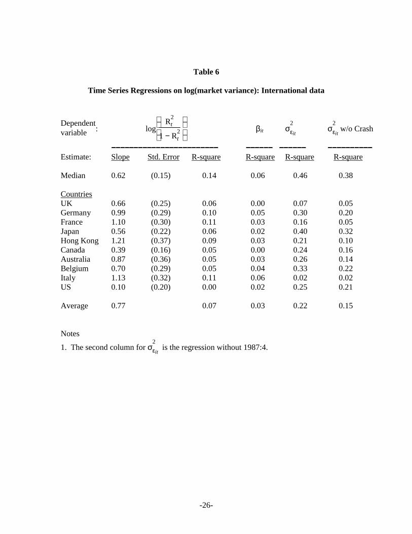
Table 6 confirms these results on a country-by-country basis. The R-squares of

the regressions of beta against market volatility are very small, but the R-squares of the

regressions of residual risk against market volatility average .15 even if we exclude the

Crash of 1987:4. This is actually double the average R-square of the relationship

between (transformed) country R-squares and market volatility.

The ability of the index model to capture international correlation patterns is not

as strong as in the domestic setting. As in Figure 4, Figure 8 plots the constrained R-

square in each quarter for each country against the realized R-square. The positive

association is obvious, but the fit is not as tight as in Figure 4.

-17-

Figure 9 shows that even with the greater variability in country returns, there may

be some value to using the index model to forecast cross-country correlations. The

median correlation does rise noticeably with the forecast of index variability derived

from an AR1 process.

Table 7 documents that the index model provides predictions that are only

marginally better than its competitors. We see in column 2 (Grand standard deviation)

that the variability of the covariance prediction from the index model is slightly less than

that of the current covariance estimator or the estimators based on actual market

volatility. The values for root mean square error or mean absolute error show again that

knowing market volatility would help in forecasting covariance structure. Here,

however, the advantage it would convey is not nearly as large. The forecast errors for the

predictions based on perfect foresight of market variance were only about one-fourth

those of the feasible forecasts in the domestic setting. Here, they are more like three-

fourths as large. The forecasts based on the index model are slightly better than the

alternative feasible models, but not to an extent that would make much difference in

practice.

4. Summary

This paper uses an index model to shed light on the variation through time of

asset correlation structure. Our model captures the empirical tendency for cross-sector

correlations tend to increase with the volatility of the market-wide, systematic factor.

We find that a large fraction of the time-variation in cross-industry correlation can

be attributed to variation in the volatility of the market index. Moreover, there is enough

-18-

predictability in index volatility to allow us to construct useful forecasts of covariance

matrices in coming periods. Minimum-variance portfolios constructed from covariance

matrices based on an index model and predicted market volatilities will perform

substantially better than ones that do not account for the impact of time-varying volatility

on correlation and covariance structure.

Our results for cross-country correlation structure are qualitatively the same as for

the domestic setting. However, there is considerably more country-specific risk than

industry-specific risk, implying that the proposed methodology to reduce the

dimensionality of the forecasting problem will be less successful in the international

setting.

-19-

References

Carol Alexander, (1992) “History Debunked”, Risk Magazine, vol. 5, no. 8.

F. Black, (1976), “Studies of Stock Market Volatility Changes,” Proceedings ofthe American Statistical Association, Business and Economic Statistics Section, 177-181.

T. Bollerslev , (1990), _________________________________.

T. Bollerslev , R. Chou, and K. Kroner, (1992), “ARCH Modeling in Finance: AReview of the Theory and Empirical Evidence,” Journal of Econometrics, 52, 5-59.

Z. Bodie A. Kane and A. J. Marcus, Investments, Irwin/McGraw-Hill, 1988,Fourth edition, 1998.

L.K.C. Chan, J. Karceski, and J. Lakonishok (1999), “On Portfolio Optimization:Forecasting Covariances and Choosingthe Risk Model,” Journal of Finance, 12, 937-974.

G. Chow, E. Jacquier, M. Kritzman and K. Lowry (1999), “Optimal Portfolios inGood Times and Bad,” Financial Analysts Journal, 55, No. 3.

M. Fridman, and L. Harris, (1998), “A Maximum Likelihood Approach for Non-Gaussian Stochastic Volatility Models,” Journal of Business and Economics Statistics,16, 3, 284-291.

Francois Longin, and Bruno Solnik, (1995), “Is the Correlation in InternationalEquity Returns Constant: 1960-1990?” Journal of International Money and Finance 14,3-26.

E. Jacquier, N. Polson, and P. Rossi, (1995), “Stochastic Volatility: Univariateand Multivariate Extensions,” Rodney L. White Center for Financial Research workingpaper 19-95, Wharton School.

Bruno Solnik, Cyril Boucrelle, and Yann Le Fur, (September/October 1996),“International Market Correlation and Volatility,” Financial Analysts Journal, 17-34.

D. Nelson, (1991), “Conditional Heteroskedasticity in Asset Pricing: A NewApproach,” Econometrica, 59, 347-370.

D. Nelson, (1992), “Getting the right variance with the wrong model,” Journal ofEconometrics, 52.

F.K. Reilly (1994), Investment Analysis and Portfolio Management, Dryden Press, 4th ed.

William F. Sharpe, (1963), “A Simplified Model of Portfolio Analysis,”Management Science, January.

-20-

______, G. J. Alexander , and J.V. Bailey, Investments, Prentice Hall, 1999, 6th ed.

S. Taylor (1976), Modelling Financial Time Series, New York: John Wiley &Sons.

-21-

Table 1: US Industry Portfolio Groups

Portfolio 2-Digit SIC Code Name 1 13,29 Petroleum2 60-69 Finance/Real Estate3 25, 30, 36, 37, 50, 55, 57 Consumer Durables4 10,12,14,24,26,28,33 Basic Industries5 1, 20, 21, 54 Food/Tobacco6 15-17, 32, 52 Construction7 34,35,38 Capital Goods8 40-42,44,45,47 Transportation9 46,48,49 Utilities10 22,23,31,51,53,56,59 Textiles/Trade11 72,73,75,80,82,89 Services12 27,58,70,78-79 Leisure

-22-

Table 2: Regressions of (transformed) ρρρρij against log(σσσσM)

For each of the 66 pairs of industries, we used daily data within the quarter to calculate

the correlation coefficient ρij. We then regressed the time series of ln(1 + ρij

1 − ρij)against

log(σM). The regressions are rank-ordered by slope coefficient. The slope, t-statistic forthat slope, and R-square for various percentile industry-pairs are reported in the table.(The first column reports the regression results for the median ρij of each quarter. Thismedian generally corresponds to different industry pairs each quarter, so the results formedian ρij differ from the fiftieth percentile regression, which is for a specific industrypair.

Median ρij Min 10% 25% 50% 75% 90% Max

Slope 1.49 1.08 1.22 1.41 1.51 1.56 1.62 1.78

t-statistic 22.1 10.4 11.6 12.8 16.5 17.7 18.6 20.0

R-square 0.78 0.43 0.49 0.54 0.66 0.69 0.71 0.74

-23-

Table 3: Time Series Regressions on log(market variance)

Dependentvariable : log

R

2t

1 − R2t

βit σ2

εit

−−−−−−−−−−−−−−−−−−−−−−−−−−−−−−−−−−−−−−−−−−−−−−−−−−−−−−−−−−−−−−−−−−−−−−−−−−−−−−−−−−−−−−−−−−−−−−−− −−−−−−−−−−−−−−−−−−−−−−−− −−−−−−−−−−−−−−−−−−−−−−−−Estimate: Slope Std. Error R-square R-square R-square

Mediana: 0.82 NA 0.75 0.02 0.08

Industries:1 0.87 (0.10) 0.35 0.03 0.122 0.81 (0.07) 0.48 0.05 0.033 0.85 (0.04) 0.73 0.00 0.084 0.81 (0.06) 0.61 0.04 0.065 0.90 (0.05) 0.65 0.07 0.006 0.93 (0.06) 0.65 0.01 0.007 0.86 (0.05) 0.69 0.01 0.048 0.87 (0.06) 0.62 0.03 0.029 0.56 (0.07) 0.32 0.05 0.1610 0.81 (0.05) 0.67 0.01 0.0411 0.83 (0.08) 0.46 0.01 0.0412 0.92 (0.05) 0.68 0.00 0.02

Average: 0.79 0.58 0.03 0.05

Notes:

a. This is the regression of the median value for log[R2/(1−R2)] in each quarter againstmarket volatility. The identity of the median industry pair will differ across quarters.

-24-

Table 4: Properties of Covariance Estimators

EstimatorGrand Mean

GrandStandard

Deviation

GrandMeanError

Root MeanSquare Error

MeanAbsolute

Error

Current covariance 0.0107 0.0169 -0.0001 0.0223 0.0086Full-sample covariance 0.0113 0.0025 0.0007 0.0167 0.0080Index model(t-1) 0.0105 0.0161 -0.0001 0.0219 0.0087Index model(AR1) 0.0087 0.0035 -0.0200 0.0168 0.0066Index model(t) 0.0106 0.0161 0.0000 0.0040 0.0019

Notes:

1. 141 quarters, 66 covariances each quarter

2. Current covariance: for each industry pair, the forecast of next period’s covariance isthis period’s covariance.

Full sample covariance is the estimate obtained by pooling all daily returns into oneperiod and calculating the single full-sample-period covariance matrix.

Index model estimate is the prediction from the constrained index model where onlymarket variance is allowed to vary over time. Index model(t) denotes use of the next-period market variance to calculate next-period covariance, Index model(t-1) denotesthe use of current market variance, and Index model(AR1) denotes the use of theprediction of the future market variance from the AR1 model.

-25-

Table 5

Regressions of (transformed) ρρρρij against log(σσσσM): International data

For each of the 45 pairs of countries, we used daily data within the quarter to calculate

the correlation coefficient ρij. We then regressed the time series of ln(1 + ρij

1 − ρij)against

log(σM). The regressions are rank-ordered by slope coefficient. The slope, t-statistic forthat slope, and R-square for various percentile country-pairs are reported in the table.(The first column reports the regression results for the median ρij of each quarter. Thismedian generally corresponds to different country pairs each quarter, so the results formedian ρij differ from the fiftieth percentile regression, which is for a specific countrypair.

Median ρij Min 10% 25% 50% 75% 90% Max

Slope 0.44 0.17 0.30 0.38 0.43 0.53 0.70 0.89t-stat 5.55 1.64 2.50 3.18 3.84 4.53 4.88 5.53Rsquare 0.23 0.03 0.06 0.09 0.12 0.16 0.19 0.23

-26-

Table 6

Time Series Regressions on log(market variance): International data

Dependentvariable : log

R

2t

1 − R2t

βit σ2

εit σ

2

εit w/o Crash

−−−−−−−−−−−−−−−−−−−−−−−−−−−−−−−−−−−−−−−−−−−−−−−−−−−−−−−−−−−−−−−−−−−−−−−−−−−−−−−−−−−−−−−−−−−−−−−− −−−−−−−−−−−−−−−−−−−−−−−− −−−−−−−−−−−−−−−−−−−−−−−− −−−−−−−−−−−−−−−−−−−−−−−−−−−−−−−−−−−−−−−−Estimate: Slope Std. Error R-square R-square R-square R-square

Median 0.62 (0.15) 0.14 0.06 0.46 0.38

Countries UK 0.66 (0.25) 0.06 0.00 0.07 0.05Germany 0.99 (0.29) 0.10 0.05 0.30 0.20France 1.10 (0.30) 0.11 0.03 0.16 0.05Japan 0.56 (0.22) 0.06 0.02 0.40 0.32Hong Kong 1.21 (0.37) 0.09 0.03 0.21 0.10Canada 0.39 (0.16) 0.05 0.00 0.24 0.16Australia 0.87 (0.36) 0.05 0.03 0.26 0.14Belgium 0.70 (0.29) 0.05 0.04 0.33 0.22Italy 1.13 (0.32) 0.11 0.06 0.02 0.02US 0.10 (0.20) 0.00 0.02 0.25 0.21

Average 0.77 0.07 0.03 0.22 0.15

Notes

1. The second column for σ2

εit is the regression without 1987:4.

-27-

Table 7

Properties of Covariance Estimators: International Data

EstimatorGrand Mean

GrandStandard

Deviation

GrandMeanError

Root meansquare error

Meanabsolute

errorCurrent covariance 0.0063 0.0159 -0.0001 0.0203 0.0078Full-sample covariance 0.0065 0.0025 0.0002 0.0157 0.007Index model(t-1) 0.0065 0.0058 0.0001 0.0158 0.0068Index model(AR1) 0.006 0.0031 -0.0003 0.0155 0.0065Index model(t) 0.0065 0.0058 0.0001 0.0122 0.0057

Notes:

1. 105 quarters, 45 covariances each quarter

2. 2. Current covariance: for each country pair, the forecast of next period’s covarianceis this period’s covariance.

Full sample covariance is the estimate obtained by pooling all daily returns into oneperiod and calculating the single full-sample-period covariance matrix.

Index model estimate is the prediction from the constrained index model where onlymarket variance is allowed to vary over time. Index model(t) denotes use of the next-period market variance to calculate next-period covariance, Index model(t-1) denotesthe use of current market variance, and Index model(AR1) denotes the use of theprediction of the future market variance from the AR1 model.