Computer Architecture Guidance Keio University AMANO, Hideharu hunga@am . ics . keio . ac . jp.

Proceedings of the Asia Pacific Industrial Engineering & Management Systems Conference 2017
1
Asset Allocation Model with Tail Risk Parity
Hirotaka Kato† Graduate School of Science and Technology
Keio University, Yokohama, Japan
Tel: (+81) 45-566-1454, Email: [email protected]
Norio Hibiki
Faculty of Science and Technology
Keio University, Yokohama, Japan
Tel: (+81) 45-466-1635, Email: [email protected]
Abstract. Asset allocation strategy is important to manage assets effectively. In recent years, risk parity strategy
attracts attention in place of traditional mean-variance approach. Risk parity portfolio is one of the risk-based
portfolios, and it equalizes risk contributions across all assets included in the portfolio. Specifically, the equally-
weighted risk contribution is calculated by decomposing the standard deviation of the portfolio’s return. In addition,
some studies propose the tail risk parity strategy which equalizes the risk contribution of downside risk measure
(Alankar et al., 2012, Boudt et al., 2013), and use conditional value-at-risk (CVaR) as a risk measure. In this paper,
we first compare tail risk parity strategies with CVaRs estimated by three kinds of estimation methods (Delta-normal
method, historical-simulation method, and Monte Carlo method), and examine the characteristics of the risk parity
portfolios. We also implement the backtest for eighteen years using the historical data of Nikkei 225, Citi JPGBI
(Japan government bond index), S&P500, and Citi USGBI. We find the estimated expect return and distribution affect
optimal investment ratios and portfolio’s performance, but mutual dependence between assets does not affect them.
Keywords: finance, asset allocation, risk parity, risk budget, down side risk
1. Introduction
Asset allocation strategy is important to manage assets
effectively. The standard asset allocation model is the mean-
variance model. This model uses expected returns, standard
deviations and correlations of assets, optimal portfolio is
uniquely determined to express investor’s risk preference by
risk aversion. However, mean-variance optimal portfolio’s
weights are extremely sensitive to the change in parameters,
especially expected returns. In recent years, many researchers
have shown interests in the approach of constructing portfolio,
using risk due to the difficulty of estimating expected returns.
Many studies attribute the better performance of these risk-
based asset allocation approaches. In particular, risk parity
portfolio attracts attention among practitioners and researchers.
The approach equalizes risk contributions which is the
decomposition of the total risk to each individual asset. The
total risk can be the standard deviation of the portfolio return
across all assets in general. In contrast, some studies propose
the tail risk parity portfolio which equalizes risk contributions
of downside risk measure (Alankar et al., 2012, Boudt et al.,
2013). Few studies examine the effect of choosing risk
1 CVaR is referred to as tail VaR, expected shortfall, conditional tail expectation.
measure and how to estimate downside risks. It is important to
investigate the difference between general risk parity portfolio
and tail risk parity portfolio.
In this paper, we construct tail risk parity portfolio using
conditional value-at-risk(CVaR)1 as downside risk. At first,
we compare tail risk parity strategies with CVaRs estimated by
three kinds of estimation methods (Delta-normal method,
historical-simulation method, and Monte Carlo method), and
examine the characteristics of the tail risk parity portfolios.
Second, we implement the backtest for eighteen years using
the historical data of Nikkei 225, Citi JPGBI (Japan
government bond index), S&P500, and Citi USGBI, and we
discuss the advantage of tail risk parity portfolio.
We find that the tail risk parity portfolio outperforms the
usual risk parity portfolio. We decompose the difference of
performance between them into three factors; 1. expected
return, 2. distribution and 3. mutual dependence. The result
shows that outperformance attributes to the expected return.
Examining the distributions other than the normal distribution,
the absolute return decreases, but the efficiency measure
increases. The mutual dependence does not affect the
difference of performance.
Kato and Hibiki
2
2. Risk Parity Portfolio
We define each asset’s risk contribution. The most
commonly used definition is based on Euler’s homogeneous
function theorem. It is defined as follows,
𝑅𝐶𝑖 = 𝑤𝑖
𝜕𝑅(𝑤)
𝜕𝑤𝑖
=𝜕𝑅(𝑤)
𝜕𝑤𝑖/𝑤𝑖
(1)
where 𝑅(𝑤) is portfolio risk, and 𝑤𝑖 is portfolio weight to
asset i. Risk contribution is calculated as the sensitivity of
the change in portfolio risk to the change in each weight.
We satisfy the following equation.
𝑅(𝑤) = ∑ 𝑅𝐶𝑖
𝑛
𝑖=1
(2)
Equation (2) shows that the total portfolio risk equals the
sum of each asset risk contribution by Euler’s homogeneous
function theorem.
Risk parity strategy utilizes standard deviation of
portfolio return and equalizes its risk contribution across all
assets. Using the method, the portfolio risk can be equally
diversified to each asset.
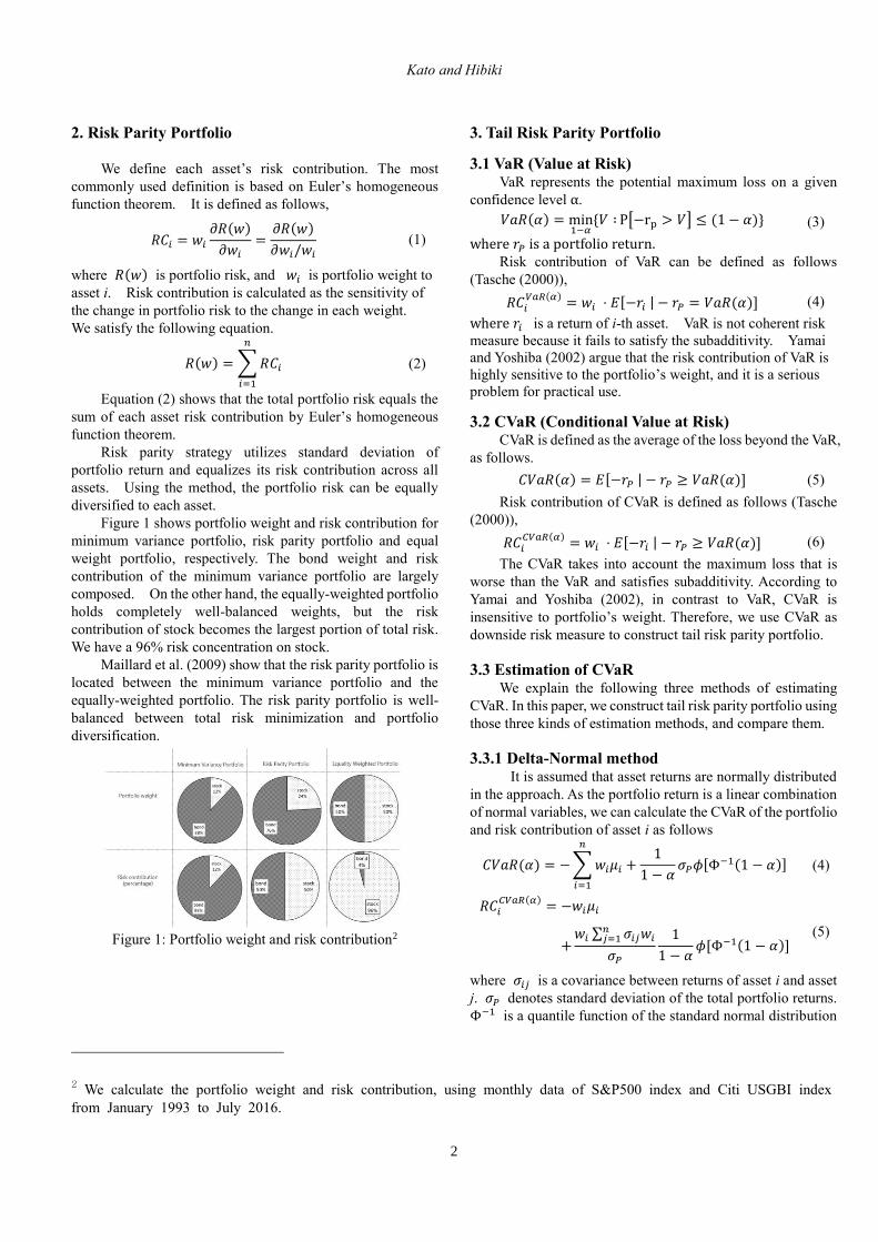
Figure 1 shows portfolio weight and risk contribution for
minimum variance portfolio, risk parity portfolio and equal
weight portfolio, respectively. The bond weight and risk
contribution of the minimum variance portfolio are largely
composed. On the other hand, the equally-weighted portfolio
holds completely well-balanced weights, but the risk
contribution of stock becomes the largest portion of total risk.
We have a 96% risk concentration on stock.
Maillard et al. (2009) show that the risk parity portfolio is
located between the minimum variance portfolio and the
equally-weighted portfolio. The risk parity portfolio is well-
balanced between total risk minimization and portfolio
diversification.
Figure 1: Portfolio weight and risk contribution2
2 We calculate the portfolio weight and risk contribution, using monthly data of S&P500 index and Citi USGBI index
from January 1993 to July 2016.
3. Tail Risk Parity Portfolio
3.1 VaR (Value at Risk) VaR represents the potential maximum loss on a given
confidence level α.
𝑉𝑎𝑅(𝛼) = min1−𝛼
{𝑉 ∶ P[−rp > 𝑉] ≤ (1 − 𝛼)} (3)
where 𝑟𝑃 is a portfolio return. Risk contribution of VaR can be defined as follows
(Tasche (2000)),
𝑅𝐶𝑖𝑉𝑎𝑅(𝛼)
= 𝑤𝑖 ⋅ 𝐸[−𝑟𝑖 | − 𝑟𝑃 = 𝑉𝑎𝑅(𝛼)] (4)
where 𝑟𝑖 is a return of i-th asset. VaR is not coherent risk
measure because it fails to satisfy the subadditivity. Yamai
and Yoshiba (2002) argue that the risk contribution of VaR is
highly sensitive to the portfolio’s weight, and it is a serious
problem for practical use.
3.2 CVaR (Conditional Value at Risk) CVaR is defined as the average of the loss beyond the VaR,
as follows.
𝐶𝑉𝑎𝑅(𝛼) = 𝐸[−𝑟𝑃 | − 𝑟𝑃 ≥ 𝑉𝑎𝑅(𝛼)] (5)
Risk contribution of CVaR is defined as follows (Tasche
(2000)),
𝑅𝐶𝑖𝐶𝑉𝑎𝑅(𝛼)
= 𝑤𝑖 ⋅ 𝐸[−𝑟𝑖 | − 𝑟𝑃 ≥ 𝑉𝑎𝑅(𝛼)] (6)
The CVaR takes into account the maximum loss that is
worse than the VaR and satisfies subadditivity. According to
Yamai and Yoshiba (2002), in contrast to VaR, CVaR is
insensitive to portfolio’s weight. Therefore, we use CVaR as
downside risk measure to construct tail risk parity portfolio.
3.3 Estimation of CVaR We explain the following three methods of estimating
CVaR. In this paper, we construct tail risk parity portfolio using
those three kinds of estimation methods, and compare them.
3.3.1 Delta-Normal method It is assumed that asset returns are normally distributed
in the approach. As the portfolio return is a linear combination
of normal variables, we can calculate the CVaR of the portfolio
and risk contribution of asset i as follows
𝐶𝑉𝑎𝑅(𝛼) = − ∑ 𝑤𝑖𝜇𝑖
𝑛
𝑖=1
+1
1 − 𝛼𝜎𝑃𝜙[Φ−1(1 − 𝛼)] (4)
𝑅𝐶𝑖𝐶𝑉𝑎𝑅(𝛼)
= −𝑤𝑖𝜇𝑖
+𝑤𝑖 ∑ 𝜎𝑖𝑗𝑤𝑖
𝑛𝑗=1
𝜎𝑃
1
1 − 𝛼𝜙[Φ−1(1 − 𝛼)]
(5)
where 𝜎𝑖𝑗 is a covariance between returns of asset i and asset
j. 𝜎𝑃 denotes standard deviation of the total portfolio returns.
Φ−1 is a quantile function of the standard normal distribution

Kato and Hibiki
3
and 𝜙 is a standard normal density function. This method is
very practical and easy to use. However, many empirical
studies show that returns of financial assets do not follow the
normal distribution and the assumption of normally distributed
financial returns underestimates VaR and CVaR.
3.3.2 Historical-Simulation method This method is a non-parametric approach to estimate
CVaR based on historical data. The CVaR (and VaR) can be
calculated using the percentile of the empirical distribution
corresponding to a given confidence level. This method can be
applied to the non-normal distributions with heavy tails.
However, the calculation is sensitive to the abnormal
observation. This feature is inconvenient for constructing tail
risk parity portfolio. Thus, we generate random numbers for
the distribution which are obtained by kernel smoothing from
the observed data. Suppose {𝑥1, 𝑥2, … , 𝑥𝑛} denotes data
observations for each asset. Kernel-smoothed cumulative
distribution function (cdf) is
𝑓(𝑥) =1
𝑛ℎ∑ 𝐾 (
𝑥 − 𝑥𝑖
ℎ)
𝑛
𝑖=1
, (6)
where 𝐾(⋅) is a kernel function. It is the empirical distribution.
Parameter h is the bandwidth or smoothing parameter. It
controls the smoothness of the estimated cdf. We determine the
bandwidth using the method of Matt and Jones (1994). We
employ the Gaussian kernel function which is a commonly
used.
𝐾(𝑢) = (2𝜋)−1/2𝑒−𝑢2/2 (7)
Figure 2: Kernel Smoothed functions
3.3.3 Monte Carlo method The probability distribution and the dynamics of asset
3 The DFO method is the non-linear optimization method where the problems are solved without the derivative of the objective
function. The type of the problem goes well with the DFO method. We used Numerical Optimizer/DFO added on the
mathematical programming software package called Numerical Optimizer (ver. 18.1.0) developed by NTT DATA Mathematical
System, Inc. 4 The weights of inverse volatility portfolio are calculated as 𝑤𝑖 = 𝜎𝑖/ ∑ 𝜎𝑗
𝑁𝑗=1 . This portfolio is equal to the risk parity
portfolio when the correlations between assets are zero. Even if assets are correlated, it is expected that the portfolio takes a close
value to tail risk parity or risk parity portfolio.
prices are simulated by generating random samples. It allows
for any distribution (even non-normal distribution) and non-
linear dependence. We generate random numbers which
follows GH (Generalized Hyperbolic) distribution, and mutual
dependence between assets represented by t-Copula. GH
distribution is flexible enough to express fat tail and
asymmetry. Copula describes dependence structure between
each asset and can captures the tail of marginal distributions,
unlike a linear correlation. We estimate GH distribution and t-
Copula parameters by maximum likelihood method.
3.4 Formulation of asset allocation model with tail risk parity
We build tail risk parity portfolio which equalize all
asset’s risk contribution of CVaR. The model can be
formulated as follows,
1 Sets
𝐹 ∶ set of foreign assets
2 Parameters
𝑁 ∶ number of assets
𝑑 ∶ risk-free interest rate of Japanese yen
𝑓 ∶ risk-free interest rate of U.S. dollar
𝛼 ∶ confidence level of CVaR
3 Decision variables
𝑤𝑖 ∶ portfolio weight of asset 𝑖
Minimize ∑ (𝑅𝐶𝑖
𝐶𝑉𝑎𝑅(𝛼)
𝐶𝑉𝑎𝑅𝑃(𝛼)−
1
𝑁)
2𝑁
𝑖=1
(8) subject to ∑ 𝑤𝑖 + ∑(𝑓 − 𝑑)𝑤𝑗 = 1
𝑗∈𝐹
𝑁
𝑖=1
𝑤𝑖 ≥ 0, 𝑖 ∈ {1,2, … , 𝑁}
We solve the problem under the perfect hedging strategy
for foreign assets. The hedging cost is the difference between
U.S. and Japanese interest rate.
Problem (8) is difficult to solve using a commonly used
mathematical programming tool because the objective
function is non-convex, and RC and CVaR cannot be also
expressed with the explicit function of the decision variables.
Therefore, we used DFO3 (Derivative Free Optimizer) method
to solve the problem. However, the problem is dependent on
an initial value, and then we set inverse volatility portfolio4 as
the initial portfolio weight.

Kato and Hibiki
4
Table 1: Comparisons5
Case 1 2 3 4 5 6
Risk measure
(estimation method of
CVaR)
standard
deviation
CVaR
(Delta-Normal
method)
CVaR
(Historical-
Simulation
method)
CVaR
(Monte Carlo
method)
CVaR
(Monte Carlo
method)
CVaR
(Historical-
Simulation
method)
Estimation of expected
return No Yes No (μi = 0) No (μi = 0) No (μi = 0) Yes
Probability distribution normal normal historical GH normal historical
Mutual dependence
linear
correlation
(=Gaussian
copula)
linear
correlation
(=Gaussian
copula)
Gaussian
copula
Gaussian
copula t-copula t-copula
4. Basic Analysis
We conduct the analysis for two-asset tail risk parity
portfolio which consists of domestic stock and bond. We
employ monthly data from January 1993 to July 2016 for
Nikkei 225 stock and Citi JPGBI(Japan Government Bond
Index). Summary statistics are shown in Table 2.
We set four kinds of the confidence level; 0.80, 0.85, 0.90,
0.95. The number of simulation paths is 20,000. We compare
six cases in Table 1 in order to examine the difference between
risk parity and tail risk parity portfolio.
Table 2: Statistics of return on an annual basis
stock bond
Mean 2.04% 3.24%
Standard deviation 20.20% 3.15%
Skewness -0.323 -0.363
Exceed kurtosis 0.517 5.154
4.1 Expected return We can construct risk parity portfolio without estimating
expected returns. Some researchers say that this is one reason
why risk parity portfolio has better performance than other
portfolios. However, we need to estimate expected return to
construct tail risk parity portfolio. Several studies have proved
that it is difficult to estimate expected return. We pay attention
to the fact that estimation errors of the expected return may
affect the optimal portfolio. In our paper, we calculate
average return in all period.
The difference of cases 1 and 2 in Table 1 is dependent on
the expected return of asset because the CVaR is calculated in
proportion to the standard deviation. Therefore, we compare
the two cases, and examine the effect on the expected return
for the tail risk parity portfolio.
5 μi = 0 indicates asset return is normalized so that each mean return can be zero.
Table 3: Comparison of the portfolio weights for the different
expected returns
α = 0.80 Case 1 Case 2
Stock 13.53% 12.19%
Bond 86.47% 87.81%
Table 3 shows the weights of each portfolio. Expected
returns are 2.04% for stock and 3.24% for bond. The stock
weight of tail risk parity portfolio is less than that of risk parity
portfolio. The reason is that the asset with relatively higher
expected return is allocated more in the tail risk parity portfolio.
In addition, we find the difference tends to decrease as the
confidence level becomes higher.
4.2 Distribution We examine the effect on the distribution to compare case
1 and case 3(Historical-Simulation method) or case 4(Monte
Carlo method) in Table 1.
Table 4: Comparison for the different distribution
α = 0.80 Case 1 Case 3 Case 4
Stock 13.53% 12.59% 12.49%
Bond 86.47% 87.41% 87.51%
α = 0.95 Case 1 Case 3 Case 4
Stock 13.53% 14.37% 13.75%
Bond 86.47% 85.63% 86.25%
Table 4 shows the weights of each portfolio in 0.80 and
0.95 confidence levels, respectively. Bond has lower skewness
and higher kurtosis than stock.
According to cases 3 and 4, the weight of bond in tail risk
parity portfolio decreases as the confidence level becomes
higher. Examining the relationship between confidence level
and distribution is our future task.
4.3 Mutual dependence Describing the mutual dependence, non-linear correlation
can be involved in the tail risk parity portfolio whereas
Kato and Hibiki
5
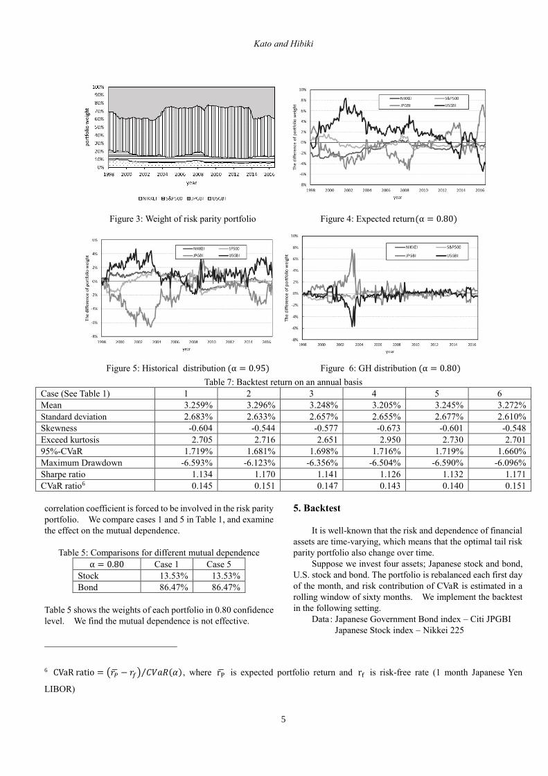
Figure 3: Weight of risk parity portfolio Figure 4: Expected return(α = 0.80)
Figure 5: Historical distribution (α = 0.95) Figure 6: GH distribution (α = 0.80)
Table 7: Backtest return on an annual basis
Case (See Table 1) 1 2 3 4 5 6
Mean 3.259% 3.296% 3.248% 3.205% 3.245% 3.272%
Standard deviation 2.683% 2.633% 2.657% 2.655% 2.677% 2.610%
Skewness -0.604 -0.544 -0.577 -0.673 -0.601 -0.548
Exceed kurtosis 2.705 2.716 2.651 2.950 2.730 2.701
95%-CVaR 1.719% 1.681% 1.698% 1.716% 1.719% 1.660%
Maximum Drawdown -6.593% -6.123% -6.356% -6.504% -6.590% -6.096%
Sharpe ratio 1.134 1.170 1.141 1.126 1.132 1.171
CVaR ratio6 0.145 0.151 0.147 0.143 0.140 0.151
correlation coefficient is forced to be involved in the risk parity
portfolio. We compare cases 1 and 5 in Table 1, and examine
the effect on the mutual dependence.
Table 5: Comparisons for different mutual dependence
α = 0.80 Case 1 Case 5
Stock 13.53% 13.53%
Bond 86.47% 86.47%
Table 5 shows the weights of each portfolio in 0.80 confidence
level. We find the mutual dependence is not effective.
6 CVaR ratio = (𝑟�̅� − 𝑟𝑓) 𝐶𝑉𝑎𝑅(𝛼)⁄ , where rP̅ is expected portfolio return and rf is risk-free rate (1 month Japanese Yen
LIBOR)
5. Backtest
It is well-known that the risk and dependence of financial
assets are time-varying, which means that the optimal tail risk
parity portfolio also change over time.
Suppose we invest four assets; Japanese stock and bond,
U.S. stock and bond. The portfolio is rebalanced each first day
of the month, and risk contribution of CVaR is estimated in a
rolling window of sixty months. We implement the backtest
in the following setting.
Data : Japanese Government Bond index – Citi JPGBI
Japanese Stock index – Nikkei 225

Kato and Hibiki
6
U.S. Government Bond index – Citi USGBI
U.S. Stock index–S&P500
Period: January 1993 – July 2016, monthly data
Currency hedging strategy: perfect hedging on a yen basis
Hedge cost: difference between U.S. and Japanese
interest rate (one month LIBOR)
Number of simulation paths: 20,000 paths
We examine the results of the backtest as well as the basic
analysis. We show the results for the confidence level where
the difference of the portfolio weights between tail risk parity
portfolio and risk parity portfolio is the largest (Figure 3 shows
risk parity portfolio’s weight).
5.1 Expected return Figure 4 shows the difference of portfolio weights (tail
risk parity portfolio minus risk parity portfolio) between
cases 1 and 2 as in the basis analysis. The portfolio weight of
U.S. bond has increased relatively toward 2002 due to the rise
in expected return of U.S. bond.
As shown in Table 7, the tail risk parity portfolio
outperforms the risk parity portfolio due to the effect of
expected return.
5.2 Distribution Similarly, Figures 5 and 6 show the difference of portfolio
weights for different distributions, respectively.
Figure 5 shows the difference calculated using the
historical simulation method between cases 1 and 3. The
weight of Japanese bond has decreased relatively due to the
decrease in skewness of the return. Figure 6 shows the
difference calculated using Monte Carlo method under the GH
distribution between cases 1 and 4. In contrast, the weight of
Japanese bond has increased relatively due to the increase in
kurtosis in 2003.
Table 7 indicates the absolute return goes down but the
efficiency index goes up in the historical simulation.
However, various statistics and efficiency index go down in
Monte Carlo method under the GH distribution, compared with
risk parity portfolio. The reason is that overinvesting Japanese
Government Bonds has greatly influenced the 2003 VaR
shock7 in Japan.
5.3 Mutual dependence The differences in the portfolio weights between cases 1
and 5 remain within the range of 1% in all period, and then we
could not find the effect due to the non-linear dependence.
6. Conclusion
We compare the tail risk parity strategy using the
following three estimation methods of CVaR; Delta-normal
method, Historical-simulation method and Monte Carlo
7The 10 year JGB yield triples from 0.5% in June 2003 to 1.6% in September 2003.
method. We also clarify the difference of risk parity portfolio
and tail risk parity portfolio due to the following three factors;
expected return, distribution and mutual dependence.
In the basic analysis, we find we invest in the assets with
higher expected return and skewness in the tail risk parity
portfolio. This result is reasonable to the expected utility theory.
On the other hand, we tend to invest in the assets with higher
kurtosis at low confidence level. This result is the opposite to
the expected utility theory.
We also implement the backtest using historical data of
Japanese stock and bond, U.S. stock and bond. The
portfolio return of tail risk parity with historical-simulation
method, has declined, but the efficiency index is rising. On
the other hand, Monte Carlo method assuming GH
distribution, various statistics and efficiency index
deteriorated compared with usual risk parity portfolio. In this
paper, we could not find the effect of non-linear dependence.
In the future research, we need to determine how to set
parameters and how to decide the distribution to use the tail
risk parity strategy in practice. We also need to compare with
different risk parity strategies using downside risk measures.
REFERENCES Asness, C.S., A.Frazzini, and L.H. Pedersen (2012). Leverage
aversion and risk parity. Financial Analysts Journal 68(1),
47-59.
Alankar, A., M. DePalma and M. Scholes (2013). An
introduction to tail risk parity: Balancing risk to achieve
downside protection. AllianceBernstein. white paper.
Available at: https://www.abglobal.com/abcom/segment_
homepages/defined_benefit/3_emea/content/pdf/introducti
on-to-tail-risk-parity.pdf
Boudt, K., P. Carl and B.G. Peterson (2013). Asset allocation
with conditional value-at-risk budgets. The Journal of Risk,
15(3), 39-68.
Butler, J. S., and B. Schachter (1997). Estimating value-at-risk
with a precision measure by combining kernel estimation
with historical simulation. Review of Derivatives Research,
1, 371-390.
Maillard, S., T. Roncalli and J. Teïletche (2010). The properties
of equally weighted risk contribution portfolios. The
Journal of Portfolio Management, 36(4), 60-70.
Tasche, D. (1999). Risk contributions and performance
measurement. Report of the Lehrstuhl für mathematische
Statistik, TU München.
Yamai, Y., and T. Yoshiba (2002). Comparative analyses of
expected shortfall and value-at-risk: their estimation error,
decomposition, and optimization. Monetary and economic
studies, 20(1), 87-121.
Wand, M. P. and M.C. Jones (1994). Kernel smoothing. Crc
Press.