Assessors' Handbook Section 582, The Explanation … present worth factor for the total life of the...

ASSESSORS' HANDBOOK SECTION 582

THE EXPLANATION OF THE DERIVATION OF EQUIPMENT PERCENT GOOD FACTORS

FEBRUARY 1981

REPRINTED JANUARY 2015

CALIFORNIA STATE BOARD OF EQUALIZATION SEN. GEORGE RUNNER (RET.), LANCASTER FIRST DISTRICT

FIONA MA, CPA, SAN FRANCISCO SECOND DISTRICT JEROME E. HORTON, LOS ANGELES COUNTY THIRD DISTRICT DIANE L. HARKEY, ORANGE COUNTY FOURTH DISTRICT BETTY T. YEE, SACRAMENTO STATE CONTROLLER

__________________

CYNTHIA BRIDGES, EXECUTIVE DIRECTOR

AH 582 i February 1981

FOREWORD

Assessors’ Handbook Section 581A was written to serve as a permanent supplement toAssessors’ Handbook Section 581, Equipment Index Factors and Inventory Ratios, which isreissued annually. The sole intent of Assessors’ Handbook Section 581A is to provide a technicalexplanation of the mathematical origin of the percent good factors in Assessors’ HandbookSection 581 and to elucidate the usefulness and limitations of those factors.

Verne Walton, ChiefAssessment Standards DivisionDepartment of Property TaxesJanuary 1981

AH 582 ii February 1981

TABLE OF CONTENTS

CHAPTER 1: INTRODUCTION............................................................................................1

BASIS OF PERCENT GOOD ............................................................................................................1

CHAPTER 2: MORTALITY STUDIES.................................................................................3

AVERAGE SERVICE LIFE...............................................................................................................4PROBABLE TOTAL LIFE ................................................................................................................4REMAINING LIFE EXPECTANCY ....................................................................................................4SURVIVOR CURVES......................................................................................................................4RETIREMENT FREQUENCY CURVES...............................................................................................4THE MODAL YEAR.......................................................................................................................4

CHAPTER 3: THE ORGANIZATION OF THE IOWA STATE TABLES ..........................5

“R,” “ S,” AND “L” CURVES ........................................................................................................5VARIATIONS DUE TO MODAL YEAR RETIREMENT FREQUENCY .....................................................6THE SCOPE OF THE IOWA CURVES ................................................................................................8

CHAPTER 4: COMPUTING PERCENT GOOD..................................................................9

INCOME ADJUSTMENT FACTORS................................................................................................. 10THE GROUP METHOD................................................................................................................. 11THE GROUP FORMULA ............................................................................................................... 13

CHAPTER 5: THE EFFECT OF THE FOUR VARIABLES.............................................. 16

THE EFFECT OF THE YIELD RATE................................................................................................ 16THE EFFECT OF THE METHOD OF COMPUTATION ......................................................................... 18THE EFFECT OF THE INCOME ADJUSTMENT FACTOR.................................................................... 20THE EFFECT OF THE SURVIVOR CURVE....................................................................................... 21THE USE OF THE PERCENT GOOD FACTORS................................................................................. 21

AH 582 1 February 1981

CHAPTER 1: INTRODUCTION

Normal percent good tables have long been published in Assessors’ Handbook Section 581,Equipment Index Factors and Inventory Ratios. The intent of this report is to tell of theirderivation, their usefulness, and their limitations. Normal percent good factors help to provideone estimate of value, namely RCLND, which means replacement or reproduction cost new lessnormal depreciation. RCLND is not the answer to all property appraisals that employ the costapproach to value, but it is a significant aid in the mass appraisal of industrial machinery andequipment. Therefore, it is appropriate that appraisers who regularly compute RCLND, whetherby election or by policy, should understand the origin of the percent good factors they are using.

BASIS OF PERCENT GOOD

The value of a property is said to be equal to the present worth of its anticipated future netbenefits. Also, it is generally agreed that industrial property is owned primarily for its future netincome. It follows, then, that the value of an industrial property is equal to the present worth ofits future net income. The major problem with using this rationale in appraising industrialproperty is the almost impossible task of estimating net income accurately.

We can, however, use this idea in preparing percent good tables and avoid the critical problem ofestimating net income. If the only difference between an existing property and a similar newproperty is age or remaining life expectancy, a relationship between the two properties can becomputed using present worth factors. A present worth factor for the total life of the property isproportionate to the value of the new property, and the present worth factor for the remaining lifeis proportionate to the value of the existing property. By dividing the present worth of one perannum for the remaining life expectancy of a property by the present worth of one per annum forthe total life expectancy, the percent good can be calculated.

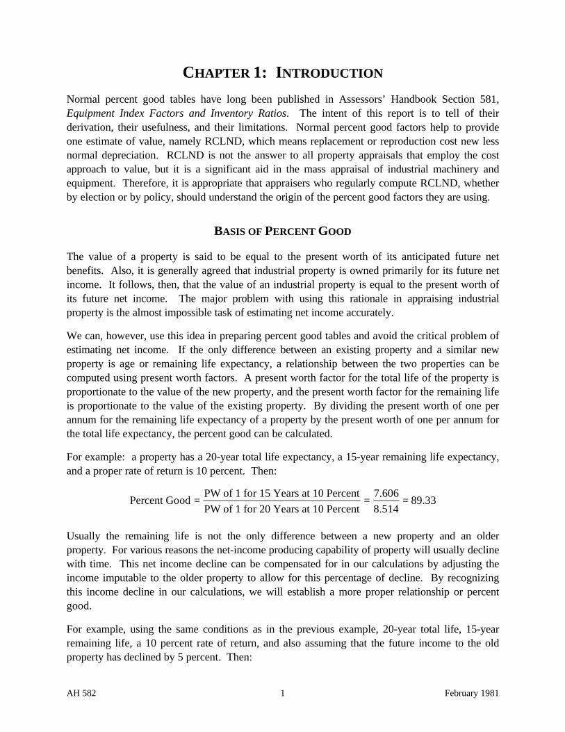
For example: a property has a 20-year total life expectancy, a 15-year remaining life expectancy,and a proper rate of return is 10 percent. Then:

PW of 1 for 15 Years at 10 Percent 7.606Percent Good = = = 89.33

PW of 1 for 20 Years at 10 Percent 8.514

Usually the remaining life is not the only difference between a new property and an olderproperty. For various reasons the net-income producing capability of property will usually declinewith time. This net income decline can be compensated for in our calculations by adjusting theincome imputable to the older property to allow for this percentage of decline. By recognizingthis income decline in our calculations, we will establish a more proper relationship or percentgood.

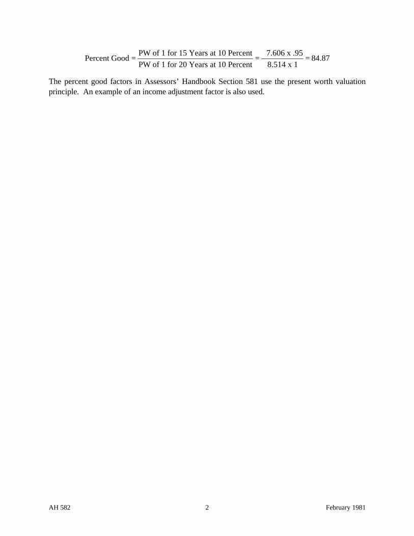
For example, using the same conditions as in the previous example, 20-year total life, 15-yearremaining life, a 10 percent rate of return, and also assuming that the future income to the oldproperty has declined by 5 percent. Then:


PW of 1 for 15 Years at 10 Percent 7.606 x .95Percent Good = = = 84.87

PW of 1 for 20 Years at 10 Percent 8.514 x 1

The percent good factors in Assessors’ Handbook Section 581 use the present worth valuationprinciple. An example of an income adjustment factor is also used.


CHAPTER 2: MORTALITY STUDIES

One of the necessary ingredients in computing these percent good factors is the relationshipbetween total life expectancy and probable remaining life expectancy of property items at allstages of their life. It may seem that if an item has a 20-year life expectancy when new that after20 years its life expectancy would be zero. This is not the case; any forecast of future events issubject to change with time. A new property is usually faced with many uncertainties. As timepasses and the property survives the test of time, the forecast of its total life expectancy willincrease.

Mortality studies are statistical studies based upon a sample group of a population. They state thepercentage of things which live at any given age and their life expectancy at any age. A group ofthings is identified, and a record of the life term of each one is made. The average life term orprobable life expectancy when new is computed by summing the life terms of all items in thegroup and dividing by the total number in the group. The probable total life expectancy ofsurvivors of the group is similarly computed by summing their total life expectancies and dividingby the number of survivors at that age.

We are all familiar with the actuarial tables compiled by insurance companies and used to predictthe life expectancy of humans at all ages. Similar studies have been conducted with various typesof industrial machinery and equipment by the engineering department of Iowa State University. Apart of the very useful data published as a result of this research is in the form of several series ofgraphs and tables which reflect the results of their studies.

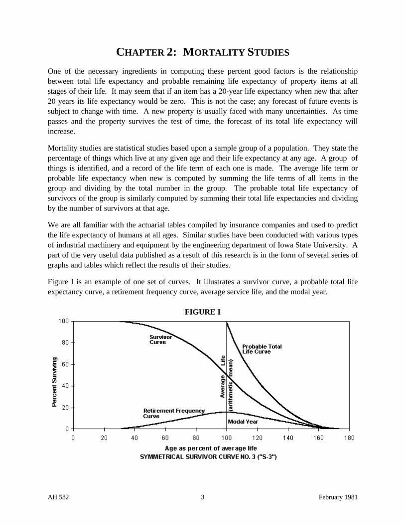
Figure I is an example of one set of curves. It illustrates a survivor curve, a probable total lifeexpectancy curve, a retirement frequency curve, average service life, and the modal year.

FIGURE I


AVERAGE SERVICE LIFE

Average service life is the average life term of a group of items. Let us say we have 100generators installed about the same time and that the sum of their life terms is 1,000 years. Theiraverage service life is 10 years (1,000 years ÷ 100 = 10). Average service life is usually expressedas 100 percent on the horizontal scale of a survivor curve. Any length of time less than or greaterthan the average life is expressed as a percentage of average life.

PROBABLE TOTAL LIFE

Probable total life is the average life expectancy of survivors of an original group. For theaforementioned group of 100 generators, the average service life expectancy when new is 10years. If one is retired after the first year, the total life expectancy of the 99 survivors is 999 yearsdivided by 99 equals 10.0909 years or 100.9 percent of average service life. If at the end of thesecond year two more are retired, the total life expectancy of the 97 survivors is 995 divided by97 equals 10.2577 years, or 102.577 percent of average service life. As the short-lived items areeliminated from the group, the total life expectancy of the survivors increases.

REMAINING LIFE EXPECTANCY

Remaining life expectancy is simply the total life expectancy of a group at a particular age less theyears already in service. If the survivors of a group have a probable total life expectancy of 21years, at the end of six years then their remaining life expectancy is 15 years (21 - 6 = 15).

SURVIVOR CURVES

A survivor curve or table expresses the percentage or number of survivors of an original group ofitems for each year of existence of the group. If an item in an original group of 100 items isretired at the end of five years, the percent surviving at the end of five years is 99 percent. Thesetables are usually expressed in terms of percent surviving on the vertical scale and age as a percentof average life on the horizontal scale.

RETIREMENT FREQUENCY CURVES

A retirement frequency curve shows the percentage of an original group of items that are retiredin each year of the existence of the group. If 5 items of an original group of 100 items are retiredin the fifth year of their life, the retirement frequency for the fifth year is 5 percent.

The highest point on the retirement frequency curve is represented by the modal year.

THE MODAL YEAR

The modal year is simply the year which has the largest number of retirements of any year inexistence of the group.


CHAPTER 3: THE ORGANIZATION OF THE IOWA STATETABLES

Iowa State University studied large numbers of groups of industrial equipment items, primarilyfrom public utility properties. By identifying large numbers of like property items installedapproximately at the same time and recording the date of all retirements, they were able tocompile all of the necessary statistical data to formulate a series of equipment mortality tables.These tables were refined, and a series of 18 different sets of curves were developed. Thesecurves were then organized according to variations in retirement frequency and labeled using atwo-part designation system.

“R,” “ S,” AND “L” CURVES

First, the 18 sets of curves were divided into three categories according to the relationship of themodal year to the average service life of the group. Figure II illustrates typical examples of thethree types of curves.

FIGURE II

COMPARISON OF THREE RETIREMENT FREQUENCY CURVES

Seven curves in which the modal year and the average life are the same are labeled “S” and form asymmetrical retirement frequency curve. Six curves have a modal year that is to the left of theaverage life and are labeled “L.” Five more curves are labeled “R” and have a modal year that isto the right of the average life.

The position of the mode relative to the average life is a result of the pattern of retirementfrequency over the life of the group of property items. In the “R” curves, the greatest frequencyof retirements is after the life term is reached. This causes the retirement frequency curve to beskewed to the right. In other words, the majority of items in this group will last longer than the


average life, but most of them will be retired in a short period of time after the average life term isreached.

The “L” curves, on the other hand, indicate the greatest frequency of retirements is prior to theaverage life. Though a minority of items will be in existence for a long time, the majority of unitsin this case are retired prior to the average life of the group. In other words, more than half donot reach the age of the average of the group. The minority that do last longer than the averagesurvive for a long time and compensate for the early losses.

In the “S” tables, the modal year and the average life are the same thus producing a symmetricalcurve. Half of all items are retired prior to the average life, and an equal amount are retired afterthe average life term is reached. The pattern of retirements prior to the modal year is exactly thereverse of the pattern after the modal year.

VARIATIONS DUE TO MODAL YEAR RETIREMENT FREQUENCY

Each set of the three types of frequency contains curves that vary with the height of the curve inthe modal year. Figure III illustrates the three sets of curves.

FIGURE III

Left mode type survivor, probable life, and frequency curves


Symmetrical type survivor, probable life, and frequency curves.

Right mode type survivor, probable life, and frequency curves


As you can see, curves are numbered with the lowest number having the lowest frequency ofretirement at the modal year, and the highest number has the greatest frequency of retirements inthe modal year. An “S-1” curve is a symmetrical curve with a low frequency of retirements in themodal year, and an “R-5” is a curve which is skewed to the right and has a high frequency ofretirements in the modal year.

THE SCOPE OF THE IOWA CURVES

The 18 curves published by Iowa State University cover the full spectrum of typical variations inretirement patterns . These curves range from sets where the greatest number of retirements areearly in life to sets where the most frequent retirements are late in the life term and from sets withlow retirement frequencies in the modal year to sets with high modal year frequencies.

The curves contain the necessary relationships to compute percent good tables; namely, averageservice life, probable total life expectancy at all ages, and retirement frequencies. To compute atable for a particular property type, the appraiser must consider the retirement pattern of theproperty in question and select the curve that most nearly fits this pattern.


CHAPTER 4: COMPUTING PERCENT GOOD

As previously stated on page 1, the computation of percent good in its simplest form is thepresent worth of one per annum for the remaining life expectancy discounted at an appropriateyield rate and divided by a similarly discounted income of one per annum for the total lifeexpectancy of the item. This method is called the individual method of computing percent good.A more complex method of computing percent good, called the group method, is also often usedand will be discussed later.

For those who are mathematically inclined, a formula for computing percent good using theindividual method may be developed as follows:

Let r = Rate of ReturnLet n = Probable Total Life Expectancy at Age aLet a = Age

PW 1 Per Annum for n-a Years at r PercentPercent Good =PW 1 Per Annum for n Years at r Percent

(1 + r) n-a - 1 (1 + r)n - 1Percent Good =r (l + r) n-a ÷

r (1 + r)n

(1 + r)n-a - 1 r (1 + r)n

Percent Good =r (l + r)n-a x

(1 + r)n - l (Invert & Multiply)

(1 + r)n-a - 1 (1 + r)n

Percent Good =(1 + r)n-a x

(1 + r)n - 1 (Cancel “r”)

(1 + r)a-n [(1 + r)n-a -1] (1 + r)n (1 + r)a-n

Percent Good = a-n Multiply by(1 + r) (1 + r)n-a [(1 + r)n -1] (1 + r)a-n

[(1 + r)a-n + n-a - (1 + r) a-n] (1 + r)n

Percent Good =(1 + r)a-n + n-a [(1 + r)n -1]

[(1 - (1 + r)a-n] (1 + r)n

Percent Good =1 (1 + r)n (Multiply out numerator & denominator)

- 1

(1 + r)n - (1 + r)a

Percent Good =(1 + r)n - 1


The use of the final formula greatly simplifies the arithmetic in computing factors. As you cansee, it is consistent with the basic principle of using present worth factors for computing percentgood as described on page 1.

INCOME ADJUSTMENT FACTORS

A new, modern functionally efficient plant will usually earn a larger net income than a similarolder plant. The simple percent good calculation demonstrated previously considers therelationship between two constant income streams. There are several procedures forcompensating for decreasing net income in older industrial property. Compensating fordecreasing net income can be done by simply assigning an income of one per annum to the incomestream for the new property and something less than one as the income for the old property.

The percent good factors in Assessors’ Handbook Section 581, Equipment Index Factors andInventory Ratios, utilize an income adjustment factor that amounts to a reduction of income equalto 1 percent for every 10 percent of average life expectancy. If the average life expectancy is 20years and the property is 2 years old, the income reduction is 1 percent, and the incomeadjustment factor is .99 (1.00 -.01 = .99). This factor is then applied to the income stream that isdiscounted over the remaining life term of the property.

Then:

PW of 1 Per Annum for n-a Years x .99Percent Good =PW of 1 Per Annum for n Years x 1

Note that in calculating the income adjustment factor, we always use the average life expectancyof a new item as its total life term. On the other hand, when we calculate a percent good factor,we always use the total life expectancy at its current age as its total life term.

A formula for calculating the income decline factor can be derived as follows:

Let A = Average Service Life Expectancy NewLet a = Age

Then:

a .01Income Adjustment Factor = 1 - xA .10

.01aIncome Adjustment Factor = 1 -.10A

.1aIncome Adjustment Factor = 1 -A


We can then incorporate this formula into the percent good computation formula on Page 10 asfollows:

(1 + r)n - (1 + r)a .1a (1 - )Percent Good = A

(1 + r)n - 1

Percent good factors in Assessors’ Handbook 581 use the present worth relationship principle.As indicated above, they are also adjusted for a constant rate of net income decline. If additionalnet income decline over and above that included in the tables occurs and can be demonstrated,recomputation should be made by adjusting the income adjustment factors. This in turn will alterthe percent good factors to be used.

THE GROUP METHOD

The group method is a very complex method of computing percent good tables that considersaverage retirement age within one year intervals and weights each year in proportion to itsretirement frequency.

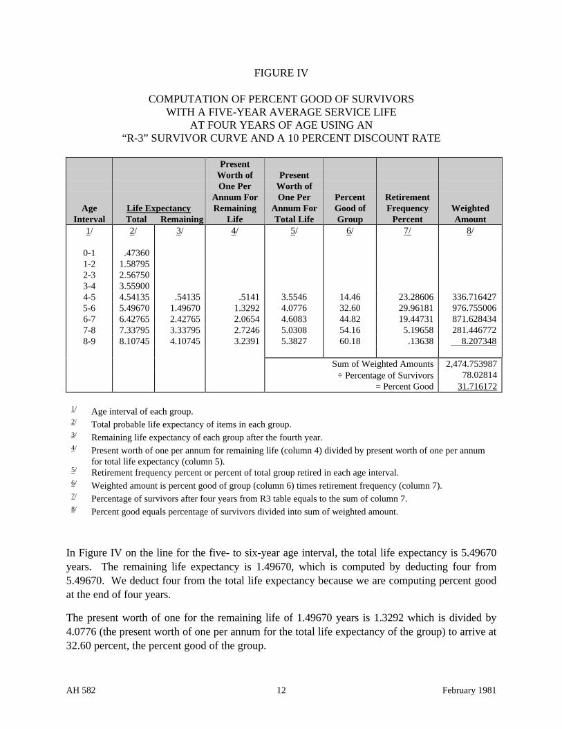
Each factor requires the computation of a series of individual percent good factors for eachsubsequent year and the formulation of a weighted average using the retirement frequency of eachgroup as a weight. Figure IV is an example of the computation of a percent good factor for thefourth year of a table with a five-year average service life expectancy. This computation is alsobased upon an “R-3” retirement frequency curve and a 10-percent discount rate.

In the group method, all items are separated into smaller groups of units that have been retiredwithin each one year age interval. Column one of Figure IV designates the age interval of eachgroup. The average retirement age of each group is then computed. As shown in the table, theaverage age of retirement of the group of units retired in the fifth year of the life of the group is4.54135 years.

A percent good is then computed for each age interval group for each year of the remainingexistence of the group. This is done by dividing the present worth of one per annum for theremaining life expectancy of the group by similarly discounted factor for the total life expectancyof the group.


FIGURE IV

COMPUTATION OF PERCENT GOOD OF SURVIVORSWITH A FIVE-YEAR AVERAGE SERVICE LIFE

AT FOUR YEARS OF AGE USING AN“R-3” SURVIVOR CURVE AND A 10 PERCENT DISCOUNT RATE

PresentWorth of PresentOne Per Worth of

Annum For One Per Percent RetirementAge Life Expectancy Remaining Annum For Good of Frequency Weighted

Interval Total Remaining Life Total Life Group Percent Amount1/

0-11-22-33-44-55-66-77-88-9

2/

.473601.587952.567503.559004.541355.496706.427657.337958.10745

3/

.541351.496702.427653.337954.10745

4/

.51411.32922.06542.72463.2391

5/

3.55464.07764.60835.03085.3827

6/

14.4632.6044.8254.1660.18

7/

23.2860629.9618119.44731

5.19658.13638

8/

336.716427976.755006871.628434281.446772 8.207348

Sum of Weighted Amounts÷ Percentage of Survivors

= Percent Good

2,474.75398778.02814

31.716172

1/ Age interval of each group.2/ Total probable life expectancy of items in each group.3/ Remaining life expectancy of each group after the fourth year.4/ Present worth of one per annum for remaining life (column 4) divided by present worth of one per annum

for total life expectancy (column 5).5/ Retirement frequency percent or percent of total group retired in each age interval.6/ Weighted amount is percent good of group (column 6) times retirement frequency (column 7).7/ Percentage of survivors after four years from R3 table equals to the sum of column 7.8/ Percent good equals percentage of survivors divided into sum of weighted amount.

In Figure IV on the line for the five- to six-year age interval, the total life expectancy is 5.49670years. The remaining life expectancy is 1.49670, which is computed by deducting four from5.49670. We deduct four from the total life expectancy because we are computing percent goodat the end of four years.

The present worth of one for the remaining life of 1.49670 years is 1.3292 which is divided by4.0776 (the present worth of one per annum for the total life expectancy of the group) to arrive at32.60 percent, the percent good of the group.


A percent good for each group still in existence is then computed. A weighted amount iscomputed by multiplying the percent good by the retirement frequency or the percent retiredduring the age interval. All weighted amounts for survivors are summed and divided by thepercentage of survivors to arrive at the percent good.

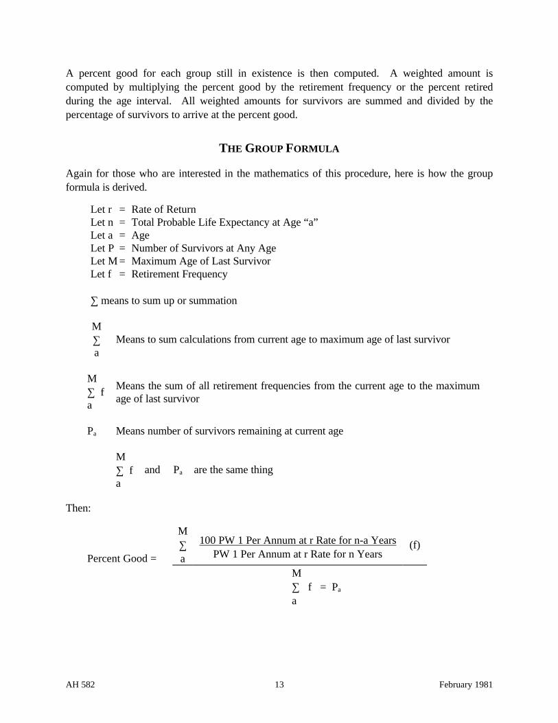
THE GROUP FORMULA

Again for those who are interested in the mathematics of this procedure, here is how the groupformula is derived.

Let r = Rate of ReturnLet n = Total Probable Life Expectancy at Age “a”Let a = AgeLet P = Number of Survivors at Any AgeLet M = Maximum Age of Last SurvivorLet f = Retirement Frequency

∑ means to sum up or summation

M∑ Means to sum calculations from current age to maximum age of last survivora

MMeans the sum of all retirement frequencies from the current age to the maximum∑ fage of last survivor

a

Pa Means number of survivors remaining at current age

M∑ f and Pa are the same thinga

Then:

M100 PW 1 Per Annum at r Rate for n-a Years∑ (f)

PW 1 Per Annum at r Rate for n YearsPercent Good = aM∑ f = Pa

a


M (1 + r)n-a - 1 (1 + r)n - 1∑ 100

r(1 + r)n-a ÷r(1 + r)n (f)

Percent Good = aM∑ f = Pa

a

M(1 + r)n-a - 1 r(1 + r)n

∑ 100r(1 + r)n-a x

(1 + r)n (f) - 1


a

M [(1 + r)n-a - 1)] (1 + r)n

∑ 100 n-a (f)(1 + r) [(1 + r)n - 1)]


a

M (1 + r)a-n [(1 + r)n-a - 1] (1 + r)n

∑ 100 a-n n-a n (f)(1 + r) (1 + r) [(1 + r) - 1]


a

M [(1 + r)a-n + n-a - (1 + r)a-n] (1 + r)n

∑ 100(1 + r)a-n + n-a [(1 + r)n (f)

- 1]Percent Good = a

M∑ f = Pa

a


M [1 - (1 + r)a-n ] (1 + r)n

∑ 100 (f)1 - 1 + rn - 1


a

M (1 + r)n - (1 + r)a-n+n

∑ 100(1 + r)n (f)

- 1Percent Good = a

M∑ f = Pa

a

M (1 + r)n - (1 + r)a

∑ 100(1 + r)n (f)

- 1Percent Good = a

M∑ f = Pa

a


CHAPTER 5: THE EFFECT OF THE FOUR VARIABLES

There are four variables that have an effect on percent good calculations. They are: the rate ofreturn, the method of calculation, the survivor curve, and the income adjustment factor. Whilethe effect of any one variable on the final results is not a major significance, the cumulative effectof all four variables could be devastating. It is important for the users of these tables tounderstand the effect of each variable.

THE EFFECT OF THE YIELD RATE

The first variable in computing percent good factors is the rate of return or yield rate. It is afactor that cannot be calculated precisely because of a lack of data. The best way of estimating aproper return on real property is to analyze the relationship between selling price and anticipatedfuture income. This is done by finding the relationship between the selling price of a recently soldproperty and the buyer’s anticipation of the future income of the property. A relationship isexpressed in terms of a yield rate or capitalization rate that considers a return on outstandingcapital as well as a rate of return of the current value of the wasting assets. It is important thatthe future income projection is in terms of current dollars. It will be usually level or declining andis free of future inflation. (The Property Taxes Department’s objective is to achieve a rate ofreturn that matches an income stream, both being virtually free of inflation.) The sales analysismethod is not often available because industrial properties that are “going” concerns are seldomsold.

For this purpose we must consider several indications and make the most reasonable estimate wecan. One indicator of a yield rate for industrial property can be obtained from the stock and bondmarket. It is called the band of investment method and uses the average rate of return oncommon stocks and the average yield on corporate bond to formulate a rate of return. A goodreference for this data is Standard and Poors Statistical Reference. This publication contains anaverage yield for common stocks and an average yield for 400 “A” rated industrial bonds. TheAugust 31, 1979 average yield for common stocks was 12.5 percent. At the same time theaverage yield on 400 “A” rated bonds was 9.10 percent. A 50-50 weighted average for these twoindicators is 10.8 percent. It is also important when using the band of investment method thatfuture income projections are based upon current dollars, are constant or declining, and thereforereflect inflation free rates of return.

The band of investment method is criticized from the point of view that while it may be applicableto very large, publicly owned corporations it is probably not a good indicator of a proper yield forsmall, singly or closely owned properties. It does, however, provide an indication that ifcombined with other evidence it is possible to make an intelligent estimate of a reasonable yieldrate.


Rates of return derived by the band of investment method reflect a relationship of the net incomeafter all taxes and the value of the fee simple interest in real property. They, therefore, represent arate of return after taxes and do not require a further adjustment.

Interest rates on loans to finance industrial property may also be used. While this does not give usa precise answer, it does give us a general idea of a proper rate. Interest rates on loans are not thesame thing as a rate of return on real property. Loans are secured by a promise to pay while arate of return is secured only by the real property and its earning ability.

Normally, it is expected that interest rates on promissory notes will yield at a lower rate thanequity return. During times of rapid inflation, however, this relationship may be different.Investors may be willing to invest at lower rates in equity positions than they will in fixedpositions. They may feel that inflation will improve their position over time.

While the rate of return is an important factor in percent good calculations, it is not critical. Hereare two examples of differences that arise when an 8 percent and a 10 percent rate are used forcomputing a table. In all cases, an “R-3” survivor curve and the individual method ofcomputation were used.

20-YEAR AVERAGE LIFE

Percent PercentGood At Good At Numerical Percent

Age 8 Percent 10 Percent Difference Difference

5 85.22 87.32 2.10 2.46

10 67.06 70.70 3.64 5.43

15 47.00 51.12 4.12 8.77

20 28.51 31.97 3.46 12.14

25 15.67 18.03 2.36 15.06

10-YEAR LIFE

Percent PercentGood At Good At Numerical Percent

Age 8 Percent 10 Percent Difference Difference

5 58.54 60.67 2.13 3.64

10 21.45 23.09 1.64 7.60

Notice that when the yield rate is increased the percent good is increased. This is just theopposite effect of increasing the capitalization rate in applying the income approach. In theincome approach, the higher the rate of return the lower the value. Here the higher the rate ofreturn the higher the percent good.


It must be remembered that percent good is dependent upon the relationship between the presentworth of one per annum for the total life expectancy and a similar factor for the remaining lifeexpectancy. Present worth factors discounted at low rates are greater than factors discounted athigher rates for the same period of time. For example, the present worth of one per annum for 20years discounted at 8 percent is 9.8181, and the present worth of one per annum for 20 yearsdiscounted at 10 percent is 8.5135. Because the starting point of the income stream discounted at8 percent is higher than the factor arrived at using a 10 percent discount rate, it must declinefaster to reach zero in the same length of time. This more rapid decline pattern produces lowerpercent good factors at the same point in time.

It is interesting to note that variances that will arise from the use of different yield rates in theincome capitalization process will be greater than variances reflected in percent good factorcalculations.

Here is a table showing the differences that arise when an 8 percent yield rate is used as opposedto a 10 percent rate. In both cases, a constant income premise and an income of one are used.Probable remaining life estimates are based upon those derived from an “R-3” survivor curve anda 20-year average service life.

Age

ProbableRemaining Life

ExpectancyPW Factor

At 8 PercentPW Factor

At 10 PercentPercent

Difference

5 15 8.559 7.606 12.5

10 11 7.139 6.495 9.9

15 7 5.206 4.868 6.9

20 4 3.312 3.170 4.5

THE EFFECT OF THE METHOD OF COMPUTATION

The example below shows differences between the individual or average life method and thegroup or unit summation method of computation. It assumes a 20-year life, a 10 percent discountrate, an “R-3” survivor curve, and a 10 percent decline in income over the average life term. Asyou can see, the individual method will produce a slightly higher percent good in the beginningyears. It reaches a peak of 4.51 percent difference at 11 years of age.


DIFFERENCES BETWEEN GROUP AND INDIVIDUAL METHODS

Percent Percent Good Difference in PercentGood Group Individual Percent Good Difference

Age Method Method Factor in Factors

1 97.01 97.77 .76 .8

2 93.97 95.39 1.42 1.5

3 90.83 92.86 2.03 2.2

4 87.58 90.17 2.59 3.0

5 84.24 87.32 3.08 3.7

6 80.79 84.31 3.52 4.4

7 77.26 81.13 3.87 5.0

8 73.65 77.80 4.15 5.6

9 69.97 74.32 4.35 6.2

10 66.23 70.70 4.47 6.7

11 62.45 66.96 4.51 7.2

12 58.62 63.11 4.49 7.7

13 54.77 59.16 4.39 8.0

14 50.92 55.16 4.24 8.3

15 47.09 51.12 4.03 8.6

16 43.30 47.08 3.78 8.7

17 39.61 43.10 3.49 8.8

18 36.04 39.22 3.18 8.8

19 32.64 35.49 2.85 8.7

20 29.45 31.97 2.52 8.6

21 26.50 28.68 2.18 8.2

22 23.78 25.65 1.87 7.9

23 21.31 22.88 1.57 7.4

24 19.06 20.36 1.30 6.8

25 16.99 18.03 1.04 6.1

The reason for the difference is a difference in concept which results in a different calculation. Inthe individual method, the percent good is simply a relationship of the present worth of an income


for the probable remaining life expectancy and one for the total life expectancy. It assumes thatthe best estimate of the future life expectancy of survivors of a group of items is the average ofthe group. All weight is assigned to this single calculation.

The group method assumes that a portion of the group will be retired each year until all areretired. A percent good is calculated for each year, and a weight is assigned for each groupaccording to the number in each group.

THE EFFECT OF THE INCOME ADJUSTMENT FACTOR

The least controversial of the four factors that influence percent good calculations is the incomeadjustment factor. It is generally agreed that income to property tends to decline with time. Theincome adjustment factor used in Assessors’ Handbook Section 581, Equipment Index Factorsand Inventory Ratios, recognizes one adjustment for this factor. The table below shows the effectof this adjustment when a 20-year life, an 8 percent rate, an “R-3” survivor curve, and theindividual method are used to compute the percent good.

Percent Good Percent GoodNo Income With Income Numerical Percentage

Age Adjustment Adjustment Difference Difference

5 89.56 87.32 2.24 2.57

10 74.43 70.71 3.72 5.26

15 55.26 51.12 4.14 8.10

20 35.52 31.97 3.55 11.10

25 20.61 18.03 2.58 14.31

In making this calculation, we are saying that a new property will have an income of one per yearfor its entire life. At the same time, we are saying that the older property will have an income ofsomething less than one for its entire life. To be correct, the income of the newer property shouldequal the income of the older property when it reaches the present age of the older property.

The figures below illustrate the relationship between the income projected for a new property andthat of a 10-year property with a 20-year average service life.

$1.00 20.75 Years $.95 10.75 Years

New Property 10-Year-Old Property


The above is one method of making an adjustment for declining income. Should the net incomedecline at a different rate than indicated by the tables, alterations should be made to the incomeadjustment factors.

THE EFFECT OF THE SURVIVOR CURVE

Here is a table comparing the difference that arises when an “R-3” curve is used as opposed to an“S-3” curve. In both cases, a 10 percent rate of return, a 20-year average service life, theindividual method of computation, and a 10 percent income decline factor are used forcomputation.

Percent Percent GoodGood Using Using “S-3” Percent Percent

Age “R-3” Curve Curve Difference Error

5 85.08 84.88 .20 .24

10 66.98 65.53 1.45 2.21

15 46.97 44.67 2.30 5.15

20 28.42 27.96 .46 1.65

25 15.46 16.63 [1.17] [7.04]

The use of the “R-3” survivor curve has been controversial for some time. The table aboveindicates it has the least effect on the final answer of the variables.

The “R-3” curve was selected because of the pattern of retirements that it reflected. It seemedreasonable to assume that retirements of new items would be few at first; but as machinery andequipment grew older, the effect of wear and tear as well as obsolescence would cause morefrequent retirements. It was felt that the majority of items in any group would reach the averageservice life of the group and possibly survive a little longer, but after this point in time there wouldbe a large number of retirements.

We can probably make an argument that is reasonably valid for using the “S-3” curve. In any caseit seems reasonable that the frequency of retirements is going to be much greater on or near theaverage service life. It follows, then, that an appropriate curve would be an “R-3” or “R-4” ratherthan an “R-1” or “R-2.”

THE USE OF THE PERCENT GOOD FACTORS

Percent good factors contained in Assessors’ Handbook Section 581, Equipment Index Factorsand Inventory Ratios, are based upon a logical premise and follow accepted appraisal practices.They are intended to reflect the average loss in value that commercial and industrial properties, in


general, will suffer over a period of time. The factors are based upon averages and represent areasonable estimate of percent good for the majority of this type property.

In any group of property items, however, there are individual items that deviate from the norm.For example, in the model group that forms the basis for the R-3 survivor curve, 5.5 percent areretired at 50 percent of the average life of the group, and on the other extreme, 3 percent areretired after 145 percent of the average life term of the total group. Items such as these, whoselife terms significantly deviate from the norm, obviously do not closely follow the typical valueloss pattern. Therefore, it is necessary for appraisers to analyze the situation of all property whenpercent good factors are applied. If it is likely that certain property is deviating from the norm,adjustments should be made in the percent good factors.

At the same time, arbitrary deviations from the tables without adequate evidence of deviationsfrom the norm, such as minimum percent good adjustments, are not good appraisal practices. Assurvivors of an original group reach older age, there may be less reliability in percent good factorsapplicable to these items. When property items reach this latter stage of their life and the tablesindicate very low or zero percent good factors for property that is still functioning, specialconsideration should be given in assigning percent good factors.

If for administrative reasons the assessor has established a policy of using minimum percent goodadjustments, he should be prepared to make readjustments if evidence is presented indicating thatthe minimum percent good adjustments are inappropriate.

Since percent good factors are not computed according to causes of depreciation, it is impossibleto quantify the portion of the indicated value loss that is due to the various causes. However, wecan say that the factors include a normal amount of physical deterioration, normal functionalobsolescence, and, to the extent that it is normal, normal economic obsolescence.

Assessors' Handbook Section 582, The Explanation … present worth factor for the total life of the...

Documents

Transcript of Assessors' Handbook Section 582, The Explanation … present worth factor for the total life of the...