AssessmentofTwo-EquationTurbulenceModelsand ...downloads.hindawi.com/archive/2012/428671.pdf ·...

International Scholarly Research NetworkISRN Mechanical EngineeringVolume 2012, Article ID 428671, 10 pagesdoi:10.5402/2012/428671

Research Article

Assessment of Two-Equation Turbulence Models andValidation of the Performance Characteristics of anExperimental Wind Turbine by CFD

Ece Sagol,1 Marcelo Reggio,1 and Adrian Ilinca2

1 Ecole Polytechnique de Montreal, 2500 Chemin de Polytechnique, Montreal, QC, Canada H3T 1J42 Universite du Quebec a Rimouski (UQAR), 300, Allee des Ursulines, Rimouski, QC, Canada G5L 3A1

Correspondence should be addressed to Ece Sagol, [email protected]

Received 7 September 2011; Accepted 27 October 2011

Academic Editors: A. Z. Sahin and B. Yu

Copyright © 2012 Ece Sagol et al. This is an open access article distributed under the Creative Commons Attribution License,which permits unrestricted use, distribution, and reproduction in any medium, provided the original work is properly cited.

The very first step in the simulation of ice accretion on a wind turbine blade is the accurate prediction of the flow field aroundit and the performance of the turbine rotor. The paper addresses this prediction using RANS equations with a proper turbulencemodel. The numerical computation is performed using a commercial CFD code, and the results are validated using experimentaldata for the 3D flow field around the NREL Phase VI HAWT rotor. For the flow simulation, a rotating reference frame method,which calculates the flow properties as time-averaged quantities, has been used to reduce the time spent on the analysis. A basicgrid convergence study is carried out to select the adequate mesh size. The two-equation turbulence models available in ANSYSFLUENT are compared for a 7 m/s wind speed, and the one that best represents the flow features is then used to determinemoments on the turbine rotor at five wind speeds (7 m/s, 10 m/s, 15 m/s, 20 m/s, and 25 m/s). The results are validated againstexperimental data, in terms of shaft torque, bending moment, and pressure coefficients at certain spanwise locations. Streamlinesover the cross-sectional airfoils have also been provided for the stall speed to illustrate the separation locations. In general, resultshave shown good agreement with the experimental data for prestall speeds.

1. Introduction

Prediction of the aerodynamic loads on a horizontal axiswind turbine (HAWT) is both an important and a complexprocess that takes place during the design stage. It is impor-tant because it is directly related to crucial characteristicsof the wind turbine, such as its power curve, structuralloads, and noise generation. The power curve determinesthe energy output of the wind turbine, and therefore itscost effectiveness, structural loads determine the size of thevarious wind turbine components and materials to be used,and noise generation is a consideration for the location of awind turbine and should be kept to a reasonable level. Thecomplexity of a flow simulation around a wind turbine bladeto determine aerodynamic loads comes from large angles ofattack, a variety of Reynolds numbers resulting from verylong blades, and rotational effects. Further complicating theissue is the atmospheric boundary layer, variable wind speeds

along the blade, and interaction of the rotor with the nacelleand the tower.

Although 2D and quasi-3D methods like blade elementmomentum analysis may predict aerodynamic loads up toa certain level, 3D analysis is required to capture all theturbulence features that are inherently three dimensional. Ascomputational cost drops thanks to technological develop-ment, the use of computational fluid dynamics (CFD) forwind turbine design and analysis is becoming increasinglywidespread and results in a better understanding of theaerodynamic phenomena on the rotor flow field.

Studies on wind turbine aerodynamics in the literaturefocus on different aspects of the science, like performanceanalysis, fluid-structure interaction, acoustics, and icing.Investigation into performance analysis is primarily aimedat estimating aerodynamic loads, and the effect of variousparameters on these loads. Duque et al. [1] explored theability of various methods to predict wind turbine power

2 ISRN Mechanical Engineering

and aerodynamic loads. Results showed that all the methods,namely blade element momentum (BEM), vortex lattice,and reynolds averaged navier stokes (RANS), perform wellfor prestall regimes. They found that the RANS codeOVERFLOW, although not perfect, gives better predictionsof power production for stall and poststall regime modelingthan other methods. Another study, based on CFD analysis(Sorensen et al. [2]), showed that performance and windturbine load predictions are very accurate, except in the stallregion. A commercial wind turbine company, Siemens, ana-lyzed their own large-scale wind turbine using a commercialCFD code, ANSYS-CFX, with transition and fully turbulentmodels [3]. Transition models improve drag prediction butoverestimate the lift compared to fully turbulent models.Benjanirat et al. [4] used CFD with various turbulencemodels (Boldwin-Lomax, Spalart-Allmaras, and k-ε), withand without wall corrections, on an experimental windturbine. The k-ε model with wall correction yielded thebest results when compared with experimental data. A morerecent study, conducted by Sezer-Uzol and Long [5] using ageneric CFD code, PUMA2, have shown that time accurateinviscid results are also compatible with the experimentaldata.

Predicting the effects of tower, nacelle, and anemometeron the rotor flow field have also been investigated in severalworks. Smaili and Masson [6] and Zahle and Sorensen [7]both concluded that CFD is an effective tool for evaluatingthe influence of the nacelle, even for different positions andalignments of the wind turbine blade. A successful study ofthe interaction between rotor and tower [8] emphasizes theimportance of CFD in solving complex flow phenomena.All these studies show that, even though CFD requiresmore resources for unsteady problems, it is cheaper thanconducting full-scale or scaled wind turbine experimentalanalysis but yet provides sufficiently accurate results. Byimproving its capability to simulate widely separated flowsthrough better turbulence modeling near the wall and inthe flow field, CFD tools are becoming more and moreaccurate for the aerodynamic and aeroelasticity analysis ofwind turbine blades.

Even though the final objective of the current study isto perform icing simulation on wind turbine blades, thecharacteristics of the flow field and the integrated loads ofthe clean blade are nevertheless required. To obtain thesedata, a grid study is performed to represent the flow fieldaccurately with a minimum grid size. Three different grids,with 1.6 M, 1.9 M, and 2.2 M cells, are tested using thecommercial CFD code (ANSYS-FLUENT [9]) at a prestallspeed of 7 m/s and the results compared with experimentaldata. Once the grid convergence analysis has been conducted,various two-equation turbulence models are tested to findthe one that best fits the experimental NREL Phase VI HAWTresults. Thus, for each turbulence model, standard k-ε, RNGk-ε, realizable k-ε, and SST k-ω simulations are performedat a wind speed of 7 m/s, characterized by a reduced stallregion on the rotor blade, to obtain pressure distributionsand integrated aerodynamic loads on the blade. Results arecompared with experimental data to find the most suitableturbulence model. Once that model has been selected, new

Table 1: NREL phase VI experimental wind turbine characteristics.

Number of blades 2

Diameter 5.029 m

Airfoil S809

Root chord 0.7366 m

Tip chord 0.3808 m

Root twist 21.8◦

Tip twist −1.775◦

Rotational speed 72 rpm

0

5

10

15

20

25

0 0.2 0.4 0.6 0.8 1−5

TW

IST

(de

g)

r/R

(a)

0 0.2 0.4 0.6 0.8 10

0.2

0.4

0.6

0.8C

HO

RD

(m

)

r/R

(b)

Figure 1: (a) Twist distribution; (b) chord distribution.

simulations are performed throughout the operational windspeed range of the wind turbine.

2. Methodology

2.1. Experimental Data. For this study, we selected oneof the unsteady aerodynamics experiments (UAEs), theNREL Phase VI wind turbine, conducted by the NationalRenewable Energy Laboratory (NREL) in the NASA-Ameswind tunnel at Moffett Field, California, in 2000 [10, 11]. TheNREL organized the data used in this paper. The advantageof using a wind tunnel of such gigantic proportions (24.4 mby 36.6 m, or 80 ft by 120 ft) to perform a full scale 10 mdiameter wind turbine test is that the blockage effect is notsignificant.

The general characteristics of the NREL Phase VI windturbine are given in Table 1. The S809 airfoil is used for theentire blade. Linear chord and nonlinear twist distributionsare shown in Figure 1. The blade root is completely circularup to 0.883 m, and, from this point up to 1.2573 m, the shapesmoothly transforms from a circle into an airfoil configura-tion. The 3D CAD model of the blade was generated usingthe commercial software Rhinoceros 4.0 [12]. Figure 2 showsthe geometry.

ISRN Mechanical Engineering 3

(a)

y

x

(b)

Figure 2: 3D CAD model of the NREL phase VI experimental windturbine.

From the experimental data, the upwind, 3◦ pitch, andnonyaw configurations were selected as validation data. Theexperimental parameters to be validated are the pressurecoefficients at pressure tap locations (30%, 46.6%, 63.3%,80%, and 95% span), the low-speed shaft torque, and thebending moment on the blade throughout the operationalwind speed range. The experimental data are provided for a30 second time period, and time-averaged data are used forthe comparison.

For the selected data, the wind turbine rotation directionis counter-clockwise when viewed from upwind. The coneangle is 0◦. The rotor speed is 72 rpm, and the pitch angle is3◦. The pitch angle is defined at 75% of the span, 0.75R, andthe pitch axis is given as 30% of the chord, 0.3c.

2.2. Numerical Study. Today, CFD tools, whether commer-cial or developed inhouse, are routinely used for investigatingthe aerodynamics and fluid-structure interactions aroundnumerous configurations. Of the commercial tools available,ANSYS FLUENT 12.0.16 is used in the current study.The package is a finite volume-based solver, which allowsboth structured and unstructured grids to discretize thecomputational domain [9]. The software allows transientcalculations as well as steady-state computations to beperformed. Parallel computation capabilities are also offeredto handle large meshes and to reach solutions in a reasonabletime.

For this study, an incompressible, steady, Reynolds-averaged Navier Stokes (RANS) model is applied to solvethe problem on a “rotating reference frame.” The basic ideabehind the rotating reference frame is the assumption thatit is the flow field that rotates, and not the rotor, whichmeans that an unsteady flow field turns into a steady flowwith respect to the rotating reference frame. This approachsimplifies the problem in terms of boundary conditions(no sliding mesh is required), computational cost, andpostprocessing results.

To reduce the complexity of the problem and the timespent on computational analysis, we made a number ofhypotheses prior to numerical analysis. Initially, effects of thetower and the nacelle are ignored to reduce mesh size andthe complexity of the problem. Although they may affect theperformance and flow field of the rotor, they are neglected inmany studies when they are not the focus of the research [1–4]. Moreover, on the assumption that the flow field is 180◦

axisymmetric, one blade is modeled instead of two, and a“rotational periodic” boundary condition is applied, in orderto reduce the computational cost. As explained above, sincethe blockage effect of the wind tunnel is minimal, the windtunnel walls are not taken into account in the numericaldomain. Finally, although the experimental data are timedependent, numerical analysis is conducted at steady statewith the rotating reference frame model, which predictstime-averaged quantities. As a result, the time-averagedquantities of the experimental data and the numerical resultscan be compared.

Two-equation turbulence models have been widely usedto simulate the flow field in engineering applications. Asthe name implies, these models have two independenttransport equations, one for turbulent kinetic energy, and theother for turbulent dissipation or specific dissipation rate.Two equation models are complete, which means that noadditional equations are needed to model the turbulence,and that they both depend on the Boussinesq assumption[13]. Details of turbulence models that are applied in thisstudy are briefly explained below.

2.2.1. Standard k-ε Turbulence Model. The transport equa-tions of the k-ε models are based on the turbulent kineticenergy, k, and the dissipation rate, ε. The simplest, thestandard k-ε model, proposed by Launder and Spalding [14],is based on the assumption that flow is fully turbulent.This model gives better results for fully turbulent flows. Thetransport equations for the standard k-ε model are as follows:

∂

∂xi

(ρkui

) = ∂

∂xj

[(μ +

μtσk

)∂k

∂xj

]

− ρu′ι u′j

∂uj

∂xi− ρε + Sk,

∂

∂xi

(ρεui

) = ∂

∂xj

[(μ +

μtσε

)∂ε

∂xj

]

− C1εε

kρu′ι u

′j

∂uj

∂xji− C2ερ

ε2

k+ Sε.

(1)


The turbulent viscosity is calculated using k and ε as follows:

μt = ρCμk2

ε. (2)

The model coefficients, which are empirically determined,are given as in [14]:

C1ε = 1.44, C2ε = 1.92,Cμ = 0.09, σk = 1.0, σε = 1.3.(3)

2.2.2. RNG k-ε Turbulence Model. A more developed k-ε tur-bulence model, RNG k-ε, which is based on renormalizationgroup theory [15], has correction terms for swirling flow, lowReynolds number flow, and flow with high velocity gradients.The transport equations of the RNG k-ε model are verysimilar to those of the standard k-ε model, except as shownbelow:

∂

∂xi

(ρkui

) = ∂

∂xj

[

αkμeff∂k

∂xj

]

− ρu′ι u′j

∂uj

∂xi− ρε + Sk,

(4)

∂

∂xi

(ρεui

) = ∂

∂xj

[

αkμeff∂ε

∂xj

]

− C1εε

kρu′ι u

′j

∂uj

∂xi− C∗2ερ

ε2

k+ Sε,

(5)

where

C∗2ε = C2ε+Cμη3

(1− η/η0

)

1 + βη3η = S

k

εη0 = 4.38 β = 0.012.

(6)

The model coefficients, which are derived analytically byRNG, are given as in [15]:

C1ε = 1.42 C2ε = 1.68. (7)

As can be seen from (5), the coefficient of dissipation termC∗2ε is modified to provide better adaptability of the modelto rapid strained flows [9]. Moreover, the effective viscosityterm μeff in both transport equations improves the model forlow Reynolds numbers and near-wall regions. For swirledflows, the RNG k-ε model of ANSYS FLUENT [9] has anoptional correction model that calculates turbulent viscosityas a function of swirl strength. For this study, the swirlcorrection is enabled as the flow field rotates.

2.2.3. Realizable k-ε Turbulence Model. The realizable k-εmodel, proposed by Shih et al. [16], is a new turbulent

viscosity model that accounts for rotation and strain in theflow. The transport equations of the model are the following:

∂

∂xi

(ρkui

) = ∂

∂xj

[(μ +

μtσk

)∂k

∂xj

]

− ρu′i u′j

∂uj

∂xi− ρε + Sk,

∂

∂xi

(ρεui

) = ∂

∂xj

[(μ +

μtσε

)∂ε

∂xj

]

+ ρC1Sε

− ρC2ε2

k +√

νε− Sε,

(8)

where

C1 = max

[

0.43,η

η + 5

]

η = Sk

εS =

√2Si jSi j . (9)

The realizable k-ε model is significantly different from otherk-ε models, in that the turbulent viscosity coefficient Cμ

depends on mean strain and rotation rates, turbulent kineticenergy, and energy dissipation, the use of which ANSYSFLUENT recommends for better prediction of the turbulentviscosity [9]. The model coefficients of the realizable k- εmodel are given as in [9]:

C1ε = 1.44 C2 = 1.9 σk = 1.0 σε = 1.2. (10)

2.2.4. SST k-ω Turbulence Model. This model, which waspresented by Menter [17], is a combination of the standardk-ω model and the transformed k-ε model. It benefits fromthe advantages of both these turbulence models in differentflow regions, activating the standard k-ω model near the walland the k-ε model away from the surface. The SST k-ω modelhas been found to be more accurate than other turbulencemodels [9]

∂

∂xi

(ρkui

) = ∂

∂xj

[

Γk∂k

∂xj

]

+ Gk − ρβ∗kω + Sk,

∂

∂xi

(ρωui

) = ∂

∂xj

[

Γω∂ω

∂xj

]

+α

νtGk − ρβω2

+ 2(1− F1)ρσω,21ω

∂k

∂xj

∂ω

∂xj+ Sω,

(11)

where the term Gk is

Gk = min

(

−ρu′ι u′j∂uj

∂xi, 10ρβ∗kω

)

. (12)

The model coefficients are given as in [9]:

σk = 1.176 σω = 2.0 (13)

2.2.5. Computational Domain. The geometries of the windturbine and the domain for the numerical analysis aregenerated using Rhinoceros [13]. Figure 3 illustrates thecomputational domain. The inlet and outlet boundaries


Inlet3D

Periodic

5DOutlet

Mesh refinement region

Figure 3: Computational domain for the NREL Phase VI rotor.

are placed at 3 times and 5 times the diameter from thewind turbine, respectively. Since an axisymmetric flow fieldis required for using the rotating reference frame and therotational periodic boundary condition, a semicylindricaldomain has been generated. To improve accuracy, a secondsmall semicylindrical domain around the blade has also beengenerated, in order to refine the mesh in this region, asillustrated in Figure 3.

An unstructured mesh was chosen for the domain dis-cretization. The surface mesh was generated using GAMBIT,formerly the companion software of FLUENT. For thesurface mesh, the size functions of GAMBIT that enable theuser to control the grid distribution over the surface wereused. The number of nodes was maximized near the leadingedge, where the large pressure gradients exist. “Meshed” sizefunctions provided smooth transactions of mesh size fromedges to face, whereas “curvature” size functions providedbetter representation of curved surfaces by keeping the meshsize to a minimum, as seen in Figure 4(a). To resolve theboundary layer, 20 prism layers normal-to-surface elementson the blade were generated. The initial height selected was10−5 m, which guarantees y + < 10 on the blade surface. Threedifferent grids with mesh sizes of 1.6 M, 1.9 M, and 2.2 Mwere used. The surface mesh and prism layer are shown inFigures 4(a) and 4(b), respectively.

2.2.6. Boundary Conditions. For the inlet boundary condi-tion, the velocity normal to the inlet boundary and theturbulence intensity, which are provided by experimentaldata, were imposed. The outer cylindrical domain is alsotreated as an inlet, and the same boundary conditionsare applied. For the outflow boundary, the pressure outletboundary condition is enforced by applying atmosphericpressure, as the flow is far from the wind turbine. Forthe inner surfaces, as explained above, rotational periodicboundary conditions are applied. Finally, the blade surfacewas treated as a no-slip wall boundary condition; that is, azero velocity is imposed.

3. Results

In this section, results of the comparison of 3D numericalstudies and the UAE data [11] are presented, starting withthe results of the grid optimization study. To find the mostconvenient turbulence model, various two-equation turbu-lence models available in ANSYS FLUENT were applied, and

(a)

(b)

Figure 4: (a) Surface triangular mesh, (b) domain tetrahedral andprism mesh.

the pressure coefficients were compared with the UAE data.The models that are available in the software are standard k-ε,RNG k-ε, realizable k-ε, standard k-ω, and SST k-ω. Initially,the results of these comparisons are presented for a 7 m/swind speed and preselected spanwise locations, as explainedin the Section 2. As will be shown below, the k-ω SSTturbulence model fits the UAE data better, and so this modelwas selected for the rest of simulations at higher wind speeds.To further verify the numerical study, moments on the windturbine blade, that is, low speed shaft torque and root flapmoment, were compared. Finally, the numerical tool’s abilityto predict separated flow was shown by comparing prestalland stall velocity simulations.

3.1. Grid Study. To ensure the accuracy of the results andto keep the computational cost to a minimum, a basic


(a)

(b)

z yx

(c)

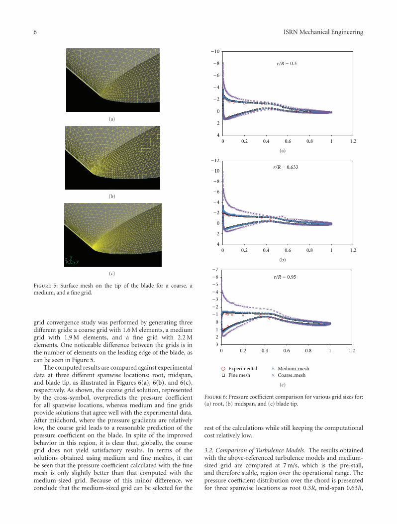
Figure 5: Surface mesh on the tip of the blade for a coarse, amedium, and a fine grid.

grid convergence study was performed by generating threedifferent grids: a coarse grid with 1.6 M elements, a mediumgrid with 1.9 M elements, and a fine grid with 2.2 Melements. One noticeable difference between the grids is inthe number of elements on the leading edge of the blade, ascan be seen in Figure 5.

The computed results are compared against experimentaldata at three different spanwise locations: root, midspan,and blade tip, as illustrated in Figures 6(a), 6(b), and 6(c),respectively. As shown, the coarse grid solution, representedby the cross-symbol, overpredicts the pressure coefficientfor all spanwise locations, whereas medium and fine gridsprovide solutions that agree well with the experimental data.After midchord, where the pressure gradients are relativelylow, the coarse grid leads to a reasonable prediction of thepressure coefficient on the blade. In spite of the improvedbehavior in this region, it is clear that, globally, the coarsegrid does not yield satisfactory results. In terms of thesolutions obtained using medium and fine meshes, it canbe seen that the pressure coefficient calculated with the finemesh is only slightly better than that computed with themedium-sized grid. Because of this minor difference, weconclude that the medium-sized grid can be selected for the

0

2

40 0.2 0.4 0.6 0.8 1 1.2

−10

−8

−6

−4

−2

= 0.3r/R

(a)

0

2

40 0.2 0.4 0.6 0.8 1 1.2

−10

−8

−6

−4

−2

= 0.633−12

r/R

(b)

0 0.2 0.4 0.6 0.8 1 1.2

= 0.95

0

−7

−6

−5

−4

−3

−2

−1

1

2

3

ExperimentalFine mesh

Medium meshCoarse mesh

r/R

(c)

Figure 6: Pressure coefficient comparison for various grid sizes for:(a) root, (b) midspan, and (c) blade tip.

rest of the calculations while still keeping the computationalcost relatively low.

3.2. Comparison of Turbulence Models. The results obtainedwith the above-referenced turbulence models and medium-sized grid are compared at 7 m/s, which is the pre-stall,and therefore stable, region over the operational range. Thepressure coefficient distribution over the chord is presentedfor three spanwise locations as root 0.3R, mid-span 0.63R,


0 0.2 0.4 0.6 0.8 1 1.2

= 0.3

0

−4

−3

−2

−1

1

2

r/R

(a)

0 0.2 0.4 0.6 0.8 1 1.2

= 0.633

0

−4

−3

−2

−1

1

2

3

0.60.8

11.2

−2

−2.5

−1.5

r/R

(b)

Experimentalkw-SSTkeps real

keps RNGkeps STD

0 0.2 0.4 0.6 0.8 1 1.2

r/R = 0.95

3.53

2.52

1.51

0

−0.5

−1.5

−2

0.5

−1

(c)

Figure 7: Comparison of pressure coefficients for various turbu-lence models against experimental data for: (a) root, (b) midspan,and (c) blade tip.

and tip 0.95R. The pressure coefficient is obtained by (14),where W represents the wind speed, rΩ is the local rotationalspeed at that spanwise location, and c indicates the localchord. Comparison of the calculations obtained with thevarious turbulence models against experimental data areshown in Figures 7(a)–7(c)

Cp = P∞ − P0

(1/2)ρ(W2 + (rΩ)2

) . (14)

0

0.2

0.4

0.6

0.8

1

1.2

1.4

1.6

1.8

2

5 10 15 20 25

Low speed shaft torque

CFDExperimental

Wind speed (m/s)

LSST

(kN·m

)

(a)

0

0.5

1

1.5

2

2.5

3

3.5

4

4.5

5Root flap bending moment

5 10 15 20 25

CFDExperimental

Wind speed (m/s)

RFB

M (

kN·m

)

(b)

Figure 8: Comparison of experimental data and CFD results for:(a) low-speed shaft torque; (b) root flap bending moment.

At first glance, with the exception of the standard k-ε model,all the turbulence models seem to predict the pressurecoefficient well at the pressure side and at the suction side.The standard k-ε model overestimates the pressure at theleading edge.

At the root of the blade (Figure 7(a)), where the rota-tional speed is relatively very low, the compatibility of all theturbulence models seems good. However, if the results areevaluated in detail at the leading edge and tip of the section,differences among the models become clearer. As seen indetail in Figure 7(a), the pressure coefficient predicted withthe SST k-ω model is the best when compared with theexperimental data, and the computed pressure coefficient isthe worst when using the standard k-ε model.

At the mid-span location (Figure 7(b)), the calculationswith the standard k-ε model further deviate from theexperimental data at the leading edge of the blade. Thedetailed comparisons of the pressure coefficients are shownat both the suction and pressure surfaces of the leading edge.The results of the other models are close at this location.


051015202530354045505560

Rel-velocity-magnitude

Figure 9: Streamlines over the blade and relative velocity distribution at 0.3R, 0.466R, 0.633R, 0.8R, and 0.95R.

The ability of a turbulence model to accurately simulateflow becomes evident at the tip of the blade, where therotational speed is the highest. As seen from the details inFigure 7(c), the predictions provided by the SST k-ω modelare closer to the experimental data, and those obtained withthe standard k-ε model deviate the most. Moreover, it isworth noting that the differences between the computationsperformed with the realizable k-ε and RNG k-ε models arevery small, and these solutions appear to be the same inFigure 7(a)–7(c). Although there is no separation at all atthis location at 7 m/s, the prediction capability of all theturbulence models decreases visibly compared to that at theroot and mid-span locations.

As a result, among the turbulence models, the best overallcompatibility with experimental data is shown by the SSTk-ω model for all spanwise locations. Similar conclusionshave been drawn by Villalpando et al. [18, 19], who analyzedthe flow over an NACA 63415 airfoil and showed thatalthough all the turbulence models predict the lift, drag,and pressure coefficients well, the k-ω SST model providesa better estimate of the vortex shedding patterns of the flow.

3.3. Comparison of Moments on the Blade. Using a medium-sized grid and the SST k-ω model, a number of simulationswere performed to predict the integrated loads on the rotorthrough the operational wind speed interval of the wind tur-bine at 7 m/s, 10 m/s, 15 m/s, 20 m/s, and 25 m/s. Momentson the blade, namely, low speed shaft torque (LSST) androot flap bending moment (RFBM), are compared againstUAE data over the operational wind speeds, as shown inFigures 8(a) and 8(b). Figure 8(a) reveals that the numericalstudy underpredicts the LSST by up to 20% comparedwith the UAE data, except at the 10 m/s stall speed, wherethe LSST is underpredicted by about 40%. In spite of thelarge deviation, numerical torque exhibits the same trendas the UAE data. The rather poor compatibility of theLSST data is attributed to the drag, that is, the dominantcontribution to the LSST, especially at low wind speedsand for low CFD prediction capability for widely separatedflows, as mentioned in Section 1. In contrast to LSST, RFBMcomparison shows fairly good compatibility with the UAEdata, as shown in Figure 8(b).

Streamlines over the blade and the velocity field atspanwise locations 0.3R, 0.466R, 0.633R, 0.8R, and 0.95R

are given for 10 m/s in Figure 9, which shows that the flowis widely separated at mid-board locations. Separation overthe blade affects the accuracy of the prediction of forcesadversely, as mentioned above. Comparison of the pressurecoefficients against experimental data at 10 m/s is shownin Figures 10(a)–10(e). It can be seen that the pressurecoefficients are not as well predicted as in the 7 m/s test case.The effect of separation can be clearly seen at the suctionsurfaces 0.466R, 0.633R, and 0.8R, where there are separationbubbles. In fact, at each spanwise location, prediction of thepressure coefficient at the suction side is less accurate thanthat obtained on the pressure side.

4. Concluding Remarks

Performance of the NREL Phase VI experimental windturbine rotor has been simulated using the commercial CFDtool ANSYS FLUENT. The simulation conditions selectedwere an upwind turbine configuration with 0◦ yaw and3◦pitch alignment. For the simulations, a rotating referenceframe model is used. A grid with 1.9 million elements wasselected through a grid optimization study. For handlingturbulence, the two-equation models available in ANSYSFLUENT were used for 7 m/s, and the k-ω SST model wasfound to be the most appropriate.

The resultant moments obtained through the operationalwind speed range (7, 10, 15, 20, and 25 m/s) were comparedagainst experimental data. The comparison of momentsshows good agreement, especially for the RFBM. Althoughthe LSST results deviate from the experimental data in the20% range, the trend similar to that of the experimental data.Comparisons of pressure coefficients for stall speed (10 m/s)were presented for five different spanwise locations. Theadverse effects of separation on prediction capability havebeen shown. However, as mentioned above, the capability ofthe CFD method to simulate highly separated flows remainspoor. Moreover, the major deviation from the experimentaldata for the leading edge, caused by the large pressuregradients, is a problem that can be addressed by increasingthe grid density in this region.

Although the current results can only be seen as pre-liminary, the flow field data and the velocity and pressuredistributions obtained will serve as initial data for themultiphase analysis of air and water that is required for icing


0

2

40 0.2 0.4 0.6 0.8 1 1.2

−8

−6

−4

−2

= 0.3r/R

(a)

0 0.2 0.4 0.6 0.8 1 1.2

= 0.466

0

2

4

−6

−4

−2

−5

−3

−1

1

3

r/R

(b)

0

2

40 0.2 0.4 0.6 0.8 1 1.2

−8

−6

−4

−2

= 0.633r/R

(c)

0 0.2 0.4 0.6 0.8 1 1.2

= 0.8

0

2

4

−4

−2

−5

−3

−1

1

3

r/R

(d)

0 0.2 0.4 0.6 0.8 1 1.2

= 0.95

0

2

−2

−3

−1

1

−2.5

−1.5

−0.5

0.5

1.5

r/R

(e)

Figure 10: Pressure coefficient comparison at stall speed, 10 m/s, for: (a) 0.3R, (b) 0.466R, (c) 0.633R, (d) 0.8R, and (e) 0.95R.

simulation. In a subsequent work, calculations at variouswind speeds will be conducted on an iced wind turbine blade,and the performance of the blade will be compared with thatof the clean blade presented in this study.

Symbols and Abbreviations

K : Turbulent kinetic energy per mass (J/kg)P0: Atmospheric pressure (Pa)P∞: Static pressure (Pa)r: Radial location (m)R: Radius of the wind turbine (m)

Sk, Sε, Sω: User-defined source terms for turbulentkinetic energy, dissipation rate, and specificdissipation rate, respectively

Si j : Mean rate-of-strain tensor (s−1)t: Time (s)ui: Flow velocity component (m/s)u′ι u

′j : Reynolds stress tensor

W : Wind speed (m/s)ε: Turbulence dissipation rate (m2/s3)μ: Dynamic viscosity (Pa-s)μt: Turbulent viscosity (Pa-s)ν: Kinematic viscosity (m2/s)


ρ: Density of the air (kg/m3)ω: Specific dissipation rate (s−1)Ω: Angular speed (rad/s)HAWT: Horizontal axis wind turbineLSST: Low speed shaft torqueNREL: National renewable energy laboratoryUAE: Unsteady aerodynamics experiment.

Acknowledgment

E. Sagol expresses her gratitude to WesNET for their financialsupport and to Scott Schreck of the NREL for the experimen-tal data.

References

[1] E. Duque, W. Johnson, J. P. vanDam, R. Cortes, and K. Yee,“Numerical predictions of wind turbine power and aerody-namic loads for the NREL phase II combined experimentalrotor,” in Proceedings of the AIAA/ASME Wind Energy Sympo-sium AIAA 38th Aerospace Sciences Meeting, Reno, Nev, USA,January 2000.

[2] N. N. Sorensen, J. A. Michelsen, and S. Schreck, “Navier-stokesprediction of the NREL phase VI rotor in the NASA ames 80 ftx 120 ft wind tunnel,” Wind Energy, vol. 5, pp. 151–169, 2002.

[3] J. Laursen, P. Enevoldsen, and S. Hijort, “‘3D CFD quantifi-cation of the performance of a multi-megawatt wind turbine,’the science of making torque from wind,” Journal of PhysicsConference Series, vol. 75, Article ID 012007, 2007.

[4] S. Benjanirat, L. N. Sankar, and G. Xu, “Evaluation of turbu-lence models for the prediction of wind turbine aerodynam-ics,” in Proceedings of the ASME 2003 Wind Energy Symposium(WIND ’03), no. AIAA-2003-0517, pp. 73–83, Reno, Nev,USA, January 2003.

[5] N. Sezer-Uzol and L. N. Long, “3-D time-accurate CFDsimulations of wind turbine rotor flow fields,” in Proceedingsof the 44th AIAA Aerospace Sciences Meeting and Exhibit, AIAApaper 2006-394, pp. 4620–4642, Reno, Nev, USA, January2006.

[6] A. Smaili and C. Masson, “On the rotor effects upon nacelleanemometry for wind turbines,” Wind Engineering, vol. 28, no.6, pp. 695–714, 2004.

[7] F. Zahle and N. Sorensen, “Characterization of the unsteadyflow in the nacelle region of a modern wind turbine,” WindEnergy, vol. 14, no. 2, pp. 271–283, 2011.

[8] F. Zahle, N. N. Sørensen, and J. Johansen, “Wind turbinerotor-tower interaction using an incompressible overset gridmethod,” Wind Energy, vol. 12, no. 6, pp. 594–619, 2009.

[9] ANSYS fluent 12.0 theory guide.[10] M. M. Hand, D. A. Simms, L. J. Fingersh et al., “Unsteady

aerodynamics experiment phase VI: wind tunnel test config-urations and available data campaigns,” NREL report numberNREL/TP-500-29955, 2001.

[11] D. A. Simms, S. Schreck, M. M. Hand, and L. J. Fingersh,“NREL unsteady aerodynamics experiment in the NASA-Ames wind tunnel: a comparison of predictions to measure-ments,” NREL report number NREL/TP-500-29494, 2001.

[12] “Rhinoceros NURBS modelling for windows, version 4.0,”User’s Guide.

[13] D.C. Wilcox, Turbulence Modeling for CFD, DCW Industries,Le Canada, Calif, USA, 1994.

[14] B. E. Launder and D. B. Spalding, Lectures in MathematicalModels of Turbulence, Academic Press, London, UK, 1972.

[15] V. Yakhot and S. A. Orszag, “Renormalization group analysisof turbulence. I. Basic theory,” Journal of Scientific Computing,vol. 1, no. 1, pp. 3–51, 1986.

[16] T.-H. Shih, W. W. Liou, A. Shabbir, Z. Yang, and J. Zhu, “Anew k-epsilon eddy viscosity model for high reynolds numberturbulent flows,” Computers and Fluids, vol. 24, no. 3, pp. 227–238, 1995.

[17] F. R. Menter, “Two-equation eddy-viscosity turbulence modelsfor engineering applications,” AIAA Journal, vol. 32, no. 8, pp.1598–1605, 1994.

[18] M. Reggio, F. Villalpando, and A. Ilinca, “Assessment of tur-bulence models for flow simulation around a wind turbineairfoil,” Modelling and Simulation in Engineering, vol. 2011,Article ID 714146, 8 pages, 2011.

[19] F. Villalpando, M. Reggio, and A. Ilinca, “Numerical study offlow around an iced wind turbine airfoil,” submitted to Journalof Engineering Applications of Computational Fluid Mechanics.

International Journal of

AerospaceEngineeringHindawi Publishing Corporationhttp://www.hindawi.com Volume 2010

RoboticsJournal of

Hindawi Publishing Corporationhttp://www.hindawi.com Volume 2014


Active and Passive Electronic Components

Control Scienceand Engineering

Journal of



RotatingMachinery


Hindawi Publishing Corporation http://www.hindawi.com

Journal ofEngineeringVolume 2014

Submit your manuscripts athttp://www.hindawi.com

VLSI Design



Shock and Vibration


Civil EngineeringAdvances in

Acoustics and VibrationAdvances in



Electrical and Computer Engineering

Journal of

Advances inOptoElectronics

Hindawi Publishing Corporation http://www.hindawi.com

Volume 2014

The Scientific World JournalHindawi Publishing Corporation http://www.hindawi.com Volume 2014

SensorsJournal of


Modelling & Simulation in EngineeringHindawi Publishing Corporation http://www.hindawi.com Volume 2014


Chemical EngineeringInternational Journal of Antennas and

Propagation




Navigation and Observation



DistributedSensor Networks


AssessmentofTwo-EquationTurbulenceModelsand ...downloads.hindawi.com/archive/2012/428671.pdf ·...

Documents

Transcript of AssessmentofTwo-EquationTurbulenceModelsand ...downloads.hindawi.com/archive/2012/428671.pdf ·...