Assessment of Water Allocations using Remote Sensing and ...pdf.usaid.gov/pdf_docs/PA00M79G.pdf ·...

SUMMARY | APRIL 2010

Assessment of Water Allocations using Remote Sensing and GIS Modeling for Indus Basin, Pakistan Muhammad Jehanzeb Masud Cheema, Allah Bakhsh, Talha Mahmood, and Muhammad Usman Liaqat

Posted: 2/17/2016

WORKING PAPER No. 036 | February 2016

ii


THE PAKISTAN STRATEGY SUPPORT PROGRAM (PSSP)

WOKRING PAPERS

ABOUT PSSP The Pakistan Strategy Support Program (PSSP) is an initiative to strengthen evidence-based policymaking in Pakistan in the areas of rural and agricultural development. Funded by the United States Agency for International Development (USAID) and implemented by the International Food Policy Research Institute (IFPRI), the PSSP provides analysis in four areas: agricultural production and productivity; water management and irrigation; macroeconomics, markets and trade; and poverty reduction and safety nets. The PSSP is undertaken with guidance from the Government of Pakistan through the federal Planning Commission and a National Advisory Committee, and in collaboration with Innovative Development Strategies (Pvt) Ltd. (IDS), Islamabad, and other development partners. For more infor-mation, please visit pssp.ifpri.info.

ABOUT the COMPETITIVE GRANTS PROGRAM The Competitive Grants Program (CGP) is a component of the PSSP that provides support to Pakistani researchers on topics addressing the PSSP and related objectives. The goals of the CGP are to strengthen social science research within the academic community of Pakistan and to produce quality papers on important development policy issues. While PSSP working papers are not classified as peer-reviewed final publications, the papers developed under the CGP have been presented in program conferences and subject to reviews at the interim and final report stages. The CGP is guided by an academic Research Advisory Committee. For more information on the CGP, please visit pssp.ifpri.info under the tab capacity strengthening/competitive grants program. This working paper is an output from a CGP grant awarded in February 2013. ABOUT THE AUTHORS Dr. Muhammad Jehanzeb Masud Cheema, Assistant Professor and Lead PI, Department of Irrigation & Drainage, US-Pakistan Center for Advanced Studies in Agriculture and Food Security (USPCAS-AFS), University of Agricul-ture, Faisalabad ([email protected]). Dr. Allah Bakhsh, Professor and Co-PI, Department of Irrigation & Drainage, University of Agriculture, Faisalabad. Engr. Talha Mahmood, Research Assistant, Department of Irrigation & Drainage, University of Agriculture, Faisala-bad. Engr. Muhammad Usman Liaqat, Research Assistant, Department of Irrigation & Drainage, University of Agriculture, Faisalabad.

http://pssp.ifpri.info/

mailto:[email protected]

iii


ACKNOWLEDGMENTS This study was carried out by the PSSP competitive research grant CGP-ID 470, which was sponsored by USAID and executed by IFPRI, USA. The authors are thankful for the support. Thanks also go to the Punjab Irrigation De-partment, Pakistan Indus Water Commission, International Water Management Institute, and Crop Reporting Ser-vices for providing data on flows and crop yields. Thanks also extend to NASA for providing free satellite data.

ABSTRACT

Water allocations for canal commands are not uniform throughout Pakistan. They vary from 2.5 to 15 cusec (ft3/sec) per 1,000 acres (i.e. 0.18 – 1.1 litre/sec/hectare) for different canal commands. This variability in water allowance (WA) has resulted in low water productivity (kg of yield per m3 of water use), an indicator used to assess efficient water use, especially in command areas having higher water allocations. In this study, satellite imagery was used to estimate crop water use and corresponding water productivity for each canal command area of the Indus Basin Irriga-tion System. Three years were selected for the study and two representative canal commands (Lower Chenab and Muzaffargarh Canal) were selected for detailed analysis and ground truthing. Spatially distributed maps of land use, crop water use, groundwater use and quality, soil and water salinity, and crop yields at a pixel resolution of 250 m (6.25 ha) were prepared and then verified by field surveys. GIS maps of canal water availability/supply were also prepared to account for the volume of water supplied through irrigation. This spatial database was used to evaluate and create maps of water productivity in the different canal commands. The analysis shows that the area affected by soil salinity (strongly saline) in the basin has increased by 2.5% during the last five years. Crop water use and crop yield are also variable for different canal commands with different WAs. The average crop water use is 342 mm and 516 mm for Rabi and Kharif season, respectively. The variation in wheat yield ranged between 5,280 to 423 kg ha-1, while rice yield varied from 3,312 to 1,925 kg ha-1. Water produc-tivity of wheat is also variable with a maximum of 1.34 kg m-3 and minimum estimated at less than 0.2 kg m-3. The mean, median, and standard deviation are estimated at 0.66, 0.59, and 0.31 kg m-3, respectively. The water productivity of rice shows maximum of 1.12 kg m-3 and minimum estimated at less than 0.4 kg m-3. The mean, median, and standard deviation are estimated at 0.59, 0.57, and 0.17 kg m-3, respectively. The cost incurred to irrigate one acre of land with groundwater is around Rs. 4,000 and Rs. 9,000 for wheat and rice, respectively, while canal water costs are only Rs. 50 and Rs. 85. The total cost of production is also higher in areas where groundwater is being used. Several rational-ization policies based on cost and water productivity are suggested to reduce the cost gap between the two irrigation sources.

iv


LIST OF ACRONYMS/ABBREVIATIONS CCA Canal Command Area CRBC Chashma Right Bank Canal Cusec ft3/sec CWR Crop Water Requirement DN Digital Number ET Evapotranspiration ETact actual evapotranspiration ETLook Evapotranspiration Look GDP Gross Domestic Product GIS Geographic Information System GPS Global Positioning System HRUs Hydrological Response Units IB Indus Basin IBIS Indus Basin Irrigation System IR Infrared KPK Kyber PahktunKhwa LCC Lower Chenab Canal LST Land Surface Temperature LULC Land use and Land cover mha million hectares MODIS Moderate Resolution Imaging Spectro-radiometer MzgC Muzaffargarh Canal NASA National Aeronautics and Space Administration NCDC National Climatic Data Center NDVI Normalized Difference Vegetative Index NIR Near Infrared PHLC Pehur High Level Canal RS Remote Sensing SAR Spatial Auto Regressive SEBAL Surface Energy Balance Algorithm for Land SS Soil Salinity SWAT Soil and Water Assessment Tool TRMM Tropical Rainfall Measuring Mission USGS United States Geological Survey WAPDA Water and Power Development Authority WA Water Allowance WP Water Productivity

v


TABLE OF CONTENTS About the Authors ....................................................................................................................................... ii Acknowledgments ...................................................................................................................................... iii Abstract ....................................................................................................................................................... iii List of Acronyms/Abbreviations ............................................................................................................... iv List of Tables and Figures ......................................................................................................................... vi Introduction ................................................................................................................................................. 1

Key Concepts ............................................................................................................................................ 2 Study Area, Data Sources, and Methods .................................................................................................. 3

Study Area ................................................................................................................................................ 5 Data Collection ......................................................................................................................................... 6 Methodology ............................................................................................................................................. 8

Results ........................................................................................................................................................ 14 LULC ...................................................................................................................................................... 14 Water Supplies and Costs ....................................................................................................................... 17 Soil Salinity ............................................................................................................................................. 20 Groundwater Quality .............................................................................................................................. 22 Crop Water Use....................................................................................................................................... 24 Crop Biomass/Yield ................................................................................................................................ 26 Water Productivity .................................................................................................................................. 28

Discussion of Results ................................................................................................................................. 30 Incremental WA Based Water Pricing .................................................................................................... 33 Variable Water Productivity Based Pricing ............................................................................................ 34 Variable Water Productivity-Salinity Based Allocations ....................................................................... 35 Summary and Areas for Further Study ................................................................................................... 36

References .................................................................................................................................................. 38 Annexure I: Questionnaire for Field Survey and Ground Truthing ................................................... 40

vi


LIST OF TABLES AND FIGURES Table 1: Detail of Path and Rows of Landsat Covering IBIS .............................................................................. 7 Table 2: Wavelength Bands of Sensors Onboard Landsat 5, 7 and 8 .................................................................. 8 Table 3: Copping Calendar for Rabi (winter) and Kharif (summer) Crops ......................................................... 9 Table 4: Criteria Used to Categorize the Soil Samples for Various Classes of Texture .................................... 11 Table 5: Criteria Used to Categorize the Soil Samples for Various Classes of Salinity/Sodicity. ..................... 11 Table 6: Soil Test Parameters to Determine Soil Quality .................................................................................. 11 Table 7: Groundwater Parameters for Irrigation Purposes ................................................................................. 12 Table 8: Test Parameters to Determine Groundwater Quality ........................................................................... 12 Table 9: Error Matrix to Determine Overall Accuracy of the Remotely Sensed LULC Map ............................ 17 Table 10: Satellite Based ETact, Groundwater Use, Yield and Water Productivity for Each Canal Command in

the Irrigated IB .................................................................................................................................. 31 Table 11: Incremental Pricing Rule Based on Incremental WA ........................................................................ 33 Table 12: Incremental Water Pricing Based on WP and Allowance for Wheat ................................................. 34 Table 13: WA Change Based on Areal Soil Salinity (%) and WP ..................................................................... 36

Figure 1: Methodology Flow Chart ..................................................................................................................... 4 Figure 2: CCAs in Pakistani IB ............................................................................................................................ 5 Figure 3: Sanctioned WAs for all CCAs in the IBIS ........................................................................................... 5 Figure 4: Soil and Water Sampling Points in LCC and MzgC Command Areas............................................... 10 Figure 5: LULC Map of the Irrigated IB Based on NDVI ................................................................................. 15 Figure 6: LULC Maps in the Irrigated IB for Kharif and Rabi Seasons of the Study Years (2008-09, 2010-11,

and 2013-14) ....................................................................................................................................... 16 Figure 7: GIS Maps of Canal Water Supplies for the Years 2008-09, 2010-11, and 2013-14 .......................... 18 Figure 8: Spatial Map of Groundwater Use in the Irrigated IB ......................................................................... 19 Figure 9: Sources of Irrigation in LCC and MzgC Command Area .................................................................. 19 Figure 10: Cost Incurred on Irrigating One-Acre Field from Various Sources in LCC .................................... 20 Figure 11: Spatial Maps of Soil Salinity in the Entire Irrigated IB during the Study Years .............................. 21 Figure 12: Temporal Change in Soil Salinity in the Irrigated IB ....................................................................... 21 Figure 13: Comparison SSRS and SSIn-situ Soil Salinity from 141 Ground Measurements ............................ 22 Figure 14: Comparison between ECsoil and ECGW Measured at 80 Locations of the Irrigated IB ................. 23 Figure 15: Water Quality Map of Irrigated IB Developed Using Interpolation of Point Data .......................... 23 Figure 16: Spatially Distributed Annual ETact Values Estimated for the Irrigated IB for the Years ................ 24 Figure 17: ETact Estimated for Various CCAs in the Irrigated IB for the Rabi Season 2013-14 ..................... 25 Figure 18: ETact Estimated for Various CCAs in the Irrigated IB for the Kharif Season 2013-14 ................... 25 Figure 19: Yield Map of Wheat & Rice Crops Extracted from Biomass Information for the Year 2013-14 .... 26 Figure 20: Comparison between Yield Fraction RS and Yield Fraction Reported for Wheat and Rice Yield

Fraction w.r.t Area ........................................................................................................................... 27 Figure 21: Wheat Yield in CCAs of the IBIS in 2013-14 .................................................................................. 27 Figure 22: Rice Yield in CCAs of the Irrigated IB in 2013-14 .......................................................................... 28 Figure 23: WP Map of Wheat and Rice Crops in the Irrigated IB ..................................................................... 29 Figure 24: Wheat WP (kg m-3) in Different CCAs of the Irrigated IB .............................................................. 29 Figure 25: Rice WP (kg m-3) in Various CCAs of the Irrigated IB ................................................................... 30 Figure 26: Relationship between WA (cusec) and Wheat WP (kg m-3) in CCAs of IBIS ................................ 32 Figure 27: Relationship between Soil Salinity and Wheat WP (kg m-3) in the IBIS ........................................ 33 Figure 28: Water Price for Rabi Season in Various CCAs of the IBIS .............................................................. 34 Figure 29: Water Pricing for Various CCAs Based on WP (kg m-3) and WA (cusec) for Wheat .................... 35

1


INTRODUCTION Pakistan’s economy is primarily agrarian, as agriculture contributes about 21% of GDP, makes up nearly 50% of the work force, and provides livelihood to more than 67% of its population, most of which resides in rural areas (GOP, 2014). Since agriculture uses 96% of the diverted water resources in Pakistan, irrigation water management is directly related to poverty reduction. The country is currently experiencing serious physical water shortages. According to the State Bank of Pakistan’s report “Guidelines for efficient agriculture water management financing”, water availability in Pakistan has declined from 5,260 m3 per capita in 1951 to 1,038 m3 in 2010 and will be less than 1,000 m3 per capita by 2017, thus categorizing the country as water deficit (SBP, 2010; WAPDA, 2011). The situation is becoming even worse due to current climate change issues that have strongly affected Paki-stan, especially during the last decade. These issues have caused water resources to decline and glaciers to shrink. Reservoir levels are below average, which has decreased water availability for irrigated as well as environmental flows. Total water flows in the major rivers may decline to 110 km3 (during droughts), compared to average flows of 180 km3. This could severely affect irrigation water availability in the canals, resulting in exacerbated food insecurity (Basharat et al., 2014). The current irrigation system of Pakistan was designed after signing the Indus Water Treaty in 1960. The water rights of the three western rivers (Indus, Chenab, and Jhelum) were given to Pakistan, while control of the three eastern rivers (Ravi, Satluj, and Beas) was given to India. This division induces severe water shortages, water which is needed to sustain agriculture and the environment in eastern parts of the Pakistan. To cope with the situation, addi-tional irrigation canals were constructed, and water allocations were designed to distribute water with minimum human interference at low operational information needs. It was designed with an assumption that low cropping intensities would last forever. It was an implicit irrigation development strategy to design canals with low water allowances (WA), make non-optimistic assumptions on water availability, design the system for low irrigation intensities, and to meet the objective of bringing crops to maturity on the largest possible area with the minimum consumption of water.

Generally, these WAs were based on an equal share of water per unit area of land (cusecs (ft3/sec) /1000 acres). However, variation in the WAs have been observed between different canal command areas (CCAs) that might be due to the availability of fresh groundwater to supplement surface water irrigation. This allocation principle resulted in 2.5–5.5 cusecs / 1,000 acres (~ 2mm day-1) in CCAs located in the middle of the Indus Basin Irrigation System (IBIS) and gradually increased from North to South; with up to 6–15 cusecs / 1,000 acres (~ 3.6–9 mm day-1) in CCAs located in lower Indus Basin (IB) (Murray-Rust et al., 2000). The allocations were based on 75% annual cropping intensity. This scenario resulted in water waste and the irrigation system operating at lower efficiency. During the last decade, irrigation development in the Northern Province (KPK) was focused on achieving higher canal WAs such as 8 to 12 cusecs. The Lower Swat canal has been remodeled to provide WAs of 14 cusecs. Pehur High Level Canal (PHLC), off taking from Tarbela reservoir on the Indus River, has been provided with a WA of 8.6 cusecs, while Chashma Right Bank Canal (CRBC) has been designed to permit a WA exceeding 8 cusecs per 1,000 acres of CCA. On an average, WA in Pakistan is estimated at 3.49 cusecs per 1,000 acres, which is lower than the average WA for other agricultural countries; e.g. India has an average allowance of 4.86 cusecs, Egypt has 5.31 cusecs, and Mexico has 10 cusecs (Tarar, 1997). The low WA in some CCAs has constrained the crop yields and resulted in extensive groundwater pumpage to fulfill crop water requirements (CWR) and has also caused secondary salinization. In other canal commands, where excessive WA has been permitted, it has encouraged water logging. In low WA CCAs, the cropping intensities (ratio of gross cropped area to net sown area; i.e. number of crops raised from the same field during one agricultural year) have been more than 150%, causing a severe threat of aquifer depletion, as extensive groundwater is being abstracted to augment insufficient surface supplies. Large numbers of tubewells were installed to abstract groundwater. To some extent, his has helped to increase technical water produc-tivity (WP), measured as crop yield per unit of water consumed. But this unmetered groundwater abstraction not only resulted in depleted aquifers but also deteriorated the groundwater quality, adversely affecting land and WP. More and more groundwater is being pumped, lowering the water table at a rate of 1 to 2 meter per year at some places (Qureshi et al., 2010). Moreover, the pumping costs have increased as water has to be abstracted from deeper, and the increased fuel prices (until recently) are creating panic for small farmers. The over abstraction has also increased salinity, as abstraction of the fresh groundwater layer has adversely affected the groundwater quality and consequently soil qual-ity.

2


The situation in CCAs with higher WAs is not much better, as bulk water supplies most likely result in greater recharge to the groundwater and a higher likelihood of water logging. The example of such a consequence may be seen in Muzaffargarh and D.G Khan CCAs that have a higher WA, i.e. 7.8 cusecs per 1,000 acres. The mismatch between water supply and water demand and water logging features are manifested at the surface. This alarming situation can only be resolved if water is managed more efficiently in a way that WP can be increased with rationalized surface water supplies. Unpopular decisions are required to ensure that water resources in Pakistan are used wisely and as intended. There is a dire need to rationalize the water allocations for all CCAs so all stakeholders can achieve maximum benefit from available water resources. The rationalization of WA will not only give each CCA their due share of water, but will also reduce the pressure on groundwater abstraction, especially in the CCAs having lower WA. This will also provide a check on the unproductive use of water in CCAs with high WAs.

For this purpose, a near real time comprehensive database on spatially distributed (at a reasonable scale e.g. 250 m) crop water requirement, supply, and corresponding crop yields is required to assess WP in various CCAs. Information on patterns of groundwater abstraction and land/water quality is also required to make unique zones i.e., hydrological response units (HRUs) with similar properties. But such datasets are hardly available in time to make sound decisions. Over the last decade, various tools based on Remote Sensing (RS) techniques from satellites have been de-veloped to assist water managers. In the early days, RS images were mainly used qualitatively, but an increase in the accuracy of sensors, and especially a better understanding of the processes, pushed forward the development of quan-titative algorithms to convert raw data into useful information. Satellite imagery can be used to estimate various in-flows and outflow fluxes. Land use and Land cover (LULC), rainfall, soil moisture, groundwater abstractions, and total evapotranspiration (ET) can be obtained for each CCA without acquiring extensive ground data. The information on land use, soil, and water quality is helpful in the delineation HRUs. Spatial maps provide information on crop water use and yield, thus overall WP of each CCA can be estimated. The WP can be used to estimate the effective use of water supplied to each CCA. The use of advanced models, parameterized through satellite data, can be helpful to develop strategies for re-allocations and transfers among CCAs. Hence, an increase in crop yield per unit of water used is one of the feasible alternatives to 'save' water from the irrigation sector.

The purpose of this study is to harness these tools and techniques to create the necessary maps and infor-mation to suggest policies for water rationalization. By synthesizing the above methodologies, this study aims to create a set of knowledge that can suggest possible mechanisms for rationalized water use by isolating and mapping the underlying issues affecting water outcomes. These mechanisms are based in real world, practical data regarding the situation on the ground. The contribution of the paper relative to existing studies is the development of a comprehensive spatial knowledge base on various hydrological parameters using satellite imagery. The revisiting of available water alloca-tions based on performance of water use is carried out and a water pricing mechanism is suggested. The combination of ET and crop yields determine WP of wheat and rice (the major crops of Rabi and Kharif season). WP, in relation with the spatial information on soil salinity and groundwater quality, provides an opportunity to suggest water pricing rules with complex conjunctive use patterns. The paper is organized as follows. In the next section the key concepts of the paper are briefly described, and then the section following lays out the study area, data sources, and methodology of the paper. The section after presents the results, with the section following that offering some discussion and inferences drawn from comparing across the wide range of results.

Key Concepts This section will describe in more detail the key concepts involved in water rationalization that have been mentioned and are later presented in the methodology/results of the paper. Their significance is also further elaborated on. The information on LULC is one of the key parameters in carrying out water resources management related projects. Every LULC class exhibits phenological variation over the growing season. The range of different cropping seasons varies in this study from 90 to 150 days, and these dynamics can be recorded using time series analysis of

3


vegetation indices. Vegetation indices are dependent on transmittance, differential absorption, and reflectance of spec-tral radiance by the green vegetation in the near infra-red and red electromagnetic wavelengths. Most of the radiation coming from sun is absorbed by leaves in the visible range and reflected in the near infra-red range. The photosynthetic activity of plants increases as the green leaf density increases. Time series analysis helps to distinguish between the unique behaviors of plant’s leaves during the phenological stages and the Normalized Difference Vegetation Index (NDVI), derived from visible and near infra-red channel reflectance, is the most common method to distinguish be-tween various LULCs (Tucker, 1979; Cheema and Bastiaanssen, 2010). It is also important to have spatial knowledge of soil salinity so that the relationship between water use and productivity can be properly established. Salinity hinders water movement from the soil horizon to the upper part of plants through the development of osmotic pressure due to the presence of salts that cause internal water shortages, thus resulting yield reduction. Salinity is considered as one of the major factors in deciding WA rules. Soils with higher salinity indices require more surface water to leach down accumulated salts and is a reason of assigning higher WA to these CCAs. Therefore, it is important to determine spatial variability in the salinity level. Along with LULC and soil salinity, spatially distributed groundwater abstraction and quality information is used in rationalizing water policy. This information is decisive in determining the impact of groundwater pumpage, also termed groundwater abstraction, and use of groundwater to supplement surface water. This has special importance in the CCAs with low WAs as it is believed that the CCAs with low WA are prone to groundwater overuse and consequently groundwater mining. The extensive pumpage of top fresh layer of groundwater causes up-coning of saline groundwater from lower layers. Therefore, spatial information on groundwater abstraction and its quality is vital to have an overview of potential areas with maximum groundwater use. Crop water use, or ETact, accounts for the dominant part of the outgoing fluxes of vegetated land in semi-arid climates. ETact is a combination of evaporation (E) from bare soils, water bodies, etc. and transpiration (T) from veg-etation, crops etc. E is difficult to manage due to its complexity, however, T can be managed by changing cropping patterns and growing low water use crops. A threshold on water use can be introduced to restrict excess water use. As ETact can be managed partially, it provides a vehicle for water rationalization as it helps to control the available water resources for agriculture, forests, swamps, wetlands, and other types of land cover Crop yield is considered as an important indicator for checking the agricultural responses to water resource management (Molden and Sakthivel, 1999). Crop yield, in combination with crop water use, provides information on another key parameter that assess how efficiently unit volume of water is being used to produce crop, i.e. WP. Finally, improvements in the WP can be determined by carefully monitoring the crop growth and assessing the relationship between crop yield and hydrological processes.

STUDY AREA, DATA SOURCES, AND METHODS This section provides information on the main objective of the study, site selection, data sources, and procedures adopted to carry out the research. It was assumed that a comprehensive database on various hydrological processes can be helpful in assessing WP based on existing water allocations and corresponding groundwater abstractions. This provides information on the basis of which rationalization of water allocations can be considered. The idea put forth in the introduction was that the water allocation can be rationalized by precise estimates of water use and related WP using RS and GIS coupled with hydrological models for re-allocations of water for more productive and lower cost uses. Different parameters like crop water requirement, water supply, biomass, and yield build the database to investigate this hypothesis. The overall flow chart of data sources, methodology adopted, results, and analysis to determine these decisive parameters and their implications are shown in Figure 1. Each column starts with the data source utilized and subsequent entries down the column describe the analysis undertaken and results developed. The text of this and following sections provide detail regarding the data sources and methodologies shown in the figure.

4


Figure 1: Methodology Flow Chart

5


Study Area The study area comprises the entire irrigated IB that spans about 16 million hectares (mha) having 48 CCAs. The map of the CCAs is provided in Figure 2. Each CCA has a pre-defined WA that varies from canal to canal. The details of WA for each CCA are provided in Figure 3. The canal commands are arranged in order of locations from upper to lower IB (from left to right).

Figure 2: CCAs in Pakistani IB

Figure 3: Sanctioned WAs for all CCAs in the IBIS

Source: International Water Management Institute (IWMI), Lahore, Pakistan Note: WA= Sanctioned discharge (cusec)/1000 acres of CCA

048

1216202428

Ban

nuU

pper

Sw

atLo

wer

Sw

atK

abul

Riv

erW

arsa

k(L)

War

sak(

R)

PHLC

Thal

UJC LJC

CR

BC

Mar

ala

Rav

iU

CL

LCC

Ray

a B

ranc

hC

BD

CLo

wer

Bar

i Doa

bR

angp

urU

DC

Hav

eli

LDC

MZG

Sidh

nai

Pakp

atta

nD

G C

anal

Ford

wah

Mai

lsi

Sadi

qia

U. B

ahaw

al &

Qai

mB

ahaw

alA

bbas

iaPa

njna

dPa

t fee

der

Des

ert

Beg

ari

Gho

tki

Nor

th W

est

Ric

eK

hairp

ur(W

)D

adu

Kha

irpur

(E)

Roh

ri (N

)R

ohri(

S)N

ara

Can

alFu

leli

Piny

ari

Gaj

a B

ranc

hK

alri

Wa

ter

all

ow

an

ce (

cuse

cs/1

00

0 a

cres

)

CCAs

6


Representative CCAs were selected to perform more detailed analysis and ground truthing of the remotely sensed information. The representative CCAs were selected in such a way to illustratively represent the variable WAs and WPs of the IB. The ground truthing was carried out only in the middle IB, where Lower Chenab Canal (LCC) east (which comprises of Jhang and Gugera canals) and Muzaffargarh (MzgC) CCAs were selected. The districts irrigated by the LCC east include Faisalabad, Toba Tek Singh, Nankana Sahib, Jhang, and Hafizabad, while the MzgC command comprises the Muzaffargarh and Layyah districts. The WAs of LCC east and MzgC are 3.2 and 9.5 cusecs, respectively. The selection was made based on the fact that there was significant difference in WA between these two areas. Moreover, literature points out extensive groundwater pumpage and quality issues in LCC and MzgC, thus making them good candidates for extrapolating results to the rest of the irrigated IB.

Data Collection Three years (2008-09, 2010-11, and 2013-14, Kharif-Rabi) were selected for analysis of various hydrological param-eters as well as performing the ground truthing mentioned above. The reason to select these years was to capture climate variability as well ensure sufficient data availability. The year 2008 was a normal climate year, while 2010 was a wet year with heavy monsoon rainfall resulting in devastating floods causing the destruction of infrastructure including the uprooting of matured crops standing in the fields. The year 2013-14 was selected for ground truthing and capturing the current situation, hence the fieldwork and ground truthing was carried out during 2013-14. The following primary and secondary data was collected to meet the objectives of the project:

Hydrological flow data Meteorological data Satellite data Field surveys and ground truthing

HYDROLOGICAL FLOW DATA The daily canal water diverted at the canal head was collected from various governmental organizations like

the Water and Power Development Authority, Punjab Irrigation Department, and Pakistan Indus Water Commission. The daily data was then aggregated to obtain monthly and yearly flows. These flows were converted in to equal depths (equation 1) using the areas of the CCAs. The GIS maps were prepared to obtain information on irrigation water supplied to each CCA.

𝐹𝑙𝑜𝑤 𝑑𝑒𝑝𝑡ℎ(𝑓𝑡) =𝐹𝑙𝑜𝑤 (

𝑓𝑡3

𝑠)

𝐴𝑟𝑒𝑎 (𝑓𝑡2) ∗ 𝑇𝑖𝑚𝑒 (𝑠) (1)

METEOROLOGICAL DATA Meteorological data including daily rainfall, temperature, wind speed, and relative humidity were obtained

from National Oceanic and Atmospheric Administration official data distribution center (NCDC) (ftp://ftp.ncdc.noaa.gov/pub/data/gsod/). The data was used to calibrate the spatial rainfall datasets obtained from the Tropical Rainfall Measuring Mission (TRMM) satellite as described by Cheema and Bastiaanssen (2012).

SATELLITE DATA Spatial information on vegetation was collected from the NDVI data obtained from the MODIS satellite at

250 m pixel resolution. The NDVI was then used to develop a LULC map of the irrigated IB. The dataset was obtained from NASA’s distribution center http://reverb.echo.nasa.gov/reverb. The crop water use, measured by actual evapotranspiration (ETact), information is considered vital in any hydrological study as it is an important outgoing flux. ETact estimation is a tedious process and requires a lot of infor-mation. The Surface Energy Balance Algorithm for Land (SEBAL) (Bastiaanssen et al., 1998) is an established algo-rithm to estimate spatial ETact that uses information on vegetation, temperature, albedo, and incoming and out-going solar radiation. The spatial data at 250 m pixel resolution was obtained from the MODIS satellite data distribution center (http://reverb.echo.nasa.gov/reverb). The various bands of Landsat satellite were also used to estimate soil salinity and associated groundwater quality. This information is necessary to identify areas with different soil and water quality profiles. The images from

ftp://ftp.ncdc.noaa.gov/pub/data/gsod/

http://reverb.echo.nasa.gov/reverb

http://reverb.echo.nasa.gov/reverb

7


Landsat satellite series (5 and 7) for selected years (2008, 2010, and 2013-14) were downloaded from the USGS database website (www.glovis.usgs.gov). The whole IBIS was encompassed by 21 tiles of Landsat data. The details of the tiles downloaded are shown in Table 1.

Table 1: Detail of Path and Rows of Landsat Covering IBIS

Path No. Rows No of tiles

148 38 1 149 37,38,39,40 4 150 37,38,39,40 4 151 36,37,38,39,40,41,42,43 8 152 40,41,42,43 4

Total: 21 Each tile had seven separate bands as Landsat provides information at seven wavelengths of the electromag-netic spectrum. These bands were combined to create a composite image. These bands were then used in various com-binations to estimate NDVI, surface albedo, land surface temperature (LST), and net radiation. The detail of these bands for three available Landsat satellites is provided in Table 2. Satellite data was also used to determine crop yield. A time series of 8-day composite clear-sky MODIS veg-etation product MOD09Q1, tile numbers h23/v05, h23/v06, h24/v05, h24/v06 and h25/v05 covering the whole IB for the period of 2008-09, 2010-11 and 2013-14 were downloaded and CCA was masked out to get biomass that was ultimately converted in to crop yield.

http://www.glovis.usgs.gov/

8


Table 2: Wavelength Bands of Sensors Onboard Landsat 5, 7 and 8 Sensor Bands Wavelength (µm) Resolution (m) Key uses

La

nd

sat

5 (

TM

) Band 1 0.45-0.52 30 Soil salinity(SS)

Band 2 0.52-0.60 30 LULC

Band 3 0.63-0.69 30 LULC,SS

Band 4 0.76-0.90 30 LULC,SS Band 5 1.55-1.75 30 SS

Band 6 10.40-12.50 120 × 30 LST

Band 7 2.08-2.35 30 LULC

La

nd

sat

7 E

nh

an

ced

th

e-

ma

tic

ma

pp

er (

ET

M)

Band 1 0.45-0.52 30 SS

Band 2 0.52-0.60 30 LULC

Band 3 0.63-0.69 30 LULC,SS

Band 4 0.77-0.90 30 LULC,SS

Band 5 1.55-1.75 30 SS

Band 6 10.40-12.50 30 LST

Band 7 2.08-2.35 (Mid IR) 30 LULC

Band 8 0.52-0.90 (Thermal) 15 Brightness Temp

Added features

Scene size 170 km x 185 km (106 mi x 115 mi) Band 6 Low and High gain 60 m thermal bands

La

nd

sat

8 (

Op

era

tio

na

l L

an

d I

ma

ger

(O

LI)

Band 1 0.43 - 0.45 (Visible) 30

Band 2 0.45 - 0.51 (Visible) 30

Band 3 0.53 - 0.59 (Visible) 30

Band 4 0.64 - 0.67 (Red) 30

Band 5 0.85 - 0.88 (Near-

Infrared) 30

Band 6 1.57 - 1.65 (SWIR

1) 30

Band 7 1.57 - 1.65 (SWIR

1) 30

Band 8 0.50 - 0.68 (PAN) 15

Band 9 1.36 - 1.38 (Cirrus) 30

Added Feature (Thermal Infra-red sensors)

Band 10 10.6 - 11.19 µm 100

Band 11 11.5 - 12.51 100

Scene size 170 km x 185 km

FIELD SURVEYS AND GROUND TRUTHING This final aspect of the data collection is further described below in methodology.

Methodology Various maps were prepared using satellite information described above including: 1) LULC, 2) soil salinity, 3) crop water use (ETact), 4) crop yield, and, based on water use and yields, 5) WP for wheat and rice. Additional maps were created for: 6) canal water supply, 7) groundwater use, and 8) groundwater quality. The details of the methodology adopted to map these important parameters is provided below.

9


LULC MAPPING To assess the vegetation cover for the project area, multi-temporal NDVI images were obtained from MODIS sensors onboard terra and aqua satellites. These products provide digital numbers (DN) that have to be converted into NDVI using ERDAS Imagine 2014 software. The following equations were used for this purpose: DN = (NIR – R) / (NIR + R) (2) NDVI = DN / 10,000 (3) where, NIR and R are near infrared and red bands of wavelength spectrum. Initially, an unsupervised classification was carried out to determine clusters by their spectral similarities (in this case 46 spectra; one for each 8 days) and permit feature space to segment into the same spectral clusters (Rashid, 2007). Different methods such as the k-mean method and Iterative Self Organizing Data Analysis Technique (ISO-DATA) are used for unsupervised classification. An ISODATA technique was utilized with a 95% convergence threshold for land use classification. The classification was further tuned using the cropping calendar of major crops grown in the basin (Table 3). The irrigated areas comprise multi-cropping systems. The knowledge of the growing season helped to discern various crops.

Table 3: Copping Calendar for Rabi (winter) and Kharif (summer) Crops

The accuracy of the LULC maps was checked using land use information gathered during field surveys (de-scribed later in the methodology). A classical error matrix technique was applied that takes into account independent classification and reference data to have a precise knowledge of the ground condition (Latifovic and Olthof, 2004). The ground truthing accuracy assessment for this data was carried out in LCC and MzgC command areas. The information regarding various crops grown in the region, along with locations, were noted. The farmers were thoroughly interviewed about the crops that were grown throughout the year and their cropping patterns.

SOIL SALINITY In the current project, the soil salinity was computed using 30 m pixel resolution satellite imagery obtained from Landsat 7 (Year 2008-09 and Year 2013-14) and Landsat 5 (Year 2010-11) depending upon data availability. ERDAS Imagine 2014 was used for image processing and extracting the required information. The maps were then re-sampled to 250 m to make them compatible with other datasets. The SAR model (Eldiery and Garcia, 2008) was used to estimate spatial soil salinity from satellite imagery. To detect soil salinity, the model was applied to two different soil types, bare and soils having vegetation. The NDVI was used to determine the vegetation vigor and parameterize the model. The equation thus used to estimate soil salinity is given as: 𝑆𝑜𝑖𝑙 𝑠𝑎𝑙𝑖𝑛𝑖𝑡𝑦 = 𝑎 − (𝑏 × 𝐼𝑅) − 𝑅 − (𝑐 × 𝑁𝐷𝑉𝐼) + (𝑑 × 𝐼𝑅

𝑅⁄ ) (4) where, R and IR stand for Red and Infrared bands while a, b, c and d are constants.

10


The soil salinity index maps for the year 2008 (May), 2010 (February and November), and 2013 (November) were generated for the entire IB. To do an accuracy assessment, the ground truthing field surveys were carried out in the representative CCAs. Soil samples were collected from various locations in the CCAs along with their GPS loca-tions (109 in LCC and 41 in MzgC). Figure 4 shows maps of the LCC and MzgC command areas with points where the soil samples were collected to illustrate the methodology.

Figure 4: Soil and Water Sampling Points in LCC and MzgC Command Areas

The soil samples were analyzed and parameterized using various set criteria as provided in Tables 4-6. Tables 4 and 5 provide information on how the soil textural classes were identified and salinity levels were detected, respec-tively. Electrical conductivity (EC) was used to determine soil salinity.

11


Table 4: Criteria Used to Categorize the Soil Samples for Various Classes of Texture

Saturation

Percentage Textural Class

0-20% Sand 21-30% Sandy Loam 31-45% Loam 46-65% Clay Loam

66-100% Clay Source: (Malik et al, 1984)

Table 5: Criteria Used to Categorize the Soil Samples for Various Classes of Salinity/Sodicity.

Status E.C

(d Sm-1) Soil pH

Normal <4.0 <8.5 Saline >4.0 <8.5 Saline Sodic >4.0 <8.5 Sodic <4.0 >8.5 Source: (Malik et al, 1984)

The quality of soil was accessed based on parameters like electrical conductivity, pH, organic matter (O.M),

potassium (P), phosphorous (K), and saturated moisture content (θsat). EC was used to determine the salinity of soil. An example set of soil test parameters obtained from a location in LCC command area is shown in Table 6.

Table 6: Soil Test Parameters to Determine Soil Quality

Sample site: LCC command area Latitude: 30.97654° Longitude: 73.14105°

Parameter Values Remarks

E.C(dSm-1) 5.24

Loam

pH (-) 8.3 O.M(-) 0.77 P(-) 7.4 K(-) 20 θsat(cm3 /cm3) 38

GROUNDWATER QUALITY Spatial information on groundwater quality is difficult to obtain due to the hidden nature of groundwater. Therefore, a hypothesis was put forward to test. It was assumed that areas having a higher soil salinity index and higher ground-water pumpage with less recharge would be potential areas with low groundwater quality. The parameters and their classification range normally used in accessing the quality of groundwater for irrigation purposes are provided in Table 7.

12


Table 7: Groundwater Parameters for Irrigation Purposes Parameters Class Interval Status

Electrical Conductivity, E.C (dS m-1)

<1 Fit 1-1.25 Marginally Fit >1.25 Unfit

Sodium Adsorption Ratio (SAR)

<6 Fit 6-10 Marginally Fit >10 Unfit

Residual Sodium Car-bonate, RSC(me L-1)

<1.25 Fit 1.25-2.50 Marginally Fit >2.50 Unfit

Magnesium Adsorption Ra-tion (MAR)

<50% Fit >50% Unfit

Chloride (me L-1) 0-3.9 Fit >3.9 Unfit

Source: (Khatak et al. 2012)

The water samples were collected at different locations within the two primary selected CCAs (LCC and

MzgC) along with their GPS coordinates. The samples were then analyzed to determine the quality of groundwater for irrigation purpose. Table 8 shows an example set of parameters obtained from a sample location in LCC.

Table 8: Test Parameters to Determine Groundwater Quality

Sample site: LCC canal command Latitude: 30.97654° Longitude: 73.14105°

Parameters Values Remarks E.C(dSm-1) 1.56

Unfit pH 7.6 Na(meq L-1) 22.47 Ca+Mg(meq L-1) 5.5 SAR 13.55 dS = deci-Siemens

The point information on groundwater quality and corresponding soil quality points obtained from spatial maps were compared. Regression models were then developed to represent the relationship between groundwater quality and spatial soil quality. These models were applied to develop spatial groundwater quality maps.

CROP WATER USE Surface Energy Balance Algorithm for Land (SEBAL) formulated by Bastiaanssen et al., (1998) was used to estimate crop water use (ETact) at 250 m spatial resolutions. SEBAL uses satellite imagery from sensors measuring the visible, near-infrared, and thermal radiation and were run in a model maker facility of ERDAS Imagine 2014. The latent heat flux (LE) was computed on a pixel-by-pixel basis as a residual of the energy balance:

LE = Rn – G – H (5)

where Rn is the net radiation (W m-2), G is the soil heat flux (Wm-2), and H is the sensible heat flux (W m-2).

13


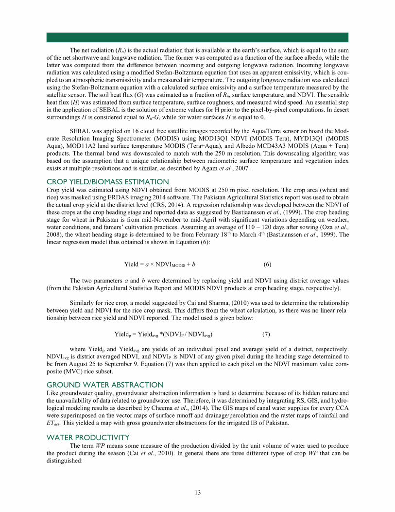
The net radiation (Rn) is the actual radiation that is available at the earth’s surface, which is equal to the sum of the net shortwave and longwave radiation. The former was computed as a function of the surface albedo, while the latter was computed from the difference between incoming and outgoing longwave radiation. Incoming longwave radiation was calculated using a modified Stefan-Boltzmann equation that uses an apparent emissivity, which is cou-pled to an atmospheric transmissivity and a measured air temperature. The outgoing longwave radiation was calculated using the Stefan-Boltzmann equation with a calculated surface emissivity and a surface temperature measured by the satellite sensor. The soil heat flux (G) was estimated as a fraction of Rn, surface temperature, and NDVI. The sensible heat flux (H) was estimated from surface temperature, surface roughness, and measured wind speed. An essential step in the application of SEBAL is the solution of extreme values for H prior to the pixel-by-pixel computations. In desert surroundings H is considered equal to Rn-G, while for water surfaces H is equal to 0.

SEBAL was applied on 16 cloud free satellite images recorded by the Aqua/Terra sensor on board the Mod-erate Resolution Imaging Spectrometer (MODIS) using MOD13Q1 NDVI (MODIS Tera), MYD13Q1 (MODIS Aqua), MOD11A2 land surface temperature MODIS (Tera+Aqua), and Albedo MCD43A3 MODIS (Aqua + Tera) products. The thermal band was downscaled to match with the 250 m resolution. This downscaling algorithm was based on the assumption that a unique relationship between radiometric surface temperature and vegetation index exists at multiple resolutions and is similar, as described by Agam et al., 2007.

CROP YIELD/BIOMASS ESTIMATION Crop yield was estimated using NDVI obtained from MODIS at 250 m pixel resolution. The crop area (wheat and rice) was masked using ERDAS imaging 2014 software. The Pakistan Agricultural Statistics report was used to obtain the actual crop yield at the district level (CRS, 2014). A regression relationship was developed between the NDVI of these crops at the crop heading stage and reported data as suggested by Bastiaanssen et al., (1999). The crop heading stage for wheat in Pakistan is from mid-November to mid-April with significant variations depending on weather, water conditions, and famers’ cultivation practices. Assuming an average of 110 – 120 days after sowing (Oza et al., 2008), the wheat heading stage is determined to be from February 18th to March 4th (Bastiaanssen et al., 1999). The linear regression model thus obtained is shown in Equation (6):

Yield = a × NDVIMODIS + b (6) The two parameters a and b were determined by replacing yield and NDVI using district average values (from the Pakistan Agricultural Statistics Report and MODIS NDVI products at crop heading stage, respectively). Similarly for rice crop, a model suggested by Cai and Sharma, (2010) was used to determine the relationship between yield and NDVI for the rice crop mask. This differs from the wheat calculation, as there was no linear rela-tionship between rice yield and NDVI reported. The model used is given below: Yieldp = Yieldavg *(NDVIP / NDVIavg) (7) where Yieldp and Yieldavg are yields of an individual pixel and average yield of a district, respectively. NDVIavg is district averaged NDVI, and NDVIP is NDVI of any given pixel during the heading stage determined to be from August 25 to September 9. Equation (7) was then applied to each pixel on the NDVI maximum value com-posite (MVC) rice subset.

GROUND WATER ABSTRACTION Like groundwater quality, groundwater abstraction information is hard to determine because of its hidden nature and the unavailability of data related to groundwater use. Therefore, it was determined by integrating RS, GIS, and hydro-logical modeling results as described by Cheema et al., (2014). The GIS maps of canal water supplies for every CCA were superimposed on the vector maps of surface runoff and drainage/percolation and the raster maps of rainfall and ETact. This yielded a map with gross groundwater abstractions for the irrigated IB of Pakistan.

WATER PRODUCTIVITY The term WP means some measure of the production divided by the unit volume of water used to produce the product during the season (Cai et al., 2010). In general there are three different types of crop WP that can be distinguished:

14


Technical WP (kg m-3) defined as the mass of product per unit of water consumed Economic WP ($ m-3) defined as net private benefits per unit of water consumed Socio-economic WP ($ m-3) defined as the net social benefits per unit of water consumed, which are difficult to

value

Depending on whether a system is food scarce, water scarce, or whether the market is completely open, one of the above crop productivities can be optimized. In simple words, technical WP is defined as the yield (kg) of crop obtained by applying a unit volume of water (m3). For agricultural systems (like in Punjab), which consist of multiple cropping patterns, WP estimations should also be made in monetary terms. The calculation of production (in physical or financial terms) and ETact leads to the determination of WP. However, assessments of the economic and socio-economic WP are beyond the scope of this work, and we have limited this study to the analysis of technical water productivities.

FIELD SURVEYS AND GROUND TRUTHING As noted above, a comprehensive field survey was carried out at representative sites to do ground truthing and verify spatial information obtained through satellites. A short, informative questionnaire was developed (See Annexure I), and the farmers were interviewed to obtain information regarding age and experience, their cropping patterns and yield of major crops (current and previous years’), source of irrigation (canal, groundwater or conjunctive), cost in-curred to irrigate their crops during the growing season, and other production costs. The soil and water quality infor-mation were also included in the survey along with GPS location information so that the soil and water quality maps developed through RS could be verified and an error matrix could be made to determine the percentage (%) error in the maps of land use, soil, and water quality. The information on irrigation mode also helped to estimate overall cost of irrigation incurred, if sources other than surface water were in use. Thus, the survey helped to calibrate and validate remote sensing information of the parameters under investigation as well as provided information on irrigation costs incurred.

RESULTS This section of the report shows the results obtained after carrying out the above detailed RS, GIS, modeling, and field surveys (in the two selected CCAs, with results then applied to all CCAs) of the irrigated IB, Pakistan.

LULC Initial clustering of five classes was applied for the separation of the total IB into (i) water/ice, (ii) barren, (iii) shrub land /grass land, (iv) natural vegetation (forests), and (v) cropland. The number of classes was then increased to iden-tify the land use. This resulted in a first round of 27 classes that provided the basis for further refinement and analysis. Classification was made by taking into consideration the cropping calendar and dominance of a particular crop in the area. The class cropland was partitioned using NDVI temporal profiles and expert knowledge of cropping patterns. Some classes were merged on the basis of information obtained during ground truthing. NDVI profile similarities were also considered during this merging. This procedure reduced the number of classes from 27 to 11. The ISODATA clustering technique run in ERDAS 2014 software’s model maker facility met the expected goal to separate phenological differences such as the start of growing season, the end of the growing season, and growing length of a particular crop. The class “irrigated rice, wheat rotation” has two distinct peaks, one at the end of February and the other at the end of August. This matches with the cropping period of wheat from November to April (i.e. Rabi) and rice from June to October (i.e. Kharif). Moreover, the area in this class was completely cultivated with only a very small percentage of fallow land. The rainfed crops have lower NDVI values and their peak timing may differ due to differences in the pattern of natural climatic conditions as compared with irrigated areas. The recession of NDVI curves for rainfed crops like “rainfed crops mixed cotton, wheat rotation/fodder” and “rainfed crops general” show similar trends as those of irri-gated crops but with lower NDVI values. The crop labeled “rainfed crops wheat/grams” shows a different trend than other rainfed crops. Under this class, only Rabi crops (wheat and grams) were grown. The resultant LULC map is presented in Figure 5.

15


Figure 5: LULC Map of the Irrigated IB Based on NDVI

The total irrigated area of Pakistan is estimated at about 16.25 mha. The dominant land use for Kharif in the irrigated IB is cotton and rice. While wheat is major Rabi crop grown in 37% of total area. Rice, cotton, and sugarcane are grown on 11%, 10%, and 3% respectively of the total irrigated area of the basin. The land use map was further investigated at selected CCAs to check the accuracy. The resulting maps for the IB for the Kharif and Rabi seasons are shown in Figure 6. Eleven land use classes were identified in the Kharif season (2008, 2010, 2013) while nine land use classes were derived for Rabi season (2008-09, 2010-11, 2013-14). In 2008, wheat was the major Rabi crop and total area under wheat in Pakistan was 8.22mha, 6.15 mha in Punjab whereas in other provinces 2.07 mha was under production. Sugarcane was sown in 1.105 mha, 0.711mha in Punjab and 0.394mha in other parts of country. Rice, a higher water use crop, was the major Kharif crop, and again Punjab is the major shareholder province where rice covered 1.845 mha, whereas other provinces only covered 0.705, and total irrigated area was 2.55mha. Cotton was grown in 2.04 mha in the Kharif season, 1.79mha in Punjab and 0.52 in other area of the country. The remaining area was covered by maize and fodder crops comprising 0.62 mha. In 2010, during the Kharif season, due to the devastating floods of 2010, land productivity was greatly re-duced, and as a result, rice was only sown in 1.84 mha area of Pakistan. Out of the 1.84 mha, 1.50 was sown in Punjab and 0.34 mha in other provinces. Similarly, a downward trend was followed by cotton which was sown in 2.01 mha. In Punjab cotton was sown on 1.60mha and 0.40 in other areas. Sugarcane covered an area 1.029 mha. Rabi shortage of canal water supply, degradation of land productivity, and late sowing decreased the wheat yield and crop coverage to 7.86 mha throughout Pakistan, with only 5.89 mha in Punjab and 1.97 mha in the rest of the country. Furthermore, maize and other crops covered 0.43mha. The LULC map of 2013-14 revealed, in Rabi season, wheat area sown rose to 9.11 mha in Pakistan, with 6.67 in Punjab and 2.44 mha in Sindh, Baluchistan, and KPK. Sugarcane was sown in 1.121 mha across the country, with 0.753 in Punjab and 0.368 in other provinces. Fodder and maize were sown in 0.81 mha in both seasons. During the Kharif season of 2013, rice was the major crop in the basin covering 2.51mha, 2.01 in Punjab and 0.5 in other areas. Cotton was sown in 2.75 mha in Pakistan, 2.3 mha in Punjab and 0.45 in other areas.

16


Figure 6: LULC Maps in the Irrigated IB for Kharif and Rabi Seasons of the Study Years (2008-09,

2010-11, and 2013-14)

17


The maps were then validated through the ground truthing survey carried out in the two selected CCAs during the Rabi season of 2013-14. A total of 136 points were collected during the ground truthing survey and used in the error matrix analysis. The farmers were interviewed and asked about their crops for the Kharif season of 2013. The goal is to take ground truthing data for each season separately, however budget constraints restricted such seasonal campaigns. Seven LULC classes were visited and have minimally three observation points. The resulting error matrix in Table 9 shows an overall accuracy of the classified map is 77.2%. Table 9: Error Matrix to Determine Overall Accuracy of the Remotely Sensed LULC Map

Class Name Omission error Commission er-

ror

Wheat 83% 80%

Sugarcane 75% 75%

Rainfed 71% 91%

Forest Area 91% 71%

Bare Soil 91% 71%

Sparse vegetation 71% 45%

Overall Accuracy 77.20%

The average error of omission (producer’s accuracy) and commission (user’s accuracy) is 80% and 75%, respectively. Hence, the overall accuracy of the land use map developed is 77.2% after the field observation. Consid-ering that the satellite resolution is coarse (6.25 hectares) and the field sizes (0.4 hectares) are small, this accuracy is rather satisfactory and in agreement with accuracy levels achieved in different land use and crop identification studies. Bastiaanssen (1998) concluded that, with extensive fieldwork, crops could be identified with an average accuracy of 86%. However, this accuracy level fluctuates from 49% to 96%, depending upon the spatial coverage of the satellites and field size.

Water Supplies and Costs Water supply is comprised of canal and groundwater with differing costs.

CANAL WATER SUPPLY Total canal water available at the farm gate for the CCAs is estimated at 77 Km3 (or 485 mm) (Figure 7).

This amount is computed from the reservoir releases and reported conveyance losses. Canal water available at farm gates varies from 200 to 900 mm yr-1. Lower Chenab canal, upper Chanab canal, and upper Dipalpur canal have 389mm, 346 mm, and 313 mm respectively. This spatial variability in canal supplies is due to the non-perennial system and variability in water released from the reservoirs. The highest rate of canal water irrigation is observed in the lower

18


Indus especially in Sindh province. Ghotki, Flueli, and Pinyari canals have 748 mm, 853 mm, and 608 mm respec-tively. The higher rate is provided in order to flush down the salinity, as these areas are suffering from salinity and a deterioration in groundwater quality (Qureshi et al., 2010) due to the high intensity of rice cultivation in this low laying river plain area. The canal water supplies are not sufficient in many CCAs to meet the crop water requirements. The deficit can only be met through groundwater irrigation. The groundwater abstraction is causing secondary salinization as a fresh layer of groundwater is being abstracted and less recharge results in abstraction of low quality groundwater.

Figure 7: GIS Maps of Canal Water Supplies for the Years 2008-09, 2010-11, and 2013-14

GROUNDWATER ABSTRACTIONS Groundwater is being extensively used to supplement limited canal water supplies especially in the CCAs

having lower WAs. The spatial groundwater map shown in Figure 8 (Cheema et al., 2014) was used as a base map to estimate the amount of groundwater abstracted during one year. The map shows gross groundwater abstraction rates for each pixel estimated by subtracting irrigation applied by canal water from total crop water use. The data shows that, on an annual basis, in most of the IB, an amount of 300 to 900 mm is being abstracted from aquifers for irrigating crops. The largest groundwater abstractions occur in the province of Punjab and the highest values for groundwater use are observed in the middle and northeastern parts of the basin. These areas contain relatively good quality ground-water resources (Arshad et al., 2007) but have lower canal WAs.

19


Figure 8: Spatial Map of Groundwater Use in the Irrigated IB

Source: Cheema et al., 2014 Note: No color implies no groundwater use in CCA or non-irrigated area or non-availability of data.

During the ground truthing in the example CCAs of LLC and MzgC, farmers were asked about their sources of irrigation to compare with the maps made above. The average groundwater abstraction in LCC is about 247mm. The MzgC CCA undergoes 180mm of groundwater abstraction annually. Higher canal WAs in the MzgC resulted in relatively less pressure on groundwater reserves as compared to LCC. About 76% and 67% of the total farmers sur-veyed in LCC and MzgC, have access to canal water (Figure 9). In the areas with high water use crops, large volumes of water are being supplied not only from canals but also from groundwater conjunctively or solely. In the LCC and MzgC command areas, 67% and 32%, respectively, of farmers were using groundwater in conjunction with canal water.

Figure 9: Sources of Irrigation in LCC and MzgC Command Area

This confirms the data presented in Figure 8 that farmers are not only relying on canal water, but that many are using canal and groundwater conjunctively.

0

25

50

75

100

Canal water Conjunctive use

Farm

er (%

age)

Source of water use

LCCMzgC

20


Irrigation Costs The dependence on groundwater has forced farmers to invest money to pump out groundwater rather than

only using canal water. This has significant implications for the costs associated with irrigation. The lowered water table has resulted in the use of deep well turbines that require more power to operate. Figure 10 shows the cost break-down for two methods of groundwater abstraction and the costs for obtaining canal water for wheat in the LCC com-mand area. This data was obtained during the ground truthing survey. The cost calculations here are as follows:

Time to irrigate one acre with 0.75 cusecs = 3.5 hours Electric motor pump = 18 (h.p)×0.746(KW)×3.5 (hr)×20 (Rs/KWH) = 940Rs/acre Diesel motor pump = 3.5(hr/acre) ×3.0(litre/hr) ×114 (Rs/litre) = 1197Rs/acre Recently fuel prices have dropped from Rs 114 to Rs 86 per litre. The recalculated cost by replacing 114 Rs/litre with 86 Rs/litre is estimated at Rs 903 / acre per irrigation. Thus, average groundwater pumping costs for wheat (Rabi crop) is Rs. 4,063 per acre when using diesel which accounts for 24.8% of total production costs in LCC according to the field survey results. However, the cost fluctuates between Rs 3,612 to Rs 4,515 depending upon number of irrigations (4 to 5 irrigations). While for rice (Kharif crop), the average pumping cost using diesel and electricity was Rs 9,030 and 8,460 per acre, respectively, in LCC. This accounts for 39% and 34% of total production cost, respectively. These high costs are compared to a flat canal water rate of Rs 50 and Rs. 85 per acre for Rabi and Kharif, respectively. Such a huge difference in cost suggests the importance of revisiting existing the WAs of the CCAs and/or the canal water rates with respect to crop water requirement. Figure 10: Cost Incurred on Irrigating One-Acre Field from Various Sources in LCC

Soil Salinity Equation 4 was used to prepare soil salinity maps for the Irrigated IB. The soil salinity maps of the irrigated IB for the years 2008-09, 2010-11, and 2013-14 are shown in Figure 11. This figure shows that soil salinity varies spatially from upper to lower IB. Salinity is lower in the upper IB, while in the middle it varies from moderate to strongly saline. However, the lower IB has the highest percentage of saline soils with the most area showing strong salinity. These spatial maps identify hot spots where soil salinity is higher. It is evident from Figure 11 that middle and lower IB have more salinity problems. According to an estimate by Basharat et al., (2014), 70% of the irrigated area of Sindh (lower Indus) is saline, thus agreeing with the estimates.

4063.5

9030

3807

8460

50 850

2000

4000

6000

8000

10000

12000

Rabi Kharif Rabi Kharif Rabi Kharif

Diesel Electric Canal

Cost

(R

s/ a

cre)

21


Figure 11: Spatial Maps of Soil Salinity in the Entire Irrigated IB during the Study Years

The area wise changes in million ha with different levels of soil salinity is shown in Figure 12. Figure 12 shows soil salinity status in the irrigated IB for the years 2008-09, 2010-11, and 2013-14. The estimates show that in year 2008-09, 10.18, 4.41, and 1.65 mha area are categorized as non-saline, moderate, and strongly saline, respec-tively. While in 2010-11, 9.14, 4.86, and 2.24 mha are detected as non-saline, moderate, and strongly saline areas, respectively. However, in 2013-14, 8.36 mha is under non-saline, and 4.79 mha and 3.09 mha are under moderate and strongly saline areas.

Figure 12: Temporal Change in Soil Salinity in the Irrigated IB

The overall percent decrease in non-saline area from year 2008-09 to 2013-14 is 11%, as it decreases from 62.5% to 51.5% during the time span of five years. While, in the case of moderate and strongly saline soils, the percent area increase is estimated at 9% and 2.5%, respectively. The soil quality was further investigated at the canal command level. Some canal commands have salinity at more profound levels than others. It increases going from the upper to lower basin. The estimates shows that lower Chenab canal, Upper Chenab canal, upper Jhelum canal, and lower Jhelum canal are 66%, 63%, 73.5%, and 72% non-

0

2

4

6

8

10

12

2008 2010 2013

Are

a (

mh

a)

Non Saline Moderate Saline Strongly Saline

22


saline, respectively. Salinity increases lower in the basin as Begari, Flueli, Pinyari, and Nara canals have 27%, 18.4%, 23.6%, and 29% of their area classified as strongly saline, respectively.

The ground measurements of soil salinity obtained during field surveys conducted in the representative CCAs of LCC and MzgC were used to check the accuracy of the salinity maps by comparing the results with pixel-based estimates. A reasonable correlation was found between observed (SSIn-situ) and remote sensing estimated (SSRS) soil salinity with a coefficient of determination (R2) of 0.65 and Pearson’s r estimated at 0.81 as shown in Figure 13 for 141 ground measurements.

Figure 13: Comparison SSRS and SSIn-situ Soil Salinity from 141 Ground Measurements

Groundwater Quality As described above, the hidden nature of groundwater hampers developing spatial maps through remote sensing. Therefore, an indirect method was adopted to estimate groundwater quality. Regression models were developed based on electrical conductivity using in-situ water quality (ECGW) measured at 80 locations and spatial soil quality (ECsoil ) data (pixel values) with R2 and Pearson’s r estimated at 0.73 and 0.86, respectively as shown in Figure 14.

y = 1.2747xR² = 0.65n= 141

0.0

1.0

2.0

3.0

4.0

5.0

0.0 1.0 2.0 3.0 4.0 5.0

SSIn

-situ

(dS

m-1

)

SSRS (dS m-1)

23


Figure 14: Comparison between ECsoil and ECGW Measured at 80 Locations of the Irrigated IB

The regression model shown in Figure 14 was used to develop spatially distributed groundwater quality maps for the IB shown in Figure 15.

Figure 15: Water Quality Map of Irrigated IB Developed Using Interpolation of Point Data

y = 0.5325xR² = 0.73

Pearson's r = 0.86n = 80

0.00

2.00

4.00

6.00

8.00

0.00 2.00 4.00 6.00 8.00

ECgw

ECsoil

24


Figure 15 shows spatial change in groundwater quality within the irrigated IB. Water quality is an issue in the middle and lower IB with some tracts of fresh water. Canals in the upper IB like Lower Chenab canal, Upper Chenab canal, and Mailsi canals have groundwater well fit for irrigation, while canals in the middle of the basin like Abbasia and MzgC have relatively marginal water quality, and canal commands areas in lower part of the basin like Begari, Nara, and pinyari have unfit groundwater quality. Northern parts of the basin receive the highest rainfall thus helping recharge groundwater aquifers. Therefore, the quality of ground water is relatively better in the upper IB.

Crop Water Use ETact or actual water used by the crop, was estimated using SEBAL for the years 2008-09, 2010-11, and 2013-14 as given in Figure 16. ETact values change from upper to lower parts of the basin. Figure 16: Spatially Distributed Annual ETact Values Estimated for the Irrigated IB for the Years

Spatial maps of ETact helped to discern crop water use for each CCA of the basin. Total annual ETact for the year 2013 in LCC and MzgC command areas was estimated at 1,023 mm and 928 mm, respectively. Comparatively, in the lower IB, Pinyari and Flueli CCAs had 871mm and 933 mm per year, respectively. Figures 17 and 18 show the ETact for various CCAs during the Rabi and Kharif seasons, respectively.

25


Figure 17: ETact Estimated for Various CCAs in the Irrigated IB for the Rabi Season 2013-14

Figure 18: ETact Estimated for Various CCAs in the Irrigated IB for the Kharif Season 2013-14

The average ETact for Rabi and Kharif season was estimated at 353 mm and 532 mm, respectively. During Rabi season, high values of ET were observed in LBDC, Pakpattan, and Sidhnai canals showing 492 mm, 478 mm, and 462 mm, while average values of ET in LCC, Haveli, Pat Feeder, and Flulei canals were 425, 412, 386, and 357 mm, respectively. However, Sadiqia, Bannu, and Abbsasia are low yield areas, and as result, their values are very low; showing 230, 211, and 207, respectively. During the Kharif season, more than 600 mm of water were used by crops in 14 CCAs. Among these canal commands, Pat Feeder had the highest canal water use at 796 mm. Beghari, North-west, and Rice canals are also in similar range with 795 mm, 793 mm, and 789 mm, respectively. The crop water use in LCC was 425 mm in Rabi season and was 428mm in MzgC command. While in Kharif, the estimated use in LCC was 598mm as compared to MzgC command with 500 mm of water used. In the lower IB, crop water use for Pinyari and Flueli canal commands were 345 and 357 mm in Rabi and 526 and 576 mm during Kharif, respectively. Thal,

0

100

200

300

400

500

Ban

nu Thal

UJC LJC

CR

BC

Mar

ala

Rav

iU

CL

LCC

Ray

a B

ranc

hC

BD

CLB

DC

Ran

gpur

UD

CH

avel

iLD

CM

ZGSi

dhna

iPa

kpat

tan

DG

Ford

wah

Sadi

qia

U. B

ahaw

al &

Qai

mB

ahaw

alA

bbas

iaPa

njna

dPa

t fee

der

Des

ert

Beg

ari

Gho

tki

Nor

th W

est

Ric

eK

hairp

ur W

est

Dad

uK

hairp

ur (E

)R

ohri

(N)

Roh

ri (S

)Li

ned

Nar

aFu

leli

Piny

ari

Gaj

a B

ranc

hK

alri

ETac

tR

abi s

easo

n (m

m)

CCAs

0100200300400500600700800

Ban

nu Thal

UJC LJC

CR

BC

Mar

ala

Rav

iU

CL

LCC

Ray

a B

ranc

hC

BD

CLB

DC

Ran

gpur

UD

CH

avel

iLD

CM

ZGSi

dhna

iPa

kpat

tan

DG

Ford

wah

Sadi

qia

U. B

ahaw

al &

Qai

mB

ahaw

alA

bbas

iaPa

njna

dPa

t fee

der

Des

ert

Beg

ari

Gho

tki

Nor

th W

est

Ric

eK

hairp

ur W

est

Dad

uK

hairp

ur (E

)R

ohri

(N)

Roh

ri (S

)Li

ned

Nar

aFu

leli

Piny

ari

Gaj

a B

ranc

hK

alriET

act

Kha

rif se

ason

(mm

)

CCAs

26


Bannu, and CRBC canals are lower water use canals, but their values were more in the Rabi season consisting of 233 mm for Bannu, 420mm for Thal, and 318mm for CRBC.

Crop Biomass/Yield The crop yield map of the two major staple crops (wheat and rice) grown in the irrigated IB is shown in Figure 19. The spatial map was produced using land use and biomass information of rice and wheat for the year 2013-14 using ERDAS Imagine 2014. Figure 19: Yield Map of Wheat & Rice Crops Extracted from Biomass Information for the Year

2013-14

The accuracy of the developed map was validated using district production data retrieved from the Agricul-

tural Statistics of Pakistan. A comparison was made between fractional yield (tonnes/ha in a district) obtained from the agricultural statistics and estimated by remote sensing. The validation (Figure 20) shows a reasonable agreement between estimated and actual district level data with an R2 of 0.64 and a Pearson’s r estimated at 0.80 for wheat crop. While for rice crop, the R2 and Pearson’s r are estimated at 0.54 and 0.73, respectively.

27


Figure 20: Comparison between Yield Fraction RS and Yield Fraction Reported for Wheat and Rice

Yield Fraction w.r.t Area

Wheat, being the major Rabi crop, was sown in large tracts of the IB, however, its yield varies in different CCAs. The variation in wheat yields ranged from 5,280 to 700 kg ha-1, while rice yields varied from 3,300 to 1,900 kg ha-1. Figures 21 and 22 show the yields of wheat and rice, respectively, in the various CCAs of the IB during 2013-14.

Figure 21: Wheat Yield in CCAs of the IBIS in 2013-14

y = 0.8621x + 0.831R² = 0.64

0.0

1.0

2.0

3.0

4.0

5.0

0.0 1.0 2.0 3.0 4.0 5.0Whe

at y

ield

frac

tion r

epor

ted

(tonn

es h

a-1)

Wheat yield fractionRS (tonnes ha-1)

y = 0.524x + 0.6973R² = 0.54

0.0

1.0

2.0

3.0

4.0

0.0 1.0 2.0 3.0 4.0

Ric

e yi

eld

frac

tion r

epor

ted

(tonn

es h

a-1)

Rice yield fractionRS (tonnes ha-1)

0

1000

2000

3000

4000

5000

Ban

nu Thal

UJC LJC

CR

BC

Mar

ala

Rav

iU

CL

LCC

Ray

a B

ranc

hC

BD

CLB

DC

Ran

gpur

UD

CH

avel

iLD

CM

ZGSi

dhna

iPa

kpat

tan

DG

Ford

wah

Sadi

qia

U. B

ahaw

al &

Qai

mB

ahaw

alA

bbas

iaPa

njna

dPa

t fee

der

Des

ert

Beg

ari

Gho

tki

Nor

th W

est

Ric

eK

hairp

ur W

est

Dad

uK

hairp

ur (E

)R

ohri

(N)

Roh

ri (S

)Li

ned

Nar

aFu

leli

Piny

ari

Gaj

a B

ranc

hK

alri

Whe

at y

ield

(Kg

ha-1

)

CCAs

28


Figure 22: Rice Yield in CCAs of the Irrigated IB in 2013-14

The highest yields of wheat were observed in the lower and upper Jhelum CCAs at 5,280 kg ha-1 and 5,070 kg ha-1, respectively. Similar results are also seen in Lower Bari Doab Canal (LBDC) and Rohri South Canal producing 3918 kg ha-1 and 3714 kg ha-1. Wheat yields in LCC and MzgC were 3,486 and 2,685 kg ha-1 respectively, which are renowned for wheat/rice-cotton rotation and producing smaller yield as compared to reported trends. Similarly, lower yields are also shown in Desert and DG canals producing 1890 kg ha-1 and 1206 kg ha-1 respectively. The variation in yields of wheat is not only due to variation in management practices but also due to soil and water quality. Pinyari and Flueli CCAs are examples of such canals where soil and water conditions are worse; they were producing 1,710 kg ha-1 and 1,740 kg ha-1. Lower wheat yield may partly be attributed to the unfavorable weather conditions and partly to the later sowing of the crop than recommended. Moreover, more rain in the month of February and April causes disease in wheat crop. Thus, unfavorable weather conditions may be responsible for lower than normal yield. In the case of rice, yields in LCC, MzgC, Pinyari, and Fleuli CCAs were estimated at 2,652, 3,310, 3,185, and 3,297 kg ha-

1, respectively. Forwadh and Saddiqua, however, are low rice producing canals, and their values were 2,388 kg ha-1

and 1,925 kg ha-1.

Water Productivity Calculating technical WP from the RS and GIS analysis is one of the final objectives of the project. Technical WP gives kilograms of yield produced per unit volume of water used, as described earlier. Using the crop yield and ETact provided above, spatially distributed WP maps can be produced. The maps of WP for wheat and rice crops are provided in Figure 23. They show that wheat areas with higher WP lie in the middle part of the basin. When compared with the earlier map of canal water supplies (Figure 7), this is especially true in CCAs with lower WA. One reason for this higher WP is the use of groundwater in areas where sufficient surface water is not available.

0

500

1000

1500

2000

2500

3000

3500

Ban

nu Thal

UJC LJC

CR

BC

Mar

ala

Rav

iU

CL

LCC

Ray

a B

ranc

hC

BD

CLB

DC

Ran

gpur

UD

CH

avel

iLD

CM

ZGSi

dhna

iPa

kpat

tan

DG

Ford

wah

Sadi

qia

U. B

ahaw

al &

Qai

mB

ahaw

alA

bbas

iaPa

njna

dPa

t fee

der

Des

ert

Beg

ari

Gho

tki

Nor

th W

est

Ric

eK

hairp

ur W

est

Dad

uK

hairp

ur (E

)R

ohri

(N)

Roh

ri (S

)Li

ned

Nar

aFu

leli

Piny

ari

Gaj

a B

ranc

hK

alri

Ric

e yi

eld

(Kg

ha-1

)

CCAs

29


Figure 23: WP Map of Wheat and Rice Crops in the Irrigated IB

The CCA WP information for wheat is graphed in Figure 24. It shows that WP of wheat is variable with a maximum WP of 1.34 kg m-3 and a minimum WP estimated at less than 0.2 kg m-3. The mean, median, and standard deviation are estimated at 0.66, 0.59, and 0.31 kg m-3, respectively. The LJC CCA has the highest WP of 1.34 kg m-3. Furthermore, Upper Chenab Canal (UJC), Dipalpur, and CBD canals were high water productivity canals. However, our ground truthing showed that in some canals proper management techniques were not followed and farmers did not know when and how much water was applied. Poor water/soil quality was also among major causes of low water productivity. Rice, Beghari, North-West and Dadu, were among these canals, and their values were less than 0.30 kg m-3. Wheat WP of various CCAs certainly shows some variation as LCC and MzgC CCAs have 0.82 and 0.63 kg m-

3, respectively, while in Pinyari and Flueli, WP is estimated at 0.50 and 0.49 kg m-3, respectively. Figure 24: Wheat WP (kg m-3) in Different CCAs of the Irrigated IB

Similarly the WP of rice is provided in Figure 25. The maximum and minimum WP is estimated at 1.12 kg m-3 and 0.34 kg m-3, respectively with mean, median, and standard deviation estimated at 0.59 kg m-3, 0.57 kg m-3,

0.00

0.20

0.40

0.60

0.80

1.00

1.20

Ban

nu Thal

UJC LJC

CR

BC

Mar

ala

Rav

iU

CL

LCC

Ray

a B

ranc

hC

BD

CLB

DC

Ran

gpur

UD

CH

avel

iLD

CM

ZGSi

dhna

iPa

kpat

tan

DG

Ford

wah

Sadi

qia

U. B

ahaw

al &

Qai

mB

ahaw

alA

bbas

iaPa

njna

dPa

t fee

der

Des

ert

Beg

ari

Gho

tki

Nor

th W

est

Ric

eK

hairp

ur W

est

Dad

uK

hairp

ur (E

)R

ohri

(N)

Roh

ri (S

)Li

ned

Nar

aFu

leli

Piny

ari

Gaj

a B

ranc

hK

alriWat

er P

rodu

ctiv

ity (k

g m

-3)

CCAs

30


and 0.17 kg m-3. The highest WPs are found in Upper Dipalpur, CRBC, Khairpur east, and Rangpur canals showing 1.12 kg m-3, 0.90 kg m-3, 0.82 kg m-3, and 0.79 kg m-3. The WPs of LCC, MzgC, Pinyari, and Flueli CCAs are estimated at 0.44, 0.66, 0.61 and 0.57 kg m-3, respectively. However, as in case of wheat, Beghari, Desert, Pat feeder, and Rice showed lower rice WP of 0.34 kg m-3, 0.34 kg m-3, 0.36 kg m-3, and 0.37 kg m-3.

Figure 25: Rice WP (kg m-3) in Various CCAs of the Irrigated IB

The WP estimated in this study is in agreement with some of previous studies performed in the region. Cai and Sharma (2010) estimated average rice WP for the Indo-Gangetic plain at 0.74 kg m-3. The minimum and maximum WP and standard deviation were estimated at 0.18, 1.8, and 0.32 kg m-3, respectively. Ahmad et al., (2004) estimated an average WP in rice-wheat cropping zones of Punjab province that ranged between 0.4 to 1.6 kg m-3. Water Watch in 2003 estimated a 0.45 kg m-3 average WP for rice crops in the IB (Waterwatch, 2003).

DISCUSSION OF RESULTS

This section concludes the paper with a discussion based on the results presented above and what analysis can be teased out from comparisons between them. Information presented on WA, water delivered in a particular year, crop water use, groundwater use, yields, and WP for each canal command provides an insight to revisit WA rules. The comparison of these parameters for each canal command is given in Table 10. Water allocation varies (in the whole sample) from 2.5 to 16 cusec per 1,000 acres (i.e. 0.18 – 1.15 litre/sec/hectare). Rice, Beghari, Pinyari, Flueli, Marala Ravi, and Gaja branch canal commands have higher WA (> 10 cusec/1000 acres) and most of these CCAs are in the lower IB. While Thal, Upper Jhelum, Lower Jhelum, LCC, Northwest, Khairpur East, Saddiquia, and Lower Bari Doab Canal commands have lower WA (<5 cusec / 1,000 acres). However, Mzg and DG Canals’ WA are 8.2 and 8.6 cusec /1000 acres, respectively. Most of these canal commands lie in middle of the IB. Water diverted at the canal head for the above mentioned CCAs is higher in the case of Rice and Flueli canals, where the depth of water diverted was 2,102 and 1,220 mm, respectively. Pinyari and Beghari receive 869 and 832 mm, but water delivered in the case of Marala Ravi and Gaja branch canals is merely 382 and 402 mm, respectively. Similarly, among canals with lower WA, Upper Jhelum and Saddiquia received 1,031 and 861 mm, respectively, while Northwest, Lower Bari Doab, Khairpur East, LCC, Thal, and Lower Jhelum canals received 763, 724, 618, 556, 516, and 452 mm, respectively thus showing anomalies in WA and delivered quantity as well. However, water diver-sions at the heads of Mzg and DG canals are 1,260 and 1,097mm, respectively.

00.20.40.60.8

11.2

Ban

nu Thal

UJC LJC

CR

BC

Mar

ala

Rav

iU

CL

LCC

Ray

a B

ranc

hC

BD

CLB

DC

Ran

gpur

UD

CH

avel

iLD

CM

ZGSi

dhna

iPa

kpat

tan

DG

Ford

wah

Sadi

qia

U. B

ahaw

al &

Qai

mB

ahaw

alA

bbas

iaPa

njna

dPa

t fee

der

Des

ert

Beg

ari

Gho

tki

Nor

th W

est

Ric

eK

hairp

ur W

est

Dad

uK

hairp

ur (E

)R

ohri

(N)

Roh

ri (S

)Li

ned

Nar

aFu

leli

Piny

ari

Gaj

a B

ranc

hK

alri

Wat

er P

rodu

ctiv

ity (k

g m

-3)

CCAs

31


Table 10: Satellite Based ETact, Groundwater Use, Yield and Water Productivity for Each Canal

Command in the Irrigated IB

Kharif Rabi Wheat Rice Wheat Rice

Cusec (mm) (km3) (mm) (mm) (mm) (kgha-1) (kgha-1) (kgm-3) (kgm-3) (%)

Bannu 3.3 - - - 233 211 - - - 9.1

Upper Swat 2.7 - - - - - - - - - -

Lower Swat 2.2 - - - - - - - - - -

Kabul River 2.3 - - - - - - - - - -

Warsak (L) 2.1 - - - - - - - - - -

Warsak (R) 3.2 - - - - - - - - - -

PHLC 9.8 - - - - - - - - - -

Thal 2.2 516 5.6 55 420 236 1950 2957 0.83 0.7 21.6

UJC 2.9 1031 2.7 73 701 419 5070 2920 1.21 0.42 5.3

LJC 3 452 3.2 171 501 395 5280 3180 1.34 0.63 3.4

CRBC 22.6 521 0.5 108 318 269 3111 2869 1.16 0.9 11.3

Marala Ravi 12.3 385 0.3 276 577 389 2022 2712 0.52 0.47 2.4

UCL 5.3 496 2.1 239 597 391 1962 2667 0.5 0.45 13.6

LCC 3.2 556 0.8 247 598 425 3486 2652 0.82 0.44 13.4

Raya Branch 7 346 0.6 207 512 352 1152 2551 0.33 0.5 3.3

CBDC 9 533 1.7 140 488 380 3930 2980 1.03 0.61 5.8

LBDC 4.3 724 5.5 297 644 492 3918 3026 0.8 0.47 9.5

Rangpur 6.9 670 1.1 94 328 259 1395 2586 0.54 0.79 24.8

UDC 5 447 0.8 186 264.5 427 5022 2965 1.18 1.12 6.9

Haveli 13.7 597 0.4 172 565 412 3966 3196 0.96 0.57 28.2

LDC 6.5 637 0.3 - 637 475 3120 - 0.66 - 3.9

MZG 8.2 1260 4.1 179 500 428 2685 3310 0.63 0.66 9.8

Sidhnai 5.3 707 2.4 285 626 462 2493 3254 0.54 0.52 8.5

Pakpattan 5.9 620 2.6 285 622 478 3810 3028 0.8 0.49 6

DG 8.6 1097 4.3 126 466 264 1206 3169 0.46 0.68 13.4

Fordwah 6.4 546 1.2 242 481 343 1443 2388 0.42 0.5 7.4

Sadiqia 4.3 861 4 170 290 230 840 1925 0.37 0.66 9.2

U.Bahawal & Qaim 27 700 0.3 37 361 256 1320 2738 0.52 0.76 5.3

Bahawal 6.9 818 2.7 167 422 250 930 2925 0.37 0.69 6.7

Abbasia 6.9 475 0.3 211 426 207 1737 3312 0.84 0.78 10.2

Panjnad 6.1 794 5 306 651 338 2049 3069 0.61 0.47 8.5

Pat feeder 7.1 571 1.9 241 796 386 - 2840 - 0.36 10.6

Desert 28 1155 1.9 552 743 376 1890 2563 0.5 0.34 27.1

Begari 13.6 832 3.5 373 795 424 630 2733 0.15 0.34 27.1

Ghotki 8.1 1069 4.2 211 473 232 1182 2890 0.51 0.61 10.2

North West 4.2 763 3.5 269 793 433 702 2922 0.16 0.37 19.5

Rice 16.8 2102 4.7 215 789 427 423 2901 0.1 0.37 11.5

Khairpur West 5.2 790 1.9 274 607 376 3915 2684 1.04 0.44 6.6

Dadu 5.1 794 1.9 276 474 315 798 2880 0.25 0.61 28.4

Khairpur East 4.2 618 1.8 123 321 194 1983 2639 1.02 0.82 25.1

Rohri (North) 9 531 2.5 279 600 396 2913 2738 0.74 0.46 11.1

Rohri (South) - 544 3.4 210 538 399 3714 2934 0.93 0.52 21.4

Lined - 546 1.1 - 454 314 1683 3184 0.54 0.7 22.1

Nara 5 910 9.1 196 385 267 1560 2903 0.58 0.75 28.9

Fuleli 12.4 1220 5.1 156 576 357 1740 3297 0.49 0.57 18.4

Pinyari 13.5 869 3.5 285 526 345 1710 3185 0.5 0.61 23.6

Gaja Branch 11 402 0.2 172 604 414 3519 3115 0.85 0.52 -

Kalri 8 858 0.5 114 412 322 2070 3031 0.64 0.74 31.8

ETact Yield WP Saline

Area

GW

UseWater DeliveredWA Canal

Commands

32


The annual water use by crops in the six canals with the highest WAs varies from 871 to 1,219 mm, while in the eight lowest WA canals it ranges between 426 to 1,226 mm per year. The annual water use by crops in LCC, MzgC, Fluleli, and Pinyari are 1,023, 928, 933 and 871 mm, respectively. Since wheat and rice are the major crops grown in the basin during Rabi and Kharif, WP analysis was per-formed for these two crops. The rice yield is 2,652 Kg ha-1 and 3,310 Kg ha-1 in the example CCAs of LCC and MzgC, respectively. WP of rice and wheat in LCC is 0.44 and 0.82, respectively. In MzgC, WP of rice and wheat is 0.66 kgm-

3 and 0.63 kg m-3, respectively. This depicts that LCC has a higher WP in the case of wheat, even though water availability is less than what is required. Farmers thus have to pump groundwater more to supplement surface supplies resulting in increased costs. The rice WP is lower in LCC which demands a revisit of the cropping system, as irrigation through groundwater is not only increasing costs but also shows lower productivities. Initially, these variations were based on cropping intensity, soil salinity, as well as groundwater use. But, as we have discussed, the variation in water allocations affected the crop yields and increased use of groundwater. The WP increased in CCAs having low WA with the use of groundwater, but excessive groundwater pumpage can ad-versely affect the soil and water quality as well as cause higher investments costs. The reduced surface supplies and use of poor groundwater quality can also result in lowered crop yields. Low WP, especially in CCAs receiving higher WAs, is a point of concern. A decreasing trend is found between WP and WA, shown in Figure 26. Such a trend depicts that CCAs receiving higher WAs are prone to lower WP. Average crop water use is variable for different CCAs, and crop yield also varies, thus affecting overall WP.

Figure 26: Relationship between WA (cusec) and Wheat WP (kg m-3) in CCAs of IBIS

Moreover, the CCAs receiving more water are also more prone to water logging, while the opposite is true for groundwater abstraction; CCAs where excessive groundwater abstraction is being carried out are prone to second-ary salinization. The area under salinity has shown an increasing trend during last five years, as the acreage that is strongly saline has increased by 2.5% from 2008 to 2013. This increase in salinity level in the CCAs can be linked with a decrease in the WP level (Figure 27).

y = 1.0234e-0.086xR² = 0.246

n = 43

0.00

0.40

0.80

1.20

1.60

0.0 4.0 8.0 12.0 16.0 20.0

Wat

er p

rodu

ctiv

ity (

kg m

-3)

Water allowance (cusec)

33


Figure 27: Relationship between Soil Salinity and Wheat WP (kg m-3) in the IBIS

Based on the above, it seems possible to rationalize water allocations so that each farmer in the system can access and use water efficiently while reducing costs associated with groundwater pumpage. As the study has focused on the physical and technical aspects of water use and productivity, the economics of water pricing are beyond the scope of implications that can be fully drawn. Nonetheless, we present three illustrative approaches to how the infor-mation generated in the analysis using RS and GIS mapping might inform policy decisions. Further study will be needed to investigate the economy of water allocation and water pricing, but beginning with a firm understanding of the physical variables, and how they might interact with price, is important. The current canal water pricing system based on a flat rate cannot be considered as an equity-based solution. In monetary terms, it is suggested to change the current water pricing system to a more justifiable water pricing system that should be based on amount of water used. Three different solutions, from simple to complex, based on revised water pricing or allocation rules, are illustrated below. These could be implemented to replace the current water pric-ing/allocation system.

1. Incremental WA based water pricing 2. Variable WP-WA based pricing 3. Variable WP-salinity based allocation

Incremental WA Based Water Pricing The simplest form of water pricing would be an incremental WA based system. This includes an increase in cost, i.e. rupees (Rs) per cusec, of water allocated per 1,000 acres. The base price for one to three cusec of WA is set at the current rates of Rs 50 (Rabi) and Rs. 85 (Kharif), while each additional cusec pays a 40% increase on the previous rate. The rate for WA in fractions of integer values can be determined using the unity (mathematical) method. Table 11 shows the incremental pricing structure for increasing WAs. Table 11: Incremental Pricing Rule Based on Incremental WA

Slab.No WA (cusec per 1000

acres)

Water price (Rs)

Rabi Kharif

1 1-3 50 85 2 4 70 119 3 5 98 167 4 6 137 233 5 7 192 327 6 8 269 457 7 9 376 640 8 10 527 896 9 >10 738 1,254

y = -12.91ln(x) + 10.125R² = 0.33

0

10

20

30

40

50

60

0.00 0.50 1.00 1.50

Salin

ity (%

age)

Water productivity (kg m-3)

34


Based on this incremental pricing rule, canal water cost for each CCA is calculated and provided in Figure 28 (as an example) assuming there is no adjustment in water allocations. The CCAs having high WA (> 10 cusec) have to pay 738 Rs for the entire Rabi season and 1,254 Rs for the Kharif season. Presumably, the pricing differentials would then lead to reallocation, with less water going to CCAs currently having the highest allocations and more water to those currently with lower allocations. Even the highest surface water price in this example it is still lower than the cost of groundwater pumpage, the pricing scheme could help rationalize water costs and usage.

Figure 28: Water Price for Rabi Season in Various CCAs of the IBIS

Variable Water Productivity Based Pricing The second possibility put forth for canal water pricing is based on WA by considering WP in specific CCAs. The CCAs receiving higher WAs have lower WP as shown in Figure 26 for wheat. Therefore, it might be useful to have a water-pricing system that not only considers WA but also WP. An illustration of this system of water pricing is provided below (Table 12) for the Rabi season using an increase in cost based on the WA and an adjustment based on WP for wheat. This example could be expanded to other crops using the respective WA and WP. For Rabi, the lowest water price is Rs 20 when allowance is 1 cusec per 1,000 acres and water productivity is greater than 1.0. Price increases by a fixed rate of Rs 20 for each allowance increase of 1 cusec/1,000 acres. Simultaneously, if WP drops to between 0.99 to 0.80 kg m-3, then the cost will be increased by 25% from the higher WP and likewise for further reductions in WP. Table 12 shows the matrix of pricing results. In this illustration, total price of water is calculated with the maximum amount payable under this rule of Rs 671. Table 12: Incremental Water Pricing Based on WP and Allowance for Wheat

0

200

400

600

800

Ban

nuTh

alU

JC LJC

CR

BC

Mar

ala

Rav

iU

CL

LCC

Ray

a B

ranc

hC

BD

CLB

DC

Ran

gpur

UD

CH

avel

iLD

CM

ZGSi

dhna

iPa

kpat

tan

DG

Ford

wah

Sadi

qia

U.B

ahaw

al &

…B

ahaw

alA

bbas

iaPa

njna

dPa

t fee

der

Des

ert

Beg

ari

Gho

tki

Nor

th W

est

Ric

eK

hairp

ur(W

)D

adu

Kha

irpur

(E)

Roh

ri (N

)R

ohri

(S)

Line

dN

ara

Fule

liPi

nyar

iG

aja

Bra

nch

Kal

ri

Wat

er p

rice

(Rs)

Canal command area

1 2 3 4 5 6 7 8 9 10 >10

>1.0 20 40 60 80 100 120 140 160 180 200 2200.8 0.99 25 50 75 100 125 150 175 200 225 250 2750.6 0.79 31 63 94 125 156 188 219 250 281 313 3440.4 0.59 39 78 117 156 195 234 273 313 352 391 4300.2 0.39 49 98 146 195 244 293 342 391 439 488 537

<0.2 61 122 183 244 305 366 427 488 549 610 671

Rate (Rs)

Water Productivity(kg

m-3)

Water allowance (cusec)

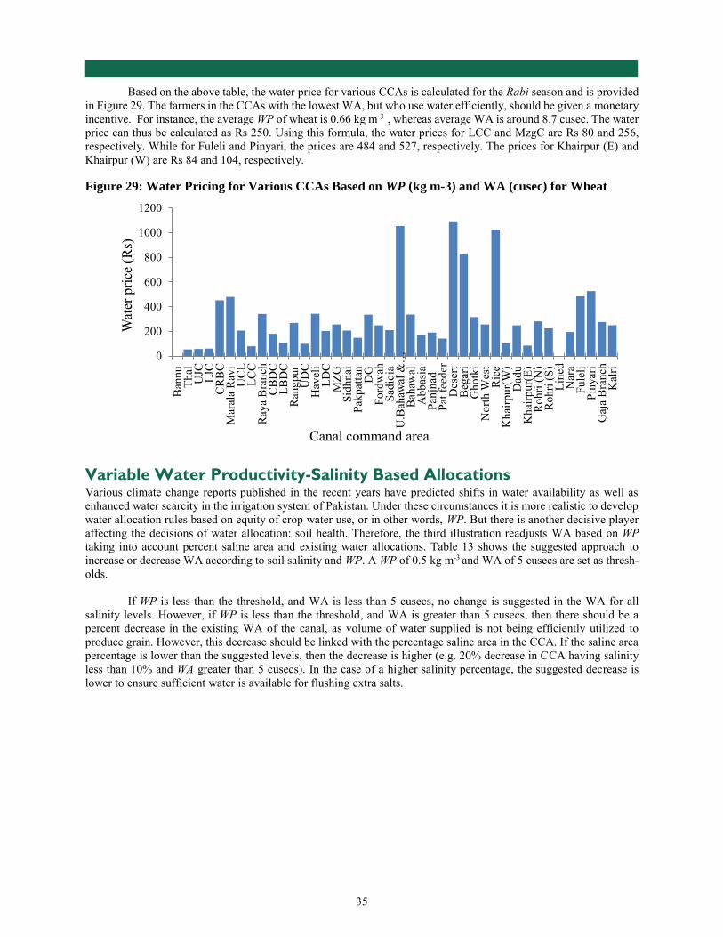
35


Based on the above table, the water price for various CCAs is calculated for the Rabi season and is provided in Figure 29. The farmers in the CCAs with the lowest WA, but who use water efficiently, should be given a monetary incentive. For instance, the average WP of wheat is 0.66 kg m-3 , whereas average WA is around 8.7 cusec. The water price can thus be calculated as Rs 250. Using this formula, the water prices for LCC and MzgC are Rs 80 and 256, respectively. While for Fuleli and Pinyari, the prices are 484 and 527, respectively. The prices for Khairpur (E) and Khairpur (W) are Rs 84 and 104, respectively.

Figure 29: Water Pricing for Various CCAs Based on WP (kg m-3) and WA (cusec) for Wheat

Variable Water Productivity-Salinity Based Allocations Various climate change reports published in the recent years have predicted shifts in water availability as well as enhanced water scarcity in the irrigation system of Pakistan. Under these circumstances it is more realistic to develop water allocation rules based on equity of crop water use, or in other words, WP. But there is another decisive player affecting the decisions of water allocation: soil health. Therefore, the third illustration readjusts WA based on WP taking into account percent saline area and existing water allocations. Table 13 shows the suggested approach to increase or decrease WA according to soil salinity and WP. A WP of 0.5 kg m-3 and WA of 5 cusecs are set as thresh-olds. If WP is less than the threshold, and WA is less than 5 cusecs, no change is suggested in the WA for all salinity levels. However, if WP is less than the threshold, and WA is greater than 5 cusecs, then there should be a percent decrease in the existing WA of the canal, as volume of water supplied is not being efficiently utilized to produce grain. However, this decrease should be linked with the percentage saline area in the CCA. If the saline area percentage is lower than the suggested levels, then the decrease is higher (e.g. 20% decrease in CCA having salinity less than 10% and WA greater than 5 cusecs). In the case of a higher salinity percentage, the suggested decrease is lower to ensure sufficient water is available for flushing extra salts.

0

200

400

600

800

1000

1200

Ban

nuTh

alU

JC LJC

CR

BC

Mar

ala

Rav

iU

CL

LCC

Ray

a B

ranc

hC

BD

CLB

DC

Ran

gpur

UD

CH

avel

iLD

CM

ZGSi

dhna

iPa

kpat

tan

DG

Ford

wah

Sadi

qia

U.B

ahaw

al &

…B

ahaw

alA

bbas

iaPa

njna

dPa

t fee

der

Des

ert

Beg

ari

Gho

tki

Nor

th W

est

Ric

eK

hairp

ur(W

)D

adu

Kha

irpur

(E)

Roh

ri (N

)R

ohri

(S)

Line

dN

ara

Fule

liPi

nyar

iG

aja

Bra

nch

Kal

ri

Wat

er p

rice

(Rs)

Canal command area

36


Table 13: WA Change Based on Areal Soil Salinity (%) and WP

Saline area (%)

Water Productivity (Kg m-3)

WA (cusec/1000 acres) Percent Change in

WA

0 – 10

<0.5 <5 No Change >5 20%(D) > 0.5 <5 10%(I) >5 No Change

11 – 20

<0.5 <5 No Change >5 15%(D) >0.5 <5 10%(I) >5 No Change

21 – 30

<0.5 <5 No Change >5 10% (D) >0.5 <5 15%(I) >5 No Change

>30

<0.5

<5 No Change >5 07%(D)

>0.5 <5 20%(I)

>5 No Change Note: D is “decrease” and I stand for “increase”.

Summary and Areas for Further Study In this study, a comprehensive spatial knowledge base on various hydrological parameters using satellite imagery, GIS, and modeling was prepared. The database on canal WAs and diversions, LULC, soil and water quality, ground water use, crop water use (or ETact), crop yield, and WP were used to analyze the current irrigation system, its efficacy, and performance. Based on performance of water use, a revisit of available water allocations was carried out and water pricing mechanisms suggested, as the current canal water pricing system based on a flat rate shouldn’t be considered as an equity-based solution. The combination of ET and crop yields determines WP of wheat and rice (the major crops of Rabi and Kharif season). The WP in combination with the spatial information on soil salinity and groundwater quality provided an opportunity to suggest water pricing rules with complex conjunctive use patterns. Three different solutions, from simple to complex, based on revised water pricing or allocation rules were suggested that could be implemented to replace the current water pricing/allocation system including 1) Incremental WA based water pricing; 2) Variable WP-WA based pricing and 3) Variable WP-salinity based allocation. It is as-sumed that the suggested water pricing mechanism will provide an opportunity to identify well performing CCAs as well as monitor the productivity of each canal command. In moving this avenue of research forward from the ideas presented, another rule that could be adopted is based on near real time monitoring of the crop water use. This system would be based on the idea that the water diverted to a certain CCA should be based on actual water used by the crops, or in other words, beneficial ETact. Such water allocation is based on re-allocation of water within the system depending upon actual amount of water required by the crops in the CCA. Developing a near real time water allocation system is a challenge and implementation is beyond the scope of this study. This requires a comprehensive hydrological modeling of the entire system. Hydrological models like the Soil Water Assessment Tool (SWAT) and Water Evaluation and Planning System (WEAP) can provide the necessary information decisions for water allocations. Such systems also need continuous monitoring of the spatial ETact for each CCA, this could only be possible using remote sensing and GIS techniques. It is therefore, recommended to do more research on the integrated use of remote sensing, GIS, and hydrological modeling for setting up a model that can be adopted in the irrigated IB.

37


Another avenue of future research would be to take the pricing structures outlined above and investigate their potential from an economic perspective rather than the physical constraints as done in this study. Each of the pricing plans would inherently have unique consequences and incentives associated with them, and each farmer may respond to these plans in their own unique way. By taking this research a step further in this direction, one could begin to uncover the ability to implement these plans and how this would affect water rationalization on the whole.

38


REFERENCES Ahmad, M. D., Masih, I., Turral, H., 2004. “Diagnostic Analysis of Spatial and Temporal Variations in Crop Water

Productivity: A field Scale Analysis of the Rice-Wheat Cropping System of Punjab.” Pakistan. Journal of Applied Irrigation Science, 39(1): 43-63.

Arshad, M., Cheema, M.J.M., Ahmed, S., 2007. “Determination of Lithology and Groundwater Quality using Elec-

trical Resistivity Survey.” International Journal of Agriculture and Biology, 9: 143-146. Basharat, M., Hassan, D., Bajkani, A.A., Javed. S., 2014. “Surface Water and Groundwater Nexus: Groundwater

Management Options for Indus Basin Irrigation System.” International Water Logging and Research Institute (IWASRI) Publication no. 299.

Bastiaanssen, W.G.M., 1998. “Remote Sensing in Water Resources Management: The State of the Art.” International

Water Management Institute, Colombo, Sri Lanka. Bastiaanssen, W.G.M., Thiruvengadachari, T., Sakthivadivel, R., Molden, D.J., 1999. “Satellite Remote Sensing for

estimating Productivities of Land and Water.” International Journal of Water Resources Development, 15 (1-2): 181-194S

Cai, X.L., Sharma, B.R., 2010.” Integrating Remote Sensing, Census and Weather Data for an Assessment of Rice

Yield, Water Consumption and Water Productivity in the Indo-Gangetic River Basin.” Agricultural Water Management, 97: 309-316.

Cai, X.L., Sharma, B. R., Matin, M. A., Sharma, D., Gunasinghe, S., 2010. “An Assessment of Crop Water Produc-

tivity in the Indus and Ganges River Basins: Current Status and Scope for Improvement.” IWMI Research Report 140, International Water Management Institute, Colombo, Sri Lanka: 30. doi: 10.5337/2010.232.

Cheema, M.J.M., W.W. Immerzeel, W.G.M. Bastiaanssen, 2014. “Spatial Quantification of Groundwater Abstraction

in the Irrigated Indus Basin.” Groundwater, 52(1): 25-36. Cheema, M.J.M., 2012. Understanding water resources conditions in data scarce river basins using intelligent pixel

information. Case: Transboundary Indus Basin. Technical University Delft, The Netherlands: 204. Cheema, M.J.M., Bastiaanssen, W.G.M., 2010. “Land Use and Land Cover Classification in the Irrigated Indus Basin

using Growth Phenology Information from Satellite Data to Support Water Management Analysis.” Agricul-tural Water Management, 97: 1541-1552.

CRS, 2014. Crop Reporting Service. www.agripunjab.gov.pk Eldiery, A., García, L. A., 2008. “Detecting Soil Salinity in Alfalfa Fields using Spatial Modeling and Remote Sens-

ing.” Soil Science Society of American Journal, 72: 201-211. GOP, 2014. Pakistan Economic Survey 2014. Ministry of Finance, Government of Pakistan. http://www.fi-

nance.gov.pk/survey_1112.html. Khattak, A., Ahmed, N., Qazi, A., Izhar, A., Ilyas, S., Chaudhary, N., Khan, S.A., Iqbal, N., Waheed, T., 2012. “Eval-

uation of Ground Water Quality for Irrigation and Drinking Purposes of the Areas Adjacent to Hudiara In-dustrial Drain, Lahore, Pakistan.” Pakistan Journal of Agricultural Sciences, 49: 549-556.

Latifovic, R., Olthof, I., 2004. “Accuracy Assessment Using Sub-Pixel Fractional Error Matrics of Global Land Cover

Products Derived from Satellite Data.” Remote Sensing of Environment, 90: 153-165. Malik, D.M., Ahmed, B., Ahmed, M., 1984. “Survey of Soil Fertility Status and Quality of Ground Waters.” Punjab

Digest 1981-84, Department of Agriculture, Punjab, Lahore.

39


Molden, D.J., Sakthivadivel, R., 1999. “Water Accounting to Assess Use and Productivity of Water.” International Journal of Water Resources Development, 15(1/2): 55- 71.

Murray-Rust, D.H., Lashari, B., Memon, Y., 2000. “Water Distribution Equity in Sindh Province, Pakistan.” IWMI

Working Paper 9. International Water Management Institute (IWMI), Lahore, Pakistan: 31. Oza, S. R., Panigrahy, S., Parihar, J. S., 2008. “Concurrent Use of Active and Passive Microwave Remote Sensing

Data for Monitoring of Rice Crop.” International Journal of Applied Earth Observation and Geoinformat-ics, 10(3): 296-304.

Qureshi, A.S., McCornick, P.G., Sarwar, A., Sharma, B.R., 2010. “Challenges and Prospects of Sustainable Ground-

water Management in the Indus Basin, Pakistan.” Water Resources Management, 24: 1551-1569. Rashid, M.R., 2007. “Monitoring Habitat Change and its Relation to Sand Lizard Population Dynamics with Multi

Temporal Remote Sensing: A Case Study of Terschelling and Vlieland, the Netherlands.” ICT, Enschede, the Netherlands.

SBP, 2010. Guidelines for Efficient Agriculture Water Management Financing. Agricultural Credit and Microfinance

Department, State Bank of Pakistan. Tarar, R.N., 1997. “Pakistan's Surface Water Scenario in 21st Century and Needed Actions.” Proc. Int. Symposium

Water for the 21st Century: Demand, Supply. Development and Socio-environmental. Lahore, Pakistan from June 17-19: 49-60.

Tucker, C.J., 1979. “Red and Photographic Infrared Linear Combinations for Monitoring Vegetation.” Remote Sensing

of Environment, 8: 127-150. Waterwatch, 2003. Crop and Water Productivity of the Pakistan Wheat and Rice Systems. Technical Report. Wa-

geningen, The Netherlands WAPDA 2011. Hydro Potential in Pakistan. Pakistan Water and Power Development Authority, November 2011.

40


ANNEXURE I: QUESTIONNAIRE FOR FIELD SURVEY AND

GROUND TRUTHING Canal Command: ________________ District: _____________ Chak No./Village: ______________ 1. Farmer Name: __________________S/O ___________________ 2. Education of Farmer: ____________________ 3. Phone No._________________ 4. Experience in agriculture: __________________ 5. Total land holding: _____________________ 6: Total land cultivated: ______________________ 5. GPS co-ordinate: Latitude: _________________ Longitude: ________________

a) Kharif Crops

Crops

Area (acres) No.of Irriga-tions

Yield (Munds/acre)

Soil/water quality 2008 2010 2013

Rice

Cotton

Maize

Fodder i

ii

iii

Vegetables i

ii

iii

iv

Others

41


b) Rabi Crops

Crops

Area (acres) No. of Irri-gations

Yield (Munds/acre)

Soil/water qual-ity 2008 2010 2013

Wheat

Maize

Fodder I

Ii

Iii

Vegetables I

Ii

Iii

iv

Others

(c) Source of Irrigation

Source of Irrigation Water cost (Rs)

Time of operation

(h) Tubewell type Quality of water

Canal Water

Good: Average: Marginal: Poor:

Groundwater

Peter: Tractor: Electric: Other:

Good: Average: Marginal: Poor:

Conjunctive use

d) Cost Analysis

Activity Cost (Rs. / acre)

Land Preparation Cost

Seed cost

Canal Irrigation cost

Fertilizer cost

Labor cost Sowing cost Harvesting cost

42


Threshing cost Chemical cost Groundwater cost

INTERNATIONAL FOOD POLICY RESEARCH INSTITUTE 2033 K Street, NW | Washington, DC 20006-1002 USA | T+1.202.862.5600 | F+1.202.457.4439 | Skype: ifprihomeoffice | [email protected]

This Working Paper has been prepared as an output for the Pakistan Strategy Support Program, funded by USAID, and has not been peer reviewed. Any opinions stated herein are those of the author(s) and do not necessarily reflect the opinions of IFPRI.

Copyright © 2016, International Food Policy Research Institute. All rights reserved. To obtain permission to republish, contact [email protected].

mailto:[email protected]

Assessment of Water Allocations using Remote Sensing and ...pdf.usaid.gov/pdf_docs/PA00M79G.pdf ·...

Documents

Transcript of Assessment of Water Allocations using Remote Sensing and ...pdf.usaid.gov/pdf_docs/PA00M79G.pdf ·...