Assessment of Vehicle-to-Vehicle Communication based ... · vehicles equipped with V2V...

Assessment of Vehicle-to-Vehicle Communication based Applications

in an Urban Network

Taehyoung Kim

Dissertation submitted to the faculty of the Virginia Polytechnic Institute

and State University in partial fulfillment of the requirements for the degree

of

Doctor of Philosophy

In

Civil Engineering

Antoine G. Hobeika, Chair

Montasir M. Abbas, Co-Chair

Antonio A. Trani

Linbing Wang

April 29, 2015

Blacksburg, VA

Keywords: Connected Vehicle, Vehicle-to-Vehicle (V2V), Area Coverage,

Information Propagation, Speed estimation, TRANSIMS

Copyright© 2015, Taehyoung Kim

Assessment of Vehicle-to-Vehicle Communication based Applications

in an Urban Network

Taehyoung Kim

ABSTRACT

Connected Vehicle research has emerged as one of the highest priorities in the

transportation systems because connected vehicle technology has the potential to improve

safety, mobility, and environment for the current transportation systems. Various

connected vehicle based applications have been identified and evaluated through various

measurements to assess the performance of connected vehicle applications. However,

most of these previous studies have used hypothetical study areas with simple networks

for connected vehicle environment. This study represents connected vehicle environment

in TRANSIMS to assess the performance of V2V communication applications in the

realistic urban network. The communication duration rate and spatial-temporal dispersion

of equipped vehicles are investigated to evaluate the capability of V2V communication

based on the market penetration rate of equipped vehicles and wireless communication

coverage in the whole study area. The area coverage level is used to assess the spatial-

temporal dispersion of equipped vehicles for two study areas.

The distance of incident information propagation and speed estimation error are

used to measure the performance of event-driven and periodic applications based on

different market penetration rates of equipped vehicles and wireless communication

coverage in both morning peak and non-peak times. The wireless communication

coverage is the major factor for event-driven application and the market penetration rate

of equipped vehicles has more impact on the performance of periodic application. The

required minimum levels of deployment for each application are determined for each

scenario. These study findings will be useful for making decisions about investments on

deployment of connected vehicle applications to improve the current transportation

systems. Notably, event-driven applications can be reliably deployed in the initial stage

of deployment despite the low level of market penetration of equipped vehicles.

iii

Acknowledgements

I would like to express my greatest appreciation to my advisor, Dr. Antoine G. Hobeika,

for his guidance, inspiration, and support. It would be a great honor that I can be his last

Ph.D. student at Virginia Tech. My family had a precious memory during the time at his

house. I deeply thank my co-advisor, Dr. Montasir M. Abbas, for his constructive and

precise guidance to my research. I also would like to thank my committee members, Dr.

Antonio A. Trani and Dr. Linbing Wang, for their invaluable suggestions and advices on

my dissertation.

I deeply thank Dr. Heejin Jung for his friendship and support to my life and

research in Blacksburg. I would not finish my dissertation without his help and

encouragement. I am greatly thankful to all Korean members in CEE department at

Virginia Tech, Dr. Sangjun Park, Dr. Kyoungho Ahn, Kyungwan Kang, Dr. Hyun Shin,

for cheering me up. I also thank all colleagues in TISE and staff members, Mrs. Leigh

Anne R. Byrd and Mrs. Merry Gayle-Moller, in CEE department at Virginia Tech for

their kind friendship and support.

Very special thanks go to my all friends in KGB and Korean Baptist Church of

Blacksburg. My deepest appreciation is to all members in my cell community for praying

and cheering for me and my family. I thank God that my family could meet you in

Blacksburg.

Finally, I would like to thank all my family members, my father, mother, brother,

mother-in-law, and sisters-in-law, for their unlimited love and support. I dedicate this

dissertation to my lovely wife, Imsun Ju, and two precious daughters, Rahee and Seoin.

iv

Table of contents

Chapter 1 INTRODUCTION....................................................................................... 1

Section 1.1 Research Background ............................................................................ 1

Section 1.2 Research Motivations ............................................................................ 2

Section 1.3 Research Objectives .............................................................................. 3

Section 1.4 Dissertation Organization ...................................................................... 3

Section 1.5 References ............................................................................................. 4

Chapter 2 LITERATURE REVIEW .......................................................................... 5

Section 2.1 Major factors of Connected Vehicle System ......................................... 5

Section 2.1.1 Type of connected Vehicle System .................................................... 5

Section 2.1.2 Market penetration rate of equipped vehicle ...................................... 6

Section 2.1.3 Wireless communication coverage..................................................... 8

Section 2.2 Connected Vehicle Based Applications ................................................ 9

Section 2.2.1 Connected vehicle safety application ............................................... 10

Section 2.2.2 Connected vehicle mobility application ........................................... 11

Section 2.2.3 Connected vehicle environmental application ................................. 12

Section 2.3 Measurement of the Performance of Connected Vehicle and

Applications ......................................................................................... 13

Section 2.3.1 Traffic information propagation distance ......................................... 13

Section 2.3.2 Real-time traffic information estimation .......................................... 14

Section 2.3.3 Environmental impact ...................................................................... 15

Section 2.3.4 Area coverage ................................................................................... 16

Section 2.5 References ........................................................................................... 18

Chapter 3 INVESTIGATION OF CAPABILITY OF V2V COMMUNICATION

..................................................................................................................... 24

Section 3.1 Title ...................................................................................................... 24

Section 3.2 Abstract ................................................................................................ 24

Section 3.3 Introduction ......................................................................................... 25

Section 3.4 Study Background ............................................................................... 26

Section 3.4.1 Objectives ......................................................................................... 26

Section 3.4.2 Overview of TRANSIMS ................................................................ 26

Section 3.5 Research Methodology ........................................................................ 28

Section 3.5.1 Overview of study process ............................................................... 28

Section 3.5.2 Scenarios .......................................................................................... 31

Section 3.6 Results ................................................................................................. 31

Section 3.6.1 Communication duration rate of connected vehicles ....................... 31

Section 3.6.2 Spatial-temporal dispersion of connected vehicles .......................... 35

v

Section 3.6.3 Spatial-temporal dispersion of connected vehicles using a 10 seconds

time interval...................................................................................... 39

Section 3.7 Findings .............................................................................................. 41

Section 3.8 Acknowledgments ............................................................................... 42


Chapter 4 ASSESSMENT OF PERFORMANCE OF V2V APPLICATION ....... 43

Section 4.1 Title ...................................................................................................... 43

Section 4.2 Abstract ................................................................................................ 43

Section 4.3 Introduction ......................................................................................... 44

Section 4.4 Study approach .................................................................................... 44

Section 4.5 Methodology ........................................................................................ 46

Section 4.6 Results ................................................................................................. 49

Section 4.6.1 Measurement of the performance of event-driven application ........ 49

Section 4.6.2 Measurement of the performance of periodic application ............... 54

Section 4.7 Findings ............................................................................................... 59

Section 4.8 Acknowledgments ............................................................................... 60


Chapter 5 CONCLUSIONS ....................................................................................... 62

Section 5.1 Conclusions ......................................................................................... 62

Section 5.2 Future research .................................................................................... 63

Chapter 6 APPENDICES ........................................................................................... 65

Appendix A: Example of snapshot file with 20% of penetration rate of equipped

vehicles ................................................................................................... 65

Appendix B: Coding Script to identify valid connected communication ..................... 68

Appendix C: Coding Script to measure the communication duration rate ................... 74

Appendix D: Coding Script to measure the area coverage by connected vehicles ....... 81

Appendix E: Coding Script to measure the distance of information propagation ........ 84

Appendix F: Coding Script to measure the speed estimation error .............................. 98

vi

List of figures

Figure 3-1: Alexandria study area. ……………………………………………………... 29

Figure 3-2: Study process flowchart. ............................................................................... 30

Figure 3-3: Spatial dispersion of equipped vehicles with 200m communication coverage.

........................................................................................................................ 35

Figure 3-4: Computation of coverage length on a link. ……........................................... 36

Figure 3-5: Average area coverage level for 15 min interval during 4 hours. …………. 38

Figure 3-6: Average area coverage level for 10 seconds interval during 30 minutes.

……………………………………………………………………………... 40

Figure 4-1: Study area. …………………………………………………………………. 46

Figure 4-2: Study flow chart. ...……………………………………………………….... 48

Figure 4-3: Average distances of information propagation (m) in peak time. ................. 51

Figure 4-4: Average distances of information propagation (m) in non-peak time. ......... 51

Figure 4-5: Speed estimation errors with 200m wireless communication coverage in peak

time on the freeway ....................................................................................... 55

Figure 4-6: Speed estimation errors on freeway in peak time. ........................................ 57

Figure 4-7: Speed estimation errors on freeway in non-peak time. ................................. 57

Figure 4-8: Speed estimation errors on major arterial in peak time. ............................... 58

Figure 4-9: Speed estimation errors on major arterial in non-peak time. ........................ 58

vii

List of tables

Table 2-1: CV safety applications .................................................................................... 10

Table 2-2: CV dynamic mobility applications ................................................................. 11

Table 2-3: CV environmental applications ...................................................................... 12

Table 3-1: Percentage of valid connected vehicles .......................................................... 32

Table 3-2: Success rate* of communication among equipped vehicles .......................... 33

Table 3-3: Communication duration rate of connected vehicles ..................................... 34

Table 3-4: Average area coverage level* of connected vehicles ..................................... 37

Table 3-5: Comparison on average area coverage level of connected vehicles .............. 40

Table 4-1: Average distances of information propagation (meters) ................................ 50

Table 4-2: Average numbers of multi-hops of connected vehicles ................................. 53

Table 4-3: Average speed estimation error (%) on the selected roadways ...................... 56

1

Chapter 1 INTRODUCTION

Section 1.1 Research Background

Connected Vehicle research has emerged as one of the highest priorities in the transportation

field because connected vehicle technology has the potential to improve safety, mobility, and

environment for local and wide-area traffic management and operation. Connected vehicle

system can be divided into Vehicle-to-Vehicle (V2V) and Vehicle-to-Infrastructure (V2I)

communications using wireless technologies such as Dedicated Short Range Communications

(DSRC). Connected vehicles can provide continuous real-time connectivity to all system users

between vehicles, infrastructure, wireless devices, and transportation management centers. The

vehicles equipped with V2V communication system can exchange their data between nearby

vehicles such as position, speed, and location data. V2V communication enables an equipped

vehicle to avoid crashes by receiving warning threats or hazards. V2I communication enables an

equipped vehicle to exchange safety and operational data with highway infrastructure.

According to a U.S. Department of Transportation (DOT) report, two V2V safety applications

(Left Turn Assist and Intersection Movement Assist applications) would potentially prevent up

to 592000 crashes, save 1083 lives, and reduce 270,000 injuries per year [1]. The combined V2V

and V2I systems potentially address about 83 percent of all-vehicle target crashes in another U.S.

DOT report [2]. Also, 83 percent of all light-vehicle target crashes and 72 percent of all heavy-

truck target crashes were addressed annually by the combined V2V and V2I systems.

Many automotive manufacturers and countries have developed and evaluated various

connected vehicle based applications and services due to the development of wireless

communication technology. But, connected vehicle applications and technologies are still in the

stage of field testing due to technical and policy issues although connected vehicle has various

benefits in safety, mobility, and environment aspects. Security and privacy issue is one of major

concerns to deploy connected vehicle technology into real-world. Many researches are

conducting to resolve this issue through various approaches that the information exchanged

between connected vehicles contains only basic safety data to protect the security and privacy,

not including any data being able to identify each vehicle in connected vehicle communications.

Most automotive companies are applying connected vehicle technology into their vehicles and

several connected vehicle technology-equipped vehicles are already launched in the market.

2

These vehicles focus on safety applications such as blind spot warning, lane keeping (departure)

warning, forward collision warning, and so on. These safety applications can be deployed by

using basic safety data without security and privacy concerns.

The European council has agreed that the emergency call system (eCall) will be

mandatory on all cars and light commercial vehicles sold in Europe by March 2018. The eCall

system will generate an emergency call automatically from a crashed vehicle to the nearest

emergency center immediately after a road collision has occurred [3]. This system is expected to

reduce response times to accidents by 40% in rural areas and 60% in urban areas. The eCall

system also uses only basic data such as type of vehicle, fuel used, time of accident, and location

of accident. Connected vehicle applications would be deployed in the real world soon because

the U.S. DOT’s National Highway Traffic Safety Administration (NHTSA) recently issued

advance notice of proposed rulemaking to start implementation of V2V communication

technology for new light vehicles [4]. U.S. DOT and NHTSA are doing for regulatory work to

bring great benefits of connected vehicle technology into new light vehicles.

Section 1.2 Research Motivations

The information obtained from connected vehicles has the potential to provide local and area-

wide traffic management solutions. The reliability and the frequency of this transmitted

information have to be addressed to ensure that the users can properly utilize this information to

solve traffic management issues. Various connected vehicle based applications and services have

been identified and evaluated due to the development of wireless communication technology.

Various measurements also have been used to assess the performance of connected vehicle

applications in previous connected vehicle studies. However, most of these previous studies have

used hypothetical study areas with simple networks for connected vehicle environment; a

realistic and large network is needed to further assess the performance of connected vehicle

applications. Moreover, none of the studies have determined the required minimum level of

deployment of connected vehicle applications based on combinations of various parameters, such

as market penetration rate of equipped vehicles, wireless communication coverage, and traffic

density. The required minimum level of deployment for connected vehicle application needs to

be determined according to the type of application. In the early stages of deployment, connected

3

vehicle applications may perform insufficiently, due to the low market penetration rate of

vehicles equipped with wireless communication devices. This study develops a simulation model

to represent connected vehicle environment in the realistic and large network. Prior to real-world

experiments, simulation study is always conducted to assess the impacts and to define the

variables and conditions that needs to be executed in the real world. This study assesses the

performance of selected V2V communication applications in a realistic and large network and

determines the required minimum level of deployment for each application in various scenarios

based on different market penetration rates and wireless communication coverage. The findings

will be useful for making decisions about investments in cooperative vehicles in relation to the

expected increase in traffic efficiency.

Section 1.3 Research Objectives

The objectives of this research are as follows;

• Develop a simulation model to represent the connected vehicle environment in the realistic and

large network

• Identify valid wireless communication among the identified equipped vehicles based on various

scenarios of wireless communication coverage and market penetration rates of equipped vehicles

• Investigate the capability of V2V communication

• Measure the performance of V2V applications for each scenario with wireless communication

coverage and market penetration rates of equipped vehicles

• Determine the required minimum level of deployment for V2V applications

Section 1.4 Dissertation Organization

This dissertation is organized as follows. The next chapter covers a wide range of topics in the

connected vehicle research. Literature review focuses on selected publications that cover

connected vehicle technology, factors of connected vehicle system, connected vehicle based

applications, and measurements of connected vehicle system and applications. The following

chapter explains how to develop a simulation model to represent connected vehicle environment.

Valid wireless communication among the equipped vehicles in the realistic and large network is

identified and the dispersion of equipped vehicles in time and in space is determined based on

4

various scenarios of wireless communication coverage and market penetration rates of equipped

vehicles to determine the capability of V2V communication. In the chapter 4, the performance of

V2V communication applications in an urban network is assessed and the required minimum

level of deployment for each V2V application is also investigated for various scenarios. Major

findings and future works of this research are explained in the last chapter.

Section 1.5 References

1. Vehicle-to-Vehicle Communications: Readiness of V2V Technology for Application.

Publication DOT HS 812 014. NHTSA, U.S. Department of Transportation, 2014.

2. Frequency of Target Crashes for IntelliDrive Safety Systems. Publication DOT HS 811 381.

NHTSA, U.S. Department of Transportation, 2010.

3. European Transport Safety Council. New Pan-European Emergency Call System.

http://etsc.eu/wp-content/uploads/2014/03/eCall_ETSC_Position_30-September-2013.pdf.

Accessed March 31, 2015.

4. NHTSA Webpage. U.S. Department of Transportation Issues Advance Notice of Proposed

Rulemaking to Begin Implementation of Vehicle-to-Vehicle Communications Technology.

http://www.nhtsa.gov/About+NHTSA/Press+Releases/NHTSA-issues-advanced-notice-of-

proposed-rulemaking-on-V2V-communications. Accessed March 31, 2015.

5

Chapter 2 LITERATURE REVIEW

Section 2.1 Major factors of Connected Vehicle System

Section 2.1.1 Type of connected Vehicle System

Connected vehicle system is being developed to address real-world problems such as crash,

travel delay, congestion, wasted fuel, emission, and so on. Connected vehicle can provide real-

time connectivity to all users in connected vehicle system between vehicles, wireless devices,

infrastructure, and transportation management centers. Connected vehicle System can be divided

into 3 groups according to a wireless communication mode: 1) Vehicle-to-Vehicle (V2V), 2)

Vehicle-to-Infrastructure (V2I), and 3) Vehicle-to-Other (V2X) communications. Most of

previous researches on connected vehicle technology have focused on V2V and V2I

communications based on dedicated short-range communications (DSRC) technology. Most

automotive manufacturers and countries are focusing on deploying V2I communications based

applications using basic safety data due to security and privacy issue. Vehicles equipped with

V2V communication system can exchange their data between nearby equipped vehicles such as

position, speed, and location data. V2V communication enables equipped vehicles to avoid

crashes by receiving warning threats or hazards. V2I wireless communication enables equipped

vehicles to exchange safety and operational data with highway infrastructure.

Connected Vehicle System can be extended with any transportation modes like Vehicle-

to-Pedestrian (V2P) and Vehicle-to-Motorcycle (V2M) communications. Some automobile

companies started to develop V2P applications to improve pedestrian safety. V2P application is

designed to reduce the potential for a collision between the vehicle and pedestrian (including

bicycle riders). Vehicles equipped with wireless communication technology can detect the

pedestrian to prevent the collision with the pedestrian. Pedestrian can get a warning through a

DSRC enabled device like a smartphone if there is a chance of collision between the pedestrian

and oncoming vehicle. V2M application is designed to mitigate the potential for a collision

between the vehicle and motorcycle through wireless communication technology. But, both V2P

and V2M communication applications are still in research and testing stage. How to give the

warning to pedestrians is questionable to deploy these applications in real-world.

6

Section 2.1.2 Market penetration rate of equipped vehicle

Market penetration concept is usually used by businesses for strategic purposes such as deciding

whether or not to launch their new products or services. This concept is also required in the

transportation system for the potential deployment of new application or service like connected

vehicle applications. Shladover et al. studied a performance of cooperative vehicle systems

(CVS) based on the market penetration of equipped vehicles utilizing Monte Carlo analyses and

simulations of wireless message propagation [1]. This study considered two relay modes for

wireless vehicle-to-vehicle communication; 1) direct wireless transmission to nearby vehicles

within a communication range and 2) transport relay, in which a vehicle carries a message to

other vehicles as it travels. The effectiveness of both direct and transport relay were tested as a

function of wireless communication range, market penetration, and traffic density and their

influence on the speed of message propagation. The results indicated that the direct relay is more

effective in a high density of equipped vehicles. But, the relays became more dependent on the

transport relay in a low density of equipped vehicles. Oh et al. presented an enhanced traffic

surveillance system to collect probe vehicle information using GPS and V2V communications

[2]. The functional requirements of the proposed system include V2V communication range

(200, 500, and 1000 m), market penetration rate of equipped vehicles (5, 10, 20, 30, and 50 %),

and an aggregation interval for travel time estimation. Mean absolute percentage error (MAPE)

was used to evaluate the accuracy of the proposed representative travel time estimation models

based on the probe vehicle information. The evaluation results showed that travel time errors of

less than 5% and 15% are achievable under normal and incident traffic conditions, respectively.

Mei et al. described a simulation model to evaluate the impact of V2V wireless

communications on various traffic network operations [3]. The developed simulation model was

used to simulate case study applications such as vehicle dynamic route diversion and variable

speed limits in a small network with a severe incident situation. Results indicated that the market

penetration level of vehicles equipped with wireless communications capabilities is a major

factor on impact of V2V communications with various control strategies. Park and Lee examined

the sustainability impacts of route guidance system under the cooperative vehicle infrastructure

environment using different market penetration rates of equipped vehicles from 0% to 100% [4].

The impacts were estimated using an incorporation of microscopic traffic simulation model

(VISSIM) and a microscopic emission and fuel consumption model (VT-Micro). The route

7

guidance system improved air qualities and fuel consumption by 9 to 18% under the cooperative

vehicle infrastructure environment for 100% market penetration case. The total travel time also

was reduced by about 19% at 100% market penetration case.

Estimating the critical market penetration rate of equipped units is one of the most

important factors in evaluating the feasibility of deploying new transportation applications or

services. There are no specific guidelines for the required market penetration rate of equipped

vehicles, although some studies used market penetration rate as a variable to measure the

performance of connected vehicle applications. Some studies measured the minimum required

market penetration rate of equipped vehicles with communication devices for connected vehicle

applications. Barria and Thajchayapong found that at least 20% of penetration rate is required to

detect and classify traffic anomalies under low false alarm rates using microscopic traffic

variables [5]. Mustafa Ergen introduced a closed mathematical formula to investigate the critical

market penetration rate of equipped vehicles [6]. The information propagation distance was

calculated according to different market penetration rates of equipped vehicles and LOS. Ergen

concluded that the critical market penetration rate of equipped vehicles for most of the V2V

applications is 10%.

The use of probe vehicle is an efficient method to collect real-time traffic information.

Some studies are conducted to determine the number of probe vehicles to ensure acceptable data

qualities for traffic information services. Turner and Holdener investigated a statistical sampling

method to obtain the minimum number of probe vehicles for obtaining real-time travel speeds

and travel times in Houston [7]. The minimum number of probe vehicles was calculated by two

separate statistical scenarios corresponding to a confidence level of 90 and 95% with the

permitted error of 10%. They concluded that the current number of probe vehicles from AVI

tags in Houston provides reliable travel speed information with 95% confidence. Ygnace et al.

evaluated the feasibility of using cell phones as traffic probes to estimate travel time in the San

Francisco Bay Area network [8]. This study concluded that at least 5% of travelers on freeways

that are equipped with a cell phone as probe vehicles for the accurate estimation of travel time.

Green, Fontaine, and Smith investigated the dynamic determination of sample sizes for traffic

condition monitoring systems [9]. This study used the central limit theorem (CLT) to estimate

mean speed for 12 sites in Virginia. The sample sizes, based on CLT theorem, varied

considerably for each site. Some sites could be satisfied with 95% confidence interval with

8

accuracy of ± 5 mph from the sample size which has less than 5% of traffic. Ishizaka and Fukuda

proposed a new methodology to estimate the number of probe vehicles required for the reliability

of travel time estimation by verifying the feasibility of reducing probe vehicles from that

required by the conventional methodologies [10]. The results showed that the new methodology

estimate less required number of probe vehicles than the conventional methodology by

optimizing the percentage of each OD pair.

Section 2.1.3 Wireless communication coverage

Many countries are working on developing DSRC technology for various connected vehicle

applications to improve safety and mobility. The wireless communication coverage is one of the

important factors for connected vehicle functionalities. But, it is difficult to evaluate wireless

vehicular communication coverage at each different site because it depends on various factors

that may obstruct the vehicular communication. Gallagher, Akatsuka, and Suzuki implemented a

field test for line-of-sight (LOS) and non-line-of-sight (NLOS) radio links for 5.9GHz DSRC

[11]. This study made field tests for LOS and NLOS vehicular environments to determine max

link range and packet error rate (PER) limits. The goals for LOS tests are to measure if V2I and

V2V links meet the max range (1,000 m) and PER limits (< 10%). The goals for NLOS links are

to measure the PER in V2V links with vehicle blockage on the highway. The results showed that

the maximum highway V2V range is 880m (2,886 feet) with an average PER of 0.63% for LOS

when there is no obstruction in the field. Also, the V2V range for NLOS is from 59 to 230m with

an average PER of 17.8 %. Meireles et al. studied the effect of vehicles as physical obstructions

for the wireless signal using two cars equipped with DSRC [12]. They performed experimental

measurements to collect received signal power and packet delivery ratio information in a

multitude of relevant scenarios: parking lot, highway, suburban and urban canyon. The results

showed that obstructing vehicles can cause significant impact on the channel quality. ASTM

E2213-03, one of standards for DSRC, indicates that the communications generally occur over

line-of-sight distances of less than 1000 meters for V2I or V2V [13]. This standard provides

wireless communications over short distances between information sources or transaction

stations on the roadside and mobile radio units, between mobile units, and between portable units

and mobile units. IEEE 1609 is another standard for Wireless Access in Vehicular Environments

(WAVE). This standard defines architecture and a complementary standardized set of services

9

and interfaces that collectively enable secure V2V and V2I wireless communications. WAVE

standard also mention that wireless communications occur up to 1,000 m in the vehicular

environment [14].

Section 2.2 Connected Vehicle Based Applications

Many connected vehicle research projects have been conducted to identify available applications

and investigate the feasibility of these applications [15]. Since 2002, the U.S. DOT has been

conducting research to assess the feasibility of developing effective crash avoidance systems

using V2V communications. Automotive manufacturers working with the U.S. DOT established

a consortium for a vehicle safety communications project [16]. This consortium identified more

than 75 connected vehicle application scenarios and selected eight safety application scenarios

having high potential benefit for further study: Traffic Signal Violation Warning, Curve Speed

Warning, and Emergency Electronic Brake Lights, Pre-Crash Warning, Cooperative Forward

Collision Warning, Left Turn Assistant, Lane Change Warning and Stop Sign Movement

Assistance applications. Connected vehicle applications can be divided into three types,

according to their objectives: 1) safety, 2) mobility, 3) environmental applications [17]. Safety

applications can increase situational awareness and prevent crashes through wireless

communication. Mobility applications can provide real-time and multi-modal traffic data for

travelers, operators, and agencies. Real-time traffic information from connected vehicles can be

used to improve the overall road environment by enabling travelers to avoid congested routes.

The Connected Vehicle Reference Implementation Architecture (CVRIA) divides Connected

Vehicle applications into four types: Environmental, Mobility, Safety, and Support applications

[18].

Connected vehicle applications can also be categorized into event-driven and periodic

applications, using the transmission mode [16, 19]. In event-driven applications such as forward

collision warning and road condition warning applications for safety, the transmission is sent by

some events, such as an incident situation. Event-driven applications need a shorter update

interval than periodic application in order to prevent secondary accidents. Most mobility and

environmental applications can be categorized as periodic applications, in which transmissions

are sent automatically at regular intervals.

10

Section 2.2.1 Connected vehicle safety application

In 2013, 2.31 million people still were injured and 32,719 people died in vehicle traffic crashes

among 5.6 million total crashes in the United States although the numbers of injuries and

fatalities by vehicle traffic crashes are continuously decreasing every year according to the

National Highway Traffic Safety Administration (NHTSA) [20]. 5 percent of total fatalities in

the United States were occurred by traffic incidents in 2013 [21]. Traffic incident was placed

fourth in the highest leading causes of total fatalities. The total economic cost of motor vehicle

crashes in the United States was $230.6 billion in 2000 [22]. Connected vehicle safety

applications can prevent crashes and save lives lost in traffic crashes by giving drivers awareness

of hazards and situations through wireless communication technology. These safety applications

can be categorized into two groups according to the type of connected vehicle system (V2V or

V2I communication) as shown in Table 2-1. Equipped vehicles with a device of wireless

communication can exchange their data among other equipped vehicles in the same vicinity to

improve safety in V2V safety applications. V2I communication is also used to exchange safety

and operational data between vehicles and highway infrastructure in V2I safety applications.

Only safety applications having high potential benefit for safety are included in Table 2-1

although various connected vehicle applications have being identified and developed for safety.

Table 2-1: CV safety applications

Group Application

V2V Safety [23]

Emergency Electronic Brake Lights (EEBL)

Forward Collision Warning (FCW)

Intersection Movement Assist (IMA)

Left Turn Assist (LTA)

Blind Spot/Lane Change Warning (BSW/LCW)

Do Not Pass Warning (DNPW)

Vehicle Turning Right in Front of Bus Warning (Transit)

V2I Safety [24]

Red Light Violation Warning

Curve Speed Warning

Stop Sign Gap Assist

Spot Weather Impact Warning

Reduced Speed/Work Zone Warning

Pedestrian in Signalized Crosswalk Warning (Transit)

11

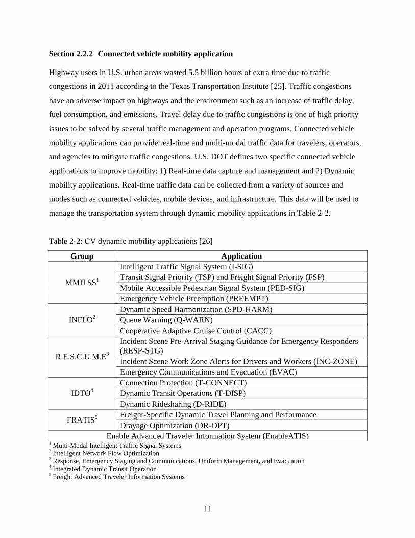
Section 2.2.2 Connected vehicle mobility application

Highway users in U.S. urban areas wasted 5.5 billion hours of extra time due to traffic

congestions in 2011 according to the Texas Transportation Institute [25]. Traffic congestions

have an adverse impact on highways and the environment such as an increase of traffic delay,

fuel consumption, and emissions. Travel delay due to traffic congestions is one of high priority

issues to be solved by several traffic management and operation programs. Connected vehicle

mobility applications can provide real-time and multi-modal traffic data for travelers, operators,

and agencies to mitigate traffic congestions. U.S. DOT defines two specific connected vehicle

applications to improve mobility: 1) Real-time data capture and management and 2) Dynamic

mobility applications. Real-time traffic data can be collected from a variety of sources and

modes such as connected vehicles, mobile devices, and infrastructure. This data will be used to

manage the transportation system through dynamic mobility applications in Table 2-2.

Table 2-2: CV dynamic mobility applications [26]

Group Application

MMITSS1

Intelligent Traffic Signal System (I-SIG)

Transit Signal Priority (TSP) and Freight Signal Priority (FSP)

Mobile Accessible Pedestrian Signal System (PED-SIG)

Emergency Vehicle Preemption (PREEMPT)

INFLO2

Dynamic Speed Harmonization (SPD-HARM)

Queue Warning (Q-WARN)

Cooperative Adaptive Cruise Control (CACC)

R.E.S.C.U.M.E3

Incident Scene Pre-Arrival Staging Guidance for Emergency Responders

(RESP-STG)

Incident Scene Work Zone Alerts for Drivers and Workers (INC-ZONE)

Emergency Communications and Evacuation (EVAC)

IDTO4

Connection Protection (T-CONNECT)

Dynamic Transit Operations (T-DISP)

Dynamic Ridesharing (D-RIDE)

FRATIS5

Freight-Specific Dynamic Travel Planning and Performance

Drayage Optimization (DR-OPT)

Enable Advanced Traveler Information System (EnableATIS) 1 Multi-Modal Intelligent Traffic Signal Systems

2 Intelligent Network Flow Optimization

3 Response, Emergency Staging and Communications, Uniform Management, and Evacuation

4 Integrated Dynamic Transit Operation

5 Freight Advanced Traveler Information Systems

12

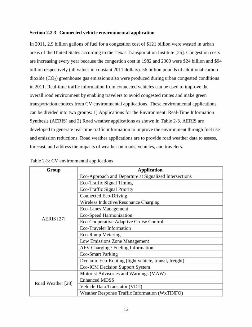
Section 2.2.3 Connected vehicle environmental application

In 2011, 2.9 billion gallons of fuel for a congestion cost of $121 billion were wasted in urban

areas of the United States according to the Texas Transportation Institute [25]. Congestion costs

are increasing every year because the congestion cost in 1982 and 2000 were $24 billion and $94

billion respectively (all values in constant 2011 dollars). 56 billion pounds of additional carbon

dioxide (CO2) greenhouse gas emissions also were produced during urban congested conditions

in 2011. Real-time traffic information from connected vehicles can be used to improve the

overall road environment by enabling travelers to avoid congested routes and make green

transportation choices from CV environmental applications. These environmental applications

can be divided into two groups: 1) Applications for the Environment: Real-Time Information

Synthesis (AERIS) and 2) Road weather applications as shown in Table 2-3. AERIS are

developed to generate real-time traffic information to improve the environment through fuel use

and emission reductions. Road weather applications are to provide road weather data to assess,

forecast, and address the impacts of weather on roads, vehicles, and travelers.

Table 2-3: CV environmental applications

Group Application

AERIS [27]

Eco-Approach and Departure at Signalized Intersections

Eco-Traffic Signal Timing

Eco-Traffic Signal Priority

Connected Eco-Driving

Wireless Inductive/Resonance Charging

Eco-Lanes Management

Eco-Speed Harmonization

Eco-Cooperative Adaptive Cruise Control

Eco-Traveler Information

Eco-Ramp Metering

Low Emissions Zone Management

AFV Charging / Fueling Information

Eco-Smart Parking

Dynamic Eco-Routing (light vehicle, transit, freight)

Eco-ICM Decision Support System

Road Weather [28]

Motorist Advisories and Warnings (MAW)

Enhanced MDSS

Vehicle Data Translator (VDT)

Weather Response Traffic Information (WxTINFO)

13

Section 2.3 Measurement of the Performance of Connected Vehicle and Applications

Section 2.3.1 Traffic information propagation distance

The performance of connected vehicle systems and applications needs to be measured to assess

the feasibility of available connected vehicle applications. Various measurements are used to

investigate the performance of connected vehicle systems. Some studies have used information

propagation via wireless communication to measure the performance of V2V communication.

The further and quicker propagation of traffic incident information is important for traffic

incident management because traffic incidents cause secondary incidents, and about 20 percent

of all incidents are secondary incidents [29]. If an incident or mechanical breakdown on the link

disables a vehicle, this information needs to be delivered to approaching traffic far and quickly.

Shladover et al. [30] used an average wireless message propagation distance to measure the

performance of cooperative vehicle systems (CVS) based on the market penetration rate of

equipped vehicles and traffic density. The distance of message propagation increased as the

market penetration rate of equipped vehicles and traffic density increased. This distance of

message propagation also increased rapidly as the ratio of the communication range to the mean

separation between vehicles increased. Jung et al. [31] studied the performance of inter-vehicle

communications (IVC) using a communication network simulator (ns-2). The information

propagation distance was measured to investigate the success rate by setting one vehicle as an

information source. Results showed that the average maximum information propagation

distances generally increase as the transmission range increases, because shorter transmission

range and low traffic density negatively affects the message propagation in IVC over multiple

vehicles. However, this study considered only one level (10%) of market penetration level for

equipped vehicles. Yang and Recker tested traffic information propagation and probability of

communication success in freeway and arterial networks within a simulation framework [32].

The maximum information propagation distance was measured based on various combinations

with market penetration rate of IVC-capable vehicle, communication radius range, traffic

conditions, and level of service (LOS) under incident conditions. This study also used a

hypothetical study area with a simple grid network.

14

Section 2.3.2 Real-time traffic information estimation

Connected vehicles can be used as probe vehicles to monitor and control real-time traffic

information such as travel time, speed, and delay for various traffic management and traveler

information applications. The estimation error of real-time traffic information estimated by

connected vehicles can be used to measure the performance of connected vehicle systems and

applications. Some previous studies used the error rate of travel time estimated by connected

vehicles to measure the performance of connected vehicle systems. Rim et al. estimated lane-

level travel times for traffic information systems using V2V and V2I communications [33]. The

error rate of travel time estimation is 6% to 9% when the penetration of equipped vehicles is

more than 20%. This study collected trajectory data of individual vehicles in 7.42 km of

simulation (VISSIM) network with realistic highway geometric conditions and traffic conditions.

Li et al. used vehicle–infrastructure integration probe data to measure real-time arterial

performance [34]. The traffic information was collected through V2I communication in a six-

intersection arterial simulation model using VISSIM. The average travel time was used as the

major measure of effectiveness (MOE) of traffic conditions and the average absolute estimation

error percentage for the conventional point-based detection model in this study was 13.9%. Their

VII probe data based model was performed better although probe vehicle penetration rate is 5%.

Oh et al. evaluated the performance of travel time estimation models using GPS and V2V

communications under normal and incident traffic conditions [35]. The V2V communication

range, the market penetration rate of equipped vehicles, and the travel time aggregation interval

were investigated as the functional requirements.

The speed estimation error by connected vehicles has also been used to assess the

performance of connected vehicle applications or real-time traffic information systems using

probe vehicles. Argote et al. used connected vehicle data to develop estimation methods for

measures of effectiveness (MOEs) and determine the required penetration rates for each MOE:

average speed, delay, number of stops, and acceleration noise [36]. The average speed was

estimated by the total distance traveled and total time spent of connected vehicles. The average

speed can be estimated accurately when the penetration rate is higher than 50% within a 10% of

the error. Li et al. developed a probe sample size model to estimate an average link speed using

different penetration rates of probe vehicles, speed estimation interval, and probe report interval

15

[37]. The average link speed was more accurate as the penetration rate of probe vehicles

increased and probe report interval decreased.

Connected vehicle technology can be applied to reduce travel delay at signalized

intersections by signal control applications. Hu, Park, and Parkany developed a new transit signal

priority (TSP) method using connected vehicle technology based on two-way communications

between transit buses and the traffic signal controller [38]. Results showed that their TSP model

reduced bus delays up to about 90% compared with no-TSP condition in VISSIM simulation

when the congestion level is low. But, benefit of this TSP model was decreased as the congestion

level is increased. Another research also considered cooperative bus priority system in connected

vehicle environment [39]. The number of stops and the travel time of buses were decreased by

optimizing bus priority signal timings, bus speed, and bus holding times at bus stops using real

traffic information from connected vehicle technology.

Li et al. used connected vehicle technology to real-time estimate queue length from probe

trajectory (with loop detector data) and signal timing data [40]. The estimation accuracy of queue

length was examined under different market penetration rates. Mean absolute percentage error

(MAPE) for queue length was less than 18% when the penetration rate was 50%. But, MAPE

was much increased to around 60% in a very low penetration rate (10%). One study presented a

queue spillback detection methods and signal control strategy to mitigate queue spillbacks [41].

Data from connected vehicles was used to avoid the occurrence of spillbacks within the next

cycle in the queue spillback detection. At least 20% of the penetration rate was required for

accurate queue detection.

Connected vehicle technology was used to estimate the positions of unequipped vehicles

on a signalized arterial [42]. The results showed the performance of connected vehicle mobility

applications can be improved in a low penetration rate of connected vehicle environment because

of the location estimation algorithm for unequipped vehicles.

Section 2.3.3 Environmental impact

Improvement of the environment is one of objectives of connected vehicle research and

environmental impacts by connected vehicle are used to measure the performance of connected

vehicle systems and applications. Bhavsar et al. tested three optimization strategies to minimize

16

the energy consumption based on different types of information availability with the use of

connected vehicle technology (CVT) [43]. A linear relation was found between energy savings

and the penetration rate of CVT in the case study network. Fuel consumption was decreased by

31% to 35% when both signal timing and headway information were provided with a 30%

penetration of CVT at the peak hour volume. Kamalanathsharmaa and Rakha developed the eco-

cooperative adaptive cruise control application to minimize the vehicle's fuel consumption in the

Vicinity of Signalized Intersections [44]. V2I communication was applied to receive signal

phasing and timing data, predict vehicles’ trajectory. The fuel consumption was decreased by 5

to 30% in the vicinity of signalized intersections by this application. Ahn and Rakha investigated

the feasibility of ecolane applications to improve the environmental impacts through lane

management strategies [45]. This study evaluated various ecolane algorithms and speed

harmonization applications in INTEGRATION software. Results indicated that the ecolane

systems could improve fuel consumption and air quality resulting from reducing average vehicle

travel time and total delay.

Section 2.3.4 Area coverage

Area coverage can be used as one of measurement to determine the required market penetration

rate or sample size for probe vehicles. Kianfar and Edara used a network coverage index to

measure the performance of methodology to determine the optimal placement of roadside

equipment (RSE) for travel time estimation under V2I communication environment [46]. The

network coverage index was calculated by both travel time error and the number of covered links

by V2I communication based on various market penetration rates and travel time estimation

intervals. Coverage index values were getting better as penetration rates were higher and

estimation intervals were larger. Ygnace et al. developed an area coverage equation for probe

vehicles used in San Francisco to estimate travel times as follows [47]:

E = 1 – exp (-α ρ L) (1)

where E is the coverage, α is the fraction of vehicles sampled, ρ is the density of traffic per unit

length, and L is the average link length. The coverage was defined as a fraction of links for

which the links have been measured in the time frame of interest. This equation translates that

the fraction of vehicles sampled or average link length should be increased to improve the

17

coverage. But, this model did not consider the location error or the link type. Srinivasan and

Jovanis developed a heuristic algorithm for determining number of probe vehicles required in

urban network for reliability of travel time estimation and adequacy of area coverage [48]. This

study indicated a greater proportion of freeway links than of major arterials can reliably be

covered with a given number of probes. Also, the number of probes required increases as the

desired proportion of link coverage in the network increases. BMW Group considered the

potential of vehicle-generated traffic data acquisition for the generation of traffic information and

local hazard warnings [49]. A method for estimating the required floating car penetration rates

on the basis of traffic volume and arrival probabilities is presented. This study showed the

necessary penetration rates for different road network categories. For example, at least 10% of

penetration rate is required for federal roads and urban arterials in peak hours.

18


1. Steven E. Shladover, Gungor Polatkan, Raja Sengupta, Joel VanderWerf, Mustafa Ergen, and

Benedicte Bougler. Dependence of Cooperative Vehicle System Performance on Market

Penetration. Transportation Research Record: Journal of the Transportation Research Board,

No. 2000, Transportation Research Board of the National Academies, Washington, D.C., 2007,

pp. 121–127.

2. Cheol Oh, Taehyung Kim, Wonkyu Kim, Seungpyo Hong, and Junhyeong Park. Capability-

Enhanced Probe Vehicle Surveillance System with Vehicle-to-Vehicle Communications.

Transportation Research Record: Journal of the Transportation Research Board, No. 2189,

Transportation Research Board of the National Academies, Washington, D.C., 2010, pp. 8–16.

3. Bing Mei, Hyejung Hu, Nagui M. Rouphail, and Jae-Joon Lee. Simulation Model for Studying

Impact of Vehicle-to-Vehicle Wireless Communications on Traffic Network Operations.


Transportation Research Board of the National Academies, Washington, D.C., 2010, pp. 107–

115.

4. Byungkyu Park and Joyoung Lee. Assessing Sustainability Impacts of Route Guidance System

under Cooperative Vehicle Infrastructure Environment. Proceedings of the 2009 IEEE

International Symposium on Sustainable Systems and Technology. 2009, pp. 1-6.

5. Javier A. Barria and Suttipong Thajchayapong. Detection and Classification of Traffic

Anomalies Using Microscopic Traffic Variables. IEEE Transactions on Intelligent

Transportation Systems, Vol. 12, No. 3, 2011, pp. 695–704.

6. Mustafa Ergen. Critical Penetration for Vehicular Networks. IEEE Communications Letters,

VOL. 14, NO. 5. 2010, pp. 414-416.

7. Turner, S., and D. Holdener. Probe Vehicle Sample Sizes for Real-Time Information: The

Houston Experience. Proceedings of the Vehicle Navigation and Information Systems

Conference, Seattle, Wash., IEEE, 1995, pp. 3–10.

8. Ygnace, J.-L., C. Drane, Y. B. Yim, and R. de Lacvivier. Travel Time Estimation on the San

Francisco Bay Area Network Using Cellular Phones as Probes. UCB-ITS-PWP-2000-18.

California PATH, Richmond. 2000.

19

9. Matthew W. Green, Michael D. Fontaine, and Brian L. Smith. Investigation of Dynamic Probe

Sample Requirements for Traffic Condition Monitoring. Transportation Research Record:

Journal of the Transportation Research Board, No. 1870, TRB, National Research Council,

Washington, D.C., 2004, pp. 55–61.

10. Tetsuhiro Ishizaka and Atsushi Fukuda. Study on the Reliability of Travel Time Estimation

by Probe Vehicle System. Asian Transport Studies, Volume 1, Issue 4, 2011, pp. 424-435.

11. Brian Gallagher, Hidehiko Akatsuka, and Hideaki Suzuki. Wireless Communications for

Vehicle Safety: Radio Link Performance & Wireless Connectivity Methods. IEEE Vehicular

Technology Magazine, Volume 1, Issue 4, 2006, pp. 4–24.

12. Rui Meireles, Mate Boban, Peter Steenkiste, Ozan Tonguz, and Joao Barros. Experimental

Study on the Impact of Vehicular Obstructions in VANETs. IEEE Vehicular Networking

Conference. 2010, pp. 338-345.

13. ITS Standards Fact Sheets. ASTM E2213-03 - Standard Specification for

Telecommunications and Information Exchange Between Roadside and Vehicle Systems - 5

GHz Band Dedicated Short Range Communications (DSRC) Medium Access Control

(MAC) and Physical Layer (PHY) Specifications.

http://www.standards.its.dot.gov/fact_sheetp.asp?f=66. Accessed August 1, 2014.

14. ITS Standards Fact Sheets. IEEE 1609 - Family of Standards for Wireless Access in

Vehicular Environments (WAVE). http://www.standards.its.dot.gov/fact_sheet.asp?f=80.

Accessed August 1, 2014.

15. USDOT Connected Vehicle Research Program: Vehicle-to-Vehicle Safety Application

Research Plan. Publication DOT HS 811 373. NHTSA, U.S. Department of Transportation,

2011.

16. The CAMP Vehicle Safety Communications Consortium. Vehicle Safety Communications

Project Task 3 Final Report: Identify Intelligent Vehicle Safety Applications Enabled by

DSRC. Publication DOT HS 809 859. NHTSA, U.S. Department of Transportation, 2005.

17. Research and Innovative Technology Administration Webpage. Connected Vehicle Research.

http://www.its.dot.gov/connected_vehicle/connected_vehicle.htm. Accessed July 1, 2014.

18. CVRIA Webpage. Connected Vehicle Applications.

http://www.iteris.com/cvria/html/applications/applications.html. Accessed March 31, 2015.

20

19. Rex Chen, Wen-Long Jin, and Amelia Regan. Broadcasting Safety Information in Vehicular

Networks: Issues and Approaches. IEEE Network, Vol. 24, No. 1, 2010, pp. 20–25.

20. TRAFFIC SAFETY FACTS: 2013 Motor Vehicle Crashes. Publication DOT HS 812 101.


21. Centers for Disease Control and Prevention. Number of deaths for leading causes of death.

http://www.cdc.gov/nchs/fastats/deaths.htm. Accessed March 31, 2015.

22. The Economic Impact of Motor Vehicle Crashes, 2000. Publication DOT HS 809 446.


23. Intelligent Transportation Systems Joint Program Office Webpage. V2V Safety applications.

http://www.its.dot.gov/pilots/pilots_v2v.htm. Accessed March 31, 2015.

24. ITS JPO Webpage. V2I Safety applications. http://www.its.dot.gov/pilots/pilots_v2i.htm.


25. Texas A&M Transportation Institute. 2012 URBAN MOBILITY REPORT. 2012.

26. ITS JPO Webpage. Mobility applications. http://www.its.dot.gov/pilots/pilots_mobility.htm.


27. ITS JPO Webpage. Environment applications.

http://www.its.dot.gov/pilots/pilots_environment.htm. Accessed March 31, 2015.

28. ITS JPO Webpage. Road Weather applications.

http://www.its.dot.gov/pilots/pilots_roadweather.htm. Accessed March 31, 2015.

29. Federal Highway Administration Office of Operations Webpage. Traffic Incident

Management. www.ops.fhwa.dot.gov/aboutus/one_pagers/tim.htm. Accessed July 1, 2014.



Penetration. In Transportation Research Record: Journal of the Transportation Research

Board, No. 2000, Transportation Research Board of the National Academies, Washington,

D.C., 2007, pp. 121–127.

31. Jaeyoung Jung, Rex Chen, Wenlong Jin, R. Jayakrishnan, and Amelia C. Regan. An

Empirical Study of Inter-Vehicle Communication Performance Using NS-2. University of

California Transportation Center. August 2010. http://www.uctc.net/research/papers/UCTC-

FR-2010-33.pdf. Accessed July 1, 2014.

21

32. X. Yang and W. Recker. Simulation Studies of Information Propagation in a Self-Organizing

Distributed Traffic Information System. Transportation Research Part C, Vol. 13, No. 5–6,

2005, pp. 370–390.

33. Heesub Rim, Cheol Oh, Kyungpyo Kang, and Seongho Kim. Estimation of Lane-Level

Travel Times in Vehicle-to-Vehicle and Vehicle-to-Infrastructure-Based Traffic Information

System. In Transportation Research Record: Journal of the Transportation Research Board,

No. 2243, Transportation Research Board of the National Academies, Washington, D.C.,

2011, pp. 9–16.

34. Meng Li, Zhi-jun Zou, Fanping Bu, and Wei-Bin Zhang. Application of Vehicle

Infrastructure Integration Data on Real-Time Arterial Performance Measurements. Presented

at 87th Annual Meeting of the Transportation Research Board, Washington, D.C., 2008.

35. Cheol Oh, Taehyung Kim, Wonkyu Kim, Seungpyo Hong, and Junhyeong Park. Capability-

Enhanced Probe Vehicle Surveillance System with Vehicle-to-Vehicle Communications. In


Transportation Research Board of the National Academies, Washington, D.C., 2010, pp. 8–

16.

36. Juan Argote, Eleni Christofa, Yiguang Xuan, and Alexander Skabardonis. Estimation of

Measures of Effectiveness Based on Connected Vehicle Data. 14th International IEEE

Conference on Intelligent Transportation Systems, Washington, D.C., October, 2011, pp.

1767-1772.

37. Wang Li, Zhang Hai1, Yu Guizhen, and FAN Yaozu. Study of Probe Sample Size Model in

Probe Vehicle Technology. Journal of Transportation Systems Engineering and Information

Technology. Vol. 7, No. 5, 2007, pp. 31-36.

38. Jia Hu, Byungkyu (Brian) Park, and A. Emily Parkany. Transit Signal Priority with

Connected Vehicle Technology. In Transportation Research Record: Journal of the

Transportation Research Board, No. 2418, Transportation Research Board of the National

Academies, Washington, D.C., 2014, pp. 20–29.

39. Yinsong Wang, Wanjing Ma, Wei Yin, and Xiaoguang Yang. Implementation and Testing of

Cooperative Bus Priority System in Connected Vehicle Environment. In Transportation

Research Record: Journal of the Transportation Research Board, No. 2424, Transportation

Research Board of the National Academies, Washington, D.C., 2014, pp. 48–57.

22

40. Jing-Quan Li, Kun Zhou, Steven E. Shladover, and Alexander Skabardonis. Estimating

Queue Length Under Connected Vehicle Technology: Using Probe Vehicle, Loop Detector,

and Fused Data. In Transportation Research Record: Journal of the Transportation Research


D.C., 2013, pp. 17–22.

41. Eleni Christofa, Juan Argote, and Alexander Skabardonis. Arterial Queue Spillback

Detection and Signal Control Based on Connected Vehicle Technology. In Transportation

Research Record: Journal of the Transportation Research Board, No. 2356, Transportation

Research Board of the National Academies, Washington, D.C., 2013, pp. 61–70.

42. Noah J. Goodall, Byungkyu Park, and Brian L. Smith. Microscopic Estimation of Arterial

Vehicle Positions in a Low-Penetration-Rate Connected Vehicle Environment. Journal of

Transportation Engineering. Vol. 140, No. 10, 2014.

43. Parth Bhavsar, Yiming He, Mashrur Chowdhury, Ryan Fries, and Andrew Shealy. Energy

Consumption Reduction Strategies for Plug-In Hybrid Electric Vehicles with Connected

Vehicle Technology in Urban Areas. In Transportation Research Record: Journal of the



44. Raj Kishore Kamalanathsharma and Hesham A. Rakha. Leveraging Connected Vehicle

Technology and Telematics to Enhance Vehicle Fuel Efficiency in the Vicinity of Signalized

Intersections. In Journal of Intelligent Transportation Systems, 2014.

45. Kyoungho Ahn and Hesham A. Rakha. Ecolane Applications: Preliminary Testing and

Evaluation. In Transportation Research Record: Journal of the Transportation Research


D.C., 2014, pp. 41–53.

46. Jalil Kianfar and Praveen Edara. Placement of Roadside Equipment in Connected Vehicle

Environment for Travel Time Estimation. In Transportation Research Record: Journal of the



47. Ygnace, J.-L., C. Drane, Y. B. Yim, and R. de Lacvivier. Travel Time Estimation on the San

Francisco Bay Area Network Using Cellular Phones as Probes. UCB-ITS-PWP-2000-18.

California PATH, Richmond. 2000.

23

48. Karthik K. Srinivasan and Paul P. Jovanis. Determination of Number of Probe Vehicles

Required for Reliable Travel Time Measurement in Urban Network. Transportation Research

Record 1517, 1996, pp. 15-22.

49. Susanne Breitenberger, Bernhard Grüber, Martina Neuherz and Ronald Kates. Traffic

information potential and necessary penetration rates. BMW Group. 2004.

24

Chapter 3 INVESTIGATION OF CAPABILITY OF V2V

COMMUNICATION

Section 3.1 Title

Area Coverage provided by Vehicle-to-Vehicle Communication in an Urban Network

Section 3.2 Abstract

The information obtained from Connected Vehicles has the potential of providing local and area-

wide traffic management solutions which is desperately needed in most large urban areas. The

reliability and the frequency of this transmitted information have to be addressed to ensure that

the users can properly utilize this information to solve traffic management issues. This research

investigates the area covered in space and in time by vehicle to vehicle (V2V) communication in

an urban network based on different market penetration rates of equipped vehicles and wireless

communication coverage in TRANSIMS. The percentage of valid connected vehicles and area

coverage level are used to assess the communication duration rate and spatial-temporal

dispersion of connected vehicles. Results show that both average communication duration rate

and area coverage level increase as the market penetration rate and wireless communication

coverage increase. The communication duration rate of connected vehicles is more sensitive to

the wireless communication coverage than the market penetration rate. However, the market

penetration rate of equipped vehicles has a greater influence on spatial-temporal dispersion of

connected vehicles and the Selected Links case has higher average area coverage level than the

Whole Network case. The average area coverage also varies by time of day and is sensitive to the

density of traffic and to the aggregation level. Finally, the spatial-temporal dispersion of

connected vehicles increase as the density of traffic increases, i.e. more equipped vehicles are

able to communicate with one another. These study findings will be useful for making decisions

about investments in cooperative vehicles in relation to the expected increase in traffic

efficiency.

25

Section 3.3 Introduction

Connected Vehicle research has emerged as one of the highest priorities in the transportation

field. It focuses on Vehicle-to-Vehicle (V2V) and Vehicle-to-Infrastructure (V2I)

communication using wireless technologies such as Dedicated Short Range Communications

(DSRC). Most of the automakers and a number of countries are developing Connected Vehicle

applications. The intent of connected vehicle is to support safety, mobility, and environmental

impact that benefit the users and providers of the transportation system. Connected Vehicles can

provide continuous real-time connectivity to all system users to/from vehicles, infrastructure,

wireless devices, and transportation management centers. The vehicles equipped with V2V

communication system can exchange their data between nearby vehicles such as position, speed,

and location data. V2V communication enables a connected vehicle to avoid crashes by

receiving warning threats or hazards. V2I wireless communication enables a connected vehicle

to exchange safety and operational data with highway infrastructure.

The information obtained from connected vehicles, whether from V2V or V2I, has the

potential of providing local and area-wide traffic management solutions which are desperately

needed in most large urban areas. The reliability and the frequency of this transmitted

information have to be addressed to ensure that the users can properly utilize this information to

solve traffic management issues. This research focuses on the area covered in space and in time

by V2V communication in an urban network based on different market penetration rates and

wireless communication coverage. The findings will be useful for making decisions about

investments in cooperative vehicles in relation to the expected increase in traffic efficiency.

The literature covers a wide range of topics in the connected vehicle research. It is

ubiquitous and is not possible to cite it all in this condensed report. However, the authors will

focus on selected publications that cover the areas of communications and standards and on

issues related to penetration levels of Connected Vehicles and related research work conducted

on probe vehicles and the requirements needed to obtain reliable information for traffic

management purposes. Many countries are working on developing DSRC technology for various

connected vehicle applications to improve safety and mobility.

Estimating required market penetration rate of targeted or probe vehicles to get reliable

results is one of the most major factors for the potential deployment of new transportation

application or service like connected vehicle. Area coverage is an important measurement to

26

determine the required market penetration rate. Although some previous studies on area coverage

were conducted, they were mainly hypothetical and didn’t use realistic and large networks. They

used a cumulative area coverage level by short time durations such as 5, 10, and 15 minutes and

low penetration rate such as 5%. To obtain much more fine grained area coverage level from

shorter time interval, such as 1 minute and 1 second intervals, with higher time duration should

be determined to get better real-time information service

Section 3.4 Study Background

Section 3.4.1 Objectives

The objectives of this research are as follows;

• Identify valid communication among the identified equipped vehicles in the realistic and large

network based on various scenarios of wireless communication coverage and market penetration

rates of equipped vehicles.

• Determine the success and duration rate of wireless communication among the identified

equipped vehicles based on various scenarios

• Determine the dispersion of connected vehicles in time and in space in an urban network

• Calculate the area coverage obtained by the valid communication among equipped vehicles for

the different scenarios stated above.

Section 3.4.2 Overview of TRANSIMS

To assess the dispersion of connected vehicles in time and in space requires a special simulation

that can trace each individual vehicle in an urban area on a second by second basis and be able to

carry the identity of each driver and passenger with it at all time. The simulation that can execute

these requirements is TRANSIMS (Transportation Analysis and Simulation System) which is

developed by Federal Highway Administration (FHWA), USA and is available in the public

domain. The underlying TRANSIMS philosophy is that to study the transportation system’s

performance effectively, one needs to simulate travel in a study area with a rather fine temporal

and spatial resolution. Other research and developmental efforts have also come to the

conclusion that the next generation of urban travel models should be based on micro-analytic

simulation and that they should employ the activity-based approach for modeling travel demand.

27

TRANSIMS differs from current travel demand forecasting methods in its underlying concepts

and structure. These differences include a consistent and continuous representation of time; a

detailed representation of persons and households; time-dependent routing; and a person-based

microsimulator. TRANSIMS microsimulator is the only simulation tool that maintains the

identity of the traveler throughout the simulation, and is capable of accessing the database of

each individual (e.g., income, age, trip purpose, etc.). In other words, it traces the movement of

people as well as vehicles on a second-by-second basis. In addition, TRANSIMS route planner

utilizes a time-dependent, individually-based route choice model that is suitable for considering

each individual response to the value of the travel information provided.

TRANSIMS consists of a series of modules that produce synthetic households, activities

for individuals within each household, the choice of routes for movements among these

activities, and the microsimulation of these movements to create traffic dynamics on the

network, and to estimate the consequent emissions produced. The framework of TRANSIMS, as

shown in Figure 3-2, allows each module to be executed in any desired order by a set of scripts

specified by the user in the Feedback Controller. TRANSIMS starts by creating the identity of

individual synthetic travelers and maintains them throughout the entire simulation process. All

synthetic travelers are generated by the Population Synthesizer module using census data, land-

use data, and network data. After the Population Synthesizer module estimates the number of

synthetic households, and the demographic characteristics of each individual in these households

and the locations of these households on the network, the Activity Generator creates an activity

list for each synthetic traveler. These activities include work, shopping, school, etc. These

activity estimations are based on the activity survey demographic characteristics of individuals as

they are obtained from the survey data. In addition, activity times and activity locations are

determined for each individual activity. The Route Planner module next computes combined

route and mode trip plans to accomplish the desired activities of each individual, such as work,

shopping, etc. It uses a modified version of Dijkstra’s algorithm that computes the shortest path

in a time-dependent, label-constrained network. Its unique feature is that it computes the shortest

path in a multi-modal network. The Traffic Microsimulation module uses the intermodal paths

developed in the Route Planner module to perform a regional microsimulation of vehicle

interactions. The microsimulation, which employs the cellular automata principle and network

partitioning to be able to microsimulate large scale transportation networks, continuously

28

computes the operating status, including locations, speeds, and acceleration or deceleration of all

vehicles throughout the simulation period. The output can provide a detailed, second by second

history of every traveler in the system over a 24-hour period. Every motor vehicle in the study

area is monitored in this manner to identify traffic congestion and emission concentrations,

which is done by the Emissions Estimator module. Finally, the Feedback Controller module

manages the feedback of information among the Activity Generator, the Route Planner, and the

Traffic Microsimulator modules of TRANSIMS as shown in Figure 3-2. This feedback controller

module makes decisions such as what percentage of the regional trips should be fed back

between modules, which trips should be fed back, how far back should the trips go for re-

planning, and when to stop iterating to attain a degree of stability in the results.

These unique features of TRANSIMS would allow the analyst to assess the dispersion of

connected vehicles by time and location in an urban area. There is no limit on the size of the

urban area that can be simulated. In addition this system is able to include a detailed highway

network such as the collector and the feeder systems. The equipped vehicles would be assigned

to travelers in the Population Synthesizer Module based on their socio-economic characteristics.

TRANSIMS also can map the location of the equipped vehicles in the network at every second

based on the penetration level assigned in the Population Synthesizer. The transmission power of

the connected vehicles can be varied and used to create contours of vehicle to vehicle (V2V)

coverage, hence giving the analyst the ability to assess the coverage level and the frequency of

the information obtained from the connected vehicles for different penetration scenarios, and

determines the utility of the investment for different vehicle systems deployment levels.

Section 3.5 Research Methodology

Section 3.5.1 Overview of study process

• Study area and network

The city of Alexandria, VA, USA outside of Washington D.C. was used for this study. The size

of study area is around 44 km2 (17 mi

2), bordered by I-395 (Henry G Shirley Memorial

Highway), I-495 (Capital Beltway), and State Route 400 as shown in Figure 3-1. TRANSIMS

provided the dataset for Alexandria as the test case. This dataset includes all the input data

29

needed to represent and code the highway and transit networks. This highway network has 3,653

links and about 420,000 trips.

Figure 3-1: Alexandria study area.

• Distribution of equipped vehicles

Vehicles having a specified vehicle type and subtype in TRANSIMS are assumed as the

equipped vehicles that can communicate with nearby other equipped vehicles to exchange traffic

and travel information among each other. The fraction of equipped vehicles to total vehicles can

be changed in the population synthesizer module of TRANSIMS to represent different market

penetration rates. The population synthesizer module assigns vehicles including equipped

vehicles to each household according to their socio-economic characteristics [1, 2]. Then, the

equipped and non-equipped vehicles are distributed onto the network through the modules of

activity generator, router planner, and microsimulator. Figure 3-2 shows the flowchart of the

study process.

30

Figure 3-2: Study process flowchart.

• Collection of vehicle data

Each individual vehicle trajectory data is required to assess the dispersion of equipped vehicles

in time and space in the study area. TRANSIMS offers detailed snapshot data as one of the

output files from the microsimulator. This snapshot data include the location of each individual

traveler, car, or transit vehicle on a second-by-second basis. Each equipped vehicle can be traced

from the provided snapshot data such as vehicle ID, link ID with direction, lane, vehicle type,

speed, x, y, and z coordinates of each vehicle at specified time points.

• Analysis of vehicle data

This study assumed a valid connected vehicle as the equipped vehicle that is able to

communicate with other equipped vehicle when they are spatially within defined wireless

31

communication coverage distance. After identifying all equipped vehicles using vehicle ID and

vehicle type defined in population synthesizer module, the distances between all equipped

vehicles are calculated using x and y coordinates from snapshot data. The percentage of valid

connected vehicles, the success rate of communication among equipped vehicles, and the area

coverage that they produce, would be used to assess the coverage level and the frequency of the

information obtained from the connected vehicles for different market penetration rates of

equipped vehicles and wireless communication coverage distances.

Section 3.5.2 Scenarios

Nine scenarios are analyzed in this study based on two variables, market penetration rate of

equipped vehicles and wireless communication coverage. Three market penetration rates of

equipped vehicles (10%, 20%, and 40%), and three wireless communication coverage (100m,

200m, and 500m) are evaluated for the two study area networks. In this study the maximum

wireless communication coverage is limited to 500m because some obstructions of wireless

communication such as buildings and large vehicles may be existed in the Alexandria network.

Section 3.6 Results

Section 3.6.1 Communication duration rate of connected vehicles

Several TRANSIMS runs were conducted to utilize the Alexandria data sets provided by FHWA.

As stated earlier, TRANSIMS offers detailed snapshot data as one of the output files. The

vehicle data was collected from the snapshot output file at every one minute during 4 hours from

6:00 to 10:00 a.m. Due to the huge size of the snapshot data file, the aggregation to the 1 minute

level was needed in order to manage the large data for the four hours during the morning peak

period. The total number of vehicles in the whole network is about 111,200 vehicles during four

hours. The one second movement of these vehicles for four hours would have created around 1.2

trillion data points for only one output variable, which would be hard to manage for multiple

variables without utilizing super computers. Besides, the vehicles’ movements in one second are

too small to create any change in the dispersion results of connected vehicles. However, the

authors did organize the data at 10 seconds interval level for a 30 minutes period in order to

gauge the differences in Section 3.6.3.

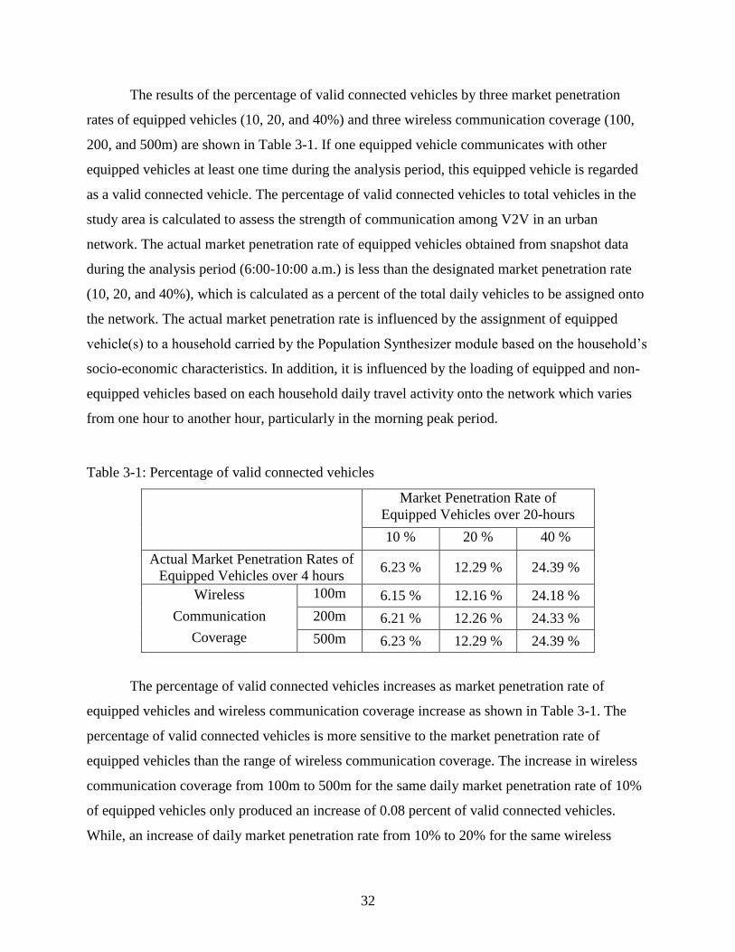
32

The results of the percentage of valid connected vehicles by three market penetration

rates of equipped vehicles (10, 20, and 40%) and three wireless communication coverage (100,

200, and 500m) are shown in Table 3-1. If one equipped vehicle communicates with other

equipped vehicles at least one time during the analysis period, this equipped vehicle is regarded

as a valid connected vehicle. The percentage of valid connected vehicles to total vehicles in the

study area is calculated to assess the strength of communication among V2V in an urban

network. The actual market penetration rate of equipped vehicles obtained from snapshot data

during the analysis period (6:00-10:00 a.m.) is less than the designated market penetration rate

(10, 20, and 40%), which is calculated as a percent of the total daily vehicles to be assigned onto

the network. The actual market penetration rate is influenced by the assignment of equipped

vehicle(s) to a household carried by the Population Synthesizer module based on the household’s

socio-economic characteristics. In addition, it is influenced by the loading of equipped and non-

equipped vehicles based on each household daily travel activity onto the network which varies

from one hour to another hour, particularly in the morning peak period.

Table 3-1: Percentage of valid connected vehicles

Market Penetration Rate of

Equipped Vehicles over 20-hours

10 % 20 % 40 %

Actual Market Penetration Rates of

Equipped Vehicles over 4 hours 6.23 % 12.29 % 24.39 %

Wireless

Communication

Coverage

100m 6.15 % 12.16 % 24.18 %

200m 6.21 % 12.26 % 24.33 %

500m 6.23 % 12.29 % 24.39 %

The percentage of valid connected vehicles increases as market penetration rate of

equipped vehicles and wireless communication coverage increase as shown in Table 3-1. The

percentage of valid connected vehicles is more sensitive to the market penetration rate of

equipped vehicles than the range of wireless communication coverage. The increase in wireless

communication coverage from 100m to 500m for the same daily market penetration rate of 10%

of equipped vehicles only produced an increase of 0.08 percent of valid connected vehicles.

While, an increase of daily market penetration rate from 10% to 20% for the same wireless

33

communication coverage of 100m produced a 6.01% increase in valid connected vehicles. The

market penetration rate has a greater influence on the validity of connected vehicles than the

communication area coverage.

The success rate of communication among equipped vehicles in the study area is shown

in Table 3-2. Unlike the results of the above percentage of valid connected vehicles, these

communication success rates of connected vehicles did not change very much although the

market penetration rate of equipped vehicles and wireless communication coverage did change.

The difference between the minimum and maximum communication success rate of connected

vehicles is 1.24%. At least 98% of equipped vehicles are able to communicate with nearby

equipped vehicles at least one time in this network. They can exchange their information among

one another and get a benefit from V2V based applications at least one time. Eighty two

equipped vehicles among 6,568 equipped vehicles failed to communicate with nearby equipped

vehicles in the case with 10% of market penetration rate and 100m of wireless communication

coverage during 4 hours in the morning peak time. Two hundred and twenty equipped vehicles

among 25,717 equipped vehicles didn’t success to communicate with other equipped vehicles

when the market penetration rate is 40% and wireless communication coverage is 100m. But,

only one equipped vehicle failed to communicate with nearby equipped vehicles when the

wireless communication coverage is 500m with 20% and 40% of market penetration rate. Almost

all equipped vehicles are able to communicate with other equipped vehicles when they are

spatially within 500m of wireless communication coverage regardless of the level of market

penetration rate of equipped vehicles.

Table 3-2: Success rate* of communication among equipped vehicles


Equipped Vehicles

10 % 20 % 40 %

Wireless

Communication

Coverage

100m 98.76 % 98.92 % 99.14 %

200m 99.67 % 99.71 % 99.77 %

500m 100.00 % 99.99 % 100.00 %

*Success rate of communication = (Number of valid connected vehicles / Number of

equipped vehicles) * 100

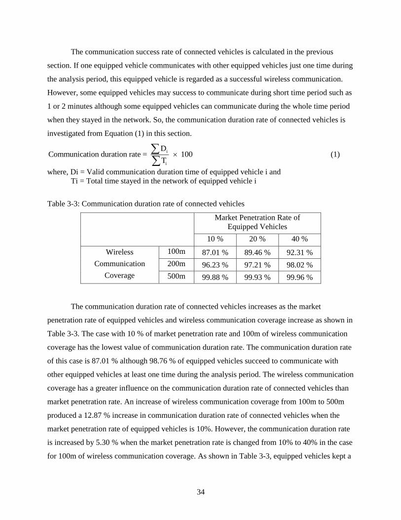
34

The communication success rate of connected vehicles is calculated in the previous

section. If one equipped vehicle communicates with other equipped vehicles just one time during

the analysis period, this equipped vehicle is regarded as a successful wireless communication.

However, some equipped vehicles may success to communicate during short time period such as

1 or 2 minutes although some equipped vehicles can communicate during the whole time period

when they stayed in the network. So, the communication duration rate of connected vehicles is

investigated from Equation (1) in this section.

i

i

DCommunication duration rate = 100

T

(1)

where, Di = Valid communication duration time of equipped vehicle i and

Ti = Total time stayed in the network of equipped vehicle i

Table 3-3: Communication duration rate of connected vehicles


Equipped Vehicles

10 % 20 % 40 %

Wireless

Communication

Coverage

100m 87.01 % 89.46 % 92.31 %

200m 96.23 % 97.21 % 98.02 %

500m 99.88 % 99.93 % 99.96 %

The communication duration rate of connected vehicles increases as the market

penetration rate of equipped vehicles and wireless communication coverage increase as shown in

Table 3-3. The case with 10 % of market penetration rate and 100m of wireless communication

coverage has the lowest value of communication duration rate. The communication duration rate

of this case is 87.01 % although 98.76 % of equipped vehicles succeed to communicate with

other equipped vehicles at least one time during the analysis period. The wireless communication

coverage has a greater influence on the communication duration rate of connected vehicles than

market penetration rate. An increase of wireless communication coverage from 100m to 500m

produced a 12.87 % increase in communication duration rate of connected vehicles when the

market penetration rate of equipped vehicles is 10%. However, the communication duration rate

is increased by 5.30 % when the market penetration rate is changed from 10% to 40% in the case

for 100m of wireless communication coverage. As shown in Table 3-3, equipped vehicles kept a

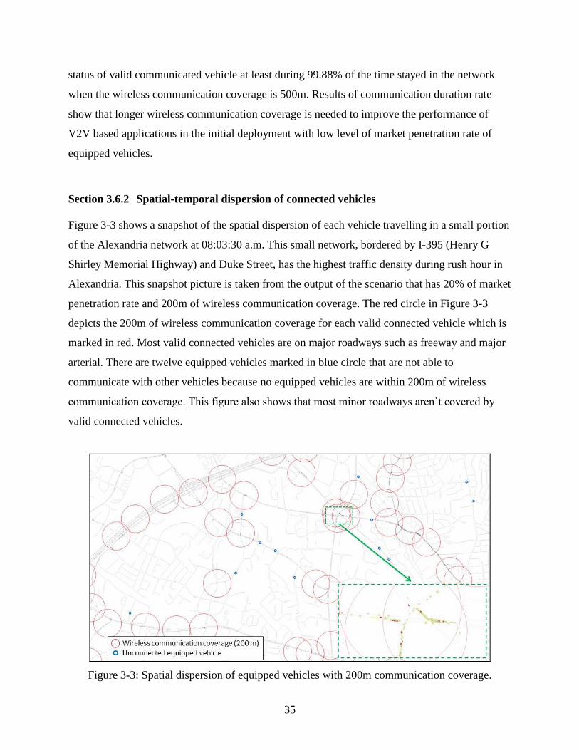
35

status of valid communicated vehicle at least during 99.88% of the time stayed in the network

when the wireless communication coverage is 500m. Results of communication duration rate

show that longer wireless communication coverage is needed to improve the performance of

V2V based applications in the initial deployment with low level of market penetration rate of

equipped vehicles.

Section 3.6.2 Spatial-temporal dispersion of connected vehicles

Figure 3-3 shows a snapshot of the spatial dispersion of each vehicle travelling in a small portion

of the Alexandria network at 08:03:30 a.m. This small network, bordered by I-395 (Henry G

Shirley Memorial Highway) and Duke Street, has the highest traffic density during rush hour in

Alexandria. This snapshot picture is taken from the output of the scenario that has 20% of market

penetration rate and 200m of wireless communication coverage. The red circle in Figure 3-3

depicts the 200m of wireless communication coverage for each valid connected vehicle which is

marked in red. Most valid connected vehicles are on major roadways such as freeway and major

arterial. There are twelve equipped vehicles marked in blue circle that are not able to

communicate with other vehicles because no equipped vehicles are within 200m of wireless

communication coverage. This figure also shows that most minor roadways aren’t covered by

valid connected vehicles.

Figure 3-3: Spatial dispersion of equipped vehicles with 200m communication coverage.

36

The area coverage level of valid connected vehicle is used to assess the spatial-temporal

dispersion of connected vehicles. The concept of area coverage level adopted in this study is

different from the ones used in previous studies that are discussed in the literature review. The

cumulative fraction of number of covered links by probe vehicles was used in previous studies.

Also, if one probe vehicle is on a certain link, this link was assumed to be covered to estimate

travel time or speed. In addition, previous studies only considered short time durations such as 5,

10, and 15 minutes and low penetration rate of probe vehicles such as 5%. This study uses the

average fraction of links covered by platoons of valid connected vehicles over total lengths of all

links in the study area at every 1 minute during 4 hours. Figure 3-4 depicts pictorially the

concept to compute coverage length on a link in this study, where T is the length of link and L is

the length of a platoon of valid connected vehicles.

Figure 3-4: Computation of coverage length on a link.

Table 3-4 shows the average percentage of the study area covered by valid

communication of equipped vehicles for the 3x3 scenarios of market penetration rate and

37

wireless communication coverage. The average area coverage level is the proportion between the

linear lengths of links covered by valid connected vehicles and the total linear lengths of all links

in the study area. This section for the area coverage level considers two different study area

networks; the Whole Network and the Selected Links network. Two freeways, one expressway,

and four major arterials are identified to compose the Selected Links network case in Alexandria

while the Whole Network case covers all the links in the Alexandria network. The Selected

Links network represents the higher functional classification of the roadways which traditionally

carries more than 70 % of all travels at any time of the day and is worthy of studying it as a

separate case.

Table 3-4: Average area coverage level* of connected vehicles

Study Area

Whole Network Selected Links

Market Penetration Rate

of Equipped Vehicles 10 % 20 % 40 % 10 % 20 % 40 %

Wireless

Communication

Coverage

100m 1.39 % 4.08% 8.43 % 2.33 % 8.07 % 19.69 %

200m 2.37 % 5.83 % 10.96 % 4.52 % 12.53 % 26.32 %

500m 3.38 % 7.29 % 12.27 % 7.29 % 16.60 % 30.33 %

* Average area coverage level = (Linear lengths of highways covered by valid connected vehicles / Total linear

lengths of highways in the study area) * 100

The results of area coverage level have a similar pattern with the communication duration

rate that it is increased as the market penetration rate and wireless communication coverage

increased as shown in Table 3-4. But, the average area coverage levels in the Whole Network

case are much lower than results of communication success rate and duration rate presented in

Section 3.6.1. Only 1.39% of links in the Whole Network are covered by valid connected

vehicles when the market penetration rate is 10% and wireless communication coverage is 100m.

The maximum value of the average area coverage levels on Whole Network cases is 12.27%

when the market penetration rate and wireless communication coverage are increased to 40%

and 500m, respectively. The market penetration rate has a greater influence on the average area

coverage level of valid connected vehicles than wireless communication coverage. An increase

of the market penetration rate of equipped vehicles from 10% to 40% produced a 7.04% of

increase in the average area coverage levels in the Whole Network case when the wireless

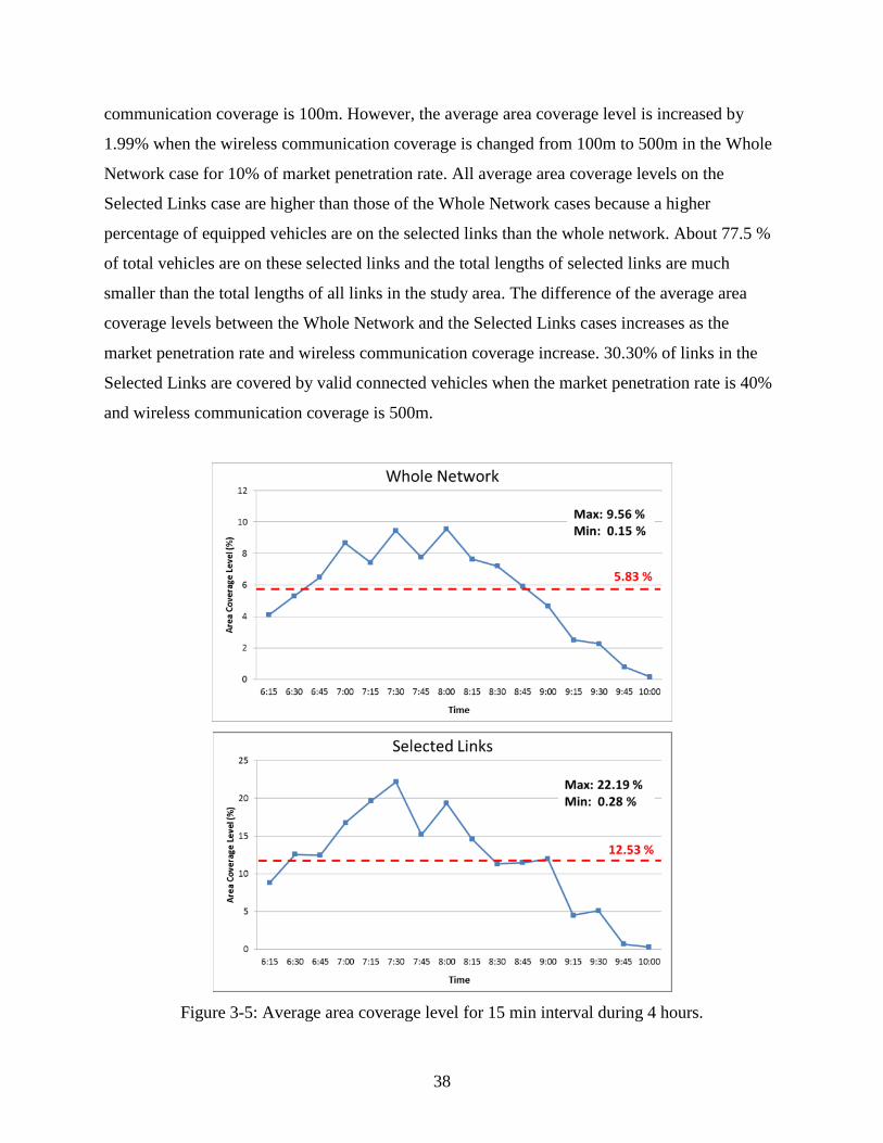
38

communication coverage is 100m. However, the average area coverage level is increased by

1.99% when the wireless communication coverage is changed from 100m to 500m in the Whole

Network case for 10% of market penetration rate. All average area coverage levels on the

Selected Links case are higher than those of the Whole Network cases because a higher

percentage of equipped vehicles are on the selected links than the whole network. About 77.5 %

of total vehicles are on these selected links and the total lengths of selected links are much

smaller than the total lengths of all links in the study area. The difference of the average area

coverage levels between the Whole Network and the Selected Links cases increases as the

market penetration rate and wireless communication coverage increase. 30.30% of links in the

Selected Links are covered by valid connected vehicles when the market penetration rate is 40%

and wireless communication coverage is 500m.

Figure 3-5: Average area coverage level for 15 min interval during 4 hours.

39

The average area coverage level at every 15 minute interval during 4 hours (6:00-10:00

a.m.) is presented to investigate variations of area coverage level in Figure 3-5 for one scenario

having 20% of market penetration rate and 200m of wireless communication coverage. This

figure indicates that the average area coverage varies by time of day and is sensitive to the

density of traffic and to the aggregation level. It shows that the area coverage could be as high as

9.56% at 8:00 a.m. and as low as 0.15% at 10:00 a.m. in the Whole Network case. Also, the

Selected Links case has the higher average area coverage level than Whole Network case.

Section 3.6.3 Spatial-temporal dispersion of connected vehicles using a 10 seconds time

interval

Instead of the one minute update interval that was presented earlier, the authors investigated the

spatial-temporal distribution of connected vehicles using 10 seconds interval for a 30-minute

period from 7:45 a.m. to 8:15 a.m. This 30-minute period was selected because our study area

has the highest traffic density at 8:00 a.m. The 10 seconds update interval would produce higher

density of vehicular traffic which is expected to produce higher percentage of valid wireless

communications among the equipped vehicles. One scenario having 20% of market penetration

rate and 200m of wireless communication coverage was analyzed for this case. The total

numbers of vehicles and equipped vehicles in the Whole Network case are about 21,490 and

2,870 respectively during this 30-minute period, while the numbers of total and equipped

vehicles for the Selected Links case are about 16,360 and 2,370 respectively.

The average area coverage levels for the Whole Network and Selected Links cases are

calculated at every 10 seconds during 30 minutes and the results are shown in Figure 3-6. The

average area coverage levels of valid connected vehicles in the Whole Network and the Selected

Links cases are 8.84 and 18.81 % respectively. Similar to Figure 3-5, this figure shows that the

levels of average area coverage are sensitive to time and density of traffic even at the 10 seconds

intervals. The spatial-temporal dispersion results of connected vehicles during 30 minutes (from

7:45 to 8:15 a.m.) at every 10 seconds in both Whole Network and Selected Links cases are

higher than the previous results obtained during 4 hours (from 6:00 to 10:00 a.m.) as shown in

Table 3-5. Especially, average area coverage levels in both Whole Network and Selected Links

cases are increased by 50 % compared with the previous results from 4 hours analysis. Because,

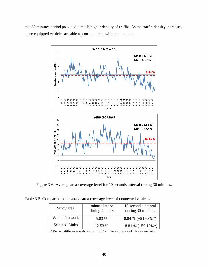
40

this 30 minutes period provided a much higher density of traffic. As the traffic density increases,

more equipped vehicles are able to communicate with one another.

Figure 3-6: Average area coverage level for 10 seconds interval during 30 minutes.

Table 3-5: Comparison on average area coverage level of connected vehicles

Study area 1 minute interval

during 4 hours

10 seconds interval

during 30 minutes

Whole Network 5.83 % 8.84 % (+51.63%*)

Selected Links 12.53 % 18.81 % (+50.12%*)

* Percent difference with results from 1- minute update and 4 hours analysis

41

Section 3.7 Findings

The communication duration rate and spatial-temporal dispersion of connected vehicles for V2V

are investigated based on the market penetration rate of equipped vehicles and wireless

communication coverage in the realistic and large network. The communication duration rate

and average area coverage level increase as the market penetration rate and wireless

communication coverage increase. The percentages of equipped and valid connected vehicles are

calculated to assess the success and duration rate of communication among equipped vehicles.

The communication duration rate of connected vehicles is more sensitive to the wireless

communication coverage than the market penetration rate. Equipped vehicles are able to keep the

status of valid communicated vehicle at least during 99.88% of the time the equipped vehicle

stayed in the network when the wireless communication coverage is 500m.

The area coverage level is used to assess the spatial-temporal dispersion of connected

vehicles for two study areas; the Whole Network and the Selected Links cases. Only 12.27% of

links in the Whole Network are covered by valid connected vehicles when the market penetration

rate is 40% and wireless communication coverage is 500m. The market penetration rate of

equipped vehicles has a greater influence on spatial-temporal dispersion of connected vehicles.

The Selected Links case has higher average area coverage level than the Whole Network case

because a higher percentage of equipped vehicles are on the selected links than on the whole

network and the total lengths of selected links are also much smaller than the total lengths of all

links in the study area. The area coverage varies by time of day and is sensitive to the density of

traffic and to the aggregation level. Finally, the spatial-temporal dispersion of connected vehicles

increase as the density of traffic increases, i.e. more equipped vehicles are able to communicate

with one another. These study findings will be useful for making decisions about investments in

cooperative vehicles.

Future works will include determining the distance of information propagation from one

and multiple information sources through wireless multi-hop. In addition, ownership of equipped

vehicles from a socio-economic aspect will also be considered. Sufficient levels of deployment

of connected vehicle based applications will be determined for obtaining reliable traffic

management solutions.

42

Section 3.8 Acknowledgments

This research was supported by the Mid-Atlantic Universities Transportation Center (MAUTC).

This paper was presented at Urban Transport 2014, Algarve, Portugal, May 2014. We got a

permission to use this paper (DOI. 10.2495/UT140341 entitled "Assessment of Certain

Applications of Vehicle to Vehicle Communication in an urban Network” at Urban Transport

2014, http://www.witpress.com/elibrary/wit-transactions-on-the-built-environment/138/26154)) for my

dissertation.


Most references used in Chapter 3 are listed in Chapter 2 (LITERATURE REVIEW). Only new

references are listed in this section.

1. Hobeika, A.G., et.al.. TRANSIMS – The Population Synthesizer Module, A formal report

submitted to FHWA, Washington, D.C., 2001.

2. Lee, K.S., and Hobeika, A.G.. Application of Dynamic Value Pricing Through Enhancements

to TRANSIMS” Journal of the Transportation Research Board No. 2003, 2007, pp 7-16.

http://www.witpress.com/elibrary/wit-transactions-on-the-built-environment/138/26154

43

Chapter 4 ASSESSMENT OF PERFORMANCE OF V2V APPLICATION

Section 4.1 Title

Assessment of Vehicle-to-Vehicle Communication based Applications in an Urban Network

Section 4.2 Abstract

Connected vehicle technology has the potential to improve safety and mobility for local and

wide-area traffic management. Most previous studies of connected vehicle applications have

used simple and hypothetical networks; measurements in realistic and large networks are

required if connected vehicle applications are to be deployed in the real world. This paper

measures the performance of vehicle-to-vehicle (V2V) applications and determines the required

minimum level of deployment for V2V applications in a large urban network. Distance of

information propagation and speed estimation error are used to measure the performance of

event-driven and periodic applications with different market penetration rates of equipped

vehicles and wireless communication coverage, at both morning peak and non-peak times. As

wireless communication coverage and market penetration rates of equipped vehicles increase,

distance of information propagation increases while speed estimation error decreases in our study

area. For event-driven applications, wireless communication coverage is the major factor

because it has a greater impact on the distance of information propagation. For periodic

applications, however, the market penetration rate of equipped vehicles has a greater impact on

the performance than wireless communication coverage; this is because the speed estimation

error more decreases as the market penetration rate increases. The performance of event-driven

improves in the higher traffic density conditions of peak time while the performance of periodic

application improves in the lower traffic density conditions of non-peak time. The required

minimum level of deployment for each application is determined to obtain reliable traffic

management solutions. These study findings will be useful for deployments of connected

vehicle applications. In particular, event-driven applications can be deployed reliably in the

initial stage of deployment, despite their low level of market penetration.

44

Section 4.3 Introduction

Connected vehicle technology has the potential to improve safety and mobility for local and

wide-area traffic management. Many automotive manufacturers and countries have developed

and evaluated various connected vehicle based applications and services thanks to the

development of wireless communication technology. Connected vehicle applications and

technologies are still in the stage of field testing due to policy and institutional issues. But these

applications may be deployed in the real world soon because the U.S. Department of

Transportation’s (DOT) National Highway Traffic Safety Administration recently issued

advance notice of proposed rulemaking to start implementation of vehicle-to-vehicle (V2V)

communication for light vehicles.

Though various measurements have been used to assess the performance of connected

vehicle applications in previous studies, they have all used hypothetical study areas with simple

networks. Moreover, none of the studies have determined the required minimum level of

deployment of connected vehicle applications based on combinations of various parameters, such

as market penetration rate of equipped vehicles, wireless communication coverage, and traffic

density. Our study assesses the performance of selected applications in a realistic and large

network and determines the required minimum level of deployment for each application in

various scenarios. This chapter is organized as follows. The next section presents the objectives

and approach of this study. The following methodology section explains the study flow,

including selecting study site, identifying equipped and connected vehicles, and measurements

for each application. The results section investigates the performance and required minimum

level of deployment for each application.

Section 4.4 Study approach

Connected vehicle technologies can provide local and area-wide traffic management solutions,

but connected vehicle based applications have not yet been deployed in the real world.

However, many research projects have identified available applications and evaluated their

feasibility. Connected vehicle applications and technologies are still in the stage of field testing

and have been tested under real-world operating conditions at several connected vehicle test

beds. Prior to real-world experiments, simulation study is always conducted to assess the impacts

45

and to define the variables and conditions that needs to be executed in the real world. Most

previous studies used simple and hypothetical networks; a realistic and large network is needed

to further assess the performance of connected vehicle applications. The required minimum level

of deployment for connected vehicle application needs to be determined according to the type of

application. In the early stages of deployment, connected vehicle applications may perform

insufficiently, due to the low market penetration rate of vehicles equipped with wireless

communication devices.

This study has two objectives: 1) to measure the performance of V2V applications and 2)

to determine the required minimum level of deployment for V2V applications. In our previous

study, we developed a simulation model to represent a connected vehicle environment. That

study identified connected vehicles among equipped vehicles with wireless communication

devices in a realistic and large network based on various scenarios with wireless communication

coverage and market penetration rates of equipped vehicles in TRANSIMS [1]. TRANSIMS

differs from current travel demand forecasting methods and software in its underlying concepts

and structure such as a consistent and continuous representation of time; a detailed representation

of persons and households; time-dependent routing; and a person-based microsimulator.

TRANSIMS assigns all vehicles onto the network based on each individual socio-economic

characteristic (e.g., income, age, trip purpose, etc.). It traces the movement of people as well as

vehicles on a second-by-second basis through microsimulator module [2]. TRANSIMS also can

map the location of the individual vehicle in the network at every second based through ArcGIS.

Route planner in TRANSIMS utilizes a time-dependent, individually-based route choice model

that is suitable for considering each individual response to the value of the travel information

provided [3, 4]. This study considers two types of connected vehicle applications: event-driven

and periodic application. The performance of each event-driven and periodic application is

assessed by each selected measurement under 3X3 scenarios with wireless communication

coverage and market penetration rates of equipped vehicles. The required minimum level of

deployment for each application to obtain a reliable traffic management solution is then

determined.

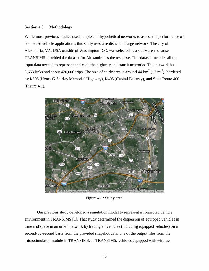
46

Section 4.5 Methodology

While most previous studies used simple and hypothetical networks to assess the performance of

connected vehicle applications, this study uses a realistic and large network. The city of

Alexandria, VA, USA outside of Washington D.C. was selected as a study area because

TRANSIMS provided the dataset for Alexandria as the test case. This dataset includes all the

input data needed to represent and code the highway and transit networks. This network has

3,653 links and about 420,000 trips. The size of study area is around 44 km2 (17 mi

2), bordered

by I-395 (Henry G Shirley Memorial Highway), I-495 (Capital Beltway), and State Route 400

(Figure 4.1).

Figure 4-1: Study area.

Our previous study developed a simulation model to represent a connected vehicle

environment in TRANSIMS [1]. That study determined the dispersion of equipped vehicles in

time and space in an urban network by tracing all vehicles (including equipped vehicles) on a

second-by-second basis from the provided snapshot data, one of the output files from the

microsimulator module in TRANSIMS. In TRANSIMS, vehicles equipped with wireless

47

communication devices are assumed as having a specified vehicle type and subtype. The

equipped vehicles can communicate with nearby equipped vehicles to exchange traffic and travel

information such as speed and location. As connected vehicles, these equipped vehicles receiving

information are also able to relay their information to nearby equipped vehicles within the

wireless communication coverage through a multi-hop based wireless relay (repeater). This study

has other assumptions to represent a connected vehicle environment in TRANSIMS: 1) There are

no obstructions that block wireless communications to guarantee line-of-sight of wireless

communication in the network; 2) The wireless communication used in this study doesn’t have a

packet loss and delay.

Equipped vehicles were distributed onto the network according to different market

penetration rates of equipped vehicles in the population synthesizer module of TRANSIMS.

Valid wireless communication among equipped vehicles was also identified by measuring

distances between all equipped vehicles using x and y coordinates from snapshot data based on

various scenarios with wireless communication coverage and market penetration rates. A

connected vehicle was defined as an equipped vehicle that is able to communicate with another

equipped vehicle when both vehicles are within a defined wireless communication coverage

distance. This study uses the same methodology used in our previous study to identify equipped

vehicles and valid wireless communication.

This study considers two types of connected vehicle applications: event-driven and

periodic application. Two different measurements were calculated to assess the performance of

each connected vehicle application and determine a required minimum scenario for each

application (Figure 4-2). The first measurement is a distance of information propagation to

investigate the performance of event-driven application under incident traffic conditions. One

stopped and equipped vehicle on a selected link, Henry G Shirley Memorial highway in the study

area, was assumed as the disabled vehicle and information source. To represent incident traffic

conditions in TRANSIMS, a land use file among network data was used to block one selected

lane during the incident periods [5]. Then, the snapshot file was updated to add the disabled

equipped vehicle on the blocked lane as an incident information source after finishing the

simulation run of TRANSIMS. After identifying equipped vehicles and valid wireless

communication through MATLAB coding, the distance of incident information propagation

through multi-hop wireless relay was measured at every 10 seconds for 30 minutes by

48

calculating the distance between the disabled vehicle and the last equipped vehicle receiving

incident information from the disabled vehicle. Each distance of information propagation was

measured to investigate the performance of event-driven applications for each scenario with

different market penetration rates and wireless communication coverage.

Figure 4-2: Study flow chart.

Connected vehicles can be used as probe vehicles to estimate real-time traffic

information, such as speed, travel time, and delay. The error rate of real-time information such as

speed or travel time estimated by connected vehicles can be used to measure the performance of

periodic application. The speed estimation error is used as another measurement to investigate

the performance of periodic application under non-incident condition in this study. The snapshot

data includes the speed of each individual car or transit vehicle on a second-by-second basis. The

speed of the selected roadway was estimated by the speed of the connected vehicles. This

49

estimated speed by the connected vehicles was then compared with an observed speed of all

vehicles, in order to calculate the speed estimation error. The speed estimation error was also

calculated based on different market penetration rates and wireless communication coverage.

Finally, the required minimum levels of deployment for both event-driven and periodic

applications were determined according to the proposed methodology. Nine scenarios were

analyzed based on two variables, market penetration rate (10%, 20%, and 40%) of equipped

vehicles and wireless communication coverage (100m, 200m, and 500m) during two different

time periods: morning peak and non-peak times. The wireless communication coverage can be

up to 1,000 meters according to standards for the dedicated short range communications (DSRC)

[6, 7]; but, the maximum wireless communication coverage in this study is limited to 500 meters

because the real network has obstructions such as buildings and heavy vehicles.

Section 4.6 Results

Section 4.6.1 Measurement of the performance of event-driven application

The distance of incident information propagation from one disabled equipped vehicle through

multi-hop wireless relay was measured to investigate the performance of event-driven

application like forward collision warning or road condition warning applications under incident

traffic conditions. To represent the incident situation, we introduced a disabled equipped vehicle

for 30 minutes, from 8:00 to 8:30 a.m. on a selected link, the Henry G. Shirley Memorial

highway in Alexandria. The distance of information propagation for each scenario with different

market penetration rates and wireless communication coverage was then measured every 10

seconds for 30 minutes (8:00-8:30 a.m.) during the morning peak. Each result in this section is

the averaged value from 10 simulation runs in TRANSIMS for each scenario. The average

distance of information propagation during 30 minutes increases as the market penetration rate of

equipped vehicles and wireless communication coverage increase (Table 4-1). The wireless

communication coverage has a greater influence on the distance of information propagation than

the market penetration rate of equipped vehicles. An increase of the wireless communication

coverage from 100m to 200m produces a 1,691% (from 90.7 to 1,625.1 meters) increase in the

average distance of information propagation when the market penetration rate of equipped

vehicles is 10%. However, the average distance of information propagation increases by only

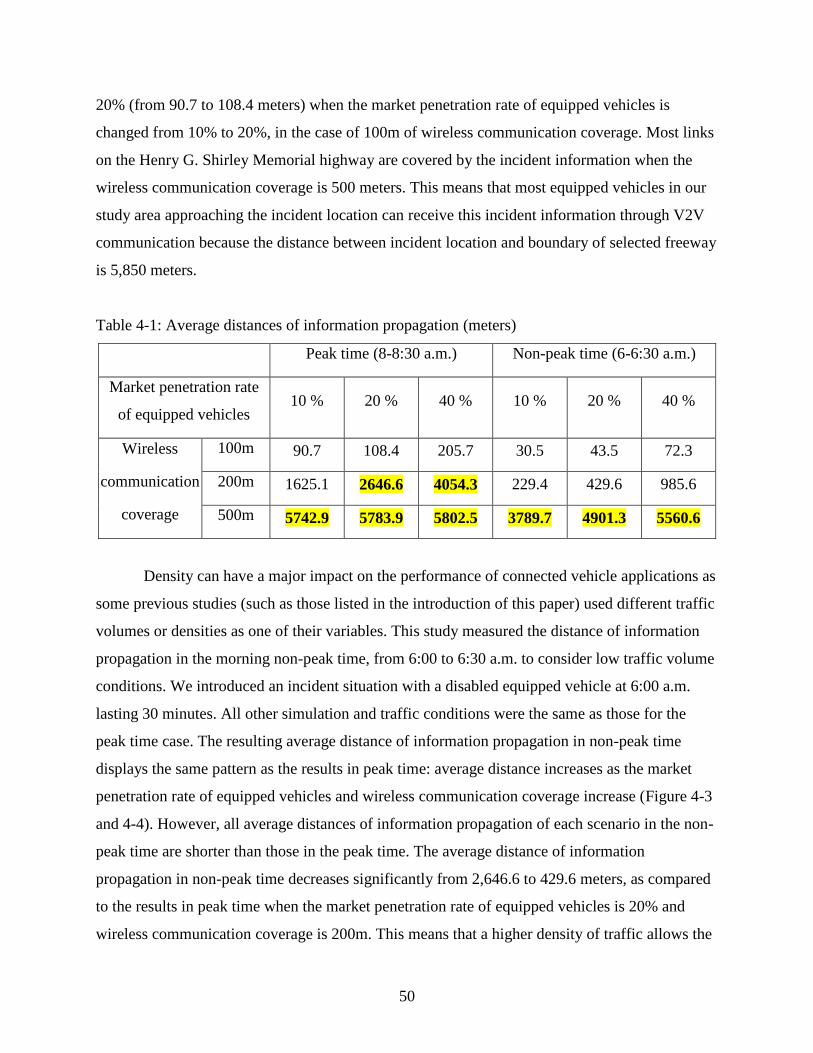
50

20% (from 90.7 to 108.4 meters) when the market penetration rate of equipped vehicles is

changed from 10% to 20%, in the case of 100m of wireless communication coverage. Most links

on the Henry G. Shirley Memorial highway are covered by the incident information when the

wireless communication coverage is 500 meters. This means that most equipped vehicles in our

study area approaching the incident location can receive this incident information through V2V

communication because the distance between incident location and boundary of selected freeway

is 5,850 meters.

Table 4-1: Average distances of information propagation (meters)

Peak time (8-8:30 a.m.) Non-peak time (6-6:30 a.m.)

Market penetration rate

of equipped vehicles 10 % 20 % 40 % 10 % 20 % 40 %

Wireless

communication

coverage

100m 90.7 108.4 205.7 30.5 43.5 72.3

200m 1625.1 2646.6 4054.3 229.4 429.6 985.6

500m 5742.9 5783.9 5802.5 3789.7 4901.3 5560.6

Density can have a major impact on the performance of connected vehicle applications as

some previous studies (such as those listed in the introduction of this paper) used different traffic

volumes or densities as one of their variables. This study measured the distance of information

propagation in the morning non-peak time, from 6:00 to 6:30 a.m. to consider low traffic volume

conditions. We introduced an incident situation with a disabled equipped vehicle at 6:00 a.m.

lasting 30 minutes. All other simulation and traffic conditions were the same as those for the

peak time case. The resulting average distance of information propagation in non-peak time

displays the same pattern as the results in peak time: average distance increases as the market

penetration rate of equipped vehicles and wireless communication coverage increase (Figure 4-3

and 4-4). However, all average distances of information propagation of each scenario in the non-

peak time are shorter than those in the peak time. The average distance of information

propagation in non-peak time decreases significantly from 2,646.6 to 429.6 meters, as compared

to the results in peak time when the market penetration rate of equipped vehicles is 20% and

wireless communication coverage is 200m. This means that a higher density of traffic allows the

51

traffic information to be transmitted farther. About 7,170 vehicles are on Henry G Shirley

Memorial highway during 30 minutes of morning peak time, while there are 4,730 vehicles

during morning non-peak time.

Figure 4-3: Average distances of information propagation (m) in peak time.

Figure 4-4: Average distances of information propagation (m) in non-peak time.

Though some previous studies have used the distance of information propagation to

measure the performance of connected vehicle application, they have not determined the critical

52

level of information propagation distance required to deploy connected vehicle application. One

previous study provided the critical distance of information propagation for cooperative vehicle

system use cases [8]. The range of information or message propagation distance for stopped–

slow vehicle warnings and post-crash notifications to neighboring vehicles is between 50 and

1,500 meters. An information propagation distance of more than 1,500 meters for the event-

driven application in peak time would require a 10% market penetration rate and 200m of

wireless communication coverage (Table 4-1). In other words, at least 200m of wireless

communication coverage are required to deploy the event-driven application, although the

market penetration rate of equipped vehicles can be as low as 10%. During the non-peak time,

the wireless communication coverage should be longer than 500m to operate the event-driven

application.

However, it’s difficult to conclude that the critical distance of information propagation is

1,500 meters for every network, because the distance of information propagation via connected

vehicles also depends on other parameters, such as road networks, traffic pattern, location of

event, and event duration. An individual level of distance of information propagation is needed

for each network having different parameters. The distance between incident location and the

nearest exit on the upstream can be used to determine the critical distance of information

propagation for event-driven application like forward collision warning. The incident

information should be delivered to give warning and detour information to vehicles that are

approaching the incident in the same direction of traffic. The disabled vehicle was located on

Henry G. Shirley Memorial highway (I-395) between Exit 3 and Exit 2 for 30 minutes to

represent the incident situation. The minimum distance of information propagation is 2.5 km for

this study area, because the distance between the incident and first exit on the upstream is 2.5

km. (In other words, approaching drivers can only make a detour to avoid the incident if they

receive the information while they are at least 2.5 km from the incident.) When the critical

distance of information propagation is 2.5 km, the required minimum scenario for event-driven

application in peak time is 20% of market penetration rate and 200m of wireless communication

coverage (Table 4-1). Only three scenarios have a longer distance of information propagation

than 2.5 km during non-peak time. These results show that event-driven application can be

deployed reliably in the early stage of deployment even when the level of market penetration rate

of equipped vehicles is low, as long as wireless communication coverage is longer without

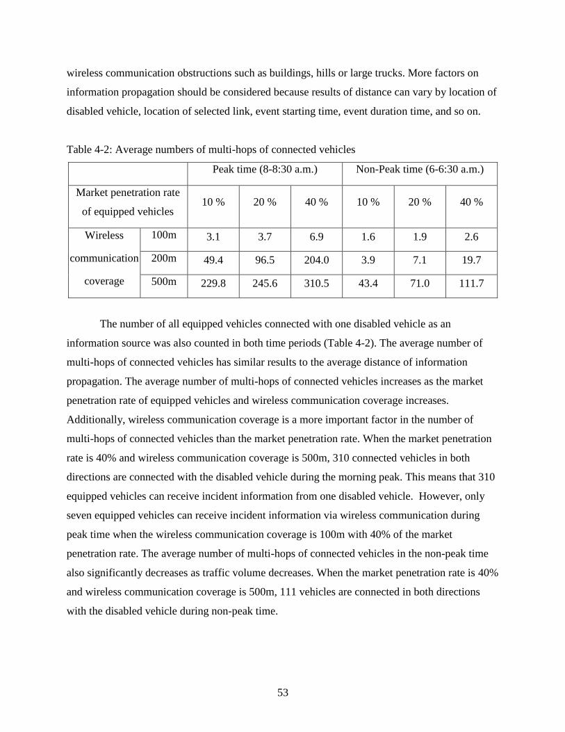
53

wireless communication obstructions such as buildings, hills or large trucks. More factors on

information propagation should be considered because results of distance can vary by location of

disabled vehicle, location of selected link, event starting time, event duration time, and so on.

Table 4-2: Average numbers of multi-hops of connected vehicles

Peak time (8-8:30 a.m.) Non-Peak time (6-6:30 a.m.)



Wireless

communication

coverage

100m 3.1 3.7 6.9 1.6 1.9 2.6

200m 49.4 96.5 204.0 3.9 7.1 19.7

500m 229.8 245.6 310.5 43.4 71.0 111.7

The number of all equipped vehicles connected with one disabled vehicle as an

information source was also counted in both time periods (Table 4-2). The average number of

multi-hops of connected vehicles has similar results to the average distance of information

propagation. The average number of multi-hops of connected vehicles increases as the market

penetration rate of equipped vehicles and wireless communication coverage increases.

Additionally, wireless communication coverage is a more important factor in the number of

multi-hops of connected vehicles than the market penetration rate. When the market penetration

rate is 40% and wireless communication coverage is 500m, 310 connected vehicles in both

directions are connected with the disabled vehicle during the morning peak. This means that 310

equipped vehicles can receive incident information from one disabled vehicle. However, only

seven equipped vehicles can receive incident information via wireless communication during

peak time when the wireless communication coverage is 100m with 40% of the market

penetration rate. The average number of multi-hops of connected vehicles in the non-peak time

also significantly decreases as traffic volume decreases. When the market penetration rate is 40%

and wireless communication coverage is 500m, 111 vehicles are connected in both directions

with the disabled vehicle during non-peak time.

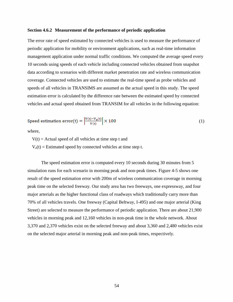
54

Section 4.6.2 Measurement of the performance of periodic application

The error rate of speed estimated by connected vehicles is used to measure the performance of

periodic application for mobility or environment applications, such as real-time information

management application under normal traffic conditions. We computed the average speed every

10 seconds using speeds of each vehicle including connected vehicles obtained from snapshot

data according to scenarios with different market penetration rate and wireless communication

coverage. Connected vehicles are used to estimate the real-time speed as probe vehicles and

speeds of all vehicles in TRANSIMS are assumed as the actual speed in this study. The speed

estimation error is calculated by the difference rate between the estimated speed by connected

vehicles and actual speed obtained from TRANSIM for all vehicles in the following equation:

(1)

where,

V(t) = Actual speed of all vehicles at time step t and

Ve(t) = Estimated speed by connected vehicles at time step t.

The speed estimation error is computed every 10 seconds during 30 minutes from 5

simulation runs for each scenario in morning peak and non-peak times. Figure 4-5 shows one

result of the speed estimation error with 200m of wireless communication coverage in morning

peak time on the selected freeway. Our study area has two freeways, one expressway, and four

major arterials as the higher functional class of roadways which traditionally carry more than

70% of all vehicles travels. One freeway (Capital Beltway, I-495) and one major arterial (King

Street) are selected to measure the performance of periodic application. There are about 21,900

vehicles in morning peak and 12,160 vehicles in non-peak time in the whole network. About

3,370 and 2,370 vehicles exist on the selected freeway and about 3,360 and 2,480 vehicles exist

on the selected major arterial in morning peak and non-peak times, respectively.

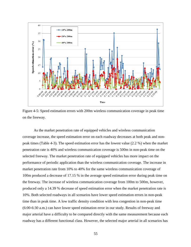
55

Figure 4-5: Speed estimation errors with 200m wireless communication coverage in peak time

on the freeway.

As the market penetration rate of equipped vehicles and wireless communication

coverage increase, the speed estimation error on each roadway decreases at both peak and non-

peak times (Table 4-3). The speed estimation error has the lowest value (2.2 %) when the market

penetration rate is 40% and wireless communication coverage is 500m in non-peak time on the

selected freeway. The market penetration rate of equipped vehicles has more impact on the

performance of periodic application than the wireless communication coverage. The increase in

market penetration rate from 10% to 40% for the same wireless communication coverage of

100m produced a decrease of 17.15 % in the average speed estimation error during peak time on

the freeway. The increase of wireless communication coverage from 100m to 500m, however,

produced only a 14.39 % decrease of speed estimation error when the market penetration rate is

10%. Both selected roadways in all scenarios have lower speed estimation errors in non-peak

time than in peak time. A low traffic density condition with less congestion in non-peak time

(6:00-6:30 a.m.) can have lower speed estimation error in our study. Results of freeway and

major arterial have a difficulty to be compared directly with the same measurement because each

roadway has a different functional class. However, the selected major arterial in all scenarios has

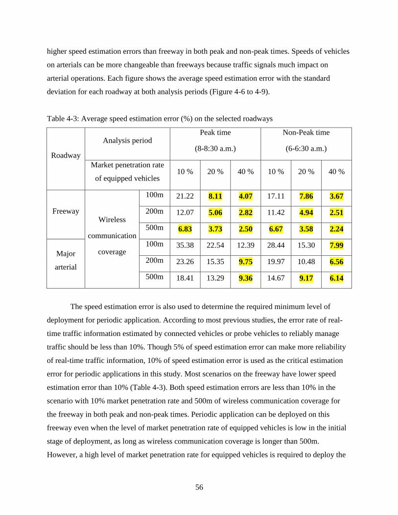
56

higher speed estimation errors than freeway in both peak and non-peak times. Speeds of vehicles

on arterials can be more changeable than freeways because traffic signals much impact on

arterial operations. Each figure shows the average speed estimation error with the standard

deviation for each roadway at both analysis periods (Figure 4-6 to 4-9).

Table 4-3: Average speed estimation error (%) on the selected roadways

Roadway

Analysis period Peak time

(8-8:30 a.m.)

Non-Peak time

(6-6:30 a.m.)



Freeway Wireless

communication

coverage

100m 21.22 8.11 4.07 17.11 7.86 3.67

200m 12.07 5.06 2.82 11.42 4.94 2.51

500m 6.83 3.73 2.50 6.67 3.58 2.24

Major

arterial

100m 35.38 22.54 12.39 28.44 15.30 7.99

200m 23.26 15.35 9.75 19.97 10.48 6.56

500m 18.41 13.29 9.36 14.67 9.17 6.14

The speed estimation error is also used to determine the required minimum level of

deployment for periodic application. According to most previous studies, the error rate of real-

time traffic information estimated by connected vehicles or probe vehicles to reliably manage

traffic should be less than 10%. Though 5% of speed estimation error can make more reliability

of real-time traffic information, 10% of speed estimation error is used as the critical estimation

error for periodic applications in this study. Most scenarios on the freeway have lower speed

estimation error than 10% (Table 4-3). Both speed estimation errors are less than 10% in the

scenario with 10% market penetration rate and 500m of wireless communication coverage for

the freeway in both peak and non-peak times. Periodic application can be deployed on this

freeway even when the level of market penetration rate of equipped vehicles is low in the initial

stage of deployment, as long as wireless communication coverage is longer than 500m.

However, a high level of market penetration rate for equipped vehicles is required to deploy the

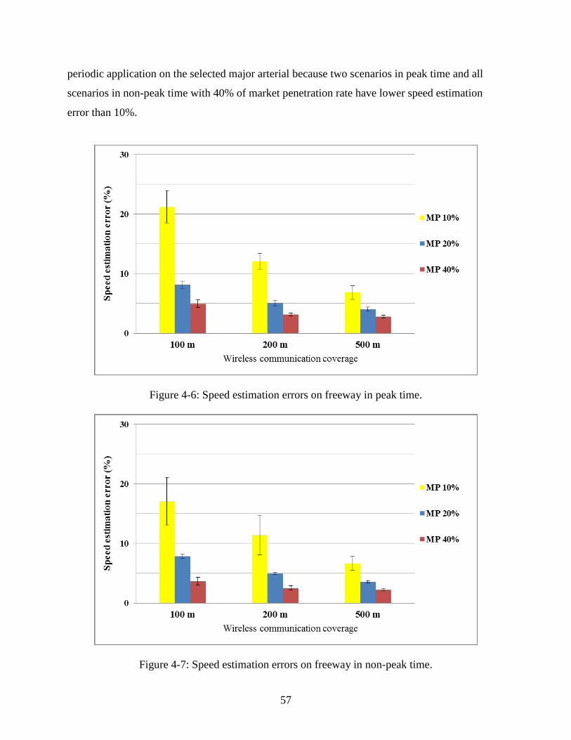
57

periodic application on the selected major arterial because two scenarios in peak time and all

scenarios in non-peak time with 40% of market penetration rate have lower speed estimation

error than 10%.

Figure 4-6: Speed estimation errors on freeway in peak time.

Figure 4-7: Speed estimation errors on freeway in non-peak time.

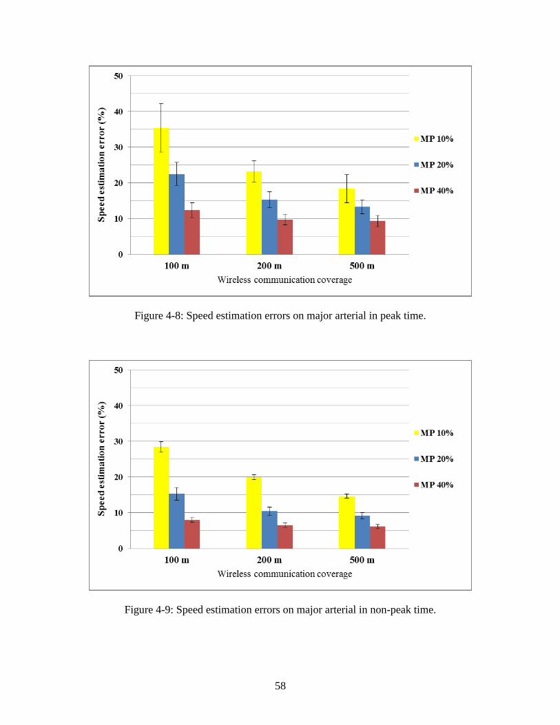
58

Figure 4-8: Speed estimation errors on major arterial in peak time.

Figure 4-9: Speed estimation errors on major arterial in non-peak time.

59

Section 4.7 Findings

This paper investigates the performance of V2V applications and determines the required

minimum level of deployment for V2V applications in an urban network. The distance of

information propagation and speed estimation error are used to measure the performance of

event-driven and periodic applications with different market penetration rates of equipped

vehicles and wireless communication coverage in both morning peak and non-peak times. As the

market penetration rate and wireless communication coverage increase, the distance of

information propagation increases while speed estimation error decreases in our study area. For

event-driven application, wireless communication coverage is the major factor because it has a

greater influence on the distance of information propagation. For periodic application, however,

the market penetration rate of equipped vehicles has more impact on performance than the

wireless communication coverage, because the speed estimation error more decreases as the

market penetration rate increases. The performance of event-driven improves in the higher traffic

density conditions of peak time while the performance of periodic application improves in the

lower traffic density conditions of non-peak time. The required minimum level of deployment

for each application is determined for various scenarios. These study findings will be useful for

deployments of connected vehicle applications. Notably, event-driven applications can even be

reliably deployed in the initial stage of deployment despite the low level of market penetration,

as long as sufficient wireless communication coverage is provided.

Future works will consider more factors impacting the performance of connected vehicle

applications because the performance of event-driven vehicle application can be varied with

other parameters, such as road networks, traffic pattern, location of event, and event duration.

Wireless communication signal interferences such as packet loss or delay also will be considered

in future works. The speed (or travel time) estimation error will be measured for the lower

functional class of roadways like minor arterial or collector during several time periods. Other

measurements for the performance of connected vehicle application can be investigated with the

same methodology.

60

Section 4.8 Acknowledgments

This research was supported by the Mid-Atlantic Universities Transportation Center (MAUTC).

This paper was peer-reviewed by TRB and presented at the TRB Annual Meeting, Washington,

D.C., January 2015.


Most references used in Chapter 4 are listed in Chapter 2 (LITERATURE REVIEW). Only new

references are listed in this section.

1. A.G. Hobeika, Taehyoung Kim, Heejin Jung, and B.Van Arem. Area Coverage Provided by

Vehicle to Vehicle Communication in an Urban Network. Presented at Conference on Agent

Based Modeling in Transportation Planning and Operations, Blacksburg, USA, Oct. 2013.

2. A.G. Hobeika et.al. TRANSIMS – The Microsimulation Module, A formal report submitted to

FHWA, Washington, D.C., 2000. (Placed on the web by FHWA, 2013)

3. Kwang-Sub Lee and A. G. Hobeika. Application of Dynamic Value Pricing Through

Enhancements to TRANSIMS. In Transportation Research Record: Journal of the



4. K.S. Lee, A.G. Hobeika, H.B. Zhang, and H.J. Jung. Travelers’ response to value pricing:

Application of departure time choices to TRANSIMS. Journal of Transportation Engineering,

Vol. 136, No. 9, 2010, pp. 811-817.

5. TRANSIMS manual: Network Data Tables.

http://transims.googlecode.com/svn/v4/trunk/documentation/usermanuals/Network%20Data%20

Tables%20v4.0.pdf. Accessed July 1, 2014.

6. ITS Standards Fact Sheets. ASTM E2213-03 - Standard Specification for Telecommunications

and Information Exchange Between Roadside and Vehicle Systems - 5 GHz Band Dedicated

Short Range Communications (DSRC) Medium Access Control (MAC) and Physical Layer

(PHY) Specifications. http://www.standards.its.dot.gov/Factsheets/Factsheet/66. Accessed

July 1, 2014.

61

7. ITS Standards Fact Sheets. IEEE 1609 - Family of Standards for Wireless Access in Vehicular

Environments (WAVE). http://www.standards.its.dot.gov/Factsheets/Factsheet/80. Accessed

July 1, 2014.



Penetration. In Transportation Research Record: Journal of the Transportation Research Board,

No. 2000, Transportation Research Board of the National Academies, Washington, D.C., 2007,

pp. 121–127.

62

Chapter 5 CONCLUSIONS

Section 5.1 Conclusions

This study represents connected vehicle environment in TRANSIMS to assess the performance

of V2V communication applications in the realistic urban network. The communication duration

rate and spatial-temporal dispersion of connected vehicles are investigated to evaluate the

capability of V2V communication based on the market penetration rate of equipped vehicles and

wireless communication coverage in the whole study area. The communication duration rate of

connected vehicles is more sensitive to the wireless communication coverage than the market

penetration rate. Equipped vehicles are able to keep the status of valid communicated vehicle at

least during 87% of the time stayed in the network when the market penetration rate is 10%.

The area coverage level is used to assess the spatial-temporal dispersion of connected

vehicles for two study areas; the Whole Network and the Selected Links cases. 12.27% of links

are covered by valid connected vehicles in the Whole Network case when the market penetration

rate is 40% and wireless communication coverage is 500m. The market penetration rate of

equipped vehicles has a greater influence on spatial-temporal dispersion of connected vehicles.

The Selected Links case has higher average area coverage level than the Whole Network case

because a higher percentage of equipped vehicles are on the selected links. The area coverage

varies by time of day and is sensitive to the density of traffic and to the aggregation level.

The distance of incident information propagation and speed estimation error are used to

measure the performance of event-driven and periodic applications based on different market

penetration rates of equipped vehicles and wireless communication coverage in both morning

peak and non-peak times. Both distance of information propagation and speed estimation error

are improved in our study area as the market penetration rate and wireless communication

coverage increase. The wireless communication coverage is the major factor for event-driven

application because it has a greater influence on the distance of information propagation than the

market penetration rate. In case of periodic application, however, the market penetration rate of

equipped vehicles has more impact on its performance than the wireless communication

coverage, because the speed estimation error more decreases as the market penetration rate

increases. The performance of event-driven improves in the higher traffic density conditions of

63

peak time while the performance of periodic application improves in the lower traffic density

conditions of non-peak time.

The required minimum levels of deployment for each application are determined for each

scenario. These study findings will be useful for making decisions about investments on

deployment of connected vehicle applications to improve the current transportation systems.

Notably, event-driven applications can be reliably deployed in the initial stage of deployment

despite the low level of market penetration of equipped vehicles, as long as sufficient wireless

communication coverage is provided.

Section 5.2 Future research

Future research will consider more different factors impacting the performance and required

minimum level of deployment for connected vehicle applications because the performance of

event-driven vehicle application can be varied with other parameters such as road networks,

traffic pattern, location of event, and event duration. The performance of periodic vehicle

application will be changed according to various parameters. The estimation error of real-time

traffic information will be measured for the lower functional class of roadways like minor

arterial or collector during several different time periods.

Though wireless communication signal interference is one of major factors to determine

the performance of connected vehicle application, this study assumed that there are no wireless

communication signal interferences in our simulation network. Wireless communication signal

interferences such as packet loss or delay also should be considered in future research to

represent the real connected vehicle environment. Our developed simulation model can be

integrated with the network simulation software (like NS-2) for wireless communication

features.

The real-time traffic information from connected vehicle applications can impact on

drivers’ travel pattern. Travelers can change their travel routes to avoid congested routes or make

green transportation choices by real-time traffic information. The changed network performance

can be considered as one of measurements for the performance of connected vehicle application.

Other measurements for the performance of connected vehicle application can be investigated

64

with the same methodology used in this study. Environmental impact such as fuel consumption

and emission can be used to do it.

65

Chapter 6 APPENDICES

Appendix A: Example of snapshot file with 20% of penetration rate of equipped vehicles

VEHICLE TIME LINK DIR LANE OFFSET SPEED ACCEL VEH_TYPE DRIVER PASSENGERS X_COORD Y_COORD Z_COORD BEARING

401002 6:00:00 3948 0 1 7.5 15 0 4 1 16 315218.2 4300202.4 0 163

404002 6:00:00 2359 1 1 90 7.5 -15 4 4 7 322634.1 4297065.2 0 100

413002 6:00:00 4235 0 1 30 15 0 4 13 0 319879.4 4301272.3 0 262

402002 6:00:00 654 0 1 15 0 0 4 2 35 321166.1 4297284.9 0 249

407002 6:00:00 1240 1 3 67.5 22.5 0 4 7 52 314771.8 4297524 0 192

410002 6:00:00 550 1 1 7.5 0 0 4 10 2 322500.5 4298629.7 0 99

6331 6:00:00 3066 0 2 300 30 7.5 1 633101 0 322545.5 4300226.3 0 343

76433 6:00:00 1223 0 2 472.5 30 0 1 7643301 0 322627.3 4299761.4 0 2

76460 6:00:00 1130 1 1 22.1 7.5 7.5 1 7646001 0 322561 4298974.1 0 84

76205 6:00:00 1223 0 2 427.5 22.5 -7.5 1 7620501 0 322625.7 4299716.7 0 2

9205 6:00:00 3066 0 3 52.5 30 0 1 920501 0 322618.4 4299993.9 0 343

414002 6:00:00 2602 0 1 120 0 0 4 14 1 322522.2 4296963 0 191

78299 6:00:00 567 0 2 105 0 0 1 7829901 0 322419.4 4297990.8 0 10

7929 6:00:00 3066 0 2 52.5 30 0 1 792901 0 322618.4 4299993.9 0 343

76371 6:00:00 567 0 2 90 0 0 1 7637101 0 322416.7 4297976.1 0 10

76191 6:00:00 2633 1 2 94 7.5 7.5 1 7619101 0 322111.8 4297941.6 0 101

61329 6:00:00 567 0 1 105 0 0 1 6132901 0 322419.4 4297990.8 0 10

70751 6:00:00 1132 1 1 15 0 0 1 7075101 0 322532 4298971.5 0 87

174308 6:00:00 6049 1 5 247.5 37.5 0 11 17430801 2 319770.7 4302168 0 35

247949 6:00:00 2570 1 1 67.5 15 0 1 24794901 0 322178 4296362.6 0 100

18839 6:00:00 2154 1 1 30 22.5 0 1 1883901 0 321956.8 4300204.4 0 355

70581 6:00:00 1132 1 1 7.5 0 0 1 7058101 0 322524.6 4298971 0 87

5131 6:00:00 749 1 2 97.5 0 0 1 513101 0 321260.5 4297059.6 0 102

176903 6:00:00 1223 0 3 630 22.5 -7.5 11 17690301 2 322632.9 4299917.8 0 2

265137 6:00:00 567 0 1 120 0 0 1 26513701 0 322422 4298005.6 0 10

33702 6:00:00 6049 1 5 45 37.5 0 1 3370201 0 319655.5 4302001.5 0 35

70816 6:00:00 1133 1 1 30 0 0 1 7081601 0 322510.1 4298970 0 85

33362 6:00:00 13 0 7 300 37.5 0 1 3336201 0 319589.8 4301903 0 33

61608 6:00:00 586 0 1 133 22.5 0 1 6160801 0 322086.7 4296244.2 0 191

81829 6:00:00 1133 1 1 22.5 0 0 1 8182901 0 322502.6 4298969.4 0 85

15354 6:00:00 3066 0 3 120 30 7.5 1 1535401 0 322598.6 4300057.3 0 343

18982 6:00:00 2026 0 4 127 7.5 7.5 1 1898201 0 322159.6 4298192.6 0 11

3954 6:00:00 6049 1 6 67.5 30 -7.5 1 395401 0 319668.3 4302020 0 35

59091 6:00:00 2154 1 1 60 22.5 0 1 5909101 0 321954.4 4300234.3 0 355

2093 6:00:00 13 0 6 127.5 37.5 0 1 209301 0 319497.7 4301761.4 0 33

29436 6:00:00 4902 1 2 225 0 0 1 2943601 0 317102.9 4301306.1 0 325

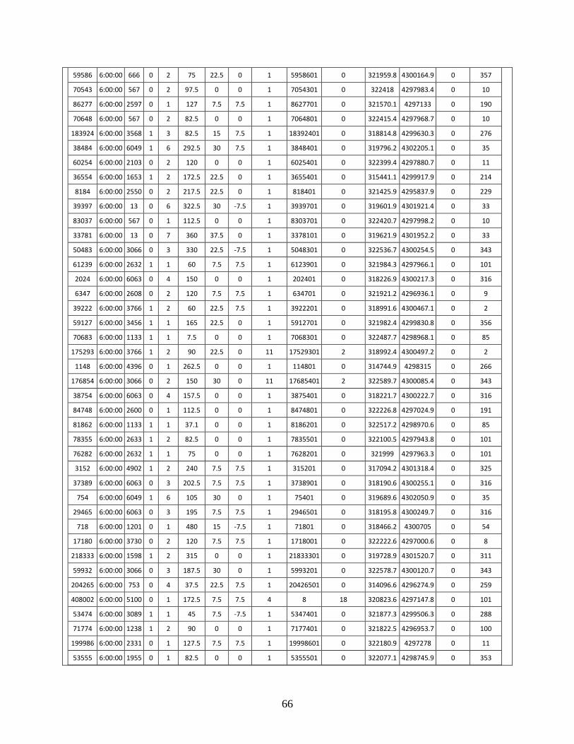
66

59586 6:00:00 666 0 2 75 22.5 0 1 5958601 0 321959.8 4300164.9 0 357

70543 6:00:00 567 0 2 97.5 0 0 1 7054301 0 322418 4297983.4 0 10

86277 6:00:00 2597 0 1 127 7.5 7.5 1 8627701 0 321570.1 4297133 0 190

70648 6:00:00 567 0 2 82.5 0 0 1 7064801 0 322415.4 4297968.7 0 10

183924 6:00:00 3568 1 3 82.5 15 7.5 1 18392401 0 318814.8 4299630.3 0 276

38484 6:00:00 6049 1 6 292.5 30 7.5 1 3848401 0 319796.2 4302205.1 0 35

60254 6:00:00 2103 0 2 120 0 0 1 6025401 0 322399.4 4297880.7 0 11

36554 6:00:00 1653 1 2 172.5 22.5 0 1 3655401 0 315441.1 4299917.9 0 214

8184 6:00:00 2550 0 2 217.5 22.5 0 1 818401 0 321425.9 4295837.9 0 229

39397 6:00:00 13 0 6 322.5 30 -7.5 1 3939701 0 319601.9 4301921.4 0 33

83037 6:00:00 567 0 1 112.5 0 0 1 8303701 0 322420.7 4297998.2 0 10

33781 6:00:00 13 0 7 360 37.5 0 1 3378101 0 319621.9 4301952.2 0 33

50483 6:00:00 3066 0 3 330 22.5 -7.5 1 5048301 0 322536.7 4300254.5 0 343

61239 6:00:00 2632 1 1 60 7.5 7.5 1 6123901 0 321984.3 4297966.1 0 101

2024 6:00:00 6063 0 4 150 0 0 1 202401 0 318226.9 4300217.3 0 316

6347 6:00:00 2608 0 2 120 7.5 7.5 1 634701 0 321921.2 4296936.1 0 9

39222 6:00:00 3766 1 2 60 22.5 7.5 1 3922201 0 318991.6 4300467.1 0 2

59127 6:00:00 3456 1 1 165 22.5 0 1 5912701 0 321982.4 4299830.8 0 356

70683 6:00:00 1133 1 1 7.5 0 0 1 7068301 0 322487.7 4298968.1 0 85

175293 6:00:00 3766 1 2 90 22.5 0 11 17529301 2 318992.4 4300497.2 0 2

1148 6:00:00 4396 0 1 262.5 0 0 1 114801 0 314744.9 4298315 0 266

176854 6:00:00 3066 0 2 150 30 0 11 17685401 2 322589.7 4300085.4 0 343

38754 6:00:00 6063 0 4 157.5 0 0 1 3875401 0 318221.7 4300222.7 0 316

84748 6:00:00 2600 0 1 112.5 0 0 1 8474801 0 322226.8 4297024.9 0 191

81862 6:00:00 1133 1 1 37.1 0 0 1 8186201 0 322517.2 4298970.6 0 85

78355 6:00:00 2633 1 2 82.5 0 0 1 7835501 0 322100.5 4297943.8 0 101

76282 6:00:00 2632 1 1 75 0 0 1 7628201 0 321999 4297963.3 0 101

3152 6:00:00 4902 1 2 240 7.5 7.5 1 315201 0 317094.2 4301318.4 0 325

37389 6:00:00 6063 0 3 202.5 7.5 7.5 1 3738901 0 318190.6 4300255.1 0 316

754 6:00:00 6049 1 6 105 30 0 1 75401 0 319689.6 4302050.9 0 35

29465 6:00:00 6063 0 3 195 7.5 7.5 1 2946501 0 318195.8 4300249.7 0 316

718 6:00:00 1201 0 1 480 15 -7.5 1 71801 0 318466.2 4300705 0 54

17180 6:00:00 3730 0 2 120 7.5 7.5 1 1718001 0 322222.6 4297000.6 0 8

218333 6:00:00 1598 1 2 315 0 0 1 21833301 0 319728.9 4301520.7 0 311

59932 6:00:00 3066 0 3 187.5 30 0 1 5993201 0 322578.7 4300120.7 0 343

204265 6:00:00 753 0 4 37.5 22.5 7.5 1 20426501 0 314096.6 4296274.9 0 259

408002 6:00:00 5100 0 1 172.5 7.5 7.5 4 8 18 320823.6 4297147.8 0 101

53474 6:00:00 3089 1 1 45 7.5 -7.5 1 5347401 0 321877.3 4299506.3 0 288

71774 6:00:00 1238 1 2 90 0 0 1 7177401 0 321822.5 4296953.7 0 100

199986 6:00:00 2331 0 1 127.5 7.5 7.5 1 19998601 0 322180.9 4297278 0 11

53555 6:00:00 1955 0 1 82.5 0 0 1 5355501 0 322077.1 4298745.9 0 353

67

174488 6:00:00 567 0 1 97.5 0 0 11 17448801 2 322418 4297983.4 0 10

33812 6:00:00 6063 0 4 127.5 7.5 -7.5 1 3381201 0 318242.4 4300201.1 0 316

33636 6:00:00 4873 0 5 15 22.5 7.5 1 3363601 0 319325.4 4301474.4 0 30

59437 6:00:00 1955 0 2 67.5 0 0 1 5943701 0 322078.9 4298731.1 0 353

175194 6:00:00 5000 0 2 37.5 15 0 11 17519401 2 316341.3 4300364 0 324

70575 6:00:00 2628 1 1 60 7.5 -7.5 1 7057501 0 321890.7 4297983.7 0 101

32693 6:00:00 6049 1 6 30 30 -7.5 1 3269301 0 319647 4301989.2 0 35

57994 6:00:00 4734 0 3 82.5 22.5 0 1 5799401 0 315905.2 4301277.4 0 23

50430 6:00:00 1955 0 2 60 0 0 1 5043001 0 322079.7 4298723.7 0 353

77932 6:00:00 2852 0 2 45 0 0 1 7793201 0 321173.6 4297301.9 0 151

1814 6:00:00 6063 0 4 142.5 0 0 1 181401 0 318232.1 4300211.9 0 316

11402 6:00:00 511 0 1 195 15 7.5 1 1140201 0 321634.8 4296155.1 0 233

176659 6:00:00 1955 0 2 75 0 0 11 17665901 2 322078 4298738.5 0 353

60578 6:00:00 567 0 2 120 0 0 1 6057801 0 322422 4298005.6 0 10

32392 6:00:00 5000 0 2 105 22.5 0 1 3239201 0 316301.3 4300418.1 0 324

39440 6:00:00 6063 0 4 195 7.5 7.5 1 3944001 0 318195.8 4300249.7 0 316

26149 6:00:00 5000 0 1 225 7.5 7.5 1 2614901 0 316230.2 4300514.4 0 324

38749 6:00:00 6063 0 4 135 0 -7.5 1 3874901 0 318237.2 4300206.5 0 316

18053 6:00:00 4605 1 2 210 7.5 0 1 1805301 0 322034.5 4298793.2 0 130

39367 6:00:00 6049 1 6 247.5 15 -22.5 1 3936701 0 319770.7 4302168 0 35

50825 6:00:00 2069 0 1 22.5 7.5 -7.5 1 5082501 0 322692.8 4297856.9 0 11

78283 6:00:00 4876 0 3 82.5 15 -7.5 1 7828301 0 321858.9 4301394.8 0 355

50285 6:00:00 1598 1 2 277.5 0 0 1 5028501 0 319754 4301499 0 311

175241 6:00:00 3766 1 2 30 15 -7.5 11 17524101 2 318990.7 4300437.1 0 2

38849 6:00:00 3764 1 2 52.5 22.5 0 1 3884901 0 319008.7 4300560.2 0 18

33302 6:00:00 3764 1 2 90 22.5 0 1 3330201 0 319020 4300595.9 0 18

4180 6:00:00 6049 1 6 195 37.5 0 1 418001 0 319740.8 4302124.9 0 35

224335 6:00:00 2042 0 1 82.5 15 0 1 22433501 0 322728 4298041.8 0 11

288 6:00:00 3568 1 2 52.5 7.5 0 1 28801 0 318844.6 4299626.9 0 276

1358 6:00:00 6049 1 6 150 37.5 7.5 1 135801 0 319715.2 4302087.9 0 35

10580 6:00:00 2104 1 2 90 0 0 1 1058001 0 322364.8 4297765 0 100

84741 6:00:00 2600 0 2 127 7.5 7.5 1 8474101 0 322224 4297010.6 0 191

50789 6:00:00 2629 0 2 45 15 0 1 5078901 0 322815.5 4297988 0 11

60526 6:00:00 3733 1 1 127.5 7.5 7.5 1 6052601 0 322279.3 4297256.8 0 14

176646 6:00:00 4240 1 1 165 15 0 11 17664601 2 319566.6 4301103.4 0 7

29240 6:00:00 5000 0 2 217.5 0 0 1 2924001 0 316234.6 4300508.4 0 324

176074 6:00:00 2629 0 2 75 15 0 11 17607401 2 322821.2 4298017.5 0 11

76413 6:00:00 4776 1 1 232.5 0 0 1 7641301 0 321666.5 4298010.1 0 117

47608 6:00:00 111 0 2 45 22.5 0 1 4760801 0 315945.9 4301297.9 0 64

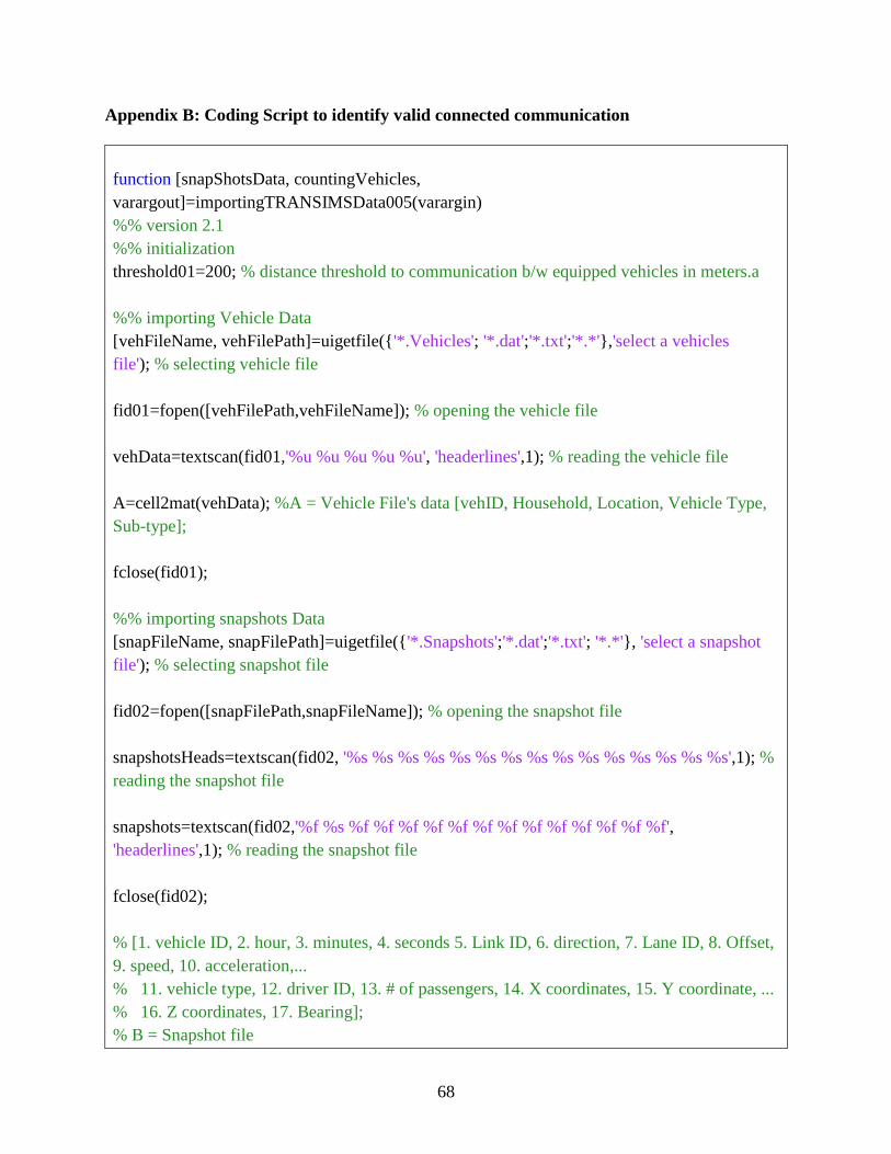
68

Appendix B: Coding Script to identify valid connected communication

function [snapShotsData, countingVehicles,

varargout]=importingTRANSIMSData005(varargin)

%% version 2.1

%% initialization

threshold01=200; % distance threshold to communication b/w equipped vehicles in meters.a

%% importing Vehicle Data

[vehFileName, vehFilePath]=uigetfile({'*.Vehicles'; '*.dat';'*.txt';'*.*'},'select a vehicles

file'); % selecting vehicle file

fid01=fopen([vehFilePath,vehFileName]); % opening the vehicle file

vehData=textscan(fid01,'%u %u %u %u %u', 'headerlines',1); % reading the vehicle file

A=cell2mat(vehData); %A = Vehicle File's data [vehID, Household, Location, Vehicle Type,

Sub-type];

fclose(fid01);

%% importing snapshots Data

[snapFileName, snapFilePath]=uigetfile({'*.Snapshots';'*.dat';'*.txt'; '*.*'}, 'select a snapshot

file'); % selecting snapshot file

fid02=fopen([snapFilePath,snapFileName]); % opening the snapshot file

snapshotsHeads=textscan(fid02, '%s %s %s %s %s %s %s %s %s %s %s %s %s %s %s',1); %

reading the snapshot file

snapshots=textscan(fid02,'%f %s %f %f %f %f %f %f %f %f %f %f %f %f %f',

'headerlines',1); % reading the snapshot file

fclose(fid02);

% [1. vehicle ID, 2. hour, 3. minutes, 4. seconds 5. Link ID, 6. direction, 7. Lane ID, 8. Offset,

9. speed, 10. acceleration,...

% 11. vehicle type, 12. driver ID, 13. # of passengers, 14. X coordinates, 15. Y coordinate, ...

% 16. Z coordinates, 17. Bearing];

% B = Snapshot file

69

T=snapshots{1,2};

B=snapshots;

B(2)=[];

times=convertingTimeData(T);% convert a string cell array of time to N-by-3 numeric array

snapshots=cell2mat(B); % convert a cell array to numeric array

snapShotsData=[snapshots(:,1), times, snapshots(:,2:end)];

%% separating equipped vehicles and unequipped vehicles

% rule: equipped vehicle is a vehicle that is 1 of vehicle type and 2 of

% sub-vehicle type.

indx01=A(:,4)==1;

indx02=A(:,5)==2;

indx03=find(indx01.*indx02); % equipped vehicles

if ~isempty(indx03)

equippedVehID=A(indx03,1);

else

equippedVehID=[];

end

%% importing study Links and filtering

if nargin>0

studyLinkIds=varargin{1};

indx=find(ismember(snapShotsData(:,5),studyLinkIds));

if ~isempty(indx)

snapShotsData=snapShotsData(indx,:);

else

snapShotsData=[];

end

70

end

%% categorizing vehicles

% Step 1 dividing by time period

times=snapShotsData(:,2)*10000+snapShotsData(:,3)*100+snapShotsData(:,4);

%distances=NaN*ones(size(times));

timeLog=unique(times);

numTimeLogs=size(timeLog,1);

dvdTimeDB.timeLogs=timeLog;

dvdTimeDB.data=cell(numTimeLogs,4);

countingVehicles=zeros(numTimeLogs,5);

for k=1:numTimeLogs

timelog=timeLog(k);

indxTime=find(times==timelog);

if ~isempty(indxTime) % at this time, there are one or more vehicles observed

dvdTimeDB.data{k,1}=snapShotsData(indxTime,:);

countingVehicles(k,1)=numel(indxTime); % total Number of vehicles

if ~isempty(equippedVehID) % There are one or more equipped vehicles on entire

observed time period.

indxequppdvehs=find(ismember(dvdTimeDB.data{k,1}(:,1),equippedVehID));

if ~isempty(indxequppdvehs) % There are one or more equipped vehicles (==3) at this

time

dvdTimeDB.data{k,1}(indxequppdvehs,11)=3;

snapShotsData(indxTime(indxequppdvehs),11)=3;

countingVehicles(k,3)=numel(indxequppdvehs); % total Number of equipped

vehicles

countingVehicles(k,2)=countingVehicles(k,1)-countingVehicles(k,3); % total

Number of non-equipped vehicles

X=dvdTimeDB.data{k,1}(indxequppdvehs,[14 15]); % X & Y coordinates

dvdTimeDB.data{k,3}=dvdTimeDB.data{k,1}(indxequppdvehs,[1 5 6 7 14 15]); %

[vehicle ID, Link ID, direction, Lane ID, X coordinates, Y coordinate]

numEqpdveh=size(indxequppdvehs,1);

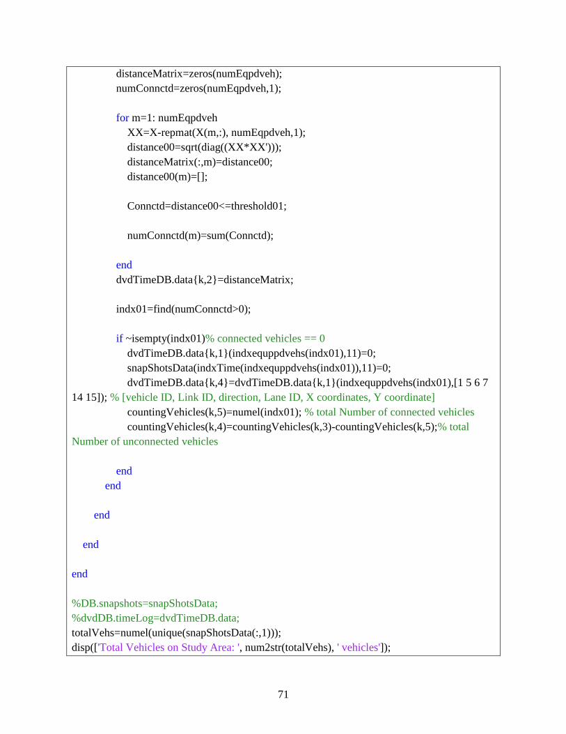
71

distanceMatrix=zeros(numEqpdveh);

numConnctd=zeros(numEqpdveh,1);

for m=1: numEqpdveh

XX=X-repmat(X(m,:), numEqpdveh,1);

distance00=sqrt(diag((XX*XX')));

distanceMatrix(:,m)=distance00;

distance00(m)=[];

Connctd=distance00<=threshold01;

numConnctd(m)=sum(Connctd);

end

dvdTimeDB.data{k,2}=distanceMatrix;

indx01=find(numConnctd>0);

if ~isempty(indx01)% connected vehicles == 0

dvdTimeDB.data{k,1}(indxequppdvehs(indx01),11)=0;

snapShotsData(indxTime(indxequppdvehs(indx01)),11)=0;

dvdTimeDB.data{k,4}=dvdTimeDB.data{k,1}(indxequppdvehs(indx01),[1 5 6 7

14 15]); % [vehicle ID, Link ID, direction, Lane ID, X coordinates, Y coordinate]

countingVehicles(k,5)=numel(indx01); % total Number of connected vehicles

countingVehicles(k,4)=countingVehicles(k,3)-countingVehicles(k,5);% total

Number of unconnected vehicles

end

end

end

end

end

%DB.snapshots=snapShotsData;

%dvdDB.timeLog=dvdTimeDB.data;

totalVehs=numel(unique(snapShotsData(:,1)));

disp(['Total Vehicles on Study Area: ', num2str(totalVehs), ' vehicles']);

72

indx01=find((snapShotsData(:,11)==3)+(snapShotsData(:,11)==0));

indx02=find(snapShotsData(:,11)==0);

if ~isempty(indx01)

totalEqpVehs=numel(unique(snapShotsData(indx01,1)));

else

totalEqpVehs=0;

end

if ~isempty(indx02)

totalConnectedVehs=numel(unique(snapShotsData(indx02,1)));

else

totalConnectedVehs=0;

end

disp(['Total Non-Equipped Vehicles on Study Area: ', num2str(totalVehs-totalEqpVehs), '

vehicles']);

disp(['Total Equipped Vehicles on Study Area: ', num2str(totalEqpVehs), ' vehicles']);

disp(['Total unconnected Vehicles on Study Area: ', num2str(totalEqpVehs-

totalConnectedVehs), ' vehicles']);

disp(['Total connected Vehicles on Study Area: ', num2str(totalConnectedVehs), ' vehicles']);

countingVehicles=[[dvdTimeDB.timeLogs;0],[countingVehicles;[totalVehs, totalVehs-

totalEqpVehs,...

totalEqpVehs, totalEqpVehs-totalConnectedVehs, totalConnectedVehs]]];

if nargout>2

varargout{1}=snapshotsHeads;

if nargout>3

varargout{2}=dvdTimeDB;

end

73

end

%% Exporting snapshots Data

ExportingSnapshotsData(snapshotsHeads,snapShotsData);

74

Appendix C: Coding Script to measure the communication duration rate

function [CDR, varargout]=KTH_computeComDurRate(setSimObj)

%% I. Importing Vehicle Data

disp('>>> Importing Data ');

disp('>>> >>> Importing the Vehicle Data...');

disp(' ');

disp(' ');

fidV=fopen([setSimObj.fileManger.vehicle.path,setSimObj.fileManger.vehicle.fileName]);

disp('>>> >>> Cimplete Importing the Vehicle Data...');

disp(' ');

disp(' ');

%% data of Vehicle File: [1. Vehicle_ID, 2. HHOLD, 3. Location, 4. Type, 5. Subtype]

if ~isempty(setSimObj.fileManger.vehicle.N)

vehData=textscan(fidV,setSimObj.fileManger.vehicle.format,

setSimObj.fileManger.vehicle.N,'headerlines',setSimObj.fileManger.vehicle.headlines);

else


'headerlines',setSimObj.fileManger.vehicle.headlines);

end

fclose(fidV);

%% vehData=[1. Vehicle_ID, 2. Type, 3. Subtype]

vehData=cell2mat(vehData);

disp('>>> >>> Cimplete Importing the Vehicle Data...');

disp(' ');

disp(' ');

%% II. Classification Vehicles into Two Groups:

%% Non-equipped Vehicles and Equipped Vehicles Groups (Vehicle Type=3).

%% Based on the Vehicle Data

%% Rule for Equipped Vehicles: vehicle type and sub-vehicle type are 1 and 2, respectively.

%% That is, vehData(:,2)==1 && vehData(:,3)==2

disp('>>> Classification ');

75

disp('>>> >>> Classification all Vehicles into two groups: nonequipped and equipped

vehicles'' groups...');

disp(' ');

disp(' ');

indxNonEq=find((vehData(:,2)~=1)+(vehData(:,3)~=2));

indxEq=find((vehData(:,2)==1).*(vehData(:,3)==2));

vehicles.count.Total=numel(vehData(:,1));

if ~isempty(indxNonEq)

vehicles.IDs.NonEq=sort(vehData(indxNonEq,1));

vehicles.count.NonEq=numel(indxNonEq);

else

vehicles.IDs.NonEq=[];

vehicles.count.NonEq=0;

end

if ~isempty(indxEq)

vehicles.IDs.Eq=sort(vehData(indxEq,1));

vehicles.count.Eq=numel(indxEq);

else

vehicles.IDs.Eq=[];

vehicles.count.Eq=0;

end

disp('>>> >>> Complete the Classification');

disp(' ');

disp(' ');

%% II. Compute Communication Duration Rate

CDR=[vehicles.IDs.Eq, zeros(numel(vehicles.IDs.Eq),4)];

IDX=repmat(vehicles.IDs.Eq, 1,2)*1000+repmat([0 3], numel(vehicles.IDs.Eq),1);

maxN=1000000;

76

[setSimObj.fileManger.snapshot.fileName,

setSimObj.fileManger.snapshot.path]=uigetfile({'*.Snapshots';'*.dat';'*.txt'; '*.*'}, 'select a

snapshot file');

fidS=fopen([setSimObj.fileManger.snapshot.path,setSimObj.fileManger.snapshot.fileName]);

data=textscan(fidS, '%f %*s %*f %*f %*f %*f %*f %*f %f %*f %*f %*f %*f %*f %*f',

maxN, 'headerlines', 1);

data=cell2mat(data);

data=data(:,1)*1000+data(:,2);

CON=countingElements0001(IDX(:,1), data);

NonCon=countingElements0001(IDX(:,2), data);

CDR(:,[3 4])=[CDR(:,3)+CON(:,2), CDR(:,4)+NonCon(:,2)];

while ~isempty(data)

%% data of Snapshots File: [1.Vehicle_ID, 2. Time, 3. Link_ID 4. DIR,

%% 5.Lane, 6. Offset, 7. Speed, 8. Accel, 9. Veh_Type, 10. Driver,

%% 11. Passenger 12. X_Coordinate, 13. Y_Coordinate, 14. Y_Coordinate, 15.

%% Bearing]

data=textscan(fidS, '%f %*s %*f %*f %*f %*f %*f %*f %f %*f %*f %*f %*f %*f %*f',

maxN, 'headerlines', 1);

if ~isempty(data{1,1})


data=data(:,1)*1000+data(:,2);

CON=countingElements0001(IDX(:,1), data);

NonCon=countingElements0001(IDX(:,2), data);

CDR(:,[3 4])=[CDR(:,3)+CON(:,2), CDR(:,4)+NonCon(:,2)];

else

77

data=[];

end

end

fclose(fidS);

CDR(:,2)=sum(CDR(:,[3 4]),2);

CDR(:,5)=CDR(:,3)./CDR(:,2)*100;

indx01=find(~isnan(CDR(:,5)));

if ~isempty(indx01)

figure(1)

subplot(2,1,1)

[n1, xout1]=hist(CDR(indx01,2), 100);

bar(xout1, n1, 'b')

title('Distribution of # of datasets of equipped vehicles');

xlabel('Bin of # of datasets');

ylabel('# of equipped vehicles');

grid on

subplot(2,1,2)

[n2, xout2]=hist(CDR(indx01,5), 100);

bar(xout2, n2, 'b')

title('Distribution of # of connection duration rates of datasets of equipped vehicles');

xlabel('Bin of connection duration rate (%)');

ylabel('# of equipped vehicles');

grid on

end

if nargout>=2

varargout{1}=[xout1; n1];

if nargout>=3

varargout{2}=[xout2; n2];

end

end

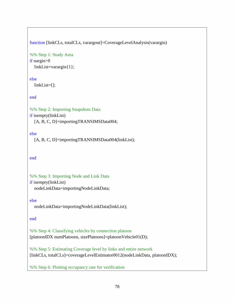
78

function [linkCLs, totalCLs, varargout]=CoverageLevelAnalysis(varargin)

%% Step 1: Study Area

if nargin>0

linkList=varargin{1};

else

linkList=[];

end

%% Step 2: Importing Snapshots Data

if isempty(linkList)

[A, B, C, D]=importingTRANSIMSData004;

else

[A, B, C, D]=importingTRANSIMSData004(linkList);

end

%% Step 3: Importing Node and Link Data

if isempty(linkList)

nodeLinkData=importingNodeLinkData;

else

nodeLinkData=importingNodeLinkData(linkList);

end

%% Step 4: Classifying vehicles by connection platoon

[platoonIDX numPlatoons, sizePlatoons]=platoonVehicle01(D);

%% Step 5: Estimating Coverage level by links and entire network

[linkCLs, totalCLs]=coverageLevelEstimator0012(nodeLinkData, platoonIDX);

%% Step 6: Plotting occupancy rate for verification

79

figure(1);

numNodes=size(nodeLinkData(:,3),1);

k=1;

X1=reshape(([nodeLinkData(:,[3 6]), NaN*ones(numNodes,1)])', [], 1) ;

Y1=reshape(([nodeLinkData(:,[4 7]), NaN*ones(numNodes,1)])', [], 1) ;

plot(X1,Y1, 'k-o');

figure;

times=(1:size(D.timeLogs,1))';

plot(times, totalCLs(:,1), 'r-', times, totalCLs(:,3), 'b-');

xlabel('timelog (minutes)');

ylabel('Occupancy rate (%)');

legend({'coverage level';'occupied link'});

grid on

if nargout>2

varargout{1}=platoonIDX;

if nargout>3

varargout{2}=numPlatoons;

if nargout>4

varargout{3}=sizePlatoons;

if nargout>5

varargout{4}=A; % data for snapshots file

if nargout>6

varargout{5}=B; % # of vehicles

if nargout>7

varargout{6}=C; % heads of snapshots file

if nargout>8

varargout{7}=D; % separated data by timelogs

end

80

end

end

end

end

end

end

81

Appendix D: Coding Script to measure the area coverage by connected vehicles

function [linkCLs, totalCLs]=coverageLevelEstimator0012(nodeLinkData, platoonsIDX)

%% version 1.2

%% coded by Heejin Jung

numTimelog=size(platoonsIDX,1);

%% Link Listing

linkIDs=nodeLinkData(:,1);

%numLinks=numel(linkIDs);

%% computing total Length

linkLengths=nodeLinkData(:,8);

totalLength=sum(linkLengths);

linkCLs=cell(size(platoonsIDX));

totalCLs=zeros(size(platoonsIDX,1),4);

%% computinh uncoverage length

for k=1:numTimelog

%% L

indiCLs=[linkIDs, zeros(size(linkIDs)), linkLengths,abs(nodeLinkData(:,6)-

nodeLinkData(:,3)), NaN*ones(size(linkIDs,1),3)]; %[ link ID, projected axis, link Length,

projected link length, total projected covered length, total covered length]

%% M

indxY=find(abs(nodeLinkData(:,6)-nodeLinkData(:,3))<abs(nodeLinkData(:,7)-

nodeLinkData(:,4)));

if ~isempty(indxY)

indiCLs(indxY,4)=abs(nodeLinkData(indxY,7)-nodeLinkData(indxY,4));

indiCLs(indxY,2)=1;

end

pData=platoonsIDX{k,1}; % [connected vehicle id, link id, x-coordinate, y-coordinate,

platoon id];

if ~isempty(pData) % if there is one or more connected vehicles

82

indx01=find(~ismember(linkIDs, unique(pData(:,2)))); % links without connected

vehicles

if ~isempty(indx01)

indiCLs(indx01,5)=0;

end

indx02=find(ismember(linkIDs, unique(pData(:,2)))); % links with one or more

connected vehicles

if ~isempty(indx02)

for m=indx02' % links

indicls=indiCLs(m,:);

pltoonsList=constructingPlatoonsList(indicls, pData, nodeLinkData);

indiCLs(m,5)=sum(pltoonsList(:,3)-pltoonsList(:,2));

end

end

%indiCLs=[ link ID, projected axis, link Length, projected link length, total projected

covered length, total covered length, coverage level]

indiCLs(:,6)=indiCLs(:,3).*indiCLs(:,5)./indiCLs(:,4);

indiCLs(:,7)=indiCLs(:,6)./indiCLs(:,3)*100;

linkCLs{k,1}=indiCLs;

totalCLs(k,1)=sum(indiCLs(:,6))/totalLength*100;

totalCLs(k,4)=sum(indiCLs(:,6));

indx01=find(indiCLs(:,6));

if ~isempty(indx01)

totalCLs(k,2)=numel(indx01);

end

else %% there is no platoons

83

linkCLs{k,1}=[];

totalCLs(k,1)=0;

totalCLs(k,2)=0;

totalCLs(k,4)=0;

end

end

totalCLs(:,3)=totalCLs(:,2)/size(nodeLinkData(:,1),1)*100;

84

Appendix E: Coding Script to measure the distance of information propagation

%% Building Simulation Setting Object (KTH_buildingSimSetObj003.m)

%% Set Research Scope

% Spatial scope

KTH_setVariable4ResearchArea002;

%% Set Thresholds

setSimObj.threshold.V2V_Range=100; % in meters

%% Set Scenarios

% [VEHICLE HHOLD LOCATION TYPE SUBTYPE]

setSimObj.disabledVeh.blockedLinkID=10;

setSimObj.disabledVeh.blockedDirection=1;

setSimObj.disabledVeh.blockedLane=2;

setSimObj.disabledVeh.offset=0;

setSimObj.disabledVeh.driverID=0;

setSimObj.disabledVeh.passenger=0;

setSimObj.disabledVeh.Types=[1 2]; % [Type subType] for Equipped vehicle, else

Nonequipped vehicle

setSimObj.disabledVeh.coordinates=[10,10]; % [x y z]; % update is required

setSimObj.disabledVeh.communicationDirection=1; %1: x to be increase, -1;

x to be decrease, 2: y to be increase, -2: y to be decrease

%% file Manger

% vehicle file

[setSimObj.fileManger.vehicle.fileName, setSimObj.fileManger.vehicle.path]=uigetfile

({'*.Vehicles'; '*.dat';'*.txt';'*.*'},'select a vehicles file'); % selecting vehicle file

setSimObj.fileManger.vehicle.format='%n %n %n %n %n';

setSimObj.fileManger.vehicle.N=[];

setSimObj.fileManger.vehicle.headlines=1;

% snapshots file

[setSimObj.fileManger.snapshot.fileName, setSimObj.fileManger.snapshot.path]=uigetfile

({'*.Snapshots';'*.dat';'*.txt'; '*.*'}, 'select a snapshot file'); % selecting snapshot file

setSimObj.fileManger.snapshot.format.headings='%s %s %s %s %s %s %s %s %s %s %s

%s %s %s %s';

85

setSimObj.fileManger.snapshot.format.data='%f %s %f %f %f %f %f %f %f %f %f %f %f

%f %f';

setSimObj.fileManger.snapshot.format.writing='%u\t%u\t%u\t%u\t%u\t%6.2f\t%4.2f\t%4.

2f\t%u\t%u\t%u\t%10.1f\t%10.1f\t%10.1f\t%u\n';

% snapshots file

setSimObj.fileManger.snapshot.path2=[uigetdir(setSimObj.fileManger.snapshot.path,

'select directory to save new sanpshots file.'), '\']; % selecting snapshot file

setSimObj.fileManger.snapshot.fileName2=['New_',

setSimObj.fileManger.snapshot.fileName];

setSimObj.fileManger.snapshot.format.headings2='%s \n';

setSimObj.fileManger.snapshot.format.data2.reading='%f %f %f %f %f %f %f %f %f %f %f

%f %f %f %f';

setSimObj.fileManger.snapshot.format.data2.writing='%u\t%u\t%u\t%u\t%u\t%6.2f\t%4.2f\t

%4.2f\t%u\t%u\t%u\t%10.1f\t%10.1f\t%10.1f\t%u\n';

if ~isdir([setSimObj.fileManger.snapshot.path,'dummies'])

mkdir(setSimObj.fileManger.snapshot.path(1:end-1), 'dummies' );

end

% Time scope


setSimObj.parameters.maxN=1000000;

data=textscan(fidS, '%*f %s %*f %*f %*f %*f %*f %*f %*f %*f %*f %*f %*f %*f %*f',

'headerlines', 1);

setSimObj.Scope.T=[];

while ~isempty(data{1,1})

A=setSimObj.Scope.T;

T=KTH_convertStrTime2hhmmss002(data{1,1}, ':');

setSimObj.Scope.T=unique([setSimObj.Scope.T;T]);

86

data=textscan(fidS, '%*f %s %*f %*f %*f %*f %*f %*f %*f %*f %*f %*f %*f %*f %*f',

setSimObj.parameters.maxN);

end

fclose(fidS);

setSimObj.Scope.Period=[setSimObj.Scope.T(1), setSimObj.Scope.T(end)];

%% dummy

setSimObj.fileManger.dummy.path=[setSimObj.fileManger.snapshot.path2, 'dummies\'];

setSimObj.fileManger.dummy.filename='dummy';

setSimObj.fileManger.dummy.extension='.dat';

setSimObj.fileManger.dummy.format.reading='%n %n %n %n %n %f %f %f %n %n %n %f

%f %f %n';

setSimObj.fileManger.dummy.format.writing='%u \t %u \t %u \t %u \t %u \t %6.2f \t %4.2f

\t %4.2f \t %u \t %u \t %u \t %10.1f \t %10.1f \t %10.1f \t %u \n';

% link file

[setSimObj.fileManger.link.fileName, setSimObj.fileManger.link.path]=uigetfile({'*.txt';

'*.dat';'*.*'}, 'select a link file'); % selecting snapshot file

setSimObj.fileManger.link.format='%n %*s %n %n %n %*s %n %*n %n %*n %*s';

setSimObj.fileManger.link.N=[];

setSimObj.fileManger.link.headlines=1;

setSimObj.fileManger.link.Delimiter='\t';

%clear fidS T data A

clear A T ans data fidS

function [vehData, rangeComm, platoons]=KTH_assignVehicleType003(setSimObj)

%% Used Functions

% KTH_convertStrTime2hhmmss002.m

87

% sortOrder.m

% countingElements0001.m

% reAssigningNewINDX.m

% squaredDistanceMatrix01.m // sqDistanceMatrix001.m

% KTH_buildingSimSetObj003.m

%% Initialization

if ~isdir([setSimObj.fileManger.snapshot.path,'dummies'])

mkdir(setSimObj.fileManger.snapshot.path(1:end-1), 'dummies' );

end

%% I. Importing Vehicle Data

disp('>>> Importing Data ');

disp('>>> >>> Importing the Vehicle Data...');

disp(' ');

disp(' ');

fidV=fopen([setSimObj.fileManger.vehicle.path,setSimObj.fileManger.vehicle.fileName]);

disp('>>> >>> Complete Importing the Vehicle Data...');

disp(' ');

disp(' ');

%% data of Vehicle File: [1. Vehicle_ID, 2. HHOLD, 3. Location, 4. Type, 5. Subtype]

if ~isempty(setSimObj.fileManger.vehicle.N)


setSimObj.fileManger.vehicle.N,'headerlines',setSimObj.fileManger.vehicle.headlines);

else


'headerlines',setSimObj.fileManger.vehicle.headlines);

end

fclose(fidV);

%% vehData=[1. Vehicle_ID, 2. Type, 3. Subtype]

vehData=cell2mat(vehData);

%% Set Scenarios

% [VEHICLE HHOLD LOCATION TYPE SUBTYPE]

88

VEHICLE=max(vehData(:,1))+1;

HHOLD=max(vehData(:,2))+1;

LOCATION=0;

TYPE=setSimObj.disabledVeh.Types(1);

SUBTYPE=setSimObj.disabledVeh.Types(2);

vehData=[vehData;[VEHICLE HHOLD LOCATION TYPE SUBTYPE]];

if (TYPE==1)&&(SUBTYPE==2)

TYPE=1;

else

TYPE=0;

end

clear HHOLD LOCATION SUBTYPE

%% Exporting Vehicle File with virtual vehicle information

fidNV=fopen([setSimObj.fileManger.vehicle.path,'New_',setSimObj.fileManger.vehicle.fileN

ame], 'w');

fprintf(fidNV, 'VEHICLE \t HHOLD \t LOCATION \t TYPE \t SUBTYPE \n');

fprintf(fidNV, '%u \t %u \t %u \t %u \t %u \n', vehData');

fclose(fidNV);

vehData(:,[2 3])=[];

disp('>>> >>> Complete Importing the Vehicle Data...');

disp(' ');

disp(' ');

%% II. Classification Vehicles into Two Groups:

%% Non-equipped Vehicles and Equipped Vehicles Groups (Vehicle Type=3).

%% Based on the Vehicle Data

%% Rule for Equipped Vehicles: vehicle type and sub-vehicle type are 1 and 2, respectively.

%% That is, vehData(:,2)==1 && vehData(:,3)==2

89

disp('>>> Classification ');

disp('>>> >>> Classification all Vehicles into two groups: nonequipped and equipped

vehicles'' groups...');

disp(' ');

disp(' ');

%% sort snapshot data by vehicle ID

[a, IDX]=sort(vehData(:,1));

vehData=[a, vehData(IDX, 2:end)];

vehicles.count=[numel(vehData(:,1)), 0, 0]; %[1. total # of vehicles, 2. # of non-equipped

vehicles, 3. # of equipped vehicles, 4. # of connected vehicles, 5. # of unconnected vehicles]

vehicles.data=[vehData, NaN*ones(size(vehData(:,1)))]; % vehData=[1. Vehicle_ID, 2. Type,

3. Subtype, 4. equipped_type]

indxNonEq=find((vehData(:,2)~=1)+(vehData(:,3)~=2));

indxEq=find((vehData(:,2)==1).*(vehData(:,3)==2));

if ~isempty(indxNonEq)

vehicles.data(indxNonEq, 4)=0; % Non-equipped vehicle

vehicles.count(2)=numel(indxNonEq);

end

if ~isempty(indxEq)

vehicles.data(indxEq, 4)=1; % Equipped vehicle

vehicles.count(3)=numel(indxEq);

disp('>>> >>> Complete the Classification');

disp(' ');

disp(' ');

disp('>>> >>> Importing Snapshots file');

disp(' ');

disp(' ');


headings=textscan(fidS, setSimObj.fileManger.snapshot.format.headings, 1);

90

s=size(headings,2);

heads=[];

for k=1:s

strs=heads;

heads=[strs, ' ', headings{1,k}{1,1}];

end

fclose(fidS);


data=textscan(fidS, setSimObj.fileManger.snapshot.format.data,

setSimObj.parameters.maxN, 'headerlines', 1);

%% data of Snapshots File: [1.Vehicle_ID, 2. Time, 3. Link_ID 4. DIR,

%% 5.Lane, 6. Offset, 7. Speed, 8. Accel, 9. Veh_Type, 10. Driver,

%% 11. Passenger 12. X_Coordinate, 13. Y_Coordinate, 14. Y_Coordinate, 15.

%% Bearing]

data{1,2}=KTH_convertStrTime2hhmmss002(data{1,2}, ':');


TT=[];

while ~isempty(data)

T=setSimObj.Scope.T;

[a, IDX]=sortOrder(T, data(:,2));

data=[data(IDX,1), a, data(IDX, 3:end)];

A=countingElements0001(T, data(:,2));

data=mat2cell(data, (A(:,2))', 15);

indx01=find(A(:,2)==0);

if ~isempty(indx01)

91

T(indx01,:)=[];

data(indx01,:)=[];

end

TT=unique([TT;T]);

for k=1:numel(T)

timeCode=num2str(T(k));

fidT=fopen([setSimObj.fileManger.dummy.path,

setSimObj.fileManger.dummy.filename, timeCode,

setSimObj.fileManger.dummy.extension],'a');

fprintf(fidT, setSimObj.fileManger.dummy.format.writing, (data{k,1})');

fclose(fidT);

end

data=textscan(fidS, setSimObj.fileManger.snapshot.format.data,

setSimObj.parameters.maxN);

if ~isempty(data{1,2})

data{1,2}=KTH_convertStrTime2hhmmss002(data{1,2}, ':');


else

data=[];

end

end

fclose(fidS);

disp('>>> >>> reading separated data');

disp(' ');

disp(' ');

92

TT=sortOrder(setSimObj.Scope.T, TT);

fidNS=fopen([ setSimObj.fileManger.snapshot.path2,

setSimObj.fileManger.snapshot.fileName2], 'w');

fprintf(fidNS, setSimObj.fileManger.snapshot.format.headings2, heads);

indxEq=find(vehicles.data(:, 4)); % Non-equipped vehicle

if ~isempty(indxEq)

%% [1. vehID, 2. total Frames, 3. connected Frames, 4. unconnected

%% Frames, 5. connected rates, 6. total Frames in selected links, 7.connected Frames in

%% selected links, 8. unconnected Frames in selected links, 9. connected rates in selected

links]

vehData=[vehicles.data(indxEq, 1), zeros(numel(indxEq), 8)];

end

rangeComm=NaN*ones(numel(TT),4);

platoons=cell(numel(TT),1);

for k=1:numel(TT)

timeCode=num2str(TT(k));

fidT=fopen([setSimObj.fileManger.dummy.path,

setSimObj.fileManger.dummy.filename, timeCode,

setSimObj.fileManger.dummy.extension]);

TD=textscan(fidT, setSimObj.fileManger.dummy.format.reading);

fclose(fidT);

delete([setSimObj.fileManger.dummy.path, setSimObj.fileManger.dummy.filename,

timeCode, setSimObj.fileManger.dummy.extension]);

TD=cell2mat(TD);

93

TDD=[VEHICLE, TT(k), setSimObj.disabledVeh.blockedLinkID,

setSimObj.disabledVeh.blockedDirection, setSimObj.disabledVeh.blockedLane, ...

setSimObj.disabledVeh.offset, 0, 0, TYPE, setSimObj.disabledVeh.driverID,

setSimObj.disabledVeh.passenger, setSimObj.disabledVeh.coordinates, 0, 0];

data=[TD;TDD];

%clear TDD TD

%% counting Frames for total frames #2

countEls=countingElements0001(vehData(:,1),data(:,1));

vehData(:,2)=vehData(:,2)+countEls(:,2);

%% counting Frames for totral frames in selected links #6

indxSL=find(ismember(data(:,3), setSimObj.Scope.linkList(:,2)));

if ~isempty(indxSL)

countEls=countingElements0001(vehData(:,1),data(indxSL,1));


end

%data of Snapshots File: [1.Vehicle_ID, 2. Time, 3. Link_ID 4. DIR,

% 5.Lane, 6. Offset, 7. Speed, 8. Accel, 9. Veh_Type, 10. Driver,

% 11. Passenger 12. X_Coordinate, 13. Y_Coordinate, 14. Y_Coordinate, 15.

% Bearing]

vehTypes=reAssigningNewINDX(data(:,1), vehicles.data(:, 1), vehicles.data(:, 4));

indx01=find(vehTypes);

if ~isempty(indx01)

data(indx01,9)=3; % Equipped vehicle

features=data(indx01,[12 13]); % Coordinates of Equipped Vehicles

distMatrix=squaredDistanceMatrix01(features); % Calculate distances between each

vehicles pair

distMatrix=distMatrix <= setSimObj.threshold.V2V_Range^2; % filtering unconnected

94

vehicles

% distMatrix is numEquippedVehs-by-numEquippedVehs matrix with binary data

indx02=find(sum(distMatrix,2)>1);

if ~isempty(indx02)

data(indx01(indx02), 9)=0; % connected vehicles

%% counting Frames for connected frames #3

countEls=countingElements0001(vehData(:,1),data(indx01(indx02),1));


%% counting Frames for connected frames in selected links #7

indxSL=find(ismember(data(indx01(indx02),3), setSimObj.Scope.linkList(:,2))); %

filtering vehicles out of study area

if ~isempty(indxSL)

countEls=countingElements0001(vehData(:,1),data(indx01(indx02(indxSL)),1));


end

%% searching platoon with the disable connected vehcile

indxSL=find(~ismember(data(indx01,3), setSimObj.Scope.linkList(:,2)));

if ~isempty(indxSL)

distMatrix(indxSL,:)=0;

distMatrix(:,indxSL)=0;

end

indxA01=find(data(indx01,1)==VEHICLE);

if ~isempty(indxA01)

if data(indx01(indxA01),9)==0 % disabled vehicle as connected vehicle

CONNTVEHIDX=indxA01;

conntVehIDX=find((sum(distMatrix(CONNTVEHIDX,:),1))'>=1);

95

indxN=find(~ismember(conntVehIDX, CONNTVEHIDX));

while ~isempty(indxN)

CONNTVEHIDX=[CONNTVEHIDX;conntVehIDX(indxN)];

conntVehIDX=find((sum(distMatrix(CONNTVEHIDX,:),1))'>=1);

indxN=find(~ismember(conntVehIDX, CONNTVEHIDX));

end

unqConntIDX=sort(CONNTVEHIDX); % just sort

Xs=data(indx01(unqConntIDX),12);

Ys=data(indx01(unqConntIDX),13);

switch setSimObj.disabledVeh.communicationDirection

case 1

indxComm=find(Xs>=setSimObj.disabledVeh.coordinates(1));

case -1

indxComm=find(Xs<=setSimObj.disabledVeh.coordinates(1));

case 2

indxComm=find(Ys>=setSimObj.disabledVeh.coordinates(2));

case -2

indxComm=find(Ys<=setSimObj.disabledVeh.coordinates(2));

otherwise

disp('using default communication direction option as 1 (x to be

increase)');

indxComm=find(Xs>=setSimObj.disabledVeh.coordinates(1));

end

features2=data(indx01(unqConntIDX(indxComm)), [12 13]);

distMat=sqDistanceMatrix001(setSimObj.disabledVeh.coordinates, features2);

96

[maxDistance, IDXmaxDist]=max(distMat);

%% rangeComm=[time(hhmmss), number of vehicles belong to the platoon

with the disable vehicle,

%% vehicle ID how was farthest from the disable at this time, distance from the

disable vehicle]

rangeComm(k,:)=[TT(k), numel(indxComm),

data(indx01(unqConntIDX(indxComm(IDXmaxDist))), 1),maxDistance] ;

platoons{k,1}=[data(indx01(unqConntIDX(indxComm)), :), sqrt(distMat')];

else

disp('disabled vehicle is not a connected vehicle');

end

end

end

[a, IDX]=sortOrder(vehicles.data(:, 1), data(:,1));

data=[a, data(IDX, 2:end)];

end

hh=floor(data(:,2)/10000);

mm=floor(data(:,2)/100-hh*100);

ss=data(:,2)-hh*10000-mm*100;

if ss(1,1)==0

data=[data(:,1), hh, mm, data(:,3:end)];

fprintf(fidNS, '%u \t %u:%0.2u \t %u \t %u \t %u \t %6.2f \t %4.2f \t %4.2f \t %u \t %u

\t %u \t %10.1f \t %10.1f \t %10.1f \t %u \n', data');

else

data=[data(:,1), hh, mm, ss,data(:,3:end)];

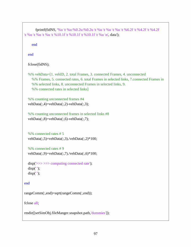
97

fprintf(fidNS, '%u \t %u:%0.2u:%0.2u \t %u \t %u \t %u \t %6.2f \t %4.2f \t %4.2f

\t %u \t %u \t %u \t %10.1f \t %10.1f \t %10.1f \t %u \n', data');

end

end

fclose(fidNS);

%% vehData=[1. vehID, 2. total Frames, 3. connected Frames, 4. unconnected

%% Frames, 5. connected rates, 6. total Frames in selected links, 7.connected Frames in

%% selected links, 8. unconnected Frames in selected links, 9.

%% connected rates in selected links]

%% counting unconnected frames #4

vehData(:,4)=vehData(:,2)-vehData(:,3);

%% counting unconnected frames in selected links #8

vehData(:,8)=vehData(:,6)-vehData(:,7);

%% connected rates # 5

vehData(:,5)=vehData(:,3)./vehData(:,2)*100;

%% connected rates # 9

vehData(:,9)=vehData(:,7)./vehData(:,6)*100;

disp('>>> >>> computing connected rate');

disp(' ');

disp(' ');

end

rangeComm(:,end)=sqrt(rangeComm(:,end));

fclose all;

rmdir([setSimObj.fileManger.snapshot.path,'dummies']);

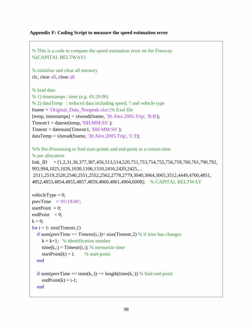
98

Appendix F: Coding Script to measure the speed estimation error

% This is a code to compute the speed estimation error on the Freeway

%(CAPITAL BELTWAY)

% initialize and clear all memory

clc, clear all, close all

% load data

% 1) timestamps : time (e.g. 05:20:00)

% 2) dataTemp : reduced data including speed, ? and vehicle type

fname = 'Original_Data_Nonpeak.xlsx';% Exel file

[temp, timestamps] = xlsread(fname, '30.Alex.2005.Trip', 'B:B');

Timestr1 = datestr(temp, 'HH:MM:SS' );

Timestr = datenum(Timestr1, 'HH:MM:SS' );

dataTemp = xlsread(fname, '30.Alex.2005.Trip', 'C:I');

%% Pre-Processing to find start-points and end-point in a certain time

% pre allocation

link_ID = [1,2,31,36,377,387,456,513,514,520,751,753,754,755,756,759,760,761,790,792,

993,994,1025,1026,1030,1106,1310,2416,2420,2425,...

2511,2519,2520,2540,2551,2552,2562,2778,2779,3040,3064,3065,3512,4449,4760,4851,

4852,4853,4854,4855,4857,4859,4860,4861,4904,6008]; % CAPITAL BELTWAY

vehicleType = 0;

prevTime = '05:19:00';

startPoint = 0;

endPoint = 0;

k = 0;

for i = 1: size(Timestr,1)

if sum(prevTime == Timestr(i,:))< size(Timestr,2) % if time has changes

k = k+1; % identification number

time(k,:) = Timestr(i,:); % memorize time

startPoint(k) = i; % start-point

end

if sum(prevTime == time(k,:)) ~= length(time(k,:)) % find end-point

endPoint(k) = i-1;

end

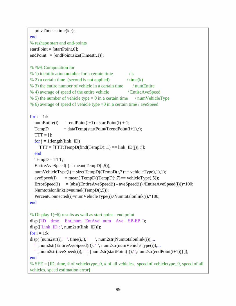
99

prevTime = time(k,:);

end

% reshape start and end-points

startPoint = [startPoint,0];

endPoint = [endPoint,size(Timestr,1)];

% %% Computation for

% 1) identification number for a certain time / k

% 2) a certain time (second is not applied) / time(k)

% 3) the entire number of vehicle in a certain time / numEntire

% 4) average of speed of the entire vehicle / EntireAveSpeed

% 5) the number of vehicle type = 0 in a certain time / numVehicleType

% 6) average of speed of vehicle type =0 in a certain time / aveSpeed

for i = 1:k

numEntire(i) = endPoint(i+1) - startPoint(i) + 1;

TempD = dataTemp(startPoint(i):endPoint(i+1),:);

TTT = [];

for j = 1:length(link_ID)

TTT = [TTT;TempD(find(TempD(:,1) == link_ID(j)),:)];

end

TempD = TTT;

EntireAveSpeed(i) = mean(TempD(:,5));

numVehicleType(i) = size(TempD((TempD(:,7)== vehicleType),1),1);

aveSpeed(i) = mean( TempD((TempD(:,7)== vehicleType),5));

ErrorSpeed(i) = (abs((EntireAveSpeed(i) - aveSpeed(i))./EntireAveSpeed(i)))*100;

Numtotalonlink(i)=numel(TempD(:,5));

PercentConnected(i)=numVehicleType(i)./Numtotalonlink(i).*100;

end

% Display 1)~6) results as well as start point - end point

disp ('ID time Ent_num EntAve num Ave SP-EP ');

disp(['Link_ID : ', num2str(link_ID)]);

for i = 1:k

disp( [num2str(i),' ', time(i,:), ' ', num2str(Numtotalonlink(i)),...

' ',num2str(EntireAveSpeed(i)), ' ', num2str(numVehicleType(i)),...

' ', num2str(aveSpeed(i)), ' ', [num2str(startPoint(i)),'-',num2str(endPoint(i+1))] ]);

end

% SEE = [ID, time, # of vehicletype_0, # of all vehicles, speed of vehicletype_0, speed of all

vehicles, speed estimation error]

100

SEE = [[1:k]',numVehicleType', Numtotalonlink', PercentConnected', aveSpeed',

EntireAveSpeed', ErrorSpeed'];

SEE_time = time;

Assessment of Vehicle-to-Vehicle Communication based ... · vehicles equipped with V2V...

Documents

Transcript of Assessment of Vehicle-to-Vehicle Communication based ... · vehicles equipped with V2V...