Assessment of turbulence effects on effective solute ...

ORIGINAL PAPER

Assessment of turbulence effects on effective solute diffusivity closeto a sediment-free fluid interface

E. Baioni1,2 • G. M. Porta2 • M. Mousavi Nezhad1 • A. Guadagnini2

Accepted: 5 September 2020 / Published online: 26 September 2020� The Author(s) 2020

AbstractOur work is focused on the analysis of solute mixing under the influence of turbulent flow propagating in a porous system

across the interface with a free fluid. Such a scenario is representative of solute transport and chemical mixing in the

hyporheic zone. The study is motivated by recent experimental results (Chandler et al. Water Res Res 52(5):3493–3509,

2016) which suggested that the effective diffusion parameter is characterized by an exponentially decreasing trend with

depth below the sediment-water interface. This result has been recently employed to model numerically downstream solute

transport and mixing in streams. Our study provides a quantification of the uncertainty associated with the interpretation of

the available experimental data. Our probabilistic analysis relies on a Bayesian inverse modeling approach implemented

through an acceptance/rejection algorithm. The stochastic inversion workflow yields depth-resolved posterior (i.e., con-

ditional on solute breakthrough data) probability distributions of the effective diffusion coefficient and enables one to

assess the impact on these of (a) the characteristic grain size of the solid matrix associated with the porous medium and

(b) the turbulence level at the water-sediment interface. Our results provide quantitative estimates of the uncertainty

associated with spatially variable diffusion coefficients. Finally, we discuss possible limitations about the generality of the

conclusions one can draw from the considered dataset.

Keywords Effective diffusion � Sediment-water interface � Stochastic model calibration � hyporheic region �Uncertainty quantification

1 Introduction

The hyporheic region is a major component driving func-

tioning of river ecosystems through regulation of processes

associated with, e.g., attenuation of pollutants by bio-

degradation or adsorption and mixing. All of these

processes are critically affected by chemical residence time

and mixing rate within the hyporheic zone, these being in

turn controlled by turbulent flow patterns which are doc-

umented to propagate across the interface between river

flow and the hyporheic region (Buss et al. 2009).

Major research findings on stream-subsurface solute

exchanges and feedbacks are summarized in Boano et al.

(2014) and Rode et al. (2015). Dissolved chemicals trans-

ported through stream flow are typically subject to a tem-

porary storage within the hyporheic zone beneath and/or

alongside the stream bed followed by subsequent release

into the water column. Our current framework of concep-

tual understanding and depiction of hyporheic exchange

processes is grounded on a set of empirical observations

and suggests that the characteristics of the stream flow and

sediments, along with the stream bottom topography (El-

liott and Brooks 1997), are the main drivers to flow and

mass exchange across the hyporheic zone (Lautz and Sie-

gel 2006). The hyporheic residence time, i.e., the time of

& M. Mousavi Nezhad

[email protected]

E. Baioni

[email protected]

G. M. Porta

[email protected]

A. Guadagnini

[email protected]

1 School of Engineering, University of Warwick,

Warwick CV47AL, UK

2 Dipartimento di Ingegneria Civile e Ambientale, Politecnico

di Milano, Milano, Italy

123

Stochastic Environmental Research and Risk Assessment (2020) 34:2211–2228https://doi.org/10.1007/s00477-020-01877-y(0123456789().,-volV)(0123456789().,-volV)

http://orcid.org/0000-0002-0625-439X

http://crossmark.crossref.org/dialog/?doi=10.1007/s00477-020-01877-y&domain=pdf

https://doi.org/10.1007/s00477-020-01877-y

retention of the solutes in the hyporheic zone, is then

chiefly controlled by transport characteristics such as pore

water velocity and dispersion as well as by the chemical

reactivity of the investigated compounds (Schaper et al.

2019). In this context, our study targets the characterization

of the uncertainty affecting the parameters describing

solute transport, in the hyporheic zone, in the absence of

chemical and biological reactive processes. Under these

conditions, solute spreading and mixing is driven by

molecular diffusion and by the local spatial and temporal

fluctuations of the fluid velocity. A description of

groundwater flow based on a classical continuum-scale

approach (often relying, e.g., on the Darcy equation) is

typically employed to study field-scale surface-groundwa-

ter interactions. While such an approach allows quantifying

water fluxes between subsurface and surface water bodies,

it neglects the effects of several physical processes that are

known to influence solute residence time and mixing in the

hyporheic zone (Woessner 2000). In particular, complexi-

ties of hyporheic exchanges are mainly tied to molecular

diffusion, shear-driven flow, advective phenomena arising

in the presence of river bed forms (also termed as advective

pumping) and propagation of turbulence from the river

stream into the hyporheic region (O’Connor and Harvey

2008; Chandesris et al. 2013). In practice, approaches

employed to estimate hyporheic solute exchanges rely on

effective models, somehow embedding the effects of all

these processes (Lautz and Siegel 2006). Widely known

examples of these effective approaches are the transient

storage model (TSM) (Bencala 1983; Hart 1995; Triska

et al. 1989; Worman 2000) the pumping model (PM) (El-

liott and Brooks 1997; Packman and Brooks 2001; Pack-

man et al. 2000), and the slip flow model (SFM) (Fries

2007). Ultimately, the aim of all these models is to provide

predictions of downstream solute transport, this objective

being achieved by embedding specific parameters repre-

senting hyporheic solute exchange. In TSM the stream-bed

exchange is evaluated considering (a) a storage zone, i.e.,

the upper region of the bed sediments, which is typically

assumed to be characterized by a constant depth, and (b) a

mass transfer process, which is formulated through an

effective parameter. The exchange is assumed to be pro-

portional to the difference of solute concentrations in the

main channel and the storage zone (Bencala 1983).

Experimental data such as those reported in Chandler et al.

(2016) can be employed to constrain the parameters of

TSM, as the latter approach relies on a conceptualization of

hyporheic exchange in terms of solute transfer between two

physical domains, i.e. main stream and bed sediments.

Several mathematical formulations of such a conceptual

model have been proposed in Rutherford et al. (1995),

Tonina and Buffington (2007), Worman (1998). In PM and

SFM solute transport is assumed to be advection-

dominated, flow across the sediment bed being governed

by Darcy’s Law. The exchange at the sediment-water

interface is driven by pressure (i.e., head distribution) or

shear velocity (velocity distribution) in PM or SFM,

respectively. Molecular diffusion and turbulence effects are

neglected in both models. The investigation of the influ-

ence of physical quantities such as grain size and bed shear

velocity on the diffusive transport across the sediment-

water interface is a significant part of our study. PM

describes the solute exchange process as a function of

quantities characterizing the stream and sediment attri-

butes, such as sediment permeability, channel geometry

and stream velocity (Elliott and Brooks 1997; Marion et al.

2003). Particle-based continuous time random walk

(CTRW) approaches have also emerged in the past decade

as alternatives to the above-mentioned continuum-based

effective approaches (Boano et al. 2007; Sherman et al.

2019).

Our work tackles the characterization of the spatial

distribution of mixing and diffusion parameters in the

hyporheic zone which is a key element for all of the above

mentioned methodologies. To improve the quality of this

characterization, propagation of turbulence from the river

flow into the hyporheic region has been quantified through

experiments (Chandler et al. 2016; Higashino et al. 2009;

de Lemos 2005; Roche et al. 2019) and numerical simu-

lations (Bottacin-Busolin 2019; Breugem et al. 2006;

Sherman et al. 2019; Chandesris et al. 2013). Notably, in

this context we refer to the high resolution experimental

data collected by Chandler et al. (2016). Previous studies

show the possibility of describing vertical mixing through

an effective diffusion model. In these works, the authors

quantify the variation of the effective diffusion coefficient

with depth below the interface for various bed shear

velocity and grain size combinations in the presence of

turbulent flow conditions taking place above a flat sedi-

ment-water interface. The experimental evidences are

interpreted upon relying on the analytical solution pro-

posed by Nagaoka and Ohgaki (1990) and the authors

conclude that the diffusion coefficient can be described by

an exponential reduction with depth. In this framework, it

is noteworthy to observe that also the periodic advection of

turbulent eddies across the sediment-water interface exhi-

bits an exponential decrease with depth underneath the

stream bed (Bottacin-Busolin and Marion 2010). These

results are at the basis of current practices that rely on

embedding an exponential reduction (along the vertical) of

effective diffusion effects in modeling frameworks (Bot-

tacin-Busolin 2019; Roche et al. 2019). These studies have

shown that assuming an exponential reduction of the dif-

fusion coefficient (a) has relevant implications on the

modeling of solute mixing in streams, (b) is consistent with

model-based interpretations of observed reach-scale

2212 Stochastic Environmental Research and Risk Assessment (2020) 34:2211–2228

123

transport experiments. Assumptions on the spatial distri-

bution of the diffusion coefficient (e.g., either constant or

piece-wise uniform along the sediment bed) can markedly

impact the strength of solute exchange and mixing across

the surface water interface and thereby influence solute

breakthrough times at downstream locations. While the

experimental findings of Chandler et al. (2016) have been

extensively used within transport model formulations, the

uncertainty associated with the interpretation of the dataset

has not yet been addressed and quantified.

Our main objective is to analyze the variability of the

effective diffusion coefficient within a probabilistic per-

spective upon relying on a stochastic inverse modeling

approach. We recall that stochastic calibration enables one

to evaluate the probability density function (pdf) of each

(unknown) model parameter conditional to the available

dataset, i.e., the posterior parameter density. Otherwise, a

deterministic approach focuses on identifying a unique set

of model parameters that minimizes a target objective

function. Chandler et al. (2016) obtain estimates of the

diffusion coefficient below the sediment-water interface by

following the procedure outlined in Nagaoka and Ohgaki

(1990) and considering a simple mean square error as a

metric of model performance, following a typical deter-

ministic optimization procedure.

In our study we consider solute concentration data col-

lected during the experiments of Chandler (2012) (see Sect.

2.1) and ground our stochastic analysis on the acceptance/

rejection methodology (Gelman et al. 2013; Tarantola

2005) to estimate the posterior (i.e., conditional on avail-

able observations) probability distribution of the diffusion

coefficient which is then propagated to provide a proba-

bilistic depiction of the ensuing chemical concentrations at

diverse depths in the system. Our study considers various

combinations of bed shear velocity and grain size, as

embedded in the dataset analyzed. As such, the key

objective of our work is the assessment of the robustness of

the typically employed exponential decay relationship

between the diffusion coefficient and depth (Chandler

2012; Chandler et al. 2016) and the quantification of the

related uncertainty. While, as mentioned above, the

assumption of the exponential decrease of effective diffu-

sion (and ensuing mixing) below the stream bed is

increasingly adopted in modeling studies, to the best of our

knowledge the only experimental evidence directly sup-

porting such a behavior is the one reported in Chandler

et al. (2016). The results stemming from our contribution

may then be useful to propagate parametric uncertainty to

reach-scale models, as recently advocated in Tu et al.

(2019).

The structure of the work is described in the following.

Section 2 is devoted to the illustration of the methodology

employed for stochastic model calibration through the

acceptance/rejection method. The reference experimental

setup of Chandler et al. (2016) and the analytical solution

employed in the calibration workflow are presented in

Sect. 2.1. Sect. 3 exposes the key results of the study.

Finally, concluding remarks are provided in Sect. 4.

2 Methodology and problem setup

In the following we describe the setup and experimental

data we consider in this study as well as the stochastic

model calibration procedure we employ.

2.1 Reference experimental setup

We provide here a brief description of the reference

experimental tests performed by Chandler (2012) which

form the basis of the calibration dataset we consider. The

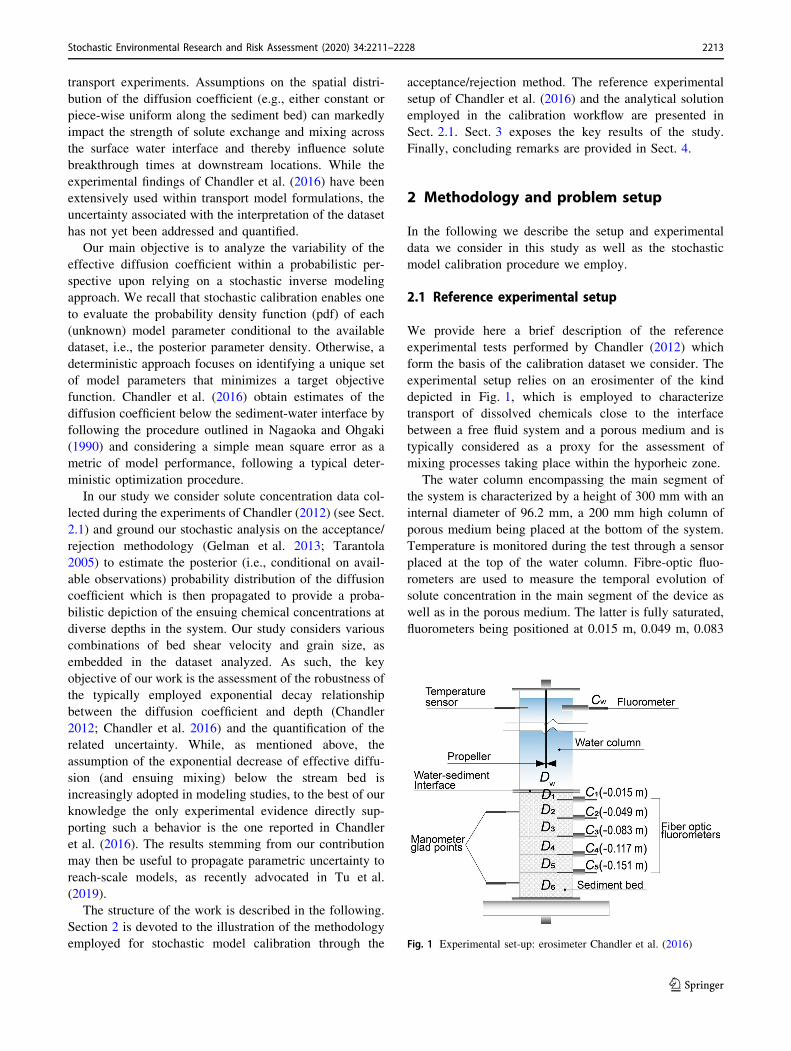
experimental setup relies on an erosimenter of the kind

depicted in Fig. 1, which is employed to characterize

transport of dissolved chemicals close to the interface

between a free fluid system and a porous medium and is

typically considered as a proxy for the assessment of

mixing processes taking place within the hyporheic zone.

The water column encompassing the main segment of

the system is characterized by a height of 300 mm with an

internal diameter of 96.2 mm, a 200 mm high column of

porous medium being placed at the bottom of the system.

Temperature is monitored during the test through a sensor

placed at the top of the water column. Fibre-optic fluo-

rometers are used to measure the temporal evolution of

solute concentration in the main segment of the device as

well as in the porous medium. The latter is fully saturated,

fluorometers being positioned at 0.015 m, 0.049 m, 0.083

Fig. 1 Experimental set-up: erosimeter Chandler et al. (2016)

Stochastic Environmental Research and Risk Assessment (2020) 34:2211–2228 2213

123

m, 0.117 m, and 0.151 m below the sediment-water

interface.

Turbulence is generated at the top of the base segment

through a tri-bladed propeller positioned at a distance of 40

mm from the water-soil interface. The propeller speed is

tuned to produce a bed shear velocity favoring a setting

corresponding to the onset of sediment motion Chandler

et al. (2016). The porous bed is initially saturated with a

tracer (fluorescein disodium salt), whose concentration in

the water column is null. Various combinations of bed

shear velocity (u) and characteristic grain size (dg) of the

porous medium are analyzed in the experiments. Values of

the experimental parameters and corresponding estimates

of diffusion coefficients are listed in Table 1.

2.2 Analytical solution

Assuming that mass transfer can be described as a one-

dimensional (along the vertical direction) process, solute

transport within the porous system is modeled through:

oCðt; yÞot

¼ o

oyDðyÞ oCðt; yÞ

oy

� �ð1Þ

Here, C(t, y) [ML�3] is solute mass concentration, y [L] is

the distance from the exchange interface, D [L2T�1] is an

effective diffusion coefficient, and t is time. We recall that

D is considered as an effective model parameter which

embeds a continuum-scale description of pore-scale pro-

cesses. We follow the methodology proposed in Chandler

et al. (2016) and employ the analytical solution for Eq. (1)

proposed by Nagaoka and Ohgaki (1990) to analyze the

depth-dependent variation of the diffusion coefficient.

These authors consider the domain to be composed by NL

layers. An analytical formulation is then derived for a basic

system comprising two layers separated by an interface at

y ¼ �L and characterized by effective diffusion coeffi-

cients D ¼ Di for 0\y\� L and D ¼ Diþ1 for

ð�L\y\�1Þ, respectively (see the sketch in Fig. 2).

Boundary and initial conditions for Eq. (1) are set as:

Cð0; yÞ ¼ 0 ð2Þ

Cðt; 0Þ ¼ f ðtÞ ð3Þ

Cðt;�L�Þ ¼ Cðt;�LþÞ ð4Þ

limy!�1

Cðt; yÞ ¼ 0 ð5Þ

DidCdy

jy¼�L� ¼ Diþ1

dCdz

jy¼�Lþ ð6Þ

Considering a system of NL layers, solute concentration

at the interface between two layers (corresponding, i.e., at

y ¼ �L in the setting of Fig. 2) can be evaluated analyti-

cally as Nagaoka and Ohgaki (1990):

Ci½f ðtÞ;Di;Diþ1; L� ¼L

ðbþ 1ÞffiffiffiffiffiffiffiffipDi

pZ t

0

f ð�Þðt � �Þ

32

X1k¼0

ckð2k þ 1Þe�ð2kþ1Þ2L24Diðt��Þ d�

ð7Þ

Here, index i ¼ 2; . . .;NL � 1 indicates the layer number,

b ¼ffiffiffiffiffiffiffiDiþ1

Di

q, c ¼ b�1

bþ1, L ¼ yi � yi�1 is the (vertical) distance

between two layers, f(t) corresponds to concentration

observed at yi�1 and t is total duration. Relying on Eq. (7)

enables one to estimate the diffusion coefficient of the

upper layer (Di) once the diffusion coefficient at the lower

layer (Diþ1) and the temporal dynamics of concentration at

the top of the upper layer (f(t)) are known. For the lowest

layer (i.e., i ¼ NL), we follow Nagaoka and Ohgaki (1990)

and assume that the corresponding diffusion coefficient

coincides within the one associated with the layer above it,

thus obtaining

Table 1 Values of the estimated

diffusion coefficients reported

in Chandler et al. (2016) for the

experimental conditions

examined

u [m/s]

0.015 0.01

Test1_1 Test1_2 Test2_1 Test2_2

dg [mm] 5 Layer 2 1.91E-06 2.79E-06 1.62E-06 1.28E-06

Layer 3 5.30E-07 4.85E-07 4.32E-07 3.26E-07

Layer 4 4.39E-08 6.98E-08 1.42E-08 3.61E-08

Layer 5 2.90E-09 6.70E-09 2.60E-09 2.70E-09

Test3_1 Test3_2 Test4_1 Test4_2

0.625 Layer 2 2.10E-08 1.87E-08 9.60E-09 1.27E-08

Layer 3 5.70E-09 5.20E-09 2.80E-09 2.80E-09

Layer 4 8.00E-10 1.00E-09 / /

Layer 5 / / / /


123

CNL½f ðtÞ;Di� ¼

L

2ffiffiffiffiffiffiffiffipDi

pZ t

0

f ð�Þðt � �Þ

32

e� L2

4Diðt��Þd� ð8Þ

Eqs. (7), (8) have been employed by Chandler et al. (2016)

to estimate values of effective diffusion coefficients Di in

the experimental column by replacing f(t) with observa-

tions. In Nagaoka and Ohgaki (1990) model calibration is

structured according to the following steps: (a) estimation

of the value of the diffusion coefficient in the lowest layer

upon constraining Eq. (8) through concentration values

sampled at the lowest available measurement location and

(b) estimation of coefficients Di (once Diþ1 is estimated)

through Eq. (7). A schematic depiction of the procedure is

offered in Fig. 3. Hereafter we denote the coefficients

estimated according to this procedure as ~Di, to distinguish

them from the result of our stochastic model calibration

approach.

2.3 Acceptance/rejection method

We ground our stochastic model calibration analyses on the

acceptance/rejection sampling (ARS) approach (see, e.g.,

Gelman et al. (2013), Tarantola (2005)). In this framework,

our objective is to assess the posterior pdf of the effective

diffusion parameter at a given depth yi (See Sect. 2.1), i.e

the location of each interface, starting from an assumed

prior distribution. In the context of ARS, one aims at

obtaining multiple independent Monte Carlo realizations of

the model output (in our case, solute concentrations at

locations corresponding to monitoring ports) by sampling

from the parameter distribution conditional to observations.

At each iteration j model parameter values are indepen-

dently sampled across the support within which the cor-

responding prior distribution is defined, the analytical

solution (Eqs. (7), (8)) is evaluated, and the candidate

parameter set is accepted or rejected upon relying on

threshold criteria based on the likelihood function. Key

details of the ARS are provided in the following.

Let C�i be a vector whose entries correspond to observed

values of concentrations at depth yi for a collection of N�

discrete time levels and Ci;j the corresponding values of

concentration obtained by applying Eq. (7) or (8) at depth

y ¼ yi and iteration j for the same time levels at which data

are available. We randomly sample the assumed prior

distribution of diffusion coefficients. The likelihood aj isdefined as:

aj ¼ e

�1

2r2Cy

ðC�i �Ci;jÞT ðC�

i �Ci;jÞ ð9Þ

where r2Cyis the variance associated with observation

errors (which are assumed to be zero-mean Gaussian).

The workflow depicted in Fig. 4 is employed for the

implementation of ARS to all layers except for Layer 1,

because no concentration data are available at the interface

between the water column and the porous medium.

The procedure is repeated until a collection of NR

accepted realizations is obtained or a maximum number of

iterations is reached. Accepted values are used to assess the

posterior probability distributions of the diffusion coeffi-

cients. Hence, as a result of the workflow we obtain a

bivariate sample of accepted parameters values, i.e., Si ¼½Di;Diþ1� for each pair of layers (with the exception of the

univariate sample Di for i ¼ NL), from which a sample/

empirical posterior probability distribution can be evalu-

ated. The value of the maximum a posteriori (MAP) can

then be approximated on the basis of the mode (i.e., the

maximum value) of the posterior. Relying on the MAP is

tantamount to considering the most likely value of the

investigated parameter within each layer (Murphy 2012).

We point out that reliance on the analytical Eqs. (7), (8)

implies that ARS is applied to two adjacent layers, the

Fig. 2 Graphical depiction of the boundary and initial conditions

corresponding to Eq. (2) and employed for the analytical solution of

Eq. (1)

Fig. 3 Schematic representation of the procedure employed to

estimate the effective diffusion coefficient of each layer in the

considered experimental setup (see also Nagaoka and Ohgaki (1990))


123

Fig. 4 Workflow of the

acceptance/rejection method

Tarantola (2005)


123

complete set of results being obtained through application

of ARS to all pairs of adjacent layers in the system. It

should be noted that we obtain two diverse posterior dis-

tributions for parameter Di associated with locations yi(with i[ 2 and i\NL) because the effective diffusion

coefficients are assessed in pairs in the workflow described

above. This is consistent with analytical Eqs. (7), (8) so

that each iteration of the ARS associates two values for the

diffusion coefficients Di with a given layer. These corre-

spond to (a) the one obtained from considering Layers i

and iþ 1 and (b) the one stemming from the analysis of

Layer i� 1 and Layer i, respectively.

To exemplify and clarify this point, we focus here on

three consecutive layers (Layer 3, 4, and 5). Once the

model has been calibrated for each pair of layers sepa-

rately, we obtain D4 1 and D5 from model calibration on

the solute breakthrough curve at the interface between

Layer 4 and 5 (i.e., considering C4�ðtÞ), D3 and D4 2 being

assessed in a corresponding way upon considering C3�ðtÞ.

We present our results in terms of both MAP values of the

diffusion coefficient within each layer. This information

can be useful to appraise conditions under which the

thickness of a given layer can be considered as large

enough to (a) allow process interpretations relying on

solutions for unbounded domains or (b) assess the influence

of boundary conditions on the system behavior. Criteria for

the selection of the representative diffusion coefficient at

each layer are clarified in Sect. 3.

The support of the prior distribution of the diffusion

coefficients is here centered around the estimated values

provided in Chandler et al. (2016) and is taken to span two

orders of magnitude. For example, if ~Di is of the order 10�9

m2=s, the maximum and minimum value of the support of

the prior pdf are taken as 10�8 m2=s and 10�10 m2=s,

respectively. Whenever the resulting value DiðMAPÞ is tooclose to (or coincides with) either of its limits the support

of the prior distribution is widened and the ARS algorithm

is restarted. We note that some values of the effective

diffusion coefficient are not listed in Chandler et al. (2016),

possibly due to some difficulties encountered during model

calibration. For those cases we set the width of the support

of the prior around the value corresponding to a best fit (as

evaluated according to a standard least-square regression)

between the analytical solution and the experimental data.

Here, we rely on stochastic procedure to obtain posterior

distributions of diffusion coefficients also for such layers.

The available experimental data (Chandler et al. 2016)

correspond to measurements of the solute concentration at

various depths under the sediment-water interface for

various combination of grain size and bed shear velocity.

For each scenario (sediment diameter/bed shear velocity),

the test is repeated twice and the average of the two series

of laboratory data is used as input in the acceptance/re-

jection procedure. Our analysis encompasses the conditions

corresponding to the various experimental settings listed in

Table 1, as expressed in terms of combinations of grain

size (dg) and bed shear velocity (u).

The experimental data are selected to ensure an accurate

representation of the experimental trend. Experimental data

show that equilibrium of solute concentrations at locations

close to the sediment-water interface is attained at early

stage (i.e., t� 5000s for Test 1 and 2 and t� 200000s for

Test 3 and 4). Hence, model calibration at the interface

Layer 2-Layer 3 is performed considering the experimental

solute breakthrough curves prior to steady-state to allow

for a reduced computational time. Otherwise, solute con-

centrations at deeper layers exhibit a slow reduction across

time, a feature which is mainly seen in the scenario char-

acterized by small sediment size. In order to reduce the

computational load without losing accuracy, the experi-

mental data at these locations are selected using a time

resolution coarser than the one employed for the collection

of the laboratory measurements. No smoothing filters are

applied on the experimental data.

3 Results

We start the illustration of our results by noting that all

concentration data are reported in [%], a value of 100

corresponding to the initial concentration in the porous

medium. Since no details on measurement uncertainty is

reported by Chandler et al. (2016), the measurement error,

rCy, is here fixed to 25% with the exception of the cali-

bration scenario associated with the pair Layer 2- Layer 3

for which we consider rCy= 45%. These values have been

selected after a series of preliminary analyses to ensure an

acceptance rate at least equal to 0.1%.

Figures 5 and 6 document the results obtained in terms of

the probability distributions for the effective diffusion

coefficients. Figure 5 depicts empirical bivariate distribu-

tions for the diffusion coefficients associated with the

observations pertaining to Test 1 (including the sample

posterior distribution for D5 obtained when considering

Eq. (8) to interpret only data from Layer 5), Fig. 6 depicting

the resulting concentration histories at various depths. Cor-

responding results obtained for Tests 2-4 are included in

Appendix A. The solute breakthrough curves in Fig. 6 are

evaluated from Eqs. (7), (8) where values of diffusion

coefficients estimated for each pair of layers are employed.

For example, the concentration C4 at the interface between

Layer 4 and Layer 5 is evaluated using the MAP value of the

diffusion coefficients D4 and D5 resulting from model cali-

bration for the pair Layer 4-Layer 5.


123

Figure 5 and the results included in Appendix A

(Fig. 10) clearly show that the values of the diffusion

coefficients estimated by Chandler et al. (2016), i.e., ~Di,

reside within the range of the values identified through

ARS. An analogous behavior is documented for the

remaining experimental tests for which estimates ~Di are

available (Fig. 10 in Appendix A). We note that the results

depicted in Fig. 5 are obtained upon considering rCy¼

45% for the pair Layer 2-Layer 3, as opposed to the value

of 25% employed for all of the remaining layers. We note

that as a first attempt we set rCy¼ 25% for all layers.

Although this choice resulted in a generally reasonable

compromise between a good acceptance rate and the loss of

the quality of the data, a negligible acceptance rate was still

noted when considering the shallowest layer (see Fig. 7).

While we recognize that the magnitude of measurement

errors is only assumed in our study, as no precise infor-

mation on this aspect is available, we also note that such

low acceptance rate is consistent with the observations that

(i) one can argue that the turbulent behavior of flow at

locations close to the sediment-water interface may influ-

ence the accuracy of the data at shallow depths more

markedly than at larger depths, and (ii) data interpretation

rests on a simplified diffusive model whose skill to repre-

sent the process may decrease close to the sediment-water

interface. As an additional element, which might suggest

that turbulence is related to highest measurement uncer-

tainties at the shallowest layer, we observe that the need to

assume the largest measurement errors at the shallowest

layer was linked to all tests, independent from the sediment

size. Therefore, the value of rCywas progressively

increased until a reasonable acceptance rate was attained.

A value rCy¼ 45% is employed for the shallowest layers.

While considering rCy\45% would provide a sufficient

number of accepted diffusion coefficient values in Test 1

(see Fig. 7), for the sake of uniformity we decided to

employ the same values of measurement error in all tests.

Non-zero values of posterior distributions associated

with the deepest layers (Layers 4 and 5) and the smallest

grain diameters tested (Tests 3 and 4) are found across a

Fig. 5 Sample probability

density and joint-relative

frequency resulting from the

stochastic inverse modeling

approach for Test 1: a D3-D2,

b D4-D3, c D5-D4 d pdf D5. The

red and magenta dots represent

the values reported by Chandler

et al. (2016) for the two

replicates of this Test. We

consider rCy¼ 25% for the

calibration of D5, D5 � D4,

D4 � D3, while rCy¼ 45% for

the pair D3 � D2


123

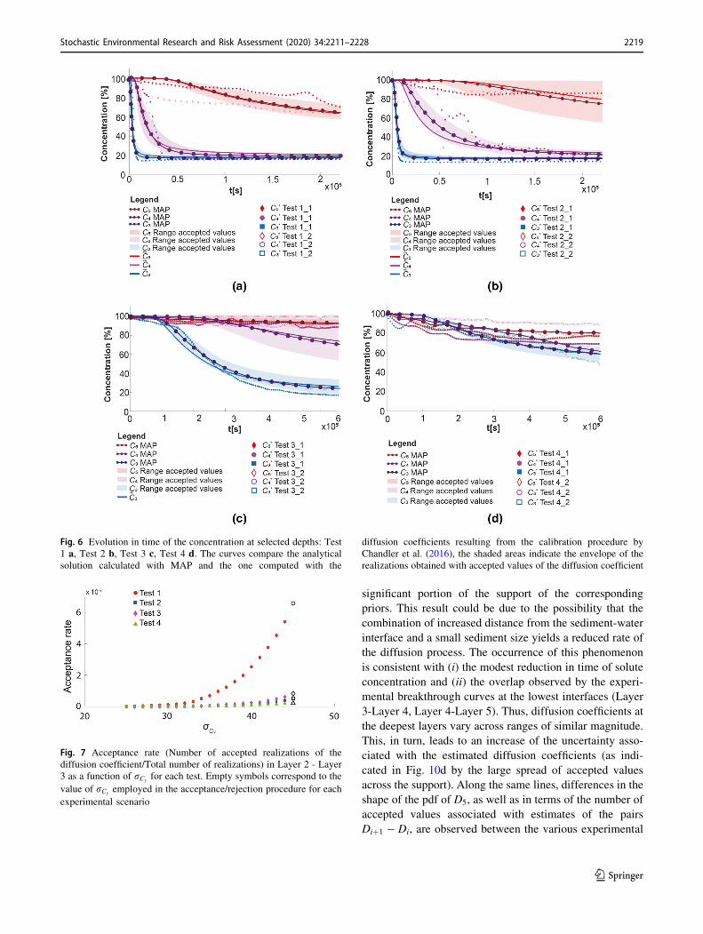
significant portion of the support of the corresponding

priors. This result could be due to the possibility that the

combination of increased distance from the sediment-water

interface and a small sediment size yields a reduced rate of

the diffusion process. The occurrence of this phenomenon

is consistent with (i) the modest reduction in time of solute

concentration and (ii) the overlap observed by the experi-

mental breakthrough curves at the lowest interfaces (Layer

3-Layer 4, Layer 4-Layer 5). Thus, diffusion coefficients at

the deepest layers vary across ranges of similar magnitude.

This, in turn, leads to an increase of the uncertainty asso-

ciated with the estimated diffusion coefficients (as indi-

cated in Fig. 10d by the large spread of accepted values

across the support). Along the same lines, differences in the

shape of the pdf of D5, as well as in terms of the number of

accepted values associated with estimates of the pairs

Diþ1 � Di, are observed between the various experimental

Fig. 6 Evolution in time of the concentration at selected depths: Test

1 a, Test 2 b, Test 3 c, Test 4 d. The curves compare the analytical

solution calculated with MAP and the one computed with the

diffusion coefficients resulting from the calibration procedure by

Chandler et al. (2016), the shaded areas indicate the envelope of the

realizations obtained with accepted values of the diffusion coefficient

Fig. 7 Acceptance rate (Number of accepted realizations of the

diffusion coefficient/Total number of realizations) in Layer 2 - Layer

3 as a function of rCyfor each test. Empty symbols correspond to the

value of rCyemployed in the acceptance/rejection procedure for each

experimental scenario


123

tests (see Figs. 5 and 10). For example, in Test 4, where

the experimental breakthrough curves C5�,C4

� are essen-

tially overlapped, the presence of multiple peaks in the pfd

of D5 (see Fig. 10 ((iii)-d)) can introduce elements of

ambiguity in the interpretation, as opposed to the remain-

ing. We further note that decreased concentration values

are observed at shallow locations at early times, where the

diffusion model employed may be inaccurate due to effects

of marked spatial concentration gradients. Additionally as

these points are located close to the sediment-water inter-

face, transport involves small space-time scales, and may

exhibit a non-Fickian pre-asymptotic behaviour. We

observe a good agreement between the CiðMAPÞ and ~Ci in

Test 1, the ensuing results being virtually indistinguishable

for Layer 5 and displaying only minor differences for

Layers 3 and 4. The trends displayed by the experimental

observations are reasonably well reproduced by the mod-

eling results, even as local oscillations in the concentration

temporal gradients are not represented through the diffu-

sive model. With reference to the latter point, the observed

concentration C�4 appears to display a steeper decrease than

the corresponding model results, which display a reduced

rate of convergence to the final (equilibrium) concentration

(that is approximately equal to 20%). Experimentally

observed concentrations within Layer 5 (i.e., C�5) initially

decrease faster than their model-based counterparts.

Otherwise, we observe that the values C5ðMAPÞ are close

to the experimental observations for long times

(t[ 0:75� 105 s).

We recall that, considering a given pair of layers in the

model calibration procedure of Nagaoka and Ohgaki

(1990), the pattern of solute concentration at the top of the

upper layer plays a significant role on the determination of

the breakthrough curve at the interface between the layers.

In other words, and referring to the bottom layer, the

behavior displayed by C5ðMAPÞ calculated from Eq. (8)

using as input values the diffusion coefficient D4ðMAPÞ,D5ðMAPÞ, and the experimental concentration C4

�, is

considerably affected by the temporal variation of the lat-

ter. The strong dependence between C5ðMAPÞ and C4�

may contribute to the discrepancy observed between C5�

and C5ðMAPÞ.Results of corresponding quality are obtained for Test 2

and Test 3 (Fig. 6b,c). Estimated C5ðMAPÞ and C3ðMAPÞvalues in Test 3 (Fig. 6c) display a temporal pattern which

is in close agreement with their experimental counterpart

(see in C�5 Test 3 1 and in C�

3 Test 3 2, respectively).

Otherwise, an increased discrepancy can be observed

between the experimental data and their model-based

counterparts for C4, the latter (i.e., C4ðMAPÞ and ~C4)

decreasing faster than the experimentally-based results and

attaining a final concentration which is 20% lower than the

experimental one.

With reference to Test 4 (Fig. 6d), we note that only

CiðMAPÞ values can be compared against the experimental

data set, as estimated values for the effective diffusion

coefficient are not documented by Chandler (2012),

Chandler et al. (2016). The analytical curve C5ðMAPÞexhibits a behavior which is similar to the experimental

one, i.e., C�5 Test4 2. A similar result is observed for the

curve C3ðMAPÞ for t[ 105 s. On the other hand, model

results corresponding to C4ðMAPÞ decrease following a

trend significantly different from the one displayed by the

experimental data. We observe that Test 4 displays similar

late-time slopes for the experimental curves associated

with C3�, C4

�,C5�, differing slopes being observed in the

remaining tests. As mentioned above, estimation of the pair

of coefficients D2 � D3 using concentration data C�2 is

characterized by a significantly reduced acceptance rate as

compared to the remaining layers. As such, it has been

subject to a specific analysis.

Figure 7 depicts the results of the investigations corre-

sponding to increasing values of rCy, to investigate the

impact of measurement errors on the acceptance rate, the

latter being quantified as the ratio between the number of

accepted pairs D2 � D3 and the total number of realizations

tested. As stated earlier, the rationale underlying this

analysis corresponds to the observation that measurement

(and model) error may increase as sampling locations are

closer to the interface between the porous medium and the

water. As shown in Fig. 7, the highest acceptance rate is

associated with the experiments characterized by the lar-

gest grain size and bed shear velocity (i.e., Test 1), while

the lowest acceptance rate corresponds to the scenario with

the smallest grain size and lowest velocity (i.e., Test 4), the

remaining two tests being positioned between these two

extremes. This analysis suggests that the data quality is not

uniform across the tests: parameter estimation in Test 1

appears to be associated with lower measurement errors

than in the remaining settings, while data of Test 4 tend to

be characterized by the lowest reliability (i.e., the largest

estimated measurement error). This result is consistent with

the observation that Chandler (2012), Chandler et al.

(2016) did not report results associated with effective dif-

fusion estimates in Test 4.


123

Our results indicate that acceptance rates increase with

the grain diameter and with bed shear velocity, thus sug-

gesting that the quality of the data and the ability of the

considered diffusion model to interpret these are directly

influenced by these two physical parameters. This result

may also be related to the specific equipment employed

during the tests. For example, the sensors used to measure

concentrations are sensitive to temperature variations. As

experiments characterized by small grain diameters are

associated with a longer duration, the related measurements

may display a time dependent error which is hard to model

explicitly in the absence of further information. We

observe that the overall performance of the model con-

sidered (i.e., Eqs. (7), (8)) is less satisfactory for the shal-

lowest layers, a significant discrepancy between the

temporal pattern of C2ðMAPÞ and its experimental coun-

terpart (C�2) being observed at Layer 2 (see Fig. 11 in

Appendix B) in all tests.

We then investigate the influence of the grain size and

the bed shear velocity on the diffusion process and assess if

the signature of the exponential reduction of the diffusion

coefficient with depth reported in the literature Chandler

et al. (2016) is observed also through our results. We do so

by normalizing the vertical coordinate below the water-

sediment interface through the characteristic sediment size

(dg), the diffusion coefficient being normalized by ðudgÞ.The results of the stochastic calibration process are then

summarized in Fig. 8, where one can also compare the

MAP parameter values resulting from the acceptance/re-

jection procedure against the corresponding estimates

obtained by Chandler et al. (2016). We recall that exam-

ining two consecutive pairs of layers yields two distinct

values for the diffusion coefficient of a given layer. As

such, two values of the MAP (red squares) are displayed at

each layer in Fig. 8.

Fig. 8 Summary of the acceptance/rejection stochastic calibration results for all experimental tests: a Test 1, b Test 2, c Test 3, d Test 4, and the

corresponding regression fits


123

A graphical depiction of the acceptance range corre-

sponding to the 25th and 75th percentile is included in

Fig. 8 for each MAP value, thus providing quantitative

information on the uncertainty about the estimated diffu-

sion coefficient at each layer. Furthermore, our results

allow quantifying the range of variability of accepted

values for a given layer which stems from analyzing the

results of two consecutive pairs of layers, i.e., an estimate

of Di is obtained through the concentration histories C�i and

C�i�1. These two estimates are here obtained independently

and results in Fig. 8 show that they identify distinct ranges

for each Di. This result is possibly related to the different

role played by the same coefficients in the two consecutive

steps and suggests that the workflow proposed in Nagaoka

and Ohgaki (1990) and depicted in Fig. 3 may not lead to

optimal estimation results. In the following we consider for

each coefficient Di only the probability distribution

obtained using the data C�i , consistent with the interpreta-

tion given in Nagaoka and Ohgaki (1990).

We consider next the following relationship suggested

by Chandler (2012) to characterize the dependence

between (dimensionless) effective diffusion and depth

y

dg¼ A � log D

dg � u

� �þ B ð10Þ

Here, A and B are model parameters which we estimate by

linear regression, upon substituting the values of ~Di or

DiðMAPÞ in (10). The results of such an analysis are listed

in Table 2.

As shown in Fig. 8, our result display an exponential

reduction of the diffusion coefficient with depth for Tests 1

and 2, i.e., for a grain size of dg ¼ 5 mm. Otherwise, the

occurrence of a decreasing pattern is not consistent with the

results obtained for Tests 3 and 4, i.e., for dg ¼ 0:625 mm.

In Test 3, we observe a decay of the diffusion coefficient

up to Layer 4, results obtained for Layer 5 being incon-

sistent with the trend found by Chandler et al. (2016). We

observe that the effective diffusion coefficient displays an

increasing trend with depth for y=dg\� 100 in Test 4.

This behavior is not supported by a well-defined physical

interpretation. Note that, as mentioned above, concentra-

tion values observed at different depths for Test 4 display

minimal differences (see Fig. 6). Similarly, concentrations

observed in layers 4 and 5 in Test 3 display no appreciable

decreasing trend (see Fig. 6d). These observations suggest

that the available time series are too limited to enable a

detailed assessment and quantification of the transport

process taking place under these conditions and for

y=dg\� 100.

Figure 9 juxtaposes the collection of values DiðMAPÞobtained for each experimental test analysed. We observe

that the results obtained for Test 1 are similar to those of

Tests 2. Otherwise, results obtained for Tests 3 and 4 fol-

low a different trend. The results depicted in Fig. 9 suggest

that recasting the problem in terms of dimensionless

parameters of the kind included in Eq. (10) does not pro-

vide a unique interpretation to the available data and that

the exponential trend may be representative solely of the

grain diameters analyzed. While a physical explanation of

the observed behavior is not clear at the current stage, the

analysis of additional experimental data would be required

to shed more light on this element.

4 Discussion and conclusions

Our study is aimed at the quantification of the uncertainty

associated with effective diffusion coefficients employed to

describe solute transport and mixing in the hyporheic

region. We do so upon relying on a set of experiments

performed at the laboratory scale considering solute

transport close to a sediment-water interface (Chandler

2012; Chandler et al. 2016). These are associated with

various combinations of (a) bed shear velocity, governing

the intensity of turbulent fluxes propagating from the water

body to the underlying porous bed, and (b) characteristic

size of the grains forming the solid matrix of the porous

medium. Similar to the analysis of Chandler (2012) and

Chandler et al. (2016), we rely on the analytical formula-

tion of Nagaoka and Ohgaki (1990) as our process model.

Our analysis then rests on a stochastic inverse modeling

approach based on the acceptance/rejection algorithm. Our

findings contribute to enhance the information content

associated with the results in Chandler et al. (2016), as we

provide a quantification of the uncertainty associated with

estimated diffusion coefficients. Our study explicitly yields

the posterior (i.e., conditional to observations) distribution

Table 2 Values of coefficients A and B in Eq. (10) and corresponding

R2 resulting from linear regression

A B R2

Test 1 D(MAP)_Test 1 2.4726 0.1281 0.9142

D_Test 1_1 3.0258 3.2895 0.9772

D_Test 1_2 3.3792 4.2913 0.9955

Test 2 D(MAP)_Test 2 2.7644 3.5088 0.9042

D_Test 2_1 2.9063 2.4712 0.9713

D_Test 2_2 3.2293 4.1817 0.9823

Test 3 D(MAP)_Test 3 22.976 76.573 0.4643

D_Test 3_1 36.956 176.723 0.9947

D_Test 3_2 32.849 145.321 0.9866

Test 4 D(MAP)_Test 4 2.7592 - 65.925 0.0397


123

of the effective diffusion coefficient driving solute mixing

across the porous medium. The values of the diffusion

coefficients reported in Chandler et al. (2016) and assessed

through a simple regression between the above mentioned

analytical solution and experimental observations do not

coincide with the MAP values we obtain. Otherwise, it is

noted that these are comprised within the range of values

stemming from our stochastic inverse modeling workflow

for most of the locations and conditions spanned by the

experiments. The analytical solute breakthrough curves

evaluated at diverse locations through Eqs. (7), (8) using as

input the values of diffusion coefficients (i) resulting from

our stochastic calibration procedure expressed in terms of

MAP and (ii) presented in Chandler et al. (2016) exhibit

similar patterns. Although a discrepancy is noted between

the analytical and the experimentally-based concentration

curves, observed concentrations lie within the acceptance

range for most sampling times.

Further to these elements, our procedure allows pro-

viding an appraisal of the quality of the experimental data,

as quantified in terms of an experimental error considered

for each test. As such, recognizing this unique feature of a

stochastic approach of the kind we consider can contribute

to favor the use of enhanced uncertainty propagation

approaches, which are not always considered in hyporheic

region studies. In the absence of more specific information,

the acceptance rate can be viewed as a combined indicator

measuring (i) data quality and (ii) the skill of the assumed

diffusive model to interpret available observations. We

observe that experiments associated with the smallest

sediment diameter (i.e., dg = 0.625 mm in Tests 3 and 4)

display (i) a low acceptance rate at shallow locations, and

(ii) large uncertainty in the estimated diffusion coefficients

far from the sediment/water interface.

Our results enable us to assess the uncertainty related to

the exponentially decreasing trend of the effective diffu-

sion with depth in the sediment bed, as embedded in

Eq. (10). This type of trend has been proposed by Chandler

et al. (2016) and is commonly assumed in current modeling

of mixing processes within the hyporheic region. An

exponential reduction of the diffusion coefficient with

depth under the sediment-water interface is observed for

most of the combinations of sediment size/bed shear

velocity here analyzed. However, it is noted that the results

obtained significantly differ between experiments per-

formed with different sediment size. Our results show that

the experiments performed with the largest sediment

diameter (i.e., dg = 5 mm in Tests 1 and 2) can be char-

acterized by diffusion coefficients that are well interpreted

by Eq. (10). Contrary to what reported by Chandler et al.

(2016), our analysis indicates an increase of the effective

diffusion with depth in the experiments performed with the

smaller grain diameter (i.e., dg = 0.625 mm in Tests 3 and

4). An increase of the diffusion coefficient is here docu-

mented at locations corresponding to depths larger than

100 grain diameters for the scenario with small-diameter

sediments. This result might be related to a low accuracy of

the experimental data associated with dg = 0.625 mm, as

discussed above. This element is also recognized by Guy-

mer (2020, personal communication), according to whom

the data related to the tests with small sediment size might

be affected by higher sensitivity to the variation of the

room temperature, thus resulting in a possible reduction in

the accuracy of the experimental results. Thus, it is still not

possible to draw general conclusions which could be

unambiguously related to the occurrence of small grain

diameters.

We do recognize that the analytical formulation we

employ is simple and there are opportunities for further

advancements. At the same time, it is also apparent that

having at our disposal enhanced datasets, eventually col-

lected under a variety of experimental conditions, can

contribute to identify processes which are only partly

included, or eventually disregarded, within a given model.

As such, our study shows that the currently available

dataset does not allow generalizing our findings and for-

mulating unambiguous conclusions on the contribution of

quantities such as sediment size and/or bed shear velocity

to solute exchange across and above the sediment-water

interface. Further experimental observations, e.g. extended

to longer temporal windows and with increased spatial

detail, and an interpretive model characterized by less

stringent assumptions than those proposed in Nagaoka and

Ohgaki (1990) could be beneficial to improve the charac-

terization of effective diffusion at larger depths. In addition

to these elements, our study highlights the need for

improved and rigorous quantifications of measurement

uncertainties. These should then be fully considered to

constrain estimates of model parameters as well as their

estimation uncertainty.

Fig. 9 Comparison of the estimated (dimensionless) values of

DiðMAPÞ (i ¼ 1. . .4) for Test 1, Test 2, Test 3 and Test 4: green

(D2ðMAPÞ), blue (D3ðMAPÞ), purple (D4ðMAPÞ), and red (D5ðMAPÞ)


123

Acknowledgements The authors would like to thank Professor Ian

Guymer (University of Sheffield) for providing experimental data and

advices provided to third author on the hydro-physical process occurs

in the water-riverbed interface.

Open Access This article is licensed under a Creative Commons

Attribution 4.0 International License, which permits use, sharing,

adaptation, distribution and reproduction in any medium or format, as

long as you give appropriate credit to the original author(s) and the

source, provide a link to the Creative Commons licence, and indicate

if changes were made. The images or other third party material in this

article are included in the article’s Creative Commons licence, unless

indicated otherwise in a credit line to the material. If material is not

included in the article’s Creative Commons licence and your intended

use is not permitted by statutory regulation or exceeds the permitted

use, you will need to obtain permission directly from the copyright

holder. To view a copy of this licence, visit http://creativecommons.

org/licenses/by/4.0/.

Appendices

Calibration of the diffusion coefficientat the Layer 3, Layer 4 and Layer 5 for Test 2,Test 3 and Test 4

Sample probability density and joint-relativefrequency resulting from the stochastic inversemodeling approach in Test 2, Test 3, Test 4

We display here for completeness the relative frequency

distributions of the diffusion coefficients obtained for Tests

2, 3, 4. Results for Test 1 are illustrated in Fig. 5. (Fig. 10)

Fig. 10 Sample probability

density and joint-relative

frequency resulting from the

stochastic inverse modeling

approach for Test 2 (i), Test 3

(ii) and Test 4 (iii): a D3 � D2,

b D4 � D3, c D5 � D4 d pdf D5.

The red and magenta dots

represent the values reported by

Chandler et al. (2016) for the

two replicates of each Test. We

consider rCy¼ 25% for the

calibration of D5, D5 � D4,

D4 � D3, while rCy¼ 45% for

the pair D3 � D2


123

http://creativecommons.org/licenses/by/4.0/

http://creativecommons.org/licenses/by/4.0/

Fig. 10 continued


123

Calibration of the diffusion coefficientat the pair Layer 2-Layer 3

Range of accepted solute concentrationat the interface Layer 2-Layer 3 for Test 1, Test 2,Test 3, Test 4

The Appendix shows the evolution in time of the concen-

tration C2 at the interface Layer 2-Layer 3 corresponding to

the accepted values of the diffusion coefficient D2 and D3

for Test 1, 2, 3, 4. Additional results to the ones displayed

in Fig. 6. (Fig. 11)

Fig. 11 Evolution in time of the concentration at the interface Layer

2-Layer 3: Test 1 a, Test 2 b, Test 3 c, Test 4 d. The curves compare

the analytical solution calculated with MAP and the one computed

with the diffusion coefficients resulting from the calibration

procedure by Chandler et al. (2016), the shaded areas indicate the

envelope of the realizations obtained with accepted values of the

diffusion coefficient


123

References

Bencala KE (1983) Simulation of solute transport in a mountain pool-

and-riffle stream with a kinetic mass transfer model for sorption.

Water Resour Res 19(3):732–738

Boano F, Harvey JW, Marion A, Packman AI, Revelli R, Ridolfi L,

Worman A (2014) Hyporheic flow and transport processes:

Mechanisms, models, and biogeochemical implications. Rev

Geophys 52(4):603–679

Boano F, Packman A, Cortis A, Revelli R, Ridolfi L (2007) A

continuous time random walk approach to the stream transport of

solutes. Water Resour Res 43(10)

Bottacin-Busolin A (2019) Modeling the effect of hyporheic mixing

on stream solute transport. Water Resour Res

55(11):9995–10011

Bottacin-Busolin A, Marion A (2010) Combined role of advective

pumping and mechanical dispersion on time scales of bed form-

induced hyporheic exchange. Water Resour Res. https://doi.org/

10.1029/2009WR008892

Breugem W, Boersma B, Uittenbogaard R (2006) The influence of

wall permeability on turbulent channel flow. J Fluid Mech

562:35–72

Buss S, Cai Z, Cardenas B, Fleckenstein J, Hannah D, Heppell K,

Hulme P, Ibrahim T, Kaeser D, Krause S et al. (2009) The

hyporheic handbook: a handbook on the groundwater-surface

water interface and hyporheic zone for environment managers

Chandesris M, d’Hueppe A, Mathieu B, Jamet D, Goyeau B (2013)

Direct numerical simulation of turbulent heat transfer in a fluid-

porous domain. Phys Fluids 25(12):125110

Chandler I (2012) Vertical variation in diffusion coefficient within

sediments. Ph.D. thesis, University of Warwick

Chandler I, Guymer I, Pearson J, Van Egmond R (2016) Vertical

variation of mixing within porous sediment beds below turbulent

flows. Water Resour Res 52(5):3493–3509

Elliott AH, Brooks NH (1997) Transfer of nonsorbing solutes to a

streambed with bed forms: Theory. Water Resour Res

33(1):123–136

Fries JS (2007) Predicting interfacial diffusion coefficients for fluxes

across the sediment-water interface. J Hydraul Eng

133(3):267–272

Gelman A, Carlin JB, Stern HS, Dunson DB, Vehtari A, Rubin DB

(2013) Bayesian data analysis. Chapman and Hall/CRC, London

Hart DR (1995) Parameter estimation and stochastic interpretation of

the transient storage model for solute transport in streams. Water

Resour Res 31(2):323–328

Higashino M, Clark JJ, Stefan HG (2009) Pore water flow due to near-

bed turbulence and associated solute transfer in a stream or lake

sediment bed. Water Resour Res 45(12)

Lautz LK, Siegel DI (2006) Modeling surface and ground water

mixing in the hyporheic zone using modflow and mt3d. Adv

Water Resour 29(11):1618–1633

de Lemos MJ (2005) Turbulent kinetic energy distribution across the

interface between a porous medium and a clear region. Int

Commun Heat Mass Trans 32(1–2):107–115

Marion A, Zaramella M, Packman AI (2003) Parameter estimation of

the transient storage model for stream-subsurface exchange.

J Environ Eng 129(5):456–463

Murphy KP (2012) Machine learning: a probabilistic perspective.

MIT press, Cambridge

Nagaoka H, Ohgaki S (1990) Mass transfer mechanism in a porous

riverbed. Water Res 24(4):417–425

O’Connor BL, Harvey JW (2008) Scaling hyporheic exchange and its

influence on biogeochemical reactions in aquatic ecosystems.

Water Resour Res 44(12)

Packman AI, Brooks NH (2001) Hyporheic exchange of solutes and

colloids with moving bed forms. Water Resour Res

37(10):2591–2605

Packman AI, Brooks NH, Morgan JJ (2000) A physicochemical

model for colloid exchange between a stream and a sand

streambed with bed forms. Water Resour Res 36(8):2351–2361

Roche K, Li A, Bolster D, Wagner G, Packman A (2019) Effects of

turbulent hyporheic mixing on reach-scale transport. Water

Resour Res 55(5):3780–3795. https://doi.org/10.1029/

2018WR023421

Rode M, Hartwig M, Wagenschein D, Kebede T, Borchardt D (2015)

The importance of hyporheic zone processes on ecological

functioning and solute transport of streams and rivers. Ecosys-

tem services and river basin ecohydrology. Springer, Barlin,

pp 57–82

Rutherford J, Boyle J, Elliott A, Hatherell T, Chiu T (1995) Modeling

benthic oxygen uptake by pumping. J Environ Eng 121(1):84–95

Schaper JL, Posselt M, Bouchez C, Jaeger A, Nuetzmann G,

Putschew A, Singer G, Lewandowski J (2019) Fate of trace

organic compounds in the hyporheic zone: Influence of retarda-

tion, the benthic biolayer, and organic carbon. Environ Sci

Technol 53(8):4224–4234

Sherman T, Roche KR, Richter DH, Packman AI, Bolster D (2019) A

dual domain stochastic lagrangian model for predicting transport

in open channels with hyporheic exchange. Adv Water Resour

125:57–67

Tarantola A (2005) Inverse problem theory and methods for model

parameter estimation, vol. 89. siam

Tonina D, Buffington JM (2007) Hyporheic exchange in gravel bed

rivers with pool-riffle morphology: Laboratory experiments and

three-dimensional modeling. Water Resour Res 43(1)

Triska FJ, Kennedy VC, Avanzino RJ, Zellweger GW, Bencala KE

(1989) Retention and transport of nutrients in a third-order

stream in northwestern california: Hyporheic processes. Ecology

70(6):1893–1905

Tu T, Ercan A, Kavvas M (2019) One-dimensional solute transport in

open channel flow from a stochastic systematic perspective.

Stoch Env Res Risk Assess 33(7):1403–1418. https://doi.org/10.

1007/s00477-019-01699-7

Woessner WW (2000) Stream and fluvial plain ground water

interactions: rescaling hydrogeologic thought. Groundwater

38(3):423–429

Worman A (1998) Analytical solution and timescale for transport of

reacting solutes in rivers and streams. Water Resour Res

34(10):2703–2716

Worman A (2000) Comparison of models for transient storage of

solutes in small streams. Water Resour Res 36(2):455–468

Publisher’s Note Springer Nature remains neutral with regard to

jurisdictional claims in published maps and institutional affiliations.


123

https://doi.org/10.1029/2009WR008892

https://doi.org/10.1029/2009WR008892

https://doi.org/10.1029/2018WR023421

https://doi.org/10.1029/2018WR023421

https://doi.org/10.1007/s00477-019-01699-7

https://doi.org/10.1007/s00477-019-01699-7

Assessment of turbulence effects on effective solute ...

Documents

Transcript of Assessment of turbulence effects on effective solute ...