NREL is a national laboratory of the U.S. Department of Energy, Office of Energy Efficiency & Renewable Energy, operated by the Alliance for Sustainable Energy, LLC.

Contract No. DE-AC36-08GO28308

Assessment of the U.S. Department of Energy’s Home Energy Scoring Tool David Roberts, Noel Merket, Ben Polly, Mike Heaney, Sean Casey, and Joseph Robertson National Renewable Energy Laboratory

Technical Report NREL/TP-5500-54074 July 2012

NREL is a national laboratory of the U.S. Department of Energy, Office of Energy Efficiency & Renewable Energy, operated by the Alliance for Sustainable Energy, LLC.

National Renewable Energy Laboratory 15013 Denver West Parkway Golden, Colorado 80401 303-275-3000 • www.nrel.gov

Contract No. DE-AC36-08GO28308

Assessment of the U.S. Department of Energy’s Home Energy Scoring Tool David Roberts, Noel Merket, Ben Polly, Mike Heaney, Sean Casey, and Joseph Robertson National Renewable Energy Laboratory

Prepared under Task No. BE12.0104

Technical Report NREL/TP-5500-54074 July 2012

NOTICE

This report was prepared as an account of work sponsored by an agency of the United States government. Neither the United States government nor any agency thereof, nor any of their employees, makes any warranty, express or implied, or assumes any legal liability or responsibility for the accuracy, completeness, or usefulness of any information, apparatus, product, or process disclosed, or represents that its use would not infringe privately owned rights. Reference herein to any specific commercial product, process, or service by trade name, trademark, manufacturer, or otherwise does not necessarily constitute or imply its endorsement, recommendation, or favoring by the United States government or any agency thereof. The views and opinions of authors expressed herein do not necessarily state or reflect those of the United States government or any agency thereof.

Available electronically at http://www.osti.gov/bridge

Available for a processing fee to U.S. Department of Energy and its contractors, in paper, from:

U.S. Department of Energy Office of Scientific and Technical Information P.O. Box 62 Oak Ridge, TN 37831-0062 phone: 865.576.8401 fax: 865.576.5728 email: mailto:reports@adonis.osti.gov

Available for sale to the public, in paper, from:

U.S. Department of Commerce National Technical Information Service 5285 Port Royal Road Springfield, VA 22161 phone: 800.553.6847 fax: 703.605.6900 email: orders@ntis.fedworld.gov online ordering: http://www.ntis.gov/help/ordermethods.aspx

Cover Photos: (left to right) PIX 16416, PIX 17423, PIX 16560, PIX 17613, PIX 17436, PIX 17721

Printed on paper containing at least 50% wastepaper, including 10% post consumer waste.

iii

Acknowledgments This work was funded by the U.S. Department of Energy (DOE) Building Technologies Program. The authors wish to thank David Lee (DOE Team Leader, Residential Buildings) for his continued support. We would also like to thank Ren Anderson and Phil Farese of the National Renewable Energy Laboratory; Norm Bourassa, Leo Rainer, and Evan Mills of Lawrence Berkley National Laboratory; Joan Glickman and Amir Roth of DOE; Danny Parker of the Florida Solar Energy Center; Scott Pigg of the Energy Center of Wisconsin; Michael Blasnik of Blasnik & Associates; and Rob Salcido of Architectural Energy Corporation for their valuable review and feedback.1 Finally, we would like to thank David Heslam of Earth Advantage, Diane Ferington of The Energy Trust of Oregon, Scott Pigg of the Energy Center of Wisconsin, Jonathan Coulter of Advanced Energy, and Mat Gates of Residential Science Resources, LLC for providing data used in the analysis presented in this report.

1 In acknowledging individuals and organizations we do not mean to imply their endorsement of the research results. Our intention is simply to acknowledge their contributions and thank them.

iv

Executive Summary The National Renewable Energy Laboratory (NREL) conducted a series of assessments of the U.S. Department of Energy’s (DOE) proposed Home Energy Scoring Tool (HEST). The primary objective of this work was to assess the accuracy of HEST as it was being developed and to provide information useful to DOE program managers and HEST development team at Lawrence Berkeley National Laboratory.

NREL assessed the accuracy of HEST from the version used for the Home Energy Score pilot, released January 26, 2011, through the April 27, 2012 release. With the exception of Appendix A, Historical Progression of HEST Accuracy, this report reflects assessment of the April 27, 2012 release of HEST.

Comparison of Predicted Energy Uses to Measured Energy Uses Predictions of electricity and natural gas (NG) consumption were compared with weather-normalized utility billing data for a mixture of newer and older homes located in Oregon, Wisconsin, Minnesota, North Carolina, and Texas.2 The 859 electricity comparisons and 500 NG comparisons yielded the following:

• HEST underpredicted electricity use by a median of 1%.

• HEST underpredicted NG use by a median of 10%.

The primary objective of the Home Energy Score program is to issue a score to the homeowner. The Score ranges from 1 to 10, where a home scoring a 1 uses the most energy and a home scoring a 10 uses the least. For 52% of the homes in this sample, the predicted Home Energy Score is within ±1 point of a score calculated from measured energy use.3

Comparison of Predicted Energy Uses to Predictions From Other Tools Similar comparisons were made between predictions from two other commonly used residential energy analysis software tools, REM/Rate and SIMPLE, and weather-normalized utility billing data for the same set of homes. The results of the comparisons are presented along with those from HEST in Table ES–1 and Table ES–2.

HEST energy use predictions compare well with the other two energy analysis software tools.

2 A limitation of this approach is that the Home Energy Scoring Tool assesses the performance of the energy-related assets of a home under typical operating conditions, while utility billing data reflect the performance of the energy-related assets of a home under actual operating conditions. The uncertainty associated with this limitation is addressed in later sections of the report. 3 The scores were determined using source energy bin definitions released by DOE on May 19, 2012.

v

Table ES–1. Statistical Summary of Differences Between Predicted and Measured Electric Energy Use

(Predicted kWh—Measured kWh)

HEST SIMPLE REM/Rate Number of Observations 859 859 859

Mean Measured 10,945 10,945 10,945 Mean Predicted 10,309 8,800 11,361 Mean Difference –636 –2,144 416

Median Difference –115 –1,514 835 Median Absolute Difference 2,424 2,393 2,386

Median Absolute Percent Difference 24% 25% 23% Percent of Homes < ± 25% Different 54% 49% 52% Percent of Homes < ± 50% Different 81% 86% 79%

Table ES–2. Statistical Summary of Differences Between Predicted and Measured NG Use

(Predicted Therms—Measured Therms)

HEST SIMPLE REM/Rate Number of Observations 500 500 500

Mean Measured 871 871 871 Mean Predicted 787 688 1,186 Mean Difference –84 –183 315

Median Difference –76 –177 256 Median Absolute Difference 193 205 293

Median Absolute Percent Difference 24% 27% 37% Percent of Homes < ± 25% Different 51% 45% 38% Percent of Homes < ± 50% Different 83% 89% 60%

Statistical Modeling To help identify potential issues driving differences between HEST-predicted energy uses and measured energy uses, multiple linear regression analysis was employed to develop empirical models using energy use differences as the dependent variable. The floor area and number of bedrooms were significant contributors to the difference between predicted and actual electric energy consumption of the homes. This may be due in part to assumptions about occupancy, base loads, and lighting in HEST. Contributors to the difference between predicted and measured NG use include the number of heating degree days, window area, and heating system efficiency. The statistical model indicates that HEST is over- or under-responsive to these features to some degree. It is important to note that the statistical model applies only to the current dataset.

Operational Uncertainty Analysis HEST assesses the performance of the energy-related assets of a home under typical operating conditions (standard occupants). However, utility billing data reflect the performance of the energy-related assets of a home under actual operating conditions, which can vary greatly.

vi

Therefore, when assuming standard occupancy, there is considerable uncertainty that predictions will agree with utility billing data because actual occupant behavior is not considered. The goal of this portion of the analysis was to estimate the effect of operational input uncertainty on the uncertainty in energy use predictions.

Key conclusions from the analysis are:

• Even if all other inaccuracies could be eliminated in an asset analysis, differences between software predictions and measured source energy would be significant because occupant behavior is variable relative to standard assumptions. For example, simulations showed total source energy use differences of up to 36%;4 the largest percent differences occurred in climates with low space conditioning loads (climates where occupant-driven plug loads dominate).

• Although occupant behavior variability is a significant source of inaccuracy, it does not explain all of the differences observed in the NREL Field Data Repository comparisons. The remaining sources of uncertainty could be targeted to improve HEST. For example, assessment procedures may be adjusted considering tradeoffs in accuracy, cost, and time necessary to perform the assessment.

Whole-House Leakage Sensitivity Analysis HEST accepts either a quantitative measurement of whole-house leakage using a blower door or a qualitative assessment of whether the home has been air sealed. During the Home Energy Score pilot, blower door measurements were performed for 655 homes. NREL reran these homes through HEST three times using three inputs for whole-house air leakage:

• Blower door data (quantitative input)

• The qualitative assessment of “sealed”

• The qualitative assessment of “unsealed”

On average, when compared to the predictions stemming from quantitative input, the source energy use is increased by 6 MMBtu/yr (2.6%) when the sealed qualitative input was used and by 24 MMBtu/yr (10.6%) when the unsealed qualitative input was used. This could indicate that the leakage area assumptions behind the qualitative inputs are generally overestimating the actual leakages. However, these differences result in an average reduction in the Home Energy Score of only 0.67 points when specifying unsealed qualitative input versus entering measured leakage.

4 Differences generally followed normal distributions. The 36% value corresponds to two standard deviations in the Los Angeles climate and roughly bounds 95% of the differences.

vii

Nomenclature ACH50 Air changes per hour at 50 Pascals of pressure differential

CDD Cooling degree day

CFM25 Cubic feet per minute at 25 Pascals of pressure differential

CFM50 Cubic feet per minute at 50 Pascals of pressure differential

CL Confidence level

COP Coefficient of performance

COV Coefficient of variation

DOE U.S. Department of Energy

FDR NREL Field Data Repository

HDD Heating degree day

HERS Home Energy Rating System

HES Home Energy Saver

HESpro Home Energy Saver Professional

HEST Home Energy Scoring Tool

HSP Building America House Simulation Protocols

HSPF Heating Seasonal Performance Factor

LBNL Lawrence Berkeley National Laboratory

MEL Miscellaneous electric load

MGL Miscellaneous gas load

MLR Multiple linear regression

NG Natural gas

NREL National Renewable Energy Laboratory

o.c. On center

SD Standard deviation

SEER Seasonal Energy Efficiency Ratio

TMY Typical Meteorological Year

viii

Contents

Acknowledgments .................................................................................................................. iii Executive Summary ................................................................................................................ iv Nomenclature ........................................................................................................................ vii 1 Introduction .............................................................................................................. 1

1.1 Home Energy Scoring Tool ............................................................................................................ 1

1.2 Home Energy Score Pilot ............................................................................................................... 3

1.3 Field Data Repository .................................................................................................................... 3

1.4 Overview of Approach .................................................................................................................. 5

1.5 Limitations of Approach ................................................................................................................ 5

1.6 Advantages of Approach ............................................................................................................... 6

2 Comparison of Predicted Energy Use to Measured Data ............................................ 7 2.1 Scoring Tool ................................................................................................................................... 7

2.2 SIMPLE Software ......................................................................................................................... 10

2.3 REM/Rate Software ..................................................................................................................... 13

2.4 Summary ..................................................................................................................................... 16

3 Statistical Models .................................................................................................... 20 3.1 Approach ..................................................................................................................................... 20

3.2 Home Energy Score Test Dependent Variables and Inputs ........................................................ 20

3.3 Dataset Limitations and Bias ....................................................................................................... 21

3.4 Variable Coding ........................................................................................................................... 22

3.5 Models of Measured Energy Use ................................................................................................ 23

3.6 Models of Differences Between Predicted and Measured Energy Uses .................................... 27

3.7 Summary ..................................................................................................................................... 30

4 Operational Uncertainty Analysis ............................................................................ 31 4.1 Approach ..................................................................................................................................... 31

4.2 Results ......................................................................................................................................... 34

4.3 Applying Uncertainty Analysis Results to FDR Comparisons ...................................................... 36

5 Sensitivity to Assessment of Whole-House Leakage................................................. 38 5.1 Approach ..................................................................................................................................... 38

5.2 Results ......................................................................................................................................... 38

6 The Score ................................................................................................................. 42 6.1 Calculation of Score .................................................................................................................... 42

ix

6.2 Predicted Score Versus Score Calculated From Measured Data ................................................ 42

6.3 Sensitivity of Score to Assessment of Whole-House Leakage .................................................... 46

7 References ............................................................................................................... 49 Appendix A Historical Progression of HEST Accuracy .............................................................................. 50

A.1 July 13, 2011 Analysis .................................................................................................................. 50

A.2 July 20, 2011 Analysis .................................................................................................................. 51

A.3 April 27, 2012 Analysis ................................................................................................................ 52

Appendix B Use of Field Data Repository in Scoring Tool Assessment .................................................... 54

B.1 Field Data Repository Data Collection ........................................................................................ 54

B.2 Field Data Repository Data Processing ....................................................................................... 55

B.3 Translation of Field Data Repository Data to Software Inputs ................................................... 55

B.4 Processing FDR Results ............................................................................................................... 55

Appendix C Translation of Field Data Repository Data to HEST Inputs ................................................... 56

C.1 General ........................................................................................................................................ 56

C.2 House Shape and Size ................................................................................................................. 56

C.3 Number of Bedrooms ................................................................................................................. 56

C.4 Airtightness ................................................................................................................................. 56

C.5 Foundation and Floor .................................................................................................................. 57

C.6 Walls ............................................................................................................................................ 57

C.7 Doors and Windows .................................................................................................................... 58

C.8 Skylights ...................................................................................................................................... 58

C.9 Attic and Roof ............................................................................................................................. 58

C.10 Ducts and Pipes ....................................................................................................................... 59

C.11 Heating Equipment ................................................................................................................. 60

C.12 Cooling Equipment .................................................................................................................. 60

C.13 Water Heating ......................................................................................................................... 60

Appendix D Translation of Field Data Repository Data to SIMPLE Inputs ............................................... 61

D.1 General House Characteristics .................................................................................................... 61

D.2 Heating System ........................................................................................................................... 61

D.3 Walls ............................................................................................................................................ 62

D.4 Attics ........................................................................................................................................... 62

x

D.5 Windows ..................................................................................................................................... 63

D.6 Infiltration ................................................................................................................................... 63

D.7 Foundation .................................................................................................................................. 63

D.8 Ducts ........................................................................................................................................... 64

D.9 Cooling ........................................................................................................................................ 65

D.10 Water Heating ......................................................................................................................... 65

D.11 All Else Information ................................................................................................................. 66

D.12 Occupancy and Behavior ......................................................................................................... 66

Appendix E Additional Statistical Model Information ............................................................................. 67

E.1 Additional Validation of MLR models ......................................................................................... 67

E.2 Home Energy Score Test Variables Tested in Statistical Analysis ............................................... 68

Appendix F Statistical Equations .............................................................................................................. 76

xi

Figures

Figure 1. Sample Home Energy Score label .................................................................................................. 2 Figure 2. HEST pilot locations ........................................................................................................................ 3 Figure 3. Schematic overview of the FDR ..................................................................................................... 4 Figure 4. Geographic distribution of data in the FDR as of spring 2012 ....................................................... 4 Figure 5. HEST-predicted site electric energy use versus weather-normalized measured site electric

energy use ........................................................................................................................................... 8 Figure 6. Distribution of differences between HEST-predicted and measured site electric energy use ..... 9 Figure 7. HEST-predicted site NG energy use versus weather-normalized measured site NG energy

use ....................................................................................................................................................... 9 Figure 8. Distribution of differences between HEST-predicted and measured site NG energy use ........... 10 Figure 9. SIMPLE-predicted site electric energy use versus weather-normalized measured site electric

energy use ......................................................................................................................................... 11 Figure 10. Distribution of differences between SIMPLE-predicted and measured site electric energy

use ..................................................................................................................................................... 11 Figure 11. SIMPLE-predicted site NG energy use versus weather-normalized measured site NG energy

use. .................................................................................................................................................... 12 Figure 12. Distribution of differences between SIMPLE-predicted and measured site NG energy use. .... 13 Figure 13. REM/Rate-predicted site electric energy use versus weather-normalized measured site

electric energy use ............................................................................................................................ 14 Figure 14. Distribution of differences between REM/Rate-predicted and measured site electric energy

use ..................................................................................................................................................... 14 Figure 15. REM/Rate-predicted site NG energy use versus weather-normalized measured site NG energy

use ..................................................................................................................................................... 15 Figure 16. Distribution of differences between REM/Rate-predicted and measured site NG energy

use ..................................................................................................................................................... 16 Figure 17. Cumulative distribution plot of percent differences between predicted and weather-

normalized measured site electric energy use for the three tools evaluated .................................. 18 Figure 18. Cumulative distribution plot of percent differences between predicted and weather-

normalized measured site NG energy use for the three tools evaluated ......................................... 19 Figure 19. Measured versus MLR-predicted site electricity for the model set (left) and test

set (right) ........................................................................................................................................... 25 Figure 20. Measured versus MLR-predicted site NG for model set (left) and test set (right) .................... 27 Figure 21. Triangular probability distribution used for input selection ...................................................... 33 Figure 22. Annual total source energy output distributions in Chicago, Illinois ......................................... 35 Figure 23. Predicted differences due to operational uncertainty overlaid on observed differences from

FDR comparisons ............................................................................................................................... 37 Figure 24. Predicted source energy use from HEST using unsealed qualitative input for whole-house air

leakage versus quantitative whole-house leakage ........................................................................... 39

xii

Figure 25. Predicted source energy use from HEST using sealed qualitative input for whole-house air leakage versus quantitative whole-house leakage ........................................................................... 39

Figure 26. Distribution of HEST-predicted source energy use for 655 homes generated using three different input scenarios for whole-house leakage .......................................................................... 40

Figure 27. Distribution of differences in home energy score-predicted source energy use using qualitative and quantitative input for whole-house leakage ............................................................ 41

Figure 28. HEST-predicted source energy use versus weather-normalized measured source energy use ..................................................................................................................................................... 42

Figure 29. Distribution of differences between HEST-predicted and measured source energy use .......... 43 Figure 30. Cumulative distribution of differences between HEST-predicted and measured source energy

use ..................................................................................................................................................... 44 Figure 31. Predicted score versus score calculated from weather-normalized measured source energy

use ..................................................................................................................................................... 45 Figure 32. Histogram of differences between predicted score and score calculated from measured

energy use ......................................................................................................................................... 46 Figure 33. Distribution of Home Energy Score for 655 homes generated using three input values for

whole-house leakage ........................................................................................................................ 47 Figure 34. Distribution of differences in Home Energy Score generated using qualitative and quantitative

input for whole-house leakage ......................................................................................................... 48

Unless otherwise indicated, all figures were created at NREL.

xiii

Tables

Table ES–1. Statistical Summary of Differences Between Predicted and Measured Electric Energy Use (Predicted kWh—Measured kWh) ...................................................................................................... v

Table ES–2. Statistical Summary of Differences Between Predicted and Measured NG Use (Predicted Therms—Measured Therms) .............................................................................................................. v

Table 1. Statistical Summary of Differences Between Predicted and Weather-Normalized Measured Electric Energy Use (Predicted kWh—Measured kWh) ................................................................... 17

Table 2. Statistical Summary of Differences Between Predicted and Weather-Normalized Measured NG Use (Predicted Therms—Measured Therms) ............................................................................. 17

Table 3. Home Count by Historical Datasets and State .............................................................................. 22 Table 4. Example of Binary Coding for Heating Type Category HEST Input ................................................ 23 Table 5. Significant Model Variables and Coefficients for Measured Site Electricity ................................. 24 Table 6. Significant Model Variables and Coefficients for Measured Site NG ............................................ 26 Table 7. Significant Model Variables and Coefficients for Difference Site Electricity ................................ 28 Table 8. Significant Model Variables and Coefficients for Difference Site NG ........................................... 29 Table 9. Operational Inputs Perturbed in Monte Carlo Simulations .......................................................... 32 Table 10. Perturbed Operational Inputs and Associated Uncertainty Ranges ........................................... 33 Table 11. Mean, SD, and COV for Total Source Energy Use (MMBtu/yr) by Climate ................................. 36 Table 12. Average HEST-Predicted Source Energy Use for Each of Three Input Scenarios for Whole-

House Infiltration .............................................................................................................................. 40 Table 13. Average Home Energy Score for Each of Three Input Scenarios for Whole-House Infiltration . 47

1

1 Introduction The National Renewable Energy Laboratory (NREL) conducted a series of assessments of the U.S. Department of Energy’s (DOE) proposed Home Energy Scoring Tool (HEST). The primary objective of this work was to assess the accuracy of HEST as it was being developed and to provide information useful to DOE program managers and HEST development team at Lawrence Berkeley National Laboratory (LBNL).

HEST assessment comprised the following analysis activities:5

• Comparison of predicted energy uses to measured energy uses

• Comparison of predicted energy uses to predictions from other tools

• Statistical modeling

• Operational uncertainty analysis

• Whole-house leakage sensitivity analysis.

Preliminary results of these analyses were reported in a series of memos delivered to DOE between May and September 2011. The general content of those memos was updated and organized to produce this report. NREL assessed the accuracy of HEST from the version used for the Home Energy Score pilot, released January 26, 2011, through the version released April 27, 2012. With the exception of Appendix A, Historical Progression of HEST Accuracy, this report is an assessment of the April 27, 2012 release.

1.1 Home Energy Scoring Tool The Home Energy Score provides homeowners with a simple way to compare the relative energy use of their homes. Utilizing information collected by a professional conducting an assessment of the home’s energy-related features, the Home Energy Scoring Tool generates a score from 1 to 10, where a home scoring 1 uses the most energy and a home scoring 10 uses the least.6 HEST produces a Home Energy Score label (see Figure 1).

5 This analysis was conducted multiple times during the development of HEST. The LBNL development team used the results to improve the overall accuracy of HEST. The results presented in the body of this report include those improvements; further discussion about earlier analyses and resulting changes to HEST are included in Appendix A. 6 Thus, the implied precision of the assessment is not intended to be better than 20% (±10%) of actual energy use.

2

Figure 1. Sample Home Energy Score label

(source: DOE Office of Energy Efficiency and Renewable Energy website)7

The Home Energy Scoring Tool is a variation of LBNL’s Home Energy Saver (HES) and Home Energy Saver Pro (HESpro). HES and HESpro are Web-based applications that generate estimates of energy use and potential retrofit savings for homeowners and professionals, respectively. HEST requires fewer inputs than HES or HESpro. HEST intentionally does not take any input about the actual occupants of the home, including the way the occupants operate the home (e.g., thermostat set points) and certain appliances (e.g., second refrigerator, aquariums, waterbeds). Instead, typical occupancy is assumed, resulting in an assessment of the home’s energy performance under standard operating conditions that can be fairly compared to assessments of the energy performance of other homes under the same standard conditions.

The score is determined from the predicted source energy use of the home. Scoring bins have been developed for each of 245 climate locations throughout the country. The score for the home depends on the bin in which the predicted source energy use falls.

Detailed documentation of HEST is available online at the following website: https://sites.google.com/a/lbl.gov/hes-public/home-energy-scoring-tool.8

7 Label at time of reporting. Final label may differ. 8 The content of the documentation on this website is likely to be updated as HEST continues to evolve; it may not reflect the version that was assessed in this report.

3

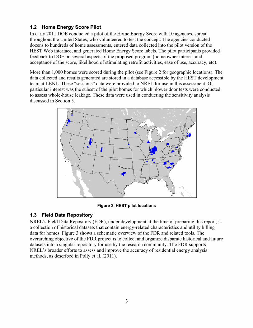
1.2 Home Energy Score Pilot In early 2011 DOE conducted a pilot of the Home Energy Score with 10 agencies, spread throughout the United States, who volunteered to test the concept. The agencies conducted dozens to hundreds of home assessments, entered data collected into the pilot version of the HEST Web interface, and generated Home Energy Score labels. The pilot participants provided feedback to DOE on several aspects of the proposed program (homeowner interest and acceptance of the score, likelihood of stimulating retrofit activities, ease of use, accuracy, etc).

More than 1,000 homes were scored during the pilot (see Figure 2 for geographic locations). The data collected and results generated are stored in a database accessible by the HEST development team at LBNL. These “sessions” data were provided to NREL for use in this assessment. Of particular interest was the subset of the pilot homes for which blower door tests were conducted to assess whole-house leakage. These data were used in conducting the sensitivity analysis discussed in Section 5.

Figure 2. HEST pilot locations

1.3 Field Data Repository NREL’s Field Data Repository (FDR), under development at the time of preparing this report, is a collection of historical datasets that contain energy-related characteristics and utility billing data for homes. Figure 3 shows a schematic overview of the FDR and related tools. The overarching objective of the FDR project is to collect and organize disparate historical and future datasets into a singular repository for use by the research community. The FDR supports NREL’s broader efforts to assess and improve the accuracy of residential energy analysis methods, as described in Polly et al. (2011).

4

Figure 3. Schematic overview of the FDR

NREL’s assessment of HEST largely coincided with the initial development of the FDR. NREL had been collecting historical datasets and was just beginning to organize these into a singular repository, and to build tools to support the application, when the HEST assessment project began. The HEST assessment project was the first application of FDR capabilities. Figure 4 shows the geographic distribution of data in the FDR at the time of its use for this assessment.

Figure 4. Geographic distribution of data in the FDR as of spring 2012

For this project, NREL developed an “interpreter” to map house characteristics data from the FDR to HEST. The interpreter facilitated comparing predicted energy uses from HEST to weather-normalized measured energy uses stored in the FDR.

5

Translating data from the FDR to inputs for a particular energy analysis tool is challenging and can introduce some uncertainty into the process. For example, if energy analysis software offers discrete choices of attic insulation R-value, and none of the choices perfectly match the value in the FDR, some uncertainty is introduced when the interpreter makes the most logical, though imperfect, choice in the software.

The FDR, data sources, and data translation are discussed in more detail in Appendix B.

1.4 Overview of Approach Predicted energy uses from HEST were compared to measured energy uses (i.e., weather-normalized utility billing data). Similarly, predicted energy uses from two other residential energy analysis tools were compared to measured energy uses. The FDR and supporting translation software were used to conduct these comparative analyses. The results of the comparative analyses are presented and discussed in Section 2.

Multivariate linear models of measured energy use and of the residuals between predicted and measured energy uses were developed to examine the impacts of HEST inputs. These models inform potential changes to the software that may improve agreement between predictions and measurements. Results of the statistical modeling are presented in Section 3.

The Home Energy Score assesses the performance of a home’s energy-related assets under typical operating conditions (standard occupants). On the other hand, utility billing data reflect the performance of a home’s energy-related assets under actual operating conditions, which may not be typical. A Monte Carlo uncertainty analysis was conducted to estimate the portion of the total observed variability between predicted and measured energy uses that is explained by variability in occupant operation of the home. This analysis is described in Section 4.

The HEST input structure allows either a qualitative assessment or a quantitative measurement of whole-house air leakage. A question that is important to DOE is whether to require blower door measurement as part of the Home Energy Score assessment process (currently an optional input). Leveraging data collected during the Home Energy Score pilot, NREL examined the sensitivity to using quantitative versus qualitative input in HEST. This analysis is described in Section 5.

Although the focus of this work is HEST, results of the analyses are reported in terms of energy rather than score because the process of translating energy into a score was in flux at the time this report was prepared. Results and discussion of the score as proposed on May 19, 2012 are included in Section 6.

1.5 Limitations of Approach There are a number of limitations to using historical datasets to assess software accuracy:

• The datasets may not be representative of the broader population of homes and assessors (who collect the data). Because the data were not collected as part of designed experiments, no statistical sampling procedures were applied. The “catch-as-catch-can” approach will generally result in data that are not statistically scalable to the broader population.

6

• Historical data were collected for a particular purpose using a specific data collection instrument (e.g., specific rating software). Assessors tend to view a house through the data collection instrument they have been trained to use. Applying data collected for one purpose, at a particular point in time, to other applications is challenging. Significant uncertainty is likely to be introduced when the data are transformed to meet other needs.

• The data collected are generally limited to asset features of the home. Very few operational data are collected. Very little information is collected about atypical energy-using devices (e.g., swimming pools). Measured energy use data (i.e., utility bills) reflect operational variations and atypical energy uses.

1.6 Advantages of Approach Advantages of an automated, empirical data-driven, population-based approach to assessing software accuracy include:

• Comparing predictions of energy uses to measured energy uses helps address skeptics’ concerns that predictions are not accurate. The approach can demonstrate whether software predictions are “right, on average” and provide useful information about level of uncertainty in energy use predictions. Empirically-based testing augments highly detailed software-to-software testing (e.g., BESTEST-EX as described by Judkoff et al. [2010]).

• Using a population of homes in an assessment quantifies uncertainty in predictions across the population and allows stakeholders to assess risks associated with using those predictions.

• Statistical analyses of population data help identify patterns that can be useful in isolating issues that drive errors in predictions. For example, if statistical evaluation of differences between predicted and measured energy use demonstrates that heavily ground-coupled models tend to produce larger average errors, it could indicate a potential issue with ground modeling in the software.

• Automated, data-driven modeling facilitates “what if” analysis. For example, what is the impact of changing standard operational assumptions used in asset assessments? Do answers get “more right, on average?” Such questions can be easily answered programmatically once the framework for running population data through software has been developed.

7

2 Comparison of Predicted Energy Use to Measured Data Data from the FDR were programmatically mapped to three energy analysis tools: HEST, SIMPLE, and REM/Rate. Predicted energy uses from these tools are compared to measured energy uses in the following sections: results from HEST are presented and discussed in Section 2.1, results of the SIMPLE analysis are presented in Section 2.2, results for REM/Rate are presented in Section 2.3, and results for all three tools are summarized in Section 2.4.

Of the 1183 homes in the FDR, some were programmatically excluded for a variety of reasons: missing utility billing data, poor data quality, or presence of (known) asset features that cannot be modeled in the analysis tool.9 The intersection of all the homes successfully simulated in all three analysis tools (859 electric and 500 natural gas [NG]) and the utility bills are compared in the following analysis.

2.1 Scoring Tool Data from the FDR were mapped to the April 27, 2012 release of LBNL’s HEST, submitted to the application programming interface, and the results returned by the application programming interface were collected into a database. The process of mapping FDR data to HEST inputs is detailed in Appendix C.

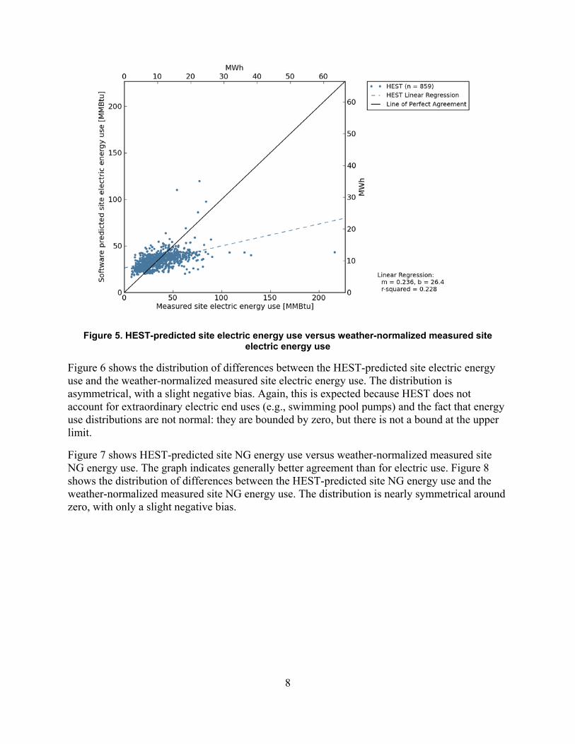
Figure 5 shows HEST-predicted site electric energy use versus weather-normalized measured site electric energy use. In general, HEST tends to underpredict homes with high measured electric energy use and overpredict electric energy use in homes with low measured use. As discussed earlier, HEST models typical occupancy; thus, it would not be expected to respond to unusually low or high energy use. Even if HEST were perfectly accurate, and all the asset-related inputs were perfectly collected and entered into the software, one would not expect the linear regression line to match the line of perfect agreement because actual occupant behavior is not considered when predicting electric energy use for an asset rating. This is true for all the graphical presentations of predicted versus measured energy use (like Figure 5) in this report. The points to the far right of the graph, well below the line of perfect agreement, are likely homes with electrical loads are that are not considered in the asset assessment: swimming pools, hot tubs, aquariums, waterbeds, second refrigerators, etc. Information about these end uses is not available in the FDR.

9 The decision about whether a tool can model a particular house configuration or technology is somewhat subjective. The process of translating the FDR data to software inputs is detailed in Appendix C and Appendix D.

8

Figure 5. HEST-predicted site electric energy use versus weather-normalized measured site electric energy use

Figure 6 shows the distribution of differences between the HEST-predicted site electric energy use and the weather-normalized measured site electric energy use. The distribution is asymmetrical, with a slight negative bias. Again, this is expected because HEST does not account for extraordinary electric end uses (e.g., swimming pool pumps) and the fact that energy use distributions are not normal: they are bounded by zero, but there is not a bound at the upper limit.

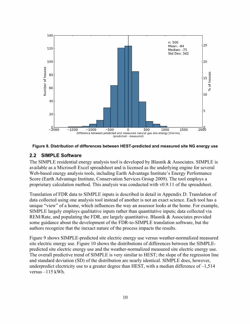
Figure 7 shows HEST-predicted site NG energy use versus weather-normalized measured site NG energy use. The graph indicates generally better agreement than for electric use. Figure 8 shows the distribution of differences between the HEST-predicted site NG energy use and the weather-normalized measured site NG energy use. The distribution is nearly symmetrical around zero, with only a slight negative bias.

9

Figure 6. Distribution of differences between HEST-predicted and measured site electric energy use

Figure 7. HEST-predicted site NG energy use versus weather-normalized measured site NG energy use

10

Figure 8. Distribution of differences between HEST-predicted and measured site NG energy use

2.2 SIMPLE Software The SIMPLE residential energy analysis tool is developed by Blasnik & Associates. SIMPLE is available as a Microsoft Excel spreadsheet and is licensed as the underlying engine for several Web-based energy analysis tools, including Earth Advantage Institute’s Energy Performance Score (Earth Advantage Institute, Conservation Services Group 2009). The tool employs a proprietary calculation method. This analysis was conducted with v0.9.11 of the spreadsheet.

Translation of FDR data to SIMPLE inputs is described in detail in Appendix D. Translation of data collected using one analysis tool instead of another is not an exact science. Each tool has a unique “view” of a home, which influences the way an assessor looks at the home. For example, SIMPLE largely employs qualitative inputs rather than quantitative inputs; data collected via REM/Rate, and populating the FDR, are largely quantitative. Blasnik & Associates provided some guidance about the development of the FDR-to-SIMPLE translation software, but the authors recognize that the inexact nature of the process impacts the results.

Figure 9 shows SIMPLE-predicted site electric energy use versus weather-normalized measured site electric energy use. Figure 10 shows the distributions of differences between the SIMPLE-predicted site electric energy use and the weather-normalized measured site electric energy use. The overall predictive trend of SIMPLE is very similar to HEST; the slope of the regression line and standard deviation (SD) of the distribution are nearly identical. SIMPLE does, however, underpredict electricity use to a greater degree than HEST, with a median difference of –1,514 versus –115 kWh.

11

Figure 9. SIMPLE-predicted site electric energy use versus weather-normalized measured site electric energy use

Figure 10. Distribution of differences between SIMPLE-predicted and measured site electric energy use

12

Figure 11 shows SIMPLE-predicted site NG energy use versus weather-normalized measured site NG energy use. As seen with HEST, SIMPLE was better able to accurately predict NG use than site electricity consumption. Figure 12 shows the distribution of differences between the SIMPLE-predicted site NG energy use versus the weather-normalized measured site NG energy use. SIMPLE predictions of gas use trend with measured values a little better than HEST, with a regression slope closer to unity, and a smaller standard deviation in the distribution of differences. But like the electricity use predictions, SIMPLE tends to underpredict NG use to a greater degree than HEST, with a median difference of –177 versus –76 therms.

Figure 11. SIMPLE-predicted site NG energy use versus weather-normalized measured site NG energy use.

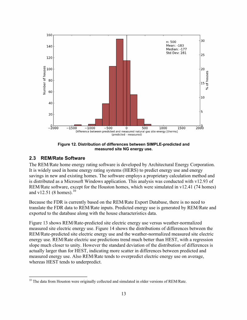
13

Figure 12. Distribution of differences between SIMPLE-predicted and measured site NG energy use.

2.3 REM/Rate Software The REM/Rate home energy rating software is developed by Architectural Energy Corporation. It is widely used in home energy rating systems (HERS) to predict energy use and energy savings in new and existing homes. The software employs a proprietary calculation method and is distributed as a Microsoft Windows application. This analysis was conducted with v12.93 of REM/Rate software, except for the Houston homes, which were simulated in v12.41 (74 homes) and v12.51 (8 homes).10

Because the FDR is currently based on the REM/Rate Export Database, there is no need to translate the FDR data to REM/Rate inputs. Predicted energy use is generated by REM/Rate and exported to the database along with the house characteristics data.

Figure 13 shows REM/Rate-predicted site electric energy use versus weather-normalized measured site electric energy use. Figure 14 shows the distributions of differences between the REM/Rate-predicted site electric energy use and the weather-normalized measured site electric energy use. REM/Rate electric use predictions trend much better than HEST, with a regression slope much closer to unity. However the standard deviation of the distribution of differences is actually larger than for HEST, indicating more scatter in differences between predicted and measured energy use. Also REM/Rate tends to overpredict electric energy use on average, whereas HEST tends to underpredict.

10 The data from Houston were originally collected and simulated in older versions of REM/Rate.

14

Figure 13. REM/Rate-predicted site electric energy use versus weather-normalized measured site electric energy use

Figure 14. Distribution of differences between REM/Rate-predicted and measured site electric energy use

15

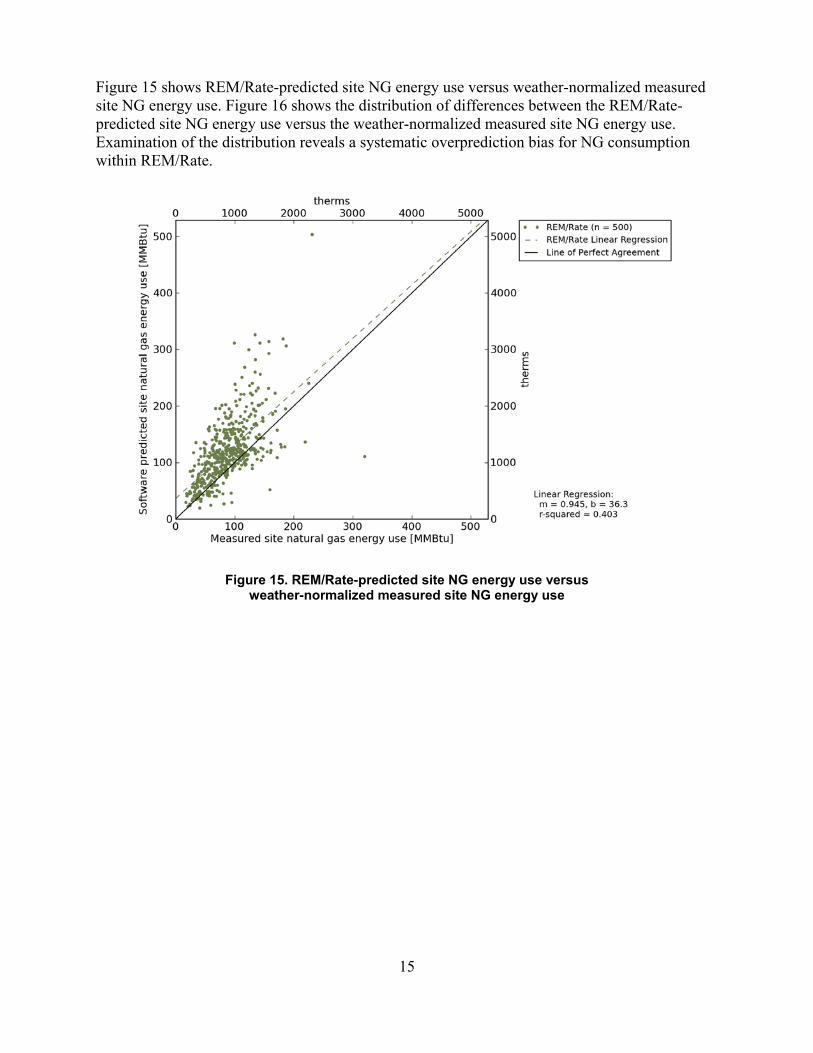
Figure 15 shows REM/Rate-predicted site NG energy use versus weather-normalized measured site NG energy use. Figure 16 shows the distribution of differences between the REM/Rate-predicted site NG energy use versus the weather-normalized measured site NG energy use. Examination of the distribution reveals a systematic overprediction bias for NG consumption within REM/Rate.

Figure 15. REM/Rate-predicted site NG energy use versus weather-normalized measured site NG energy use

16

Figure 16. Distribution of differences between REM/Rate-predicted and measured site NG energy use

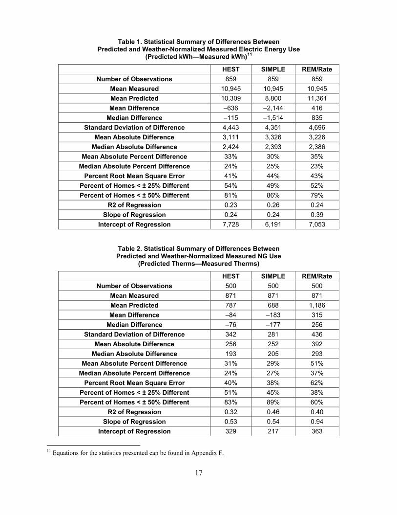
2.4 Summary Table 1 summarizes the differences between predicted and weather-normalized measured electric energy uses for the three analysis tools. Table 2 summarizes the differences between predicted and weather-normalized measured NG use.

Of the tools evaluated, HEST has the smallest median difference between predicted and measured electric energy use: –115 kWh/yr versus –1,514 for SIMPLE and 835 for REM/Rate, though the overall difference in this value between the three tools is small, less than 9%. HEST had the highest percentage of homes with predicted electric energy use within ±25% of the measured electric energy use; 54% of the homes were within this range

The median difference between the NG use predicted by HEST and the measured gas use is –76 therms. This can be compared to –177 therms for SIMPLE and 256 therms for REM/Rate. Of the three tools, HEST had the highest percentage of homes with predicted gas use within ±25% of the measured gas use; 51% of the homes were within this range.

17

Table 1. Statistical Summary of Differences Between Predicted and Weather-Normalized Measured Electric Energy Use

(Predicted kWh—Measured kWh)11

HEST SIMPLE REM/Rate Number of Observations 859 859 859

Mean Measured 10,945 10,945 10,945 Mean Predicted 10,309 8,800 11,361 Mean Difference –636 –2,144 416

Median Difference –115 –1,514 835 Standard Deviation of Difference 4,443 4,351 4,696

Mean Absolute Difference 3,111 3,326 3,226 Median Absolute Difference 2,424 2,393 2,386

Mean Absolute Percent Difference 33% 30% 35% Median Absolute Percent Difference 24% 25% 23%

Percent Root Mean Square Error 41% 44% 43% Percent of Homes < ± 25% Different 54% 49% 52% Percent of Homes < ± 50% Different 81% 86% 79%

R2 of Regression 0.23 0.26 0.24 Slope of Regression 0.24 0.24 0.39

Intercept of Regression 7,728 6,191 7,053

Table 2. Statistical Summary of Differences Between Predicted and Weather-Normalized Measured NG Use

(Predicted Therms—Measured Therms)

HEST SIMPLE REM/Rate Number of Observations 500 500 500

Mean Measured 871 871 871 Mean Predicted 787 688 1,186 Mean Difference –84 –183 315

Median Difference –76 –177 256 Standard Deviation of Difference 342 281 436

Mean Absolute Difference 256 252 392 Median Absolute Difference 193 205 293

Mean Absolute Percent Difference 31% 29% 51% Median Absolute Percent Difference 24% 27% 37%

Percent Root Mean Square Error 40% 38% 62% Percent of Homes < ± 25% Different 51% 45% 38% Percent of Homes < ± 50% Different 83% 89% 60%

R2 of Regression 0.32 0.46 0.40 Slope of Regression 0.53 0.54 0.94

Intercept of Regression 329 217 363

11 Equations for the statistics presented can be found in Appendix F.

18

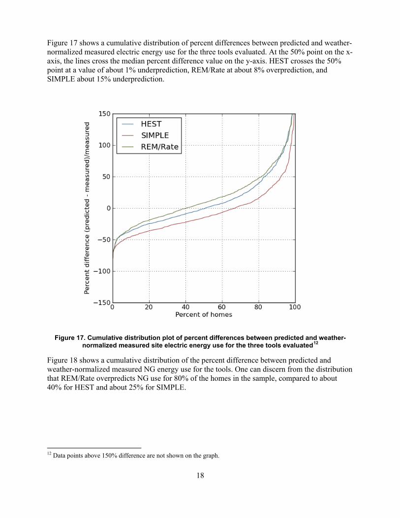
Figure 17 shows a cumulative distribution of percent differences between predicted and weather-normalized measured electric energy use for the three tools evaluated. At the 50% point on the x-axis, the lines cross the median percent difference value on the y-axis. HEST crosses the 50% point at a value of about 1% underprediction, REM/Rate at about 8% overprediction, and SIMPLE about 15% underprediction.

Figure 17. Cumulative distribution plot of percent differences between predicted and weather-normalized measured site electric energy use for the three tools evaluated12

Figure 18 shows a cumulative distribution of the percent difference between predicted and weather-normalized measured NG energy use for the tools. One can discern from the distribution that REM/Rate overpredicts NG use for 80% of the homes in the sample, compared to about 40% for HEST and about 25% for SIMPLE.

12 Data points above 150% difference are not shown on the graph.

19

Figure 18. Cumulative distribution plot of percent differences between predicted and

weather-normalized measured site NG energy use for the three tools evaluated13

13 Data points above 150% difference are not shown on the graph.

20

3 Statistical Models To estimate which inputs contribute the most to differences between HEST predictions and measured energy uses, a statistical analysis approach was applied to the FDR records. More specifically, multiple linear regression (MLR) was used to develop empirical models from HEST inputs and utility billing data. This section covers the approach taken, the resulting models, and what can be concluded from these models.

3.1 Approach The general model equation for MLR is as follows:

y = β0 + β1x1 + β2x2 + … + βnxn + ε

where,

y is the dependent variable

β0 is the intercept

β1 through βn are the coefficients

x1 through xn are the independent variables (inputs)

ε is the remaining error.

In MLR, a least-squares-fit algorithm is applied to a dataset that contains multiple records with each record containing one y-value and its associated x-values. Most statistical software programs calculate the coefficients and probability values that allow one to evaluate which coefficients are significant. Polynomial terms (i.e., xn

2) and interaction terms (i.e., x1x2) are sometimes included in the model if they improve the overall fit and have minimal correlation with the other independent variables. Although one starts out initially with a model containing practically all possible independent variables, common practice is to eliminate insignificant variables until a “reduced” model containing only significant variables is achieved.

3.2 Home Energy Score Test Dependent Variables and Inputs For evaluating HEST results, the following dependent variables were used in four separate empirical models:

• Measured site electricity (weather-normalized)

• Measured site NG (weather-normalized)

• Difference site electricity = (predicted site electricity) – (measured site electricity)

• Difference site NG = (predicted site NG) – (measured site NG).

Separate models for measured site electricity and measured site NG were created to estimate which inputs correlate with measured at a significant level and to evaluate how much variability in the measured results can be explained by these inputs. The next step was to model differences between HEST predictions and measured energy uses. Again, separate models were created for site electricity and site NG. The coefficients from these difference models can be examined to

21

evaluate which HEST inputs correlate with increasing or decreasing difference from measured energy use.

There are approximately 40 HEST inputs. Some, such as floor area, are numeric, but many use DOE-2 codes to describe various types of building construction components (tables for these codes can be found at https://sites.google.com/a/lbl.gov/hes-public/calculation-methodology/appendices/appendix-e). There are separate codes for skylight types, wall types, roof types, foundation types, and many other components that make up a building. For statistical analysis, the frequency of each specific code was examined and then a binary variable was defined for each. More details about variable coding for statistical analysis are given in Section 3.4. An example of a DOE-2 ceiling construction code is “ecwf30,” which is defined as 3.5-in. wood ceiling joists @ 24 in. on center (o.c.), 10.5-in. (R-30) fiberglass fill ceiling insulation, and 0.5-in. gypsum wallboard. These construction codes were used in the variable names to allow lookup in the DOE-2 tables for further details. It was desirable to extract insulation R-values from these construction codes because insulation R-values can be treated as numeric variables that likely correlate directly with energy use. For the variable RoofRValue, the R-values were extracted from both “roof” construction codes and “ceiling” construction codes, because often a building had insulation listed for one but not for the other.

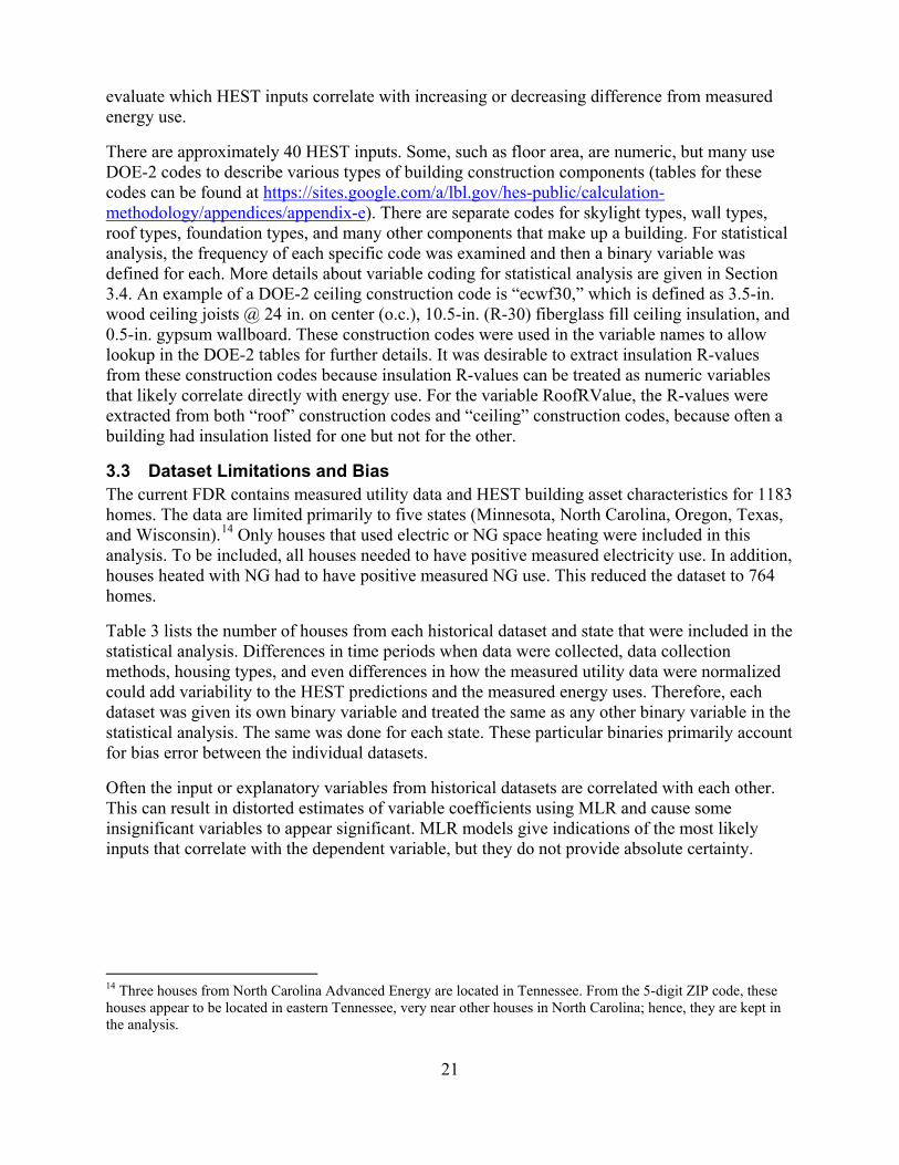
3.3 Dataset Limitations and Bias The current FDR contains measured utility data and HEST building asset characteristics for 1183 homes. The data are limited primarily to five states (Minnesota, North Carolina, Oregon, Texas, and Wisconsin).14 Only houses that used electric or NG space heating were included in this analysis. To be included, all houses needed to have positive measured electricity use. In addition, houses heated with NG had to have positive measured NG use. This reduced the dataset to 764 homes.

Table 3 lists the number of houses from each historical dataset and state that were included in the statistical analysis. Differences in time periods when data were collected, data collection methods, housing types, and even differences in how the measured utility data were normalized could add variability to the HEST predictions and the measured energy uses. Therefore, each dataset was given its own binary variable and treated the same as any other binary variable in the statistical analysis. The same was done for each state. These particular binaries primarily account for bias error between the individual datasets.

Often the input or explanatory variables from historical datasets are correlated with each other. This can result in distorted estimates of variable coefficients using MLR and cause some insignificant variables to appear significant. MLR models give indications of the most likely inputs that correlate with the dependent variable, but they do not provide absolute certainty.

14 Three houses from North Carolina Advanced Energy are located in Tennessee. From the 5-digit ZIP code, these houses appear to be located in eastern Tennessee, very near other houses in North Carolina; hence, they are kept in the analysis.

22

Table 3. Home Count by Historical Datasets and State

Data Set Description15 Total Count State Building America Audit Assessment 48 Minnesota

EPA ENERGY STAR® Qualified Homes Study 73 Minnesota EPA ENERGY STAR Qualified Homes Study 1 Wisconsin

Advanced Energy System Vision 255 North Carolina Advanced Energy System Vision 3 Tennessee

Oregon EPS Study 172 Oregon Houston Utility Study 42 Texas

Wisconsin Housing Study 170 Wisconsin

In addition to HEST inputs, climate differences are believed to be important. To capture actual climatic differences, two additional independent variables, heating degree days (HDDs) (base 65°F) and cooling degree days (CDDs) (base 65°F), were joined to the dataset and treated as numeric variables. Values for these variables were taken from Typical Meteorological Year (TMY) weather files at weather stations near home locations (based on ZIP code values).

3.4 Variable Coding All original HEST inputs were coded. These coded inputs became the independent variables in the regression models. Independent variables were coded primarily to allow more meaningful comparison of the coefficients in the final models. The actual coding method depended on whether the variable was numeric or binary. Unless otherwise noted, the numeric variables were coded using a univariate method. Univariate coding is done by subtracting the variable mean and then dividing this difference by the variable standard deviation. The resulting coded variable has a variance of one, hence the term univariate. In the few cases where the variable distribution was highly skewed toward zero and the ratio of mean to standard deviation was <1, an alternate coding was used. For the alternate coding, the 95th percentile of the variable was defined as 1 and zero was defined as –1.

With the exception of hot water fuel (hwFuel), the binary variables were coded as Yes = 1 and No = 0. Hot water fuel was coded as Gas = 1 and Electric = –1 to test a possible interaction with the hot water energy factor (hwEnergyFactor). In most cases, the number 1 (or Yes) implies that the particular building has the HEST input characteristic. For example, C_HT_EFN = 1, means the heating type is an electric furnace. Although this is a generally accepted statistical modeling practice, the binary coded variables often have larger coefficients than a univariate coded variable with the same confidence level (CL) as a result of the coding technique. Hence, other statistics from the MLR analysis should be examined to evaluate which variables are most significant.

The binary coding created multiple variables for each categorical input. For example, there were six heating system type categories (electric and NG only). Standard practice is to choose one category as a control. The control has no further variable assignment, as all other categories are

15 Further description of these datasets can be found in Appendix B.

23

referenced to the control. New binary variables are created for each of the other categories. Table 4 demonstrates this method for heating types where “gas furnace” is chosen as the control. Not every binary variable is used in the final model, as most do not vary significantly from the control. The resulting number of total variables slightly exceeded 100 (HEST plus state binaries and dataset binaries). A complete list of HEST variables with descriptions is included in Appendix C.

Table 4. Example of Binary Coding for Heating Type Category HEST Input

Heating Type Description Record

Count C_HT_EBB C_HT_EFN C_HT_EHP C_HT_GBL C_HT_GWF

gfn (control) Gas furnace 471 0 0 0 0 0

ebb Electric baseboard 10 1 0 0 0 0

efn Electric furnace 3 0 1 0 0 0

ehp Electric heat pump 246 0 0 1 0 0

gbl Gas boiler 27 0 0 0 1 0

gwf Gas wall furnace 7 0 0 0 0 1

3.5 Models of Measured Energy Use Approximately 75% of the observations were randomly selected as a model set; the remaining observations were kept as a test set. The model set was used to build the model. The MLR model was then applied to the test set to predict the measured energy use. The R-squared value estimated from the test set (plot of measured versus MLR predicted) can be compared to the R-squared value from the model building process. The R-squared value from the test set does not have to be exactly the same as the R-squared value from the model set, but should be comparable.16

Table 5 shows the resulting MLR model with measured site electricity as the dependent variable. All variables listed are significant at a CL ≥95%. The variables highlighted in yellow are significant at a CL >99%. The list is divided between numeric variables and binary and sorted from most significant to least significant within each variable type. An adjusted R-squared value of 0.433 resulted; this implies that the model can explain approximately 43% of the observed variability in measured electricity use.

16 There are no specific rules, but from experience, if the adjusted R-squared value for the model set exceeds the adjusted R-squared value for the test set by more than 0.1, the model set has likely not captured the most significant factors.

24

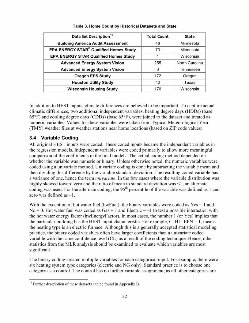
Table 5. Significant Model Variables and Coefficients for Measured Site Electricity

Variable Type Model Variable Original Variable Description Coefficients

(MMBtu) CL

From MLR

(Intercept)

32.4 100.0%

Numeric C_numberBedrooms Number of bedrooms 3.8 100.0% Numeric C_floorArea Floor area (ft2) 5.2 100.0% Numeric C_W_WindowArea Western facing window area (ft2) 1.4 98.5% Binary C_HT_EHP Heating type EHP (electric heat pump) 17.5 100.0% Binary C_HT_EBB Heating type EBB (electric baseboard) 25.2 100.0% Binary C_HT_EFN Heating type EFN (electric furnace) 41.7 100.0% Binary State_MN State of Minnesota –6.3 100.0% Binary C_hwFuel Hot water fuel type (gas or electric) –3.4 100.0%

Binary C_WC_ewps19wo

Wall construction code ewps19wo (0.5-in lapped wood siding, 0.5-in

fiberboard sheathing, 5.5-in. wood studs @ 16 in. o.c., 1-in. expanded polystyrene, R-19 mineral fiber batt

insulation, 0.5-in. gypsum wallboard)

–7.7 98.2%

Figure 19 shows a graph of the measured site electricity for the model set versus the MLR prediction and a graph of the test set where the resulting MLR model is used to make predictions. When linear regression is applied on the measured site electricity versus the MLR predicted site electricity for the test set, an adjusted R-squared value of 0.343 results. The test set results in an adjusted R-square that is comparable to the model adjusted R-square and the plot of measured energy use from the test set has a pattern similar to the plot of measured from the model set, confirming the MLR model’s predictive capability for this dataset. The coefficients will likely change as more data become available in the FDR. Nevertheless, the most significant coefficients appear to be understandable. For example, increased electricity use with increased number of bedrooms is indicated in the model and might be due to more occupants using more electricity. A positive coefficient for floor area might follow from similar factors. Using gas for hot water fuel should decrease electricity use, hence the negative coefficient. Increased electricity use is expected when electric baseboard, electric furnace, or electric heat pump are used.

25

Figure 19. Measured versus MLR-predicted site electricity for the model set (left) and test set (right)

Minnesota appears to have significantly lower electricity use than other states in the dataset. Both Minnesota datasets showed similar bias. Because of the limited number of datasets, one cannot conclude at this time that Minnesota is truly different. The Minnesota variable correlates strongly (R values greater than 0.5) with both ceiling construction using R-49 insulation and wall construction using R-19 insulation. The same level of correlation for these inputs was not observed for other states. As data are collected for Minnesota homes with less insulation, these construction inputs may become significant.

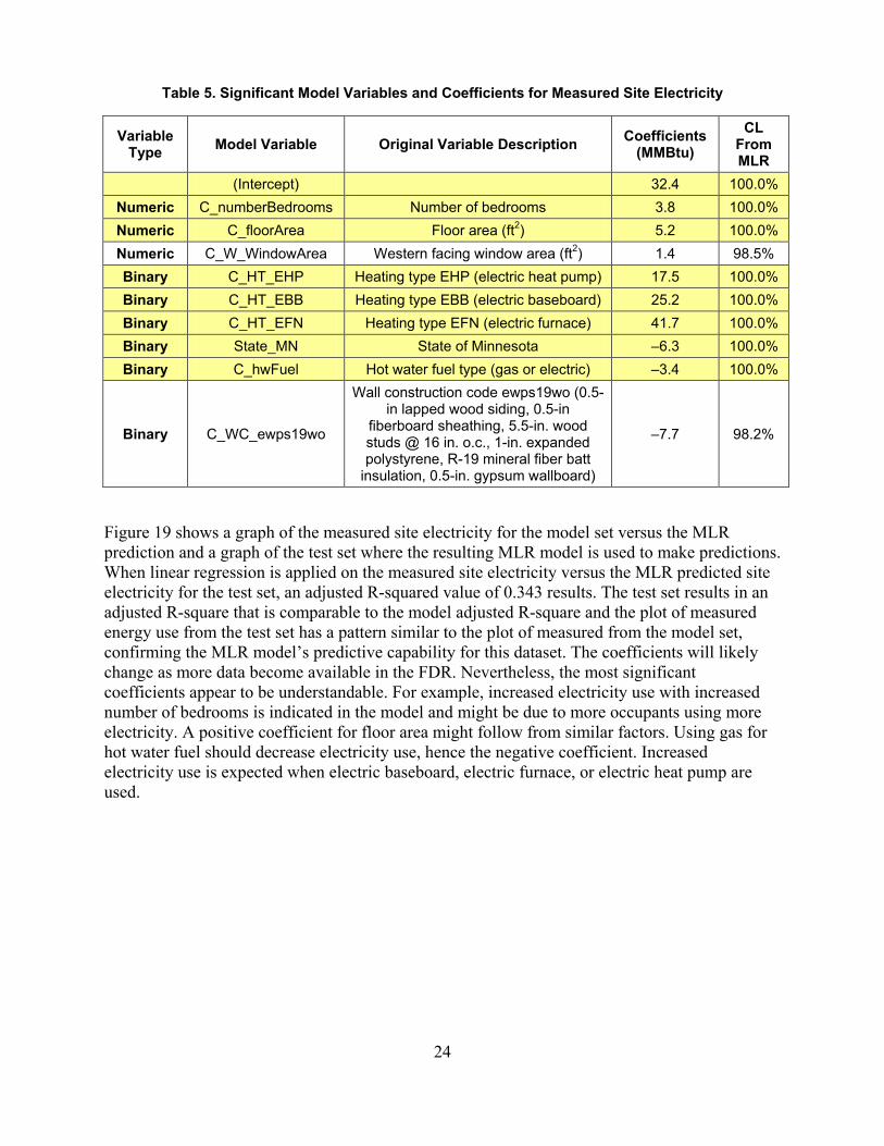
For modeling measured site NG, only buildings where NG is used for space heating were included. This reduced the number of observations to 505. As with the electric model, these observations were further divided into a model set (about 75% randomly selected) and a test set (the remainder).

Table 6 shows the resulting MLR model with measured site NG as the dependent variable. The resulting adjusted R-squared for this model is 0.650, which indicates that the model explains 65% of the variability. Graphs in Figure 20 show measured site NG versus MLR-predicted site NG, with the test set graph showing a pattern similar to the model set graph. At least some of the model variable coefficients appear to agree with how the input might be expected to influence NG use. For example, houses in locations with more HDDs would be expected to use more NG for space heating. Increased air leakage and increased floor area both contribute to higher NG use. A gas furnace with higher efficiency reduces NG use. Some variables do not make sense and may be artifacts of the current available data. In particular, age in years indicates a reduction in NG use for older buildings. Age in years correlates strongly with the Oregon dataset. As older

0 20 40 60 80

020

4060

8010

012

0

Model Set

MLR Predicted Site Electrici

Mea

sure

d S

ite E

lect

ricity

(MM

Btu

0 20 40 60 80

020

4060

8010

012

0

Test Set

MLR Predicted Site Electrici M

easu

red

Site

Ele

ctric

ity (M

MB

tu

26

homes in other states are added to the FDR, a better test should result for the age in years variable.

Table 6. Significant Model Variables and Coefficients for Measured Site NG

Variable Type Model Variable Original Variable Description Coefficients

(MMBtu) CL

from MLR

(Intercept)

78.1 100.0%

Numeric C_HDD_65F HDDs (base 65°F) 20.8 100.0% Numeric C_airLeakage50ip Air leakage (cfm) 8.8 100.0%

Numeric C_heatingEfficiency Heating efficiency for home heating system –24.9 100.0%

Numeric C_floorArea Floor area (ft2) 7.0 100.0% Numeric C_E_WindowArea Eastern facing window area (ft2) 5.1 99.9% Numeric C_age_years House age in years –5.9 99.9% Numeric C_N_WindowArea Northern facing window area (ft2) 4.3 99.7%

Numeric C_WASG_Total sum((Window area) × (solar heat gain coefficient [SHGC])) 5.5 99.3%

Numeric C_houseOrientation House orientation (0 = N, 90 = E, 180 = S, and 270 = W) –3.8 98.9%

Binary C_hwFuel Hot water fuel type (gas or electric) 8.7 100.0%

Binary C_FC_efwf30ca

Floor construction code efwf30ca (11.5-in wood joists @ 24 in. o.c., R-30 mineral

fiber batt insulation, 0.75-in. wood underlayment, 0.75-in. wood subfloor,

carpeting)

–39.7 99.7%

Binary C_FC_efwf25ca

Floor construction code efwf30ca (11.5-in. wood joists @ 24 in. o.c., R-25 mineral

fiber batt insulation, 0.75-in. wood underlayment, 0.75-in. wood subfloor,

carpeting)

–16.1 99.7%

27

Figure 20. Measured versus MLR-predicted site NG for model set (left) and test set (right)

3.6 Models of Differences Between Predicted and Measured Energy Uses Table 7 shows the resulting MLR model with difference site electricity as the dependent variable. Again, the difference is predicted site electricity minus measured site electricity. The resulting adjusted R-squared value for this model is 0.199, which indicates that only about 20% of the variability in the differences can be explained by this model. Seven variables listed are significant at CLs ≥ 99% and three other variables are significant at 95% CL. Additional validation was done by combining the MLR prediction for measured site electricity with the MLR prediction for the difference model. Plotting the combined MLR prediction versus the measured site electricity shows a pattern very similar to the HEST predictions (see Appendix E).

0 50 100 150 200

050

100

150

200

Model Set

MLR Predicted Site Natural G

Mea

sure

d S

ite N

atur

al G

as (M

MB

0 50 100 150 200

050

100

150

200

Test Set

MLR Predicted Site Natural G M

easu

red

Site

Nat

ural

Gas

(MM

B

28

Table 7. Significant Model Variables and Coefficients for Difference Site Electricity

Variable Type Model Variable Original Variable Description Coefficients

(MMBtu) CL from

MLR (Intercept) –1.2 85.5% Numeric C_numberBedrooms Number of bedrooms –3.3 100.0% Numeric C_floorArea Floor area (ft2) 2.4 99.7%

Numeric C_WallRValue Wall R-value determined from wall construction inputs –1.7 99.6%

Binary C_HT_EFN Heating type EFN (electric furnace) 26.9 100.0% Binary C_CT_ehp Cooling type ehp (electric heat pump) –5.1 99.9%

Binary C_ST_dseab

Skylight type dseab (double-pane, low-solar-gain low-E (e = 0.05 on surface 2, aluminum spacer and frame with thermal break)

–18.4 99.5%

Binary State_MN State of Minnesota 4.7 99.5%

Binary C_WC_ewps19wo

Wall construction code ewps19wo (0.5-in. lapped wood siding, 0.5-in. fiberboard sheathing, 5.5-in. wood studs @ 16 in. o.c., 1-in. expanded polystyrene, R-19 mineral fiber batt insulation, 0.5-in. gypsum wallboard)

9.1 98.9%

Binary C_HT_EBB Heating type EBB (electric baseboard) 9.6 97.1%

Binary C_CC_ecwf21

Ceiling construction code ecwf21 (3.5-in. wood ceiling joists @ 25 in. o.c., R-21 fiberglass fill ceiling insulation, 0.5-in. gypsum wallboard)

8.1 96.7%

The coefficients give a magnitude estimate and sign for each variable. The very low R-squared values indicate that only a fraction of the difference between HEST-predicted and measured values can be explained by the inputs. Nevertheless, a few variables might be worth investigating. At least six of the significant variables in the difference site electricity model occur in the measured site electricity model. The negative coefficients for number of bedrooms, wall R-value, and a few other variables indicate that the difference decreases as these variables increase. The positive coefficients for variables such as floor area, electric furnace, and the R-19 wall construction indicate that the difference increases as these variables increase.

Table 8 shows the resulting MLR model with difference site NG as the dependent variable. The resulting adjusted R-squared value for this model is 0.456, which indicates that about 46% of the variability in the difference can be explained by this model. All variables listed are significant at a CL ≥ 95%. Seven numeric variables plus three binary variables are significant at a CL > 99%.

29

Table 8. Significant Model Variables and Coefficients for Difference Site NG

Variable Type Model Variable Original Variable Description Coefficients

(MMBtu) CL from

MLR (Intercept) 9.8 97.7% Numeric C_HDD_65F HDDs (base 65°F) 7.5 100.0%

Numeric C_E_WASG (East window area) × (SHGC) –6.7 100.0%

Numeric C_heatingEfficiency Heating efficiency for home heating system –23.8 100.0%

Numeric C_RoofRValue Roof R-value determined from roof

construction and ceiling construction inputs

–5.5 100.0%

Numeric C_N_WindowArea North-facing window area (ft2) –4.2 99.8%

Numeric C_houseOrientation House orientation (0 = N, 90 = E, 180 = S, and 270 = W) 4.5 99.7%

Numeric C_airLeakage50ip Air leakage (cfm) 4.4 99.4% Numeric C_age_years House age in years 4.3 97.4%

Binary C_WC_ewwf00wo

Wall construction code ewwf00wo (0.5-in. lapped wood siding, 0.5-in.

fiberboard sheathing, 3.5-in. wood studs @ 16 in. o.c., 3.5-in. vertical air spaces

(no insulation), 0.5-in. gypsum wallboard)

16.9 100.0%

Binary C_HT_GBL Heating type GBL (gas boiler) 26.6 100.0%

Binary C_WC_ewwf19wo

Wall construction code ewwf19wo (0.5-in. lapped wood siding, 0.5-in.

fiberboard sheathing, 5.5-in. wood studs @ 16 in. o.c., R-19 mineral fiber batt insulation, 0.5-in. gypsum wallboard)

–13.5 99.7%

HDDs were significant for both the measured site NG and the difference model. Both had positive coefficients. The indication is that HEST overpredicts the impact of greater HDDs, perhaps for a variety of reasons: the assumed heating set point may be too high, the variation in indoor air temperature is too great, empty wall cavities are imperfectly modeled, etc. Air leakage also had positive coefficients for both models. Increased air leakage increases energy use, but HEST might be overpredicting the impact.

Heating efficiency was significant for both the measured site NG and the difference model, but had negative coefficients. The measured site NG model shows a reasonable trend, declining NG use as the heating system efficiency increases. The negative estimate for the difference model indicates that HEST may not completely capture the impact of increasing system efficiency.

The roof R-value was not significant in the measured site NG model, but is significant in the difference model. One would expect that as roof R-value increases, the NG use should decrease, but it might be that in actuality NG use does not decrease as much as HEST predicts. Hence the predicted would be less than the measured.

30

A few other variables had interesting trends. Increased age in years showed lower NG use. The difference model indicated a possible overprediction by HEST. This might be an artifact of limited data. One generally expects newer homes to use less energy, but on average the newer homes have more floor area. Increasing north- and east-facing window area correlates with increasing NG use. The difference model indicated underprediction by HEST for at least the north-facing window area. House orientation indicated lower NG use as the orientation moved away from being directly north (0 angle). The difference model indicated a possible overprediction by HEST for orientation.

The binary variables are sometimes more difficult to explain. The difference model indicates that HEST overpredicted NG use for homes with wood frame wall construction with no insulation (ewwf00wo). This could be due to lower average indoor temperatures caused by zoning or inaccurate modeling of uninsulated walls. One would expect higher energy use with less wall insulation, but in this case the correlation with wall construction types with low insulation did not prove significant in the measured NG model and might be hidden due to other sources of variability. Wall R-values were also estimated based on the DOE-2 wall construction codes and tested separately, but did not prove to be significant. Two floor construction types with R-30 and R-25 insulation (efwf30ca and efwf25ca) correlated with reduction in measured NG use. Lower differences were observed for homes with another type of wall construction (ewwf19wo designates wood frame construction with R-19 mineral fiber batt insulation in the wall).

3.7 Summary In spite of the data limitations, MLR models indicated significant correlations between measured energy use and several HEST inputs. These methods also indicated significant correlations between differences (HEST predicted minus measured energy use) and several HEST inputs. How these inputs were collected and used in the HEST prediction models can be investigated to identify causes for differences from measured energy use and potential improvements to software inputs and models.

The statistical models discussed in this section apply only to the current FDR data used to develop the models. As more data are collected, it is likely that the coefficients will change, new inputs will become significant, and current significant inputs might prove to be insignificant. Nevertheless, the current statistical models identified several HEST inputs that significantly correlated to measured site energy use (both electricity and NG). The difference models identified HEST inputs that correlated with increasing or decreasing difference from measured energy use. These inputs might be causing the differences or they might be used in models or algorithms that are causing the differences.

31

4 Operational Uncertainty Analysis The Home Energy Score assesses the performance of the energy-related assets of a home under typical operating conditions (standard occupants). However, utility billing data reflect the performance of the energy-related assets of a home under actual operating conditions, which can vary greatly. Therefore, when assuming standard occupancy, there is considerable uncertainty that predictions will agree with utility billing data because actual occupant behavior is not considered. The goal of this analysis was to estimate the effect of operational input uncertainty on the uncertainty in energy use predictions. A development version of BEopt™/EnergyPlus17 was used to perform the simulations.

4.1 Approach Two prototypical houses were utilized in the analysis:18

• House A: 1,539-ft2, one-story, detached, inefficient home, representative of 1960s-era construction.

• House B: 2,500-ft2, two-story, detached, more efficient home, representative of new construction.

The following technical approach was used to estimate the effect of operational input uncertainty on the uncertainty in energy use predictions:

1. Identify operational inputs accessible in the BEopt input file and select a subset of key inputs for variation.

2. Define probability distributions representing the uncertainty ranges for each key input.

3. Randomly select values from probability distributions for each key input and simulate energy use for that realization of inputs.

4. Repeat Step 3 for many realizations to generate a range of simulation output.

5. Analyze the distributions of simulated energy uses.

Nineteen inputs related to the operation of the homes were selected for this analysis. These inputs, their physical units, and key notes are listed in Table 9.

.

17The BEopt (Building Energy Optimization) software was developed by NREL to evaluate residential building designs. The software can be used to analyze both new construction and existing home retrofits, and provides detailed analysis using house characteristics. The version of BEopt used in this analysis utilizes the EnergyPlus building energy simulation engine. EnergyPlus has been developed and supported by DOE Building Technologies Program since 1996. 18 More information about the operational uncertainty analysis and assumed features of the homes can be found in Polly (2011).

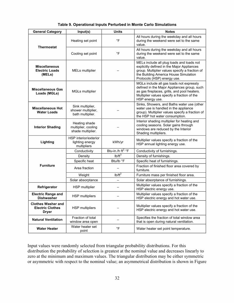
32

Table 9. Operational Inputs Perturbed in Monte Carlo Simulations

General Category Input(s) Units Notes

Thermostat

Heating set point °F All hours during the weekday and all hours during the weekend were set to the same value.

Cooling set point °F All hours during the weekday and all hours during the weekend were set to the same value.

Miscellaneous Electric Loads

(MELs) MELs multiplier –

MELs include all plug loads and loads not explicitly defined in the Major Appliances group. Multiplier values specify a fraction of the Building America House Simulation Protocols (HSP) energy use.

Miscellaneous Gas Loads (MGLs) MGLs multiplier

MGLs include all gas loads not expressly defined in the Major Appliances group, such as gas fireplaces, grills, and pool heaters. Multiplier values specify a fraction of the HSP energy use.

Miscellaneous Hot Water Loads

Sink multiplier, shower multiplier,

bath multiplier. –

Sinks, Showers, and Baths water use (other water use is handled in the appliance group). Multiplier values specify a fraction of the HSP hot water consumption.

Interior Shading Heating shade

multiplier, cooling shade multiplier.

–

Interior shading multiplier for heating and cooling seasons. Solar gains through windows are reduced by the Interior Shading multipliers.

Lighting HSP interior/exterior

lighting energy multipliers

kWh/yr Multiplier values specify a fraction of the HSP annual lighting energy use.

Furniture

Conductivity Btu-in./h·ft2·°F Conductivity of furnishings. Density lb/ft3 Density of furnishings.

Specific heat Btu/lb·°F Specific heat of furnishings.

Area fraction – Fraction of finished floor area covered by furniture.

Weight lb/ft2 Furniture mass per finished floor area. Solar absorptance – Solar absorptance of furnishings.

Refrigerator HSP multiplier – Multiplier values specify a fraction of the HSP electric energy use.

Electric Range and Dishwasher HSP multipliers – Multiplier values specify a fraction of the

HSP electric energy and hot water use.

Clothes Washer and Electric Clothes

Dryer HSP multipliers – Multiplier values specify a fraction of the

HSP electric energy and hot water use.

Natural Ventilation Fraction of total window area open – Specifies the fraction of total window area

that is open during natural ventilation.

Water Heater Water heater set point °F Water heater set point temperature.

Input values were randomly selected from triangular probability distributions. For this distribution the probability of selection is greatest at the nominal value and decreases linearly to zero at the minimum and maximum values. The triangular distribution may be either symmetric or asymmetric with respect to the nominal value; an asymmetrical distribution is shown in Figure

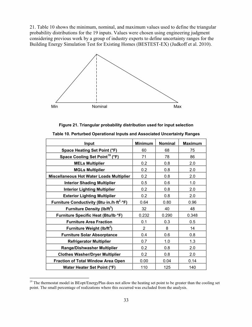
33

21. Table 10 shows the minimum, nominal, and maximum values used to define the triangular probability distributions for the 19 inputs. Values were chosen using engineering judgment considering previous work by a group of industry experts to define uncertainty ranges for the Building Energy Simulation Test for Existing Homes (BESTEST-EX) (Judkoff et al. 2010).

Figure 21. Triangular probability distribution used for input selection

Table 10. Perturbed Operational Inputs and Associated Uncertainty Ranges

Input Minimum Nominal Maximum Space Heating Set Point (°F) 60 68 75

Space Cooling Set Point19 (°F) 71 78 86 MELs Multiplier 0.2 0.8 2.0 MGLs Multiplier 0.2 0.8 2.0

Miscellaneous Hot Water Loads Multiplier 0.2 0.8 2.0 Interior Shading Multiplier 0.5 0.6 1.0 Interior Lighting Multiplier 0.2 0.8 2.0 Exterior Lighting Multiplier 0.2 0.8 2.0

Furniture Conductivity (Btu·in./h·ft2·°F) 0.64 0.80 0.96 Furniture Density (lb/ft3) 32 40 48

Furniture Specific Heat (Btu/lb·°F) 0.232 0.290 0.348 Furniture Area Fraction 0.1 0.3 0.5 Furniture Weight (lb/ft2) 2 8 14

Furniture Solar Absorptance 0.4 0.6 0.8 Refrigerator Multiplier 0.7 1.0 1.3

Range/Dishwasher Multiplier 0.2 0.8 2.0 Clothes Washer/Dryer Multiplier 0.2 0.8 2.0

Fraction of Total Window Area Open 0.00 0.04 0.14 Water Heater Set Point (°F) 110 125 140

19 The thermostat model in BEopt/EnergyPlus does not allow the heating set point to be greater than the cooling set point. The small percentage of realizations where this occurred was excluded from the analysis.

Min Nominal Max

34

4.2 Results For this analysis, approximately 2500 realizations of inputs values were randomly selected and simulated in BEopt/EnergyPlus for both House A and House B. Figure 22 shows annual total source energy use output distributions in Chicago, Illinois for House A and House B. The dashed lines are normal distributions based on the output sample mean and sample standard deviation. For both House A and House B, the SD is equal to approximately 11% of the mean (i.e., the coefficient of variation (COV) = SD/Mean = 0.11).

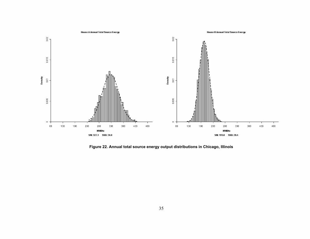
35

Figure 22. Annual total source energy output distributions in Chicago, Illinois

36

Similar uncertainty analyses were undertaken for other U.S. cities as shown in Table 11. Three key takeaways are:

• The COV varies by 0.03 or less between the prototypical houses.

• The COV varies by 0.07 or less (House A) and 0.05 or less (House B) across climates—occupants seem to have greater impact on the total energy use of the homes in milder climates.

• Overall, the analysis shows that even if all other sources of inaccuracy are eliminated in an asset analysis, differences between software predictions and measured source energy could be significant because occupant behavior is variable relative to standard assumptions. For example, simulations showed total source energy use differences of up to 36%.20

Table 11. Mean, SD, and COV for Total Source Energy Use (MMBtu/yr) by Climate

HOUSE A HOUSE B MEAN SD COV MEAN SD COV

Atlanta, Georgia 212.2 27.4 0.13 146.5 19.8 0.14 Chicago, Illinois 327.1 34.8 0.11 193.8 20.4 0.11 Houston, Texas 192.5 26.8 0.14 142.9 21.2 0.15

Los Angeles, California 129.5 22.9 0.18 111.4 18.1 0.16 Phoenix, Arizona 228.7 30.5 0.13 157.6 22.4 0.14

Seattle, Washington 233.6 37.5 0.16 148.7 19.4 0.13 City Average 220.6 30.0 0.14 150.1 20.2 0.14

4.3 Applying Uncertainty Analysis Results to FDR Comparisons Figure 23 compares the results of the operational uncertainty analysis to the results from the HEST comparative analyses in Section 3.1. The gray distribution shows the differences between HEST predictions and measured energy uses in the FDR.21 These differences are the result of all sources of inaccuracy, including inaccuracies in inputs related to the occupants, the asset, and the site. The overlaid blue distribution represents the predicted differences caused by occupant variability relative to standard assumptions.22 The assumption of standard occupancy is necessary to provide an assessment of the home’s energy performance that can be fairly compared to assessments of the energy performance of other homes under the same standard conditions. As seen in Figure 23, occupant variability is a very significant source of inaccuracy, but does not explain all of the differences observed in the FDR comparisons. The remaining sources of inaccuracy could be targeted to improve HEST. For example, assessment procedures

20 The 36% value corresponds to two standard deviations in the Los Angeles climate and roughly bounds 95% of the differences. 21 The comparative analyses in Section 3.1 cover site electricity and natural gas. Total source energy use differences are discussed in Section 6.2. 22 A COV value of 0.14 was used generate occupant variability plot. To simplify the presentation, differences are shifted so the mean difference is zero for each distribution.

37

may be adjusted considering tradeoffs in accuracy, cost, and time necessary to perform the assessment.

Figure 23. Predicted differences due to operational uncertainty overlaid on observed differences from FDR comparisons

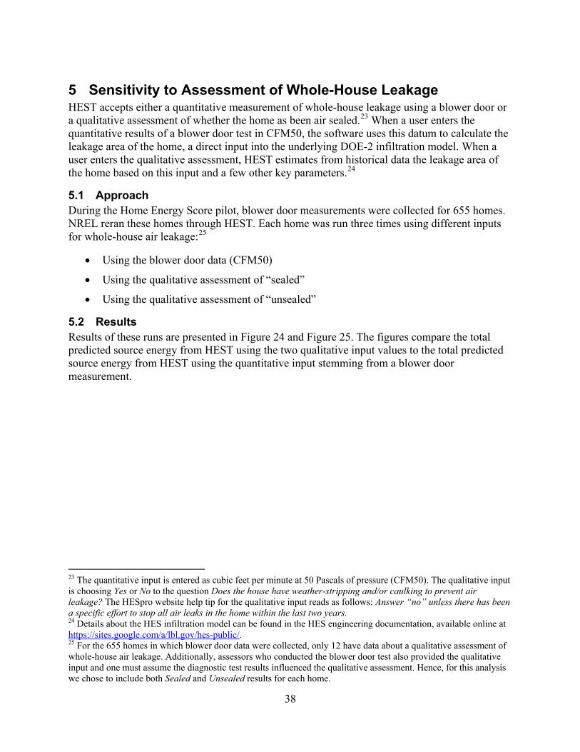
38

5 Sensitivity to Assessment of Whole-House Leakage HEST accepts either a quantitative measurement of whole-house leakage using a blower door or a qualitative assessment of whether the home as been air sealed.23 When a user enters the quantitative results of a blower door test in CFM50, the software uses this datum to calculate the leakage area of the home, a direct input into the underlying DOE-2 infiltration model. When a user enters the qualitative assessment, HEST estimates from historical data the leakage area of the home based on this input and a few other key parameters.24

5.1 Approach During the Home Energy Score pilot, blower door measurements were collected for 655 homes. NREL reran these homes through HEST. Each home was run three times using different inputs for whole-house air leakage:25

• Using the blower door data (CFM50)

• Using the qualitative assessment of “sealed”

• Using the qualitative assessment of “unsealed”

5.2 Results Results of these runs are presented in Figure 24 and Figure 25. The figures compare the total predicted source energy from HEST using the two qualitative input values to the total predicted source energy from HEST using the quantitative input stemming from a blower door measurement.

23 The quantitative input is entered as cubic feet per minute at 50 Pascals of pressure (CFM50). The qualitative input is choosing Yes or No to the question Does the house have weather-stripping and/or caulking to prevent air leakage? The HESpro website help tip for the qualitative input reads as follows: Answer “no” unless there has been a specific effort to stop all air leaks in the home within the last two years. 24 Details about the HES infiltration model can be found in the HES engineering documentation, available online at https://sites.google.com/a/lbl.gov/hes-public/. 25 For the 655 homes in which blower door data were collected, only 12 have data about a qualitative assessment of whole-house air leakage. Additionally, assessors who conducted the blower door test also provided the qualitative input and one must assume the diagnostic test results influenced the qualitative assessment. Hence, for this analysis we chose to include both Sealed and Unsealed results for each home.

39

Figure 24. Predicted source energy use from HEST using unsealed qualitative input for whole-house air leakage versus quantitative whole-house leakage

Figure 25. Predicted source energy use from HEST using sealed qualitative input for whole-house air leakage versus quantitative whole-house leakage

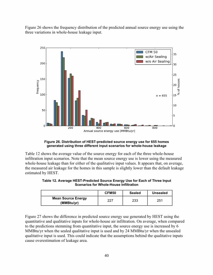
40

Figure 26 shows the frequency distribution of the predicted annual source energy use using the three variations in whole-house leakage input.

Figure 26. Distribution of HEST-predicted source energy use for 655 homes generated using three different input scenarios for whole-house leakage

Table 12 shows the average value of the source energy for each of the three whole-house infiltration input scenarios. Note that the mean source energy use is lower using the measured whole-house leakage than for either of the qualitative input values. It appears that, on average, the measured air leakage for the homes in this sample is slightly lower than the default leakage estimated by HEST.

Table 12. Average HEST-Predicted Source Energy Use for Each of Three Input Scenarios for Whole-House Infiltration

CFM50 Sealed Unsealed Mean Source Energy

(MMBtu/yr) 227 233 251

Figure 27 shows the difference in predicted source energy use generated by HEST using the quantitative and qualitative inputs for whole-house air infiltration. On average, when compared to the predictions stemming from quantitative input, the source energy use is increased by 6 MMBtu/yr when the sealed qualitative input is used and by 24 MMBtu/yr when the unsealed qualitative input is used. This could indicate that the assumptions behind the qualitative inputs cause overestimation of leakage area.

41

Figure 27. Distribution of differences in home energy score-predicted source energy use using qualitative and quantitative input for whole-house leakage

Additional analysis examining sensitivity in terms of the Home Energy Score to the quantitative and qualitative inputs for whole-house air infiltration is presented in Section 6.3.

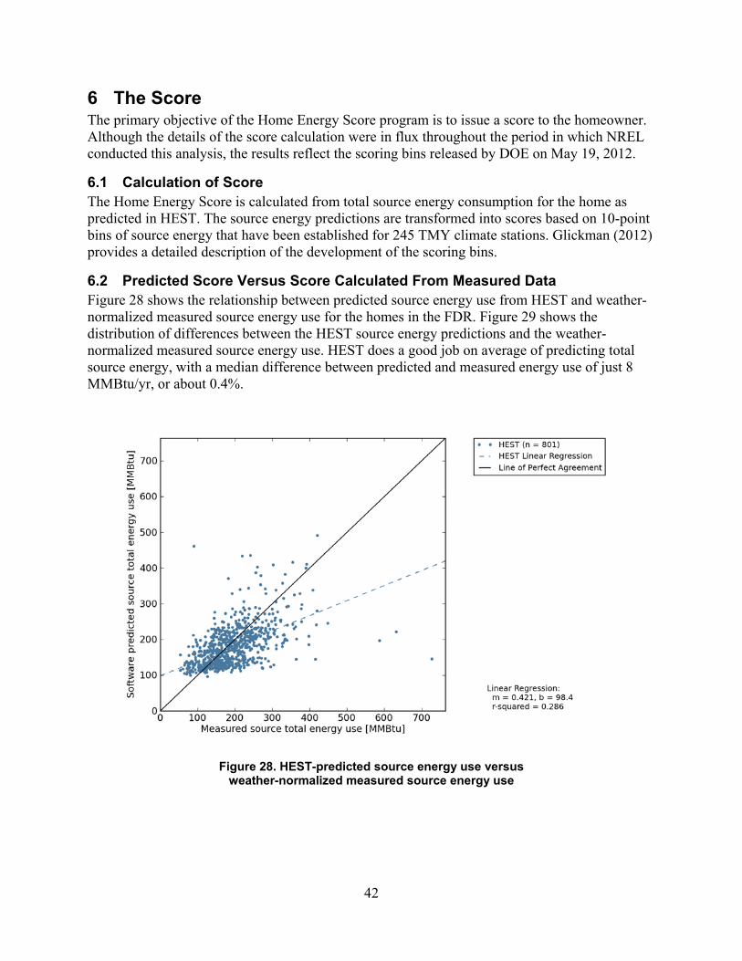
42

6 The Score The primary objective of the Home Energy Score program is to issue a score to the homeowner. Although the details of the score calculation were in flux throughout the period in which NREL conducted this analysis, the results reflect the scoring bins released by DOE on May 19, 2012.

6.1 Calculation of Score The Home Energy Score is calculated from total source energy consumption for the home as predicted in HEST. The source energy predictions are transformed into scores based on 10-point bins of source energy that have been established for 245 TMY climate stations. Glickman (2012) provides a detailed description of the development of the scoring bins.

6.2 Predicted Score Versus Score Calculated From Measured Data Figure 28 shows the relationship between predicted source energy use from HEST and weather-normalized measured source energy use for the homes in the FDR. Figure 29 shows the distribution of differences between the HEST source energy predictions and the weather-normalized measured source energy use. HEST does a good job on average of predicting total source energy, with a median difference between predicted and measured energy use of just 8 MMBtu/yr, or about 0.4%.

Figure 28. HEST-predicted source energy use versus weather-normalized measured source energy use

43

Figure 29. Distribution of differences between HEST-predicted and measured source energy use

Figure 30 shows the cumulative distribution of differences between HEST-predicted and measured source energy use. The median difference between predicted and measured source energy use is –8 MMBtu/yr; this can be observed at the 50% point on the x-axis in Figure 30. It can also be observed in Figure 30 that HEST underpredicts source energy use in about 60% of the homes.

44

Figure 30. Cumulative distribution of differences between HEST-predicted and measured source energy use26

Figure 31 is a bubble graph of the HEST-calculated score versus a score calculated from the weather-normalized measured source energy use for the homes in the FDR. The size of each bubble represents the number of occurrences at that point. The number of occurrences is also displayed numerically inside or alongside each bubble. The axes are inverted to make this figure comparable to those above; lower scores represent higher energy use.

26 Data points above 150% difference are not shown on the graph.

45

Figure 31. Predicted score versus score calculated from weather-normalized measured source energy use

Figure 32 shows a histogram of the differences between the HEST-calculated score and the score calculated from measured data. The mean and standard deviation of the differences are shown in the figure. For 52% of the homes in this sample, the predicted HEST is within ±1 point of a score calculated from measured energy use.

46

Figure 32. Histogram of differences between predicted score and score calculated from measured energy use

6.3 Sensitivity of Score to Assessment of Whole-House Leakage Figure 33 shows the frequency distribution of the score for 655 homes in the Home Energy Score Pilot using the three variations in whole-house leakage input:

• Using the blower door data

• Using the qualitative assessment of “sealed”

• Using the qualitative assessment of “unsealed.”

47

Figure 33. Distribution of Home Energy Score for 655 homes generated using three input values for whole-house leakage

Table 13 shows the average value of the Home Energy Score for each of the three whole-house infiltration modes. Note that the average score is higher using the measured whole-house leakage than for either of the qualitative input values. It appears that on average the measured air leakage for the homes in this sample is slightly lower than the default leakage estimated by HEST.

Table 13. Average Home Energy Score for Each of Three Input Scenarios for Whole-House Infiltration

CFM50 Sealed Unsealed

Mean Score: 5.75 5.59 5.08

Pearson’s chi-square test was applied to examine the relationship between the three distributions shown in Figure 33.27 The chi-square test tests whether the frequency distribution of observations in a sample is consistent with a historical or expected distribution. Treating the quantitative distribution as the expected distribution, and the two qualitative distributions as observed distributions, we were able to draw from chi-square tests the following statistical conclusions for this sample of homes:

• The sealed qualitative distribution is not significantly different from the quantitative distribution at a 95% CL.

27 Scoring bins 9 and 10 were pooled together because frequencies are less than 5 (an issue with chi-square tests).

48

• The unsealed qualitative distribution is significantly different from the quantitative distribution at > 99% CL. Hence, we can say with confidence that using the unsealed qualitative option reduces the mean score when compared to using the quantitative input method for the set of homes considered in this analysis.

Figure 34 shows the difference in Home Energy Score generated by HEST using the quantitative and qualitative inputs for whole-house air infiltration. On average, for this sample of homes, the Home Energy Score is reduced by 0.16 points when the sealed qualitative input is used and by 0.67 points when the unsealed qualitative input is used.

Figure 34. Distribution of differences in Home Energy Score generated using qualitative and quantitative input for whole-house leakage

An examination of the score sensitivity to the quantitative and qualitative inputs for whole-house air infiltration by climate28 was also conducted using the pilot data. No climate-specific issues were identified by the sensitivity study.

28 At the time of the pilot, the Home Energy Score was calculated using bins for 18 climate zones in the United States. The sensitivity study looked at variability in results across these zones.

49

7 References ASHRAE. (2002). ASHRAE Guideline 14-2002: Measurement of Energy and Demand Savings. Atlanta, GA: American Society of Heating, Refrigerating and Air-Conditioning Engineers.

Blasnik, M. (2011). E-mail communications.

Earth Advantage Institute, Conservation Services Group (EAI/CSG). (2009). Energy Performance Score (EPS) 2008 Pilot Findings & Recommendations Report. Energy Trust of Oregon.

Glickman, J. (2012). Home Energy Score: Findings from 2011 Pilot Program and Analysis. Washington, D.C. Buildings Technology Program, Office of Energy Efficiency and Renewable Energy, U.S. Department of Energy. (In draft.)

Hassel, S.; Blasnik, M.; Hannas, B. (2009). Houston Home Energy Efficiency Study. Raleigh, NC: Advanced Energy.

Hendron, R.; Engebrecht, C. (2010). Building America Research Benchmark Definition: Updated December 2009. Golden, CO: National Renewable Energy Laboratory. NREL/TP-550-47246.

Judkoff, R.; Polly, B.; Bianchi, M.; Neymark, J. (2010). Building Energy Simulation Test for Existing Homes (BESTEST-EX); Phase 1 Test Procedure: Building Thermal Fabric Cases. Golden, CO: National Renewable Energy Laboratory. NREL/TP-550-47427.

Nettleton, G.; Edwards, J. (2012). Data Collection-Data Characterization Summary, NorthernSTAR Building America Partnership, Building Technologies Program. Washington, D.C.: U.S. Department of Energy.

Pigg, S.; Nevius, M. (2000). Energy and Housing in Wisconsin: A Study of Single-Family Owner-Occupied Homes. Energy Center of Wisconsin, 199-1.

Polly, B. (2011). Improving the Accuracy of Software-Based Energy Analysis for Residential Buildings (Presentation). Golden, CO: National Renewable Energy Laboratory. NREL/PR-5500-52745.

Polly, B.; Kruis, N.; Roberts, D. (2011). Assessing and Improving the Accuracy of Energy Analysis for Residential Buildings. Golden, CO: National Renewable Energy Laboratory, NREL/TP-5500-50865; DOE/GO-102011-3243.

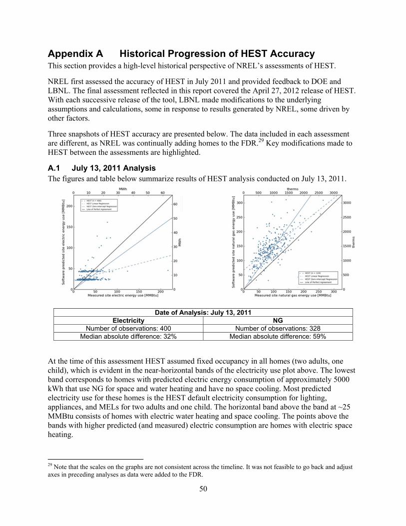
50

Appendix A Historical Progression of HEST Accuracy This section provides a high-level historical perspective of NREL’s assessments of HEST.

NREL first assessed the accuracy of HEST in July 2011 and provided feedback to DOE and LBNL. The final assessment reflected in this report covered the April 27, 2012 release of HEST. With each successive release of the tool, LBNL made modifications to the underlying assumptions and calculations, some in response to results generated by NREL, some driven by other factors.

Three snapshots of HEST accuracy are presented below. The data included in each assessment are different, as NREL was continually adding homes to the FDR.29 Key modifications made to HEST between the assessments are highlighted.

A.1 July 13, 2011 Analysis The figures and table below summarize results of HEST analysis conducted on July 13, 2011.

Date of Analysis: July 13, 2011 Electricity NG

Number of observations: 400 Number of observations: 328 Median absolute difference: 32% Median absolute difference: 59%

At the time of this assessment HEST assumed fixed occupancy in all homes (two adults, one child), which is evident in the near-horizontal bands of the electricity use plot above. The lowest band corresponds to homes with predicted electric energy consumption of approximately 5000 kWh that use NG for space and water heating and have no space cooling. Most predicted electricity use for these homes is the HEST default electricity consumption for lighting, appliances, and MELs for two adults and one child. The horizontal band above the band at ~25 MMBtu consists of homes with electric water heating and space cooling. The points above the bands with higher predicted (and measured) electric consumption are homes with electric space heating.

29 Note that the scales on the graphs are not consistent across the timeline. It was not feasible to go back and adjust axes in preceding analyses as data were added to the FDR.

51

HEST also significantly overpredicted NG consumption in this version of the tool.

A.2 July 20, 2011 Analysis Selected modifications to HEST in the July 20 update include:

• Neighboring houses on left and right assumed for shading calculations.

• Default thermostat now 78/84 cooling, 68/60 heating, compared to 78/81 and 68/64 previously.

• Default clothes washer loads now 1 warm/warm, 2 warm/cold, and 3 cold/cold per week.

• Increased DOE-2 wind shielding class, which will reduce local wind speeds.

• Conditioned basements now have thermostat setting 5 degrees lower than main living area for heating and 5 degrees higher for cooling, compared to no differential previously.

• Operable window shading now applied only during summer.

• Default refrigerator now a 10-year-old large, top freezer auto-defrost.

• Reduced default clothes dryer energy use, and number of loads to 5 per week.

• Reduced default dishwasher water use to 8.2 gallons/cycle and number of loads to 3 per week.

• Default water heater energy factors now 0.59 for gas and 0.90 for electric.

• Lowered default water heater set point to 120°F.

• Increased inlet water temperatures by approximately 8 degrees.

Date of Analysis: July 20, 2011 Electricity NG

Number of observations: 415 Number of observations: 334 Median absolute difference: 34% Median absolute difference: 25%

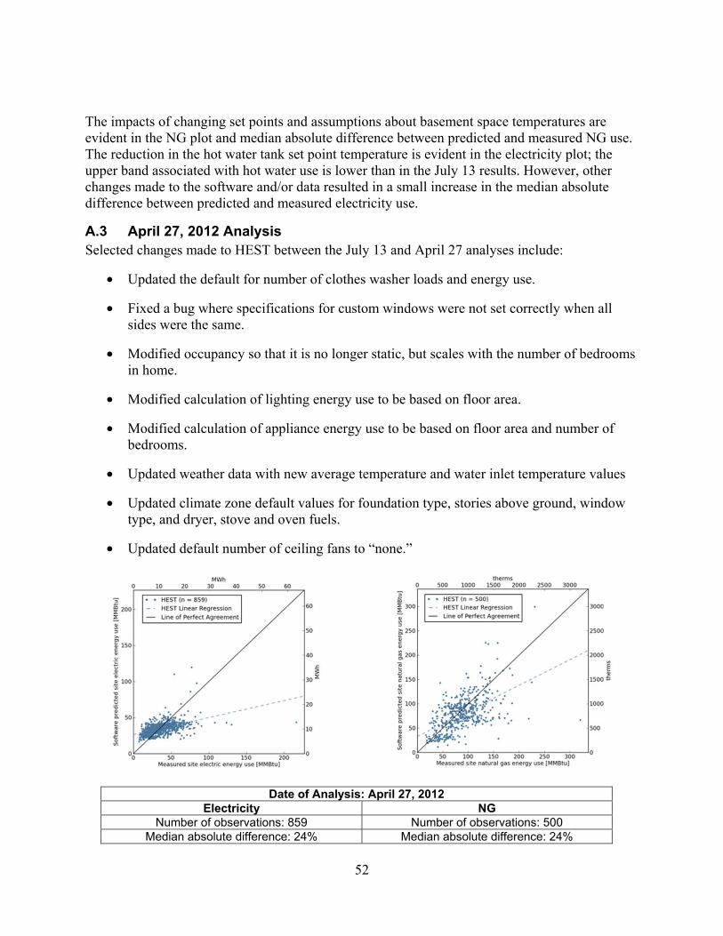
52

The impacts of changing set points and assumptions about basement space temperatures are evident in the NG plot and median absolute difference between predicted and measured NG use. The reduction in the hot water tank set point temperature is evident in the electricity plot; the upper band associated with hot water use is lower than in the July 13 results. However, other changes made to the software and/or data resulted in a small increase in the median absolute difference between predicted and measured electricity use.

A.3 April 27, 2012 Analysis Selected changes made to HEST between the July 13 and April 27 analyses include:

• Updated the default for number of clothes washer loads and energy use.

• Fixed a bug where specifications for custom windows were not set correctly when all sides were the same.

• Modified occupancy so that it is no longer static, but scales with the number of bedrooms in home.

• Modified calculation of lighting energy use to be based on floor area.

• Modified calculation of appliance energy use to be based on floor area and number of bedrooms.

• Updated weather data with new average temperature and water inlet temperature values

• Updated climate zone default values for foundation type, stories above ground, window type, and dryer, stove and oven fuels.

• Updated default number of ceiling fans to “none.”

Date of Analysis: April 27, 2012 Electricity NG

Number of observations: 859 Number of observations: 500 Median absolute difference: 24% Median absolute difference: 24%

53

Changes made in standard occupancy assumptions had a considerable impact on the predicted electricity use, reducing the median absolute difference between predicted and measured energy use from 34% in the July 20 analysis to 24% in the April 27 analysis. The horizontal bands evident in the July 13 and July 20 electricity plots are no longer seen in the plot above; the predicted electricity use trends upward with increasing measured electric energy use.

54

Appendix B Use of Field Data Repository in Scoring Tool Assessment

This section describes the state and use of the FDR in the HEST assessment project.

B.1 Field Data Repository Data Collection NREL has been working to obtain historical datasets containing robust, research-grade characteristics data coupled with utility billing data. It has proven to be a challenging process; there are many obstacles, including paucity of data and legal issues related to customer privacy. Nevertheless, NREL managed to accumulate useful data.

To start with, the FDR team focused on datasets that were available in the form of REM/Rate software input files. REM/Rate has been the most widely used home energy rating software for more than a decade, and thus REM/Rate input files are a relatively common format for existing datasets. It is used for home energy ratings (primarily supporting ENERGY STAR Qualified Homes Program), state and utility efficiency programs, and income-qualified weatherization programs. The software is used to evaluate new construction and retrofits, and its input files contain fairly detailed building characteristics. The software also has a feature that allows batch exporting of input files into a relational database. This REM/Rate database format became the starting point for the FDR.

Initial datasets that were collected and aggregated into the FDR included:

• Oregon Energy Performance Pilot Study (Earth Advantage Institute, Conservation Services Group 2009) data. A mix of 190 newer and older homes audited in 2008 and located in Portland and Bend.

• Wisconsin Housing Characterization Study (Pigg and Nevius 2000) data. Collected in 1991, a mix of 299 new and existing homes located throughout Wisconsin.

• Houston utility study. A sub-sample of 82 homes statistically derived from a utility program evaluation conducted by Hassel et al. in 2008 involving a sample of 226,000 homes built from 2002 through 2007.

• Advance Energy’s SystemVision homes. Four hundred ninety high-efficiency homes receiving full home energy ratings in North Carolina and Tennessee.

• Building America Energy Audit Assessment Housing Characterization (Nettleton and Edwards 2012) data. One hundred twenty-five older retrofit-candidate homes receiving full home energy ratings in Minnesota and Wisconsin.

• EPA ENERGY STAR Qualified Homes evaluation study. Seventy-five ENERGY STAR Qualified Homes in Minnesota and Wisconsin.

These datasets resulted in a total of 1183 homes in the FDR after processing them as described in the next section.

55

B.2 Field Data Repository Data Processing Housing characteristics data across these initial datasets were consistent and required no processing. The data were aggregated using REM/Rate batch database capabilities.

Utility billing data had to be processed for a subset of the datasets. To compare predicted energy use from HEST, SIMPLE, and REM/Rate to measured energy use, the utility billing data needed to be normalized for differences between the weather occurring during the utility billing period and the climate data used in the energy simulation. HEST, SIMPLE and REM/Rate use TMY2 climate data—TMY data for the 30-year period 1961–1990.

The utility billing data were weather normalized following the procedures outlined in ASHRAE Guideline 14-2002, Annex D: Regression Techniques (ASHRAE 2002). The requirement for 12 months of monthly billing data was waived and lowered to 10 months of billing data to increase the number of homes included in the resulting dataset. Three-parameter heating and cooling variable-base degree-day models were used, regressing monthly utility billing data against monthly degree-days calculated from coincident daily average temperatures. Historic daily average temperatures were obtained from weather stations managed by the National Climatic Data Center (NCDC)30.

Heating models were created with NG billing data and both heating and cooling models were created with electricity billing data. For each model, goodness-of-fit criteria were established as adjusted R2 ≥ 0.7 for gas and adjusted R2 ≥ 0.5 for electricity. For cases with insufficient goodness-of-fit, the model coefficients were not used and an annual average energy use was calculated from the utility billing data. For cases with fewer than 12 months of billing data, a daily average energy use was calculated and multiplied by 365.25 to calculate an annual energy use. For cases with more than 12 months of data, the annual energy use was calculated by summing the average energy use for each calendar month. For regression models with sufficient goodness-of-fit, the model coefficients were applied to the calculated degree-days from TMY2 climate data, calculating the normalized annual consumption. Daily HDDs and CDDs for TMY2 climate data were calculated at base temperatures ranging from 40°F to 70°F. Daily average temperatures were calculated from hourly TMY2 data before use in the calculation of daily degree-days.

Utility billing data could not be obtained for the Oregon dataset, but climate-normalized annual energy uses for electricity and NG were provided by Earth Advantage Institute.

B.3 Translation of Field Data Repository Data to Software Inputs For this project, “interpreters” were written in the Python programming language to translate FDR data to software inputs for HEST and SIMPLE. Detailed descriptions of these data translations are presented Appendix C and Appendix D.

B.4 Processing FDR Results Results for NG and electricity use were converted to MMBtu for analysis. HEST source energy was calculated using national average site-to-source multipliers. Only homes for which successful results were returns from all three software packages and sufficient utility bills could be obtained were included in the analysis.

30 Web url: http://www.ncdc.noaa.gov/oa/climate/stationlocator.html

56

Appendix C Translation of Field Data Repository Data to HEST Inputs

In translating inputs from the FDR to HEST, the goal was to provide an “out-of-the-box” set of inputs to HEST. In other words, to use HEST as close to how an assessor entering data would use it. The following is an explanation of each input to HEST and how it was derived from FDR data. The HEST input variables are identified by italicsAndCamelCase.

C.1 General • Zipcode—The ZIP code from the house address in REM/Rate was used. For homes

without a ZIP code recorded, the zip code was looked up for the city and state using postal code data from the Geonames Project.31

• year—The year the house was built.

C.2 House Shape and Size • houseOrientation—In the FDR data the orientation of the windows is known. Overall

house orientation is not known. House orientation was estimated by taking the side of the house with the greatest window area and assuming that it is the back of the house.

• storiesAboveGround— Number of above ground stories was retrieved from the FDR.

• floorArea—Total conditioned floor area was retrieved from the FDR.

• ceilingHeight—Average ceiling height was calculated by dividing the total conditioned volume by the floor area. The result was rounded to the nearest foot.

C.3 Number of Bedrooms • numberBedrooms— Number of bedrooms was retrieved from the FDR.

C.4 Airtightness • airLeakage50ip—The blower door measurement, measured in CFM50. If the infiltration

was measured in air changes per hour at 50 Pascals (ACH50) it was converted to CFM50 using 50 = 50 ∙ 60⁄ If the infiltration was measured in CFM25, it was converted to CFM50 using 50 = 25 ∙ (50 25⁄ ) .

• airSealingPresent—If the infiltration units were not measured in CFM50, CFM25, or ACH50, the infiltration measurement was omitted in HEST and the house was marked as “not air sealed,” the HEST default.

31 http://www.geonames.org

57

C.5 Foundation and Floor • foundationType—The following mapping was used to convert foundation type from FDR

to HEST compatible foundation types:

FDR Foundation Type HEST Foundation Type Slab Slab-on-grade foundation

Open Crawlspace Vented crawlspace Enclosed Crawlspace ‘Unvented Crawlspace’ if the crawlspace type

in REM/Rate is ‘Unvented’. ‘Vented Crawlspace’ if the crawlspace type in

REM/Rate is ‘Vented’ or ‘Operable Vents’. Conditioned Basement Conditioned Basement

Unconditioned Basement Unconditioned Basement Conditioned Crawlspace Unvented Crawlspace

If the foundation type was “more than one foundation type” the foundation wall or slab with the greatest perimeter to ambient/ground was specified as the foundation type in HEST.

• foundationSideInsulationRValue—If the foundation type was a slab the R-value of the slab insulation with the greatest area was returned and rounded to the nearest of R-0 or R-5 (the only options for slab insulation in HEST). If the foundation type was a basement or crawlspace, the sum of the exterior, cavity, and interior rigid insulation R-values of the foundation wall with the greatest area was returned and rounded to the nearest of R-0, 11, and 19 (the only options for basement and crawlspace foundation insulation in HEST).

• floorConstruction—Insulation level of the floor above the basement or crawlspace. This was calculated by identifying the largest frame floor between conditioned space and the open crawlspace, enclosed crawlspace, conditioned basement, or unconditioned basement depending on the foundation type, and then adding the cavity and continuous insulation R-values and rounding to the closest of R-0, 11, 13, 15, 19, 21, 25, 30, and 38 (the only available options in HEST). Other foundation types were assumed to have zero floor insulation.

C.6 Walls • wallsSameAllSides—Indicates if different wall types are described on each side of the

house or if one wall type is used to describe all of the exterior walls. This input was always set to true to specify one wall type for the whole house.

• wallConstructionFront—Represents the construction of all of the walls in this case because the wallsSameAllSides input above was set to true. Wood stud walls were input with the cavity insulation rounded to the closest of the available R-values in HEST (0,3,7,11,13,15,19,21). Any continuous insulation on a wood stud wall was assumed to be 1-in. extruded polystyrene sheathing, as that was the only available option in the HEST interface. All siding on wood stud walls was assumed to be wood. Structural brick walls and concrete block walls, where applicable, were also translated accordingly. The R-

58

values of the continuous insulation were rounded to the nearest values available in the HEST input (R-0, 5, 10 and R-0, 3, 6, respectively).

C.7 Doors and Windows • windowArea(Front|Back|Left|Right)—Window area was totaled for each side and

returned. For windows facing a direction between two sides (e.g., facing northeast), the window area was divided between the two sides (half area facing north, half area facing east).

• windowUValue(Front|Back|Left|Right)—An area-weighted average U-value was calculated for each window direction.

• windowSolarGain(Front|Back|Left|Right)—An area-weighted average SHGC was calculated for each window direction.

• windowShade(Front|Back|Left|Right—An area-weighted average interior shading factor was calculated for each window direction. A qualitative input was then selected that most closely matched the values in Table 9, p. 89, of the HEST documentation.32

C.8 Skylights • skylightsPresent—For homes with any skylight area, this was set to “true”. For homes

with no skylight area, this was set to “false” and no other skylight inputs were specified.

• skylightType—A skylight from the HEST library was selected that most closely matched the area-weighted average U-value and SHGC of the skylights on the house.

• skylightArea—Total skylight area.

C.9 Attic and Roof Only one ceiling can be specified in HEST. The ceiling with the greatest area for the house in the FDR was selected. All others were ignored.

• atticType—‘Vaulted’ ceiling in FDR was translated to a ‘Cathedral Ceiling’ in HEST. ‘Attic’ in FDR was translated to ‘Unconditioned Attic’ in HEST.

• roofConstruction—This input is a code that represents the roofing material, roof insulation (not attic floor insulation), and the presence of a radiant barrier. All roofs were assumed to have composition shingles. For roofs with vaulted ceilings, the insulation indicated in the FDR was assumed to be in the roof cavity and the nearest R-value (R-0, 11, 13, 15) available for roof insulation in HEST was selected. If a roof had a radiant barrier and no roof insulation then a radiant barrier was selected in HEST. For roofs above an unfinished attic, no insulation was specified in the roofContruction, but was instead specified on the attic floor in ceilingConstruction.

• ceilingConstruction—This indicates the R-value of insulation on the attic floor. For roofs above an unfinished attic, the R-value from the FDR was assumed to be on the attic floor and the nearest option for attic floor insulation in HEST was selected (R-0, 3, 9, 11, 19, 21, 25, 30, 38, 49, 60). For roofs above a vaulted ceiling, no insulation was specified in the ceilingConstruction.

32 http://evanmills.lbl.gov/pubs/pdf/home-energy-saver.pdf

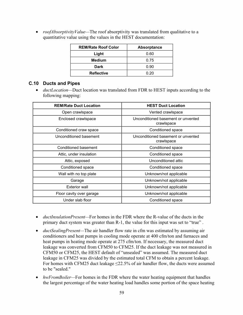
59

• roofAbsorptivityValue—The roof absorptivity was translated from qualitative to a quantitative value using the values in the HEST documentation:

REM/Rate Roof Color Absorptance

Light 0.60

Medium 0.75

Dark 0.90

Reflective 0.20

C.10 Ducts and Pipes • ductLocation—Duct location was translated from FDR to HEST inputs according to the

following mapping:

REM/Rate Duct Location HEST Duct Location

Open crawlspace Vented crawlspace

Enclosed crawlspace Unconditioned basement or unvented crawlspace

Conditioned craw space Conditioned space

Unconditioned basement Unconditioned basement or unvented crawlspace

Conditioned basement Conditioned space

Attic, under insulation Conditioned space

Attic, exposed Unconditioned attic

Conditioned space Conditioned space

Wall with no top plate Unknown/not applicable

Garage Unknown/not applicable

Exterior wall Unknown/not applicable

Floor cavity over garage Unknown/not applicable

Under slab floor Conditioned space

• ductInsulationPresent—For homes in the FDR where the R-value of the ducts in the primary duct system was greater than R-1, the value for this input was set to “true” .

• ductSealingPresent—The air handler flow rate in cfm was estimated by assuming air conditioners and heat pumps in cooling mode operate at 400 cfm/ton and furnaces and heat pumps in heating mode operate at 275 cfm/ton. If necessary, the measured duct leakage was converted from CFM50 to CFM25. If the duct leakage was not measured in CFM50 or CFM25, the HEST default of “unsealed” was assumed. The measured duct leakage in CFM25 was divided by the estimated total CFM to obtain a percent leakage. For homes with CFM25 duct leakage ≤22.5% of air handler flow, the ducts were assumed to be "sealed."

• hwFromBoiler—For homes in the FDR where the water heating equipment that handles the largest percentage of the water heating load handles some portion of the space heating

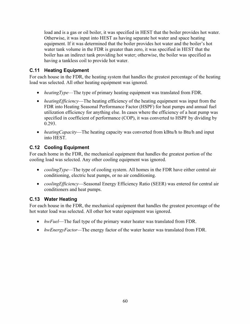
60

load and is a gas or oil boiler, it was specified in HEST that the boiler provides hot water. Otherwise, it was input into HEST as having separate hot water and space heating equipment. If it was determined that the boiler provides hot water and the boiler’s hot water tank volume in the FDR is greater than zero, it was specified in HEST that the boiler has an indirect tank providing hot water; otherwise, the boiler was specified as having a tankless coil to provide hot water.

C.11 Heating Equipment For each house in the FDR, the heating system that handles the greatest percentage of the heating load was selected. All other heating equipment was ignored.

• heatingType—The type of primary heating equipment was translated from FDR.

• heatingEfficiency—The heating efficiency of the heating equipment was input from the FDR into Heating Seasonal Performance Factor (HSPF) for heat pumps and annual fuel utilization efficiency for anything else. In cases where the efficiency of a heat pump was specified in coefficient of performance (COP), it was converted to HSPF by dividing by 0.293.

• heatingCapacity—The heating capacity was converted from kBtu/h to Btu/h and input into HEST.

C.12 Cooling Equipment For each home in the FDR, the mechanical equipment that handles the greatest portion of the cooling load was selected. Any other cooling equipment was ignored.

• coolingType—The type of cooling system. All homes in the FDR have either central air conditioning, electric heat pumps, or no air conditioning.

• coolingEfficiency—Seasonal Energy Efficiency Ratio (SEER) was entered for central air conditioners and heat pumps.

C.13 Water Heating For each house in the FDR, the mechanical equipment that handles the greatest percentage of the hot water load was selected. All other hot water equipment was ignored.

• hwFuel—The fuel type of the primary water heater was translated from FDR.

• hwEnergyFactor—The energy factor of the water heater was translated from FDR.

61

Appendix D Translation of Field Data Repository Data to SIMPLE Inputs

In translating inputs from the FDR to SIMPLE, the goal was to provide an “out-of-the-box” set of inputs to SIMPLE. In other words, to use SIMPLE as close to how it would be used by an auditor entering data. However, in many cases the data collected were in a different form and needed to be translated. Specifically, in SIMPLE most of the inputs are qualitative in nature with numeric overrides in an override section of the spreadsheet. The FDR data are primarily numeric. To avoid introducing additional error by converting the numeric values in FDR to approximate qualitative values for input to SIMPLE, the numeric overrides were used whenever possible.

Following is an explanation of each input to SIMPLE and how it was derived from REM/Rate data.

D.1 General House Characteristics • Closest Weather Station—The closest weather station was selected from the ZIP code of

the house address in REM/Rate. For homes without a ZIP code recorded, the ZIP code was looked up for the city and state using postal code data from the Geonames Project.33

• Finished floor area (above grd)—For homes in the FDR with a conditioned basement, the total conditioned floor area was divided by the number of stories plus one (for the basement) to estimate the average conditioned floor area per floor. The floor area per floor was then multiplied by the number of above ground stories to estimate the finished floor area above ground.

• Stories—Number of above ground stories was retrieved from the FDR.

• Bedrooms—Number of bedrooms was retrieved from the FDR.

D.2 Heating System • Primary Heating Fuel—This input describes the fuel used for the primary heating

equipment. However, for electric heating it requires a selection of whether it is resistance heating, a heat pump, or a heat pump with a gas backup. For each home in the FDR, the heating system that handles the largest portion of the space-heating load was selected. The primary heating fuel was retrieved from that equipment and for electric heating equipment the appropriate equipment type was selected.

• Heating System Type—The heating system type is a qualitative description of the heating system efficiency. This input was overridden by the quantitative Heating Efficiency input.

• Heating Efficiency (override)—Heating efficiency was calculated for the primary heating system in the metric appropriate for the fuel type (COP for electric, annual fuel utilization efficiency for gas). For electric resistance heating, the efficiency was allowed to default in SIMPLE. Since the numeric efficiency of electric heating did not change when different qualitative efficiency inputs were selected the efficiency was assumed to be part of the logic of the SIMPLE and not intended to be an input in this case. The efficiency of air source heat pumps and dual-fuel heat pumps was converted from HSPF to COP. Then,

33 http://www.geonames.org

62

a climate adjustment was applied to the COP of air source heat pumps (not dual-fuel heat pumps) according to a method recommended by Blasnik & Associates.

• Heat Distribution Type—The heating distribution type was selected based on the type of heating equipment (ducts for furnaces, radiators for boilers, etc.).

• Secondary Heating Type—This input allows the same selections as the Primary Heating Fuel input described above with the addition of hard and soft woods. For each home in the FDR with more than one heating system, the one that handles the second-largest portion of the space heating load was selected and translated in the same manner as the Primary Heating Fuel input. If the secondary heating system burns wood, ‘Soft’ wood was assumed and submitted to SIMPLE.

• Secondary heating - % home—The percentage of the heating load handled by the secondary heating system as retrieved from the FDR. If there are more than two heating systems, the primary heating system assumed the load of the third, fourth, etc. systems. For homes in the FDR with only one heating system this input was set to zero.

D.3 Walls • Wall Insulation—A qualitative description of the wall insulation (e.g., “No Ins”,

“Partial”, “Std.”, “Good”, “Very Good”). This input was overridden by the quantitative Wall R override.

• Wall Area (override)—Overrides the default calculated wall area within SIMPLE. The wall with the largest area between conditioned and ambient space was selected for each house in the FDR and the area of that wall was submitted.

• Wall Area 2 (override)—For homes in the FDR with more than one wall type between conditioned and ambient spaces, the second largest area was selected and submitted. Additional wall area between conditioned and ambient space was added to the first wall (Wall Area above).

• Wall R (override)—The assembly R-value is selected from the primary wall type for each house as determined in the Wall Area input above. If the wall assembly R-value from the FDR was less than R-6, the R-value was set to R-6 to replicate the “no insulation” condition in the Wall Insulation qualitative input.

• Wall 2 R (override)—The assembly R-value of the secondary wall type was calculated similarly to the Wall R input.

D.4 Attics • Attic Insulation—A qualitative description of the attic insulation (e.g. “None”, “Some”,

“Std. 10 inch”, “High Ins”). This input was overridden by the quantitative Attic R override.

• Attic Area (override)—Overrides the default calculated attic area within SIMPLE. For each house in the FDR, the attic with the greatest area was selected as the primary attic and the area of that attic was submitted.

63

• Attic Area 2 (override)—For homes in the FDR with more than one attic type, the second largest attic area was selected and submitted. Additional attic area was attributed to the first attic (Attic Area above).

• Attic R (override)—The total R-value of the primary attic (as determined for the Attic Area input above) was selected from the FDR. If the attic had a calculated R-value less that R-5, the R-value was set to R-5 to replicate the “no insulation” condition in the qualitative input (Attic Insulation).

• Attic 2 R (override)—The assembly R-value of the secondary attic was calculated similarly to the Attic R input.

D.5 Windows • Window Type—A qualitative description of the type of windows installed on the house

(e.g. “Single”, “Dbl/Sng&Storm”, “Dbl & low e”, “Super”). This is overridden by the Windows R override as described below.

• Window Area—A qualitative description of the relative amount of window area (e.g. “High”, “Typical”, “Low”). This is overridden by the Windows Area override as described below.

• Windows Area (override)—Square feet of window area. For each home in the FDR the window area is summed and submitted.

• Windows R (override)—An area-weighted average window R-value was calculated from the FDR data and submitted.

D.6 Infiltration • Air Tightness—A qualitative description of the air tightness of the house (e.g. “Very

Leaky”, “Leaky”, “Average”, “Fairly Tight”, “Tight”, “HRV”). This is overridden by the CFM50 Air Leakage override as described below.

• CFM50 Air Leakage (override)—The qualitative airtightness input was overridden by the blower door measurement measured in CFM50. If the infiltration was measured in ACH50 it was converted to CFM50 using 50 = 50 ∙ 60⁄ If the infiltration was measured in CFM25, it was converted to CFM50 using 50 = 25 ∙ (50 25⁄ ) .

D.7 Foundation • Foundation Type—Foundation types from FDR were translated to SIMPLE according to

the following mapping:

64

REM/Rate Foundation Type SIMPLE Foundation Type

Slab Slab

Open crawlspace Crawlspace

Enclosed craw space Crawlspace

Conditioned basement Basement conditioned

Unconditioned basement Basement

More than one type Varies, see below

Apartment above conditioned space Throws an error

Conditioned crawlspace Crawlspace conditioned

Where there was more than one foundation type, the foundation type was determined from the foundation wall or slab with the greatest perimeter adjacent to outdoors.

• Foundation Insulation—A qualitative input describing the location of the foundation insulation (e.g. “None”, “Walls”, “Ceiling”). If the foundation type was a slab, “None” was assumed for foundation insulation. Otherwise, the R-values of the largest frame floor area recorded and the largest foundation wall area were compared and the one with the larger R-value was assumed to be insulated.

D.8 Ducts • Ducts: % in Attic—The percentage of the supply ducts in the attic from the FDR were

summed and entered into SIMPLE.

• Ducts: % in Basement—The percentage of supply ducts in the basement was similarly calculated.

• Duct Insulation—Area weighted average duct insulation R-value was calculated and then the duct insulation level available in SIMPLE closest to that R-value was selected.

• Duct Leakiness—Duct leakage in CFM25 was calculated for each duct and averaged by floor area served. Duct leakage measured in CFM50 was converted to CFM25 using 25 = 50 ∙ (25 50⁄ ) .

Total air handler CFM was estimated at 400 CFM/ton for an air conditioners and heat pumps in cooling mode or 275 CFM/ton for furnaces and heat pumps in heating mode. Blasnik & Associates indicated (Blasnik 2011) that the qualitative inputs for duct leakage corresponded to the following CFM25 values for a 1200 CFM air handler:

65

Duct Leakage Description CFM25 Leakage for a 1200 CFM Air Handler

Very Leaky 700

Leaky 500

Average 300

Tight 100

Airtight 0

Those values were then scaled to the approximated size of air handler. The qualitative duct leakage with the scaled value closest to the averaged CFM25 was entered into SIMPLE.

D.9 Cooling For homes in the FDR with multiple central air, air-source heat pump, or dual-fuel heat pump systems, the equipment that handles the greatest percentage of the cooling load was assumed to be the only cooling system.

• AC SEER—For each home in the FDR, the efficiency of the primary air conditioning system, measured in SEER, was submitted to SIMPLE. If the efficiency was recorded in EER it was converted to SEER using the following equation from the Building America House Simulation Protocols (Hendron and Engebrecht 2010):

EER = -0.02 × SEER2 + 1.12 × SEER

• Window Shading—Shading was calculated based on data from the FDR by taking the average of the summer and winter internal shading coefficients multiplied by the average of the summer and winter external shading coefficients for each window. Then, the overall shading coefficient was calculated as the area-weighted average of the shading coefficients of each window. A shading choice was then selected from the list in SIMPLE based on which choice corresponded most closely to the calculated shading coefficient.

• Cool Roof / Rad. Barrier rafters—A quantitative input describing the absorptivity of the roof (e.g. “Std Color”, “Reflective / low gain”, “Very Reflective”). For each home in the FDR, the absorptivity of the largest roof was used to select the option that corresponded most closely in SIMPLE. If the roof was marked as having a radiant barrier in the FDR, the input was then changed to ‘Very Reflective’, as per guidance from Blasnik & Associates (Blasnik 2011).

D.10 Water Heating • Water Heater Fuel—For each house in the FDR, the water heating system that covers the

largest percentage of the hot water load was used to determine the fuel type for input into SIMPLE.

• Water Heater Type—For each house in the FDR, the water heating system that covers the largest percentage of the hot water load was used to determine the type of water heater installed (e.g. “Standard”, “Tankless”, “High Efficiency”, “Indirect”, “Integrated”, “Heat Pump”). For conventional tank water heaters, the water heater was assumed to be ‘High

66

Efficiency’ if the energy factor was greater than 0.9 and the fuel was not electricity (Blasnik 2011). Otherwise, the water heater was assumed to be ‘Standard.’ Other translations of the FDR water heater types were fairly straightforward (e.g., ‘Instant’ translates to ‘Tankless’).

• Hot Water Fixture Efficiency—Assumed to be Average.

D.11 All Else Information34 • Lighting Efficiency—Assumed to be “Average”.

• Primary Refrigerator—For homes in the FDR where a default refrigerator was specified, an ‘Average’ refrigerator was selected in SIMPLE.

• Refrigeration (override)—Specifies kilowatt-hours per year of refrigerator energy use and overrides the Primary Refrigerator input above. For homes in the FDR where a user-defined refrigerator was specified, the refrigerator data were available in terms of total kWh/yr of refrigerator energy use (adding the energy use of more than one refrigerator, if necessary). Those data were then used here to override the Primary Refrigerator input.

• Extra Refrigerators / Freezers—Assumed to be “None”.

• Entertainment (TVs & PCs)—Assumed to be “Average”.

• # Other Large Uses (500 kWh)—Number of other electricity uses near 500 kWh/yr. Assumed to be zero.

• Other Plug Loads—Assumed to be “Average”.

• Clothes Dryer Fuel—Retrieved from the FDR for each house.

• Cooking Fuel—Retrieved from the FDR for each house.

D.12 Occupancy and Behavior • Occupants—Set to zero, which caused SIMPLE to make a default assumption about

occupancy based on other inputs.

• Heating Setpoint—The average heating setpoint was selected to match the average of the heating set point schedule35 in HEST: 65°F.

• Cooling Setpoint—The average cooling setpoint was selected to match the average of the cooling set point schedule36 in HEST: 80.25°Ft.

34 All Else Information is SIMPLE terminology. 35 http://goo.gl/SaRof 36 http://goo.gl/SaRof

67

Appendix E Additional Statistical Model Information Included in this appendix are additional information and background materials for the statistical models developed in Section 3. Additional validations of the difference models are provided. A complete list of coded variables and descriptions are included.

E.1 Additional Validation of MLR models In Section 3, measured energy use and differences (predicted minus measured) in energy use were modeled separately for each energy type. Because the models of differences had very low R-squared values, an additional validation was done. By adding the MLR prediction for differences to the MLR prediction for measured, an MLR prediction of the HEST prediction is obtained. Hence, a simple linear regression can be applied for HEST prediction as a function of this combined MLR prediction.

The figure below shows the HEST prediction versus the MLR prediction for site electricity use. The data shown are from the test set. The adjusted R-squared was 0.723, which can be interpreted that the MLR models can recover approximately 72% of the HEST prediction.

HEST prediction versus combined MLR models for measured site electricity

0 10 20 30 40 50 60

02

04

06

08

0

Test Set

MLR Combined Site Electricity (MMBtu)

Pre

dic

ted

Site

Ele

ctri

city

(MM

Btu

)

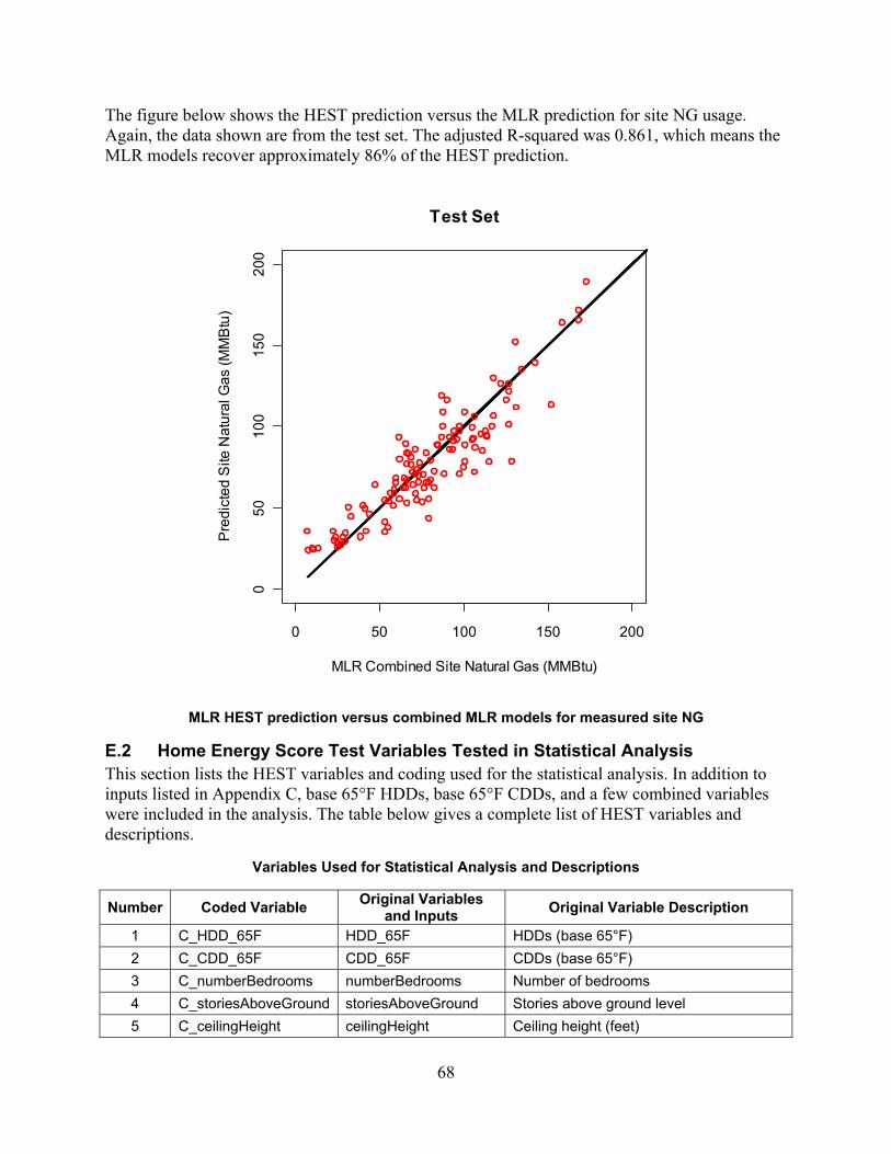
68

The figure below shows the HEST prediction versus the MLR prediction for site NG usage. Again, the data shown are from the test set. The adjusted R-squared was 0.861, which means the MLR models recover approximately 86% of the HEST prediction.

MLR HEST prediction versus combined MLR models for measured site NG

E.2 Home Energy Score Test Variables Tested in Statistical Analysis This section lists the HEST variables and coding used for the statistical analysis. In addition to inputs listed in Appendix C, base 65°F HDDs, base 65°F CDDs, and a few combined variables were included in the analysis. The table below gives a complete list of HEST variables and descriptions.

Variables Used for Statistical Analysis and Descriptions

Number Coded Variable Original Variables

and Inputs Original Variable Description

1 C_HDD_65F HDD_65F HDDs (base 65°F)

2 C_CDD_65F CDD_65F CDDs (base 65°F)

3 C_numberBedrooms numberBedrooms Number of bedrooms

4 C_storiesAboveGround storiesAboveGround Stories above ground level

5 C_ceilingHeight ceilingHeight Ceiling height (feet)

0 50 100 150 200

05

01

00

15

02

00

Test Set

MLR Combined Site Natural Gas (MMBtu)

Pre

dic

ted

Site

Nat

ura

l Gas

(M

MB

tu)

69

Number Coded Variable Original Variables

and Inputs Original Variable Description

6 C_floorArea floorArea Floor area (ft2)

7 C_houseOrientation houseOrientation House orientation degrees (north = 0, east = 90, south = 180, and west = 270)

8 C_airLeakage50ip airLeakage50ip Air Leakage (cubic feet per minute)

9 C_roofAbsorptance roofAbsorptance Roof absorptance

10 C_fndtnInsulRValue foundation-SideInsulationRValue

Foundation side insulation R-value

11 C_skylightArea skylightArea Skylight area (ft2)

12 C_windowAreaTotal windowArea Window area total

13 C_WAU_Total windowArea*U sum((Window area) × (U-factors))

14 C_WASG_Total windowArea*SHGC sum((Window area) × (SHGC))

15 C_N_windowArea

windowAreaFront, windowAreaRight, windowAreaBack, and windowAreaLeft

Direction of window area determined from houseOrientation

16 C_E_windowArea same as above same as above

17 C_S_windowArea same as above same as above

18 C_W_windowArea same as above same as above

19 C_N_WAU Directional windowArea*U (Window area) × (U-factors)

20 C_E_WAU same as above same as above

21 C_S_WAU sames as above same as above

22 C_W_WAU same as above sames as above

23 C_N_WASG Directional windowArea*SHGC (Window area) × (SHGC)

24 C_E_WASG sames as above same as above

25 C_S_WASG same as above same as above

26 C_W_WASG same as above same as above

27 C_heatingEfficiency heatingEfficiency System heating efficiency

28 C_coolingEfficiency coolingEfficiency Cooling efficiency for air conditioner

29 C_hwFuel hwFuel Hot water fuel type (gas or electric)

30 C_hwEnergyFactor hwEnergyFactor Hot water energy factor

31 C_RoofRValue roofRValue Roof R-value determined from roof construction and ceiling construction inputs

32 C_FloorRValue floorRValue Floor R-value determined from floor construction input

33 C_WallRValue wallRValue Wall R-value determined from wall construction input

34 Bend_OR Bend, OR Bend, Oregon in climate zone 18

35 Built_2001_plus from yearBuilt House built in 2001 or later

36 Built_1976_to_2000 House built between 1976 and 2000

70

Number Coded Variable Original Variables

and Inputs Original Variable Description

37 Built_1951_to_1975 House built between 1951 and 1975

38 C_HT_GBL heatingType Heating type GBL (gas boiler)

39 C_HT_GWF Heating type GWF (gas wall furnace)

40 C_HT_EBB Heating type EBB (electric baseboard)

41 C_HT_EFN Heating type EFN (electric furnace)

42 C_HT_EHP Heating type EHP (electric heat pump)

43 C_RC_rfps11co roofConstruction Roof construction code rfps11co

44 C_RC_rfps15co Roof construction code rfps15co

45 C_RC_rfrb00co Roof construction code rfrb00co

46 C_RC_rfwf00co Roof construction code rfwf00co

47 C_RC_rfwf11co Roof construction code rfwf11co

48 C_RC_rfwf15co Roof construction code rfwf15co

49 C_AT_cath_ceil atticType Attic type of cathedral ceiling

50 C_CC_ecwf00 ceilingConstruction Ceiling construction code ecwf00

51 C_CC_ecwf03 Ceiling construction code ecwf03

52 C_CC_ecwf06 Ceiling construction code ecwf06

53 C_CC_ecwf09 Ceiling construction code ecwf09

54 C_CC_ecwf19 Ceiling construction code ecwf19

55 C_CC_ecwf21 Ceiling construction code ecwf21

56 C_CC_ecwf25 Ceiling construction code ecwf25

57 C_CC_ecwf30 Ceiling construction code ecwf30

58 C_CC_ecwf38 Ceiling construction code ecwf38

59 C_FT_slab foundationType Foundation type code slab

60 C_FT_uncond_base Foundation type code uncond_base

61 C_FT_unvent_crawl Foundation type code unvent_crawl

62 C_FT_vent_crawl Foundation type code vent_crawl

63 C_FC_efwf00ca floorConstruction Floor construction code efwf00ca

64 C_FC_efwf11ca Floor construction code efwf11ca

65 C_FC_efwf13ca Floor construction code efwf13ca

66 C_FC_efwf15ca Floor construction code efwf15ca

67 C_FC_efwf19ca Floor construction code efwf19ca

68 C_FC_efwf21ca Floor construction code efwf21ca

69 C_FC_efwf25ca Floor construction code efwf25ca

70 C_FC_efwf30ca Floor construction code efwf30ca

71 C_FC_efwf38ca Floor construction code efwf38ca

72 C_WC_ewps00wo wallConstruction Wall construction code ewps00wo

73 C_WC_ewps03wo Wall construction code ewps03wo

74 C_WC_ewps11wo Wall construction code ewps11wo

75 C_WC_ewps13wo Wall construction code ewps13wo

76 C_WC_ewps15wo Wall construction code ewps15wo

71

Number Coded Variable Original Variables

and Inputs Original Variable Description

77 C_WC_ewps19wo Wall construction code ewps19wo

78 C_WC_ewps21wo Wall construction code ewps21wo

79 C_WC_ewwf00br Wall construction code ewwf00br

80 C_WC_ewwf00wo Wall construction code ewwf00wo

81 C_WC_ewwf03wo Wall construction code ewwf03wo

82 C_WC_ewwf07wo Wall construction code ewwf07wo

83 C_WC_ewwf13wo Wall construction code ewwf13wo

84 C_WC_ewwf15wo Wall construction code ewwf15wo

85 C_WC_ewwf19wo Wall construction code ewwf19wo

86 C_WC_ewwf21wo Wall construction code ewwf21wo

87 C_ST_dcab skylightType Skylight type dcab (double pane clear, aluminum frame)

88 C_ST_dcaw Skylight type dcaw (double pane clear, wood or vinyl frame)

89 C_ST_dpeaab Skylight type dpeaab (double pane, low e, argon gas fill, ATB frame)

90 C_ST_dpeaaw Skylight type dpeaaw (double pane, low e, argon gas fill, wood or vinyl frame)

91 C_ST_dseab Skylight type dseab (double pane, low e, ATB frame)

92 C_ST_dseaw Skylight type dseaw (double pane, low e, wood or vinyl frame)

93 C_ST_thmabw Skylight type thmabw (triple pane, low e, argon gas fill, wood or vinyl frame)

94 C_CT_cac coolingType Cooling type cac (central air conditioning)

95 C_CT_ehp Cooling type ehp (electric heat pump)

96 C_DL_uncond_attic ductLocation Duct location uncond_attic

97 C_DL_uncond_base Duct location uncond_base

98 C_HWB_separate hwFromBoiler Hot water boiler (highly correlated with C_HT_GBL

99 C_HWB_tankless hwTankless Hot water tankless heater

The table below gives details on the coding used. As mentioned in Section 4.2, some inputs like floor area are numeric, but many of the inputs use DOE-2 codes to describe various types of building construction components (tables for these codes can be found at https://sites.google.com/a/lbl.gov/hes-public/calculation-methodology/appendices/appendix-e). There are separate codes for skylight types, wall types, roof types, foundation types, and many other components that make up a building. The “NG” column in the table indicates that the variable was tested in the NG models. The “Electricity” column in the table indicates that the variable was tested in electricity models.

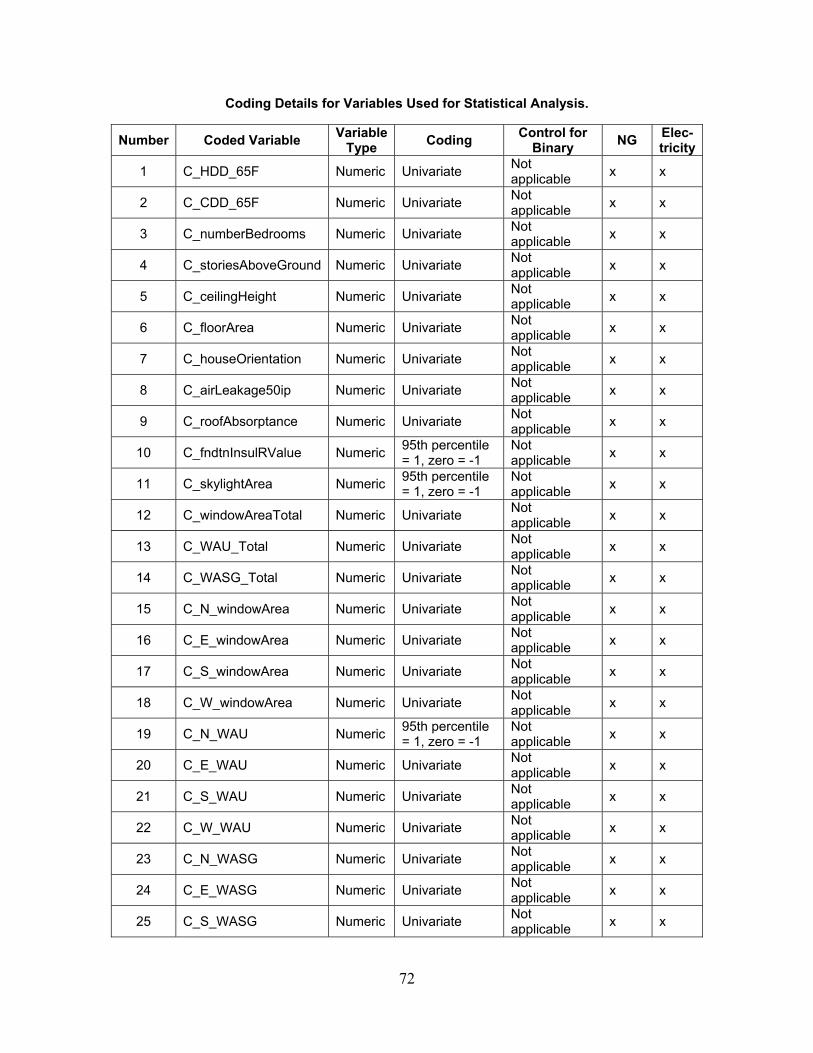
72

Coding Details for Variables Used for Statistical Analysis.

Number Coded Variable Variable

Type Coding

Control for Binary

NG Elec-tricity

1 C_HDD_65F Numeric Univariate Not applicable

x x

2 C_CDD_65F Numeric Univariate Not applicable

x x

3 C_numberBedrooms Numeric Univariate Not applicable

x x

4 C_storiesAboveGround Numeric Univariate Not applicable

x x

5 C_ceilingHeight Numeric Univariate Not applicable

x x

6 C_floorArea Numeric Univariate Not applicable

x x

7 C_houseOrientation Numeric Univariate Not applicable

x x

8 C_airLeakage50ip Numeric Univariate Not applicable

x x

9 C_roofAbsorptance Numeric Univariate Not applicable

x x

10 C_fndtnInsulRValue Numeric 95th percentile = 1, zero = -1

Not applicable

x x

11 C_skylightArea Numeric 95th percentile = 1, zero = -1

Not applicable

x x

12 C_windowAreaTotal Numeric Univariate Not applicable

x x

13 C_WAU_Total Numeric Univariate Not applicable

x x

14 C_WASG_Total Numeric Univariate Not applicable

x x

15 C_N_windowArea Numeric Univariate Not applicable

x x

16 C_E_windowArea Numeric Univariate Not applicable

x x

17 C_S_windowArea Numeric Univariate Not applicable

x x

18 C_W_windowArea Numeric Univariate Not applicable

x x

19 C_N_WAU Numeric 95th percentile = 1, zero = -1

Not applicable

x x

20 C_E_WAU Numeric Univariate Not applicable

x x

21 C_S_WAU Numeric Univariate Not applicable

x x

22 C_W_WAU Numeric Univariate Not applicable

x x

23 C_N_WASG Numeric Univariate Not applicable

x x

24 C_E_WASG Numeric Univariate Not applicable

x x

25 C_S_WASG Numeric Univariate Not applicable

x x

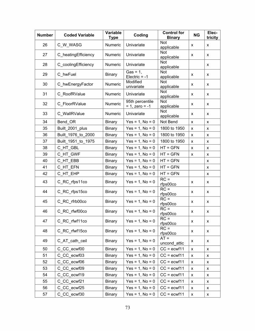
73

Number Coded Variable Variable

Type Coding

Control for Binary

NG Elec-tricity

26 C_W_WASG Numeric Univariate Not applicable

x x

27 C_heatingEfficiency Numeric Univariate Not applicable

x x

28 C_coolingEfficiency Numeric Univariate Not applicable

x

29 C_hwFuel Binary Gas = 1, Electric = -1

Not applicable

x x

30 C_hwEnergyFactor Numeric Modified univariate

Not applicable

x x

31 C_RoofRValue Numeric Univariate Not applicable

x x

32 C_FloorRValue Numeric 95th percentile = 1, zero = -1

Not applicable

x x

33 C_WallRValue Numeric Univariate Not applicable

x x

34 Bend_OR Binary Yes = 1, No = 0 Not Bend x x

35 Built_2001_plus Binary Yes = 1, No = 0 1800 to 1950 x x

36 Built_1976_to_2000 Binary Yes = 1, No = 0 1800 to 1950 x x

37 Built_1951_to_1975 Binary Yes = 1, No = 0 1800 to 1950 x x

38 C_HT_GBL Binary Yes = 1, No = 0 HT = GFN x x

39 C_HT_GWF Binary Yes = 1, No = 0 HT = GFN x x

40 C_HT_EBB Binary Yes = 1, No = 0 HT = GFN x

41 C_HT_EFN Binary Yes = 1, No = 0 HT = GFN x

42 C_HT_EHP Binary Yes = 1, No = 0 HT = GFN x

43 C_RC_rfps11co Binary Yes = 1, No = 0 RC = rfps00co

x x

44 C_RC_rfps15co Binary Yes = 1, No = 0 RC = rfps00co

x x

45 C_RC_rfrb00co Binary Yes = 1, No = 0 RC = rfps00co

x x

46 C_RC_rfwf00co Binary Yes = 1, No = 0 RC = rfps00co

x x

47 C_RC_rfwf11co Binary Yes = 1, No = 0 RC = rfps00co

x x

48 C_RC_rfwf15co Binary Yes = 1, No = 0 RC = rfps00co

x x

49 C_AT_cath_ceil Binary Yes = 1, No = 0 AT = uncond_attic

x x

50 C_CC_ecwf00 Binary Yes = 1, No = 0 CC = ecwf11 x x

51 C_CC_ecwf03 Binary Yes = 1, No = 0 CC = ecwf11 x x

52 C_CC_ecwf06 Binary Yes = 1, No = 0 CC = ecwf11 x x

53 C_CC_ecwf09 Binary Yes = 1, No = 0 CC = ecwf11 x x

54 C_CC_ecwf19 Binary Yes = 1, No = 0 CC = ecwf11 x x

55 C_CC_ecwf21 Binary Yes = 1, No = 0 CC = ecwf11 x x

56 C_CC_ecwf25 Binary Yes = 1, No = 0 CC = ecwf11 x x

57 C_CC_ecwf30 Binary Yes = 1, No = 0 CC = ecwf11 x x

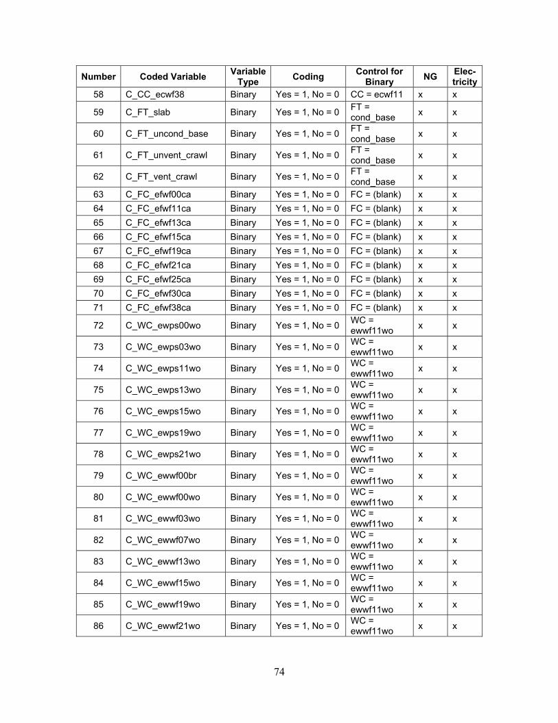
74

Number Coded Variable Variable

Type Coding

Control for Binary

NG Elec-tricity

58 C_CC_ecwf38 Binary Yes = 1, No = 0 CC = ecwf11 x x

59 C_FT_slab Binary Yes = 1, No = 0 FT = cond_base

x x

60 C_FT_uncond_base Binary Yes = 1, No = 0 FT = cond_base

x x

61 C_FT_unvent_crawl Binary Yes = 1, No = 0 FT = cond_base

x x

62 C_FT_vent_crawl Binary Yes = 1, No = 0 FT = cond_base

x x

63 C_FC_efwf00ca Binary Yes = 1, No = 0 FC = (blank) x x

64 C_FC_efwf11ca Binary Yes = 1, No = 0 FC = (blank) x x

65 C_FC_efwf13ca Binary Yes = 1, No = 0 FC = (blank) x x

66 C_FC_efwf15ca Binary Yes = 1, No = 0 FC = (blank) x x

67 C_FC_efwf19ca Binary Yes = 1, No = 0 FC = (blank) x x

68 C_FC_efwf21ca Binary Yes = 1, No = 0 FC = (blank) x x

69 C_FC_efwf25ca Binary Yes = 1, No = 0 FC = (blank) x x

70 C_FC_efwf30ca Binary Yes = 1, No = 0 FC = (blank) x x

71 C_FC_efwf38ca Binary Yes = 1, No = 0 FC = (blank) x x

72 C_WC_ewps00wo Binary Yes = 1, No = 0 WC = ewwf11wo

x x

73 C_WC_ewps03wo Binary Yes = 1, No = 0 WC = ewwf11wo

x x

74 C_WC_ewps11wo Binary Yes = 1, No = 0 WC = ewwf11wo

x x

75 C_WC_ewps13wo Binary Yes = 1, No = 0 WC = ewwf11wo

x x

76 C_WC_ewps15wo Binary Yes = 1, No = 0 WC = ewwf11wo

x x

77 C_WC_ewps19wo Binary Yes = 1, No = 0 WC = ewwf11wo

x x

78 C_WC_ewps21wo Binary Yes = 1, No = 0 WC = ewwf11wo

x x

79 C_WC_ewwf00br Binary Yes = 1, No = 0 WC = ewwf11wo

x x

80 C_WC_ewwf00wo Binary Yes = 1, No = 0 WC = ewwf11wo

x x

81 C_WC_ewwf03wo Binary Yes = 1, No = 0 WC = ewwf11wo

x x

82 C_WC_ewwf07wo Binary Yes = 1, No = 0 WC = ewwf11wo

x x

83 C_WC_ewwf13wo Binary Yes = 1, No = 0 WC = ewwf11wo

x x

84 C_WC_ewwf15wo Binary Yes = 1, No = 0 WC = ewwf11wo

x x

85 C_WC_ewwf19wo Binary Yes = 1, No = 0 WC = ewwf11wo

x x

86 C_WC_ewwf21wo Binary Yes = 1, No = 0 WC = ewwf11wo

x x

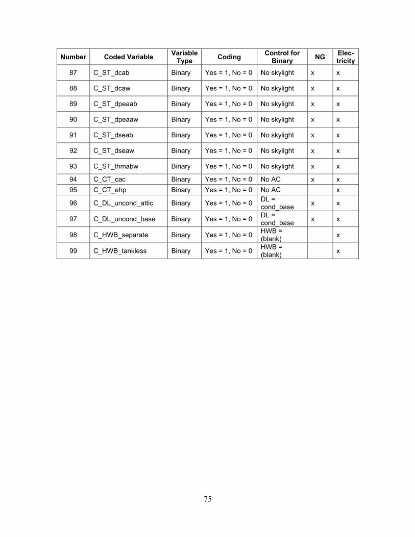
75

Number Coded Variable Variable

Type Coding

Control for Binary

NG Elec-tricity

87 C_ST_dcab Binary Yes = 1, No = 0 No skylight x x

88 C_ST_dcaw Binary Yes = 1, No = 0 No skylight x x

89 C_ST_dpeaab Binary Yes = 1, No = 0 No skylight x x

90 C_ST_dpeaaw Binary Yes = 1, No = 0 No skylight x x

91 C_ST_dseab Binary Yes = 1, No = 0 No skylight x x

92 C_ST_dseaw Binary Yes = 1, No = 0 No skylight x x

93 C_ST_thmabw Binary Yes = 1, No = 0 No skylight x x

94 C_CT_cac Binary Yes = 1, No = 0 No AC x x

95 C_CT_ehp Binary Yes = 1, No = 0 No AC x

96 C_DL_uncond_attic Binary Yes = 1, No = 0 DL = cond_base

x x

97 C_DL_uncond_base Binary Yes = 1, No = 0 DL = cond_base

x x

98 C_HWB_separate Binary Yes = 1, No = 0 HWB = (blank)

x

99 C_HWB_tankless Binary Yes = 1, No = 0 HWB = (blank)

x

76

Appendix F Statistical Equations The table below shows the mathematical equations used to populate Table 1 and Table 2 in Section 2.

Statistic Description Equation

Number of Observations The number of observations in sample

Mean Measured The mean value of the measured

observations ∑

Mean Predicted The mean value of the predicted

observations ∑

Difference Differences between predicted and measured observations ( )

−

Mean Difference The mean value of the differences between predicted and measured

observations ( ̅)

∑ ( − )

Median Difference The median value of the differences between predicted and measured

observations

The value for which 50% of errors are lower and 50% are

higher.

Standard Deviation of Difference

The sample standard deviation of the differences

1− 1 ( − ̅)

Mean Absolute Difference The mean value of the absolute

differences ∑ | |

Median Absolute Difference

The median value of the absolute differences

The value for which 50% of errors are lower and 50% are

higher.

Mean Absolute Percent Difference

The mean value of the absolute differences

∑

Median Absolute Percent Difference

The median value of the absolute differences

The value for which 50% of errors are lower and 50% are

higher.

Root Mean Squared Error (RMSE)

The square root of the mean value of the squared differences = ∑

Percent Root Mean Square Error

Normalized square root of the mean value of the squared differences = × 100