sustainability

Article

Assessment of the Bearing Capacity of Foundations onRock Masses Subjected to Seismic and Seepage Loads

Rubén Galindo 1,* , Ana Alencar 1, Nihat Sinan Isik 2 and Claudio Olalla Marañón 1

1 Departamento de Ingeniería y Morfología del Terreno, Universidad Politécnica de Madrid,28040 Madrid, Spain; at.santos@alumnos.upm.es (A.A.); claudio.olalla@upm.es (C.O.M.)

2 Department of Civil Engineering, Faculty of Technology, Gazi University, 06560 Ankara, Turkey;nihatsinan@gazi.edu.tr

* Correspondence: rubenangel.galindo@upm.es

Received: 20 October 2020; Accepted: 30 November 2020; Published: 2 December 2020�����������������

Abstract: It is usual to adopt the seismic force acting as an additional body force, employing thepseudo-static hypothesis, when considering earthquakes in the estimation of the bearing capacityof foundations. A similar approach in seepage studies can be applied for the pore pressure’sconsideration as an external force. In the present study, the bearing capacity of shallow foundationson rock masses considering the presence of the pseudo-static load was developed by applying ananalytical solution for the Modified Hoek and Brown failure criterion. Calculations were performedadopting various inclinations of the load and the slope on the edge of the foundation, as well asdifferent values of the vertical and horizontal components of the pseudo-static load. The results arepresented in the form of charts to allow an affordable and immediate practical application for footingproblems in the event of seismic loads or seepages. Finally, and to validate the analytical solutionpresented, a numerical study was developed applying the finite difference method to estimate thebearing capacity of a shallow foundation on a rock mass considering the presence of an additionalhorizontal force that could be caused by an earthquake or a seepage.

Keywords: Hoek–Brown criterion; seismic load; seepage; analytical method; pseudo-static load;finite difference method

1. Introduction

Natural events such as earthquakes and floods generate impulsive loads and seepages in theground, endangering civil constructions. Infrastructures must be built to resist natural risks in adequatesafety conditions and be economically viable. Therefore, an optimized design that reliably considersthe negative effects that these natural phenomena introduce to the foundations is highly advisable toguarantee the sustainability of the infrastructures.

Today, research in the area of seismic bearing capacity is very much in demand because ofthe devastating effects of foundations under earthquake conditions. A high number of failureshave occurred where field conditions have indicated that the bearing capacity was reduced duringseismic events.

In the estimation of the bearing capacity, when the effect of the earthquake is considered, it isusual to adopt the pseudo-static hypothesis where the seismic force acts as an additional body forcewithin the soil mass. The vertical and horizontal acceleration are applied both on the ground and in thestructure. Thus, the limit conditions can be evaluated by introducing pseudo-static equivalent forces,corresponding with the inertial forces in the soil during the seismic excitation. Such an approach isbased on the hypothesis of a synchronous motion for the soil underneath the footing, a hypothesis thatis acceptable only in the case of small footing widths and large values for the soil stiffness. According to

Sustainability 2020, 12, 10063; doi:10.3390/su122310063 www.mdpi.com/journal/sustainability

Sustainability 2020, 12, 10063 2 of 21

numerous studies carried out about this issue in the field of geotechnical engineering, it is known thatthe bearing capacity is considerably reduced mostly due to the horizontal component.

These studies are primarily based on (a) the limit equilibrium method [1–4], (b) the method of thecharacteristics [5], and (c) the limit analysis method using numerical analysis [6–8].

Limit equilibrium methods have evolved and incorporated different factors, generalizing theapplication hypotheses to solve the most general possible configurations. Thus, Sarma and Iossifelis [1]determined seismic bearing capacity factors for soils with seismic acceleration acting on the structureonly and using the limit equilibrium technique of slope stability analysis with inclined slices.Later, Richarts et al. [2] considered the inertial mass of the ground using a simplification of thePrandtl failure surface to eliminate the fan-shaped transition zone and thereby average its effectconcentration. This effect can be considered as a retaining wall with the active lateral thrust fromthe region below the foundation pushing against the passive resistance from the external region.Then, Choudhury and Rao [4], using the limit equilibrium method, studied the seismic forces forshallow strip footings embedded in sloping ground with a linear failure criterion. They consideredpseudo-static forces acting both on the footing and on the soil below the footing and considered in theanalysis a composite failure surface involving a planar and logspiral.

For its part, Kumar and Rao [5] applied the method of the characteristics using pseudo-static forcesfor a Mohr–Coulomb criterion. The analytical methods were limited to simplified configurations wherethe inertia of the soil mass was not included and had to be completed with empirical or numerical terms.

Adopting the conventional pseudo-static approach, Yang [7] used a non-linear failure criterionto evaluate the seismic bearing capacity of strip foundations on rock slopes by means of thegeneralized tangential technique, in which the non-linear strength is replaced by an “optimal”tangential Mohr–Coulomb domain in a limit analysis framework where the upper-bound solutions areobtained by optimization.

A numerical study was performed by Raj et al. [8] using finite-element limit analysis for shallowstrip foundations embedded in homogeneous soil slopes, applying a pseudo-static approach to considerthe seismic action on both the soil and foundation.

Nova and Montrasio [9] introduced a satisfactory description of the dynamic soil–structureinteraction by means of the macro-element concept (the system as a unique, non-linear macro-elementwith a limited number of degrees of freedom), which has been applied by many researchers to differentproblems of shallow foundations [10,11].

Applying a similar approach, in recent years, studies have been published where the porepressure has been included as an external force, analyzing the slope stability in soil [12] and rock [13],and affecting the bearing capacity of the shallow foundation on soil [14–16] and in jointed rock mass [17].In foundations with large widths such as dams, the seepage tends to present an almost horizontal flowin the influence area of the foundation, as has been possible to verify in real cases [18].

In the case of seismic load, the horizontal acceleration is the same in the whole model, while inthe case of seepage, the horizontal acceleration can vary once there is a loss of force along the waterpath. Depending on the direction of the groundwater flow, it can act as a passive (resistant) or activeforce [16], once it is in the same direction to the stress path or not. Thus, the wedge formed belowthe footing is asymmetric. Additionally, Veiskarami and Kumar [14] show that with an increasein the hydraulic gradient, the nature of the failure patterns becomes more non-symmetrical; for anon-symmetrical failure pattern, the footing would have a greater chance of failing in overturningrather than under simple vertical compression.

It must be pointed out that the traditional formulations of the bearing capacity are based on theMohr–Coulomb parameters (the cohesion and friction angle) that are very efficient in the field of soilmechanics, with a linear behavior. In rock mechanics, the current methods for estimating the bearingcapacity adopt the Hoek and Brown failure criterion [19] (valid only for rock masses not excessivelyfractured) and Modified Hoek and Brown failure criterion [20,21] (valid under general conditions ofdegree of fracturing of the rock mass). Both failure criteria are non-linear and applicable to the rock

Sustainability 2020, 12, 10063 3 of 21

mass with a homogeneous and isotropic behavior. The linearization of the failure criterion impliesincorporating approximate methods and requires iterative procedures to ensure an optimized upperor lower bound for the solution; therefore, it is desirable to be able to address the problem using thenon-linear criterion directly.

In addition, most of the formulations are limited to flat ground, the need to analyze the bearingcapacity of shallow foundations on sloping ground of moderate slopes being very common in damand bridge foundations. Finally, although the numerical solutions allow solving complex problemswith singular considerations when a seismic load or filtration acts, in the face of non-linear criteria,a complete analysis of numerical convergence is necessary, which complicates the practical applicabilityand the rapid design of foundations in rock masses.

An analytical method for the calculation of shallow foundations that solves the internal equilibriumequations and boundary conditions combined with the failure criterion was proposed by Serrano andOlalla [22] and Serrano et al. [23], applying the Hoek and Brown [19] and the Modified Hoek andBrown failure criterion [20], respectively. It is based on the characteristic lines method [24], with thehypothesis of the weightless rock, strip foundation and associative flow law. The formulation of thebearing capacity proposed by Serrano et al. [23] introduces a bearing capacity factor, which makes thefailure pressure proportional to the uniaxial compressive strength of the rock (UCS).

In the present study, the analytical formulation of Serrano et al. [23] and design charts weredeveloped to study the bearing capacity when there is an increase in load induced by forces of seismicorigin or filtration in rock masses, where it is necessary to use a non-linear failure criterion and theown weight of the ground is generally negligible compared to the resistant components, considering,as usual, the possibility of the inclination of the ground to the edge of the foundation. Besides,a numerical model was created through a finite difference method, assuming a similar hypothesisfor the analytical solution, and it was observed that the results obtained by both methods werequite similar.

2. Problem Statement

2.1. Mathematical Model

As is generally known, in rock mechanics, the non-linear Modified Hoek and Brown failurecriterion is the most used, and it is applicable for a rock mass with a homogeneous and isotropicbehavior, meaning that by the inexistence or by the abundance of discontinuities, it has the samephysical properties in all directions.

In this research, the Modified Hoek and Brown failure criterion [21,25] was used, and it wasformulated as a function of the major principal stress (σ3) and minor principal stress (σ1) according tothe following equation:

σ1 − σ3

σc=

(m·σ3

σc+ s

)a(1)

The uniaxial compressive strength (UCS) is σc, while the parameters m, s and a can be evaluatedwith (2)–(4) and depend on the intact rock parameter (mo), quality index of the rock mass (geologicalstrength index (GSI)) and damage in the rock mass due to human actions (D), which in shallowfoundations, is usually equal to zero.

m = mo·eGSI−10028−14·D (2)

s = eGSI−100

9−3·D (3)

a =12+

16

(e−GSI

15 − e−20

3

)(4)

Serrano et al. [23] proposed an analytical formulation for estimating the ultimate bearing capacityof the strip footing for a weightless rock mass, based on the characteristic method, which allows solvingthe internal equilibrium equations in a continuous medium together with the boundary equations and

Sustainability 2020, 12, 10063 4 of 21

those that define the failure criterion. This solution is based on the Modified Hoek and Brown failurecriterion [20], taking into account the associated plastic flow rule.

According to this analytical formulation, the ground surface that supports the foundation iscomposed of two sectors (Figure 1): Boundary 1 (free), with the inclination i1, where the load actingon a surface is known (for example, the self-weight load on the foundation level or the load frominstalled anchors), and Boundary 2 (foundation), where the bearing capacity of the foundation shouldbe determined (acting with the inclination of i2).

Sustainability 2020, 11, x FOR PEER REVIEW 4 of 22

Serrano et al. [23] proposed an analytical formulation for estimating the ultimate bearing

capacity of the strip footing for a weightless rock mass, based on the characteristic method, which

allows solving the internal equilibrium equations in a continuous medium together with the

boundary equations and those that define the failure criterion. This solution is based on the

Modified Hoek and Brown failure criterion [20], taking into account the associated plastic flow rule.

According to this analytical formulation, the ground surface that supports the foundation is

composed of two sectors (Figure 1): Boundary 1 (free), with the inclination i1, where the load acting

on a surface is known (for example, the self-weight load on the foundation level or the load from

installed anchors), and Boundary 2 (foundation), where the bearing capacity of the foundation

should be determined (acting with the inclination of i2).

Figure 1. Mathematical model of the bearing capacity of the strip footing.

The solution based on the characteristic lines method requires the equation of the Riemann

invariants (Ia) [26] fulfilled along the characteristic line:

𝐼𝑎(𝜌1) + 𝜓1 = 𝐼𝑎(𝜌2) + 𝜓2 (5)

𝐼𝑎(𝜌) =1

2 ∙ 𝑘∙ [𝑐𝑜𝑡𝑔(𝜌) + 𝑙𝑛 (𝑐𝑜𝑡𝑔 (

𝜌

2))] (6)

In this equation, the instantaneous friction angle at the boundary 2 (ρ2) is the only unknown,

because the other variables can be defined at Boundary 1: the instantaneous friction angle at

1

Ph Boundary 1: Free surface

Boundary 2: Foundation

Rankine-1 region

Rankine-2 region

Prandtl region

(𝜋

4+

𝜌2

2)

(𝜋

4−

𝜌1

2)

i1 i2

Figure 1. Mathematical model of the bearing capacity of the strip footing.

The solution based on the characteristic lines method requires the equation of the Riemanninvariants (Ia) [26] fulfilled along the characteristic line:

Ia(ρ1) +ψ1 = Ia(ρ2) +ψ2 (5)

Ia(ρ) =1

2·k·

[cotg(ρ) + ln

(cotg

(ρ2

))](6)

In this equation, the instantaneous friction angle at the boundary 2 (ρ2) is the only unknown,because the other variables can be defined at Boundary 1: the instantaneous friction angle at Boundary1 (ρ1) and the angle (Ψ1) between the major principal stress and the vertical axis in this sector (Figure 1).

Sustainability 2020, 12, 10063 5 of 21

Thus, expressing Ψ2 (the angle between the major principal stress and the vertical axis in Boundary 2,as indicated in Figure 1) as a function of ρ2, it is possible to estimate the ultimate bearing capacity.

Through the analytical method [23], the bearing capacity was obtained by (7).

Ph = βa·(Nβ − ζa

)(7)

The resistant parameters βa and ζa were applied to make dimensionless the calculation of theModified Hoek and Brown failure criterion. βa represents the characteristic strength, which has thesame units as the UCS and was used to make the pressures dimensionless, while ζa (the “tenacitycoefficient”) is a dimensionless coefficient that, multiplied by βa, corresponds to the tensile strength.

βa = Aa·UCS; ζa =s

(m·Aa); Aa =

(m·(1− a)

21a

) 1k

; k =(1− a)

a(8)

Aa, k and the exponent a are constants for the rock mass and depend on the rock type (m),UCS and GSI.

Nβ is the bearing capacity factor, and it can be calculated, according to the problem statement,as follows.

The angle of internal friction (ρ1) can be obtained by iteration from the load at Boundary 1.From the value of ρ1 and by the iteration of (5), the value of the internal friction angle at Boundary 2(ρ2) can be calculated.

Finally, knowingρ2, the bearing capacity factor (Nβ) can be calculated, and using, again, parametersβa and ζa, the ultimate bearing capacity (Ph) was estimated as an expression that depended on theinstantaneous friction angle at Boundary 2 (ρ2), the inclination of the load on the foundation (i2) andthe exponent of the Modified Hoek and Brown criterion (a; k = (1 − a)/a):

Nβ = cos(i2)(

1−sin(ρ2)

k·sin(ρ2)

) 1k(

a·(1+sin(ρ2))

sin(ρ2)cos(i2)

+

√1−

[a·(1+k·sin(ρ2))

sin(ρ2)sin(i2)

]2 (9)

2.2. Consideration of Pseudo-Static Load: Mathematical Transformation

In the pseudo-static approach, static horizontal and vertical inertial forces, which are intendedto represent the destabilizing effects of the earthquake or seepage, are calculated as the product ofthe seismic/seepage coefficients and the distributed load applied to the boundaries. In the case of therock mass, the weight collaboration is usually negligible compared to the resistance of the ground,and therefore, the inertial forces are applied both to the foundation and to the free boundary.

The vertical seismic/seepage coefficient kv is supposed to be a fraction of one horizontal kh, and inparticular, the vertical acceleration is thus assumed to be in phase with the horizontal acceleration.

The present study is divided into three parts: (a) The first one considered the horizontal (kh) andvertical (kv) components of the pseudo-static load on both boundaries, with a free boundary inclinedby α at the edge of the foundation, which resembles the hypothesis of a seism. (b) In the second part,only the horizontal component (kh) on the foundation boundary was adopted (it being possible toconsider both the horizontal and vertical components on the free boundary depending on the directionof the seepage), with the free boundary inclined by α at the edge of the foundation. This hypothesis ismore similar to the presence of a seepage (both hypotheses are represented schematically in Figure 2,and they are solved and shown in new charts including additional horizontal and vertical loads).(c) The final section is the comparison of the analytical result with that obtained numerically throughthe finite difference method.

Sustainability 2020, 12, 10063 6 of 21

Sustainability 2020, 11, x FOR PEER REVIEW 6 of 22

Figure 2. Scheme of the pseudo-static load acting: (a) Seismic load (Fs); (b) Seepage (Fw).

The application of the analytical method [23] with an increase in the horizontal and/or vertical

loads produced by inertial forces can be carried out by means of a parametric transformation from

the incidence angles of the loads in the static configuration to the final configuration including the

seismic or seepage loads. Thus, for a general case of a pseudo-static force on the two boundaries, the

starting point is the load acting in the static hypothesis (subscript 0), as is represented in Figure 3a. In

this case, the inclinations of the load on the foundation (p) and of the load on the free boundary (q)

are 𝑖02 and 𝑖01, respectively. However, considering the pseudo-static load, the inclinations of the

loads in both boundaries are different (i2 for the foundation boundary and i1 for the free boundary).

Figure 3b allows the deduction of the mathematical transformations of these angles from the static

configuration to the final pseudo-static configuration as a function of the angle (α) of the free

boundary and of the horizontal (kh1 or kh2, depending on the boundary) and vertical (kv1 or kv2,

depending on the boundary) components of the pseudo-static load. These transformations are

expressed in (10) and (11).

𝑡𝑎𝑛 (𝑖2) = 𝑡𝑎𝑛 (𝑖02) + 𝑘ℎ2

1 − 𝑘𝑣2 (10)

𝑡𝑎𝑛 ( + 𝑖1) = (1 − 𝑘𝑣1)𝑡𝑎𝑛(𝛼 + 𝑖01)

1 − 𝑘ℎ1𝑡𝑎𝑛(𝛼 + 𝑖01) (11)

Boundary 2 (Foundation) Boundary 1 (Free)

pv

ph qv

qh

a i01 i02

Figure 2. Scheme of the pseudo-static load acting: (a) Seismic load (Fs); (b) Seepage (Fw).

The application of the analytical method [23] with an increase in the horizontal and/or verticalloads produced by inertial forces can be carried out by means of a parametric transformation fromthe incidence angles of the loads in the static configuration to the final configuration including theseismic or seepage loads. Thus, for a general case of a pseudo-static force on the two boundaries,the starting point is the load acting in the static hypothesis (subscript 0), as is represented in Figure 3a.In this case, the inclinations of the load on the foundation (p) and of the load on the free boundary(q) are i02 and i01, respectively. However, considering the pseudo-static load, the inclinations of theloads in both boundaries are different (i2 for the foundation boundary and i1 for the free boundary).Figure 3b allows the deduction of the mathematical transformations of these angles from the staticconfiguration to the final pseudo-static configuration as a function of the angle (α) of the free boundaryand of the horizontal (kh1 or kh2, depending on the boundary) and vertical (kv1 or kv2, depending on theboundary) components of the pseudo-static load. These transformations are expressed in (10) and (11).

tan (i2) =tan (i02) + kh2

1 − kv2(10)

tan (α+ i1) =(1− kv1)tan(α+ i01)

1− kh1tan(α+ i01)(11)

Therefore, for the pseudo-static calculation, the analytical formulation of the characteristicsmethod expressed by (5) can be used using the load inclinations on each boundary obtained throughthe transformations indicated in Equations (10) and (11) as a function of the horizontal and verticalcomponents of the added inertial load and of the angle of inclination of Boundary 1.

In the case of the seismic load, it is considered that kh1 = kh2 and kv1 = kv2, while in the case of theseepage load, kv1 = 0; thus, for clearer notation, it is denoted that for the seismic load, the horizontaland vertical components of the pseudo-static load are kh and kv, respectively, and for the seepage load,the horizontal component of the pseudo-static load on the foundation boundary is called ia.

Sustainability 2020, 12, 10063 7 of 21

Sustainability 2020, 11, x FOR PEER REVIEW 6 of 22

Figure 2. Scheme of the pseudo-static load acting: (a) Seismic load (Fs); (b) Seepage (Fw).

The application of the analytical method [23] with an increase in the horizontal and/or vertical

loads produced by inertial forces can be carried out by means of a parametric transformation from

the incidence angles of the loads in the static configuration to the final configuration including the

seismic or seepage loads. Thus, for a general case of a pseudo-static force on the two boundaries, the

starting point is the load acting in the static hypothesis (subscript 0), as is represented in Figure 3a. In

this case, the inclinations of the load on the foundation (p) and of the load on the free boundary (q)

are 𝑖02 and 𝑖01, respectively. However, considering the pseudo-static load, the inclinations of the

loads in both boundaries are different (i2 for the foundation boundary and i1 for the free boundary).

Figure 3b allows the deduction of the mathematical transformations of these angles from the static

configuration to the final pseudo-static configuration as a function of the angle (α) of the free

boundary and of the horizontal (kh1 or kh2, depending on the boundary) and vertical (kv1 or kv2,

depending on the boundary) components of the pseudo-static load. These transformations are

expressed in (10) and (11).

𝑡𝑎𝑛 (𝑖2) = 𝑡𝑎𝑛 (𝑖02) + 𝑘ℎ2

1 − 𝑘𝑣2 (10)

𝑡𝑎𝑛 ( + 𝑖1) = (1 − 𝑘𝑣1)𝑡𝑎𝑛(𝛼 + 𝑖01)

1 − 𝑘ℎ1𝑡𝑎𝑛(𝛼 + 𝑖01) (11)

Boundary 2 (Foundation) Boundary 1 (Free)

pv

ph qv

qh

a i01 i02

Sustainability 2020, 11, x FOR PEER REVIEW 7 of 22

Figure 3. Scheme of the seismic load estimation: (a) static configuration and (b) pseudo-static

inclination on Boundary 1 (external boundary of foundation). Note: In this figure, the subscripts “v”

and “h” refer to the vertical and horizontal projections of the load.

Therefore, for the pseudo-static calculation, the analytical formulation of the characteristics

method expressed by (5) can be used using the load inclinations on each boundary obtained through

the transformations indicated in Equations (10) and (11) as a function of the horizontal and vertical

components of the added inertial load and of the angle of inclination of Boundary 1.

In the case of the seismic load, it is considered that kh1 = kh2 and kv1 = kv2, while in the case of the

seepage load, kv1 = 0; thus, for clearer notation, it is denoted that for the seismic load, the horizontal

and vertical components of the pseudo-static load are kh and kv, respectively, and for the seepage

load, the horizontal component of the pseudo-static load on the foundation boundary is called ia.

3. Design Charts for Estimation of Bearing Capacity

3.1. Calculation Cases and Representation of Analytical Results

Once the mathematical transformation of the load angles in the boundaries, for the problem

presented in Figure 3a, according to (10) and (11) for the seismic and seepage load has been carried

out, the analytical formulation using the method of the characteristic lines can be applied. The

results are presented as graphs, which allow the estimation of the bearing capacity considering the

presence of a pseudo-static load.

The charts are clustered according to the exponent “a” of the Modified Hoek and Brown

criterion, the inclination α of Boundary 1 and kv of the foundation boundary, and they were

developed based on io2 and the horizontal component of the pseudo-static load of the foundation

boundary (kh). It is noted that for high confining pressures in Boundary 1, it is not always possible to

obtain a bearing capacity value; this limit is demarcated by the non-equilibrium line.

For the development of the new charts, three values of the GSI (geological strength index) were

adopted (8, 20 and 100), which generated exponents “a” of the Modified Hoek and Brown criterion

equal to 0.5, 0.55 and 0.6 from (4). Based on (7), the values of the rock type (mo) and the uniaxial

compressive strength of the rock (UCS) do not influence the normalized graphs, and to perform the

calculations, mo = 15 and UCS = 1 MPa were adopted.

In the graphs developed for kv > 0 on the foundation boundary, representative of the seismic

load, four kh values were adopted and correlated two values of kv, two slope angles for the free

boundary (α) and three initial inclination angles for the load on the foundation boundary (io2),

representing the inclination angle of the load without considering the pseudo-static load. In Table 1,

the values used in the analysis are indicated.

𝑡𝑎𝑛 (𝑖2) = 𝑝ℎ +𝑘ℎ 2·𝑝𝑣

(1 − 𝑘𝑣2) 𝑝𝑣 𝑡𝑎𝑛 (

𝜋

2− − 𝑖1) =

𝑞ℎ −𝑘ℎ 1·𝑞𝑣

(1 − 𝑘𝑣1) 𝑞𝑣

Boundary 2 (Foundation) Boundary 1 (Free)

pv-kv2pv

ph+kh2pv qv-kv1qv

qh-kh1qv

b

Figure 3. Scheme of the seismic load estimation: (a) static configuration and (b) pseudo-static inclinationon Boundary 1 (external boundary of foundation). Note: In this figure, the subscripts “v” and “h” referto the vertical and horizontal projections of the load.

3. Design Charts for Estimation of Bearing Capacity

3.1. Calculation Cases and Representation of Analytical Results

Once the mathematical transformation of the load angles in the boundaries, for the problempresented in Figure 3a, according to (10) and (11) for the seismic and seepage load has been carried out,the analytical formulation using the method of the characteristic lines can be applied. The results arepresented as graphs, which allow the estimation of the bearing capacity considering the presence of apseudo-static load.

The charts are clustered according to the exponent “a” of the Modified Hoek and Brown criterion,the inclination α of Boundary 1 and kv of the foundation boundary, and they were developed based onio2 and the horizontal component of the pseudo-static load of the foundation boundary (kh). It is notedthat for high confining pressures in Boundary 1, it is not always possible to obtain a bearing capacityvalue; this limit is demarcated by the non-equilibrium line.

For the development of the new charts, three values of the GSI (geological strength index) wereadopted (8, 20 and 100), which generated exponents “a” of the Modified Hoek and Brown criterionequal to 0.5, 0.55 and 0.6 from (4). Based on (7), the values of the rock type (mo) and the uniaxial

Sustainability 2020, 12, 10063 8 of 21

compressive strength of the rock (UCS) do not influence the normalized graphs, and to perform thecalculations, mo = 15 and UCS = 1 MPa were adopted.

In the graphs developed for kv > 0 on the foundation boundary, representative of the seismic load,four kh values were adopted and correlated two values of kv, two slope angles for the free boundary(α) and three initial inclination angles for the load on the foundation boundary (io2), representing theinclination angle of the load without considering the pseudo-static load. In Table 1, the values used inthe analysis are indicated.

Table 1. Geometric parameters adopted in the model (kv > 0).

kh kv = kh, kh/2 α (◦) io2 (◦) a

0.1 0.1, 0.05

0, 20 0, 10, 200.5,

0.55,0.6

0.2 0.2, 0.10.3 0.3, 0.150.4 0.4, 0.2

On the other hand, in the charts developed with kv = 0 on the foundation boundary, representativeof the seepage loads, three values of horizontal load were used, in those cases called ia (additionalinclination); three values of the slope (α) and another three values of io2 were also used, which areshown in Table 2.

Table 2. Geometric parameters adopted in the model (kv = 0).

ia α (◦) io2 (◦) a

0.1, 0.2, 0.3 0, 5, 10 0, 10, 20 0.5, 0.55, 0.6

It is emphasized that kh (the horizontal component of the seismic load) and ia (the horizontalcomponent of the seepage load) were in proportion to the vertical load applied; the values expressedin Tables 1 and 2 are the relation between the horizontal and the vertical load. The final inclinationof the load in the foundation boundary, in the cases of seepage loads, can be obtained directly as asimplification of (10):

tan (i2) = tan(io2) + ia (12)

3.2. Charts for Estimation of Bearing Capacity Considering kh and kv > 0 (Seismic Case)

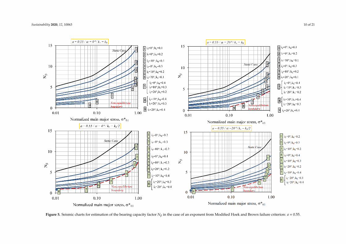
These design charts allow obtaining the bearing capacity factor Nβ (9), and they are presentedin Figures 4–6. Each graph represented corresponds to determined values of the exponent “a” ofthe Modified Hoek and Brown criterion of the rock mass (a function of the GSI of the quality ofthe rock mass), the inclination α of the free boundary and the ratio of the vertical and horizontalcomponents of the pseudo-static load (kv/kh = 1 or 0.5). In each graph, different curves correspondingto the angles of the inclination of the static load on Boundary 2 (io2) and horizontal component of thepseudo-static load (kh) are presented, so that in the abscissa, the known value of the normalized mainmajor stress is presented, normalized on Boundary 1 (σ*01), estimated through (13). It is dimensionlessand corresponds to the load acting on Boundary 1, and its value depends on the inclination angle ofthe load i1 obtained by (11) (Figure 1).

σ∗01 =σ1

βa+ ζa (13)

Among the graphs, it is easy to appreciate that as there is a greater slope for the free boundary (α),a lower kv/kh ratio and a lower exponent “a” from the Modified Hoek and Brown failure criterion,the value of Nβ follows a declining trend.

Sustainability 2020, 12, 10063 9 of 21Sustainability 2020, 11, x FOR PEER REVIEW 10 of 22

0

5

10

15

0,01 1,00

N

0,10

Normalized main major stress, *01

a = 0.5 / = 0 / kv = kh

i2=0; kh=0.1

i2=0; kh=0.2

i2=0; kh=0.3

i2=0; kh=0.4

i2=10; kh=0.1

i2=10; kh=0.2

i2=20; kh=0.1

i2=20; kh=0.2

i2=10; kh=0.3

i2=20; kh=0.4

i2=20; kh=0.3

i2=10; kh=0.4

1

1

2

2

3

3

4

4

5

5

6

6

7

7

8

8

9 9

Non-equilibrium

boundary

Static Case

0

5

10

15

0,01 0,10 1,00

N

Normalized main major stress, *01

a = 0.5 / = 20 / kv = kh

i2=0; kh=0.1

i2=0; kh=0.2

i2=0; kh=0.3

i2=0; kh=0.4

i2=10; kh=0.1

i2=10; kh=0.2

i2=20; kh=0.1

i2=20; kh=0.2

i2=10; kh=0.3

i2=20; kh=0.4

i2=20; kh=0.3

i2=10; kh=0.4

1

1

2

2

3

3

4

4

5

5

6

6

7

7

889

9

Non-equilibrium

boundary

Static Case

0

5

10

15

0,01 0.10 1.00

N

Normalized main major stress, *01

a = 0.5 / = 0 / kv = kh/2

i2=0; kh=0.2

i2=0; kh=0.3

i2=0; kh=0.4

i2=10; kh=0.2

i2=20; kh=0.2

i2=10; kh=0.3

i2=20; kh=0.4

i2=20; kh=0.3

i2=10; kh=0.4

1

1

2

2

3

3

4

4

5

5

6

6

7

7

8

8

Non-equilibrium

boundary

Static Case

0

5

10

15

0.01 1.00

N

0.10

Normalized main major stress, *01

a = 0.5 / =20 / kv = kh/2

i2=0; kh=0.2

i2=0; kh=0.3

i2=0; kh=0.4

i2=10; kh=0.2

i2=20; kh=0.2

i2=10; kh=0.3

i2=20; kh=0.4

i2=20; kh=0.3

i2=10; kh=0.4

1

1

2

2

3

3

4

4

5

5

6

6

7

7

8

8

Non-equilibrium boundary

Static Case

Figure 4. Seismic charts for estimation of the bearing capacity factor Nβ in the case of an exponent from Modified Hoek and Brown failure criterion: a = 0.5.

Sustainability 2020, 12, 10063 10 of 21Sustainability 2020, 11, x FOR PEER REVIEW 11 of 22

Figure 4. Seismic charts for estimation of the bearing capacity factor Nß in the case of an exponent from Modified Hoek and Brown failure criterion: a = 0.5.

Figure 5. Seismic charts for estimation of the bearing capacity factor Nß in the case of an exponent from Modified Hoek and Brown failure criterion: a = 0.55. Figure 5. Seismic charts for estimation of the bearing capacity factor Nβ in the case of an exponent from Modified Hoek and Brown failure criterion: a = 0.55.

Sustainability 2020, 12, 10063 11 of 21

Sustainability 2020, 11, x FOR PEER REVIEW 12 of 22

Figure 6. Seismic charts for estimation of the bearing capacity factor Nß in the case of an exponent from Modified Hoek and Brown failure criterion: a = 0.6. Figure 6. Seismic charts for estimation of the bearing capacity factor Nβ in the case of an exponent from Modified Hoek and Brown failure criterion: a = 0.6.

Sustainability 2020, 12, 10063 12 of 21

Table 3 shows the results of the bearing capacity (Ph) of some studied cases. It should be noted thatthe value of Ph is not directly proportional to Nβ, meaning that a higher value of Nβ does not necessarilymean that the value of Ph will be higher. Besides, the same value of Nβ is associated with differentvalues of Ph depending on the other geotechnical parameters, as shown in (7). On the other hand, it isobserved that under equal conditions (only varying the GSI and, consequently, the parameter “a”),the greater the GSI, the lower the value of Nβ; however, as expected, the bearing capacity of the rockmass is higher.

Table 3. Bearing capacity estimation by analytical method [23] (mo = 15 and uniaxial compressivestrength (UCS) = 1 MPa).

GSI a α (◦) σ*01 io2 (◦) kh kvβa

(MPa) ζa NβPh

(MPa)

8 0.6 0 0.1 0 0.2 0.2 0.1051 0.00062 6.31 0.66420 0.55 0 0.1 0 0.2 0.2 0.1309 0.00122 5.42 0.709

100 0.5 0 0.1 0 0.2 0.2 1.8750 0.03556 4.93 9.174

8 0.6 0 0.1 0 0.2 0.1 0.1051 0.00062 6.70 0.70420 0.55 0 0.1 0 0.2 0.1 0.1309 0.00122 5.73 0.750

100 0.5 0 0.1 0 0.2 0.1 1.8750 0.03556 5.21 9.698

8 0.6 0 0.1 10 0.2 0.2 0.1051 0.00062 3.77 0.39720 0.55 0 0.1 10 0.2 0.2 0.1309 0.00122 3.28 0.429

100 0.5 0 0.1 10 0.2 0.2 1.8750 0.03556 3.01 5.576

8 0.6 0 0.1 10 0.2 0.1 0.1051 0.00062 4.29 0.45120 0.55 0 0.1 10 0.2 0.1 0.1309 0.00122 3.72 0.487

100 0.5 0 0.1 10 0.2 0.1 1.8750 0.03556 3.41 6.326

8 0.6 20 0.1 0 0.2 0.2 0.1051 0.00062 4.21 0.44220 0.55 20 0.1 0 0.2 0.2 0.1309 0.00122 3.77 0.493

100 0.5 20 0.1 0 0.2 0.2 1.8750 0.03556 3.53 6.560

8 0.6 20 0.1 0 0.2 0.1 0.1051 0.00062 4.47 0.47020 0.55 20 0.1 0 0.2 0.1 0.1309 0.00122 3.99 0.522

100 0.5 20 0.1 0 0.2 0.1 1.8750 0.03556 3.74 6.940

8 0.6 20 0.1 10 0.2 0.2 0.1051 0.00062 2.50 0.26220 0.55 20 0.1 10 0.2 0.2 0.1309 0.00122 2.28 0.299

100 0.5 20 0.1 10 0.2 0.2 1.8750 0.03556 3.51 6.513

8 0.6 20 0.1 10 0.2 0.1 0.1051 0.00062 2.84 0.29920 0.55 20 0.1 10 0.2 0.1 0.1309 0.00122 2.58 0.338

100 0.5 20 0.1 10 0.2 0.1 1.8750 0.03556 2.45 4.529

It should be noted that in each graph, an area is indicated, in the lower right part, in which itwas not possible to obtain the mechanical balance due to excessively high load conditions on thefree boundary.

3.3. Charts for Estimation of Bearing Capacity Considering Only a Horizontal Pseudo-Static Load onFoundation (Seepage Case)

The same representations were realized as in the previous section, where the load capacityfactor Nβ of the analytical Equation (9) can be obtained in Figures 7–9. In this case, each graphrepresented corresponds to a determined value of the exponent “a”, the inclination α of Boundary1 and considering a value of kv = 0 on the foundation boundary. In the same way, in each graph,the different curves correspond to different inclination angles for the load on Boundary 2 (io2) andthe horizontal component of the seepage pseudo-static load (ia). In this case, of the seepage load,the abscissa of the normalized main major stress normalized on Boundary 1 (σ*01) estimated through(13) corresponds to the transformation of the original inclination of the load from the static configurationto the pseudo-static situation, where the horizontal and vertical components will appear according tothe seepage trajectories considered.

Sustainability 2020, 12, 10063 13 of 21Sustainability 2020, 11, x FOR PEER REVIEW 14 of 22

Figure 7. Seepage charts for estimation of the bearing capacity factor Nß in the case of an exponent from Modified Hoek and Brown failure criterion: a = 0.5.

0

5

10

15

0,01 0,10 1,00

N

Normalized main major stress, *01

a = 0.5 / = 0

i2=0; ia=0.1

i2=0; ia=0.2

i2=0; ia=0.3

i2=10; ia=0.1

i2=10; ia=0.2

i2=20; ia=0.1

i2=20; ia=0.2

i2=10; ia=0.3

i2=20; ia=0.3

1

1

2

2

3

3

4 4

5 5

6

6

7

7

8

8

Non-equilibrium

boundary

Static Case

0

5

10

15

0,01 0,10 1,00

N

Normalized main major stress, *01

a = 0.5 / = 10

1

1

2

2

3

3

4

4

5

5

6

6

7 7

88

Non-equilibrium

boundary

i2=0; ia=0.1

i2=0; ia=0.2

i2=0; ia=0.3

i2=10; ia=0.1

i2=10; ia=0.2

i2=20; ia=0.1

i2=20; ia=0.2

i2=10; ia=0.3

i2=20; ia=0.3

Static Case

Figure 7. Seepage charts for estimation of the bearing capacity factor Nβ in the case of an exponent from Modified Hoek and Brown failure criterion: a = 0.5.

Sustainability 2020, 12, 10063 14 of 21Sustainability 2020, 11, x FOR PEER REVIEW 15 of 22

Figure 8. Seepage charts for estimation of the bearing capacity factor Nß in the case of an exponent from Modified Hoek and Brown failure criterion: a = 0.55. Figure 8. Seepage charts for estimation of the bearing capacity factor Nβ in the case of an exponent from Modified Hoek and Brown failure criterion: a = 0.55.

Sustainability 2020, 12, 10063 15 of 21Sustainability 2020, 11, x FOR PEER REVIEW 16 of 22

Figure 9. Seepage charts for estimation of the bearing capacity factor Nßin the case of an exponent from Modified Hoek and Brown failure criterion: a = 0.6.

0

5

10

15N

0,10

Normalized main major stress, *01

a = 0.6 / = 0

12 3

4

5

6

7

8 Non-equilibrium

boundary

i2=0; ia=0.1

i2=0; ia=0.2

i2=0; ia=0.3

i2=10; ia=0.1

i2=10; ia=0.2

i2=20; ia=0.1

i2=20; ia=0.2

i2=10; ia=0.3

i2=20; ia=0.3

1

2

3

4

5

6

7

8

Static Case

0

5

10

15

0,01 0,10 1,00

N

Normalized main major stress, *01

a = 0.6 / = 5

1 12

23

34

45

5

6 6

7 7

8

8

Non-equilibrium

boundary

i2=0; ia=0.1

i2=0; ia=0.2

i2=0; ia=0.3

i2=10; ia=0.1

i2=10; ia=0.2

i2=20; ia=0.1

i2=20; ia=0.2

i2=10; ia=0.3

i2=20; ia=0.3

Static Case

0

5

10

15

0,01 0,10 1,00

N

Normalized main major stress, *01

a = 0.6 / = 10

1 1

2 2

3 3

4 4

5 5

6 6

7

7

8

8

Non-equilibrium

boundary

i2=0; ia=0.1

i2=0; ia=0.2

i2=0; ia=0.3

i2=10; ia=0.1

i2=10; ia=0.2

i2=20; ia=0.1

i2=20; ia=0.2

i2=10; ia=0.3

i2=20; ia=0.3

Static Case

1.000.01

Figure 9. Seepage charts for estimation of the bearing capacity factor Nβ in the case of an exponent from Modified Hoek and Brown failure criterion: a = 0.6.

Sustainability 2020, 12, 10063 16 of 21

In this case, since the seepage is typical of dam foundations, it is more realistic to consider cases ofmoderate ground slopes, showing the charts for slopes of the free boundary (α) equal to 0◦, 5◦ and 10◦.

4. Numerical Validation

In order to compare the results obtained by applying the chart proposed in the present studywith those numerically estimated (through FDM: finite difference method), the same hypotheses(weightless rock, strip foundation and associative flow law) were used in the rock-foundation model.

The 2D models were used to calculate the cases by the finite difference method, employing thecommercial FLAC software [27], applying the plane strain condition (strip footing). Two-dimensionalnumerical models have been used by many researchers to solve problems of foundations under dynamicloads [28] and in rock masses [29]. Figure 10 shows the model used and where the boundaries werelocated, at a distance that did not interfere with the result; in all the simulations, the associative flow rule,weightless rock mass and smooth interface at the base of the foundation were adopted. The modifiedHoek–Brown constitutive model available in FLAC V.7 was used, which corresponds to (1).

Sustainability 2020, 12, x FOR PEER REVIEW 17 of 22

4. Numerical Validation

In order to compare the results obtained by applying the chart proposed in the present study

with those numerically estimated (through FDM: finite difference method), the same hypotheses

(weightless rock, strip foundation and associative flow law) were used in the rock-foundation

model.

The 2D models were used to calculate the cases by the finite difference method, employing the

commercial FLAC software [27], applying the plane strain condition (strip footing).

Two-dimensional numerical models have been used by many researchers to solve problems of

foundations under dynamic loads [28] and in rock masses [29]. Figure 10 shows the model used and

where the boundaries were located, at a distance that did not interfere with the result; in all the

simulations, the associative flow rule, weightless rock mass and smooth interface at the base of the

foundation were adopted. The modified Hoek–Brown constitutive model available in FLAC V.7 was

used, which corresponds to (1).

Figure 10. 2D model used in the calculation through FDM (FLAC 2D).

It is assumed that the bearing capacity is reached when the continuous medium does not

support more load because an internal failure mechanism is formed. In the case under study, due to

the presence of a vertical and a horizontal force, the vertical force was considered unknown;

therefore, in the calculation, a constant horizontal load was applied, while the vertical load increased

until reaching failure. Thus, the inclination of the load applied was also unknown, because it

depended on the ratio between the vertical and the horizontal components.

Therefore, to estimate the bearing capacity for a determinate load inclination, it is necessary to

carry out a series of calculations to find the corresponding combination of the horizontal (σh) and

vertical (σv) components. Figure 11 shows the results for vertical loads obtained for the case studied

(kv = 0, io2 = 0°, mo = 15, UCS = 100 MPa, GSI = 65 and foundation width B = 2.25 m) as a function of the

equivalent load inclination.

Figure 10. 2D model used in the calculation through FDM (FLAC 2D).

It is assumed that the bearing capacity is reached when the continuous medium does not supportmore load because an internal failure mechanism is formed. In the case under study, due to thepresence of a vertical and a horizontal force, the vertical force was considered unknown; therefore,in the calculation, a constant horizontal load was applied, while the vertical load increased untilreaching failure. Thus, the inclination of the load applied was also unknown, because it depended onthe ratio between the vertical and the horizontal components.

Therefore, to estimate the bearing capacity for a determinate load inclination, it is necessary tocarry out a series of calculations to find the corresponding combination of the horizontal (σh) andvertical (σv) components. Figure 11 shows the results for vertical loads obtained for the case studied(kv = 0, io2 = 0◦, mo = 15, UCS = 100 MPa, GSI = 65 and foundation width B = 2.25 m) as a function ofthe equivalent load inclination.

Sustainability 2020, 12, 10063 17 of 21Sustainability 2020, 12, x FOR PEER REVIEW 18 of 22

Figure 11. Vertical load (σv) as function of the load inclination on foundation boundary (i2).

The vertical load was applied through velocity increments, and the bearing capacity was

determined from the relation between the stresses and displacements of one of the nodes; in this

case, the central node of the foundation was considered. In Figure 12a, the displacement of the

central node of the foundation (abscissa) with respect to the load applied to the ground from the

foundation is represented. In this figure is observed that the maximum load that the ground

supports is limited to the asymptotic value of the curve represented.

Additionally, a convergence study was carried out, consisting of the analysis of the values of

the bearing capacity obtained under the different increments of the velocity used. With a decrease in

the value of the velocity increments, the result converged towards the final value that is the upper

limit in the theoretical method (27b).

Figure 11. Vertical load (σv) as function of the load inclination on foundation boundary (i2).

The vertical load was applied through velocity increments, and the bearing capacity wasdetermined from the relation between the stresses and displacements of one of the nodes; in this case,the central node of the foundation was considered. In Figure 12a, the displacement of the central nodeof the foundation (abscissa) with respect to the load applied to the ground from the foundation isrepresented. In this figure is observed that the maximum load that the ground supports is limited tothe asymptotic value of the curve represented.

Sustainability 2020, 12, x FOR PEER REVIEW 18 of 22

Figure 11. Vertical load (σv) as function of the load inclination on foundation boundary (i2).

The vertical load was applied through velocity increments, and the bearing capacity was

determined from the relation between the stresses and displacements of one of the nodes; in this

case, the central node of the foundation was considered. In Figure 12a, the displacement of the

central node of the foundation (abscissa) with respect to the load applied to the ground from the

foundation is represented. In this figure is observed that the maximum load that the ground

supports is limited to the asymptotic value of the curve represented.

Additionally, a convergence study was carried out, consisting of the analysis of the values of

the bearing capacity obtained under the different increments of the velocity used. With a decrease in

the value of the velocity increments, the result converged towards the final value that is the upper

limit in the theoretical method (27b).

Figure 12. Cont.

Sustainability 2020, 12, 10063 18 of 21Sustainability 2020, 12, x FOR PEER REVIEW 19 of 22

Figure 12. Estimation of bearing capacity by FDM (ia = 0.47): (a) Stress–strain curve at a point of the

ground; (b) Convergence analysis.

In the example studied, a seepage case was studied, where kv = 0, io2 = 0°, mo = 15, UCS = 100 MPa,

GSI = 65, α = 0° and B = 2.25 m were adopted (which did not influence the result because of the

assumption of a weightless rock mass). In addition, with io2 = 0°, i2 = arctan(ia) (see (12)). Table 4

shows the results obtained numerically (PhFDM) and analytically (PhS&O) (first chart proposed Figure 7)

considering different values of ia. According to the margin error ratio observed in Table 4, less than

5%, it can be concluded that the two calculation methods have very similar results.

Table 4. Numerical and analytical results for bearing capacity (kv = 0, io2 = 0°, mo = 15, UCS = 100 MPa,

GSI = 65 and B = 2.25 m).

i2 = ia PhFDM

(MPa)

PhS&O

(MPa) 𝑬𝒓𝒓𝒐𝒓 (%) =

|𝑷𝒉𝑺&𝑂 − 𝑷𝒉𝑭𝑫𝑴|

𝑷𝒉𝑺&𝑂

0 259 270 4.07

0.1 233 230 1.30

0.2 187 191.5 2.35

0.3 155.2 155.7 0.32

In the numerical calculation, to estimate the bearing capacity, a stress path was formed until

was reached, taking into account the whole wedge of the ground below the foundation. Therefore,

the graphic output of the vertical component of the total stress tensor at failure was used to

understand how the failure mechanism changed depending on ia.

Figure 13 shows that the stress turned horizontally with an increase in ia, the rotation being

larger when the horizontal force was wider. Additionally, it is noted that the vertical stress was well

distributed in the case that ia = 0.

0

50

100

150

200

1,00E-091,00E-081,00E-071,00E-061,00E-05

Bea

rin

g c

ap

aci

ty (M

Pa)

Velocity increments (m/step)

b

10-5 10

-6 10

-7 10-8

10-9

Figure 12. Estimation of bearing capacity by FDM (ia = 0.47): (a) Stress–strain curve at a point of theground; (b) Convergence analysis.

Additionally, a convergence study was carried out, consisting of the analysis of the values of thebearing capacity obtained under the different increments of the velocity used. With a decrease in thevalue of the velocity increments, the result converged towards the final value that is the upper limit inthe theoretical method (27b).

In the example studied, a seepage case was studied, where kv = 0, io2 = 0◦, mo = 15, UCS = 100 MPa,GSI = 65, α = 0◦ and B = 2.25 m were adopted (which did not influence the result because of theassumption of a weightless rock mass). In addition, with io2 = 0◦, i2 = arctan(ia) (see (12)). Table 4shows the results obtained numerically (PhFDM) and analytically (PhS&O) (first chart proposed Figure 7)considering different values of ia. According to the margin error ratio observed in Table 4, less than 5%,it can be concluded that the two calculation methods have very similar results.

Table 4. Numerical and analytical results for bearing capacity (kv = 0, io2 = 0◦, mo = 15, UCS = 100 MPa,GSI = 65 and B = 2.25 m).

i2 = ia PhFDM (MPa) PhS&O (MPa) Error (%)= |PhS&O−PhFDM|PhS&O

0 259 270 4.070.1 233 230 1.300.2 187 191.5 2.350.3 155.2 155.7 0.32

In the numerical calculation, to estimate the bearing capacity, a stress path was formed untilwas reached, taking into account the whole wedge of the ground below the foundation. Therefore,the graphic output of the vertical component of the total stress tensor at failure was used to understandhow the failure mechanism changed depending on ia.

Figure 13 shows that the stress turned horizontally with an increase in ia, the rotation beinglarger when the horizontal force was wider. Additionally, it is noted that the vertical stress was welldistributed in the case that ia = 0.

Sustainability 2020, 12, 10063 19 of 21Sustainability 2020, 12, x FOR PEER REVIEW 20 of 22

Figure 13. The variation of the vertical component of the total stress tensor obtained by FDM under

the foundation.

5. Conclusions

An optimized design that adequately considers the negative effects that natural phenomena

such as earthquakes and floods introduce to foundations is highly advisable to guarantee the

sustainability of infrastructures.

Applying a pseudo-static approach that considers the seismic force and the seepage as an

additional body force, a series of parameterized charts for estimating the bearing capacity of shallow

foundations on rock masses were proposed. The charts were calculated through the analytical

solution proposed by Serrano et al. [23] by means of a previous mathematical transformation of the

angles of incidence in the boundaries of the pseudo-static loads produced by the inertial action.

Each chart was made according to the exponent “a” of the Modified Hoek and Brown criterion,

the inclination α of the free boundary and kv of the foundation boundary (kv = 0 in the seepage case),

and they were developed based on io2 and the horizontal component of the pseudo-static load of the

foundation boundary (called kh in the seismic case and ia in the seepage case). It is noted that for high

confining pressures in Boundary 1, it is not always possible to obtain a bearing capacity value; this

limit is demarcated by the non-equilibrium line.

As expected, it was observed that the bearing capacity decreased with an increase in the

pseudo-static load and the original inclination of the load. It was also observed that the value of the

bearing capacity was not directly proportional to the bearing capacity factor Nß; therefore, a higher

value of Nß is not associated with a greater value of Ph. In addition, the same value of Nß generates

different values of Ph, depending on the other geotechnical parameters.

A validation using the finite difference method was carried out in a particular case. The

numerical and analytical results, according to the example studied, show a variation of less than 5%.

In the numerical graphic output of the vertical component of the total stress tensor, it is observed

that the stress turned horizontally with an increase in ia. In addition, it is noted that the vertical stress

was well distributed in the case that ia = 0.

Figure 13. The variation of the vertical component of the total stress tensor obtained by FDM underthe foundation.

5. Conclusions

An optimized design that adequately considers the negative effects that natural phenomena suchas earthquakes and floods introduce to foundations is highly advisable to guarantee the sustainabilityof infrastructures.

Applying a pseudo-static approach that considers the seismic force and the seepage as an additionalbody force, a series of parameterized charts for estimating the bearing capacity of shallow foundationson rock masses were proposed. The charts were calculated through the analytical solution proposedby Serrano et al. [23] by means of a previous mathematical transformation of the angles of incidence inthe boundaries of the pseudo-static loads produced by the inertial action.

Each chart was made according to the exponent “a” of the Modified Hoek and Brown criterion,the inclination α of the free boundary and kv of the foundation boundary (kv = 0 in the seepage case),and they were developed based on io2 and the horizontal component of the pseudo-static load of thefoundation boundary (called kh in the seismic case and ia in the seepage case). It is noted that forhigh confining pressures in Boundary 1, it is not always possible to obtain a bearing capacity value;this limit is demarcated by the non-equilibrium line.

As expected, it was observed that the bearing capacity decreased with an increase in thepseudo-static load and the original inclination of the load. It was also observed that the value of thebearing capacity was not directly proportional to the bearing capacity factor Nβ; therefore, a highervalue of Nβ is not associated with a greater value of Ph. In addition, the same value of Nβ generatesdifferent values of Ph, depending on the other geotechnical parameters.

A validation using the finite difference method was carried out in a particular case. The numericaland analytical results, according to the example studied, show a variation of less than 5%. In thenumerical graphic output of the vertical component of the total stress tensor, it is observed that the

Sustainability 2020, 12, 10063 20 of 21

stress turned horizontally with an increase in ia. In addition, it is noted that the vertical stress was welldistributed in the case that ia = 0.

Author Contributions: Conceptualization, R.G.; methodology, R.G.; validation, R.G.; writing—original draftpreparation, A.A.; writing—review and editing, R.G. and A.A.; supervision, N.S.I. and C.O.M. All authors haveread and agreed to the published version of the manuscript.

Funding: This research was funded by Universidad Politécnica de Madrid.

Acknowledgments: The research described in this paper was financially supported by the Universidad Politécnicade Madrid by the grant with reference VMENTORUPM20RAGA of the university’s own program for carrying outresearch and innovation projects.

Conflicts of Interest: The authors declare no conflict of interest.

References

1. Sarma, S.K.; Iossifelis, I.S. Seismic bearing capacity factors of shallow strip footings. Geotechnique1990, 40, 265–273. [CrossRef]

2. Richards, R.; Elms, D.G.; Budhu, M. Seismic bearing capacity and settlement of foundations. J. Geotech. Eng.1993, 119, 662–674. [CrossRef]

3. Kumar, J.; Kumar, N. Seismic bearing capacity of rough footings on slopes using limit equilibrium. Geotechnique2003, 53, 363–369. [CrossRef]

4. Choudhury, D.; Rao, K.S.S. Seismic Bearing Capacity of Shallow Strip Footings Embedded in Slope.Int. J. Geomech. 2006, 6, 176–184. [CrossRef]

5. Kumar, J.; Rao, V.B.K. Seismic bearing capacity of foundations on slopes. Géotechnique 2003,53, 347–361. [CrossRef]

6. Kumar, J.; Ghosh, P. Seismic bearing capacity for embedded footings on sloping ground. Géotechnique2006, 56, 133–140. [CrossRef]

7. Yang, X.L. Seismic bearing capacity of a strip footing on rock slopes. Can. Geotech. J. 2009, 46, 943–954. [CrossRef]8. Raj, D.; Singh, Y.; Shukla, S. Seismic Bearing Capacity of Strip Foundation Embedded in c-φ Soil Slope.

Int. J. Geomech. 2018, 18. [CrossRef]9. Nova, R.; Montrasio, L. Settlement of shallow foundations on sand. Géotechnique 1991, 41, 243–256. [CrossRef]10. Le Pape, Y.; Sieffert, J.P. Application of thermodynamics to the global modelling of shallow foundations on

frictional material. Int. J. Numer. Anal. Methods Geomech. 2001, 25, 1377–1408. [CrossRef]11. Di Prisco, C.; Pisanò, F. Seismic response of rigid shallow footings. Eur. J. Environ. Civ. Eng. 2011,

15, 185–221. [CrossRef]12. Veiskarami, M.; Fadaie, S. Stability of Supported Vertical Cuts in Granular Matters in Presence of the Seepage

Flow by a Semi-Analytical Approach. Sci. Iran. 2017, 24, 537–550. [CrossRef]13. Saada, Z.; Maghous, S.; Garnier, D. Stability analysis of rock slopes subjected to seepage forces using the

modified Hoek–Brown criterion. Int. J. Rock Mech. Min. Sci. 2012, 55, 45–54. [CrossRef]14. Veiskarami, M.; Kumar, J. Bearing capacity of foundations subjected to groundwater flow. Geomech. Geoengin.

2012, 7, 293–301. [CrossRef]15. Kumar, J.; Chakraborty, D. Bearing Capacity of Foundations with Inclined Groundwater Seepage.

Int. J. Geomech. 2013, 13, 611–624. [CrossRef]16. Veiskarami, M.; Habibagahi, G. Foundations bearing capacity subjected to seepage by the kinematic approach

of the limit analysis. Front. Struct. Civ. Eng. 2013, 7, 446–455. [CrossRef]17. Imani, M.; Fahimifar, A.; Sharifzadeh, M. Upper Bound Solution for the Bearing Capacity of Submerged

Jointed Rock Foundations. Rock Mech. Rock Eng. 2012, 45. [CrossRef]18. Wang, M.; Chen, Y.F.; Hu, R.; Liu, W.; Zhou, C.B. Coupled hydro-mechanical analysis of a dam foundation

with thick fluvial deposits: A case study of the Danba Hydropower Project, Southwestern China. Eur. J.Environ. Civ. Eng. 2016, 20, 19–44. [CrossRef]

19. Hoek, E.; Brown, E.T. Empirical strength criterion for rock masses. J. Geotech. Eng. Div. ASCE 1980, 106, 1013–1035.20. Hoek, E.; Brown, E.T. Practical estimates of rock mass strength. Int. J. Rock Mech. Min. Sci. 1997,

34, 1165–1186. [CrossRef]

Sustainability 2020, 12, 10063 21 of 21

21. Hoek, E.; Carranza-Torres, C.; Corkum, B. Hoek-Brown failure criterion—2002 Edition. In Proceedings ofthe NARMS-TAC, Mining Innovation and Technology, Toronto, ON, Canada, 10 July 2002; Hammah, R.,Bawden, W., Curran, J., Telesnicki, M., Eds.; pp. 267–273. Available online: https://www.rocscience.com/help/

rocdata/pdf_files/theory/Hoek-Brown_Failure_Criterion-2002_Edition.pdf (accessed on 1 September 2020).22. Serrano, A.; Olalla, C. Ultimate bearing capacity of rock masses. Int. J. Rock Mech. Min. Sci. Geomech.

1994, 31, 93–106. [CrossRef]23. Serrano, A.; Olalla, C.; González, J. Ultimate bearing capacity of rock masses based on the modified

Hoek-Brown criterion. Int. J. Rock Mech. Min. Sci. 2000, 37, 1013–1018. [CrossRef]24. Sokolovskii, V.V. Statics of Soil Media; Jones, R.; Schofield, A., Translators; Butterworths Science: London, UK, 1965.25. Hoek, E.; Kaiser, P.K.; Bawden, W.F. Support of Underground Excavations in Hard Rock; AA Balkema: Rotterdam,

The Netherlands, 1995.26. Serrano, A.; Olalla, C.; Galindo, R.A. Ultimate bearing capacity at the tip of a pile in rock based on the

modified Hoek–Brown criterion. Int. J. Rock Mech. Min. Sci. 2014, 71, 83–90. [CrossRef]27. FLAC. Manuals, Complete Set; Itasca: Minneapolis, MN, USA, 2011.28. Galindo, R.; Illueca, M.; Jiménez, R. Permanent deformation estimates of dynamic equipment foundations:

Application to a gas turbine in granular soils. Soil Dyn. 2014, 63, 8–18. [CrossRef]29. Benito, J.L.; Moreno, J.; Sanz, E.; Olalla, C. Influence of Natural Cavities on the Design of Shallow Foundations.

Appl. Sci. 2020, 10, 1119. [CrossRef]

Publisher’s Note: MDPI stays neutral with regard to jurisdictional claims in published maps and institutionalaffiliations.

© 2020 by the authors. Licensee MDPI, Basel, Switzerland. This article is an open accessarticle distributed under the terms and conditions of the Creative Commons Attribution(CC BY) license (http://creativecommons.org/licenses/by/4.0/).