
ASSESSMENT OF JEBBA HYDROPOWER DAM OPERATION FOR …
18
VOL. 11, NO. 13, JULY 2016 ISSN 1819-6608 ARPN Journal of Engineering and Applied Sciences ©2006-2016 Asian Research Publishing Network (ARPN). All rights reserved. www.arpnjournals.com 8450 ASSESSMENT OF JEBBA HYDROPOWER DAM OPERATION FOR IMPROVED ENERGY PRODUCTION AND FLOOD MANAGEMENT Olukanni, D. O. 1, 2 , Adejumo T. A. 3 and Salami, A. W. 4 1 Department of Civil Engineering, Covenant University, Ota, Ogun State, Nigeria 2 Department of Civil, Construction and Environmental Engineering, North Carolina State University, Raleigh, United States of America 3 Department of Civil Engineering, University of Ilorin, Ilorin, Nigeria 4 Department of Water Resources and Environmental Engineering, University of Ilorin, Nigeria E-mails: [email protected] ABSTRACT One of the reservoir management options for flood moderation and energy production is the operation of Hydropower Dams to protect people and their socio-economic activities in flood plain areas. This study focuses on assessing Jebba Hydropower Dam Operation for improved energy production and flood management. Available Data for 27-year period (1984 - 2011) such as inflow, elevation, turbine release, generating head, energy generation, tailrace water level and plant coefficient was obtained from Jebba Dam Station. The present reservoir-operating rule was investigated using statistical analysis to model the operation of the multi-purpose reservoir. Statistical tests carried out in accordance with standard procedure include chi-square (χ 2 ), probability plot coefficient of correlation (r), and coefficient of determination (R 2 ). The results show that the optimal solution at operating performance of 50% reservoir inflow reliability has the total annual energy generation of 42105.63MWH with adequate water supply for downstream users and for irrigation throughout the year with annual optimal evaporation losses averaged at 58.16Mm 3 . Average optimal energy generation obtained is 19% of the observed energy generation but with adequate water supply for downstream users and for irrigation throughout the year. It is, therefore, essential to develop a decision-making framework capable of handling the conflicting demands. Keyword: Jebba hydropower dam, flood management, energy production, operating performance. 1. INTRODUCTION The operation of Hydropower Dams (HDs) often impacts environmental and ecological balance. When inflows are low, energy output from HDs sources is limited and on the other hand when large water outflow occurs, it can cause flooding to adjoining lands downstream of the dam, where the flood plains are regions of economic, social and agricultural activities [1, 2]. The operations of the Jebba hydropower schemes and runoff from catchments govern the flow regime of the Jebba dam. Releases from Kanji HEP dam constitute the major inflow into Jebba HEP dam since it lies directly under it. This means that the more the release from upper reservoir, the faster the downstream reservoir fills up and the excess will be discharged thereby leading to flooding. The communities in the flood plains experience annual flooding when the authorities of dam station open the gates of the dams to let off water at the peak of the rains. The occurrence of flood has great effect on communities and farming activities downstream of Jebba dam [2]. In the same vein, the inability of the hydropower stations to operate at installed capacity could be attributed to the following reasons: a) Hydrological factors such as: seasonal variation in flow to the reservoir; inter-annual variation in flow to the reservoir; conflict among competitive uses; and sediment trapped in the reservoir. b) Non-hydrological factors such as: maintenance and spare parts problems; inadequate fund; human resources; and policy issues. Globally, the most widely used form of renewable energy that accounts for 16 percent of world electricity consumption and 3,427 terawatt-hours of electricity production is hydroelectric energy. It is a flexible source of electricity since plants can be ramped up and down very quickly to adapt to changing energy demands. However, damming interrupts the flow of rivers and can harm local ecosystems. Building large dams and reservoirs often involves displacing people and wildlife and requires significant amounts of carbon-intensive cement [3]. Current studies on hydropower systems operations primarily focus on multiple uses of water in order to satisfy human needs and demands connected to economic and social activities. Brandao [4] expressed that water resources exploitation and control systems to satisfy human needs include power generation, urban and industrial water supply, irrigation, navigation, flood control and water pollution control. Meeting the growing demands for electricity creates difficult decisions for many countries and the context of decision making is also changing, particularly in the light of climate change imperatives that encourage a move from emitting greenhouse gas. Despite these strengths, hydropower developments over the past-decades have been highly controversial due to accompanying social and environmental challenges [5]. Nigeria’s per capital electricity consumption is said to be just 7% of
Transcript of ASSESSMENT OF JEBBA HYDROPOWER DAM OPERATION FOR …

VOL. 11, NO. 13, JULY 2016 ISSN 1819-6608
ARPN Journal of Engineering and Applied Sciences ©2006-2016 Asian Research Publishing Network (ARPN). All rights reserved.
www.arpnjournals.com
8450
ASSESSMENT OF JEBBA HYDROPOWER DAM OPERATION FOR IMPROVED ENERGY PRODUCTION AND FLOOD MANAGEMENT
Olukanni, D. O.1, 2, Adejumo T. A.3 and Salami, A. W.4
1Department of Civil Engineering, Covenant University, Ota, Ogun State, Nigeria 2Department of Civil, Construction and Environmental Engineering, North Carolina State University,
Raleigh, United States of America 3Department of Civil Engineering, University of Ilorin, Ilorin, Nigeria
4Department of Water Resources and Environmental Engineering, University of Ilorin, Nigeria E-mails: [email protected]
ABSTRACT
One of the reservoir management options for flood moderation and energy production is the operation of Hydropower Dams to protect people and their socio-economic activities in flood plain areas. This study focuses on assessing Jebba Hydropower Dam Operation for improved energy production and flood management. Available Data for 27-year period (1984 - 2011) such as inflow, elevation, turbine release, generating head, energy generation, tailrace water level and plant coefficient was obtained from Jebba Dam Station. The present reservoir-operating rule was investigated using statistical analysis to model the operation of the multi-purpose reservoir. Statistical tests carried out in accordance with standard procedure include chi-square (χ2), probability plot coefficient of correlation (r), and coefficient of determination (R2). The results show that the optimal solution at operating performance of 50% reservoir inflow reliability has the total annual energy generation of 42105.63MWH with adequate water supply for downstream users and for irrigation throughout the year with annual optimal evaporation losses averaged at 58.16Mm3. Average optimal energy generation obtained is 19% of the observed energy generation but with adequate water supply for downstream users and for irrigation throughout the year. It is, therefore, essential to develop a decision-making framework capable of handling the conflicting demands. Keyword: Jebba hydropower dam, flood management, energy production, operating performance. 1. INTRODUCTION The operation of Hydropower Dams (HDs) often impacts environmental and ecological balance. When inflows are low, energy output from HDs sources is limited and on the other hand when large water outflow occurs, it can cause flooding to adjoining lands downstream of the dam, where the flood plains are regions of economic, social and agricultural activities [1, 2]. The operations of the Jebba hydropower schemes and runoff from catchments govern the flow regime of the Jebba dam. Releases from Kanji HEP dam constitute the major inflow into Jebba HEP dam since it lies directly under it. This means that the more the release from upper reservoir, the faster the downstream reservoir fills up and the excess will be discharged thereby leading to flooding. The communities in the flood plains experience annual flooding when the authorities of dam station open the gates of the dams to let off water at the peak of the rains. The occurrence of flood has great effect on communities and farming activities downstream of Jebba dam [2]. In the same vein, the inability of the hydropower stations to operate at installed capacity could be attributed to the following reasons: a) Hydrological factors such as: seasonal variation in
flow to the reservoir; inter-annual variation in flow to the reservoir; conflict among competitive uses; and sediment trapped in the reservoir.
b) Non-hydrological factors such as: maintenance and spare parts problems; inadequate fund; human resources; and policy issues.
Globally, the most widely used form of renewable energy that accounts for 16 percent of world electricity consumption and 3,427 terawatt-hours of electricity production is hydroelectric energy. It is a flexible source of electricity since plants can be ramped up and down very quickly to adapt to changing energy demands. However, damming interrupts the flow of rivers and can harm local ecosystems. Building large dams and reservoirs often involves displacing people and wildlife and requires significant amounts of carbon-intensive cement [3]. Current studies on hydropower systems operations primarily focus on multiple uses of water in order to satisfy human needs and demands connected to economic and social activities. Brandao [4] expressed that water resources exploitation and control systems to satisfy human needs include power generation, urban and industrial water supply, irrigation, navigation, flood control and water pollution control.
Meeting the growing demands for electricity creates difficult decisions for many countries and the context of decision making is also changing, particularly in the light of climate change imperatives that encourage a move from emitting greenhouse gas. Despite these strengths, hydropower developments over the past-decades have been highly controversial due to accompanying social and environmental challenges [5]. Nigeria’s per capital electricity consumption is said to be just 7% of

VOL. 11, NO. 13, JULY 2016 ISSN 1819-6608
ARPN Journal of Engineering and Applied Sciences ©2006-2016 Asian Research Publishing Network (ARPN). All rights reserved.
www.arpnjournals.com
8451
Brazil’s, and just 3% of South Africa’s. Brazil has 100, 000 Mega Watts (MW) of grid-based generating capacity for a population of 201 million. South Africa has 40, 000 MW of grid-based generating capacity for a population of 59 million. In August 2010, the peak generating supplied by Nigeria’s Power Holding Company (PHCN) was just 3, 804 MW for a population of 150 million, which is about 60% of her total potentials of 6, 380 MW of installed electric power generation capacity consisting of three hydropower plant and six thermal power plants [6]. The combined installed capacity of power stations in Nigeria is far below the country’s electricity demand, resulting in epileptic supply of electricity. The situation is compounded by the failure of the existing power stations to operate at its installed capacity [7]. The potential for hydropower is usually assessed in terms of overall energy output, the maximum suitable installed power generation capacity and the typical variations in power production. Some factors such as fluctuations in demand, limitations in the power transfer grid, river discharge fluctuations and the feasibility of water storage and creating a head fall for energy production affect this potential [8].
In addition, the role reservoirs play in flood management is very important. Reservoirs store flood water and reduce flood risks by attenuating the flood peaks and intensity of flooding in the downstream reaches. The operations of reservoir for flood moderation play an important role in protecting people and their socio-economic activities in flood plain areas. In order to measure the hydrologic impacts of dams on the monthly level, Ritcher et al. [9] accounted for two characteristics; i.e. magnitude and duration of flows, while Lajoie et al. [10] considered the influence of watershed size and seasons. Additionally, some researchers took into account the root mean square error [11], coefficient of variation or coefficients of skewness [12], to evaluate the hydrological alteration by reservoirs. However, for proper operation of reservoirs during floods, managers are required to make precise and timely judgment on establishment/cancellation of flood control procedures, preparation of release/storage plans etc., based on available information. Although climate change may affect water resources and may lead to significant variations of the potential for hydropower at a country level, these variations are expected to cancel out roughly on the global scale, leaving the overall potential virtually unaffected [13, 14, 15]
Hydropower generations in Nigeria is estimated to be about 35.6% of the Nigeria’s electricity sources with gas estimated at 39.8% and oil, 24.8% [16]. Because of the insufficiency of gas, hydropower has a larger advantage in that, once it is constructed, electricity can be produced at a constant rate. There is an urgent need to address the shortfall in the energy generation of Jebba Hydropower station through the development of operation scheme. Though, intense power sector reforms are
currently being engineered nation-wide as revealed by studies, very little has been done to harness its abundant potentials. A range of factors limit hydropower potential which includes river discharge and its variation, landscape topography and environmental considerations, technical capacity, e.g., turbine design, limitations of the electrical transmission system, technical flaws and functionality of the energy market [8]. It was expressed by Worman et al. [17], that the annual discharge of rivers limits the overall energy from hydropower plants.
The determination of the amount of reservoir for a specified purpose such as flood control is based on hydrologic analyses that are governed by project formulation criteria. It is recognized that maintaining (in the case of new dams) or re-establishing (in the case of existing dams) the natural river condition by managed flow may not always be possible and may require a conflict management mechanism to adopt the approach. In addition, the available resources cannot meet the demands of all purposes in a given system, it is essential to objectively evaluate the system potential and the best form of operation. Therefore this study emanates from the need to assess Jebba Hydropower Dam operation for improved energy production and flood management in order to develop a decision-making framework capable of handling the conflicting demands. 2. METHODOLOGY 2.1 Description of study area
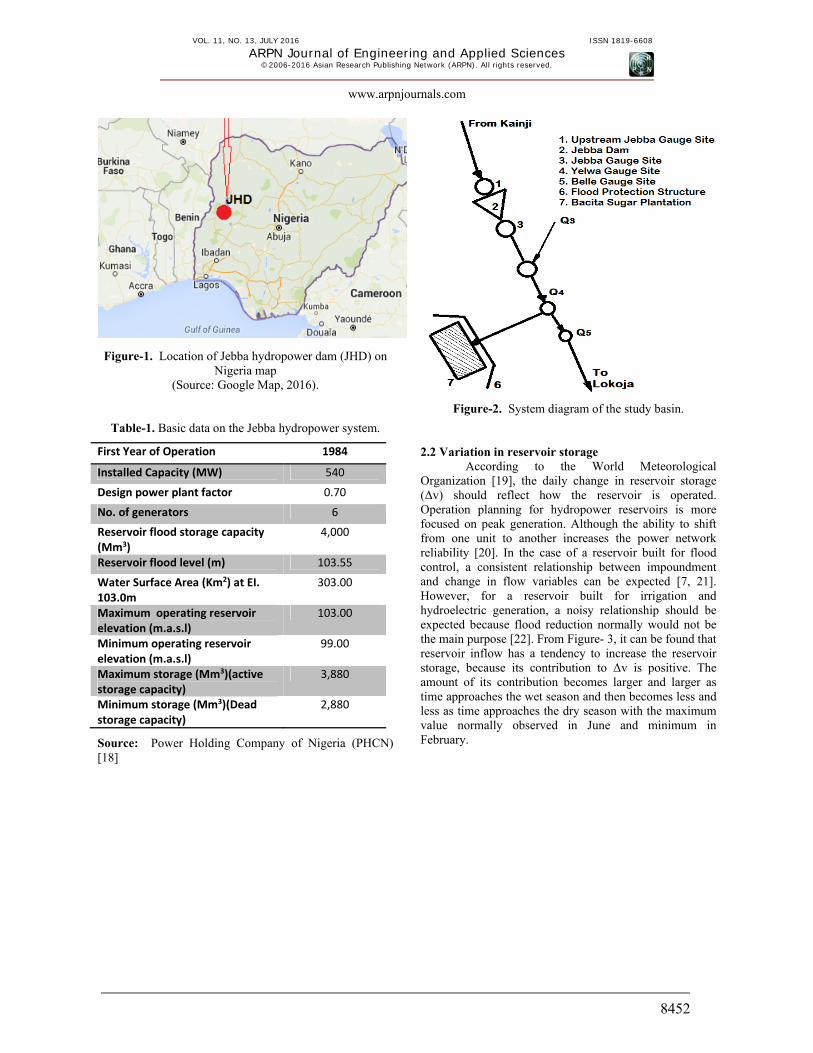
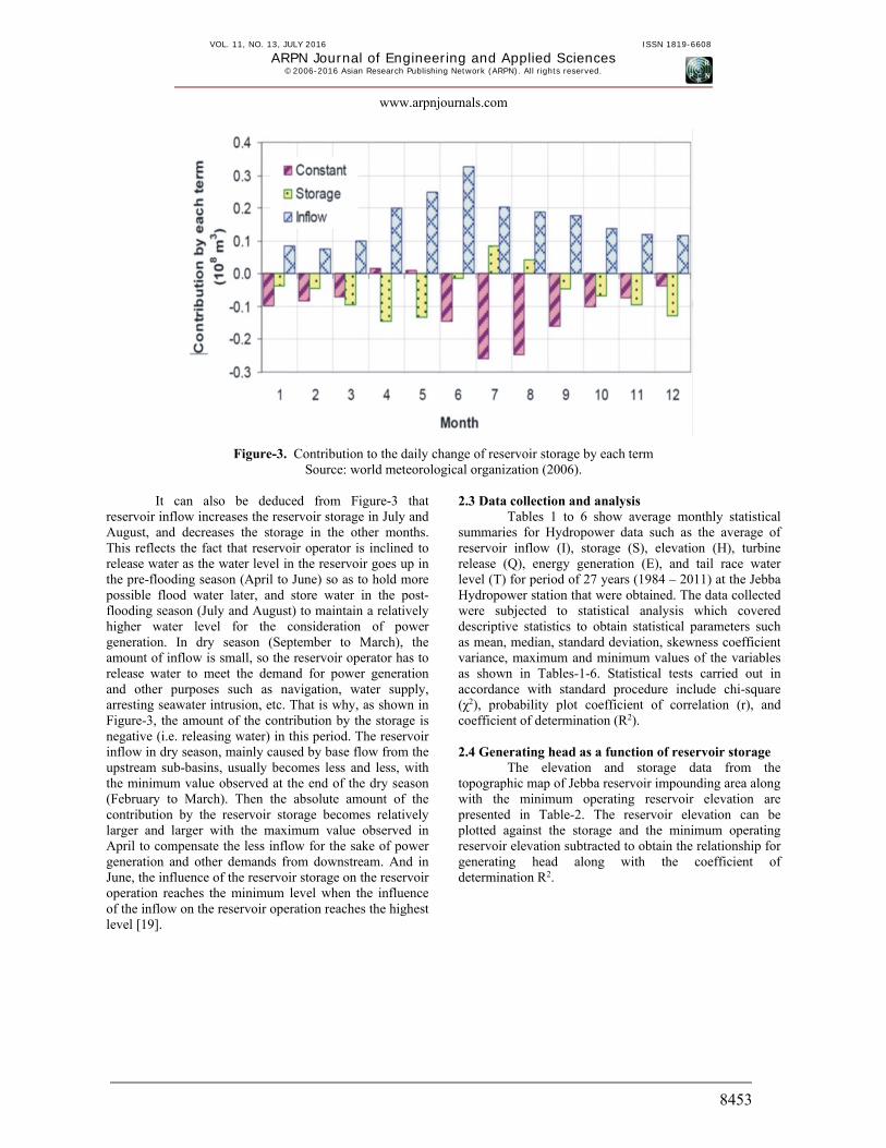
Jebba Hydroelectric Power Station is along River Niger, Nigeria, located between latitudes 9o 10’ N to 9o 55’ N and longitudes 4o 30’ E to 5o 00’ E at 76 m above sea level (about 100 kilometres downstream of Kainji dam). The station is one of the most cost-effective sources of electricity in Nigeria. It has maximum length of 100 kilometres (km), maximum depth of 32.5km, maximum width of 10 km and a mean depth of 3.3 m. The surface area is 350 km2, maximum volume of 1000 x 106 m3, operating head of 27.6 m and maximum flow per unit of 380 m3/s. The dam, which has a generating capacity of 540 MW from six (6) turbines of 95 MW of power each, is enough to power over 364, 000 homes at operating head of 27.6 m. Each turbine is coupled to a generator of 119 MVA maximum continuous rating and 103.50 MVA base load rating. The dam was developed and constructed in 1979 and there has been no overhaul of the dam since inception. However, the station has been able to carry out routine minor and major repair works, and preventive maintenance which has kept the station performance well above average. Figure-1 show the location of Jebba Hydropower Dam on the Nigeria map and Table-1 represents the basic data on Jebba Hydropower System. Figure-2 shows the System Diagram of the Study Basin.
VOL. 11, NO. 13, JULY 2016 ISSN 1819-6608
ARPN Journal of Engineering and Applied Sciences ©2006-2016 Asian Research Publishing Network (ARPN). All rights reserved.
www.arpnjournals.com
8452
Figure-1. Location of Jebba hydropower dam (JHD) on Nigeria map
(Source: Google Map, 2016).
Table-1. Basic data on the Jebba hydropower system.
First Year of Operation 1984
Installed Capacity (MW) 540
Design power plant factor 0.70
No. of generators 6
Reservoir flood storage capacity (Mm3)
4,000
Reservoir flood level (m) 103.55
Water Surface Area (Km2) at EI. 103.0m
303.00
Maximum operating reservoir elevation (m.a.s.l)
103.00
Minimum operating reservoir elevation (m.a.s.l)
99.00
Maximum storage (Mm3)(active storage capacity)
3,880
Minimum storage (Mm3)(Dead storage capacity)
2,880
Source: Power Holding Company of Nigeria (PHCN) [18]
Figure-2. System diagram of the study basin. 2.2 Variation in reservoir storage
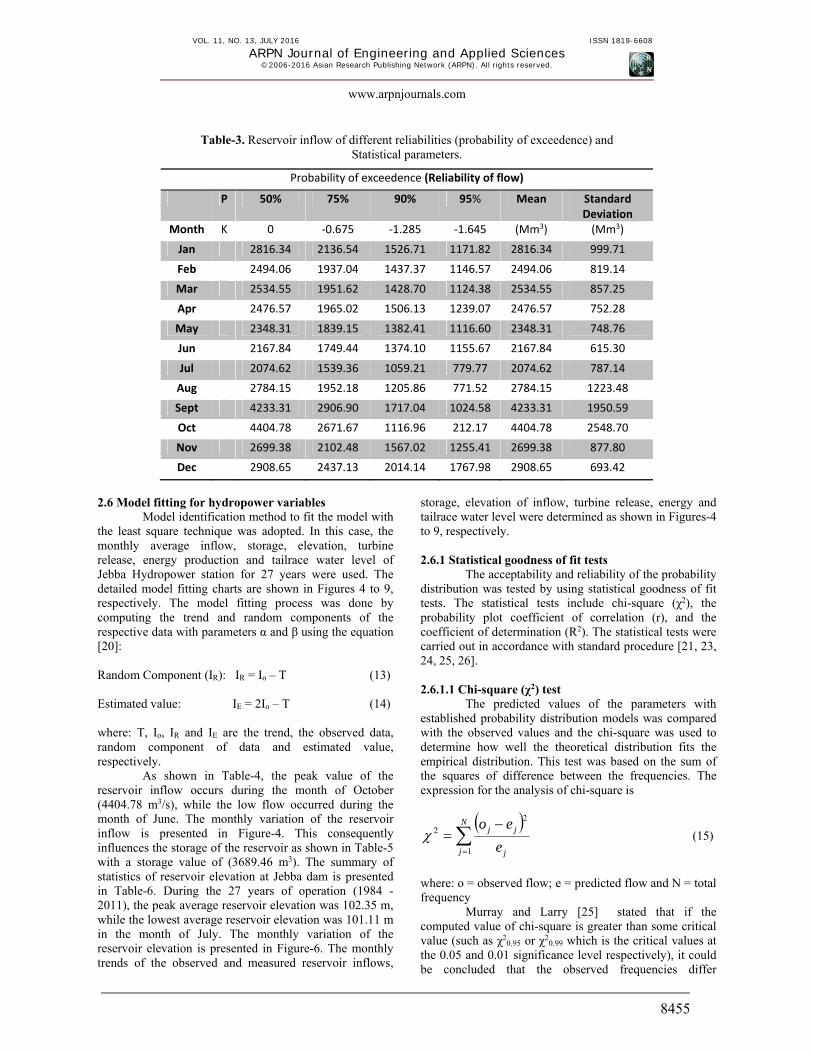
According to the World Meteorological Organization [19], the daily change in reservoir storage (Δv) should reflect how the reservoir is operated. Operation planning for hydropower reservoirs is more focused on peak generation. Although the ability to shift from one unit to another increases the power network reliability [20]. In the case of a reservoir built for flood control, a consistent relationship between impoundment and change in flow variables can be expected [7, 21]. However, for a reservoir built for irrigation and hydroelectric generation, a noisy relationship should be expected because flood reduction normally would not be the main purpose [22]. From Figure- 3, it can be found that reservoir inflow has a tendency to increase the reservoir storage, because its contribution to Δv is positive. The amount of its contribution becomes larger and larger as time approaches the wet season and then becomes less and less as time approaches the dry season with the maximum value normally observed in June and minimum in February.
VOL. 11, NO. 13, JULY 2016 ISSN 1819-6608
ARPN Journal of Engineering and Applied Sciences ©2006-2016 Asian Research Publishing Network (ARPN). All rights reserved.
www.arpnjournals.com
8453
Figure-3. Contribution to the daily change of reservoir storage by each term Source: world meteorological organization (2006).
It can also be deduced from Figure-3 that
reservoir inflow increases the reservoir storage in July and August, and decreases the storage in the other months. This reflects the fact that reservoir operator is inclined to release water as the water level in the reservoir goes up in the pre-flooding season (April to June) so as to hold more possible flood water later, and store water in the post-flooding season (July and August) to maintain a relatively higher water level for the consideration of power generation. In dry season (September to March), the amount of inflow is small, so the reservoir operator has to release water to meet the demand for power generation and other purposes such as navigation, water supply, arresting seawater intrusion, etc. That is why, as shown in Figure-3, the amount of the contribution by the storage is negative (i.e. releasing water) in this period. The reservoir inflow in dry season, mainly caused by base flow from the upstream sub-basins, usually becomes less and less, with the minimum value observed at the end of the dry season (February to March). Then the absolute amount of the contribution by the reservoir storage becomes relatively larger and larger with the maximum value observed in April to compensate the less inflow for the sake of power generation and other demands from downstream. And in June, the influence of the reservoir storage on the reservoir operation reaches the minimum level when the influence of the inflow on the reservoir operation reaches the highest level [19].
2.3 Data collection and analysis Tables 1 to 6 show average monthly statistical
summaries for Hydropower data such as the average of reservoir inflow (I), storage (S), elevation (H), turbine release (Q), energy generation (E), and tail race water level (T) for period of 27 years (1984 – 2011) at the Jebba Hydropower station that were obtained. The data collected were subjected to statistical analysis which covered descriptive statistics to obtain statistical parameters such as mean, median, standard deviation, skewness coefficient variance, maximum and minimum values of the variables as shown in Tables-1-6. Statistical tests carried out in accordance with standard procedure include chi-square (χ2), probability plot coefficient of correlation (r), and coefficient of determination (R2). 2.4 Generating head as a function of reservoir storage
The elevation and storage data from the topographic map of Jebba reservoir impounding area along with the minimum operating reservoir elevation are presented in Table-2. The reservoir elevation can be plotted against the storage and the minimum operating reservoir elevation subtracted to obtain the relationship for generating head along with the coefficient of determination R2.

VOL. 11, NO. 13, JULY 2016 ISSN 1819-6608
ARPN Journal of Engineering and Applied Sciences ©2006-2016 Asian Research Publishing Network (ARPN). All rights reserved.
www.arpnjournals.com
8454
Table-2. Reservoir elevation-storage data and the minimum operating reservoir elevation.
Reservoir elevation, Hr (m)
Reservoir capacityS (Mm3)
Minimum operating reservoir elevation,
Hmin2,t (m)
100.00 3050 99.00
100.25 3110 99.00
100.50 3180 99.00
100.75 3240 99.00
101.00 3300 99.00
101.25 3380 99.00
101.50 3460 99.00
101.75 3530 99.00
102.00 3600 99.00
102.25 3670 99.00
102.50 3730 99.00
102.75 3810 99.00
103.00 3880 99.00
Source: Technical report on Jebba Hydropower Station (2012) 2.5 Estimation of reservoir inflow of various Probabilities of exceedence
The reservoir inflow was fitted into normal distribution based on the monthly mean and standard deviation of the historical data. The normal models obtained for the month of January to December are presented in equations (1) to (12) respectively, the predicted reservoir inflow of 50%, 75%, 90%, and 95% probabilities of exceedence and statistical parameters are presented in Table-3.
KQJanuary 71.99934.2816 (1)
KQFebruary 14.81906.2494 (2)
KQMarch 25.85755.2534 (3)
KQApril 28.75257.2476 (4)
KQMay 76.74831.2348 (5)
KQJune 30.61584.2167 (6)
KQJuly 14.78762.2074 (7)
KQAugust 48.122315.2784 (8)
KQSeptember 59.195031.4233 (9)
KQOctober 70.254878.4404 (10)
KQNovember 80.87738.2699 (11)
KQDecember 42.69365.2908 (12)
VOL. 11, NO. 13, JULY 2016 ISSN 1819-6608
ARPN Journal of Engineering and Applied Sciences ©2006-2016 Asian Research Publishing Network (ARPN). All rights reserved.
www.arpnjournals.com
8455
Table-3. Reservoir inflow of different reliabilities (probability of exceedence) and
Statistical parameters.
Probability of exceedence (Reliability of flow)
P 50% 75% 90% 95% Mean Standard Deviation
Month K 0 ‐0.675 ‐1.285 ‐1.645 (Mm3) (Mm3)
Jan 2816.34 2136.54 1526.71 1171.82 2816.34 999.71
Feb 2494.06 1937.04 1437.37 1146.57 2494.06 819.14
Mar 2534.55 1951.62 1428.70 1124.38 2534.55 857.25
Apr 2476.57 1965.02 1506.13 1239.07 2476.57 752.28
May 2348.31 1839.15 1382.41 1116.60 2348.31 748.76
Jun 2167.84 1749.44 1374.10 1155.67 2167.84 615.30
Jul 2074.62 1539.36 1059.21 779.77 2074.62 787.14
Aug 2784.15 1952.18 1205.86 771.52 2784.15 1223.48
Sept 4233.31 2906.90 1717.04 1024.58 4233.31 1950.59
Oct 4404.78 2671.67 1116.96 212.17 4404.78 2548.70
Nov 2699.38 2102.48 1567.02 1255.41 2699.38 877.80
Dec 2908.65 2437.13 2014.14 1767.98 2908.65 693.42
2.6 Model fitting for hydropower variables
Model identification method to fit the model with the least square technique was adopted. In this case, the monthly average inflow, storage, elevation, turbine release, energy production and tailrace water level of Jebba Hydropower station for 27 years were used. The detailed model fitting charts are shown in Figures 4 to 9, respectively. The model fitting process was done by computing the trend and random components of the respective data with parameters α and β using the equation [20]: Random Component (IR): IR = Io – T (13) Estimated value: IE = 2Io – T (14) where: T, Io, IR and IE are the trend, the observed data, random component of data and estimated value, respectively.
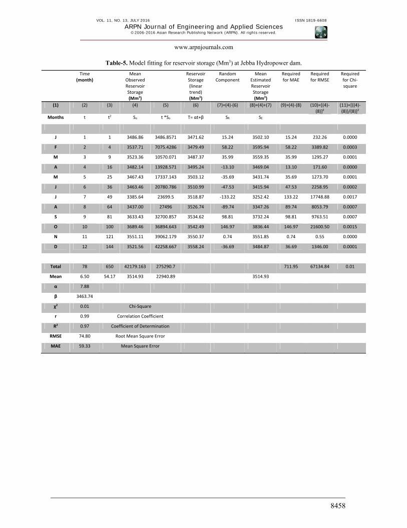
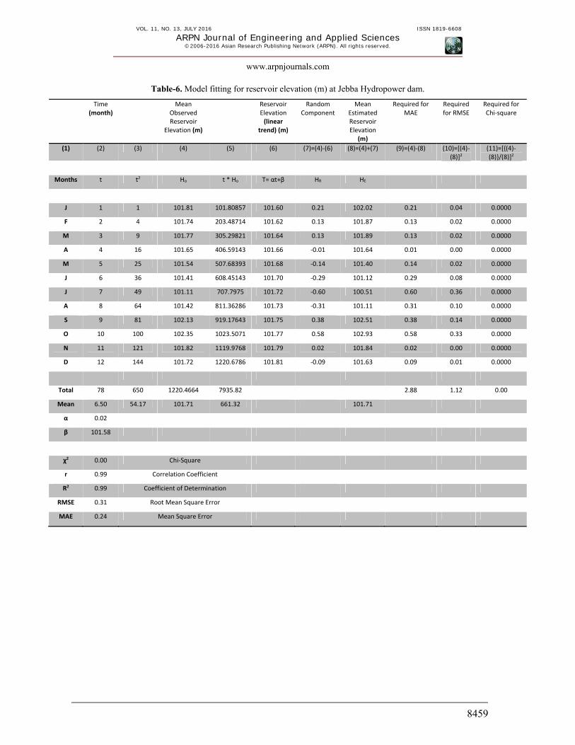
As shown in Table-4, the peak value of the reservoir inflow occurs during the month of October (4404.78 m3/s), while the low flow occurred during the month of June. The monthly variation of the reservoir inflow is presented in Figure-4. This consequently influences the storage of the reservoir as shown in Table-5 with a storage value of (3689.46 m3). The summary of statistics of reservoir elevation at Jebba dam is presented in Table-6. During the 27 years of operation (1984 - 2011), the peak average reservoir elevation was 102.35 m, while the lowest average reservoir elevation was 101.11 m in the month of July. The monthly variation of the reservoir elevation is presented in Figure-6. The monthly trends of the observed and measured reservoir inflows,
storage, elevation of inflow, turbine release, energy and tailrace water level were determined as shown in Figures-4 to 9, respectively.
2.6.1 Statistical goodness of fit tests
The acceptability and reliability of the probability distribution was tested by using statistical goodness of fit tests. The statistical tests include chi-square (χ2), the probability plot coefficient of correlation (r), and the coefficient of determination (R2). The statistical tests were carried out in accordance with standard procedure [21, 23, 24, 25, 26]. 2.6.1.1 Chi-square (χ2) test
The predicted values of the parameters with established probability distribution models was compared with the observed values and the chi-square was used to determine how well the theoretical distribution fits the empirical distribution. This test was based on the sum of the squares of difference between the frequencies. The expression for the analysis of chi-square is
N
j j
jj
e
eo
1
2
2 (15)
where: o = observed flow; e = predicted flow and N = total frequency
Murray and Larry [25] stated that if the computed value of chi-square is greater than some critical value (such as χ2
0.95 or χ20.99 which is the critical values at
the 0.05 and 0.01 significance level respectively), it could be concluded that the observed frequencies differ

VOL. 11, NO. 13, JULY 2016 ISSN 1819-6608
ARPN Journal of Engineering and Applied Sciences ©2006-2016 Asian Research Publishing Network (ARPN). All rights reserved.
www.arpnjournals.com
8456
significantly from the expected frequencies and it would be rejected, otherwise it would be accepted. Hence, if the χ2 value calculated from equation (15) is less than critical value from statistical table, the model can be concluded to be strong or the fit of the data is good. Another way by which the conclusion can be made is that if the value of the ratio of calculated chi-square to the tabulated chi-square (χ2
cal / χ2tab) is less than one, the probability
distribution is strong. The distribution function that gives value very close to 1 is the best for the data [25]. 2.6.1.2 Probability plot correlation coefficient (PPCC)
This is used to evaluate the linearity of the probability plot, so that if the sample is actively drawn from the hypothesized distribution the PPCC (r) is expected to be close to one. The quantity (r) called coefficient of correlation is given as:
2
2
meanobs
meanest
QQr
(16)
Where: Qest = the value of inflow estimated with the
probability function Qmean = the mean value of the observed inflow and Qobs = the value of the observed Inflow 2.6.1.3 Coefficient of determination (R2)
This is a measure of the strength of relationship between the predictor and response variables. According to [27], the coefficient of determination in the regression theory is defined as:
o
o
E
EER
2 (17)
Where:
N
imeaniobsio QQE
1
2)()( (18)
N
iestiobsi QQE 2
)()( (19)
Qi(est) is the model output in the ith time period, Qi
(obs) is the observed data in the same period and Qi(mean) is the mean over the observed periods. The model is strong, if R2 is very close to one. 2.6.1.4 Error of estimate
Two errors of estimate were taken into consideration for comparison of results in accordance to [28]. The first of them is the Root Mean Square Error (RMSE), which is given as:
n
ipredobs iQiQnRMSE
1
21 )()( (20)
The second is the Mean Absolute Error (MAE), which is defined as
n
ipredobs iQiQnMAE
1
1 )()( (21)

VOL. 11, NO. 13, JULY 2016 ISSN 1819-6608
ARPN Journal of Engineering and Applied Sciences ©2006-2016 Asian Research Publishing Network (ARPN). All rights reserved.
www.arpnjournals.com
8457
Table-4. Model fitting for reservoir inflow (Mm3) at Jebba hydropower dam.
Time (month)
Mean Observed Reservoir Inflow (Mm3)
Reservoir Inflow (linear trend) (Mm3)
Random Component
Mean Estimated Reservoir Inflow (Mm3)
Required for MAE
Required for RMSE
Required for Chi‐square
(1) (2) (3) (4) (5) (6) (7)=(4)‐(6) (8)=(4)+(7)
(9)=(4)‐(8)
(10)= [(4)‐(8)]2
(11)=[{(4)‐(8)}/(8)]2
Months t t2 Io t * Io T= αt+β IR IE
J 1 1 2816.34 2816.3394 2329.45 486.89 3303.23 486.89 237059.30 0.0217
F 2 4 2494.06 4988.117 2420.20 73.86 2567.92 73.86 5455.61 0.0008
M 3 9 2534.55 7603.6596 2510.94 23.61 2558.17 23.61 557.54 0.0001
A 4 16 2476.57 9906.2723 2601.69 ‐125.12 2351.45 125.12 15654.32 0.0028
M 5 25 2348.31 11741.556 2692.43 ‐344.12 2004.19 344.12 118417.58 0.0295
J 6 36 2167.84 13007.054 2783.17 ‐615.33 1552.51 615.33 378633.27 0.1571
J 7 49 2074.62 14522.309 2873.92 ‐799.30 1275.31 799.30 638885.25 0.3928
A 8 64 2784.15 22273.181 2964.66 ‐180.52 2603.63 180.52 32585.81 0.0048
S 9 81 4233.31 38099.75 3055.41 1177.90 5411.20 1177.90 1387443.93 0.0474
O 10 100 4404.78 44047.836 3146.15 1258.63 5663.42 1258.63 1584153.83 0.0494
N 11 121 2699.38 29693.188 3236.90 ‐537.52 2161.87 537.52 288922.95 0.0618
D 12 144 2908.65 34903.807 3327.64 ‐418.99 2489.66 418.99 175552.70 0.0283
Total 78 650 33942.556 233603.07 6041.78 4863322.10 0.80
Mean 6.50 54.17 2828.55 19466.92 2828.55
α 90.74
β 2238.71
χ2 0.80 Chi‐Square
R 0.98 Correlation Coefficient
R2 0.95 Coefficient of Determination
RMSE 636.61 Root Mean Square Error
MAE 503.48 Mean Square Error
VOL. 11, NO. 13, JULY 2016 ISSN 1819-6608
ARPN Journal of Engineering and Applied Sciences ©2006-2016 Asian Research Publishing Network (ARPN). All rights reserved.
www.arpnjournals.com
8458
Table-5. Model fitting for reservoir storage (Mm3) at Jebba Hydropower dam.
Time (month)
Mean Observed Reservoir Storage (Mm3)
Reservoir Storage (linear trend) (Mm3)
Random Component
Mean Estimated Reservoir Storage (Mm3)
Required for MAE
Required for RMSE
Required for Chi‐square
(1) (2) (3) (4) (5) (6) (7)=(4)‐(6) (8)=(4)+(7) (9)=(4)‐(8) (10)=[(4)‐(8)]2
(11)=[{(4)‐(8)}/(8)]2
Months t t2 So t *So T= αt+β SR SE
J 1 1 3486.86 3486.8571 3471.62 15.24 3502.10 15.24 232.26 0.0000
F 2 4 3537.71 7075.4286 3479.49 58.22 3595.94 58.22 3389.82 0.0003
M 3 9 3523.36 10570.071 3487.37 35.99 3559.35 35.99 1295.27 0.0001
A 4 16 3482.14 13928.571 3495.24 ‐13.10 3469.04 13.10 171.60 0.0000
M 5 25 3467.43 17337.143 3503.12 ‐35.69 3431.74 35.69 1273.70 0.0001
J 6 36 3463.46 20780.786 3510.99 ‐47.53 3415.94 47.53 2258.95 0.0002
J 7 49 3385.64 23699.5 3518.87 ‐133.22 3252.42 133.22 17748.88 0.0017
A 8 64 3437.00 27496 3526.74 ‐89.74 3347.26 89.74 8053.79 0.0007
S 9 81 3633.43 32700.857 3534.62 98.81 3732.24 98.81 9763.51 0.0007
O 10 100 3689.46 36894.643 3542.49 146.97 3836.44 146.97 21600.50 0.0015
N 11 121 3551.11 39062.179 3550.37 0.74 3551.85 0.74 0.55 0.0000
D 12 144 3521.56 42258.667 3558.24 ‐36.69 3484.87 36.69 1346.00 0.0001
Total 78 650 42179.163 275290.7 711.95 67134.84 0.01
Mean 6.50 54.17 3514.93 22940.89 3514.93
α 7.88
β 3463.74
χ2 0.01 Chi‐Square
r 0.99 Correlation Coefficient
R2 0.97 Coefficient of Determination
RMSE 74.80 Root Mean Square Error
MAE 59.33 Mean Square Error
VOL. 11, NO. 13, JULY 2016 ISSN 1819-6608
ARPN Journal of Engineering and Applied Sciences ©2006-2016 Asian Research Publishing Network (ARPN). All rights reserved.
www.arpnjournals.com
8459
Table-6. Model fitting for reservoir elevation (m) at Jebba Hydropower dam.
Time (month)
Mean Observed Reservoir
Elevation (m)
Reservoir Elevation (linear
trend) (m)
Random Component
Mean Estimated Reservoir Elevation
(m)
Required for MAE
Required for RMSE
Required for Chi‐square
(1) (2) (3) (4) (5) (6) (7)=(4)‐(6) (8)=(4)+(7) (9)=(4)‐(8) (10)=[(4)‐(8)]2
(11)=[{(4)‐(8)}/(8)]2
Months t t2 Ho t * Ho T= αt+β HR HE
J 1 1 101.81 101.80857 101.60 0.21 102.02 0.21 0.04 0.0000
F 2 4 101.74 203.48714 101.62 0.13 101.87 0.13 0.02 0.0000
M 3 9 101.77 305.29821 101.64 0.13 101.89 0.13 0.02 0.0000
A 4 16 101.65 406.59143 101.66 ‐0.01 101.64 0.01 0.00 0.0000
M 5 25 101.54 507.68393 101.68 ‐0.14 101.40 0.14 0.02 0.0000
J 6 36 101.41 608.45143 101.70 ‐0.29 101.12 0.29 0.08 0.0000
J 7 49 101.11 707.7975 101.72 ‐0.60 100.51 0.60 0.36 0.0000
A 8 64 101.42 811.36286 101.73 ‐0.31 101.11 0.31 0.10 0.0000
S 9 81 102.13 919.17643 101.75 0.38 102.51 0.38 0.14 0.0000
O 10 100 102.35 1023.5071 101.77 0.58 102.93 0.58 0.33 0.0000
N 11 121 101.82 1119.9768 101.79 0.02 101.84 0.02 0.00 0.0000
D 12 144 101.72 1220.6786 101.81 ‐0.09 101.63 0.09 0.01 0.0000
Total 78 650 1220.4664 7935.82 2.88 1.12 0.00
Mean 6.50 54.17 101.71 661.32 101.71
α 0.02
β 101.58
χ2 0.00 Chi‐Square
r 0.99 Correlation Coefficient
R2 0.99 Coefficient of Determination
RMSE 0.31 Root Mean Square Error
MAE 0.24 Mean Square Error

VOL. 11, NO. 13, JULY 2016 ISSN 1819-6608
ARPN Journal of Engineering and Applied Sciences ©2006-2016 Asian Research Publishing Network (ARPN). All rights reserved.
www.arpnjournals.com
8460
Table-7. Model fitting for turbine release (Mm3) at Jebba Hydropower dam.
Time (month)
Mean Observed Turbine Release (Mm3)
Reservoir Inflow (linear trend) (Mm3)
Random Component
Mean Estimated Turbine Release (Mm3)
Required for MAE
Required for RMSE
Required for Chi‐square
(1) (2) (3) (4) (5) (6) (7)=(4)‐(6) (8)=(4)+(7) (9)=(4)‐(8)
(10)=[(4)‐(8)]2
(11)=[{(4)‐(8)}/(8)]2
Months t t2 Qo t *Qo T= αt+β QR QE
J 1 1 2923.58 2923.5841 2481.73 441.86 3365.44 441.86 195236.22 0.0172
F 2 4 2604.83 5209.6613 2517.79 87.04 2691.87 87.04 7576.30 0.0010
M 3 9 2527.23 7581.6921 2553.85 ‐26.62 2500.61 26.62 708.52 0.0001
A 4 16 2529.42 10117.675 2589.91 ‐60.49 2468.93 60.49 3659.03 0.0006
M 5 25 2338.30 11691.517 2625.97 ‐287.67 2050.64 287.67 82751.34 0.0197
J 6 36 2212.31 13273.875 2662.03 ‐449.72 1762.60 449.72 202244.60 0.0651
J 7 49 2083.62 14585.359 2698.09 ‐614.47 1469.16 614.47 377568.40 0.1749
A 8 64 2772.19 22177.498 2734.15 38.04 2810.23 38.04 1446.94 0.0002
S 9 81 3199.80 28798.216 2770.21 429.59 3629.39 429.59 184550.32 0.0140
O 10 100 3558.63 35586.267 2806.27 752.36 4310.98 752.36 566042.76 0.0305
N 11 121 2673.61 29409.755 2842.33 ‐168.71 2504.90 168.71 28464.57 0.0045
D 12 144 2737.17 32846.051 2878.39 ‐141.22 2595.95 141.22 19942.41 0.0030
Total 78 650 32160.704 214201.15 3497.77 1670191.41 0.33
Mean 6.50 54.17 2680.06 17850.10 2580.06
α 36.06
β 2445.67
χ2 0.33 Chi‐Square
r 0.99 Correlation Coefficient
R2 0.98 Coefficient of Determination
RMSE 373.07 Root Mean Square Error
MAE 291.48 Mean Square Error

VOL. 11, NO. 13, JULY 2016 ISSN 1819-6608
ARPN Journal of Engineering and Applied Sciences ©2006-2016 Asian Research Publishing Network (ARPN). All rights reserved.
www.arpnjournals.com
8461
Table-8. Model fitting for energy generation (Mwh) at Jebba Hydropower dam.
Time (month) Mean Observed Energy (Mwh)
Energy Generation (linear trend) (Mwh)
Random Component
Mean Estimated Turbine Release (Mwh)
Required for MAE
Required for RMSE
Required for Chi‐square
(1) (2) (3) (4) (5) (6) (7)=(4)‐(6) (8)=(4)+(7) (9)=(4)‐(8) (10)=[(4)‐(8)]2 (11)=[{(4)‐(8)}/(8)]2
Months t t2 Eo t *Eo T= αt+β ER EE
J 1 1 201149.2 201149.15 174010.16 27138.99 228288.14 27138.99 736524518.76 0.0141
F 2 4 179092.5 358185.09 176190.17 2902.37 181994.92 2902.37 8423769.62 0.0003
M 3 9 183426.2 550278.71 178370.18 5056.05 188482.29 5056.05 25563669.61 0.0007
A 4 16 174818.9 699275.46 180550.19 ‐5731.33 169087.54 5731.33 32848123.82 0.0011
M 5 25 167722.0 838609.99 182730.20 ‐15008.20 152713.79 15008.20 225246175.57 0.0097
J 6 36 155854.9 935129.49 184910.21 ‐29055.30 126799.62 29055.30 844210272.03 0.0525
J 7 49 150044.0 1050308.2 187090.22 ‐37046.19 112997.85 37046.19 1372419848.59 0.1075
A 8 64 179755.6 1438044.7 189270.23 ‐9514.65 170240.94 9514.65 90528475.56 0.0031
S 9 81 223874.2 2014867.4 191450.24 32423.92 256298.07 32423.92 1051310430.10 0.0160
O 10 100 235006.1 2350061.4 193630.25 41375.89 276382.03 41375.89 1711964457.85 0.0224
N 11 121 191259.0 2103849.2 195810.26 ‐4551.24 186707.78 4551.24 20713787.77 0.0006
D 12 144 189999.9 2279999.3 197990.27 ‐7990.32 182009.62 7990.32 63845234.34 0.0019
Total 78 650 2232002.6 14819758 217794.44 6183598763.60 0.23
Mean 6.50 54.17 186000.22 1234979.85 186000.22
α 2180.01
β 171830.16
χ2 0.23 Chi‐Square
r 0.99 Correlation Coefficient
R2 0.98 Coefficient of Determination
RMSE 22700.22 Root Mean Square Error
MAE 18149.54 Mean Square Error

VOL. 11, NO. 13, JULY 2016 ISSN 1819-6608
ARPN Journal of Engineering and Applied Sciences ©2006-2016 Asian Research Publishing Network (ARPN). All rights reserved.
www.arpnjournals.com
8462
Table-9. Model fitting for tailrace water level (m) at Jebba Hydropower dam.
Time (month)
Mean Observed Tailrace Water
Level (m)
Tailrace Water level (linear trend) (m)
Random Component
Mean Estimated Tailrace
water level (m)
Required for MAE
Required for RMSE
Required for Chi‐square
(1) (2) (3) (4) (5) (6) (7)=(4)‐(6) (8)=(4)+(7) (9)=(4)‐(8) (10)=[(4)‐(8)]2
(11)=[{(4)‐(8)}/(8)]2
Months t t2 To t *To T= αt+β TR TE
J 1 1 73.92 73.920714 73.57 0.35 74.27 0.35 0.12 0.000022
F 2 4 73.77 147.54214 73.60 0.17 73.94 0.17 0.03 0.000005
M 3 9 73.67 221.01964 73.64 0.03 73.71 0.03 0.00 0.000000
A 4 16 73.58 294.32 73.67 ‐0.09 73.49 0.09 0.01 0.000002
M 5 25 73.43 367.12857 73.71 ‐0.28 73.14 0.28 0.08 0.000015
J 6 36 73.33 439.99071 73.74 ‐0.41 72.92 0.41 0.17 0.000032
J 7 49 73.22 512.5725 73.78 ‐0.55 72.67 0.55 0.31 0.000058
A 8 64 73.63 589.00286 73.81 ‐0.19 73.44 0.19 0.03 0.000006
S 9 81 74.37 669.3075 73.85 0.52 74.89 0.52 0.27 0.000048
O 10 100 74.58 745.75714 73.88 0.70 75.27 0.70 0.48 0.000085
N 11 121 73.84 812.185 73.92 ‐0.08 73.75 0.08 0.01 0.000001
D 12 144 73.79 885.45857 73.95 ‐0.16 73.63 0.16 0.03 0.000005
Total 78 650 885.11893 5758.2054 3.53 1.54 0.000280
Mean 6.50 54.17 73.76 479.85 73.76
α 0.03
β 73.54
χ2 0.00028 Chi‐Square
r 0.99 Correlation Coefficient
R2 0.98 Coefficient of Determination
RMSE 0.36 Root Mean Square Error
MAE 0.29 Mean Square Error

VOL. 11, NO. 13, JULY 2016 ISSN 1819-6608
ARPN Journal of Engineering and Applied Sciences ©2006-2016 Asian Research Publishing Network (ARPN). All rights reserved.
www.arpnjournals.com
8463
Figure-4. Model fitting for reservoir inflow of Jebba hydropower dam.
Figure-5. Model fitting for reservoir storage of Jebba hydropower dam.
Figure-6. Model fitting for reservoir elevation of Jebba hydropower dam.

VOL. 11, NO. 13, JULY 2016 ISSN 1819-6608
ARPN Journal of Engineering and Applied Sciences ©2006-2016 Asian Research Publishing Network (ARPN). All rights reserved.
www.arpnjournals.com
8464
Figure-7. Model fitting for turbine release of Jebba hydropower dam.
Figure-8. Model fitting for energy generation of Jebba hydropower dam.
Figure-9. Model fitting for tailrace water level of Jebba hydropower dam.

VOL. 11, NO. 13, JULY 2016 ISSN 1819-6608
ARPN Journal of Engineering and Applied Sciences ©2006-2016 Asian Research Publishing Network (ARPN). All rights reserved.
www.arpnjournals.com
8465
Table-10 shows the excess water release, evaporation loss and rainfall at Jebba Hydropower Dam. The mean and the maximum spillage is recorded in the month of October with attendant highest evaporation loss.
From January to July, there is no spillage unlike August through to December.
Table-10. Excess water release, evaporation loss and rainfall at Jebba H.P dam.
Spillage at Jebba H.P dam (1984 - 2006) Evaporation loss / Rainfall at Jebba H.P dam (1984 - 2006)
Month Mean spillage
( tG ,2 )
Max. spillage
( tG ,2ˆ )
Evaporation loss Rainfall
Mm3 Mm3 Mm Mm3 Mm Mm3
Jan 0.00 0.00 177.1 53.66 0.07 0.02
Feb 0.00 0.00 244.0 73.93 1.85 0.56
Mar 0.00 0.00 241.0 73.03 14.63 4.44
Apr 0.00 0.00 269.6 81.69 68.84 20.86
May 0.00 0.00 209.3 63.42 148.13 44.89
Jun 0.00 0.00 176.0 53.33 211.09 63.96
Jul 0.00 0.00 143.0 43.33 168.95 51.20
Aug 94.52 507.99 123.4 37.39 188.82 57.22
Sept 624.05 2230.93 139.2 42.18 221.62 67.15
Oct 792.73 2691.21 193.4 58.60 80.59 24.42
Nov 118.85 607.91 200.5 60.75 0.71 0.22
Dec 187.25 868.20 186.7 56.57 0.00 0.00
Evaporation loss (Mm3) = Evaporation depth × Lake surface area =303 km2. Direct Rainfall inflow (Mm3) = Rainfall depth × Lake surface area
3. RESULTS AND DISCUSSIONS
Tables 4 to 9 show average monthly statistical summaries for reservoir inflow, storage, elevation, turbine release, energy generated and tailrace water level, respectively, for periods of 1984 - 2011. The least square technique was adopted to fit the model which resulted into equations (13) and (14). The fitted models results computations and the resulting charts for the predicted data and the statistical goodness of fit tests (such as the chi-square, correlation coefficient, root mean square error, coefficient of determination and the mean square error), are shown in Tables 4 to 9 and Figures-4 to 9, respectively. As shown in Tables 4-9, the spread of the computed data are scattered and non-uniform throughout the year. The high spread of inflow, storage, energy generation and turbine release is a significant pointer that the hydrological process is not being uniform throughout the years. It is also clear that the four parameters (inflow, storage, energy generation and turbine release) are closely related. The pattern is similar with higher values in September-October and lower values in June-July. This seasonal routine is identified as an important factor influencing the functioning of the reservoir servicing the Hydropower dam. It was observed that the mean expectations on both the observed and estimated parameter values are the same for all parameters of inflow, storage,
elevation, turbine release, energy generation and the tailrace water level.
For the reservoir inflow, there appears to be large errors of the RMSE and MAE but with reasonable results for the chi-square, correlation coefficient and coefficient of determination. The same was identified for reservoir storage, turbine release and energy generation. These also correspond to the fact that their parameters were scattered. The model fitting charts for all the parameters (Figures 4- 9) show that, the predicted values begun slightly above the observed values and ends slightly below the observed values. In the probability of exceedence (reliability of flow) computed using normal distribution (Table-3), the values are in descending orders in the order of 50%, 75%, 90% and 95%. The optimal solution obtained at operation performance of 50% reservoir inflow reliability has the total annual energy generation of 42105.63MWH. The average optimal energy generation obtained is 19% of the observed energy generation but with adequate water supply for downstream users and for irrigation throughout the year. 4. CONCLUSIONS
The paper captures important issues that must be taken into account and the potential benefits that can be realized when appropriate measures are taken into consideration in the management of reservoir for

VOL. 11, NO. 13, JULY 2016 ISSN 1819-6608
ARPN Journal of Engineering and Applied Sciences ©2006-2016 Asian Research Publishing Network (ARPN). All rights reserved.
www.arpnjournals.com
8466
hydropower and flood management purposes. Flood occurrence in the downstream regime is caused majorly by the sudden release of water from the hydropower dams located upstream of the study area. The determination of the amount of reservoir for a specified purpose such as flood control is based on hydrologic analyses that are governed by project formulation criteria. Previous literature has established that it is necessary to define specific rules that will help distribute the available water resources because most reservoir systems exhibit a competition among water uses. The guiding formulation principles in most free enterprise countries are generally that the project, with the specified amount of storage, must be economically justified (benefit/cost ratio must exceed one), the project should be formulated in practical extent to maximize net economic benefits, and the project should not result in significantly increased flood hazards for any flood event, especially one that would exceed the design capacity of the reservoir system. Projects with conservation storage should also provide a reasonable guarantee (probability) of dependable water supply from the reservoirs.
The study revealed that the sudden release of flood water at Jebba is not due to normal operation at the hydropower station, but due to sudden discharges at the reservoirs located upstream in order to create enough space for the incoming flood water. This automatically forces the release of water at Jebba and thus creating flood problem downstream. The flow regime of the River Niger downstream of Jebba dam is governed by the operations of the Kanji and Jebba hydroelectric power schemes and runoff from the catchments. Releases from Kainji HEP dam constitute the major inflow into Jebba HEP dam since it lies directly under it. This mean that the more the releases from upper reservoir the faster the downstream reservoir fill up and excess will be discharged thereby leading to flooding. In addition, the annual discharge of rivers limits the overall energy output from hydropower plants. However, discharge records are relatively short and subject to fluctuations over different periods that may persist for many years. It is important that water planners and managers consider a number of allocation alternatives by using system models. This will help to define the proper criteria and procedures to balance the allocation rules. REFERENCES [1] J. O. Aribisala and B. F. Sule. 1998. Seasonal
operation of a Reservoir Hydropower system, Technical Transactions, Nigerian Society of Engineers, NSE. 33(2): 1-14.
[2] D. O. Olukanni and A. W. Salami. 2012. Assessment of Impact of Hydropower Dams Reservoir Outflow on the Downstream River Flood Regime - Nigeria’s Experience. Hydropower-Practice and Application.
[3] H. Samadi-Boroujen. 2012. Hydropower practice and application, Intech, Croatia
[4] J. L. B. Brandao. 2012 Reservoir Operation Applied to Hydropower Systems. Hydropower practice and application, InTech, Croatia. pp. 185-200.
[5] H. Locher and A. Scanlon. 2012. Sustainable hydropower- Issues and approaches, Hydropower practice and application, InTech, Croatia. pp. 1-22.
[6] P. Gourbesville. 2008. Challenges for Integrated Water Resources Management. J. Phys and Chem. of the Earth. 33: 284-289.
[7] R. J. Batalla, C. M. Gomez and G. M. Kondolf. 2004. Reservoir-induced hydrological changes in the Ebro River basin (NE Spain), Journal of Hydrology. 290(1-2): 117-136.
[8] A. Worman. 2012. Hydrological Statistics for Regulating Hydropower, Hydropower practice and application, InTech, Croatia. pp. 41-60.
[9] B. D. Ritcher, J. V. Baumgartner, J. Powell and D.P. Braun. 1996. A method for assessing hydrologic alteration within ecosystem, Conservative Biology, 10: 1163-1174.
[10] F. Lajoie, A. A. Assani, G. R. Andre and M. Mesfioui. 2007. Impacts of dams on monthlyflow characteristics. The influence of watershed size and seasons, Journal of Hydrology. 334, 423-439.
[11] N. Hanasaki, S. Kanae and T. Oki. 2006. A reservoir operation scheme for global river routing models, Journal of Hydrology. 327: 22-41.
[12] B. L. Maheshwari, K. F. Walker and T.A. McMahon. 1995. Effects of regulation on the flow regime of the River Murray, Australia, Regulated Rivers: Research and Management. 10: 15-38.
[13] H. S. Fahmy, J. P. King, M. W. Wentzel and J. A. Seton. 1994. Economic Optimization of River Management Using Genetic Algorithms. American Society Of Agricultural Engineers, St. Joseph, Mich. Paper no.943034, ASCE 1994 Int. Summer Meeting.
[14] M. G. Nogueria, P. C. Reis-Oliveira and Y. T. Britto. 2008. Zooplankton assemblages (Copepoda and Cladocera) in a cascade of reservoirs of a large tropical river (SE Brazil) Limmetica. 27: 151-170.

VOL. 11, NO. 13, JULY 2016 ISSN 1819-6608
ARPN Journal of Engineering and Applied Sciences ©2006-2016 Asian Research Publishing Network (ARPN). All rights reserved.
www.arpnjournals.com
8467
[15] T. G. Bosona and G. Gebresenbet. 2010. Modelling Hydropower Plant System to Improve its Reservoir Operation, International Journal of Water Resources and Environmental Engineering. 2(4): 87-94
[16] D. J. Obadote. 2009. Energy Crisis in Nigeria: Technical Issues and Solutions, Power Sector Conference, June 25v- 27.
[17] A. Worman, G. Lindstron, J. Riml and A. Akesson. 2010. Drifting runoff periodicity during the 30th century due to changing surface water volume, Hydrological Processes. 24(26): 3772- 3784.
[18] Jebba hydro-electric Power Station. 2010. Hydrology, Meteorology and Reservoir operational data. Hydrology section. Jebba, Niger State, Nigeria.
[19] World Meteorological Organization. 2006. Environmental Aspects of Integrated flood Management, APFM Technical Document No.3, Flood Management Policy Series (Geneva: Associated Programme on Flood Management). http://www.apfm.info/pdf/ifm_environmental_aspects.pdf. Accessed November 26, 2015.
[20] B. Zahraie and M. Karamouz. 2004. Hydropower Reservoirs Operation: A Time Decomposition Approach, Scientia Iranica. 11(1&2): 92-103.
[21] D. O. Olukanni and A. W. Salami. 2008. Fitting probability distribution functions to Reservoir inflow at hydropower dams in Nigeria. Journal of Environmental Hydrology. 16 (35): 1-7.
[22] K. F. Walker. 1985. A review of the ecological effects of river regulation in Australia, Hydrbiologia, 125: 111-129.
[23] J. U. Chowdhury and J. R. Stedinger. 1991. Goodness of fit tests for regional generalized extreme value Flood distributions. Water Resour. Res. 27(7): 1765-1776.
[24] O. S. Adegboye and R. A. Ipinyomi. 1995. Statistical tables for class work and examination. Tertiary publications Nigeria Limited, Ilorin, Nigeria. pp. 5-11.
[25] R. S. Murray and J. S. Larry. 2000. Theory and problems of statistics. Tata Mc Graw - Hill Publishing Company Limited, New Delhi. pp. 314-316, Third edition.
[26] D. O. Olukanni and M. O. Alatise. 2008. Rainfall-Runoff Relationships and Flow Forecasting, Ogun River, Nigeria. Journal of Environmental Hydrology. 16(23).
[27] B. Y. Dibike and D. P. Solomatine 1999. River flow forecasting using Artificial Neural Networks. Paper Presented at European Geophysical Society (EGS) xxiv General Assembly. The Hague, the Netherlands. 1-11.
[28] V. Z. Antonopoulos, D. M. Papamichail, and K. A. Mitsiou. 2001. Statistical and trend analysis of water quality and quantity data for the Strymon River in Greece. Hydrology and Earth Sciences. 5(4): 679-692.


