Assessment of Information and Communication Technologies:

Land Use and Congestion Management Strategies to Promote Urban Environmental Sustainability

Chris Hendrickson, Principal Investigator

Yeganeh Mashayekh, Research Assistant

Technologies for Safe and Efficient

University Transportation Center

Carnegie Mellon University

Pittsburgh, Pennsylvania

December, 2013

ii

DISCLAIMER

The contents of this report reflect the views of the authors, who are responsible for the facts and the

accuracy of the information presented herein. This document is disseminated under the sponsorship of the

U.S. Department of Transportation’s University Transportation Centers Program, in the interest of

information exchange. The U.S. Government assumes no liability for the contents or use thereof.

iii

Abstract

Reducing greenhouse gas emissions (GHG) is an important social goal to mitigate

climate change. A common mitigation paradigm is to consider strategy ‘wedges’ that

can be applied to different activities to achieve desired GHG reductions. In this report,

we consider a wide range of possible travel demand reduction and traffic congestion

management strategies to reduce light-duty vehicle GHG emissions.

To estimate the cost savings associated with the implementation of various travel

demand and traffic congestion management strategies, performance measures such as

speed, delay, and travel time were assessed for each strategy. These performance

measures were then combined with emission factors – amount of pollutants per speed

interval – and monetary damage values of each pollutant in terms of mortality,

morbidity and environmental damages – dollar per gram of pollutant – to estimate the

external environmental cost savings resulting from the implemented strategy. Fuel and

time cost savings were simply measured by incorporating the value of time and fuel.

Specifically, the external environmental cost of driving in the U.S. including

congestion was estimated to be about $110 billion annually. Brownfield developments

and LEED certified brownfield developments were assessed as land use and travel

demand management strategies to reduce vehicular travel demand. Impacts of these

residential developments on vehicle miles traveled (VMT) reduction and the resulting

costs (cost of driving time, fuel, and external air pollution costs) were examined. Results

show with minimal implementation cost incurred by transportation authorities (about

75-95% less than other VMT reduction measures), both brownfield residential

developments and LEED certified brownfield residential developments can be

beneficial travel demand strategies, assisting federal, state and local governments with

their GHG emissions reduction goals. Compared with conventional developments,

residential brownfield developments can reduce VMT and its consequential

environmental costs by about 52 and 66 percent respectively. LEED certified residential

iv

brownfield developments can have an additional 1% to 12% VMT reduction and a

0.03% to 3.5% GHG reduction compared with conventional developments.

In addition to land use and travel demand management strategies, a number of

supply congestion management measures were also assessed. Traffic signal timing and

coordination is an effective congestion management strategy. However, not

maintaining the timings regularly to assure they respond to vehicle volumes may result

in 18 percent increase in the cost of fuel consumed, 13 percent in the cost of travel time

and 11 percent in the external environmental costs annually.

Other supply management strategies assessed were cases of adaptive traffic control

system and high occupancy toll (HOT) lanes. In comparison to one another, while

adaptive traffic signal control system results in 7 to 12 percent external environmental

cost saving, HOT lanes show zero external environmental cost savings. Driving patterns

and speed profiles have significant impacts on the emission of the criteria air pollutants.

In some cases, speed improvements resulting from the implementation of a congestion

management measure may, in fact, result in the emission of additional criteria air

pollutants, thus increasing the external environmental costs. Other interdependencies

such as induced demand were also examined. Results show that induced demand from

excess capacity resulting from an implementation of a supply congestion management

strategy can be significant enough to reduce the benefits gained from the implemented

measure in a short period of time.

In addition to analyzing travel demand management, land use changes and

congestion management, strategies including fuel and vehicle options and low carbon

and renewable power are briefly discussed in this work. We conclude that no one

strategy will be sufficient to meet GHG emissions reduction goals to avoid climate

change. However, many of these changes have positive combinatorial effects, so the

best strategy is to pursue combinations of transportation GHG reduction strategies to

meet reduction goals. Agencies need to broaden their agendas to incorporate such

combinations in their planning.

v

Initial parts of this work were supported by the National Science Foundation (Grant

No. 0755672), the U.S. Environmental Protection Agency (Brownfield Training Research

and Technical Assistance Grant), and the Steinbrenner Institute Robert W. Dunlap

Graduate Fellowship. The bulk of the work was supported by the U.S. Department of

Transportation’s University Transportation Center (TSET Grant No. DTRT12GUTC11).

Results of the work were reported in several peer-reviewed publications and one

dissertation:

1. Mashayekh, Yeganeh, and Chris Hendrickson. "Benefits of Proactive

Monitoring of Traffic Signal Timing Performance Measures-Case Study of a

Rapidly Developing Network." In Green Streets, Highways, and Development

2013@ Advancing the Practice, pp. 202-211. ASCE.

2. Mashayekh, Yeganeh, Paulina Jaramillo, Constantine Samaras, Chris T.

Hendrickson, Michael Blackhurst, Heather L. MacLean, and H. Scott

Matthews. "Potentials for sustainable transportation in cities to alleviate

climate change impacts." Environmental Science & Technology 46, no. 5 (2012):

2529-2537.

3. Mashayekh, Y.; Hendrickson, C.; Matthews, H. S.; “The Role of Brownfield

Developments in Reducing Household Vehicle Travel.” ASCE J. of Urban

Planning and Development, 2012; 138(3), 206-214.

4. Mashayekh, Yeganeh, Paulina Jaramillo, Mikhail Chester, Chris T.

Hendrickson, and Christopher L. Weber. "Costs of automobile air emissions

in US metropolitan areas." Transportation Research Record: Journal of the

Transportation Research Board 2233, no. 1 (2011): 120-127.

5. Mashayekh,Yeganeh,LandUseandCongestionManagementStrategiesto

PromoteUrbanEnvironmentalSustainability,UnpublishedDissertation,

CarnegieMellonUniversity,2013.

Work using the assessment framework developed here continues, notably to examine

energy and cost implications of vehicle automation.

vi

Contents

Abstract ......................................................................................................................................... iii 

Contents ........................................................................................................................................ vi 

List of Tables ................................................................................................................................ ix 

List of Figures .............................................................................................................................. xi 

List of Acronyms ....................................................................................................................... xiii 

Introduction .................................................................................................................................. 1 

1.1  Research Motivation ......................................................................................................... 1 

1.2  Research Topics ................................................................................................................. 3 

1.3  Research Background ....................................................................................................... 4 

External Environmental Cost of Congestion in the U.S. ........................................................ 8 

2.1  Introduction ....................................................................................................................... 8 

2.2  Existing Transportation External Cost Assessments ................................................. 10 

2.3  Method for Estimating External Air Emissions Costs ............................................... 11 

2.4  Results for External Air Emissions Costs .................................................................... 14 

2.5  Comparison of Results for External Air Emissions Costs ......................................... 17 

2.6  Estimation of External Air Emissions Costs Due to Congestion .............................. 19 

2.7  Updates to the APEEP Model ....................................................................................... 23 

2.8  Conclusions ...................................................................................................................... 28 

Land Use and Demand Management Strategies ................................................................... 31 

3.1  Reducing Demand: Vehicle Miles Travel Reduction and Land Use ....................... 31 

3.2  A Land Use Strategy to Reduce VMT: Brownfield Development ........................... 32 

3.2.1  Brownfield Developments ......................................................................................... 32 

3.2.2  Remediation Cost of Brownfield Sites ...................................................................... 34 

3.2.3  Method .......................................................................................................................... 35 

3.2.4  VMT and Remediation Cost Comparison ............................................................... 38 

3.2.5  VMT Comparison Results for Brownfield and Greenfield Sites .......................... 39 

vii

3.2.6  Direct and Indirect Costs for Brownfield and Greenfield Developments ......... 41 

3.2.7  Comparison of VMT and Remediation Costs for Brownfield Developments ... 43 

3.2.8  Uncertainty – Bounding Analysis ............................................................................. 43 

3.2.9  Comparison of VMT and GHG Emission Reductions ........................................... 47 

3.2.10  Brownfield Developments Characteristics and VMT Reductions ....................... 48 

3.2.11  Brownfield Developments and Other Social and Economic Factors ................... 50 

3.3  Reducing Demand: VMT Reduction and Smart Growth Principles ....................... 51 

3.3.1  VMT Reduction Measures and LEED ...................................................................... 51 

3.4  LEED Certified Brownfield Developments Vs. Other VMT Reduction Measures 60 

3.5  Discussion ........................................................................................................................ 62 

3.6  Commercial and Retail Brownfields ............................................................................ 63 

3.6.1  Method .......................................................................................................................... 64 

3.6.2  Retail Travel Saving Results ...................................................................................... 67 

Supply Congestion Management Strategies .......................................................................... 74 

4.1  Increasing Supply: Improving Traffic Operations ..................................................... 74 

4.2  Proactive Monitoring of Traffic Signal Timing and Coordination .......................... 75 

4.2.1  Existing Traffic Signal Retiming Cost and Benefit Assessments .......................... 77 

4.2.2  Project Background ..................................................................................................... 77 

4.2.3  Method .......................................................................................................................... 80 

4.2.4  Results ........................................................................................................................... 81 

4.2.5  Discussion ..................................................................................................................... 82 

4.2.6  Conclusion .................................................................................................................... 84 

4.3  Adaptive Traffic Control Systems ................................................................................ 84 

4.4  High Occupancy Toll Lanes .......................................................................................... 86 

4.4.1  Project Background ..................................................................................................... 89 

4.4.2  Method and Results .................................................................................................... 90 

4.5  Congestion Management and Speed ........................................................................... 92 

Rebound Effects for Induced Demand Due to Supply Changes ......................................... 96 

viii

5.1  Types of Rebound Effects .............................................................................................. 96 

5.2  Induced Demand by Direction Change in Volume ................................................... 97 

5.2.1  Existing Induced Demand Assessments .................................................................. 99 

5.2.2  Method and Results .................................................................................................. 100 

5.3  Policy Implications of Induced Demand ................................................................... 104 

Conclusions ............................................................................................................................... 107 

6.1  Fuel and Vehicle Direct Emissions Control Strategies ............................................ 109 

6.2  Discussion ...................................................................................................................... 111 

6.3  Research Contributions ................................................................................................ 113 

Bibliography ............................................................................................................................. 115 

Appendix A  APEEP and AP2 Models [25, 34] .................................................................. 124 

Appendix B  Costs of Driving and Congestion for 86 Urban Areas in the U.S. ........... 126 

Appendix C  Description of Brownfield and Greenfield Sites ........................................ 134 

Appendix D  Travel Demand Modeling ............................................................................. 135 

Appendix E  Retail Stores Information ............................................................................... 137 

Appendix F  Traffic Signal Timing Terminology ............................................................. 138 

Appendix G  Cranberry Township Vehicular Counts ...................................................... 139 

ix

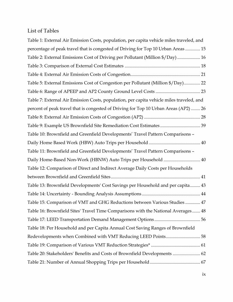
List of Tables

Table 1: External Air Emission Costs, population, per capita vehicle miles traveled, and

percentage of peak travel that is congested of Driving for Top 10 Urban Areas ............. 15 

Table 2: External Emissions Cost of Driving per Pollutant (Million $/Day) .................... 16 

Table 3: Comparison of External Cost Estimates .................................................................. 18 

Table 4: External Air Emission Costs of Congestion............................................................. 21 

Table 5: External Emissions Cost of Congestion per Pollutant (Million $/Day) .............. 22 

Table 6: Range of APEEP and AP2 County Ground Level Costs ....................................... 23 

Table 7: External Air Emission Costs, population, per capita vehicle miles traveled, and

percent of peak travel that is congested of Driving for Top 10 Urban Areas (AP2) ........ 26 

Table 8: External Air Emission Costs of Congestion (AP2) ................................................. 28 

Table 9: Example US Brownfield Site Remediation Cost Estimates ................................... 39 

Table 10: Brownfield and Greenfield Developments’ Travel Pattern Comparisons –

Daily Home Based Work (HBW) Auto Trips per Household ............................................. 40 

Table 11: Brownfield and Greenfield Developments’ Travel Pattern Comparisons –

Daily Home-Based Non-Work (HBNW) Auto Trips per Household ................................ 40 

Table 12: Comparison of Direct and Indirect Average Daily Costs per Households

between Brownfield and Greenfield Sites .............................................................................. 41 

Table 13: Brownfield Developments' Cost Savings per Household and per capita ......... 43 

Table 14: Uncertainty - Bounding Analysis Assumptions ................................................... 44 

Table 15: Comparison of VMT and GHG Reductions between Various Studies ............. 47 

Table 16: Brownfield Sites' Travel Time Comparisons with the National Averages ....... 48 

Table 17: LEED Transportation Demand Management Options ........................................ 56 

Table 18: Per Household and per Capita Annual Cost Saving Ranges of Brownfield

Redevelopments when Combined with VMT Reducing LEED Points .............................. 58 

Table 19: Comparison of Various VMT Reduction Strategies* ........................................... 61 

Table 20: Stakeholders' Benefits and Costs of Brownfield Developments ........................ 62 

Table 21: Number of Annual Shopping Trips per Household ............................................ 67 

x

Table 22: VMT Saved as a Result of Retail Brownfield/Infill Developments in Allegheny

County ......................................................................................................................................... 68 

Table 23: Average Annual Household Savings from Retail Brownfield Developments . 70 

Table 24: Average Annual Cost Saving Comparison between Residential and Retail

Brownfield Developments per Household ............................................................................ 71 

Table 25: Cycle Lengths and Peak Periods in Cranberry Township .................................. 80 

Table 26: Total Direct and Indirect Annual Costs Associated with Driving Along

Arterials in Cranberry Township ............................................................................................ 82 

Table 27: External Emissions Cost of Driving per Pollutant (1000$/Year) ....................... 82 

Table 28: List of HOT Lane Project in the U.S. Source: [124, 125] ....................................... 88 

Table 29: Environmental Costs of Driving and Congestion in the US (APEEP Model) 126 

Table 30: Environmental Costs of Driving and Congestion in the U.S. (AP2) ................ 130 

Table 31: Brownfield and Greenfield Residential Sites ...................................................... 134 

xi

List of Figures

Figure 1: Trend and Projection of Light Duty Vehicles Travel Demand in the US (1980 -

2040) [9,10]..................................................................................................................................... 4 

Figure 2: Some Components of Supply and Demand ............................................................ 5 

Figure 3: Total External Air Emissions Cost of Driving for each Urban Area .................. 16 

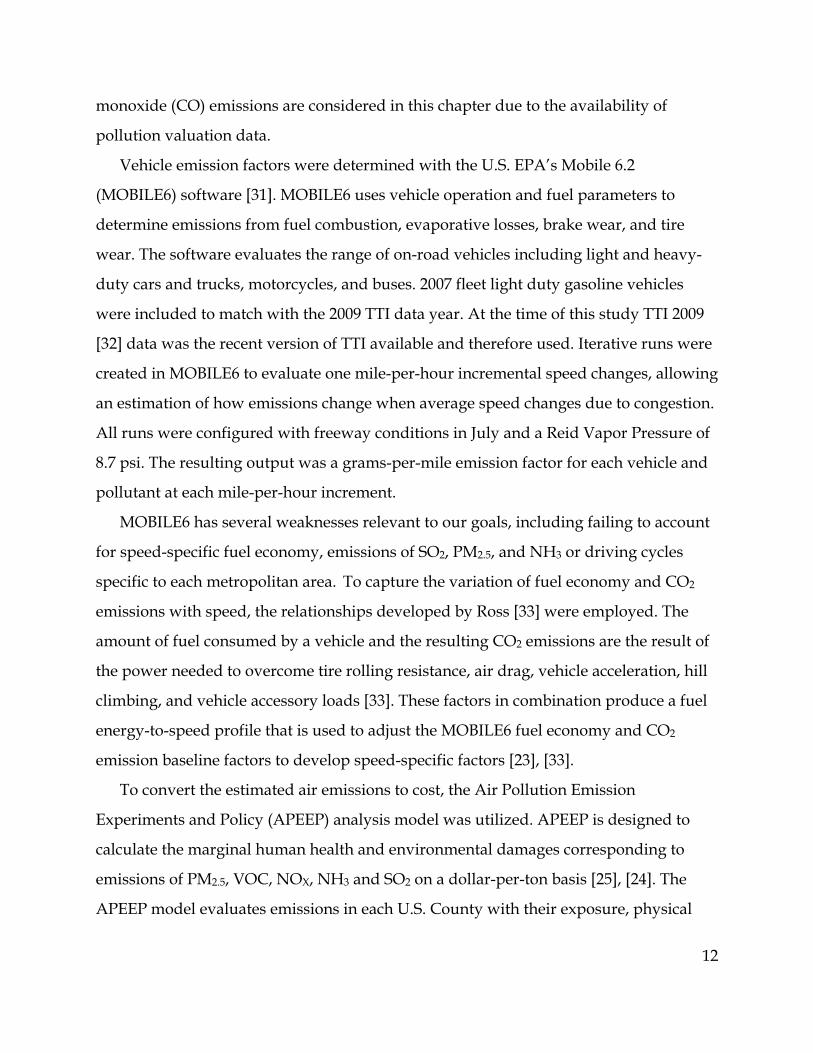
Figure 4: Total External Air Emissions Cost of Driving for each Urban Area ($/VMT) . 17 

Figure 5: Total External Air Emissions Cost of Congestion for each Urban Area (Million

$/Day) ......................................................................................................................................... 22 

Figure 6: Total External Air Emissions Cost of Congestion for each Urban Area

($/VMT) ...................................................................................................................................... 22 

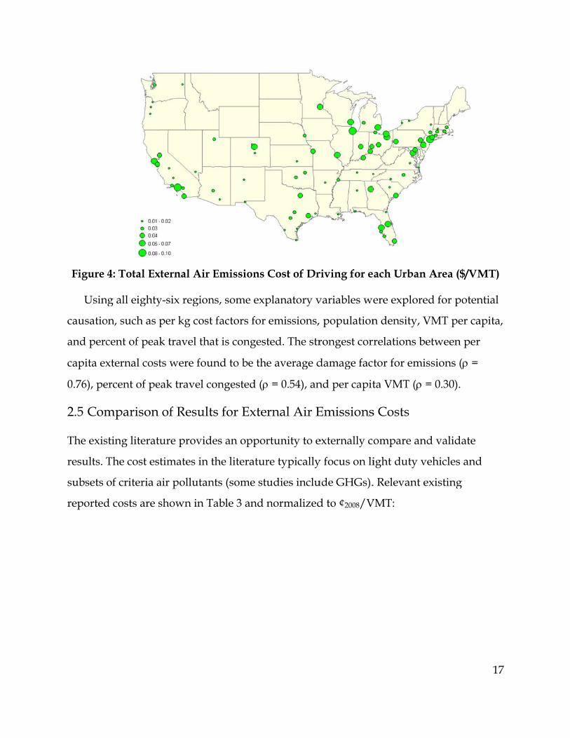
Figure 7: Cost of Driving and Congestion Comparison between APEEP and AP2 ......... 25 

Figure 8: Direct and External Environmental Costs Comparison Results between

Brownfield and Greenfield Residential Developments ........................................................ 42 

Figure 9: Sensitivity Analysis Results for Total Costs (Cost Savings) of Brownfield

Developments ............................................................................................................................. 45 

Figure 10: Net Present Value Analysis for the Base, Best and Worst Case Scenarios

(Comparison of Remediation Cost and Other Cost Savings) .............................................. 46 

Figure 11: Home Based Work (HBW) Daily VMT vs. Density ............................................ 49 

Figure 12: Location and Linkages Category under LEED for Homes Rating System [75]

....................................................................................................................................................... 53 

Figure 13: Location of Retail Stores within Alleghany County, PA ................................... 65 

Figure 14: Higher density of stores result in fewer miles saved. ........................................ 68 

Figure 15: Average Annual External Environmental Cost Savings per Household due to

Retail Brownfield by Pollutant ................................................................................................. 71 

Figure 16: Map of Cranberry Township Traffic Signal Zone, Source: [119] ...................... 79 

Figure 17: Estimated Fuel and Environmental Air Emissions Cost Savings Resulting

from Adaptive Signal Control System in Cranberry Township ......................................... 86 

Figure 18: SR167 HOT Lane Project Area, State of Washington Source: [126] .................. 89 

xii

Figure 19: Fuel and Environmental Cost Savings Resulting from SR167 HOT Lanes in

the State of Washington ............................................................................................................ 91 

Figure 20: Emissions for Various Speed Profiles ................................................................... 93 

Figure 21: Demand and Supply Changes Due to Implementation of a Congestion

Management Measure ............................................................................................................... 98 

Figure 22: Existing Travel Demand Elasticity Assessments .............................................. 100 

Figure 23: Travel Time and Delay Changes with respect to Induced Demand .............. 102 

Figure 24: Elasticity of Demand with respect to Travel Time ........................................... 102 

Figure 25: Relationship between Transportation Measures to Achieve Urban

Environmental Sustainability ................................................................................................. 108 

Figure 26: Marginal Damages for PM2.5 Sources ($/ton) from APEEP [25] .................... 125 

Figure 27: Equivalent Sources for PM2.5 Marginal Damage [34] ....................................... 125 

xiii

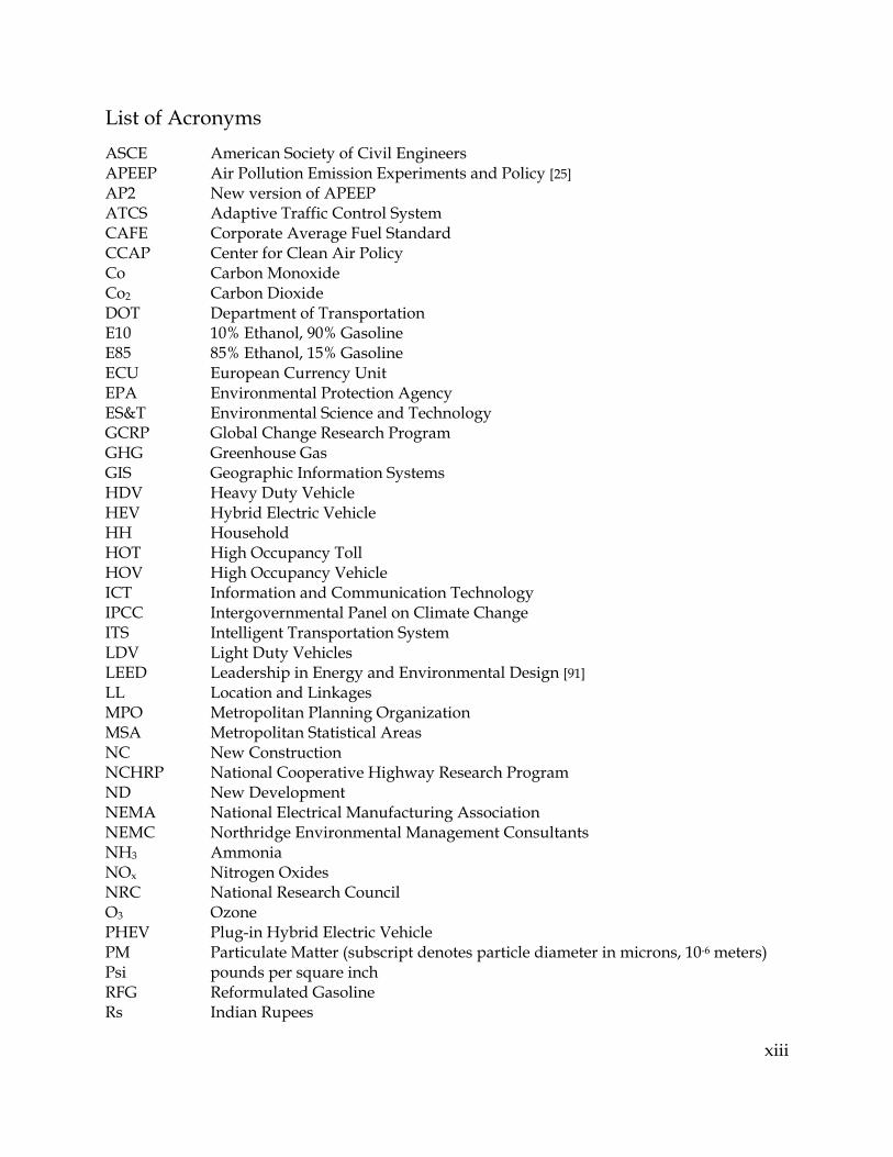
List of Acronyms

ASCE American Society of Civil Engineers APEEP Air Pollution Emission Experiments and Policy [25] AP2 New version of APEEP ATCS Adaptive Traffic Control System CAFE Corporate Average Fuel Standard CCAP Center for Clean Air Policy Co Carbon Monoxide Co2 Carbon Dioxide DOT Department of Transportation E10 10% Ethanol, 90% Gasoline E85 85% Ethanol, 15% Gasoline ECU European Currency Unit EPA Environmental Protection Agency ES&T Environmental Science and Technology GCRP Global Change Research Program GHG Greenhouse Gas GIS Geographic Information Systems HDV Heavy Duty Vehicle HEV Hybrid Electric Vehicle HH Household HOT High Occupancy Toll HOV High Occupancy Vehicle ICT Information and Communication Technology IPCC Intergovernmental Panel on Climate Change ITS Intelligent Transportation System LDV Light Duty Vehicles LEED Leadership in Energy and Environmental Design [91] LL Location and Linkages MPO Metropolitan Planning Organization MSA Metropolitan Statistical Areas NC New Construction NCHRP National Cooperative Highway Research Program ND New Development NEMA National Electrical Manufacturing Association NEMC Northridge Environmental Management Consultants NH3 Ammonia NOx Nitrogen Oxides NRC National Research Council O3 Ozone PHEV Plug-in Hybrid Electric Vehicle PM Particulate Matter (subscript denotes particle diameter in microns, 10-6 meters) Psi pounds per square inch RFG Reformulated Gasoline Rs Indian Rupees

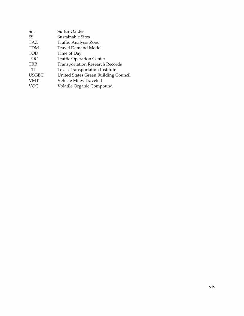
xiv

Sox Sulfur Oxides SS Sustainable Sites TAZ Traffic Analysis Zone TDM Travel Demand Model TOD Time of Day TOC Traffic Operation Center TRR Transportation Research Records TTI Texas Transportation Institute USGBC United States Green Building Council VMT Vehicle Miles Traveled VOC Volatile Organic Compound

1

Chapter 1

Introduction

1.1 Research Motivation

Modern societies rely extensively on urban transportation systems. Seamless and

efficient operation of transportation systems significantly contributes to the economic

and social wellbeing of the societies. Similar to any human developed system, urban

transportation system comes with a number of negative secondary impacts. Driving

results in approximately 10 million accidents and 39,000 deaths each year [1]. Roadway

vehicles’ air pollution cost Americans $53 billion annually even with extensive emission

control systems [2]. Noise pollution, petroleum dependence and urban sprawl are

among other negative externalities of driving [3].

Responsible for an extra 4.8 billion of travel hours and an extra 1.9 billion gallons of

purchased fuel, traffic congestion is also another negative secondary impact of driving

[4] . Traffic congestion has become a major environmental, economic and social problem

costing Americans $101 billion in 2010 [4]. These figures translate to about 34 hours of

wasted time and the average cost of about $700 per automobile commuter in one year

[4]. To promote urban environmental sustainability, greenhouse gas (GHG) and air

pollution emissions resulted from driving and traffic congestion need to be reduced

significantly. Accounting for about 30 percent of the total U.S. GHG, the transportation

sector is the second largest source of GHG in the United States [5]. Highway vehicles

including light duty vehicles (LDV), heavy trucks and buses, account for over 80

percent of transportation energy use and GHG emissions [6]. The environmental

impacts of the U.S. surface transportation system have motivated the policy world to

develop legislation supporting low carbon fuels, high efficiency vehicles and travel

reduction activities. As a result of the Energy Independence and Security Act of 2007

[7], The U.S. Department of Transportation (DOT) in coordination with the U.S.

Environmental Protection Agency (EPA) and the U.S. Global Change Research Program

(GCRP) were directed to conduct a study of the impacts of the U.S transportation

2

system on GHG emissions. As part of the mandate the responsible organizations had to

introduce and assess strategies to mitigate the negative impacts of the transportation

system on climate change [8]. The study looked at four groups of strategies that could

potentially reduce the impact of surface transportation system on GHG emissions:

1- Low carbon fuels

2- Increased vehicle fuel economy

3- Improved system efficiency

4- Reduced travel activity

This thesis mainly focuses on traffic congestion and its consequential environmental

impacts. The latter two categories mentioned above; improved system efficiency and

reduced travel activity, will be examined with respect to traffic congestion. The

objective is to estimate each category’s environmental and economic benefits and costs

using scenario based analyses and to explore and quantitatively evaluate the

interdependencies in between the two categories also known as rebound effects.

Although over 20 percent of generated GHG emissions resulted from buses and heavy

trucks, this thesis only focuses on the remaining 60 percent of highway vehicles

categorized as LDV. The goal of this work is to evaluate and to estimate monetary

values of external costs and benefits of land use and congestion management measures

in terms of environmental and health benefits and damages. In addition, while many

studies have evaluated the potential impacts of transportation mitigation measures on

GHG emission in isolation, this study combines a range of land use and congestion

management measures to prepare reasonable pathways towards urban environmental

sustainability. The hypothesis is that no one strategy, whether land use or congestion

management, will be enough to achieve urban environmental sustainability; rather it is

the net impact of strategies and the synergies between them that can potentially

produce significant impacts.

3

1.2 Research Topics

This work quantitatively and qualitatively examines the role of land use and congestion

management measures to promote urban environmental sustainability. The issues

mentioned as part of the introduction are discussed in the following chapters in greater

details. Each chapter addresses the following research topics:

Chapter 2 discusses the external environmental costs of traffic congestion in the U.S.

Chapter 3 discusses the role of land use and demand management strategies to

promote urban environmental sustainability. Specific strategies included in this chapter

are infill and brownfield developments as well as transportation smart growth

principles deployed as part of building standards.

Chapter 4 discusses the role of a number of supply management strategies in

promoting urban environmental sustainability. Specific strategies included in this

chapter are signal timing and coordination, high occupancy toll lanes and adaptive

signal timing.

Chapter 5 discusses rebound effects associated with congestion management

measures. A Specific scenario discussed in this chapter is induced demand from

roadway capacity increase resulted from proactive signal timing and coordination.

Chapter 6 of this work summarizes the findings and provides commentary on the

potential contributions of urban congestion management as a small “wedge strategy” to

attain GHG emission reduction goals relative to other transportation strategies such as

direct emissions controls. This last chapter includes suggestion for future work related

to the analyses conducted as part of this work.

Results of this work thus far have been reported in a variety of peer reviewed

journals including ASCE Journal of Urban Planning and Development, Environmental

Science and Technology (ES&T), and Transportation Research Record (TRR). Detailed

description of these articles and those coming forward is listed as part of Chapter 6.

1.3 Res

Travel in

light-du

approxim

It is proj

percent

The p

economy

with the

GHG re

applicab

vehicles

the cons

rebound

economy

uncertai

Chapter

Figu

search Bac

n the U.S. h

uty vehicle m

mately 3 tri

jected that V

over the ne

projected im

y and altern

e new Corp

duction tar

ble to the ne

) to be repl

sumer side

d effects, wh

y with extr

in at this po

r 6.

ure 1: Trend

ckground

has been inc

miles travel

illion, trans

VMT will c

ext thirty ye

mpact from

native fuels

orate Avera

rgets will be

ewly purch

aced. Due t

on replacin

hich may ca

a VMT. Ov

oint of time

d and Proje

creasing ov

led (VMT)

slating to an

continue to

ears, resulti

m increasing

s, resulting

age Fuel Ef

e difficult. T

hased vehicl

to the price

ng the used

ause the dr

verall, net be

. These stra

ection of Li(1980

ver the past

in the U.S.

n average a

increase at

ing in VMT

g VMT may

in a net inc

fficiency (C

The new 20

les and it w

e increase, th

cars with t

ivers to off

enefits of th

ategies will

ight Duty V0 - 2040) [9,

two decad

increased f

annual incre

t an average

T of 3.8 trilli

y outpace g

crease in GH

CAFE) stand

025 CAFE st

will take tim

there might

the new car

fset the savi

he new CA

be discuss

Vehicles Tr,10]

des. From 19

from about

ease of abo

e annual ra

ion by 2040

ains from im

HG emissio

dards [12, 1

tandards w

me for the ol

t be strong h

rs. Also the

ings from th

AFE standar

ed in greate

ravel Dema

992 to 2009,

2.2 trillion

ut 2 percen

ate of 1.3

0 [10].

mproved fu

ons [11]. Ev

3], reaching

will be

ld fleet (use

hesitancy fr

re are issue

he fuel

rds are high

er detail in

and in the U

4

,

to

nt [9].

uel

ven

g

ed

rom

es of

hly

US

To al

strategie

manage

(i.e. land

efficienc

improve

congesti

transpor

seconda

supply c

the capa

signal co

Reducin

transpor

parking

own cos

lleviate GH

es improvin

ment meas

d use strate

cy of transp

e mobility w

ion. The sec

rtation ther

ary impacts

can be achie

acity of road

oordination

ng demand

rt (i.e. publi

pricing, co

sts and bene

HG emission

ng the effici

ures) as we

gies) can be

portation sy

while reduc

cond set of

refore reduc

such as con

eved throu

dways by a

n, adaptive

can be achi

ic transit, b

ordon pricin

efits, they a

Figure 2: SCo

ns resulted

iency of the

ell as imple

e effective.

ystems, prov

cing GHG e

strategies p

cing deman

ngestion an

gh develop

adding lane

signal timi

ieved throu

biking, walk

ng and telec

are intercon

ome Compongestion M

from the in

e transporta

mentation

The first se

vides addit

emissions re

provides alt

nd and trav

nd GHG em

ping infrastr

es or implem

ng, or high

ugh measur

king) or imp

commuting

nnected.

ponents of Manageme

ncreased VM

ation system

of strategie

et of strateg

tional supp

esulted from

ternatives t

vel activity a

missions. Pr

ructure (i.e

menting con

h occupancy

res that imp

plementing

g. While eac

Supply andent Measure

MT, implem

m (i.e. cong

es reducing

gies, those im

ply for trave

m idling in

to automob

and the con

roviding an

e. roadways

ngestion m

y vehicle (H

prove other

g strategies

ch of the ca

d Demand es

mentation o

gestion

g travel dem

mproving t

elers to

n traffic

bile

nsequential

nd managin

s), increasin

measures suc

HOV) lanes

r modes of

such as

ategories ha

5

of

mand

the

l

ng

ng

ch as

.

as its

6

For instance, reducing transportation demand and travel activity on a regional scale

through land use strategies (i.e. shifting population growth from suburban to urban

areas) can add significant traffic congestion on local roads. In contrast, reducing travel

demand in congested urban areas can be an effective way of reducing congestion and

its consequential air emissions. In addition, reducing demand and congestion can

generate induced traffic and demand calling for further travel reduction measures.

Figure 2 illustrates some of the components of urban transportation environmental

sustainability and the linkages between the two categories of increasing supply and

reducing demand resulting in reduced traffic congestion and its consequential GHG

and air emissions. Assessing each of the components and the links in between them is

crucial in promoting and further improving urban environmental sustainability.

7

“You hit the brakes for a second, just tap them on the freeway, you can literally track the ripple effect of that action across a two hundred mile stretch of road, because traffic has a memory. It’s amazing. It’s like a living organism.”

-Mission: Impossible III

8

Chapter 2

External Environmental Cost of Congestion in the U.S.

2.1 Introduction

The modern U.S. urban transportation system has been a resounding success in

providing mobility to residents and businesses [14, 15]. Nonetheless, there are

continuing concerns for secondary effects including accidents, air emissions, congestion,

lack of physical exercise, mobility for those without motor vehicles, noise, petroleum

dependence, and urban sprawl [16-19]. Previous work has estimated the costs of some

of these externalities, notably congestion and accidents [4],[20]. In this chapter, the

external costs of air pollutant emissions from light duty vehicles (LDV) in eighty-six

major U.S. metropolitan areas, both in total for all urban travel and for the specific air

emission costs due to congestion will be estimated. Quantifying these external costs can

allow society to better understand the total costs of driving. In addition, identifying the

external costs associated with congestion can lead to a better understanding of the total

benefits that result from congestion management strategies (Chapters 3 and 4).

Urban air pollution from private vehicles has been declining since the 1970s [21],

[22], [23], even as the number of vehicles and vehicle miles traveled (VMT) in the U.S.

have been increasing [9]. These reductions in overall and per-VMT criteria air emissions

have resulted from the introduction of emission regulations and the resulting

implementation of exhaust controls. In 2009, for example, only one county in the U.S.

(Clark County, NV) had carbon monoxide levels exceeding the National Ambient Air

Quality Standard [24], a significant improvement from 1995 when 42 areas exceeded the

8-hour Standard [5]. At the same time, however, carbon dioxide emissions from private

vehicles have been growing: motor vehicle fuel economy, which determines carbon

dioxide emissions, has not had major improvements, and emissions regulation has not,

until recently, targeted carbon dioxide [5]. In 2010, the transportation sector accounted

for approximately 30 percent of total carbon dioxide emissions from fossil fuel

combustion in the U.S., of which about 60 percent resulted from gasoline consumption

9

of personal vehicles [5]. Total CO2 emissions from the transportation sector are also

growing more quickly than other sources of emissions, increasing 12 percent from 1990

to 2010 [5].

Due to the extensive U.S. effort for emission controls on motor vehicles from the

1970s onwards, external air emission costs are small relative to the overall cost of motor

vehicle use including ownership, fuel, insurance, and depreciation. For example, in

2007 dollars, the National Research Council (NRC) estimated that external health effects

for criteria air emissions (including SOX, NOx, CO, PM, VOC and NH3) was 1.3 to 1.4

cents per VMT for automobiles using gasoline (and 10 percent ethanol RFG E10) [24].

Other vehicle fuels had similarly low external costs, ranging from 1.1 to 1.2 cents per

VMT for compressed natural gas to 1.5 to 1.6 cents per VMT for hybrid electric vehicles.

Yet while the costs of external air emissions are small relative to the overall cost of

driving, the total external costs imposed on society are substantial. In 2009, 3 trillion

VMT [9] multiplied by the NRC [24] average external cost of 1.3 cents per VMT results

in an estimated overall external cost of $40 Billion, and this does not include the costs of

GHG emissions. Measures to reduce this social cost should be considered to decrease

this burden, particularly on those who choose not to drive and did not contribute to the

problem but must deal with the consequences.

Costs of congestion exceed these air emission external costs. The Texas

Transportation Institute (TTI) estimates that the cost of congestion was $101 billion in

2010, causing urban Americans to travel 4.8 billion hours more and to purchase an extra

1.9 billion gallons of fuel [4]. While literature such as TTI 2011 Urban Mobility Report

evaluates costs of congestion in U.S. urban areas, urban pollution costs associated with

driving and traffic congestion are not reported. The much-cited TTI report focuses

mostly on time and fuel costs, and could benefit from the inclusion of estimates of

pollution costs such as derived here.

This chapter estimates external air pollution costs of driving for eighty-six

metropolitan areas utilizing air pollution valuation data [25]. These cities were chosen

10

from the data reported by the TTI for 90 metropolitan areas [4]. Four areas from the TTI

list of 90 urban areas were excluded due to lack of air pollution valuation data. In

addition to the valuation of criteria air pollutants, carbon dioxide costs were estimated

using existing literature on the social cost of carbon. Importantly the proportion of this

external cost that is due to congestion is examined.

2.2 Existing Transportation External Cost Assessments

The external costs of air emissions have been evaluated and the majority of the

literature focuses on the U.S. and Europe. Several studies have quantified the economic

costs associated with mortality, morbidity, and environmental impacts, among other

external cost components. Small [26] evaluates the regional air pollution costs for Los

Angeles considering three main categories: mortality from particulates, morbidity from

particulates, and morbidity from ozone. In this region, the study evaluates several cost

accounting frameworks and produces a baseline estimate of 3.28 ¢1992/VMT. Mayeres

[27] develops external urban transportation costs for air pollution in addition to

accidents and noise. For Brussels, Mayeres estimates air pollution costs at 21-29

mECU1990/VKT (an ECU is a European Currency Unit which was replaced by the Euro

in 2001) for gasoline cars and 15-30 mECU1990/VKT for diesel cars. The study goes on to

develop marginal congestion cost estimates under the concept that time is lost when an

additional vehicle on the road reduces the speed to other road users. Air emissions

external costs of 0.02, 0.04, 0.36, and 0.30 £1993/VKT for diesel cars, light goods vehicles,

buses/coaches, and heavy goods vehicles are developed by Maddison [28] for the U.K.

Maddison [28] also considers congestion externalities through lost time evaluation to

road users. Focusing on particulate and ozone pollution’s contribution to mortality and

chronic illnesses, Delucchi [29] develops air pollution related costs for light and heavy

gasoline and diesel vehicles in the U.S. Additionally, Sen [30] develops external air

pollution cost estimates for Delhi at 0.28-0.31 Rs/VKT (Rs is Indian Rupees) for gasoline

cars and 1.03-2.74 Rs/VKT for diesel cars. Some of these studies also develop total cost

estimates for their region, similar to TTI [4], which reports external economic impacts in

11

the U.S. from congestion. While existing air pollution cost studies are sparse and often

rolled up into more comprehensive externality assessments (including components

such as noise, accidents, and value of time), several existing studies exist that provide

some new methodological approaches for improving cost estimates.

Two recent studies quantify air pollution costs by evaluating high-resolution

geographic-specific external cost data and improved emissions profiles that account for

variations in speed and congestion effects. By combining U.S. county-level air pollution

costs [25] and vehicle travel, NRC [24] develops external cost estimates for passenger

and freight modes for over 3,000 U.S. counties. These costs range from 1.33-1.8

¢2007/VMT for LDVs to 3.23-10.41 ¢2007/VMT for HDVs. Evaluating the San Francisco,

Chicago, and New York City regions, Chester [23] combines vehicle emission profiles

that are dependent on speed and age with travel surveys to evaluate costs. Across the

three cities and considering only private transit, the cost range from 0.5-64 ¢2008/vehicle-

trip and are further disaggregated by off-peak and peak times as well as passenger

loading. Chester [23] goes on to include indirect and supply chain life-cycle effects in

their assessment which can have larger impacts than emission from operating the

vehicle.

A comparison of this chapter and these past studies with a conversion of all costs to

2008 cents per vehicle mile of travel is presented in Section 2.5.

2.3 Method for Estimating External Air Emissions Costs

The external air emissions costs are estimated here from national vehicle emission

factors, metropolitan-specific travel data and metropolitan-specific external unit cost

damage factors. Vehicle per mile emission factors are used to build regional emissions

inventories in both uncongested and congested scenarios using travel data. These

regional inventories are then joined with unit external cost damage factors for specific

metropolitan areas to determine total damage costs. Carbon dioxide (CO2), sulfur

oxides (SOX), nitrogen oxides (NOX), particulates (PM2.5), ammonia (NH3) and carbon

12

monoxide (CO) emissions are considered in this chapter due to the availability of

pollution valuation data.

Vehicle emission factors were determined with the U.S. EPA’s Mobile 6.2

(MOBILE6) software [31]. MOBILE6 uses vehicle operation and fuel parameters to

determine emissions from fuel combustion, evaporative losses, brake wear, and tire

wear. The software evaluates the range of on-road vehicles including light and heavy-

duty cars and trucks, motorcycles, and buses. 2007 fleet light duty gasoline vehicles

were included to match with the 2009 TTI data year. At the time of this study TTI 2009

[32] data was the recent version of TTI available and therefore used. Iterative runs were

created in MOBILE6 to evaluate one mile-per-hour incremental speed changes, allowing

an estimation of how emissions change when average speed changes due to congestion.

All runs were configured with freeway conditions in July and a Reid Vapor Pressure of

8.7 psi. The resulting output was a grams-per-mile emission factor for each vehicle and

pollutant at each mile-per-hour increment.

MOBILE6 has several weaknesses relevant to our goals, including failing to account

for speed-specific fuel economy, emissions of SO2, PM2.5, and NH3 or driving cycles

specific to each metropolitan area. To capture the variation of fuel economy and CO2

emissions with speed, the relationships developed by Ross [33] were employed. The

amount of fuel consumed by a vehicle and the resulting CO2 emissions are the result of

the power needed to overcome tire rolling resistance, air drag, vehicle acceleration, hill

climbing, and vehicle accessory loads [33]. These factors in combination produce a fuel

energy-to-speed profile that is used to adjust the MOBILE6 fuel economy and CO2

emission baseline factors to develop speed-specific factors [23], [33].

To convert the estimated air emissions to cost, the Air Pollution Emission

Experiments and Policy (APEEP) analysis model was utilized. APEEP is designed to

calculate the marginal human health and environmental damages corresponding to

emissions of PM2.5, VOC, NOX, NH3 and SO2 on a dollar-per-ton basis [25], [24]. The

APEEP model evaluates emissions in each U.S. County with their exposure, physical

13

effects, and the resulting monetary damages. APEEP evaluates emissions at different

release heights and the ground level subset is used to evaluate vehicle effects. For each

county and each pollutant, APEEP estimates mortality, morbidity, and environmental

(e.g., crop loss, timber loss, materials depreciation, visibility, forest recreation) damages.

APEEP factors for a value of statistical life of $6M are used in this chapter. Some

metropolitan areas included in the study encompass more than one county. For these

areas, population weighted average APEEP factors are determined. For the current

status of the APEEP model, how it recently (2011) [34] changed from what was used in

this study and in general more detailed on APEEP refer to Section 2.7 and Appendix A.

The cost of CO, since not provided by APEEP, was assumed to be $520/ton [35].

This value was regionally scaled for each urban area analyzed using the ratios for NOx

observed in the APEEP data, since both pollutants are predominantly tropospheric

ozone precursors. In section 2.7, where the updated results of this analysis based on the

new APEEP costs are presented, cost of CO is benchmarked with PM10 emissions vs.

NOx. This is because CO, similar to PM10 is primarily linked to cardiovascular effects

[36].

CO2 costs are based on a literature survey performed by NRC [24]. A summary of

CO2-eq units costs from roughly 50 studies shows a median cost of $10/ton, mean cost

of $30/ton, and 5th and 95th percentile costs of $1 and $85/ton [24]. The mean $30/ton

cost is implemented for vehicle CO2 emissions in this study.

Vehicle emission factors were increased by 4.9 percent annually for CO, 1.4 percent

for NOX, 4.5 percent for PM2.5 and 5.9 percent for VOCs to capture the effects of fleet age

and improving emissions trends due to more stringent emissions standards and

improved fuel programs [23]. The average vehicle age is assumed to be 5 years [37].

The above calculated emission factors and costs were then applied to the 2007 TTI

mobility data [32] for eighty-six urban areas. As previously discussed, four urban areas

in TTI were discarded due to lack of valuation data in the APEEP model. These four

urban areas are: Anchorage, Alaska, Honolulu, Hawaii, Cathedral City and Palm

14

Spring, California, Lancaster and Palmdale, California. Volume and speed (congestion

and free flow) data utilized in the TTI report were all collected from freeway operation

centers in various urban areas. TTI provides the percentage of miles travelled in each

urban area during peak times and non-peak times. For non-peak miles, free flow speeds

of 60 and 35 miles per hour (mph) for freeways and arterials, respectively, were used in

this analysis. For peak times, TTI provides the percentage of travel that is congested and

an average congested speed. Rather than unrealistically assuming constant speed under

congested conditions, it was assumed that some percentage of vehicles operating

during congested peak times drove at a stop and go speed of 5 mph and the remaining

vehicles drove close to free flow speeds (free flow speed less one mile per hour). The

percentages were estimated so that the weighted average speed matched the congested

speed given by TTI. For non-congested peak travel, free flow speeds were used.

It is important to mention in the subsequent chapters of this work (Chapters 3 and 4),

where the external environmental costs are estimated, the same method as what was

described in this section is utilized.

2.4 Results for External Air Emissions Costs

The total external air emissions costs of light duty vehicle travel for the 86 urban areas

used in this analysis is estimated to be $145 million per day in 2007 U.S. dollars. This

averages to around 1.7 million dollars per day per urban area. Normalizing the results

by population and VMT, the external cost of driving is $0.64 per person per day or $0.03

per VMT. These estimates are higher than the national average of 1.3 cents/VMT in

NRC [24] because I am only considering urban areas and I am including a cost for

carbon dioxide emissions.

Table 1 shows a subset of the urban areas with the top 10 external costs (due to a

combination of large populations and high external cost factors). The complete list of

the external air emissions costs is included in Appendix B.

15

Table 1: Estimated External Air Emission Costs, Population, per Capita Light Duty Vehicle Miles Traveled, and Percentage of Peak Travel that is Congested of Driving for Top 10 Urban Areas

Urban Area Million $/Day

$/Day/Person

$/ VMT Population

VMT/ person

% Peak travel

congested Los Angeles-Long Beach-Santa Ana CA 23 1.8 0.086 12,800,000 21 86 New York-Newark NY-NJ-CT 23 1.3 0.10 18,225,000 12 69 Chicago IL-IN 10 1.2 0.10 8,440,000 12 79 Philadelphia PA-NJ-DE-MD 4.9 0.9 0.058 5,310,000 16 63 Washington DC-VA-MD 4.6 1.1 0.057 4,330,000 19 81 San Francisco-Oakland CA 4.5 1.0 0.056 4,480,000 18 82 Atlanta GA 4.3 1.0 0.046 4,440,000 21 75 Dallas-Fort Worth-Arlington TX 4.2 0.95 0.042 4,445,000 23 66 Detroit MI 3.9 1.0 0.045 4,050,000 21 71 Houston TX 3.9 1.0 0.043 3,815,000 24 73 Total* 145 158,355,000 Average* 1.7 0.64 0.034 1,841,000 19 48 Maximum* 23.0 1.8 0.10 18,225,000 30 86 Minimum* 0.038 0.18 0.013 145,000 10 8.0

*Average, total, maximum and minimum values are for all eighty-six urban areas.

Los Angeles and New York have the largest population among the eighty-six urban

areas and their total external emissions cost, each around $23 million/day, are roughly

twice as large as the next largest cost area (Chicago, $10 million/day). After Chicago,

another halving occurs to Philadelphia, Washington DC, San Francisco, and so on. The

largest driver for having large external costs is clearly population, as 8 of the top 10

most populous metropolitan statistical areas (MSAs) are represented in the top external

cost list—only Miami and Boston MSAs are not and they represent the 12th and 13th

rank on external costs. Looking at the normalized data shows a wide variation between

the top 3 areas—Los Angeles, New York, and Chicago—and the others, though some

other areas have high per capita (Washington DC) or per VMT (Philadelphia) costs.

The differences between normalized values are attributable to population density and

the APEEP factors, which evaluate pollutant transport, chemistry, and impact on

nearby populations [25].

Table

congesti

emission

costs, wh

have low

Ta

Total

Figu

cost per

Fig

e 2 shows t

ion disaggr

ns valued a

hile three o

wer magnit

able 2: Exte

Cost of Driv

re 3 and Fig

VMT for ea

gure 3: Tota

the $145 mi

regated by p

at $30/ton a

other pollut

udes.

ernal Emiss

ving

gure 4 illus

ach urban a

al External

llion total e

pollutant fo

are compara

tants (nitrog

sions Cost CO2

32

trate the to

area.

Air Emissi(Mil

external em

or all eight-

able in exte

gen oxides,

of DrivingNOx VO

7.6 3

otal external

ions Cost ollion $/Day

missions cos

-six urban a

ernal costs t

, sulfur diox

g per PollutOCs CO

39 31

l air emissio

of Driving y)

st of driving

areas. Carb

to VOCs, C

xide and pa

tant (MillioSOx

0.65

on costs of

for each Ur

g and

bon dioxide

CO and NH3

articulates)

on $/Day) PM NH3

3.4 31

driving an

rban Area

16

e

3

3

d

Figure

Usin

causatio

and perc

capita ex

0.76), pe

2.5 Com

The exis

results. T

subsets

reported

4: Total Ex

ng all eighty

on, such as p

cent of peak

xternal cost

ercent of pe

mparison

sting literatu

The cost est

of criteria a

d costs are s

xternal Air E

y-six region

per kg cost

k travel tha

ts were fou

eak travel co

of Result

ure provide

timates in t

air pollutan

shown in T

Emissions

ns, some exp

factors for

at is congest

nd to be th

ongested (

s for Exte

es an oppor

the literatur

nts (some st

able 3 and

Cost of Dr

planatory v

emissions,

ted. The str

e average d

= 0.54), an

rnal Air E

rtunity to e

re typically

udies inclu

normalized

riving for e

variables we

population

rongest cor

damage fac

nd per capit

Emissions

externally c

y focus on li

ude GHGs).

d to ¢2008/V

ach Urban

ere explore

n density, V

relations be

tor for emis

ta VMT ( =

s Costs

ompare an

ight duty v

. Relevant e

VMT:

Area ($/VM

ed for poten

VMT per ca

etween per

ssions ( =

= 0.30).

d validate

vehicles and

existing

17

MT)

ntial

apita,

r

d

18

Table 3: Comparison of External Cost Estimates

Study Geographic Area

Vehicle Set Air Pollutants Included

Cost in ¢2008/VMT

This Study U.S. Urban Areas

LDVs CO2, CO, NOX, SO2, PM2.5, VOCs, NH3 1.15 – 10.28

[26] Los Angeles Region, U.S.

LDGVs NOX, SOX, PM10,

VOCs 2.12 - 18.28

[27] Brussels, Gasoline Cars

Diesel Cars

CO2, CO, NOX, SOX, 7.25 - 11.51

5.28 - 10.37

[28] U.K. Diesel Cars NOX, SOX, PM10, VOCs (+Benzene), Lead

2.80

[16] U.S. LDGVs O3, CO, NO2, PM, Toxics 0.89 - 11.83

[30] Delhi, India Gasoline Cars CO, NOX, PM, HC 1.07 - 1.23

Diesel Cars 4.09 - 10.87

[24] U.S. Counties LDAs NOX, SOX, PM2.5, VOCs 1.37 - 1.87

[23] San Francisco, Chicago, & New York City, U.S.

LDVs GHGs, CO, NOX, SO2, PM10, VOCs 2.70 - 3.50

Notes: All costs are adjusted to ¢2008 based on USBLS [38]. Currency conversion factors of 1.7 £1993 per $1993, 1.3 ECU1990 per $1990, and 44 Rs2005 per $2005 are used. (1) The Delucchi [16] cost range is for vehicle emissions while the study also reports upstream impacts. (2) The Chester [23]cost range is for vehicle emissions only while the study also reports life-cycle emissions and associated costs.

The variation in estimates in the literature can be the result of many factors. The

differing temporal and geographic boundaries imply varying vehicle emissions profiles.

The vehicle fleet sets evaluated can also change emission profiles. Most studies

acknowledge the uncertainty in estimating mortality and morbidity costs including the

effects of using different values of statistical life. The air pollutant damages considered

across the studies are also inconsistent. Some studies include human health impacts

only while others capture climate, vegetation, visibility, material, and aquatic damages

as well. While these factors lead to an inconsistency in external cost comparisons, the

literature results produce a range of 5.1±4 ¢2008/VMT. This range is consistent with the

results of this study at 1.15-10.28 ¢2008/VMT.

19

2.6 Estimation of External Air Emissions Costs Due to Congestion

By disaggregating congestion costs from total costs, external cost estimates associated

with low-speed and higher per-VMT emissions were assessed. To calculate this cost, a

non-congested scenario in which all miles in the urban areas are driven at free flow

speeds was established as a baseline. The difference between the costs of this non-

congested scenario and the existing costs of pollution at congested speed provides an

estimate of the incremental external cost of congestion. Using a speed distribution

profile where a fraction of vehicles drive at 5 mph during congested peak times and the

remaining vehicles drive close to free flow speed, a weighted average congestion speed

was determined that matches those reported by TTI [32]. This method is believed to

provide a more realistic and accurate result than assuming a single congested speed

applies to all vehicles driving during congested times.

20

Table 4 shows comparable estimates for the external air emissions costs due solely to

congestion in urban areas. The total estimate of $24 million/day due to congestion is a

portion of the $145 million/day in total external emission costs. These amounts are

relatively small compared to travel time costs of congestion since emissions do not vary

substantially with changes in average speeds. However, this small variation may be

due to limitations in the MOBILE 6 model—as discussed above many of the emissions

factors do not vary with speed. Nevertheless, they represent savings that could be

realized in at least some portion by effective congestion management schemes. The

complete list of the external air emissions costs is included in Appendix B.

21

Table 4: External Air Emission Costs of Congestion

Urban Area Million $/Day

$/Day/Person

$/ VMT

Population VMT/ person

% Peak travel

congested Los Angeles-Long Beach-Santa Ana CA 5.3 0.42 0.020 12,800,000 21 86 New York-Newark NY-NJ-CT 4.4 0.24 0.020 18,225,000 12 69 Chicago IL-IN 1.3 0.15 0.012 8,440,000 12 79 San Francisco-Oakland CA 0.95 0.21 0.012 4,480,000 18 82 Washington DC-VA-MD 0.87 0.20 0.011 4,330,000 19 81 Atlanta GA 0.77 0.17 0.008 4,440,000 21 75 Houston TX 0.73 0.19 0.008 3,815,000 24 73 Dallas-Fort Worth-Arlington TX 0.72 0.16 0.007 4,445,000 23 66 Miami FL 0.71 0.13 0.008 5,420,000 17 82 Philadelphia PA-NJ-DE-MD 0.69 0.13 0.008 5,310,000 16 63 Total* 24 158,355,000 Average* 0.28 0.08 0.004 1,841,000 19 48 Maximum* 5.3 0.42 0.02 18,225,000 30 86 Minimum* 0.03 0.0042 0.000 145,000 10 8.0 *Average, total, maximum and minimum values are for all 86 urban areas.

The top 10 highest external congestion cost cities are clearly quite similar to total

costs—9 of the top 10 are on both lists. In terms of congestion Los Angeles and New

York score high above all other cities, particularly related to per capita external costs

where Los Angeles nearly doubles its closest competitor, $0.42/person-day compared

to second-ranking New York at $0.24/person-day. As might be expected, the difference

between the maximum and minimum per capita and per VMT cost values (~2 orders of

magnitude) are higher for congestion costs than for total costs (~1 order of magnitude),

since in some cities congestion is a much larger problem than others. Calculating similar

correlations as for total costs, the most important variables explaining a high congestion

cost were percent of peak travel congested ( = 0.84), pollution cost ( = 0.76), and

population density ( = 0.52).

Table 5 shows the total external emissions cost of congestion for each specific

pollutant for all eighty-six urban areas. NH3 and VOC have the largest estimated costs

for criteria pollutants. Carbon dioxide valued at $30/mt shows the largest total of

external cost due to congestion.

Tab

Total

F

solely to

Figu

Figu

ble 5: Extern

Cost of Cong

igure 5 and

o congestion

ure 5: Total

ure 6: Total

nal Emissio

gestion

d Figure 6 g

n for each u

External A

External A

ons Cost ofCO2

9.4

graphically

urban area a

Air Emissio(Mil

Air Emissio(

f CongestioNOx VO

0.4 6

illustrate to

and the cos

ns Cost of llion $/Day

ns Cost of ($/VMT)

on per PolluOCs CO

6.9 2.0

otal externa

st per VMT

Congestiony)

Congestion

utant (MillSOx

0.0

al air emiss

T.

n for each U

n for each U

lion $/Day)PM NH

0.0 0.0

sion costs du

Urban Are

Urban Are

22

) H3

0

ue

a

a

23

2.7 Updates to the APEEP Model

Muller 2011 [34] reports that the original APEEP model [25] (used for this study thus

far), has been significantly updated by building a stochastic version of the model. The

new model is referred to as AP2. It estimates the marginal damages ($/ton) of

pollutants for 2005. Damage costs resulting from AP2 are significantly higher than those

from the original APEEP model. The distributions for the damages in AP2 are right-

skewed, especially the ground level emissions, which we used in this work for

transportation damage cost estimations. As a result, the mean from these distributions

tends to be larger than the mean from the deterministic APEEP model. In addition,

baseline emissions have changed since the development of APEEP, which causes the

marginal damages to change as well. AP2, also, uses updated mortality rate and

pollution data relative to what was used in APEEP. Therefore, damage costs resulting

from AP2 are higher than those in APEEP. Table 6 compares the mean values from AP2

versus deterministic values from APEEP:

Table 6: Range of APEEP and AP2 County Ground Level Costs

Pollutant

APEEPModel AP2ModelMean

Multiplierfrom

APEEPtoAP2

LowestCountyCost($/kg)

HighestCountyCosts($/kg)

MeanCostAcrossall

U.S.Counties($/kg)

LowestCountyCost($/kg)

HighestCountyCosts($/kg)

MeanCostAcrossall

U.S.Counties($/kg)

VOC 0.04 50 1.4 0.2 150 3.4 2.5

NOx 0.05 20 1.8 0.3 50 4 2.2

PM2.5 0.4 540 14 1.5 1,600 36 2.5

SO2 0.3 180 6 1.2 520 18 3

NH3 0.2 1,100 14 0.7 3,100 34 2.4

Table 6 illustrates that mean values across the U.S. counties are two to three

times higher in AP2 compared with those in APEEP. A complete description of both

models (APEEP and AP2) may be found in Appendix A. This section reproduces results

from the analysis described in this chapter using AP2 values. The cost of CO2, not

provided by APEEP or AP2, remained unchanged from the previous analysis and the

24

same average values were used from the existing literature [17, 35]. The cost of CO,

however, as mentioned earlier, is benchmarked with PM10 emissions vs. NOx. This is

because CO, similar to PM10 is primarily linked to cardiovascular effects [36]. For the

remainder chapters of this work APEEP values have been used. Since the variation

between APEEP and AP2 mean values is consistent throughout the counties, changes in

results based on AP2 mean values are fairly predictable. Important to note that at the

time most of the analyses in this work were done, AP2 was not available. Furthermore,

access to AP2 values currently is limited and only mean cost values are available.

Should the ranges assumed in the AP2 model become available, adding ranges to the

cost saving results estimated throughout this work may produce interesting results.

Total cost of driving per AP2 was estimated to be about $300 million per day, which

is almost twice as much as what was estimated with the original APEEP model. Of the

$300 million per day, $44 million per day is the cost of congestion. This converts to the

annual cost of driving of $110 billion and the annual congestion cost of $16 billion.

Thus, emissions due to congestion contribute roughly 18 percent of the total costs of

urban congestion when compared to the estimate of $87 billion in 2007 by TTI [32] and

15 percent of the total costs of urban congestion when compared to the estimate of $101

billion resulted from AP2 [4].

Figure 7 shows the difference of the breakdown of the costs of various pollutants

between the two models.

Figur

Table

and New

their cos

using th

whereas

higher th

Diego, C

and Hou

up amon

re 7: Cost o

e 7 is a repr

w York rem

sts of drivin

he previous

s AP2 result

han cost of

CA and Bos

uston, TX a

ng all urban

of Driving a

roduction o

main to be th

ng is signifi

model (AP

ts show the

driving in

ston, MA ar

are no longe

n areas.

and Conge

of Table 1 w

he top urba

icantly high

PEEP), cost

e cost of dri

New York

re now on t

er on the top

stion Comp

with the new

an areas on

her compar

of driving f

iving in Los

area. Using

the top ten l

p ten list. A

parison bet

w AP2 mod

the cost lis

ed with the

for both are

s Angeles a

g the AP2 m

list while A

Average cos

tween APE

del. While L

t, the differ

e previous m

eas were ab

area is abou

model, Miam

Atlanta, GA

st of driving

EEP and AP

Los Angeles

rence betwe

model. In fa

bout the sam

ut 30 percen

mi, FL, San

A, Dallas, TX

g has doub

25

P2

s

een

act

me,

nt

n

X

led

26

Table 7: External Air Emission Costs, Population, per Capita Light Duty Vehicle Miles Traveled, and Percent of Peak Travel that is Congested of Driving for Top 10

Urban Areas (AP2)

Urban Area Million $/Day

$/Day/Person

$/ VMT Population

VMT/ person

% Peak travel

congested Los Angeles-Long Beach-Santa Ana CA 75.3 5.9 0.28 12,800,000 21 86 New York-Newark NY-NJ-CT 58.6 3.2 0.26 18,225,000 12 69 Chicago IL-IN 15.0 1.8 0.14 8,440,000 12 79 San Francisco-Oakland CA 12.6 2.8 0.15 4,480,000 18 82 Philadelphia PA-NJ-DE-MD 11.3 2.1 0.13 5,310,000 16 63 Miami FL 8.8 1.6 0.09 5,420,000 17 82 San Diego CA 8.2 2.8 0.13 2,950,000 21 84 Detroit MI 8.1 2.0 0.09 4,050,000 21 71 Washington DC-VA-MD 7.8 1.8 0.09 4,330,000 19 81 Boston MA-NH-RI 5.7 1.4 0.07 4,200,000 18 58 Total* 301 158,355,000 Average* 3.5 1.08 0.06 1,841,000 19 48 Maximum* 75.3 5.9 0.28 18,225,000 29 86 Minimum* 0.03 0.16 0.01 145,000 10 8.0

*Average, total, maximum and minimum values are for all eighty-six urban areas.

27

Table 8 shows the external air emission costs of congestion for the top ten urban

areas based on the new AP2 model.

28

Table 8: External Air Emission Costs of Congestion (AP2)

Urban Area Million $/Day

$/Day/Person

$/ VMT

Population VMT/ person

% Peak travel

congested Los Angeles-Long Beach-Santa Ana CA 14.1 1.10 0.05 12,800,000 21 86 New York-Newark NY-NJ-CT 7.8 0.43 0.04 18,225,000 12 69 San Francisco-Oakland CA 2.2 0.49 0.03 4,480,000 18 82 Chicago IL-IN 1.9 0.23 0.02 8,440,000 12 79 Miami FL 1.5 0.27 0.02 5,420,000 17 82 San Diego CA 1.4 0.47 0.02 2,950,000 21 84 Philadelphia PA-NJ-DE-MD 1.4 0.26 0.02 5310,000 16 63 Washington DC-VA-MD 1.3 0.31 0.02 4,330,000 19 81 Atlanta GA 1.0 0.22 0.01 4,440,000 21 75 Detroit MI 1.0 0.24 0.01 4,050,000 21 71 Total* 44.5 158,355,000 Average* 0.28 0.13 0.01 1,841,000 19 48 Maximum* 14.1 1.10 0.05 18,225,000 29 86 Minimum* 0.002 0.005 0.001 145,000 10 8.0 *Average, total, maximum and minimum values are for all eighty-six urban areas.

Los Angeles, CA and New York, NY remain to be the top two cities when it comes

to the cost of congestion. San Francisco, CA and Chicago, IL seem to switch places on

the chart. Dallas, TX and Houston, TX are no longer among the top ten urban areas

when it comes to the external environmental cost of congestion as San Diego, CA and

Detroit, MI took their places on the list. A complete list of all eight-six urban areas and

their environmental costs of driving and congestion may be found in Appendix B.

2.8 Conclusions

In this chapter, external air emissions costs associated with light vehicle automobile

travel in urban metropolitan areas were estimated. These estimates are based on

emission factors provided by MOBILE6 and air pollution valuation data provided by

the APEEP and AP2 models. Existing average literature values [17, 35] were assumed

for costs of carbon dioxide and carbon monoxide, since not provided by the APEEP

model. The external environmental cost estimates from this chapter can be used in

benefit/cost studies to assess the benefits of travel reduction, congestion management

and the like. While other external costs such as congestion time are larger in

magnitude, the external air emission costs are still appreciable, amounting to $16 billion

29

annually with a total cost of driving estimated at $110 billion annually. Thus, emissions

due to congestion contribute roughly 18 percent of the total costs of urban congestion

when compared to the estimate of $87 billion in 2007 by TTI [32]. Efforts to rein in

congestion and decrease urban driving will clearly thus have important impacts on fuel

consumption, time, and environmental damages. Strategies that can have significant

impact on reining congestion and its consequential environmental impacts will be

assessed in Chapter 3 and Chapter 4.

30

“Everyone in New York City knows there’s gotta be way more cars than parking spaces. You see cars driving in New York all hours of the night. It’s like Musical Chairs except everybody sat down around 1964.”

-Jerry Seinfeld

31

Chapter 3

Land Use and Demand Management Strategies

3.1 Reducing Demand: Vehicle Miles Travel Reduction and Land Use

From 1992 to 2008, light durty vehicle miles traveled (VMT) in the U.S. increased from

about 2.2 trillion to approximately 3 trillion, translating to an average annual increase of

about 2 percent [9]. Projections show that VMT will continue to increase at an average

annual rate of 1.3 percent, resulting in VMT of 3.8 trillion by 2040 [10]. As it was shown

in the previous chapter, the increase in VMT results in traffic congestion which costs the

U.S. metropolitan urban areas $16 billion a year (2007) in terms of environmental

damages.

Reducing VMT and the resulting greenhouse gas (GHG) emissions can be

accomplished by various strategies including but not limited to parking management,

pricing alternatives, telecommuting, teleconferencing and public transit improvement

as well as changing land use patterns. Changing land use patterns can be accomplished

through smart growth1 concepts such as infill developments, compact developments,

mixed-used developments, walkable communities and transit-oriented developments

[39]. Compact urban development has been correlated to a reduction of 20 – 40 percent

in VMT compared to sprawl [40]. A National Research Council (NRC) study concluded

that compact developments with a high density are likely to reduce VMT, energy

consumption, and CO2 emissions [41]. Handy [42] and Shammin [43] also support the

benefits of compact developments with respect to reducing energy consumption and

travel activity. On the other hand, critics of compact developments note the costly

effects of increased traffic congestion, higher taxes, higher consumer costs and more

intensive developments ([44], [45]).

1 Smart growth promotes land use changes to encourage concentrating of growth in compact, walkable, transit oriented, 

developments and to limit sprawl.  

32

3.2 A Land Use Strategy to Reduce VMT: Brownfield Development

Large brownfield developments are typically redeveloped as mixed-use or compact

developments, which consist of residential, retail, offices, entertainment centers and

community centers. Paull [46] documents that increasing mixed-use and especially

residential use of the brownfield sites meets smart growth objectives. A number of

studies have documented that brownfield developments are mostly compact.

Brownfield developments conserve land in a ratio of 1 acre per brownfield redeveloped

to 4.5 acres per conventional greenfield [47]. De Sousa [48] reports brownfield

residential density of 59 households per acre in Chicago. In addition to density, distance

to city centers, close access to transit, diversity of land use within the developments,

and the design of the mixed-use developments, both internally and in connection with

the existing urban grids, are factors that can potentially influence the impact that

compact brownfield developments might have on VMT reduction. Several studies show

that brownfield developments lower VMT compared to conventional greenfield

developments ([49], [50], [51]). Moreover, Nagengast [52] compares commuting travel

times between brownfields and greenfields in six cities and concludes that commuting

travel time is less for brownfields compared to greenfields.

3.2.1 Brownfield Developments

Brownfields are properties for which expansion, redevelopment, or reuse may be

complicated by the presence or potential presence of hazardous substances, pollutants,

or contaminants [53]. An estimated 450,000 to 1,000,000 brownfield sites remain

abandoned across the country [54]. These sites include former industrial or

manufacturing plants, dry cleaners, gas stations, laboratories and residential buildings.

From the private developers’ perspective, brownfield sites are not the most desirable

investments, because developing brownfields incurs initial assessment and remediation

costs and involves barriers such as uncertainty about the presence and type of

contamination, uncertainty over cleanup standards, limited cleanup resources, and

33

potential liability issues [55],[56]. On the other hand, developing these underutilized

lands can positively impact economic development and the environment [57].

Brownfield developments have been shown to revive communities [58], increase

employment [48], generate local tax revenue [48], keep green spaces intact [47], and

reduce sprawl and travel activity as well as the resulting air emissions [40].

To make a proper decision about developing a brownfield site, it is important that

all benefits and costs are taken into account. In this chapter, the impact of residential

brownfield developments on travel activity reduction and the consequential costs,

including the cost of time and fuel as well as the external environmental costs, are

examined. Assessing contributing factors such as travel distance and number of trips

generated by each of the brownfield and greenfield2 sites, VMT for a sample of

brownfield and greenfield residential developments in four cities: Chicago, Pittsburgh,

Baltimore and Minneapolis are compared. In addition the external air pollution costs of

driving for each brownfield and greenfield site using air pollution valuation data are

estimated [25]. Furthermore, the environmental costs are compared with the cost of

brownfield remediation. While the VMT reduction benefits of brownfield developments

have been evaluated by a number of studies in the U.S., as will be explained, no study

to date has performed a comparison between the environmental, time and fuel benefits

of brownfield developments and the cost of remediation. My goal is to determine if the

environmental cost savings as well as time and fuel cost savings from VMT reductions

offset the extra initial onetime cleanup cost of brownfield developments. If that is the

case, this should provide motivation for collaboration between various public agencies

(i.e. DOT and EPA) to join efforts in developing residential brownfields. In the final

section, the cost-effectiveness of brownfield developments as a VMT reduction strategy

in comparison with other VMT reduction strategies is examined. To minimize the

2 Greenfields are undeveloped lands such as farmlands, woodlands, or fields located on the outskirts of urbanized 

areas (HUD, 2010). In the absence of brownfield developments, greenfield developments are where growth 

occurs. 

34

impact of the transportation sector on GHG emissions, transportation agencies have set

goals that require implementing VMT reduction strategies. Brownfield developments

can be a cost-effective strategy compared to other VMT reduction alternatives,

promoting effective VMT reduction and GHG mitigation strategies.

While most sections of this chapter and analysis strictly deal with residential

brownfields, in the last part of this chapter (Section 3.6) retail brownfields are briefly

examined. A case study of four retail brownfield sites in Alleghany County,

Pennsylvania is assessed to evaluate the impact of the retail developments on VMT

savings. Results of this analysis should provide guidance to the city authorities and

urban planners in deciding the location of the upcoming retail facilities within their

jurisdiction. The objective is to keep the environmental damages due to driving minimal

as officials are promoting the economic growth of their cities.

3.2.2 Remediation Cost of Brownfield Sites

To develop a brownfield site, a risk assessment generally followed by site remediation

is necessary. The remediation solution largely depends on the types of contaminants

found. The cost of remediation varies significantly depending on the type of

contaminant, level of exposure, and procedures needed to clean up the contaminants

([59], [60]). The Council of Urban Economic Development reports the median cleanup

cost per acre is $57,000 [61]. The City of Chicago reports the remediation cost of

multiple projects from $25,000 to $530,000 per acre [62]. A complete list of remediation

costs from multiple studies is presented in the method section of this chapter (Section

3.2.3).

Although incurring initial remediation cost, brownfield developments might require

lower initial construction investments as they are typically built compact and, in most

cases, benefit from already existing infrastructures such as water pipelines, power

supply, roadways and sewer systems ([63],[64],[65]). Opponents of brownfield

developments critique the lower initial brownfield construction investments and

believe that for sites with higher density the existing infrastructure may not be properly

35

sized or reusable, and due to brownfields’ typical location within the urban core and

scarcity of land in those areas development cost are higher ([66], [67]).

3.2.3 Method

Based on data availability, a sample of 16 U.S. brownfield and greenfield residential

developments were selected in the four metropolitan areas of Baltimore, Chicago,

Minneapolis and Pittsburgh. With the assistance of expert local representatives

managing brownfield programs and local urban planners in each of the cities, two

brownfield residential developments and two comparable greenfield residential

developments were identified in each of the four cities. Two criteria were considered in

the selection process of the sites: (1) minimum of one hundred dwelling units within

each development; and, (2) developments must have been completed within the past

twenty years. The average distance between the selected brownfield sites and city

centers is 4 miles while the average distance from the selected greenfield sites to city

centers is 21 miles. Specific information of the sites may be found in the Appendix C.

To determine the average difference in travel activities between residential

brownfield and greenfield developments, 2010 travel demand model (TDM) outputs

were obtained from the metropolitan planning organizations (MPO) for each city.

Travel demand models simulate real world travel patterns. The model takes into

account travel behaviors that influence drivers’ choice of destination, mode of

transportation and selected routes [68]. TDMs and Geographic Information Systems

(GIS) were used to identify Traffic Analysis Zones (TAZ) containing the study sites. A

Traffic Analysis Zone is the unit of geography, similar to census tracts, used in travel

demand models [69]. By analyzing trip productions and attractions3, the number of

home-based automobile trips and resulting VMTs generated and distributed by the

study sites to all other TAZs were calculated. The trips were categorized into two

3 Trip production and attraction refer to the number of trips produced and attracted to each TAZ. 

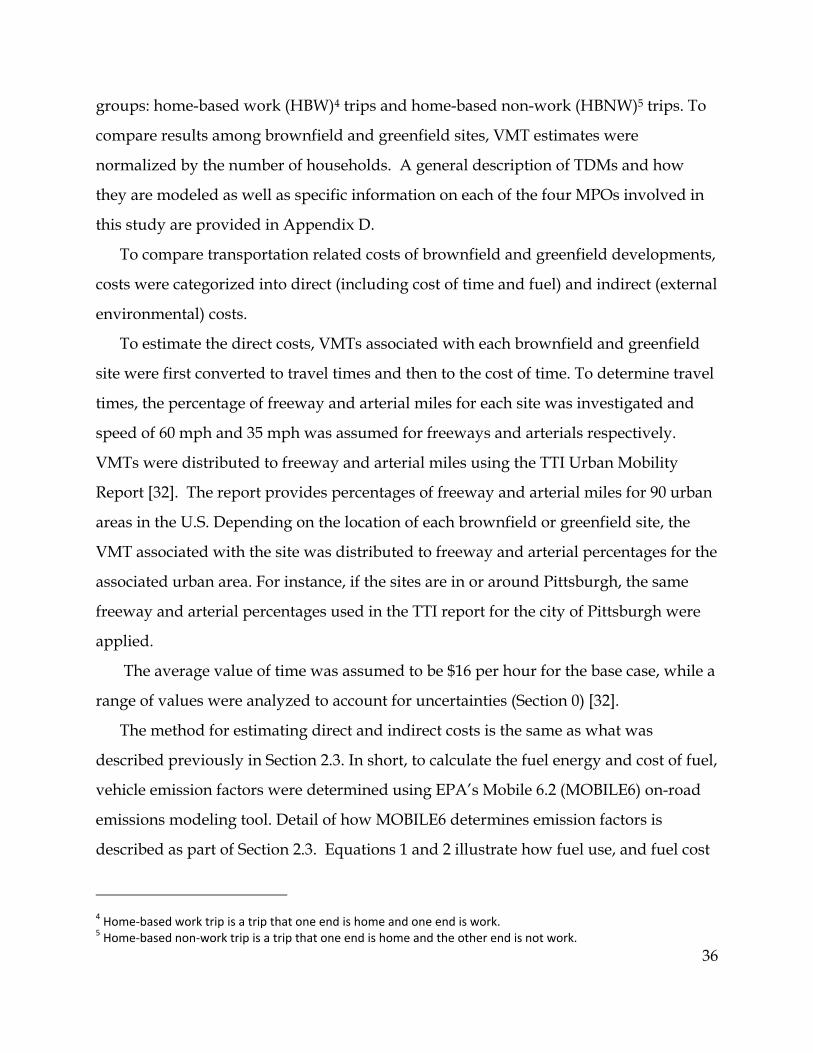
36

groups: home-based work (HBW)4 trips and home-based non-work (HBNW)5 trips. To

compare results among brownfield and greenfield sites, VMT estimates were

normalized by the number of households. A general description of TDMs and how

they are modeled as well as specific information on each of the four MPOs involved in

this study are provided in Appendix D.

To compare transportation related costs of brownfield and greenfield developments,

costs were categorized into direct (including cost of time and fuel) and indirect (external

environmental) costs.

To estimate the direct costs, VMTs associated with each brownfield and greenfield

site were first converted to travel times and then to the cost of time. To determine travel

times, the percentage of freeway and arterial miles for each site was investigated and

speed of 60 mph and 35 mph was assumed for freeways and arterials respectively.

VMTs were distributed to freeway and arterial miles using the TTI Urban Mobility

Report [32]. The report provides percentages of freeway and arterial miles for 90 urban

areas in the U.S. Depending on the location of each brownfield or greenfield site, the

VMT associated with the site was distributed to freeway and arterial percentages for the

associated urban area. For instance, if the sites are in or around Pittsburgh, the same

freeway and arterial percentages used in the TTI report for the city of Pittsburgh were

applied.

The average value of time was assumed to be $16 per hour for the base case, while a

range of values were analyzed to account for uncertainties (Section 0) [32].

The method for estimating direct and indirect costs is the same as what was

described previously in Section 2.3. In short, to calculate the fuel energy and cost of fuel,

vehicle emission factors were determined using EPA’s Mobile 6.2 (MOBILE6) on-road

emissions modeling tool. Detail of how MOBILE6 determines emission factors is

described as part of Section 2.3. Equations 1 and 2 illustrate how fuel use, and fuel cost

4 Home‐based work trip is a trip that one end is home and one end is work. 5 Home‐based non‐work trip is a trip that one end is home and the other end is not work. 

37

were estimated. Fuel use (FU) is a function of fuel energy (FE) and daily vehicle miles

traveled (DVMT) and fuel cost (FC) is a function of FU and the price of gasoline.

FU(a) = (FEi *DVMTi(a))+(FEj*DVMTj(a)) (1)

FC(a) = (FU(a) * P)/C (2)

where:

FU(a) = Fuel use for site a (MJ/day);

FE = Fuel energy (MJ/Mile);

FC(a) = Fuel cost for site a ($/day);

P = Price of gas ($2.8/gallon);

C = 121.3 MJ/gallon of gasoline

DVMT(a) = Daily vehicle miles traveled for site a (mile/day); and

i and j represent freeway and arterial respectively.

To calculate the cost of external air emissions, the APEEP model was used. The same

method as in section 2.3 was used to valuate various pollutants. In case of CO and CO2

the same values as section 2.3, $520/kg and $30/ton, were used ([17],[35],[24]). To

account for uncertainties, data ranges for the cost of CO, CO2, gas, time and APEEP

costs are assumed and will be explained in section 0.

The method used to estimate the external environmental costs is also what was

described in section 2.3. Combining the cost of each pollutant from APEEP ($/kg) with

emission factors from MOBILE6 (gram/mile) and daily VMTs (mile/day), the external

environmental cost of each pollutant was calculated for each development using the

following equation:

Ci(a) = DVMT(a) * EFi * Ci (3)

where:

Ci(a) = Cost of pollutant i for development a ($/day);

38

DVMT(a) = Daily vehicle miles traveled for development a (mile/day);

EFi = Emission factor for pollutant i (gram/mile); and

Ci = Cost factor for pollutant i ($/1000gram).

3.2.4 VMT and Remediation Cost Comparison

After direct and indirect transportation costs were calculated and compared between

the brownfield and greenfield developments, brownfield cost savings from VMT

reductions were also compared with the initial remediation cost. The goal was to

examine if the cost savings from VMT reductions offset the extra initial one-time

cleanup cost of brownfield developments.

The remediation cost depends significantly on the type of contaminant and the level

of exposure, both of which factored in selecting the strategy used to cleanup the site.

Generally one of the following remediation strategies is used for brownfield site

cleanup.

- Immobilization of the contaminants (i.e., stabilization, solidification, landfill

construction, capping, slurry walls and in-situ solidification),

- Destruction or alteration of contaminants (i.e., biodegradation, incineration, low

temperature thermal desorption),

- Removal or separation of contaminants (i.e. air stripping, ion exchange, soil

washing, soil vapor extraction, solvent extraction) [60].

The cost of cleanup includes direct costs, contractors’ overhead and profits, and

contingencies. Since these values vary significantly from site to site, a range of

remediation costs from multiple studies and references was used:

39

Table 9: Example US Brownfield Site Remediation Cost Estimates Study Remediation Cost ($/acre) Note Chicago 2003 [70] 25,000-530,000 Various Projects

Auld 2010 [71] 580,000 Pittsburgh

Lehr 2005 [72] 250,000-500,000 Capping

CUED 1999 [73] 57,000 -

R.S. Mean 2010 [74] 45,000 Capping (18”)

Terry 1999 [75] 22,000 Phytostabilization

Terry 1999 [75] 56,000 Soil Capping

Terry 1999 [75] 65,000 Asphalt Capping

To compare the one-time remediation cost with the cost savings from the VMT

reductions calculated earlier, the average cost of $190,000 per acre was used for the base

case and the 95th percentile cost of $550,000 per acre and 5th percentile cost of $24,000

per acre were used for the worst and best cases respectively. Time period of 20 years

was assumed for this analysis.

The residential density of the eight selected brownfield sites ranges from 6 to 59

households per acre with the median of 12 households per acre. Great Communities

Organization reports a range of 19 to 129 household per acre for compact

developments[76]. Leading studies in compact developments report an average of 11 to

15 households per acre for compact developments [24, 38, 40]. For this study an average

of 12 households per acre was used to normalize the base remediation cost.

3.2.5 VMT Comparison Results for Brownfield and Greenfield Sites

VMTs were calculated for eight brownfield and eight greenfield sites within the four

selected cities of Baltimore, Chicago, Minneapolis and Pittsburgh.

Table10 compares HBW automobile VMTs, trip distance and the number of trips per

household for brownfields and greenfields.

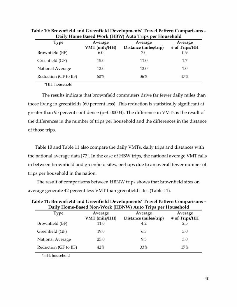
40

Table 10: Brownfield and Greenfield Developments’ Travel Pattern Comparisons – Daily Home Based Work (HBW) Auto Trips per Household

Type Average VMT (mile/HH)

Average Distance (miles/trip)

Average # of Trips/HH

Brownfield (BF) 6.0 7.0 0.9

Greenfield (GF) 15.0 11.0 1.7

National Average 12.0 13.0 1.0

Reduction (GF to BF) 60% 36% 47%

*HH: household

The results indicate that brownfield commuters drive far fewer daily miles than

those living in greenfields (60 percent less). This reduction is statistically significant at

greater than 95 percent confidence (p=0.00004). The difference in VMTs is the result of

the differences in the number of trips per household and the differences in the distance

of those trips.

Table 10 and Table 11 also compare the daily VMTs, daily trips and distances with

the national average data [77]. In the case of HBW trips, the national average VMT falls

in between brownfield and greenfield sites, perhaps due to an overall fewer number of

trips per household in the nation.

The result of comparisons between HBNW trips shows that brownfield sites on

average generate 42 percent less VMT than greenfield sites (Table 11).

Table 11: Brownfield and Greenfield Developments’ Travel Pattern Comparisons – Daily Home-Based Non-Work (HBNW) Auto Trips per Household

Type Average VMT (mile/HH)

Average Distance (miles/trip)

Average # of Trips/HH

Brownfield (BF) 11.0 4.2 2.5

Greenfield (GF) 19.0 6.3 3.0

National Average 25.0 9.5 3.0

Reduction (GF to BF) 42% 33% 17%

*HH: household

41

The reduction is statistically significant at greater than 95 percent confidence

(p=0.005). Due to the general close proximity of shopping centers, schools and

recreational sites to greenfields, the difference of VMTs between brownfield and

greenfield developments in the case of HBNW trips, although significant, is not as large

as HBW trips.

In the case of HBNW trips the national average data are higher than both groups;

perhaps because the national averages include rural areas in which people need to drive

farther distances to get to non-work destinations compared to the urban areas used in

this study.

The total annual weekday average VMT reduction associated with brownfield sites

including work and non-work trips is 52 percent.

3.2.6 Direct and Indirect Costs for Brownfield and Greenfield Developments

Table 12 shows a breakdown of the average daily direct and indirect costs of

brownfield and greenfield sites per household and the percent reduction of each of

these costs between greenfield and brownfield sites.

Table 12: Comparison of Direct and Indirect Average Daily Costs per Households between Brownfield and Greenfield Sites6

Average Direct Costs

($/Day)

Average Indirect External Environmental Costs

($/Day) Area Time Fuel CO2 NOx VOC CO SO2 PM NH3 Total

Brownfield (BF) 5.0 1.1 0.1 0.06 0.2 0.2 0.002 0.02 0.4 0.9 Greenfield (GF) 12.0 2.8 0.3 0.09 0.5 0.3 0.005 0.06 1.4 2.6 % Reduction (GF to BF) 60 60 60 40 70 40 60 70 75 67

Direct costs (time and fuel) have higher magnitudes compared to the external

environmental costs. Also, in the external environmental costs category, CO2, VOC, CO

and NH3 costs have higher magnitudes than NOx, SO2 and particulates. It is important 6 It is important to note that a percentage of those who live in brownfield developments use transit, therefore 

they incur cost of transit plus cost of time. Also depending on the level of ridership increase, transportation 

authorities might increase the number of buses resulting in increased emissions and external environmental costs. 

to note t

assume

proximi

Base

four citie

percent

by abou

greenfie

order of

Figur

Add

develop

savings

$450 per

that conges

that conges

ty to the cit

d on the VM

es show tha

lower than

ut 67 percen

eld resident

f magnitude

re 8: Direct Bro

ing up the

pments show

of $2,630 p

r household

tion cost is

stion cost is

ty centers.

MT calculat

at the direc

n greenfield

nt. Figure 8

tial develop

e higher tha

and Externownfield a

annual wee

w an annua

er househo

d per year. A

not include

s higher for

tions, the re

t costs of br

sites, while

shows the d

pments. As

an indirect

nal Environnd Greenfi

ekday direc

al househol

old per year

Automobil

ed in this c

r brownfield

esults of the

rownfields

e the extern

difference b

seen on the

(external) c

nmental Coield Reside

ct and indir

d saving of

r and indire

e maintena

ost analysis

d developm

e cost analy

including t

nal environ

between th

e following

costs.

osts Compaential Deve

rect costs fo

f $3,100, wh

ect environm

ance cost of

s. It is, how

ments due t

yses conduc

time and fu

nmental cos

he costs of b

g figure dire

arison Resuelopments

or brownfie

hich consist

mental cost

f $0.05 per m

wever, safe t

to their

cted for the

uel are abou

sts are redu

brownfield a

ect cost is an

ults betwee

elds

ts of direct

t savings of

mile, averag

42

to

e

ut 60

ced

and

n

en

cost

f

ge

43

density of 15 units per acre and an average household density of 2.4 people per

dwelling unit was assumed.

3.2.7 Comparison of VMT and Remediation Costs for Brownfield Developments

To examine whether the benefits from the VMT reductions associated with brownfield

sites makes up for the initial cost of brownfield sites, an average remediation cost of

$190,000 per acre was assumed. For the remediation cost to offset the benefits from the

VMT reduction ($3,100/household) in the first year, a development needs to have at

least 65 housing units per acre. With the average density of 15 units per acre [78], the

benefit will offset the cost in 6 years, assuming a discount rate of 5 percent for 30 years.

Since the cost of remediation and the density of brownfield developments vary

significantly, sensitivity analysis, explained in the next section, was conducted to

examine the effect of cost and density variances on the comparison between

remediation costs and VMT reduction cost savings.

Table 13: Brownfield Developments' Cost Savings per Household and per capita Annual Cost/Savings $/household $/person

Cost of Fuel Saved 425 180

Cost of Time Saved 1,900 800

Cost of Maintenance Saved 280 120

Total Direct Savings 2,600 1,100

External Environmental Costs Saved 450 190

Total Savings 3,100 1,300

Remediation + LEED (900) (400)

Net Savings 2,180 900

3.2.8 Uncertainty – Bounding Analysis

To examine the range of costs associated with the VMT reduction from brownfield

developments and to compare the worst and best-case scenarios, a bounding analysis

was conducted with the assumptions shown in

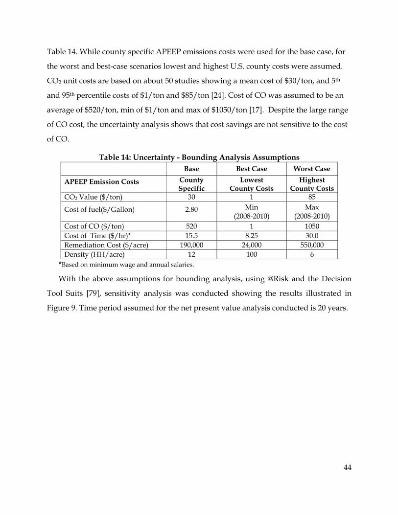
44

Table 14. While county specific APEEP emissions costs were used for the base case, for

the worst and best-case scenarios lowest and highest U.S. county costs were assumed.

CO2 unit costs are based on about 50 studies showing a mean cost of $30/ton, and 5th

and 95th percentile costs of $1/ton and $85/ton [24]. Cost of CO was assumed to be an

average of $520/ton, min of $1/ton and max of $1050/ton [17]. Despite the large range

of CO cost, the uncertainty analysis shows that cost savings are not sensitive to the cost

of CO.

Table 14: Uncertainty - Bounding Analysis Assumptions Base Best Case Worst Case

APEEP Emission Costs County Specific

Lowest County Costs

Highest County Costs

CO2 Value ($/ton) 30 1 85

Cost of fuel($/Gallon) 2.80 Min (2008-2010)

Max (2008-2010)

Cost of CO ($/ton) 520 1 1050 Cost of Time ($/hr)* 15.5 8.25 30.0 Remediation Cost ($/acre) 190,000 24,000 550,000 Density (HH/acre) 12 100 6

*Based on minimum wage and annual salaries.

With the above assumptions for bounding analysis, using @Risk and the Decision

Tool Suits [79], sensitivity analysis was conducted showing the results illustrated in

Figure 9. Time period assumed for the net present value analysis conducted is 20 years.

Figure

Sens

towards

Furth

brownfi

rate, usi

(100HH

lowest c

and low

cost savi

this anal

$1,300 re

10 illustr

e 9: Sensitiv

itivity analy

s the remed

hermore, th

elds ranges

ng the lowe

/acre), it w

cost saving

west density

ings even w

lysis). The h

equire a de

rates these

vity Analys

ysis results

diation cost

he results sh

s from $1,30

est remedia

will only tak

of $1,300), w

y (6HH/acr

with the lar

highest rem

nsity of 55

comparison

sis Results Dev

s shown ind

of brownfie

how that th

00 to $5,700

ation cost ($

ke 1 year to

while with

e), the reme

gest cost sa

mediation co

units per ac

ns for a 20 y

for Total Cvelopments

dicate that t

elds follow

he total cost

0 per house

$24,000/acr

offset the c

the highest

ediation co

aving of $5,

ost of $550,

cre to make

year time p

Costs (Costs

the cost sav

wed by the v

t savings of

ehold. Assu

re) and the

cost of reme

t remediati

ost is never

700 (given

,000 and the

e up for the

period.

t Savings) o

vings are m

value of tim

f driving as

uming a 7 p

highest den

ediation (ev

ion cost ($5

covered by

the assump

e lowest co

e cost in 10

of Brownfie

most sensitiv

me assumed

ssociated w

ercent disco

nsity

ven with th

50,000/acre

y the annua

ptions mad

ost saving o

years. Figu

45

eld

ve

d.

ith

ount

he

e)

al

de in

f

ure

Figuree 10: Net Pr(Com

resent Valumparison of

ue Analysisf Remediati

s for the Baion Cost an

ase, Best annd Other C

nd Worst CCost Saving

ase Scenarigs)

46

ios

47

3.2.9 Comparison of VMT and GHG Emission Reductions

Although methods to estimate VMT and GHG reduction are different between this study

and some previous studies (i.e. TAZ level data vs. Census level data; valuation and

accounting vs. life cycle assessments), the existing literature provides an opportunity to

compare and validate the results of this study. Relevant existing reported VMT

reductions are shown in Table 15:

Table 15: Comparison of VMT and GHG Reductions between Various Studies

Study Geographic Area Type of

Land-Use

Average Reduction

in VMT

Range of Reduction

in VMT

Range of Reduction in GHG & Air Pollutants

This Study Baltimore, Pittsburgh, Chicago, Minneapolis

Brownfield 52% 38% - 63% 35%- 75%

[51] Seattle, Minneapolis, St. Paul, Emeryville, Baltimore, Dallas

Brownfield 47% 32% - 57% 32% - 57%

[80-85]

12 cities: Atlanta, Baltimore, Boston, Charlotte, Denver, Dallas, Nashville, Sacramento, San Diego, Montgomery, West Palm Beach, BCD

Brownfield 61% 39% - 81% -

[49] Baltimore and Dallas Brownfield - 23% - 55% 36%-87%*

[50] Atlantic Station, Atlanta Brownfield 73%** 14%-52% -

[78] U.S. Compact 40% 20%-60% 20%-60%

[24] U.S. Compact - 5%-25% 5%-25%

[40] U.S. Compact 30% 20%-40% 18%-36%

[52] Minneapolis, Baltimore, Chicago, St. Louis, Pittsburgh, Milwaukee,

Brownfield *** *** 36%

*Actual number reported is 73 percent. The range was from pre-development model. ** The range is only showing the reduction of VOC and NOx. *** Nagengast does not directly calculate VMT, but rather focuses on travel time and concludes that travel time for brownfields is only 3 minutes less than greenfields.

The variation observed in the estimates reported by various studies can be the result

of many factors including method used, trip generation assumptions in different

jurisdictions, vehicle emission profiles varying in different geographical boundaries,

and uncertainties in estimating externalities. While these uncertainties and

inconsistencies are inevitable, the literature results show a 43±38 percent reduction for

48

VMT, which is consistent with the results of this study (38-63 percent). Furthermore, the

literature results show a 46±41 percent emissions reduction, which is consistent with the

results of this study (35-75 percent).

Travel times associated with brownfield sites are further compared to the national

averages and census journey to work data in Table 16 [1, 77].

Table 16: Brownfield Sites' Travel Time Comparisons with the National Averages Home-Based

Work (min) Home-Based

Non-Work (min) This Study 12 19

NHTS 2009 (National Average) [86] 24 18

Census 2000 (National Average) [87] 26 -

While the travel time estimates for HBNW trips used in this study are very similar to

the National Household Travel Survey (NHTS) average [86], the HBW travel time is

half of the other estimates, likely due to the close proximity of the small sample size to

work and city centers. This difference implies that characteristics of brownfield

developments (i.e. location) should be considered as they can impact travel patterns.

The following section examines some of these characteristics.

3.2.10 Brownfield Developments Characteristics and VMT Reductions

As mentioned in Section 3.2, most urban brownfields are developed as mixed-use or

compact developments. Compact development characteristics such as density,

diversity, design and distance to city centers may all be affecting the reduction in VMT,

number of trips and distance per trip. To examine if these characteristics are correlated

with the reduction in VMT, using all 16 sites studied in this analysis and despite of the

small sample size, a number of characteristics associated with compact developments

were explored. The result of the correlation analysis shows that as distance to the city

center increases, VMT increases; as access to transit improves, VMT decreases; and as

walkability improves, VMT decreases. Furthermore, brownfield developments show

wider and higher range of density associated with less VMT, while greenfield

49

developments show less dense developments (less than 3 households/acre) with higher

VMTs.

In detail the density of each site was calculated as a number of households per acre.

The distances between the site and the city centers were measured using shortest

driving distance. Access to transit was measured in terms of minutes to the city centers

using transit. Walkability was measured on a scale of zero to one hundred depending

on the number of amenities within one mile of the site [88].

The strongest correlation exists between VMT and distance to the city center,

indicating as distance increases, VMT increases (HBW = 0.80; HBNW = 0.73 ). Access to

transit (HBW = 0.78) shows as transit time increases, HBW trips also increase (not as

strong for HBNW trips, HBNW = 0.5), and walkability showing as the power of

walkability increases, VMT decreases (HBW = -0.64, HBNW = - 0.4). Compared with

other factors, density shows a weak correlation with HBW trips (HBW = -0.5) and almost

no correlation with HBNW trips (HBW = -0.02). Figure 11 shows that, in general,

greenfield developments have lower density (typically below 3 households per acre)

and higher VMTs while brownfield developments have higher densities with wider

range and fewer VMTs.

Figure 11: Home Based Work (HBW) Daily VMT vs. Density

0.00

5.00

10.00

15.00

20.00

25.00

30.00

0.1 1.0 10.0 100.0

Home Based W

ork Daily VMT (m

iles)

Development Density (HH/Acre)

VMT HBW BF

VMT HBW GF

Mean

50

3.2.11 Brownfield Developments and Other Social and Economic Factors

Although time, fuel and environmental cost savings of brownfield developments are

important factors when it comes to making decisions to move to urban areas, vacancy

rates of the 16 study developments show the average vacancy rate of brownfield

developments is higher (9 percent) than greenfield developments (1 percent). The

difference is statistically significant with 95 percent confidence (p=0.002). Vacancy rates

were estimated from the 2010 United States Postal Services data on houses that have

been vacant in the 90 days prior to this analysis [89]. So the question is if moving to

brownfield developments would save about 60 percent on the cost of fuel and time,

why is the vacancy rate higher in urban cores? Economic and social factors such as

home value, property taxes, crime rate and quality of schools are known to be among

the most significant factors influencing vacancy rates. Although the focus of this

analysis is not on the social aspects of brownfield developments, a few of these factors

were briefly studied for the 16 study developments to examine what might influence

people’s decisions.

To examine if the home value or the property tax is affecting vacancy rates, the 2009

median home values and property taxes were examined. The average home value of the

brownfield developments is about $220,000 while the average home value of the

greenfield developments is about $290,000 [90] (same characteristics). Home values

might be simply higher in or around greenfield developments as properties generally

have more land resulting in a higher price. The 2009 property tax data for the 16 sites

show that the average property tax of brownfield developments is 1.4 percent while the

average property tax of greenfield developments is about 1.3 percent [90]. While I

recognize that the sample size is small, examining the average home values and

property taxes, it was concluded that for the 16 study sites examined in this chapter,

property tax and home values are not the major determining factors. Other factors such

as crime rate or quality of schools may affect people’s decision more significantly.

51

3.3 Reducing Demand: VMT Reduction and Smart Growth Principles

In addition to land use strategies (i.e. brownfield developments assessed in the previous

section), there are other VMT reduction strategies that can have significant impact on

reducing travel activity. These strategies include but are not limited to parking

strategies, alternative modes strategies (i.e. biking, walking, public transit),

telecommuting, and pricing strategies. The 2010 DOT report released to the U.S.

Congress [8] examined five major categories of VMT reduction strategies: 1) pricing 2)

transit, non-motorized and intermodal travel 3) land use and parking 4) commute travel

reduction and 5) public information campaign. Each of these strategies was assessed in

isolation. In this section I examine the marginal impact of a number of these VMT

reduction strategies (i.e. biking and walking improvements, parking pricing, etc.) if they

are implemented as part of a land use development. The objective is to assess the

impact of each additional demand reduction measure, if it is implemented as part of a

land use strategy such as an infill or a brownfield development. This section builds

upon the previous section (3.2) analyzing travel patterns of sixteen residential

brownfield and conventional developments in the U.S. The additional VMT reduction

strategies being analyzed are known as smart growth principles that are part of the

LEED certification building standards.

3.3.1 VMT Reduction Measures and LEED

With the Leadership in Energy and Environmental Design (LEED) certification system

developed by the United States Green Building Council (USGBC) gaining rapid

popularity and recognition over the past decade, brownfields redeveloped in

combination with achieving the LEED travel reduction credits (those credits reducing

VMT) can help achieve VMT and GHG reduction goals effectively and at a faster rate.

By developing brownfields or any type of infill site, traffic becomes more concentrated

in the urban core as people occupy these developments. Therefore traffic congestion

will increase as a result of the shift of population from suburb to urban areas. In order

52

to balance the need for driving induced by the shifted population, smart growth

principles that reduce VMT such as those categorized under LEED standards as

transportation credits should be deployed.

The types of buildings included in a brownfield development are design decisions

on the part of constructors and owners. These design decisions can choose energy

efficient buildings but also include features that can further reduce VMT. Since

brownfield development VMT reductions estimated in section 3.2 are for residential

developments only, in this section we consider travel reduction credits in the LEED new

residential development (LEED® for Homes) and LEEDTM for Neighborhood

Development (ND) standards. The goal is to gauge the additive impact of VMT

reduction LEED credits, when they are incorporated into the design of brownfield

developments.

USGBC LEED certification is the most popular green building standard in the US.

The certification is obtained by amassing a prescribed number of credits for each new

development, with different levels of certification corresponding to different levels of

credits obtained. In the LEED® for Homes Rating System report [91], there are two

sections providing points that could potentially reduce VMT: 1) Sustainable Site (SS)

and 2) Location and Linkages (LL).

Under the SS section, SS 6 category called “compact development” provides a

minimum of 2 and a maximum of 4 points (moderate, high and very high density)

while potentially reducing VMT. The objective of SS 6 category is to preserve land while

increasing transportation efficiency and walkability. Multi housing units with average

density of 7 to 20 or more residential units can earn LEED points under this category

[91].

Under the LL section of LEED® for Homes, six measures shown in Figure 1 can

provide a maximum of 10 LEED points. If LL1 is satisfied, LL2-6 cannot be used and

vice versa.

To ea

Neighbo

minimu

points p

acquired

In th

maximu

case LL5

LL5:

maximu

-

-

-

In su

have up

F

arn LL poin

orhood Dev

m of 40 poi

possible und

d.

he case that

um of 10 po

5 is the only

Communit

um of 3 poin

Select a s

resource

Or select

resource

Or select

to 125 tra

ummary a L

p to seven V

Figure 12: L

nts under L

velopment

ints out of 1

der LEED N

a residentia

ints from L

y measure t

ty Resource

nts [91].

site that is l

s such as ba

t a site that

s.

t a site that

ansit rides p

LEED certifi

VMT reduct

Location an

LL1, the dev

(ND) [92]. A

110 points p

ND a maxim

al brownfie

LL2 to LL6 c

that can pot

es/Transit w

ocated with

anks, dayca

is located w

is located w

per weekda

ied multiun

tion points u

nd LinkagesS

velopment s

A neighbor

possible to

mum of 41 V

eld redevelo

categories (

tentially re

with an obj

hin ¼ a mil

are centers,

within ½ a m

within ½ a m

ay (bus, rail

nit resident

under LEED

s Category System [75]

should be c

rhood deve

be certified

VMT reduc

opment is n

(Figure 12)

sult in VMT

jective of pr

le of 4 to 11

, school, res

mile of 7 to

mile of tran

l and ferry

tial brownfi

D® for Hom

under LEE

certified as

elopment sh

d as LEED N

ction points

not LEED N

can be cred

T reduction

romoting le

basic comm

staurants, e

o 14 basic co

nsit services

combined)

ield develo

mes SS6 and

ED for Hom

LEEDTM fo

hould earn

ND. Of the

s can be

ND certified

dited. In tha

n:

ess VMT fo

munity

etc.

ommunity

s that offer

opment can

d LL5

mes Rating

53

or

a

110

d, a

at

or a

30

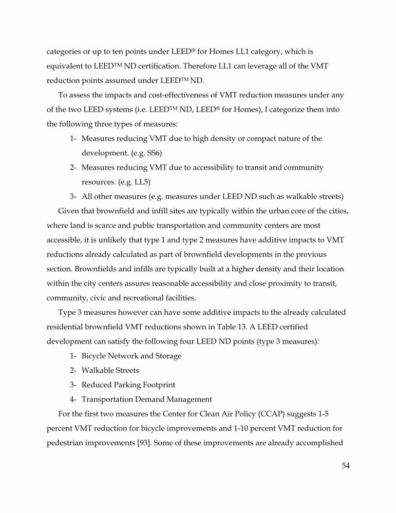
54

categories or up to ten points under LEED® for Homes LL1 category, which is

equivalent to LEEDTM ND certification. Therefore LL1 can leverage all of the VMT

reduction points assumed under LEEDTM ND.

To assess the impacts and cost-effectiveness of VMT reduction measures under any

of the two LEED systems (i.e. LEEDTM ND, LEED® for Homes), I categorize them into

the following three types of measures:

1- Measures reducing VMT due to high density or compact nature of the

development. (e.g. SS6)

2- Measures reducing VMT due to accessibility to transit and community

resources. (e.g. LL5)

3- All other measures (e.g. measures under LEED ND such as walkable streets)

Given that brownfield and infill sites are typically within the urban core of the cities,

where land is scarce and public transportation and community centers are most

accessible, it is unlikely that type 1 and type 2 measures have additive impacts to VMT

reductions already calculated as part of brownfield developments in the previous

section. Brownfields and infills are typically built at a higher density and their location

within the city centers assures reasonable accessibility and close proximity to transit,

community, civic and recreational facilities.

Type 3 measures however can have some additive impacts to the already calculated

residential brownfield VMT reductions shown in Table 13. A LEED certified

development can satisfy the following four LEED ND points (type 3 measures):

1- Bicycle Network and Storage

2- Walkable Streets

3- Reduced Parking Footprint

4- Transportation Demand Management

For the first two measures the Center for Clean Air Policy (CCAP) suggests 1-5

percent VMT reduction for bicycle improvements and 1-10 percent VMT reduction for

pedestrian improvements [93]. Some of these improvements are already accomplished

55

through the compact and mixed-use nature of brownfield or infill developments, since

residents of brownfields or infill have better accessibility to various facilities and live in

close proximity of them. However, design factors such as providing connectivity

through building sidewalks and bike paths, illumination of streets, sidewalks and bike

paths as well as providing scenery and shade can be incorporated within the

developments to further encourage biking and walking. Although separating the

impacts of the design factors from the effects of mixed use and high density

developments is not an easy task, there is some literature attempting to do so. A study

of fifty developments done by Cervero [94] found that each doubling of connectivity

design factor reduced VMT by 3 percent. LUTAQ [95] analyzed VMT in Puget Sound

area finding that residents living in communities with the most interconnected street

networks drive 26 percent less. Boarnet [96] found that pedestrian environmental

factors have a significant impact on increasing non-work travel at the neighborhood

level. Case studies in Davis, California and Boulder, Colorado further show that

providing bike networks and walkable streets can decrease driving from 1 to 10 percent

[93]. Summarizing what was found in the literature, given that reduction of VMT due to

the compact and high density nature of brownfields is already incorporated into the

brownfield VMT reduction calculations in Table 13, I assume 1 to 5 percent of additive

VMT reduction impact due to pedestrian and bicycle design factors.

CCAP suggests the VMT reduction from reduced parking footprint of 5 to 25

percent. These parking management programs could include car sharing programs,

unbundling of parking and rent prices, providing transit passes, incorporating

maximum parking limits, providing cash out incentives to employers, and others. Most

of these programs (e.g. cash out incentives) are more feasible for retail and commercial

developments. For residential developments, providing car sharing programs and

unbundling of pricing seem to be most feasible. Based on the literature, VMT reduction

from car sharing varies significantly and no study on impacts of unbundling could be

found. Steininger [97] suggests that car sharing reduces urban VMT by 2.7 percent.

56

Shaheen [98] reported VMT reduction of 37 percent and 58 percent in Netherlands and

Germany respectively due to car sharing. Copper [99] shows 7.6 percent VMT reduction

with the use of car sharing programs. Litman [100] and Lane [101] forecasted that the

impact of car sharing would be a reduction of privately owned vehicles by 6 to 12

percent. Cervero [102] assumes that car share users would reduce their VMT by 25

percent. Based on the literature review, for the residential brownfield development I

use a market share of 20 percent [98] meaning that 20 percent of residents enroll in a car

share program and the range of 7 to 12 percent for VMT reduction of those enrolled.

Under Transportation Demand Management LEED point the following five options

are possible (One point for every two options for a maximum of two points [92]):

Table 17: LEED Transportation Demand Management Options

Options Description Feasibility

TDM Program Create a program that reduces weekday peak period VMT by at least 20%.

Very Low

Transit Passes Provide transit passes for at least a year, subsidized to be half of regular price or cheaper.

Low

Developer Sponsored Transit

Provide year-round, developer sponsored private transit service from at least one central point in the project to other major transit facilities.

Low

Vehicle Sharing Locate the project such that 50% of the dwelling units entrances are within one quarter of a mile walk distance of at least one car sharing program.

Moderate to High

Unbundling of Parking

To sell or rent parking spaces separately from the dwelling units.

Moderate to High

In Table 17 under the third column the following rationale was used to rate the

feasibility of each option: In a residential brownfield development that is already

reducing VMT due of its compact and high density characteristics, the feasibility of

creating other TDM programs that could reduce VMT by an additional 20 percent is

very low. This is also due to the fact that LEEDTM ND states [92], “Any trip reduction

effects of Options 2, 3, 4, or 5 may not be included in calculating the 20 percent

57

threshold.” Providing transit passes and developer sponsored transit services not

common within residential developments are practiced more often within mixed use

developments with commercial and retail components. The additive impact of vehicle

sharing and unbundling parking although more feasible to implement is already

calculated as part of the “reduced parking footprint” category. Therefore, no additional

impacts were considered under the “vehicle sharing” and “unbundling of parking”

categories. In other words, the maximum potential VMT reduction impacts from either

of these categories were already assumed under the “reduced parking footprint”

category.

In summary the additive VMT reduction impacts of implementing LEED points

ranges between 1 to 12 percent for reducing VMT through bike paths, walkable streets,

unbundled parking and car sharing programs. To benefit from these VMT reduction

percentages and to credit LEED points associated with these reductions, owners and

developers need to incorporate these measures in the design and planning of any

brownfield development project. Two important factors should be considered while

conducting benefit and cost analysis of LEED certified buildings:

1) The probability of achieving VMT reduction through LEED points decreases as

percent VMT reduction goes up. In other words there is a higher chance of achieving 1

percent VMT reduction through LEED points than achieving 12 percent VMT reduction

through LEED points.

2) In some cases although LEED measures are implemented and a building is LEED

certified, energy savings and GHG emission reductions may actually not be achieved

[103]. The same may occur for VMT reductions.

On the cost side, a LEED certified development incurs a higher cost of construction

compared with a conventional development plus an additional soft cost of

documentation, review fees and commissioning. USGBC [104] report looked at 110

projects in New York City of which 63 were LEED certified. Results show that on

average LEED certified high-rise residential buildings on average cost $175,000 per acre

58

more than non-LEED buildings [104]. According to Kats [105], green buildings cost

about 2 percent more to construct than conventional buildings. Kats reports that the

construction cost of green buildings is $3-$5/ft2 higher than conventional buildings

(approximately $130,000 to $220,000 per acre). An older study, Northridge

Environmental Management Consultants (NEMC) [106] , reports LEED certification

adds 4 to 7 percent to a project’s construction cost. In addition NEMC [106] reports the

cost of documentation as low as $10,000 and as high as $60,000 per project. For the cost

side of this analysis I use an average value of $175,000 per acre assuming our residential

brownfield redevelopment is LEED certified [92]. Higher ratings of LEED certification

(i.e. Silver, Gold) would probably increase the cost of construction. However this study

analyzes costs and benefits of minimum required points for certification only. To

qualify for compact developments under LEED, density should be between 7 to 21

dwelling units per acre. I assume an average density of 15 dwelling units per acre, and 5

percent discount rate for 30 years.

Adding percent reductions to the VMT that was already reduced by moving from a

conventional development to a brownfield development (Table 13), and updating cost

data so that it includes the cost of remediation and LEED certification, the following

cumulative annual cost savings can be expected.

Table 18: Per Household and per Capita Annual Cost Saving Ranges of Brownfield Redevelopments when Combined with VMT Reducing LEED Points

Annual Cost/Savings $/household $/person

Cost of Fuel Saved 430-460 180-190

Cost of Time Saved 1,940-2,080 800-870

Cost of Maintenance Saved 280-300 120-125

Total Direct Savings 2,650-2,850 1,100-1,200

External Environmental Costs Saved 450-480 190-200

Total Savings 3,100-3,300 1,300-1,400

Remediation + LEED (1500) (600)

Net Savings 1,600-1,800 700-800

59

Table 18 shows that when a brownfield site is developed as a residential multiunit

development, incorporating and implementing LEED VMT reduction measures -

including bicycle network and storage, walkable streets, unbundling and car sharing

programs – can potentially save each household up to an extra $200 and each person up

to an extra $100 a year on the direct costs (time, fuel and maintenance). However since

cost of LEED certification adds about 70 percent to the original cost of brownfield

remediation, the net savings are less in the case of LEED brownfield developments

compared with non-LEED brownfield developments. Percent VMT reduction from

LEED points need to increase to 30 percent in order for the net savings to be the same as

non-LEED brownfield developments (Table 13).

As mentioned previously, this chapter only includes residential developments.

Therefore only LEED points that pertain to residential developments were included in

the analysis. Brownfield developments often have commercial and retail components to

them. In case that a commercial brownfield development is being analyzed, LEED for

New Construction (LEED NC) points are more favorable to be used for the analysis.

LEED NC includes the following three potential VMT reduction measures [107]:

1- Alternative Transportation: Public Transportation Access

2- Alternative Transportation: Bicycle Storage and Changing Rooms

3- Alternative Transportation: Parking Capacity

Of these three measures, public transportation access (as mentioned previously) will

not have much of an additive impact since brownfields are already located in urban

cores with a better access to transit. The next two measures, bicycle storage and

changing rooms as well as parking capacity, are common in all LEED standards and

have already been accounted for in the analysis of brownfield residential developments.

Therefore, if commercial components are added to brownfield residential

developments, I do not anticipate a significant cost saving from any additional LEED

VMT reduction measure generated by the residents of the brownfield development.

Non-brownfield residents may generate some travel savings by using the facilities

60

provided as part of the commercial brownfield developments. This study does not

include the VMT cost savings generated by non-brownfield residents.

3.4 LEED Certified Brownfield Developments Vs. Other VMT Reduction Measures

In recent years a number of studies have been conducted to quantify benefits and costs

of various VMT reduction strategies [40, 78, 93, 108]. The U.S. DOT [8] report to the U.S.

Congress combines results of many of these studies to show how various VMT

reduction strategies can be environmentally effective. To compare brownfield

redevelopments and LEED certified brownfield redevelopments with other travel

reduction strategies, the same definitions and assumptions as DOT [8] were used to

generate the cost-effectiveness estimates for this part of the analysis: for direct

implementation cost, remediation cost and the cost of LEED certification are considered.

For the net benefit, direct implementation costs as well as cost savings from fuel use,

externalities and vehicle operation were included. For consistency between this analysis

and the DOT report, all direct costs are reported in 2010 year real dollars (when both

studies were done: this study and the DOT study [8] without any inflation or

discounting. For calculating net benefits, however, future year operating cost savings

were discounted using the rate of 7 percent. Results are shown in Table 19.

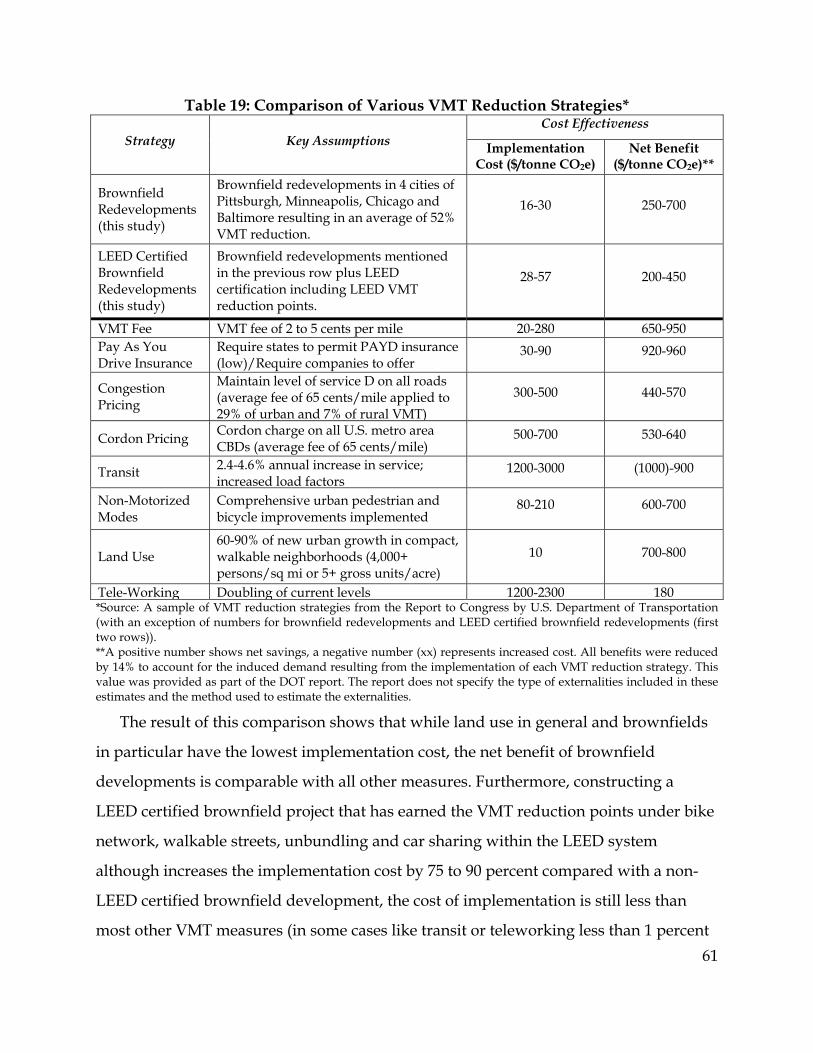
61

Table 19: Comparison of Various VMT Reduction Strategies*

Strategy Key Assumptions Cost Effectiveness

Implementation Cost ($/tonne CO2e)

Net Benefit ($/tonne CO2e)**

Brownfield Redevelopments (this study)

Brownfield redevelopments in 4 cities of Pittsburgh, Minneapolis, Chicago and Baltimore resulting in an average of 52% VMT reduction.

16-30 250-700

LEED Certified Brownfield Redevelopments (this study)

Brownfield redevelopments mentioned in the previous row plus LEED certification including LEED VMT reduction points.

28-57 200-450

VMT Fee VMT fee of 2 to 5 cents per mile 20-280 650-950 Pay As You Drive Insurance

Require states to permit PAYD insurance (low)/Require companies to offer

30-90 920-960

Congestion Pricing

Maintain level of service D on all roads (average fee of 65 cents/mile applied to 29% of urban and 7% of rural VMT)

300-500 440-570

Cordon Pricing Cordon charge on all U.S. metro area CBDs (average fee of 65 cents/mile)

500-700 530-640

Transit 2.4-4.6% annual increase in service; increased load factors

1200-3000 (1000)-900

Non-Motorized Modes

Comprehensive urban pedestrian and bicycle improvements implemented

80-210 600-700

Land Use 60-90% of new urban growth in compact, walkable neighborhoods (4,000+ persons/sq mi or 5+ gross units/acre)

10 700-800

Tele-Working Doubling of current levels 1200-2300 180 *Source: A sample of VMT reduction strategies from the Report to Congress by U.S. Department of Transportation (with an exception of numbers for brownfield redevelopments and LEED certified brownfield redevelopments (first two rows)). **A positive number shows net savings, a negative number (xx) represents increased cost. All benefits were reduced by 14% to account for the induced demand resulting from the implementation of each VMT reduction strategy. This value was provided as part of the DOT report. The report does not specify the type of externalities included in these estimates and the method used to estimate the externalities.

The result of this comparison shows that while land use in general and brownfields

in particular have the lowest implementation cost, the net benefit of brownfield

developments is comparable with all other measures. Furthermore, constructing a

LEED certified brownfield project that has earned the VMT reduction points under bike

network, walkable streets, unbundling and car sharing within the LEED system

although increases the implementation cost by 75 to 90 percent compared with a non-

LEED certified brownfield development, the cost of implementation is still less than

most other VMT measures (in some cases like transit or teleworking less than 1 percent

62

of the cost). This result further shows the net benefit of LEED certified brownfield

redevelopments are comparable with some of the other VMT measures. Therefore it is

apparent that residential brownfields and residential LEED certified brownfields could

serve as a viable strategy to reduce travel activity and the associated environmental

impacts.

3.5 Discussion

From the governmental standpoint, especially state and local transportation authorities,

brownfield developments and in particular LEED certified brownfield developments

can serve as a cost-effective VMT reduction strategy. Table 20 shows some of the

potential costs and benefits that brownfield development stakeholders might incur.

Table 20: Stakeholders' Benefits and Costs of Brownfield Developments

Who? Potential Benefits Potential Costs

Local Residents Reduced Health Risks – Increased Home Values– Reduced Crime Rate

Increased Tax – Noise Congestion

Brownfield Residents

Saved Time – Saved Fuel Improved Health

Safety Concerns Lower Quality of School

Developers Existing Infrastructure - Zoning Differentiation - Funds and Subsidies

Remediation Cost - Timing Issues Liability Concerns

Society at Large

Improved Health Reduced Emission

Tax

The City Property Tax – Employment Opportunities – Other Income

Negligible

Government Achieving Emission Reduction Goals Various Fees

Funding - Subsidies

Transportation Authorities

Achieving VMT Reduction Goals – Increasing Cost Effectiveness of

Transit

Negligible

Most stakeholders incur some type of a cost when it comes to brownfield and LEED

Brownfield redevelopments. However transportation authorities have a minimal cost

since most of the cost of brownfield developments and LEED certification are either

63

paid by a developer or environmental agencies such as the U.S. EPA, which provides

funding and incentives for the initial remediation cost of the sites. Therefore, results of

this benefit cost analysis should encourage metropolitan planning organizations and

state and local transportation governments as well as the transportation policy makers

to consider brownfield redevelopments and especially LEED certified brownfield

redevelopments as a VMT reduction strategy by encouraging and providing additional

funding and incentives to other brownfield stakeholders. Furthermore, transportation

authorities should join efforts with the U.S. EPA to identify and provide incentives that

would result in an increased modal shift, such as those that are in close proximity of

transit infrastructures and services. In cooperation with the cities and planning

departments, transportation authorities can also provide incentives and grants that

would encourage developers and planners to implement smart growth principles such

as diversity and interconnectivity.

The strategies discussed here could also be augmented with additional measures to

further reduce vehicle miles traveled and greenhouse gas emissions. For example,

mixed use developments could further reduce overall travel demand. Energy efficient

buildings could reduce GHG for heating, ventilation and cooling [103].

3.6 Commercial and Retail Brownfields

Up to this section of this chapter the estimates related to brownfield developments and

LEED certified brownfield developments only included residential developments. In

this section I discuss retail brownfields and their impact on driving. A case study of

four retail brownfield sites in Allegheny County, Pennsylvania is assessed to evaluate

VMT savings generated from the development of these retail sites. The objective is to

provide guidance on how the location of a future retail store can potentially minimize

environmental damages associated with home based shopping driving.

With over 1.2 million people and an area of 730 square miles (1890 km2), Allegheny

County is home to Pittsburgh, the second largest city in the U.S. commonwealth of

Pennsylvania [109]. Reasons for the selection of this particular region to assess home

64

based shopping travel time savings are as follows: 1) availability of traffic analysis zone

(TAZ) data for the county, 2) its large potential for urban brownfield and infill

developments, and 3) knowledge of local traffic patterns.

3.6.1 Method

This study includes only residential travel patterns and savings, meaning those trips

that are originated from home (home to shopping) and went back home after shopping.

It does not include trips that are generated from work to shopping, shopping to non-

home destination or from one shopping origin to another shopping destination. The

study estimates residential travel savings from the development of four retail

brownfield and/or infill sites in terms of time, fuel and external environmental costs.

The method used to estimate costs of time, fuel and external environmental costs are the

same as the method used thus far in this work. In short, VMTs, speed data, emission

factors from MOBILE6 and damage costs from APEEP are joined to evaluate the cost

savings associated with the four brownfield/infill retail sites. The retail sites selected for

this study are Target, REI, Costco and Giant Eagle. There is one brownfield or infill

location selected for each of these stores and VMT savings associated with each of these

stores in comparison with other branches of the stores are estimated. The selection

criteria for choosing these stores were to 1) retail stores that have a location categorized

as brownfield or infill within Allegheny County and 2) to cover a variety of stores that

customers would go to in varying frequencies (e.g. twice a week to Giant Eagle and

once a week to Target). Cost savings are estimated for an average household in

Allegheny County assuming that each household makes trips to all four store types (i.e.

REI, Costco, Giant Eagle and Target) annually. Figure 13 illustrates the location of

brownfield stores and other branches of the stores, in Alleghany County, that were

compared in this analysis.

To es

REI, all l

included

convent

Target a

branche

that thos

brownfi

location

between

calculate

the rout

routes w

from TA

Figure 1

stimate trav

locations w

d one brow

ional locati

and Giant E

s that are im

se locations

eld/infill lo

s are provid

n the centro

ed using sh

e with the s

were sugges

AZs and the

3: Location

vel savings,

within Alleg

wnfield locat

ions for Cos

Eagle, first t

mpacted by

s that consu

ocation wer

ded in App

oid of each T

hortest driv

shortest dri

sted by Goo

e two locati

n of Retail S

, first retail

gheny Coun

tion for Cos

stco and on

he infill/br

y the newly

umers woul

re selected.

pendix E. T

TAZ and al

ing distanc

iving distan

ogle. In case

ons (brown

Stores with

stores wer

nty were ide

stco, one br

ne conventio

rownfield lo

y developed

ld travel to

A complet

The second

ll selected r

ce provided

nce was cho

e of REI, th

nfield and c

hin Allegha

re identified

entified for

rownfield lo

onal locatio

ocation wa

d locations w

in the abse

te list of all

step was to

retail stores

d by Google

osen in case

he difference

conventiona

any County

d. In case of

r each store

ocation for

on for REI.

s identified

were select

ence of the

four stores

o calculate d

s. Distances

e [110]. For

es where m

e between t

al) would b

y, PA

f Costco an

e; These

REI, two

In case of

d. Then thos

ted. This me

new

s and their

distances

s were

consistency

multiple trav

the distance

be TAZ mile

65

nd

se

eans

y,

vel

e

e

66

saved, assuming the distance from the centroid of a TAZ to brownfield is less than the

conventional site. This method assumes that people always choose the closer location

for shopping. In case of Costco, Target and Giant Eagle, the method is the same while

the calculations are more complex as there are more competing locations. In case of

Target for instance, the site with the shortest distance among all conventional sites to

the centroid of a TAZ was selected. If the distance from the centroid of the TAZ to this

site was more than the distance from the centroid of the TAZ to the brownfield/infill

site, then the difference would be travel saved due to the existence of the new

brownfiled/infill site. The same method is used for Giant Eagle and Costco. The

following equations explain the method:

∑ , (4)

In cases where the TAZ centroid was either at an equal driving distance or further

from the site of interest than from an existing site (e.g. dEi ≤ dBi), there were no recorded

travel savings for that TAZ. The aforementioned equation results in TAZ mile savings

for each store for one directional trip, which means that there is only one household in

each TAZ and that is located in the center of the TAZ. To estimate the annual savings

due to the development of the brownfield/infill retail store SB is multiplied by the

number of households in each TAZ and the number of trips that each household takes

to each of the stores annually. To count for the roundtrip miles, assuming that

household travel to a store and return home, SB is also multiplied by 2.

Table 21 shows the assumptions used for the number of trips per household to each

store. These numbers are assumptions based on surveying a number of Pittsburgh

residents.

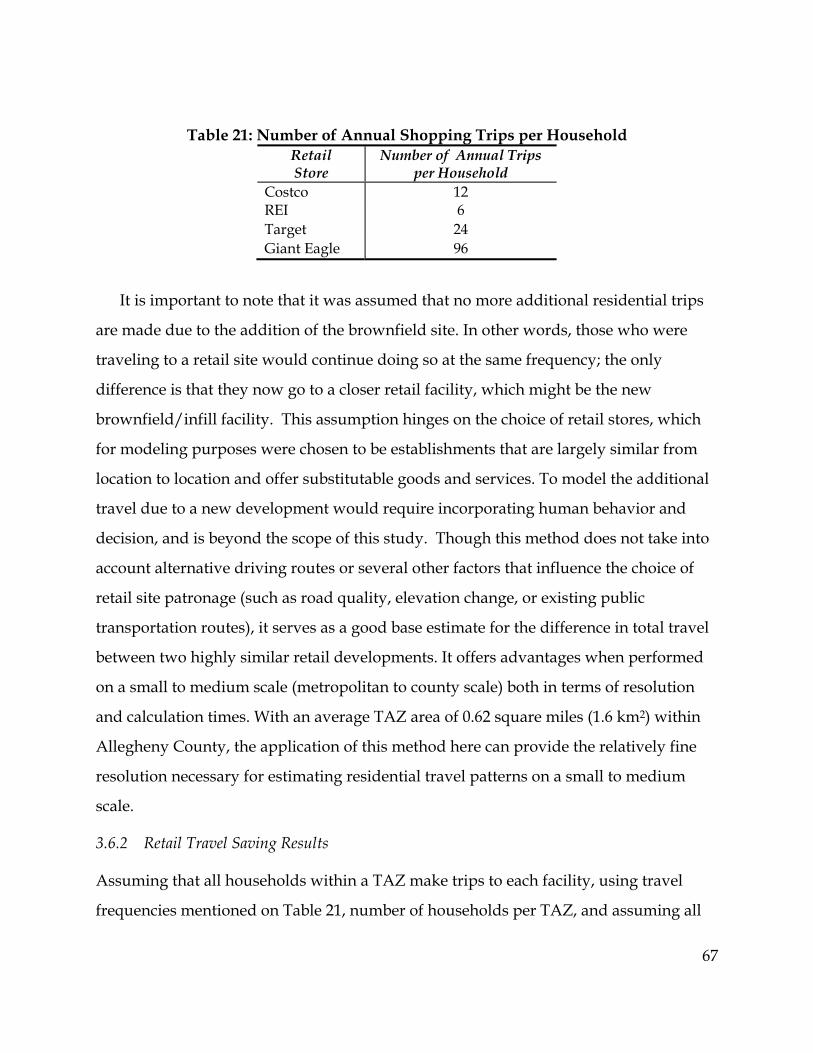
67

Table 21: Number of Annual Shopping Trips per Household Retail Store

Number of Annual Trips per Household

Costco 12 REI 6 Target 24 Giant Eagle 96

It is important to note that it was assumed that no more additional residential trips

are made due to the addition of the brownfield site. In other words, those who were

traveling to a retail site would continue doing so at the same frequency; the only

difference is that they now go to a closer retail facility, which might be the new

brownfield/infill facility. This assumption hinges on the choice of retail stores, which

for modeling purposes were chosen to be establishments that are largely similar from

location to location and offer substitutable goods and services. To model the additional

travel due to a new development would require incorporating human behavior and

decision, and is beyond the scope of this study. Though this method does not take into

account alternative driving routes or several other factors that influence the choice of

retail site patronage (such as road quality, elevation change, or existing public

transportation routes), it serves as a good base estimate for the difference in total travel

between two highly similar retail developments. It offers advantages when performed

on a small to medium scale (metropolitan to county scale) both in terms of resolution

and calculation times. With an average TAZ area of 0.62 square miles (1.6 km2) within

Allegheny County, the application of this method here can provide the relatively fine

resolution necessary for estimating residential travel patterns on a small to medium

scale.

3.6.2 Retail Travel Saving Results

Assuming that all households within a TAZ make trips to each facility, using travel

frequencies mentioned on Table 21, number of households per TAZ, and assuming all

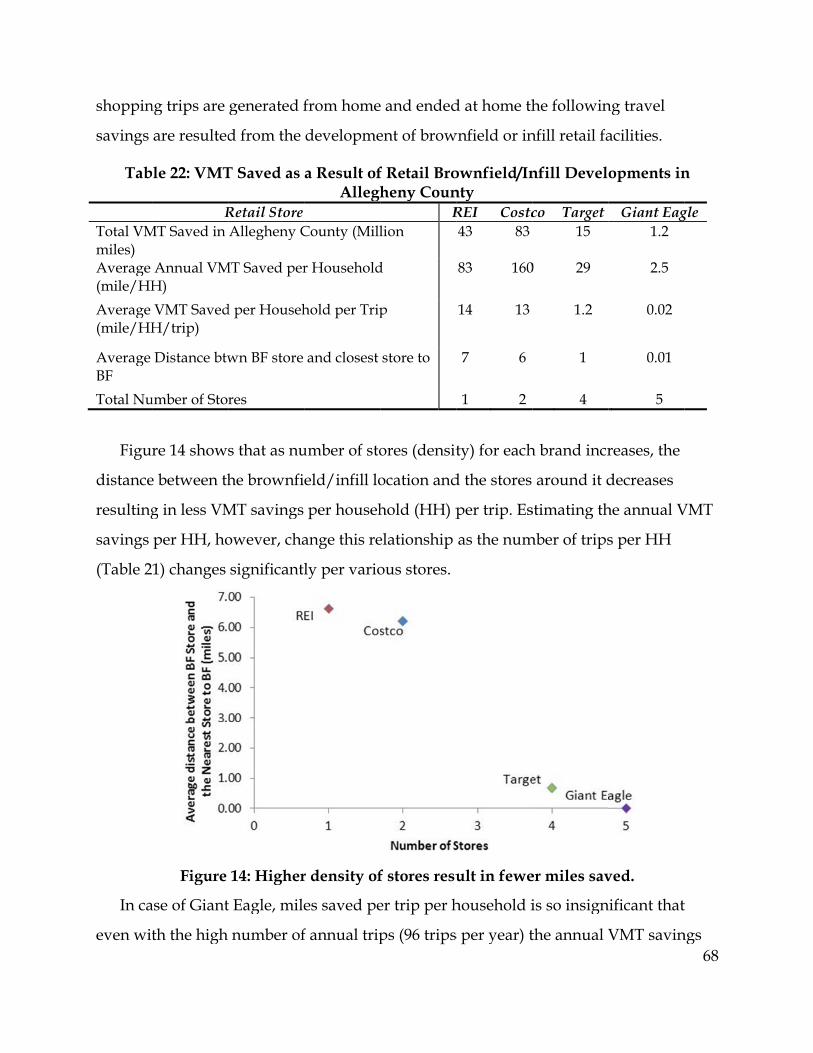
shoppin

savings

Tab

Total VMmiles) Average (mile/HH

Average (mile/HH

Average BF

Total Nu

Figu

distance

resulting

savings

(Table 2

In ca

even wit

ng trips are

are resulted

ble 22: VMT

RMT Saved in

Annual VMH)

VMT SavedH/trip)

Distance btw

umber of Sto

re 14 show

e between th

g in less VM

per HH, ho

1) changes

Figure

ase of Giant

th the high

generated f

d from the

T Saved as

Retail Store Allegheny C

MT Saved per

d per Househ

wn BF store

res

s that as nu

he brownfi

MT savings

owever, cha

significantl

14: Higher

t Eagle, mile

number of

from home

developme

a Result ofAllegh

County (Mill

r Household

hold per Trip

and closest

umber of sto

eld/infill lo

per househ

ange this re

ly per vario

r density of

es saved pe

f annual trip

e and ended

ent of brow

f Retail Broheny Coun

Rlion

d

p

store to

ores (densit

ocation and

hold (HH) p

elationship

ous stores.

f stores resu

er trip per h

ps (96 trips

d at home th

wnfield or in

ownfield/Innty REI Costc43 83

83 160

14 13

7 6

1 2

ty) for each

d the stores

per trip. Es

as the num

ult in fewe

household i

s per year) t

he followin

nfill retail fa

nfill Devel

co Target 15

0 29

1.2

1

4

h brand incr

around it d

stimating th

mber of trips

er miles sav

is so insign

the annual V

ng travel

acilities.

opments in

Giant Eag1.2

2.5

0.02

0.01

5

reases, the

decreases

he annual V

s per HH

ved.

nificant that

VMT savin68

n

gle

VMT

t

ngs

69

per household turns out to be about 1.5 percent of the annual VMT savings from

Costco. This VMT savings per HH resulted from development of an infill Target is

about 18 percent less than the VMT savings per HH resulted from Costco. This is all due

to the fact that the distance between the new brownfield/infill location and the second

best alternative to that location is short. In case of REI, where the VMT savings are

closer to that of Costco, since the number of trips per HH is significantly less than

Costco, the annual VMT savings per household are about 50 percent less. If annual REI

number of trips per household increases to once a month (same as Costco), the same

level of VMT savings are expected.

In summary, results shown above are dependent on a few factors. The most

deterministic factor is the density of retail stores (i.e. number of stores per square mile)

and the resulted proximity of the retail facilities to each other. In cases like Costco,

where there are only 2 conventional locations and they are far from the brownfield

Costco site, the VMT savings are larger. In the case of Giant Eagle where the closest

Giant Eagle to the Brownfield site is only 2 miles away, VMT savings are less. The

number of trips per household to each retail facility is also deterministic in the annual

VMT savings per household. This is apparent from the comparison of REI and Costco

annual travel savings.

This analysis provides a level of comparison between residential and retail

brownfield developments and the amount of VMT savings they each generate. As it

was discussed in the previous sections brownfield sites are typically located in urban

areas and are a subset of infill developments. While residential brownfield

developments result in about 60 percent VMT saving, retail brownfield developments

do not result in such significant savings in travel activity. The amount of VMT savings

expected from retail brownfield developments is highly dependent on the location of

the new site in comparison with the already existing retail stores. REI and Costco are

both good examples of effective planning of retail brownfield stores as each of the

brownfield locations result in significant VMT savings. The following Table shows the

70

direct and indirect cost savings generated from VMT savings of retail brownfield

developments.

Table 23: Average Annual Household Savings from Retail Brownfield Developments

Annual Cost/Savings $/household

Cost of Fuel Saved 26

Cost of Time Saved 150

Cost of Maintenance Saved 14

Total Direct Savings 190

External Environmental Costs Saved 30

Total Savings 220

Figure 15 breaks down the average annual external environmental cost savings of a

household for each pollutant. The external environmental cost savings are estimated

based on the APEEP model.

Figure 1

Com

followin

Table 2

A

Cost of Fu

Cost of Ti

Cost of M

Total Dir

External E

Total Sav

15: Average

mparing resi

ng results ar

24: Average

Annual Cost/S

uel Saved

ime Saved

Maintenance S

ect Savings

Environmenta

vings

e Annual Eto R

idential trav

re produced

e Annual CBrownf

Savings

Saved

al Costs Save

External EnRetail Brow

vel savings

d:

Cost Savingfield Devel

Residen$/h

ed

nvironmentwnfield by

with retail

g Comparislopments p

ntial Brownfieldhousehold

425

1,925

280

2,630

450

3,080

tal Cost Savy Pollutant

l travel savi

son betweeper Househ

d Retail B$/hou

2

1

1

1

3

2

vings per H

ings per ho

en Residenthold

Brownfield usehold

26

150

14

190

30

220

Household

ousehold, th

tial and Re

% Retail CSavings Comp

with Residen6

8

5

7

6

7

71

due

he

etail

Cost pared ntial

72

Results shown in Table 24 indicate that assuming each household travels to all four

retail facilities annually and according to the frequencies mentioned on Table 21, travel

cost savings from brownfield retail developments are in average 7 percent of those cost

savings resulted from living in a residential brownfield development.

73

“You are not stuck in a traffic jam. You are the traffic jam.”

-Advertisement in Germany

74

Chapter 4

Supply Congestion Management Strategies

4.1 Increasing Supply: Improving Traffic Operations

Congestion is typically caused by either too much demand or not having enough

supply. In addition to having insufficient lane capacity along a roadway, supply or

carrying capacity of roadways can be reduced by weather conditions, roadway

construction, and incidents. One obvious way of mitigating the lack of supply is to add

more infrastructure such as roads and bridges to the urban transportation network.

Because of the scarcity of land in urban areas, the significant cost of construction

associated with such infrastructure developments, and lack of funding, the option of

adding infrastructure is not feasible in most cases, especially in already well-developed

urban areas. Furthermore, experience has shown that increasing the number of roads or

lanes can result in increased traffic until the point of recurred congestion [111]. This

particular phenomenon, called induced demand, will be discussed in Chapter 5.

Another way to add supply to an existing roadway network is by implementing

operational strategies such as incident management strategies, traveler information

systems, work zone management, ramp metering, and adaptive signal control. These

operational measures and strategies can efficiently add more supply or compromise for

reduced supply and result in reduced congestion and consequential GHG emissions

[112]. Congestion management strategies have been debated extensively in the past,

though much of the work dates from the pre-information and communication

technology (ICT) era. Classic works describing the potential strategies and limitations

include Altshuler [14] on alternative policies and politics, Meyer [113] on urban form

and Wohl [114] on congestion pricing approaches and problems. Continuing concerns

about traffic congestion on the U.S. roads in the post-ICT era, have forced governments

to look beyond the conventional congestion management methods over the last two

decades. Alternatively, various applications of Intelligent Transportation Systems (ITS)

75

are now broadly recognized as tools to relieve traffic congestion. ITS applications

integrate information and communication technologies into transportation

infrastructure systems and vehicles to improve the efficiency and mobility of the surface

transportation system by increasing the carrying capacity [115].

In Chapter 3, I assessed demand management strategies including land use

strategies. Implementing land use strategies alone may reduce the GHG emissions

resulting from driving, but are unlikely to solve the problem of congestion. While land

use strategies in the form of compact mixed-use urban developments have the potential

to reduce VMT on a regional scale, they most likely add to the already existing

congestion locally by shifting the suburban population to the urban cores. Combining

land use strategies with ITS operational strategies may, however, effectively reduce

congestion and demand within urban areas and promote urban environmental

sustainability. While land use strategies such as brownfield developments may add

additional congestion to the already congested urban cores, implementing operational

strategies improves traffic flow and reduces congestion locally.

In this chapter, economic and environmental cost effectiveness of three congestion

management strategies that increase the existing supply and carrying capacity are

assessed. To estimate the cost effectiveness of these strategies, the same method

described in Section 2.3 was used. First, proactive monitoring of signal timing and

coordination is assessed, and economic and environmental costs and cost savings are

estimated. This assessment was done using a scenario-based analysis. Cost savings of

two other strategies - 1) high occupancy toll (HOT) lanes and 2) adaptive signal timing -

were estimated using values already reported in the literature.

4.2 Proactive Monitoring of Traffic Signal Timing and Coordination

To ensure that a traffic signal network is working efficiently level and traffic is

flowing safely and smoothly, regular monitoring of traffic demand and travel patterns

is necessary. Frequent evaluation of traffic volumes and signal timings followed by

updating of already implemented strategies and incorporating new strategies is critical

76

for rapidly growing cities and networks. The updates of implemented timing strategies

may include new timing plans, phasing, and offsets to better address the level of

demand. Timing plans, phasing, cycle lengths and offsets are essential for the operation

of traffic signals and signalized intersections. Definitions of the traffic signal timing

terminologies are provided in Appendix F.

Proactively monitoring and evaluating the operation of traffic signal systems and

strategies can be labor intensive. Because of budget constraints and labor shortages,

many jurisdictions are not able to operate their traffic signal systems to provide optimal

traffic flow and roadway capacity at all times, resulting in increased traffic congestion,

delays and emissions along their networks. Consequently, imperfect conditions along

arterial networks can increase some of the secondary negative impacts such as

accidents, noise and reduced safety.

This section estimates costs (direct and external environmental costs) associated

with traffic signal systems if they are not monitored, evaluated and maintained on a

regular basis for the level of vehicular and pedestrian demands. Implementing

traditional measures, such as signal timing optimization and coordination, to alleviate

the environmental problems can be cost effective if they are maintained and monitored

properly and operate efficiently [116]. While it seems intuitive that not updating traffic

signal timings on a regular basis would lead to a suboptimal level of network operation,

the results of this work illustrate that costs associated with the lack of frequent

evaluation of performance measures can be substantial. The objective is to encourage

jurisdictions and traffic operation teams to develop a system monitoring program to

allow each signalized intersection in their network to operate as efficiently as possible,

at all times. Traditional signal timing based on time of day (TOD) operation may only

be at an optimal level on the day that the timings were implemented and fine-tuned

since vehicular demand and travel patterns might change soon after the

implementation of the timings. Growth in population, fluctuations in volume, changes

in travel patterns, and developments in the area all can reduce the efficiency of the

77

implemented signal timings. The degree of such impact is clearly demonstrated in this

section using scenario-based analysis. The cost of fuel and time as well as the external

air pollution cost of not monitoring and updating signal timings are estimated for

signals along a traffic signal network in Cranberry Township, Pennsylvania.

4.2.1 Existing Traffic Signal Retiming Cost and Benefit Assessments

The benefits and measures of effectiveness of traffic signal retiming have been

quantified and evaluated in the literature, most of which focus on U.S. case studies.

Based on an analysis conducted on the Maryland Department of Transportation

retiming project of 215 signals in the Washington DC area, travel delay was decreased

by 13 percent and number of stops by 10 percent [117] by implementation of new

timings. The same paper lists more examples of successful signal retiming projects

including a Lexington, Kentucky retiming project that reduced delays by 40 percent; the

Traffic Light Synchronization Program in Texas reduced delays by 14 percent; and a

Jacksonville, Florida retiming project decreased travel time by 7 percent [117].

According to the Institute of Traffic Engineers [116], traffic signal retiming can result in

7-13 percent reduction in overall travel time, 15-37 percent reduction in overall traffic

delay, and 6-9 percent in overall fuel savings.

While many studies report on typical measures of effectiveness such as number of

stops, delay, speed, travel times and fuel consumption, only a few quantify benefits and

costs of signal retiming in terms of environmental impacts and user costs [118]. This

work examines cost savings of the traditional signal monitoring and retiming in terms

of time and fuel, environmental damages, mortality and morbidity.

4.2.2 Project Background

Cranberry Township, Pennsylvania is located at the crossroad of two interstate

highways, the Pennsylvania Turnpike (I-76) and I-79, twenty miles north of Pittsburgh

in neighboring Butler County. Its proximity to the major interstates as well as the city of

Pittsburgh has encouraged many businesses and corporations to move their

78

headquarters and offices into the Township resulting in major and rapid growth and

economic and social changes over the last decade.

To address this growth, Cranberry Township took an enormous step in improving

traffic operations by implementing new signal timings and updating their software and

hardware systems within the last two years (since 2010). The combination of a number

of factors including these newly implemented signal timing plans, and newly

implemented hardware and software traffic signal systems throughout the Township,

along with the geographic location of Cranberry Township and its rapid economic and

population growth, makes Cranberry Township a feasible case study to illustrate costs

associated with the lack of proactive monitoring of traffic signal retiming performance

measures.

Cranberry Township currently operates and maintains a total of 44 traffic signals, 37

within or partially within the Township limits, while the rest are in Adams and

Marshall Townships, as well as one in Seven Fields Borough in Butler County,

Pennsylvania. Two major corridors in Cranberry Township are Route 19 and Route 228.

Route 19 is significant to the traffic network systems as it runs parallel to the

Pennsylvania Turnpike (I-76) at the junction with I-79. Route 228 and Route 19 provide

access to both these interstates. Figure 16 illustrates the location of Cranberry Township,

its signalized intersections and the boundary of this analysis.

Fi

Duri

Operatio

signalize

currentl

of a cent

Townsh

Aries Cl

Detailed

To im

for all its

collected

igure 16: M

ing the Fall

on Center (

ed intersect

y installed

trally based

hip has a mi

losed Loop

d informatio

mprove ope

s signalized

d in 2009. A

Map of Cran

of 2010, Cr

TOC), curr

tions owne

at fifteen k

d system co

ix of NEMA

Operating

on on these

erations, Cr

d intersectio

All signalize

nberry Tow

ranberry To

ently respo

d and/or o

ey intersect

ommunicati

A TS2 Type

System, an

e hardware

ranberry To

ons in Apri

ed intersect

wnship Traf

ownship op

onsible for t

operated by

tions, and m

ing through

1 operation

nd Econolite

and firmw

ownship im

il of 2011, u

tions are cu

ffic Signal

pened a stat

the operatio

y the townsh

most signal

h a fiber op

n, Econolite

e’s Central

ware is prese

mplemented

using vehicu

urrently run

Zone, Sou

te-of-the-ar

on and mai

hip. Camer

lized inters

ptic network

e ASC/3 Co

Based Cen

ented in Ap

d coordinate

ular traffic

nning time o

urce: [119]

rt Traffic

intenance o

ras are

ections are

k. Cranberr

ontrollers,

ntracs System

ppendix F.

ed timing p

counts

of day (TOD

79

of the

part

ry

m.

plans

D)

80

coordination plans. TOD coordination plans mean that timing plans vary for each peak

period (i.e. AM, Midday, and PM) depending on the level of demand. In Cranberry

Township, there are four different TOD plans AM, Midday and PM timing plans as

well as Saturday timing plans. There is no gap between the timing plans, hence at no

time between the AM, Midday and PM periods the intersections run under a free

operation scenario. Each route runs a different coordination plan time. Table 25 shows

the hours associated with each plan and the cycle lengths run during each plan.

Table 25: Cycle Lengths and Peak Periods in Cranberry Township

Time Cycle Length (sec)

AM Peak 5:00AM – 10:00AM 130

Midday 10:00AM – 3:00PM 140

PM Peak 3:00PM –10:00PM

140

4.2.3 Method

To evaluate the timings implemented in Cranberry Township and to measure their cost

effectiveness, I collected new manual counts at the key intersections throughout the

Township. These counts were compared with the original counts, collected in 2009,

used for the development of the already implemented timing plans.

Synchro/SimTraffic optimization software [120] was used for modeling the network

and timing plans. The model was validated based on travel times measured while

driving the corridors in the field. In order to have a reasonable sample size for

calibration, four travel time runs were conducted along each corridor in each direction.

Then the model and timings were adjusted using the new vehicular counts collected at

nine intersections. Details of the new and old counts and percent changes can be found

in Appendix G. Counts show significant fluctuation throughout the corridor consistent

with growth as well as changes in travel patterns compared with the 2009.

81

Measures of effectiveness including travel time, speed and number of stops were

compared between the two sets of vehicular counts keeping the timing plans

unchanged. To evaluate costs associated with the timing plans in place, direct costs

(including costs of time and fuel) and indirect costs (external environment) were

estimated using measures of effectiveness such as travel time and speed. It is important

to distinguish that direct costs are typically incurred by those driving along the

corridors while indirect cost are incurred by the society at large.

To estimate the direct and indirect costs, travel time savings and speeds were

converted into miles saved in terms of VMT and then converted into the cost of fuel.

External environmental costs were estimated using the same method described in

Chapters 2 and 3, using values from MOBILE6 and APEEP and incorporated the same

assumptions and equations described in Section 2.3 and Section 3.2.3.

4.2.4 Results

The results of this study show that if timing plans that were implemented in April 2011

in Cranberry Township were not updated to meet the current (2012) travel demand, the

average speed throughout the network would decrease by about 13 percent, cost of time

due to travel delay would increase by 13 percent, cost of fuel would increase by 18

percent and the external environmental costs which include costs due to health impacts

of air pollutants would increase by about 11 percent. Annual cost of fuel for the whole

network would increase from about $3.4 million to $4 million, while the total cost of

driving would increase by about $2 million a year. It is important to note that original

vehicular counts were collected in 2009, and timing plans were implemented in 2011,

approximately a year and a half later. Since, in the field of traffic signal timing and

traffic engineering, it is customary to fine-tune the implemented timings in the field

after design and deployment, I assumed that the timings implemented in 2011 were

adjusted at the time of implementation to accommodate for the volumes at the time of

deployment (April 2011). In other words, the 2009 counts only served as a basis for the

analysis and design. It is therefore incorrect to assume that timing plans implemented

82

in 2011 used two year old vehicular counts; instead they have been adjusted for the

demand at the time of implementation in 2011. Knowing this, the analysis presented

here, compares the timings resulted from the demand in 2011 with the demand of 2012.

The estimates provided hereafter do not include other external costs incurred by the

users such as accident or maintenance costs. Table 26 shows the actual costs associated

with each of the categories.

Table 26: Total Direct and Indirect Annual Costs Associated with Driving Along Arterials in Cranberry Township

Urban Area At the Time of

Implementation (2011) Now (2012)

Percent Increase

Direct: Annual Cost of Fuel (Million $) 3.4 4 18 Direct: Annual Cost of Time (Million $) 15 17 13 Indirect: Annual External Environmental Cost ( $) 720,000 800,000 11 Total (Million $) 19 21 14 Total Cost (Million $1000/Signal) 430 490 14

Table 27 shows the total external emissions cost of driving by pollutant in Cranberry

Township. Costs of CO2, VOC and CO show more of a significant change compared

with the rest of the pollutants.

Table 27: External Emissions Cost of Driving per Pollutant (1000$/Year) CO2 NOx VOCs CO SOx PM NH3 Total Cost of Driving (2011) $280 $30 $110 $180 $2 $9 $110 Total Cost of Driving (2012) $330 $33 $120 $190 $2 $9 $110

4.2.5 Discussion

The increase of 14 percent in total cost of driving for timings that have been

implemented in April 2011 is rather significant. As demand increases the total cost of

driving will also further increase. Cities cannot rely on timing plans that are

implemented in their jurisdictions for a long period of time when monitoring and

reevaluating of the timing plans are crucial to the efficiency of their travel networks;

otherwise the system will be running at a suboptimal level. In many cases, with the

fluctuation of vehicular traffic volumes and demand, if an agency does not have

83

funding and resources to retime their signals, running the traffic signals on free mode

vs. coordinated timing plans may result in less of a negative impact. In the case of

Cranberry Township for instance, during the AM peak period, using the 2012 counts

and running the network in free mode, resulted in 10 percent lower delay throughout

the network compared with the status quo. Conducting a benefit cost analysis for the

timing plans may warrant running the signals in free operation mode. For cities where

the traffic patterns and volumes remain mostly constant, the negative impacts might be

minimal, and timing plans can remain effective for longer periods of time. The

recommended traffic signal retiming interval is two to three years. However, most

agencies exceed this time interval and retime their signals within a five year period,

because of limited resources in most cases [121]. In the case of Cranberry Township,

assuming linear demand increase, retiming the traffic signals after five years from the

original time of implementation in 2011 could result in up to 70 percent increase in total

cost of driving in the Township.

Assuming a cost of signal retiming of $3,700 for each signalized intersection [121],

retiming of all signals within the network would cost Cranberry Township about

$160,000 annually (based on 44 intersections). This cost is only about 7 percent of the

total cost of driving, which turned out to be about $50,000 per signal. Therefore,

economically and environmentally, it makes sense for the Township to proactively

monitor and retime its signalized intersections annually.

It can be argued that costs estimated above are mainly paid by the users (drivers pay

for the cost of time and fuel) and are not a direct cost to the authorities. Social and

environmental costs of not maintaining the signals were estimated to be a total of

$80,000 in Cranberry Township, which translates into about $1,800 per signal. The social

benefit cost ratio in this case is 0.5. This added to other social benefits of proactive signal

timing maintenance such as safety should encourage the government agencies to

provide timelier and more frequent funding for this congestion management measure.

84

In summary while signal re-timing seems like a basic strategy in the world of traffic

operations and management, depending on the jurisdictions’ level of travel demand

growth, waiting too long before updating the timings can be significantly costly and

counter effective. In fact, proactive retiming of signal systems can be one of the most

cost effective strategies, often overlooked and ignored, to achieve travel time and

environmental benefits.

4.2.6 Conclusion

In this section, external air emissions costs associated with obsolete signal timing plans

especially in rapidly developing areas were estimated. These estimates can be used in

benefit cost studies to assess the benefits of proactive signal monitoring and retiming in

various geographic areas. Although costs of time and fuel are larger in magnitude, the

external environmental costs resulting from timing plans that are outdated shortly after

their implementation remain considerable. To promote environmental and economic

sustainability, responsible agencies and funding sources need to give a substantial

attention to the timely evaluation and maintenance of signal timings.

In lieu of manually evaluating and re-timing traffic signal timings other methods

and strategies such as implementing adaptive signal control systems can be considered.

While this section did not consider any strategy that promotes dynamic adjustment of

signal timing plans, I acknowledge their potential usefulness in effectively and

dynamically retiming signal systems based on real time or close to real time demand.

Evaluating environmental benefits and costs of adaptive signal timing systems based on

the existing literature is discussed in the next section.

4.3 Adaptive Traffic Control Systems

As mentioned and estimated in the previous chapter, lack of regular and proactive

signal timing maintenance and update may lead into significant traffic congestion along

a network as well as consequential safety and environmental damages. On the other

hand, due to lack of funding and/or resources regular maintenance of signal systems

85

may not be feasible, especially for those cities with a high number of traffic signals.

Adaptive traffic control systems may be a feasible option to solve this problem. In fact

an adaptive traffic control system may be a viable strategy to effectively manage traffic

congestion. Adaptive traffic control systems (ATCS) adjust signal timings based on the

real time traffic demand and roadway capacity [122]. While the ATCS offers a clear

advantage of real time traffic management, it is a rather costly alternative. The

implementation of the system according to National Cooperative Highway Research

Program (NCHRP) [122] costs $45,000 per intersection on average. Regardless of the

high cost of the system, NCHRP reports that about 30 cities or jurisdictions have so far

deployed ATCS in the U.S. The typical rationale for implementing ATCS is to reduce

costs of retiming signals, improve traffic flow and operation, and manage special

events. Based on the combination of surveys, projects and literature, NCHRP [122],

reports a travel time benefit of 10 to 15 percent from the implementation of ATCS. In

fact the report states that for an already well maintained conventional traffic signal

network, achieving benefits higher than 15 percent through ATCS is unreasonable.

ATCS in the City of Los Angeles, California reduced travel time by 13 to 25 percent

[123]. Studies of ATCS implementations in other U.S. cities show travel time benefits

between 19 to 44 percent [123]. In this analysis, I choose a range of 13 to 25 percent

improvements to evaluate ATCS implementation in Cranberry Township. Cost of

gasoline was assumed to be $3.5 per gallon. Based on these assumed benefit

percentages I estimate the lower and upper bounds of fuel and environmental savings.

The method used to estimate cost savings resulting from the implementation of ATCS is

the same as the method used in Sections 2.3 and 3.2.3. Estimated cost savings are

illustrated in Figure 17.

Figure

With

percent

Annuall

network

Townsh

benefits

annual b

to break

4.4 H

As discu

demand

been dep

increase

consequ

17: Estimatfrom A

h 13 to 25 pe

while the e

ly, the envir

k. With the

hip would c

need to be

benefit and

k even.

High Occu

ussed earlie

d reduction

ployed arou

e the existin

uential GHG

ted Fuel anAdaptive Si

ercent trave

external env

ronmental

cost of $45,

ost $1.5 mil

$250,000 fo

3 percent d

upancy To

er in this wo

or supply a

und the wo

ng supply an

G and air em

nd Environignal Contr

el time imp

vironmenta

cost saving

,000 per int

llion. Assum

or the syste

discount ra

oll Lanes

ork, urban t

addition (F

orld in the l

nd ultimate

missions. Th

mental Airrol System

provement,

al cost decre

gs would be

ersection, i

ming a disc

em to break

te, it would

traffic cong

igure 2). A

ast two dec

ely reduce u

hese strateg

r Emissionsm in Cranbe

the cost of

eased betw

e about $88

installing A

count rate o

k even in fiv

d take abou

gestion can

variety of p

cades to eit

urban traffi

gies include

s Cost Savierry Towns

fuel reduce

een 7 to 12

,000 for the

ATCS in Cra

of 3 percent

ve years. W

ut 22 years f

be mitigate

pricing stra

ther reduce

ic congestio

e but are no

ings Resulthip

ed by 11 to

percent.

e whole

anberry

t, the annua

With an $88,0

for the syste

ed through

ategies have

demand or

on and its

ot limited t

86

ting

20

al

000

em

h

e

r

o

87

cordon pricing, parking pricing and roadway pricing. Parking pricing, as it was

discussed in Section 3.3.1 as part of the LEED criteria, reduces demand for driving by

encouraging people to own fewer cars or do less of driving in urban areas. Congestion

or cordon pricing discourages people to drive through typically congested areas at peak

times by charging the users a certain fee. A more recent pricing strategy is high

occupancy toll (HOT) lanes to manage an existing supply more efficiently. HOT lanes

provide access to high occupancy vehicle (HOV) lanes during peak periods by

encouraging people to use HOV lanes for a fee. While HOV lanes are a great strategy to

encourage people to drive less and carpool, in many cases, they remain underutilized as

other lanes, known as general lanes, are congested. HOT lanes are a good strategy to

maintain a balance between capacities of general lanes and HOV lanes. HOT lanes are

typically free for buses, carpoolers, motorcycles and vanpoolers. Drivers’ fees to use

HOT lanes adjust dynamically to match the level of congestion and to guarantee that

the HOT lane is providing a free flow driving experience at all times. This dynamic toll

rate is announced with dynamic message signs at the access points of HOT lanes.

Drivers can decide if they wish to pay for the fee to use the uncongested HOT lane.

Table 28 shows a number of HOT lane projects deployed in the U.S.

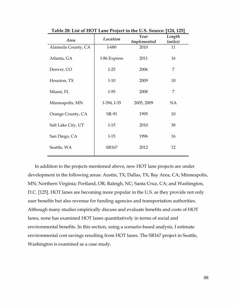
88

Table 28: List of HOT Lane Project in the U.S. Source: [124, 125]

Area Location Year

Implemented Length (miles)

Alameda County, CA I-680 2010 11

Atlanta, GA I-86 Express 2011 16

Denver, CO I-25 2006 7

Houston, TX I-10 2009 10

Miami, FL I-95 2008 7

Minneapolis, MN I-394, I-35 2005, 2009 NA

Orange County, CA SR-91 1995 10

Salt Lake City, UT I-15 2010 38

San Diego, CA I-15 1996 16

Seattle, WA SR167 2012 12

In addition to the projects mentioned above, new HOT lane projects are under

development in the following areas: Austin, TX; Dallas, TX; Bay Area, CA; Minneapolis,

MN; Northern Virginia; Portland, OR; Raleigh, NC; Santa Cruz, CA; and Washington,

D.C. [125]. HOT lanes are becoming more popular in the U.S. as they provide not only

user benefits but also revenue for funding agencies and transportation authorities.

Although many studies empirically discuss and evaluate benefits and costs of HOT

lanes, none has examined HOT lanes quantitatively in terms of social and

environmental benefits. In this section, using a scenario-based analysis, I estimate

environmental cost savings resulting from HOT lanes. The SR167 project in Seattle,

Washington is examined as a case study.

4.4.1 P

In 2008,

HOV la

lanes is

Fig

SR16

provide

motorcy

lane for

point alo

Acco

HOT lan

trip. Als

Project Backg

the Washi

nes along S

about 10 m

gure 18: SR

67 runs par

s six access

ycles, carpo

a fee. Figu

ong SR167.

ording to th

ne along SR

so WSDOT

ground

ington Stat

SR167 to H

miles from R

R167 HOT L

rallel to I-5

s points, an

olers, vanp

ure 18 show

he WSDOT

R167 is 3,400

reports ave

te Departm

HOT lanes

Renton, Was

Lane Projec

and provi

nd Southbou

poolers and

ws the proje

report [126

0 trips per w

erage peak

ment of Tran

[126]. The

shington to

ct Area, Sta

des access

und SR167

those solo

ct location

6], the avera

weekday, a

hour volum

nsportation

portion of

o Auburn, W

ate of Wash

to I-5 and

provides fo

drivers wh

as well as

age number

and the ave

mes of the g

n (WSDOT

SR167 con

Washington

hington Sou

I-405. Nor

our access p

ho wish to u

the location

r of tolled t

erage toll pa

general pur

) converted

nverted to H

n.

urce: [126]

rthbound S

points to bu

use SR167 H

n of each ac

trips using t

aid is $1.25

rpose lanes

89

d the

HOT

R167

uses,

HOV

ccess

the

per

90

have decreased 5 percent, and speed has increased over 20 percent. Speed along HOT

lanes is reported to remain at 60 mph.

4.4.2 Method and Results

To estimate the direct and indirect cost savings resulting from the SR167 HOT lane in

the State of Washington, performance measures reported by WSDOT [126] were used.

The report provides the following information:

‐ Speed on general lanes has increased 20 to 30 percent. Average speed at the time

of deployment in 2008 was 42 mph. For this analysis speed improvements of

51mph (lower bound) and 56 mph (upper bound) were used.

‐ Speed on HOT lanes remains at around 60mph.

‐ On average 2,950 solo drivers use HOT lanes on weekdays.

‐ Average daily traffic volume along SR167 is about 120,000.

Based on the above information and using the same method described in Sections

2.3 and 3.2.3, the fuel cost and the external environmental costs were estimated for the

base case (prior to the implementation of HOT lanes) and two after implementation

scenarios (lower bound and upper bound). The results are shown in Figure 19.

Figure 1

Altho

time for

the socie

in the St

translate

by the n

savings

pay mor

mph, the

are impl

Evalu

organiza

2012) we

19: Fuel and

ough imple

users, Figu

ety. Externa

tate of Wash

es into a tot

number of v

to the aver

re than they

ese drivers

lemented.

uating HOT

ations, the e

ere $820,00

d Environm

ementing H

ure 19 show

al environm

hington. A

tal daily sav

vehicles, eac

age toll rate

y save in fu

save about

T lanes from

expenditur

0 while the

mental Costthe State

HOT lanes h

ws HOT lan

mental costs

net savings

ving of app

ch vehicle s

e of $1.25 p

uel. Assumi

t 4 minutes

m the persp

es for the la

e revenue w

t Savings Re of Washin

helps agenc

nes result in

s are shown

s in total co

proximately

saves about

per trip, solo

ng that spe

along the s

pective of g

ast four qua

was about $9

Resulting frngton

cies raise re

n no change

n to increas

ost of fuel b

y $2,000. No

t 2 cents per

o drivers us

eed increase

stretch of th

government

arters repor

960,000, res

rom SR167

evenue and

e in air emis

se between

between 1 to

ormalizing

r day. Com

sing the SR

ed from 42

he road wh

t and plann

rted (April

sulting in $

7 HOT Lane

reduces tra

ssion costs

2 to 4 perce

o 2 percent

these savin

mparing the

R167 HOT la

mph to 56

here HOT la

ning

2011 – Mar

140,000 pro

91

es in

avel

to

ent

ngs

fuel

ane

anes

rch

ofit

92

for the WSDOT. Assuming the only social cost would be the external environmental

cost ($10,000/Day), the annual benefit cost ratio would be 0.6.

In Section 4.5 I discuss why one congestion management strategy (i.e. ATCS) results

in environmental cost savings while another strategy (i.e. HOT lanes) increases the

external environmental costs. Given that most transportation agencies are concerned

about climate change and many have developed GHG reduction plans, the choice of

congestion management measure and its alignment with the environmental objectives

becomes significant. Section 4.5 should provide guidance on the type of strategy that

agencies and decision makers choose to implement in order to reduce congestion and

promote urban environmental sustainability.

4.5 Congestion Management and Speed

Integrated assessment of congestion management and its consequential GHG emission

and air pollutants is quite limited. Barth [127] provides an analysis of carbon dioxide

emission reductions associated with speed mitigation, shock-wave suppression and

generalized congestion reduction. In particular, Barth’s study in Southern California

shows that GHG emissions resulted from traffic congestion can be reduced by about 20

percent through congestion management measures that improve speed in a way that

reduces CO2 emissions [127]. In addition to CO2, vehicles are sources of criteria air

pollutants such as NOx, CO and VOC. These criteria air pollutants not only are

responsible for negative health impacts, but, through interaction with Ozone (O3) and

methane (CH4), also have indirect effects on climate change [128]. Driving patterns and

speed have significant impacts on the emission of the criteria air pollutants. Therefore,

the relationship between congestion and air emissions cannot be evaluated ignoring

factors such as speed and driving patterns. In this section, I chart the relationship

between all air pollutants and speed intervals based on the emission factors provided

by EPA’s MOBILE6 software for light duty vehicles [31].

Figure 2

These pa

previous

At ab

environm

speeds.

which al

increase

that are

around 3

result, re

be consi

hope of

measure

20 shows th

articular sp

s section.

bout 52 mp

mental cost

Not shown

lso starts in

e with much

implement

30-35 mph,

elationship

idered befo

promoting

es reduce tr

he emission

peeds are th

Figure 20:

ph, CO2, CO

ts of those c

n in Figure

ncreasing at

h higher sp

ted along ar

, which is n

s between s

re impleme

g urban env

ravel time a

factors at s

hose that we

Emissions

O and VOC

congestion

20 is the re

t around 51

eeds. In con

rterials with

near the low

speed, traff

enting traffi

ironmental

and increase

speeds of 42

ere used for

s for Variou

start increa

manageme

elationship b

1 mph. NOx

ntrast, for c

hin urban a

w point of al

fic congesti

ic congestio

l sustainabi

e travel spe

2mph, 51m

r the analys

us Speed P

asing, resul

ent measure

between sp

x emissions

congestion m

areas (i.e. A

ll pollutant

on and urb

on managem

ility. While

eed, the latt

mph, 56 mph

sis of HOT

Profiles

lting in an i

es that resu

peed and fu

s, on the oth

manageme

ATCS), spee

t curves in F

ban air pollu

ment meas

congestion

ter improve

h and 60 mp

lanes in th

increase in t

ult in higher

uel energy,

her hand,

ent measure

ed is genera

Figure 19. A

ution need

sures with t

n managem

ement may 93

ph.

e

the

r

es

ally

As a

to

the

ment

not

94

be environmentally beneficial. Increasing speed may also have safety implications. To

obtain a net social benefit from implementing a congestion management strategy, all

first order and secondary impacts should be taken into consideration.

95

“When a road is once built, it is a strange thing how it collects traffic.”

Robert Louis Stevenson (1850-1894)

96

Chapter 5

Rebound Effects for Induced Demand Due to Supply Changes

5.1 Types of Rebound Effects

In chapters 3 and 4, a select number of demand and supply congestion management

measures were assessed for cost-effectiveness and potential to reduce the impact of the

transportation system on the environment and to promote urban environmental

sustainability. While I analyzed each of these strategies in isolation, in Chapter 3 land

use strategies were combined with building standards (i.e. LEED) and smart growth

principles to assess the synergic and marginal impact they have on the external

environment costs. In this chapter, I examine the interconnectivity of supply congestion

management measures from a rebound effect perspective, and how rebound effects can

impact the net benefits resulting from implementing a congestion management

measure. Rebound effects within the realm of light duty vehicles can be categorized into

three groups:

1- Induced Demand (direct volume change): Implementing congestion management

measures and improving operations in an urban network could free up some of

the congested capacity and result in newly generated traffic. With the newly

generated traffic, the network can be pushed towards a new equilibrium point,

hence reducing the net economic and environmental benefits.

2- Income Elasticity: Abandoning private vehicles due to better accessibility to job

sites or transit might result in higher spending power (i.e. spending fuel savings

on energy consuming goods, spending time savings on energy inefficient

activities), which in turn can reduce the net economic and environmental benefits

originally expected from implementing the strategy.

3- Transit Demand: Shifting people from suburbun to urban areas through land use

changes may reduce traffic regionally but adds to the local traffic. This

phenomenon can result in higher demand for other modes of transportation such

97

as transit, which, in turn, can potentially reduce the net environmental benefits.

Beyond a certain demand, transit agencies need to add vehicles to the existing

fleet. Adding transit vehicles to the existing fleet may impact the cost

effectiveness of the entire system economically and environmentally.

While each of the categories is important in the holistic analysis of urban

environmental sustainability and cost-effectiveness of congestion management

measures, in this chapter I mainly focus on the first category, induced demand caused

by direct change in volume and due to excess capacity. Using scenario-based analysis

from the previous chapters, I estimate the effectiveness of congestion management

measures and at what point the travel network reaches equilibrium as a result of the

newly generated traffic.

5.2 Induced Demand by Direction Change in Volume

Economic theory of supply and demand from neo-classical microeconomic theory

[129-131] can simply and thoroughly explain the phenomena called induced demand.

By implementing supply congestion management strategies and increasing the carrying

capacity of roadways, the cost of travel decreases. This cost includes cost of time, as well

as operating costs (i.e. fuel and maintenance). As cost decreases, demand increases, both

due to the reduction of cost itself and an increase in available income by users.

Figure 21 illustrates the demand and supply equilibrium effects due to a price

decline for a service.

Figur

The o

congesti

cost for

supply i

a result

induced

capacity

1) L

b

13

2) P

b

L

P3

re 21: Dema

original equ

ion manage

driving (P2

is shortened

the cost of

d demand o

y can be gen

Light duty v

ut using ot

33].

People who

ut due to th

LDV.

and and Su

uilibrium is

ement strate

2), demand

d, therefore

service dem

r newly gen

nerated by t

vehicle (LD

her routes

have been

he reduced

upply ChanManage

s at the inte

egy and inc

increases (Q

e price incre

manded (in

nerated tra

two groups

V) drivers t

or times to

using other

cost of trav

nges Due toement Mea

ersection of

creasing the

Q2). As dem

eases (P3), r

this case fr

ffic. The inc

s:

that are alre

travel from

r modes of

vel, decide

o Implemenasure

f Q1 and P1.

e supply, w

mand increa

resulting a n

ree flow dri

creased dem

eady travel

m their orig

travel (i.e.

to change t

ntation of a

By implem

which transl

ases (Q3), o

new equilib

iving) incre

mand for th

ling within

in to destin

transit, wa

their mode

a Congestio

menting a

lates to less

nce gain

brium poin

eases due to

he increased

n the networ

nation [132,

alking, bikin

of travel to

98

on

s

nt. As

o

d

rk

ng),

o

99

While both groups may contribute to the reduction in environmental benefits of

congestion management measures, the second group can potentially have more of a

significant impact as this group adds extra VMT to the network. In addition, reducing

the cost of travel can encourage commuters to live farther from the urban core and can

encourage sprawl [134], and thus work against urban environmental sustainability. In

this chapter, induced demand resulting from implementing congestion management

measures are estimated using a scenario-based analysis. The goal is not to say that

congestion management measures result in zero environmental benefit but to estimate

the impact they might have on the net impact.

5.2.1 Existing Induced Demand Assessments

Many studies have made an attempt to quantify the demand induced by increasing the

capacity of a transportation network. In fact the early studies on this topic date back to

1938, when a report was done for the UK Ministry of Transport on induced demand

due to construction of a new road [135]. Most studies have assumed some level of

elasticity between travel demand and capacity, meaning that, as capacity increases,

demand increases, and have estimated the elasticity [136-144]. Over the past two

decades, most of the travel demand elasticity studies have estimated the elasticity of

demand with respect to fuel price. Demand with respect to fuel price elasticity has

received significant attention over the last few years due to the volatility of gas prices

[145-150]. A number of studies have also estimated the elasticity of VMT with respect to

travel time [135, 151, 152]. Figure 22 compares the existing travel demand elasticity

assessments from various studies.

The s

based on

etc.). Th

0.4) com

In th

Townsh

simulati

informa

descript

5.2.2

To estim

various

simulati

simulati

Induced

average

The C

improve

Figu

studies illu

n data colle

e range of e

mpared with

his study, I

hip study as

ion data to

tion on the

tion of the s

Method a

mate elastici

percentage

ion model o

ion model f

d demand w

difference

Cranberry T

e the signal

ure 22: Exist

strated in F

ected in yea

elasticity es

h ranges of

use signal t

ssessed in S

measure el

project loc

signal timin

nd Results

ity of travel

e, starting w

of the Cranb

from Sectio

was forced i

between pe

Township s

operations

ting Travel

Figure 22 ha

ars prior to

stimated wi

elasticity w

timing and

Section 4.2 a

asticity of d

ation in Cr

ng project m

l demand w

with 2 perce

berry Town

n 4.2.3 was

into the AM

erformance

signal netw

s along the

l Demand E

ave estimat

each study

ith respect t

with respect

d traffic volu

and combin

demand wi

anberry To

may be foun

with respect

ent addition

nship netwo

s used to co

M, midday a

e measures

work was fir

network. T

Elasticity A

ted elasticit

y (i.e. gas pr

to gas is sm

t to lane mi

ume data fr

ne these dat

ith respect t

ownship, Pe

nd in Sectio

t to travel t

nal volume,

ork. The sa

onduct the r

and PM pea

for each pe

rst analyzed

The main str

Assessment

ty of deman

rice, travel t

maller (betw

iles and trav

rom the Cra

ta with fore

to travel tim

ennsylvania

on 4.2.

ime, induce

, was forced

ame Synchr

rebound an

ak periods

eak period.

d and optim

rategy used

ts

nd mostly

time, VMT,

ween - 0.1 to

vel time.

anberry

ecasted

me. Detailed

a, and a

ed demand

d into the

ro/SimTraff

nalysis.

to estimate

mized to

d to optimiz

100

,

o -

d

d of

fic

e the

ze

101

travel time and speed was to change the grouping of the intersections in order to have

shorter cycle lengths. Currently, the Cranberry Township has all its signals in two

groups of cycle lengths. To accommodate for all signals within each group, signals are

running with cycle lengths as long as 140 seconds. While 140 seconds might be

necessary for some of the intersections, this cycle length is too long for most of them.

Unnecessarily long cycle lengths cause side street traffic to wait for a long time,

resulting not only in residents and commuters’ frustration, but also in air emissions

while idling. As a result of changing cycle lengths and regrouping to better

accommodate most intersections in the Cranberry Township network, delays were

reduced by an average of 14 percent and travel time decreased by an average of 8

percent.

To estimate elasticity of demand with respect to travel time, travel volumes were

increased at various intervals, and the simulation model was run for an hour at each

induced demand interval. The results illustrated in Figure 23 shows that between 4 to 5

percent induced demand, the system reaches the same level of delay and travel time as

the existing condition. In other words, if demand increases by about 4.5 percent,

improvements made to the traffic signal system to increase capacity and reduce

congestion become obsolete and further improvement are necessary to maintain an

efficient traffic system and flow. In Figure 23 the y axis shows delay and travel time in

hour and each bar shows percent volume increase and its associated speed. For

instance, the first bar from the left side, shows the status quo situation, where the

average speed of the network is 20 mph. The second bar shows that with some

improvements made to the signal timing, delay decreases while the average speed of

the network remains at 20 mph. The third bar shows that three percent additional

demand is added to the network in one year, resulting in an increased delay while

speed remains the same.

Fig

From

-0.85, wh

increase

other stu

aligned

Assu

demand

gure 23: Tra

m these data

hich means

e in demand

udies menti

with the ela

Figur

uming a 10

d, the induc

avel Time a

a, the elasti

s that a 10 p

d. Figure 24

ioned in Se

asticity stud

re 24: Elasti

percent dec

ed demand

and Delay C

city of dem

percent decr

4 shows wh

ection 5.2.1

dy done by

icity of Dem

crease in tra

d will lower

Changes w

mand with r

rease in tra

here this stu

[135, 151, 1

y Sactra [151

mand with

avel time re

r the perfor

with respect

respect to tr

avel time re

udy falls in

152]. The res

1].

h respect to

esults in 8.5

rmance mea

t to Induced

ravel time i

sults in 8.5

comparison

sult of this

Travel Tim

5 percent in

asures sign

d Demand

s estimated

percent

n with the

study is

me

ncrease in

nificantly. Sp

102

d at

peed

103

decreases by 10 percent compared with the status quo situation, and delay increases by

about 20 percent.

Based on this analysis, the growth rate factor that results in the same hours of delay

as what the Cranberry roadway network is experiencing today was estimated to be 4.5

percent. The growth rate factor is estimated as:

GR = (1+r)y (5)

Where:

GR: Growth rate

r: annual rate of growth

y: number of years before the level of growth is reached

Assuming a national predicted annual VMT growth rate of 1.3 percent [10] along the

network, the system will require about 3.5 years to reach the same level of congestion as

today. This estimation is a reasonable indication that implemented signal timings must

be reevaluated no later than 3.5 years after when they were first deployed.

In short, when planning to implement a congestion management strategy, agencies

and decision makers need to understand the demand that will be generated due to the

improvements made to their system. Induced demand directly impacts cost

effectiveness of the strategy implemented and, in most cases, reduces the net benefit. It

is important to take into account in what time period the system reaches equilibrium

and what the plan might be at that point. In the case of signal timing and coordination,

it is relatively easy to manage induced demands, as reevaluating and adjusting the

timings to meet the new demand do not incur significant costs ($3,700 per intersection

based on Section 4.2.5.). Implementing more costly strategies such as Adaptive Signal

Control Systems, which require a significant amount of initial investment, needs careful

consideration as induced demand might lower the net benefit of the system

significantly.

104

5.3 Policy Implications of Induced Demand

Induced demand, as it was discussed in this chapter, reduces the benefits resulting from

the implementation of supply congestion management strategies. By adding extra

capacity to roadways – whether through adding lanes or improving traffic flow – traffic

delay decreases, travel time and speed increase and users are encouraged to drive more

frequently and for longer distances. Therefore, in a short to medium term timeframe the

roadway network reaches a new point of equilibrium, where demand and supply are

equal or demand is greater than supply, hence traffic congestion. In short, the benefits

resulting from the deployment of supply congestion management measures are

generally short lived. Therefore, to assess the net benefit of a supply congestion

management measure, elasticity of demand with respect to price (i.e., travel time, delay)

needs to be included in the analysis. Policy makers and especially funding agencies

need to evaluate each strategy in a short, medium and long term timeframe before

deciding on the feasible amount of funding to be invested on a strategy. While short

term benefits are most probable for supply congestion management measures, in a

medium to long term timeframe these measures may lead to zero net benefit. In

addition, induced demand results in external social costs such as accidents, noise

pollution and environmental damages. Policy makers need to include all social costs in

the cost effectiveness analyses performed to gauge the net benefit of a given strategy.

In the U.S., transportation decision makers mainly consider immediate performance

measures resulting from the implementation of a congestion management measure.

These performance measures are delay, speed and travel times. Upon implementation

of a supply congestion management measure, the agencies typically perform an

evaluation to examine immediate improvements resulting from the deployment of the

strategy. It is seldom that the agencies would repeat the evaluation process after six

months, a year or beyond to evaluate the medium to long term impacts of the

implemented strategy, including the effects of induced demand. This process is

encouraged by two factors:

105

‐ Local transportation agencies and policy makers rely heavily on the state and

national funding sources. These funding sources are typically specific to projects

(i.e., funding for signal timing projects), taking the liberty of the local authorities

to decide the best use for the funding away. In cases where funding is not

allocated to a specific type of a project, the timeline to decide on allocations is

typically short, leaving authorities with limited implementation options.

‐ Local transportation authorities are encouraged to show immediate

improvements to sustain their funding or to be able to apply for subsequent

rounds of funding. As a result, most agencies deploy those supply management

strategies that would result in the greatest short term benefits, without much

consideration for long term user and social benefits.

Induced demand studies, such as the one examined in this chapter, should

encourage policy makers and funding sources to consider the impacts of induced

demand in their cost effectiveness analyses, while deciding which projects to fund. It is

only through a holistic cost effectiveness analysis of congestion management strategies

that long term urban transportation sustainability may be achieved. When it comes to

induced demand and congestion management, the key policy point is that while all

strategies result in some level of benefits in a short term timeframe, not every strategy

results in medium to long term benefits. Therefore, decision makers should encourage

local transportation authorities to evaluate their implemented congestion management

strategies not only frequently, but also regularly throughout the lifetime of the strategy.

As part of this process the current funding structure needs to change to accommodate

for long term evaluation of the projects. In addition, to effectively evaluate the results of

an implemented project in long term, performance measures other than the traditional

ones (i.e., delay and speed) need to be considered. Social performance metrics such as

environmental damages, health impacts and safety should be introduced into the long

term evaluation processes.

106

"The only way to solve the traffic problems of the country is to pass a law that only paid-for cars are allowed to use the highways. That would make traffic so scarce we could use the boulevards for children's playgrounds."

-Will Rogers (1879 – 1935)

107

Chapter 6

Conclusions

In the previous five chapters, we discussed the impact of vehicle miles traveled and

traffic congestion on the environment and GHG emissions resulting from the

transportation sector. The external environmental cost of traffic congestion in the U.S.

was estimated, and the economic and environmental costs and cost savings associated

with a number of supply and demand travel and congestion management measures

were assessed. Strategies examined on the demand side were land use, including

brownfield and infill developments and smart growth transportation principles within

the LEED standard including parking pricing, bike lanes and storages and pedestrian

walkways. Strategies examined on the supply side were proactive maintenance and

evaluation of signal timing and coordination, adaptive signal timing and high

occupancy toll lanes. Two main differentiating factors between this work and other

existing literature are:

1. This works examines demand and supply side strategies in terms of their health

(mortality and morbidity) and environmental impacts in monetary values.

2. This work assesses the interdependencies that might exist in between the

strategies and their outcomes in terms of newly generated traffic, and speed

profiles, as well as marginal benefits of implementing some of the strategies as a

group.

The result of this work shows the external environmental cost of traffic congestion in

the metropolitan areas of the U.S. is approximately $16 billion a year or about $260 per

household per year (assuming 61 million households in the U.S. metropolitan areas

based on the population of 158 million and household density of 2.6 [109]). This

estimate includes costs of mortality, morbidity and environmental damages resulting

solely from traffic congestion. Total environmental cost of driving including congestion

was estimated to be $110 billion per year for all the U.S. urban areas or $1,080 per

househo

use strat

reductio

per year

environm

induced

that imp

strategie

congesti

address

newly g

demand

Fig

old per year

tegies such

on strategie

r. Supply m

mental ben

d demand (i

plementing

es) results in

ion to local

the newly

generated co

d. Figure 25

gure 25: Rel

r. To reduce

as brownfi

s, such as p

management

nefit due to

i.e. in case o

land use st

n shifting t

roads and

added traff

ongestion o

illustrates

lationship bE

e the enviro

ield or infil

parking pric

t strategies

two issues:

of signal tim

trategies alo

he regional

calling for

fic. Supply

on local roa

the cycle:

between TrEnvironmen

onmental co

l developm

cing, can sa

show less o

: speed prof

ming and co

one (withou

l VMT to lo

supply con

manageme

ds by addin

ransportatintal Sustai

osts of driv

ments combi

ave an aver

of a certain

files (i.e in

oordination

ut other de

ocal VMT, t

ngestion ma

ent strategie

ng capacity

ion Measurinability

ving and co

ined with d

rage of $450

n and long t

case of HO

n). It was al

mand man

therefore ad

anagement

es, while ad

y, can gener

res to Achi

ongestion, la

demand

0 per house

term net

OT lanes) an

lso discusse

nagement

dding traffi

measures t

ddressing th

rate new

ieve Urban

108

and

ehold

nd

ed

c

to

he

109

Direct emission control is a component of the diagram in Figure 25 that has not been

considered or analyzed in this work. Within the context of urban environmental

sustainability, reducing emissions through fuel and vehicle direct emissions control

strategies is an important factor. In this chapter, I discuss the direct emission control

component of Figure 25. This is not to introduce new information, rather the objective is

to discuss the already assessed travel demand and congestion management measures as

a strategy to attain GHG emission reduction goals relative to other transportation

strategies such as direct emissions control.

6.1 Fuel and Vehicle Direct Emissions Control Strategies

As mentioned earlier in this work, to reduce GHG emissions federal and state mandates

are in place for low carbon fuels and fuel efficient vehicles. The new CAFE standard

requires a large increase in the average fuel economy of LDVs; increasing fuel economy

from the current average of 22.4 mpg to 56 mpg by 2025 [12, 13]. Based on the direct

relationship between gasoline fuel use and CO2 emissions, the implementation of fuel

efficient vehicle technologies and low carbon fuels, combined with motivating

consumers to choose these vehicles will be critical for reducing GHG emissions from the

LDV fleet. Change however has been slow in the U.S., mainly due to the low cost of

conventional vehicles relative to alternative fuel vehicles. Consumers generally favor

conventional light duty vehicles because of their low cost of operation and low gasoline

tax. The higher cost and limited availability of new technologies, unwillingness of

consumers to adopt the new technologies, and the significant infrastructure changes

required to develop and market advanced fuels and vehicles contribute to the limited

adoption of alternatives.

In terms of alternative fuel and vehicle technologies, while a number of options can

potentially result in significant reductions in GHG emissions, none are expected to

achieve the “50 to 80 percent below 2000 levels” reduction goal by 2050 recommended

by the Intergovernmental Panel on Climate Change (IPCC) [153]. Extensive adoption of

110

more fuel efficient vehicles such as diesels, hybrid electric vehicles (HEV) or advanced

conventional vehicles can reduce emissions by 15 to 30 percent per mile of travel [36, 37,

154]. Biofuels such as E85 (85 percent ethanol and 15 percent gasoline) could have

varying results depending on the type of feedstock and its fuel production pathway

[155]. Furthermore, uncertainties associated with land use change occur when land is

converted to produce feedstock [156]. Fuel cell vehicles using hydrogen can result in

GHG emission reductions only if low carbon sources of hydrogen can be obtained in

large quantities [157]. Many studies show that electric vehicles result in life cycle GHG

emissions reductions [36, 157, 158]. Electric vehicles impact on GHG emissions is

uncertain because of the existing electric power generation issues. Consistent with the

valuation method used in this work, Michalek et al. [36] estimate the external costs

associated with the life cycle air emissions of plug-in-hybrid-electrical vehicles (PHEV)

with small battery sizes charged using low-carbon or renewable sources to be $800

lower than conventional vehicles. Savings are in the reduction of CO, PM2.5, VOC and

GHG. While these studies estimate emission reductions, they all assume renewbale

power for charging purposes. In reality, however, using renewable power to always

charge vehicles is improbable, at least within the next few decades. Power plants across

the U.S. balance demand and supply by using different types of fuel. Wind and solar

resources are intermittent. The net impact of electric vehicles on GHG emissions,

therefore, largely depends on the system-wide impacts of charging the vehicles and all

that is involved from the power plant side (i.e. time of charging, electricity generation

mix, grid operations). Other potential fuel and vehicle technologes such as algae

biodiesel are early in the development stage with significant uncertainties on their

impact on GHG emission reduction.

In summary, direct emission control strategies such as fuel and vehicle changes can

reduce GHG emissions. However, the reductions most likely will not achieve the 50 to

80 percent goal estimated by IPCC, but far less.

111

6.2 Discussion

The combined results of this work suggest that a single transportation strategy would

not be sufficient to achieve substantial transportation GHG reductions. To effectively

achieve GHG emission reduction goals and to promote urban environmental

sustainability, combinations of strategies including direct emission control strategies

(Section 6.1), land use strategies (Section 3.2), demand management strategies (Section

3.3) and supply management strategies (Section 4.1) are needed (Figure 25).

Transportation strategies can be mutually reinforcing. In fact, none of the strategy

categories alone is likely to have greater than a moderate impact on GHG emissions.

Among the four categories of strategies discussed (fuel/vehicle technologies,

demand management, land use and supply management), demand management

strategies, while having small to moderate impact on GHG emissions by themselves,

result in the highest impact if combined with the other three strategies. Travel demand

management strategies combined with land use changes reduce local traffic congestion

and its consequential GHG emission by providing more compact and walkable

communities (i.e. LEED combined with brownfield development (Chapter 3)). Travel

demand management strategies combined with supply management strategies reduces

induced demand caused by extra capacity (Chapter 5). Lastly travel demand

management strategies combined with fuel and vehicle strategies reduce the amount of

travel and thereby avoid range constraints with battery electric vehicles or gasoline

driving plug-in hybrid electric vehicles.

In the case of land use strategies and their combination with demand management

strategies (the main focus of this work), the objective is to ultimately lower the number

of trips and shorten the length of trips. Various forms of this combination are:

‐ Compact developments with higher density and less parking, resulting in less

travel activity

‐ Mixed use developments with multiple services and types of land use within one

area, resulting in fewer number of trips and shorter length of trips

112

‐ Pedestrian and bicycle friendly developments with bike and pedestrian

networks, connectivity, safety and an aesthetic environment, promoting less

travel activity

‐ Transit oriented developments with close proximity and accessibility to transit

services, reducing the number of trips

‐ Infill/brownfield developments within the urban core for close proximity to

various land uses and transit to reduce number of trips and the length of trips

While each of these developments has the potential to reduce carbon intensive travel

activity, combining them would result in synergistic impact on VMT reduction.

Therefore, in achieving the maximum reduction in travel activity and its associated

GHG emissions, the key is to combine as many possible elements of each of the

developments (i.e., compact, parking pricing, access to transit, mixed use, bikeways,

pedestrian pathways, etc.).

In addition, to successfully moving towards urban environmental sustainability,

cooperation and collaboration between public agencies on local, state and regional

levels as well as between public and private entities is crucial. The goal should be to

create platforms, tools and processes that enhance this collaboration and to make

decisions collaboratively and effectively. As an example, land use strategies with a high

potential of travel reduction when combined with demand management strategies

incur minimal cost to the regional and federal transportation authorities and

metropolitan planning organizations, as most of the cost is paid by private entities and

developers. Public agencies can provide incentives and guidelines to ensure the design

implementation of smart growth elements and demand management strategies that

would result in higher personal travel reduction. Incentives can be provided so that

developers are encouraged to develop those sites that are near transit and other service

areas. Moreover, guidelines can be enforced for the design of walkable streets,

connectivity factors, safety and aesthetic elements. Through such collaboration between

public agencies and private developers not only is travel activity and its associated

113

GHG emissions reduced, but also co-benefits such as increased physical activity, fewer

accidents, and increased transit ridership are expected. Another important co-benefit

can be increasing the economic growth of central cities in the U.S. As mentioned in

Chapter 3, brownfield developments showed a 9 percent vacancy rate compared to 1

percent vacancy rate of conventional developments. Through collaboration between

public agencies and private entities, the vacancy rate in brownfield developments can

be reduced not only by implementing demand management strategies that potential

residents find attractive but also by providing incentives to those residents moving into

the developments. Implementing demand management strategies such as connectivity

and safe walkways encourages those entering their aging years to move into the

developments, while providing incentives to potential residents encourages younger

generations to occupy the infill developments. Lowering the rate of vacancy would

result in advancing economic growth, especially in the underutilized urban core areas.

6.3 Research Contributions

Assessing and estimating the impacts of the transportation sector on GHG emissions

and strategies to alleviate those impacts have been discussed and published before [8,

40, 41]. That said, the relationship between these strategies, their marginal impacts if

implemented in combination, and how they interact with each other are all important

factors in determining their net impact on GHG emissions. Key points from this

research are:

‐ External environmental costs of traffic congestion and cost savings resulting

from congestion management measures are significant.

‐ No one strategy, whether land use or congestion management, will be sufficient

to achieve urban environmental sustainability; rather it is the net impact of

strategies and the synergies between them that can potentially produce

significant impacts.

‐ Travel demand management measures combined with supply management

measures, land use strategies and fuel/vehicle emission control strategies can

114

have a significant marginal impact on alleviating GHG emissions and increasing

economic growth due to lower vacancy rates in land use developments.

‐ Although congestion management measures reduce delay and travel time, not all

supply measures reduce GHG emissions. Speed improvements determine

whether strategies are environmentally beneficial.

‐ Demand induced as a result of implementing a travel reduction and/or

congestion management measure can have a significant impact on the net benefit

of the measure itself.

‐ Collaboration among public agencies and private entities to provide incentives

and guidelines is necessary to achieve the maximum possible net benefit of

demand and supply travel management measures.

115

Bibliography

[1] USCensus. 1103 - Motor Vehicle Accidents--Number and Deaths [Online]. Available: http://www.census.gov/compendia/statab/2012/tables/12s1103.pdf

[2] Y. Mashayekh, P. Jaramillo, M. Chester, C. T. Hendrickson, and C. L. Weber, "Costs of automobile air emissions in US metropolitan areas," Transportation Research Record: Journal of the Transportation Research Board, vol. 2233, pp. 120-127, 2011.

[3] I. W. H. Parry, M. Walls, and W. Harrington, "Automobile externalities and policies," Journal of Economic Literature, pp. 373-399, 2007.

[4] D. Schrank and T. Lomax, "The 2011 urban mobility report," Texas Transportation Institute, pp. 1-57, 2011.

[5] U. EPA, "Inventory of U.S. Greenhouse Gas Emissions and Sinks: 1990-2010," Environmental Protection Agency2012.

[6] S. Davis, S. Diegel, and R. Boundy, "Transportation Energy Data Book," Oak Ridge National Laboratory, vol. Edition 31, 2012.

[7] F. Sissine, "Energy Independence and Security Act of 2007: a summary of major provisions," 2007.

[8] USDOT, "Transportation’s role in reducing US. Greenhouse Gas Emissions " U.S. Department of Transportation, Washington D.C.2010.

[9] FHWA. (2010). Highway Statistics 2010. Available: http://www.fhwa.dot.gov/policyinformation/statistics/2010/vm1.cfm

[10] EIA, "Annual Energy Outlook 2012," Energy Information Administration, U.S. Department of Energy DOE/EIA-0383(2012), 2012.

[11] AASHTO, "Primer on Transportation and Climate Change," The American Association of State Highway and Transportation Officials. , 2008.

[12] F. Register, "Light-Duty Vehicle Greenhouse Gas Emission Standards and Corporate Average Fuel Economy Standards," Final Rule. 25324, vol. 75, 2010.

[13] F. Register, "2017 and Later Model Year Light-Duty Vehicle Greenhouse Gas Emissions and Corporate Average Fuel Economy Standards," 74854, vol. 76, 2011.

[14] A. e. A. Altshuler, "The Urban Transportation System: Politics and Policy Innovation," ed: Cambridge, Mass.: MIT Press. THE EVOLUTION OF THE URBAN INFRASTRUCTURE IN THE NINETEENTH AND, 1979.

[15] T. Litman, "Transportation cost and benefit analysis, techniques, estimates and implications, viewed 1 March 2010," ed, 2009.

[16] M. A. Delucchi, The annualized social cost of motor-vehicle use in the US, 1990-1991: Summary of theory, data, methods, and results: Citeseer, 1999.

[17] H. S. Matthews and L. B. Lave, "Applications of environmental valuation for determining externality costs," Environmental Science & Technology, vol. 34, pp. 1390-1395, 2000.

[18] P. Miller and J. Moffet, "The Price of Mobility: Uncovering the Hidden Costs of Transportation," 1993.

[19] M. Maibach, C. Schreyer, D. Sutter, H. Van Essen, B. Boon, R. Smokers, et al., "Handbook on estimation of external costs in the transport sector," Report, Delft, pp. 23-35, 2008.

116

[20] K. Saito, T. Kato, and T. Shimane, "Traffic Congestion and Accident Externality: A Japan-US Comparison," The BE Journal of Economic Analysis & Policy, vol. 10, 2010.

[21] J. Granell, C. Ho, T. Tang, and M. Claggett, "Analysis of MOBILE6. 2’s PM Emission Factor Estimating Function," in Proc., US Environmental Protection Agency’s 13th International Emission Inventory Conference, 2004, pp. 8-10.

[22] D. D. Parrish, "Critical evaluation of US on-road vehicle emission inventories," Atmospheric Environment, vol. 40, pp. 2288-2300, 2006.

[23] M. V. Chester, A. Horvath, and S. Madanat, "Comparison of life-cycle energy and emissions footprints of passenger transportation in metropolitan regions," Atmospheric Environment, vol. 44, pp. 1071-1079, 2010.

[24] N. R. C. C. o. Health, O. E. Costs, B. o. E. Production, N. R. C. B. o. E. Studies, N. R. C. B. o. Energy, E. Systems, et al., Hidden Costs of Energy: Unpriced Consequences of Energy Production and Use: National Academy Press, 2010.

[25] N. Z. Muller, R.O. Mendelsohn., "Measuring the Damages from Air Pollution in the U.S.," Journal of Environmental Economics and Management, pp. 1-14, 2007.

[26] K. Small and C. Kazimi, "On the costs of air pollution from motor vehicles," Journal of Transport Economics and Policy, vol. 29, pp. 7-32, 1995.

[27] I. Mayeres, S. Ochelen, and S. Proost, "The marginal external costs of urban transport," Transportation Research Part D: Transport and Environment, vol. 1, pp. 111-130, 1996.

[28] O. Johansson, D. Pearce, and D. Maddison, True costs of road transport. UK: Earthscan, 1996.

[29] D. McCubbin and M. Delucchi, "The health costs of motor-vehicle-related air pollution," Journal of Transport Economics and Policy, vol. 33, pp. 253-286, 1999.

[30] A. K. Sen, G. Tiwari, and V. Upadhyay, "Estimating marginal external costs of transport in Delhi," Transport Policy, vol. 17, pp. 27-37, 2010.

[31] EPA, "MOBILE6 Vehicle Emission. Modeling Software.," 2003. [32] D. Schrank and T. Lomax, "The 2007 urban mobility report," Texas Transportation

Institute, pp. 1-60, 2009. [33] M. Ross, "Automobile fuel consumption and emissions: Effects of vehicle and driving

characteristics," Annual Review of Energy and the Environment, vol. 19, pp. 75-112, 1994.

[34] N. Z. Muller, "Linking policy to statistical uncertainty in air pollution damages," The BE Journal of Economic Analysis & Policy, vol. 11, 2011.

[35] H. S. Matthews, C. Hendrickson, and A. Horvath, "External costs of air emissions from transportation," Journal of infrastructure systems, vol. 7, pp. 13-17, 2001.

[36] J. J. Michalek, M. Chester, P. Jaramillo, C. Samaras, C. S. N. Shiau, and L. B. Lave, "Valuation of plug-in vehicle life-cycle air emissions and oil displacement benefits," Proceedings of the National Academy of Sciences, vol. 108, pp. 16554-16558, 2011.

[37] A. Burnham, M. Wang, and Y. Wu, "GREET 2.8 Transportation Vehicle-Cycle Model," Argonne National Laboratory, Argonne, IL2008.

[38] U. S. B. o. L. Statistics., "Consumer Price Index. ," U.S. Department of Labor, 2010. [39] R. Johnston, "Review of US and European regional modeling studies of policies intended

to reduce motorized travel, fuel use, and emissions," Victoria, British Columbia: Victoria Transport Policy Institute, 2006.

117

[40] R. Ewing, K. Bartholomew, S. Winkelman, J. Walters, and D. Chen, Growing Cooler: The Evidence on Urban Development and Climate Change (Washington, DC: Urban Land Institute), 2008.

[41] NRC, "Special Report 298- Driving and the built environment: the effects of compact development on motorized travel, energy use, and CO2 emissions," Transportation Research, The National Research Council of the National Academies, 2009.

[42] S. Handy, X. Cao, and P. Mokhtarian, "Correlation or causality between the built environment and travel behavior? Evidence from Northern California," Transportation Research Part D: Transport and Environment, vol. 10, pp. 427-444, 2005.

[43] M. Shammin, Herendeen, R., Hanson, M. and Wilson, E., "A multivariate analysis of the energy intensity of sprawl versus compact living in the US for 2003," Ecological Economics, vol. 69, pp. 2363-2373, 2010.

[44] P. Gordon and H. Richardson, "Are Compact Cities a Desirable Planning Goal?," Journal of the American Planning Association, vol. 63, pp. 95-106, 1997.

[45] R. O'Toole, "The Myth of the Compact City Why Compact Development Is Not the Way to Reduce Carbon Dioxide Emissions," Policy Analysis, 2009.

[46] E. Paull, "The Environmental AND Economic Impacts OF Brownfields Redevelopment," Northeast Midwest, 2008.

[47] G. W. University, "Public Policies and Private Decisions Affecting the Redevelopment of Brownfields: An Analysis of Critical Factors, Relative Weights and Areal Differentials," 2001.

[48] C. De Sousa, "Policy Performance and Brownfield Redevelopment in Milwaukee, Wisconsin," The Professional Geographer, vol. 57, pp. 312-327, 2005.

[49] T. U. C. o. Mayors, "Clean Air/Brownfields Report," Environmental Protection, 2001. [50] EPA, "Solving Environmental Problems through Collaboration: the Atlantic Steel," U.S.

Environmental Protection Agency, Washington D.C. EPA-231-F-06-002, June 2006 2006.

[51] EPA, "Air and Water Quality Impacts of Brownfields Redevelopment " U.S. Environmental Protection Agency, Washington D.C. EPA 560-F-10-232, April 2011 2011.

[52] A. Nagengast, C. Hendrickson, and D. Lange, "Commuting from US Brownfields and Greenfield Residential Development Neighborhoods," ASCE Journal of Urban Planning and Development, vol. 137, pp. 298-304, 2011.

[53] EPA, "Brownfields and Land Revitalization," Environmental Protection Agency, 2009. [54] U. GAO, "BROWNFIELD REDEVELOPMENT H ighlights," in Program, 2004. [55] U. D. o. H. a. U. Development, "HUD Aggregated USPS Administrative Data On

Address Vacancies.," 2010. [56] U. Congress, "Office of Technology Assessment (1995): The Technological Reshaping

of Metropolitan America," OTA-ETI-643. Washington, DC: US Government Printing Office1995.

[57] D. Lange and S. McNeil, "Clean It and They Will Come? Defining Successful Brownfield Development," Journal of Urban Planning and Development, vol. 130, p. 101, 2004.

[58] D. Kaufman, And Cloutier, N., "The Impact of Small Brownfields and Greenspaces on Residential Property Values.," Journal of Real Estate Finance and Economics, pp. 19-30, 2006.

118

[59] U. S. E. P. Agency, "EPA Remediation Technology Cost Compendium – Year 2000," 2001.

[60] R. R. Rast, "Environmental remediation estimating methods," 1997. [61] CUED, "Brownfields Redevelopment: Performance Evaluation," Washington D.C., 1999. [62] C. B. Initiative, " Recycling Our Past, Investing in Our Future. ," 2003. [63] R. Burchell, A. Downs, B. McCann, and S. Mukherji, Sprawl costs: Economic impacts of

unchecked development: Island Press, 2005. [64] C. B. Leinberger, The option of urbanism: Investing in a new American dream: Island

Press, 2009. [65] A. A. Altshuler, J. A. Gomez-Ibanez, and A. M. Howitt, Regulation for revenue: The

political economy of land use exactions: Brookings Institution Press, 1993. [66] R. Burchell, N. Shad, D. Listokin, H. Phillips, A. Downs, S. Seskin, et al., "TCRP Report

39: The Costs of Sprawl- Revisited. TRB, National Research Council, Washington, D. C., ," 1998.

[67] M. Greenberg, "Should housing be built on former brownfield sites?," Journal Information, vol. 92, 2002.

[68] X. Wang and R. Vom Hofe, Research methods in urban and regional planning: Springer, 2007.

[69] H. J. Miller and S. L. Shaw, Geographic information systems for transportation: principles and applications: Oxford University Press, USA, 2001.

[70] C. B. Initiative, "Recycling Our Past, Investing in Our Future," 2003. [71] R. Auld, Hendrickson, C., and Lange, D., "A Life Cycle Assessment Case Study of a

Brownfield and a Greenfield Development: Cranberry Heights and Summerset Pennsylvania. ," Business of Brownfields Conferences Proceeding., 2010.

[72] J. H. Lehr, "Wiley's Remediation Technologies Handbook," Environmental & Engineering Geoscience, vol. 11, p. 181, 2005.

[73] E. Gilliland, "Brownfield Redevelopment: Performance Evaluation," Washington, DC: Council for Urban Economic Development, 1999.

[74] R. M. C. E. Tools. (2010). Available: http://rsmeans.reedconstructiondata.com/MeansCostWorks.aspx

[75] N. Terry and G. S. Banuelos, Phytoremediation of contaminated soil and water: CRC, 1999.

[76] G. C. Collaborative, "The Benefits of Compact Development," 2009. [77] USDOT, "2009 National Household Travel Survey," ed: U.S. Department of

Transportation, 2011. [78] C. Systematics, Moving Cooler: An Analysis of Transportation Strategies for Reducing

Greenhouse Gas Emissions: Washington, DC, 2009. [79] D. T. Suits. (2012). @Risk. Available: www.palisade.com/ [80] E. P. Agency, "Comparing Methodologies to Assess Transportation and Air Quality

Impacts of Brownfield’s and Infill Development,Development, Community, and Environment Division," 2001.

[81] E. P. Agency, "Quantifying Emissions Impacts ofBrownfields and Infill Development," 2002.

[82] I. a. C. P. E. Hagler Bailly Services, "The Transportation and Environmental Impacts of Infill Versus Greenfield Development:A Comparative Case Study Analysis," 1999.

119

[83] E. Allen and F. Benfield, "Environmental characteristics of smart growth neighborhoods, phase II: Two Nashville neighborhoods," Natural Resources Defense Council, New York,< http://www. nrdc. org/cities/smartgrowth/char/charnash. pdf>(Aug. 2010), 2003.

[84] W. Schroeer, "Transportation and Environmental Analysis of Atlantic Steel Proposal," 1999.

[85] I. E. Inc., "Analysis of Environmental and Infrastructure Costs Associated with Development in the Berkeley Charleston Dorchester Region.," 2003.

[86] N. H. T. Survey, 2009. [87] U. S. C. Bureau, "2000 Decennial Census," 2000. [88] C. M. Hoehner, L. K. Brennan Ramirez, M. B. Elliott, S. L. Handy, and R. C. Brownson,

"Perceived and objective environmental measures and physical activity among urban adults," American journal of preventive medicine, vol. 28, pp. 105-116, 2005.

[89] U. D. o. H. a. U. Development, "HUD Aggregated USPS Administrative Data On Address Vacancies," 2010.

[90] T. Foundation, "Tax Foundation Report," 2009. [91] U. S. G. B. Council, "LEED Rating System," 2008. [92] USGBC, C. f. t. N. Urbanism, and N. R. D. C. a. USGBC, "LEED for Neighborhood

Developments Rating System Report," 2009 (updated 2011). [93] T. C. f. C. A. Policy, "Guidebook Emission Calculator." [94] R. Ewing and R. Cervero, "Travel and the built environment: a synthesis,"

Transportation Research Record: Journal of the Transportation Research Board, vol. 1780, pp. 87-114, 2001.

[95] I. e. A. Lawrence Frank & Co., "A Study of Land Use, Transportation, Air Quality and Health in King County, WA.," 2005.

[96] M. J. Greenwald and M. G. Boarnet, "Built environment as determinant of walking behavior: Analyzing nonwork pedestrian travel in Portland, Oregon," Transportation Research Record: Journal of the Transportation Research Board, vol. 1780, pp. 33-41, 2001.

[97] K. Steininger, C. Vogl, and R. Zettl, "Car-sharing organizations: The size of the market segment and revealed change in mobility behavior," Transport Policy, vol. 3, pp. 177-185, 1996.

[98] S. A. Shaheen and A. P. Cohen, "Growth in worldwide carsharing: An international comparison," Transportation Research Record: Journal of the Transportation Research Board, vol. 1992, pp. 81-89, 2007.

[99] G. Cooper, D. Howes, and P. Mye, "The Missing Link: An Evaluation of CarSharing Portland Inc," Prepared for Public Policy Research, Oregon Department of Environmental Quality, Portland, Oregon, 2000.

[100] T. Litman, "Evaluating carsharing benefits," Transportation Research Record: Journal of the Transportation Research Board, vol. 1702, pp. 31-35, 2000.

[101] C. Lane, "PhillyCarShare: First-year social and mobility impacts of carsharing in Philadelphia, Pennsylvania," Transportation Research Record: Journal of the Transportation Research Board, vol. 1927, pp. 158-166, 2005.

[102] R. Cervero and Y. Tsai, "City CarShare in San Francisco, California: second-year travel demand and car ownership impacts," Transportation Research Record: Journal of the Transportation Research Board, vol. 1887, pp. 117-127, 2004.

120

[103] J. H. Scofield and O. Oberlin, "A re-examination of the NBI LEED Building Energy Consumption Study," in Energy Program Evaluation Conference, Portland, Oregon, August, 2009, pp. 11-14.

[104] U. S. G. B. Council, "Cost of Green in New York City," 2009. [105] G. Kats, J. Braman, and M. J. James, Greening our built world: Costs, benefits, and

strategies: Island Press, 2010. [106] N. E. M. Consultants, "Analyzing the Cost of Obtaining LEED Certification," 2003. [107] U. S. G. B. Council, " LEED rating system," 2011. [108] N. R. Council, "Driving and the Built Environment: The Effects of Compact

Development on Motorized Travel, Energy Use, and CO2 Emissions," Transportation Research, vol. Special Re, 2009.

[109] U. S. C. Bureau, "2010 Decennial Census," 2010. [110] Google, "Google Map," 2012. [111] P. Næss, M. J. H. Mogridge, and S. L. Sandberg, "Wider roads, more cars," in Natural

resources forum, 2001, pp. 147-155. [112] F. H. Administration, "Congestion Reduction Toolbox," 2010. [113] J. R. Meyer, J. F. Kain, and M. Wohl, "The urban transportation problem," 1965. [114] M. Wohl and C. Hendrickson, "Transportation investment and pricing principles," 1984. [115] U. S. D. o. T. R. a. I. T. A. (RITA), " What is ITS?." [116] I. o. T. Engineers, "Traffic Signal Timing," 2012. [117] P. SRINIVASA SUNKARI, "The benefits of retiming traffic signals," ITE journal, p. 27,

2004. [118] C. M. Day, T. M. Brennan Jr, H. Premachandra, A. M. Hainen, S. M. Remias, J. R.

Sturdevant, et al., "Quantifying Benefits of Traffic Signal Retiming," 2010. [119] T. O. C. Cranberry Township, 2012. [120] Trafficware, 2012. [121] R. L. Gordon, Traffic Signal Retiming Practices in the United States vol. 409:

Transportation Research Board, 2010. [122] A. Stevanovic, Adaptive traffic control systems: domestic and foreign state of practice,

2010. [123] J. M. Sussman, "WHAT HAVE WE LEARNED IN ITS?," in Institute of Transportation

Engineers International Meeting (2000: Irvine, Calif.). Transportation operations: moving into the 21st century, 2000.

[124] X. Cao, Z. Xu, and A. Y. Huang, "Safety benefits of converting HOV lanes to HOT lanes: Case study of the I-394 MnPASS," ITE Journal-Institute of Transportation Engineers, vol. 82, p. 32, 2012.

[125] Metro, "HOT Lanes in the U.S.," 2012. [126] W. S. D. o. Transportation, "SR 167 HOT Lanes Pilot Project," 2012. [127] M. Barth and K. Boriboonsomsin, "Real-world carbon dioxide impacts of traffic

congestion," Transportation Research Record: Journal of the Transportation Research Board, vol. 2058, pp. 163-171, 2008.

[128] IPCC, "Climate Change 2007," 2007. [129] P. A. Samuelson, "FOUNDATIONS OF ECONOMIC ANALYSIS," 1947. [130] J. M. Henderson and R. E. Quandt, Microeconomic theory: A mathematical approach:

McGraw-Hill New York, 1971. [131] W. J. Baumol and W. J. Baumol, "Economic theory and operations analysis," 1977.

121

[132] P. J. Hills, "What is induced traffic?," Transportation, vol. 23, pp. 5-16, 1996. [133] K. A. Small, "Urban transportation economics," Chur, Switzerland, 1992. [134] P. Gordon and H. W. Richardson, Congestion trends in metropolitan areas, 1994. [135] P. B. Goodwin, "Empirical evidence on induced traffic," Transportation, vol. 23, pp. 35-

54, 1996. [136] R. Cervero and M. Hansen, "Induced travel demand and induced road investment: A

simultaneous equation analysis," Journal of Transport Economics and Policy, pp. 469-490, 2002.

[137] L. M. Fulton, R. B. Noland, D. J. Meszler, and J. V. Thomas, "A statistical analysis of induced travel effects in the US mid-Atlantic region," Journal of Transportation and Statistics, vol. 3, pp. 1-14, 2000.

[138] R. B. Noland, "Relationships between highway capacity and induced vehicle travel," Transportation Research Part A: Policy and Practice, vol. 35, pp. 47-72, 2001.

[139] C. J. Rodier, J. E. Abraham, R. A. Johnston, and J. D. Hunt, "Anatomy of induced travel using an integrated land use and transportation model in the Sacramento region," in 80th Annual Meeting of the Transportation Research Board, Washington, DC, 2001.

[140] M. Hansen and Y. Huang, "Road supply and traffic in California urban areas," Transportation Research Part A: Policy and Practice, vol. 31, pp. 205-218, 1997.

[141] R. B. Noland and L. L. Lem, "A review of the evidence for induced travel and changes in transportation and environmental policy in the US and the UK," Transportation Research Part D: Transport and Environment, vol. 7, pp. 1-26, 2002.

[142] K. M. Hymel, K. A. Small, and K. V. Dender, "Induced demand and rebound effects in road transport," Transportation Research Part B: Methodological, vol. 44, pp. 1220-1241, 2010.

[143] R. Cervero, "Road expansion, urban growth, and induced travel: A path analysis," Journal of the American Planning Association, vol. 69, pp. 145-163, 2003.

[144] K. Kockelman, "Traffic Congestion," in Transportation Engineering Handbook, ed, 2011.

[145] T. Wang and C. Chen, "Understanding the Changes of Vehicle Miles Travelled in Response to Fuel Price and Fuel Efficiency for Different Income Groups," in Transportation Research Board 91st Annual Meeting, 2012.

[146] M. Cozad and J. LaRiviere, "Fuel price increases and the timing of changes in household driving decisions," Journal of Environmental Economics and Management, 2012.

[147] D. L. Greene, "What is greener than a VMT tax? The case for an indexed energy user fee to finance us surface transportation," Transportation Research Part D: Transport and Environment, vol. 16, pp. 451-458, 2011.

[148] L. C. Barr, "Testing for the significance of induced highway travel demand in metropolitan areas," Transportation Research Record: Journal of the Transportation Research Board, vol. 1706, pp. 1-8, 2000.

[149] P. B. Goodwin, "A review of new demand elasticities with special reference to short and long run effects of price changes," Journal of transport economics and policy, pp. 155-169, 1992.

[150] J. Haughton and S. Sarkar, "Gasoline tax as a corrective tax: estimates for the United States, 1970-1991," The energy journal, pp. 103-126, 1996.

[151] T. Roads, "the Generation of Traffic," Response by Department of Traffic to the Report by the Standing advisory Committee on Trunk Road assessment (SaCTRa). The

122

Department of Traffic. The Standing advisory Committee on Trunk Road a ssessn ment. London, 1994.

[152] FHWA, "Spreadsheet Model for Induced Travel Estimation (SMITE)," 1997. [153] P. Baer and M. Mastrandrea, "High stakes: designing emissions pathways to reduce the

risk of dangerous climate change (London: Institute for Public Policy Research)," ed, 2006.

[154] M. Wang, Y. Wu, and A. Elgowainy, "GREET 1.7 fuel-cycle model for transportation fuels and vehicle technologies," Argonne National Laboratory, Argonne, IL2007.

[155] K. A. Mullins, W. M. Griffin, and H. S. Matthews, "Policy Implications of Uncertainty in Modeled Life-Cycle Greenhouse Gas Emissions of Biofuels," Environmental Science & Technology, vol. 45, pp. 132-138, 2010.

[156] H. Kim, S. Kim, and B. E. Dale, "Biofuels, land use change, and greenhouse gas emissions: some unexplored variables," Environmental Science & Technology, vol. 43, pp. 961-967, 2009.

[157] P. Jaramillo, C. Samaras, H. Wakeley, and K. Meisterling, "Greenhouse gas implications of using coal for transportation: Life cycle assessment of coal-to-liquids, plug-in hybrids, and hydrogen pathways," Energy Policy, vol. 37, pp. 2689-2695, 2009.

[158] C. Samaras and K. Meisterling, "Life Cycle Assessment of Greenhouse Gas Emissions from Plug-in Hybrid Vehicles: Implications for Policy," Environ. Sci. Technol., vol. 42, pp. 3170-3176, 2008.

[159] Mashayekh, Y., Hendrickson, C., & Matthews, H. S. "The Role of Brownfield Developments in Reducing Household Vehicle Travel," Journal of Urban Planning and Development., 2012.

[160] Mashayekh, Y., Jaramillo, P., Samaras, C., Hendrickson, C. T., Blackhurst, M., MacLean, H. L., & Matthews, H. S. (2012). Potentials for Sustainable Transportation in Cities to Alleviate Climate Change Impacts. Environmental science & technology, 46(5), 2529-2537.

123

Appendices

The Appendix is divided into seven sections, as follows.

Appendix A APEEP and AP2 Models

Appendix B Costs of Driving and Congestion for 86 Urban Areas in the U.S.

Appendix C Description of Brownfield and Greenfield Sites

Appendix D Travel Demand Modeling

Appendix E Retail Stores Information

Appendix F Traffic Signal Timing Terminology

Appendix G Cranberry Township Vehicular Counts

124

Appendix A APEEP and AP2 Models [25, 34]

The Air Pollution Emission Experiments and Policy (APEEP) analysis model is an

integrated assessment model connecting air emission pollution through air quality

modeling to exposures, physical effects and monetary damages. APEEP is designed to

calculate the marginal damages corresponding to emissions of PM2.5, VOC, NOx, NH3

and SO2 on a dollar-per-ton basis. Damages include adverse effects on human health,

reduced yields of agricultural crops and timber, reductions in visibility, enhanced

depreciation of man-made materials, and damages due to lost recreation services.

Although APEEP includes both county aggregated ground level sources and point

sources, due to the nature of this work dealing with vehicles, the county aggregated

ground level sources were used. In Chapter 2, counties within each urban area were

averaged to match eighty-six areas of interest. In Chapter 3, for the base case study

APEEP county specific data were used for each brownfield and greenfield site, for the

sensitivity analysis of the analysis the lowest and highest county costs in the U.S. were

used. This was to assume if a brownfield site is located in the most costly county or the

least costly county what would be the impact on the overall cost savings.

As of 2011, APEEP was updated to AP2. The new model estimates the marginal

damages based on 2005 data and it is based on a stochastic model that has a Monte

Carlo simulation capability for statistical uncertainties [34]. The simulation used in AP2

estimates marginal damages using EPA reported baseline emissions for 2005 followed

by estimation of ambient concentrations, exposures, and monetary damages [34]. The

one ton of any of the pollutants is added to a specific source and the model is run again

computing all the above measures (i.e. concentration, exposure, etc.). Whatever the

change in the damage is, would count as the marginal damage per ton of the pollutant

emitted from the source. Figure 26 and Figure 27 show the marginal damage and the

number of sources for PM2.5 out of APEEP and AP2 respectively.

F

Figure 26: M

Figure

Marginal D

e 27: Equiva

PacificOcean

PM 2.5 ($/ton)0 - 500

500 - 750

750 - 1,000

1,000

2,500

5,000

10,00

20,00

Damages fo

alent Sourc

Mexico

0 - 2,500

0 - 5,000

0 - 10,000

00 - 20,000

00 - 90,000

r PM2.5 Sou

ces for PM2

Canada

urces ($/ton

2.5 Margina

Gulf of Mexico

n) from APE

l Damage [

AtlanticOcean

EEP [25]

[34]

125

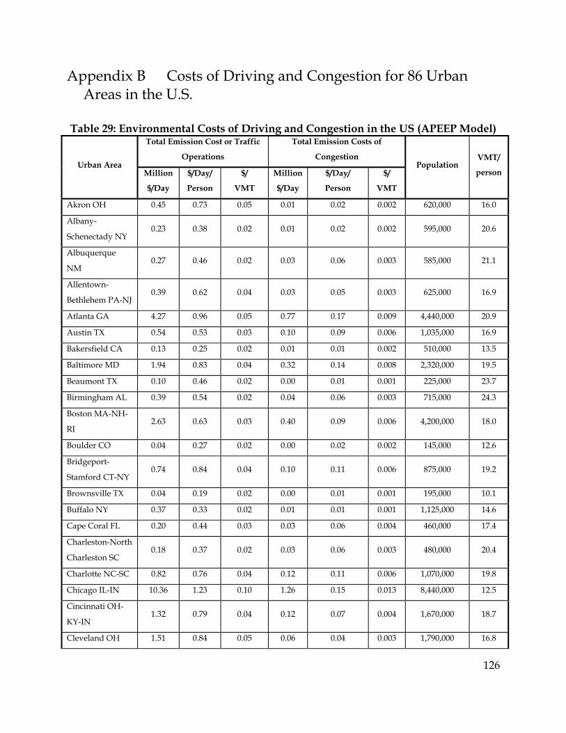
126

Appendix B Costs of Driving and Congestion for 86 Urban Areas in the U.S.

Table 29: Environmental Costs of Driving and Congestion in the US (APEEP Model)

Urban Area

Total Emission Cost or Traffic

Operations

Total Emission Costs of

Congestion Population

VMT/

person Million

$/Day

$/Day/

Person

$/

VMT

Million

$/Day

$/Day/

Person

$/

VMT

Akron OH 0.45 0.73 0.05 0.01 0.02 0.002 620,000 16.0

Albany-

Schenectady NY 0.23 0.38 0.02 0.01 0.02 0.002 595,000 20.6

Albuquerque

NM 0.27 0.46 0.02 0.03 0.06 0.003 585,000 21.1

Allentown-

Bethlehem PA-NJ 0.39 0.62 0.04 0.03 0.05 0.003 625,000 16.9

Atlanta GA 4.27 0.96 0.05 0.77 0.17 0.009 4,440,000 20.9

Austin TX 0.54 0.53 0.03 0.10 0.09 0.006 1,035,000 16.9

Bakersfield CA 0.13 0.25 0.02 0.01 0.01 0.002 510,000 13.5

Baltimore MD 1.94 0.83 0.04 0.32 0.14 0.008 2,320,000 19.5

Beaumont TX 0.10 0.46 0.02 0.00 0.01 0.001 225,000 23.7

Birmingham AL 0.39 0.54 0.02 0.04 0.06 0.003 715,000 24.3

Boston MA-NH-

RI 2.63 0.63 0.03 0.40 0.09 0.006 4,200,000 18.0

Boulder CO 0.04 0.27 0.02 0.00 0.02 0.002 145,000 12.6

Bridgeport-

Stamford CT-NY 0.74 0.84 0.04 0.10 0.11 0.006 875,000 19.2

Brownsville TX 0.04 0.19 0.02 0.00 0.01 0.001 195,000 10.1

Buffalo NY 0.37 0.33 0.02 0.01 0.01 0.001 1,125,000 14.6

Cape Coral FL 0.20 0.44 0.03 0.03 0.06 0.004 460,000 17.4

Charleston-North

Charleston SC 0.18 0.37 0.02 0.03 0.06 0.003 480,000 20.4

Charlotte NC-SC 0.82 0.76 0.04 0.12 0.11 0.006 1,070,000 19.8

Chicago IL-IN 10.36 1.23 0.10 1.26 0.15 0.013 8,440,000 12.5

Cincinnati OH-

KY-IN 1.32 0.79 0.04 0.12 0.07 0.004 1,670,000 18.7

Cleveland OH 1.51 0.84 0.05 0.06 0.04 0.003 1,790,000 16.8

127

Colorado Springs

CO 0.18 0.35 0.02 0.01 0.03 0.002 510,000 18.2

Columbia SC 0.22 0.48 0.02 0.02 0.03 0.002 455,000 24.3

Columbus OH 0.95 0.78 0.04 0.10 0.08 0.005 1,225,000 20.7

Corpus Christi

TX 0.09 0.28 0.02 0.00 0.01 0.001 325,000 17.7

Dallas-Fort

Worth-Arlington

TX

4.22 0.95 0.04 0.72 0.16 0.008 4,445,000 22.8

Dayton OH 0.59 0.79 0.04 0.03 0.04 0.003 745,000 18.3

Denver-Aurora

CO 1.97 0.90 0.05 0.27 0.12 0.007 2,180,000 19.9

Detroit MI 3.93 0.97 0.05 0.56 0.14 0.007 4,050,000 21.3

El Paso TX-NM 0.28 0.41 0.02 0.02 0.03 0.002 700,000 16.6

Eugene OR 0.05 0.18 0.01 0.00 0.01 0.001 250,000 14.2

Fresno CA 0.22 0.34 0.02 0.02 0.03 0.002 640,000 16.0

Grand Rapids MI 0.38 0.63 0.03 0.02 0.04 0.002 600,000 22.8

Hartford CT 0.52 0.58 0.03 0.04 0.04 0.003 895,000 20.6

Houston TX 3.91 1.02 0.04 0.73 0.190 0.009 3,815,000 23.7

Indianapolis IN 0.98 0.92 0.04 0.11 0.11 0.005 1,070,000 23.5

Jacksonville FL 0.51 0.49 0.02 0.08 0.08 0.004 1,040,000 21.3

Kansas City MO-

KS 1.51 0.99 0.04 0.04 0.03 0.002 1,525,000 22.5

Knoxville TN 0.26 0.53 0.02 0.02 0.05 0.003 490,000 23.1

Laredo TX 0.03 0.14 0.01 0.00 0.01 0.002 220,000 12.0

Las Vegas NV 0.48 0.34 0.02 0.11 0.08 0.005 1,405,000 18.3

Little Rock AR 0.26 0.68 0.02 0.02 0.04 0.002 390,000 29.5

Los Angeles-

Long Beach-

Santa Ana CA

22.98 1.79 0.09 5.35 0.42 0.020 12,800,000 20.9

Louisville KY-IN 0.78 0.86 0.04 0.09 0.10 0.005 915,000 22.6

Memphis TN-

MS-AR 0.66 0.64 0.03 0.05 0.05 0.003 1,035,000 21.5

Miami FL 3.42 0.63 0.04 0.71 0.13 0.008 5,420,000 17.2

Milwaukee WI 1.38 0.94 0.05 0.09 0.06 0.004 1,465,000 17.5

Minneapolis-St. 3.81 1.51 0.07 0.44 0.17 0.009 2,525,000 20.9

128

Paul MN

Nashville-

Davidson TN 0.63 0.64 0.02 0.06 0.06 0.003 995,000 26.2

New Haven CT 0.37 0.66 0.03 0.02 0.04 0.003 560,000 21.1

New Orleans LA 0.31 0.28 0.02 0.03 0.03 0.003 1,100,000 12.3

New York-

Newark NY-NJ-

CT

22.80 1.25 0.10 4.37 0.24 0.020 18,225,000 12.2

Oklahoma City

OK 0.60 0.68 0.03 0.04 0.05 0.002 875,000 25.1

Omaha NE-IA 0.33 0.51 0.03 0.03 0.05 0.003 645,000 17.3

Orlando FL 1.39 0.99 0.05 0.24 0.17 0.008 1,405,000 21.7

Oxnard-Ventura

CA 0.34 0.50 0.03 0.06 0.08 0.005 685,000 19.6

Pensacola FL-AL 0.14 0.39 0.02 0.02 0.04 0.003 355,000 20.8

Philadelphia PA-

NJ-DE-MD 4.88 0.92 0.06 0.69 0.13 0.009 5,310,000 15.9

Phoenix AZ 2.24 0.65 0.03 0.39 0.11 0.006 3,425,000 18.8

Pittsburgh PA 1.14 0.63 0.04 0.04 0.02 0.002 1,815,000 16.4

Portland OR-WA 0.64 0.35 0.02 0.13 0.07 0.005 1,800,000 15.2

Poughkeepsie-

Newburgh NY 0.30 0.59 0.03 0.02 0.03 0.002 515,000 19.5

Providence RI-

MA 0.65 0.52 0.03 0.06 0.05 0.003 1,245,000 18.4

Raleigh-Durham

NC 0.77 0.75 0.03 0.08 0.08 0.004 1,025,000 23.1

Richmond VA 0.54 0.58 0.02 0.03 0.03 0.002 935,000 23.4

Riverside-San

Bernardino CA 0.94 0.46 0.03 0.23 0.11 0.007 2,030,000 18.3

Rochester NY 0.22 0.30 0.02 0.01 0.01 0.001 745,000 15.5

Sacramento CA 1.27 0.68 0.04 0.23 0.13 0.008 1,860,000 16.2

Salem OR 0.07 0.31 0.02 0.01 0.02 0.002 230,000 15.7

Salt Lake City UT 0.52 0.53 0.03 0.06 0.06 0.004 975,000 16.6

San Antonio TX 0.83 0.57 0.03 0.13 0.09 0.005 1,450,000 21.0

San Diego CA 2.60 0.88 0.04 0.55 0.19 0.010 2,950,000 20.6

San Francisco- 4.51 1.01 0.06 0.95 0.21 0.012 4,480,000 18.0

129

Oakland CA

San Jose CA 1.37 0.80 0.04 0.27 0.16 0.009 1,705,000 19.8

Sarasota-

Bradenton FL 0.32 0.48 0.03 0.04 0.06 0.005 665,000 13.7

Seattle WA 1.57 0.51 0.03 0.29 0.09 0.005 3,100,000 18.6

Spokane WA 0.09 0.24 0.01 0.00 0.01 0.001 365,000 18.2

Springfield MA-

CT 0.24 0.37 0.02 0.01 0.01 0.001 660,000 17.2

St. Louis MO-IL 2.17 0.98 0.05 0.13 0.06 0.003 2,215,000 21.6

Tampa-St.

Petersburg FL 2.28 0.98 0.05 0.37 0.16 0.009 2,320,000 18.5

Toledo OH-MI 0.26 0.50 0.03 0.01 0.02 0.002 520,000 17.1

Tucson AZ 0.30 0.38 0.02 0.06 0.07 0.004 775,000 19.0

Tulsa OK 0.52 0.64 0.03 0.03 0.03 0.002 810,000 21.5

Virginia B.VA 0.62 0.40 0.02 0.09 0.06 0.003 1,545,000 18.7

Washington DC-

VA-MD 4.61 1.07 0.06 0.87 0.20 0.011 4,330,000 18.6

Wichita KS 0.20 0.43 0.02 0.00 0.00 0.001 455,000 21.0

Total 145.0 24 158355000

Average 1.7 0.64 0.03 0 0.1 0.005 1841337 19

Max 23.0 1.79 0.10 5 0.4 0.020 18225000 30

Min 0.03 0.14 0.01 0.002 0.004 0.001 145000 10

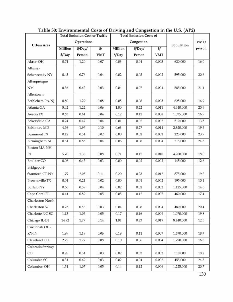
130

Table 30: Environmental Costs of Driving and Congestion in the U.S. (AP2)

Urban Area

Total Emission Cost or Traffic

Operations

Total Emission Costs of

Congestion Population

VMT/

person Million

$/Day

$/Day/

Person

$/

VMT

Million

$/Day

$/Day/

Person

$/

VMT

Akron OH 0.74 1.20 0.07 0.03 0.04 0.003 620,000 16.0

Albany-

Schenectady NY 0.45 0.76 0.04 0.02 0.03 0.002 595,000 20.6

Albuquerque

NM 0.36 0.62 0.03 0.04 0.07 0.004 585,000 21.1

Allentown-

Bethlehem PA-NJ 0.80 1.29 0.08 0.05 0.08 0.005 625,000 16.9

Atlanta GA 5.42 1.22 0.06 1.00 0.22 0.011 4,440,000 20.9

Austin TX 0.63 0.61 0.04 0.12 0.12 0.008 1,035,000 16.9

Bakersfield CA 0.24 0.47 0.04 0.01 0.02 0.002 510,000 13.5

Baltimore MD 4.56 1.97 0.10 0.63 0.27 0.014 2,320,000 19.5

Beaumont TX 0.12 0.54 0.02 0.00 0.02 0.001 225,000 23.7

Birmingham AL 0.61 0.85 0.04 0.06 0.08 0.004 715,000 24.3

Boston MA-NH-

RI 5.70 1.36 0.08 0.71 0.17 0.010 4,200,000 18.0

Boulder CO 0.06 0.43 0.03 0.00 0.02 0.002 145,000 12.6

Bridgeport-

Stamford CT-NY 1.79 2.05 0.11 0.20 0.23 0.012 875,000 19.2

Brownsville TX 0.04 0.21 0.02 0.00 0.01 0.002 195,000 10.1

Buffalo NY 0.66 0.59 0.04 0.02 0.02 0.002 1,125,000 14.6

Cape Coral FL 0.41 0.89 0.05 0.05 0.12 0.007 460,000 17.4

Charleston-North

Charleston SC 0.25 0.53 0.03 0.04 0.08 0.004 480,000 20.4

Charlotte NC-SC 1.13 1.05 0.05 0.17 0.16 0.009 1,070,000 19.8

Chicago IL-IN 14.92 1.77 0.14 1.91 0.23 0.019 8,440,000 12.5

Cincinnati OH-

KY-IN 1.99 1.19 0.06 0.19 0.11 0.007 1,670,000 18.7

Cleveland OH 2.27 1.27 0.08 0.10 0.06 0.004 1,790,000 16.8

Colorado Springs

CO 0.28 0.54 0.03 0.02 0.03 0.002 510,000 18.2

Columbia SC 0.31 0.69 0.03 0.02 0.04 0.002 455,000 24.3

Columbus OH 1.31 1.07 0.05 0.14 0.12 0.006 1,225,000 20.7

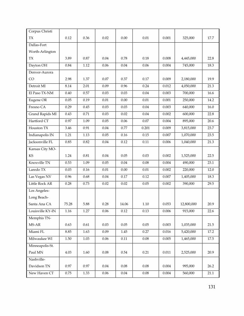
131

Corpus Christi

TX 0.12 0.36 0.02 0.00 0.01 0.001 325,000 17.7

Dallas-Fort

Worth-Arlington

TX 3.89 0.87 0.04 0.78 0.18 0.008 4,445,000 22.8

Dayton OH 0.84 1.12 0.06 0.04 0.06 0.004 745,000 18.3

Denver-Aurora

CO 2.98 1.37 0.07 0.37 0.17 0.009 2,180,000 19.9

Detroit MI 8.14 2.01 0.09 0.96 0.24 0.012 4,050,000 21.3

El Paso TX-NM 0.40 0.57 0.03 0.03 0.04 0.003 700,000 16.6

Eugene OR 0.05 0.19 0.01 0.00 0.01 0.001 250,000 14.2

Fresno CA 0.29 0.45 0.03 0.03 0.04 0.003 640,000 16.0

Grand Rapids MI 0.43 0.71 0.03 0.02 0.04 0.002 600,000 22.8

Hartford CT 0.97 1.09 0.05 0.06 0.07 0.004 895,000 20.6

Houston TX 3.46 0.91 0.04 0.77 0.201 0.009 3,815,000 23.7

Indianapolis IN 1.21 1.13 0.05 0.16 0.15 0.007 1,070,000 23.5

Jacksonville FL 0.85 0.82 0.04 0.12 0.11 0.006 1,040,000 21.3

Kansas City MO-

KS 1.24 0.81 0.04 0.05 0.03 0.002 1,525,000 22.5

Knoxville TN 0.53 1.09 0.05 0.04 0.08 0.004 490,000 23.1

Laredo TX 0.03 0.16 0.01 0.00 0.01 0.002 220,000 12.0

Las Vegas NV 0.96 0.68 0.04 0.17 0.12 0.007 1,405,000 18.3

Little Rock AR 0.28 0.73 0.02 0.02 0.05 0.002 390,000 29.5

Los Angeles-

Long Beach-

Santa Ana CA 75.28 5.88 0.28 14.06 1.10 0.053 12,800,000 20.9

Louisville KY-IN 1.16 1.27 0.06 0.12 0.13 0.006 915,000 22.6

Memphis TN-

MS-AR 0.63 0.61 0.03 0.05 0.05 0.003 1,035,000 21.5

Miami FL 8.85 1.63 0.09 1.45 0.27 0.016 5,420,000 17.2

Milwaukee WI 1.50 1.03 0.06 0.11 0.08 0.005 1,465,000 17.5

Minneapolis-St.

Paul MN 4.03 1.60 0.08 0.54 0.21 0.011 2,525,000 20.9

Nashville-

Davidson TN 0.97 0.97 0.04 0.08 0.08 0.004 995,000 26.2

New Haven CT 0.75 1.33 0.06 0.04 0.08 0.004 560,000 21.1

132

New Orleans LA 0.56 0.51 0.04 0.05 0.05 0.004 1,100,000 12.3

New York-

Newark NY-NJ-

CT 58.65 3.22 0.26 7.76 0.43 0.036 18,225,000 12.2

Oklahoma City

OK 0.66 0.76 0.03 0.05 0.06 0.003 875,000 25.1

Omaha NE-IA 0.37 0.58 0.03 0.04 0.06 0.004 645,000 17.3

Orlando FL 3.05 2.17 0.10 0.41 0.29 0.014 1,405,000 21.7

Oxnard-Ventura

CA 0.70 1.03 0.05 0.09 0.14 0.008 685,000 19.6

Pensacola FL-AL 0.26 0.73 0.04 0.02 0.06 0.004 355,000 20.8

Philadelphia PA-

NJ-DE-MD 11.31 2.13 0.13 1.36 0.26 0.017 5,310,000 15.9

Phoenix AZ 2.73 0.80 0.04 0.51 0.15 0.008 3,425,000 18.8

Pittsburgh PA 2.18 1.20 0.07 0.07 0.04 0.003 1,815,000 16.4

Portland OR-WA 0.84 0.47 0.03 0.18 0.10 0.007 1,800,000 15.2

Poughkeepsie-

Newburgh NY 0.60 1.17 0.06 0.02 0.05 0.003 515,000 19.5

Providence RI-

MA 1.46 1.18 0.06 0.11 0.09 0.005 1,245,000 18.4

Raleigh-Durham

NC 0.96 0.94 0.04 0.11 0.10 0.005 1,025,000 23.1

Richmond VA 0.78 0.83 0.04 0.04 0.04 0.002 935,000 23.4

Riverside-San

Bernardino CA 2.11 1.04 0.06 0.41 0.20 0.012 2,030,000 18.3

Rochester NY 0.32 0.43 0.03 0.01 0.01 0.001 745,000 15.5

Sacramento CA 1.56 0.84 0.05 0.31 0.17 0.011 1,860,000 16.2

Salem OR 0.09 0.39 0.02 0.01 0.03 0.002 230,000 15.7

Salt Lake City UT 0.89 0.91 0.05 0.08 0.08 0.006 975,000 16.6

San Antonio TX 0.87 0.60 0.03 0.15 0.11 0.006 1,450,000 21.0

San Diego CA 8.19 2.78 0.14 1.39 0.47 0.023 2,950,000 20.6

San Francisco-

Oakland CA 12.59 2.81 0.16 2.19 0.49 0.028 4,480,000 18.0

San Jose CA 2.88 1.69 0.09 0.48 0.28 0.015 1,705,000 19.8

Sarasota-

Bradenton FL 0.60 0.90 0.07 0.08 0.12 0.009 665,000 13.7

133

Seattle WA 3.52 1.13 0.06 0.48 0.16 0.009 3,100,000 18.6

Spokane WA 0.12 0.32 0.02 0.00 0.01 0.001 365,000 18.2

Springfield MA-

CT 0.55 0.83 0.05 0.02 0.02 0.002 660,000 17.2

St. Louis MO-IL 2.11 0.95 0.04 0.14 0.06 0.003 2,215,000 21.6

Tampa-St.

Petersburg FL 4.74 2.04 0.11 0.66 0.28 0.016 2,320,000 18.5

Toledo OH-MI 0.37 0.71 0.04 0.02 0.03 0.002 520,000 17.1

Tucson AZ 0.38 0.50 0.03 0.07 0.09 0.005 775,000 19.0

Tulsa OK 0.51 0.62 0.03 0.03 0.03 0.002 810,000 21.5

Virginia B.VA 1.02 0.66 0.04 0.12 0.08 0.005 1,545,000 18.7

Washington DC-

VA-MD 7.76 1.79 0.10 1.33 0.31 0.017 4,330,000 18.6

Wichita KS 0.22 0.48 0.02 0.00 0.00 0.001 455,000 21.0

Total 301 44.5 158,355,000

Average 4 1.1 0.06 0.5 0.13 0.01 1,841,337 19

Max 75 5.9 0.3 14.1 1.10 0.05 18,225,000 30

Min 0.03 0.2 0.01 0.002 0.005 0.001 145,000 10

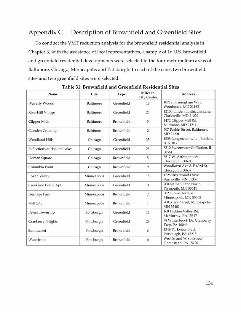
134

Appendix C Description of Brownfield and Greenfield Sites

To conduct the VMT reduction analysis for the brownfield residential analysis in

Chapter 3, with the assistance of local representatives, a sample of 16 U.S. brownfield

and greenfield residential developments were selected in the four metropolitan areas of

Baltimore, Chicago, Minneapolis and Pittsburgh. In each of the cities two brownfield

sites and two greenfield sites were selected.

Table 31: Brownfield and Greenfield Residential Sites Name City Type Miles to

City Center Address

Waverly Woods Baltimore Greenfield 18 10712 Birmingham Way, Woodstock, MD 21163

RiverHill Village Baltimore Greenfield 24 12100 Linden Linthicum Lane, Clarksville, MD 21029

Clipper Mills Baltimore Brownfield 3 1472 Clipper Mill Rd, Baltimore, MD 21211

Camden Crossing Baltimore Brownfield 2 307 Parkin Street, Baltimore, MD 21201

Woodland Hills Chicago Greenfield 35 1538 Longmeadow Ln, Bartlett, IL 60103

Reflections at Hidden Lakes Chicago Greenfield 25 8310 Sweetwater Ct, Darien, IL 60561

Homan Square Chicago Brownfield 5 3517 W. Arthington St, Chicago, IL 60624

Columbia Point Chicago Brownfield 9 Woodlawn Ave & E 63rd St, Chicago, IL 60637

Itokah Valley Minneapolis Greenfield 18 1725 Riverwood Drive, Burnsville, MN 55337

Creekside Estate Apt. Minneapolis Greenfield 9 200 Nathan Lane North, Plymouth, MN 55441

Heritage Park Minneapolis Brownfield 2 502 Girard Terrace, Minneapolis, MN 55405

Mill City Minneapolis Brownfield 1 700 S. 2nd Street, Minneapolis, MN 55401

Peters Township Pittsburgh Greenfield 14 168 Hidden Valley Rd, McMurray, PA 15317

Cranberry Heights Pittsburgh Greenfield 28 78 Winterbrook Dr, Cranberry Twp, PA 16066

Summerset Pittsburgh Brownfield 6 1346 Parkview Blvd, Pittsburgh, PA 15215

Waterfront Pittsburgh Brownfield 6 West St and W 8th Street, Homestead, PA 15120

135

Appendix D Travel Demand Modeling7

Travel demand models (TDM) replicate real world travel patterns. A TDM takes into

account travel behaviors that influence drivers’ choice of destination, mode of

transportation and selected routes [68]. TDMs typically include a four-step process:

Trip generation estimates the number of trips produced by household and attracted

by other places of employment, shopping and recreation. Information from land use,

population and economic forecasts are used to estimate trip generation. Trip

generations are estimated by purpose: home-based work trip, home-based non-work

trips, non-home-based trips as well as truck trips and taxi trips. Home-based work trips

are based on household characteristics such as the number of people in the household

and the number of vehicles available.

Trip distribution distributes trips generated to specific origin and destination

movements. Trips found by the first step, trip generation, are linked together to shape

an origin-distribution table. Gravity model is the most popular way to calculate origin-

distribution tables. The model distributes trips produced by one zone to other zones

based on the size and distance of the zones.

Mode split estimates the mode of travel used and it share for each trip. Mode split

calculations are estimated with Logit Models which involves a comparison of travel

between two points by various available modes using a combination of cost, travel time

and a mode between an origin and a destination. In this step of the model automobile

trips are converted from person trips to vehicle trips based on auto occupancy factors.

Traffic assignment which finds the specific path different modes take from an origin

to a destination. Trips from an origin to a destination are first assigned using the

shortest path (minimum time path). Then all assigned trips are added up and are

matched again the capacity of the roadway. If the roadway is congested then the speed

gets adjusted and that increases the original shortest time path. So the whole process

7 TDM information from Southern California Association of Governments: http://www.scag.ca.gov/modeling/dmp.htm#a 

136

goes through iterations to find equilibrium between demand and supply in the

transportation network. Time of day is an important factor in the traffic assignment

portion of TDM. For this study four metropolitan planning organizations were

providing data on their Travel Demand Models:

Southwestern Pennsylvania Commission (SPC)8: SPC is the metropolitan planning

organization in charge of Pittsburgh and 10 counties in the southwestern Pennsylvania

region. SPC in responsible for short term and long term transportation plans within the

region. For their TDM SPC uses TP+ modeling software package. The method used is

the four step process9.

Minneapolis/St. Paul Metropolitan Council10: The Metropolitan Council is the

regional planning agency responsible for the short term and long term transportation

plans within Twin Cities 7 counties. For the TDM, SPC uses TP+ modeling software

package. The method used is the four step process11.

Chicago Metropolitan Agency for Planning (CMAP)12: CMAP is the regional planning

organization responsible for 7 northeastern Illinois counties. For the their TDM, CMAP

uses EMME/2 modeling software 13.

Baltimore Metropolitan Council14: The Baltimore Metropolitan Council is

responsible for the short term and long term transportation plans of Baltimore City and

five other counties. For their TDM, the Baltimore Metropolitan Council uses the

Cube/TP+ modeling software package15.

8 http://www.spcregion.org/ 9 Detailed information on SPC’s travel estimation process (part of the conformity report) is available at: http://www.spcregion.org/pdf/AQ11‐14/Conformity_Sec%20IV_FinalReport_July‐10.pdf 10 http://www.metrocouncil.org/ 11 Detailed information on the Metropolitan Council’s travel demand process is available at: http://www.metrocouncil.org/planning/transportation/TIP/tip2009_2013.pdf  12 http://www.cmap.illinois.gov/ 13 Detailed information on CMAP’s travel demand process is available at: http://www.cmap.illinois.gov/technical‐reports 14 http://www.baltometro.org/ 15 Detailed information on the Baltimore Metropolitan Council’s travel demand process is available at: http://www.baltometro.org/reports/CalibrationReport.pdf 

137

Appendix E Retail Stores Information

REI

412 S. 27th Street,

Pittsburgh, PA

15203

600 Settlers Ridge

Center Drive,

Pittsburgh, PA

15205

Costco

501 W Waterfront

Dr.

West Homestead

PA 15120-5009

1050 Cranberry

Square Drive,

Cranberry

Township, PA

16066

202 Costco Drive,

Pittsburgh PA

15205

Giant

Eagle

420 East

Waterfront Drive,

Homestead, PA

15210

4250 Murray

Avenue,

Pittsburgh, PA

15217

1705 South

Braddock

Avenue

Pittsburgh, PA

15218

254 Yost

Boulevard-

Braddock

Pittsburgh, PA

15221

1356 Hoffman

Boulevard

West Mifflin, PA

15122

600 Towne

Square Way

Pittsburgh, PA

15227

Target

6231 Penn

Avenue,

Pittsburgh, PA

15206

4004 Monroeville

Blvd

Monroeville, PA

15146

600 Chauvet Dr.

North Fayette,

PA

15275

1717 Lebanon

Church Road, West

Mifflin

15122

2661 Freeport

Road,

Pittsburgh, PA

15238

4801 McKnight

Road #3,

Pittsburgh, PA

15237

360 East

Waterfront

Drive,

Homestead

15120

Brownfield/Infill

Locations

138

Appendix F Traffic Signal Timing Terminology

Cycle Length

The time (in seconds) required for one complete sequence of signal indications.

Offset

The time relationship between coordinated phases defined reference point and a

defined master reference (master clock or sync pulse).

Phase

A timing unit associated with the control of one or more indications. A phase may be

timed considering complex criteria for determination of sequence and the duration of

intervals.

Coordination

The ability to synchronize multiple intersections to enhance the operation of one or

more directional movements in a system.

Controller

The devices that physically operate the signal timing controls, including the controller,

detectors, signal heads, and conflict monitor.

ASC/3 Series NEMA TS2 Controllers

Traffic signal controller manufactured by Econolite16 that combines the requirements of

NEMA TS2 operation with the actual controller.

Aries Closed Loop Operating System

A Windows based data management and monitoring system for arterial control systems

manufactured by Econolite16.

Centracs

Centralized advanced management system manufactured by Econolite16.

16 www.econolite.com 

139

Appendix G Cranberry Township Vehicular Counts

Route 19 & Rowan Road 

Time     NL  NT  NR  SL   ST   SR  EL  ET  ER  WL  WT  WR 

AM 

Old  265  595  185  65  919  10  10  45  45  350  85  110 

New  186  422  152  73  770  17  18  49  14  334  59  140 

% change  ‐30  ‐29  ‐18  12  ‐16  70  80  9  ‐69  ‐5  ‐31  27 

Midday 

Old  185  885  330  100  880  15  15  45  85  305  45  65 

New  141  806  311  76  748  13  23  65  160  353  35  92 

% change  ‐31  ‐10  ‐6  ‐32  ‐18  ‐15  35  31  47  14  ‐29  29 

PM 

Old  135  1273  495  120  905  5  55  100  185  375  60  145 

New  146  1108  507  140  836  19  53  110  186  466  56  157 

% change  8  ‐15  2  14  ‐8  74  ‐4  9  1  20  ‐7  8 

Route 19 & Rochester Road 

Time     NL  NT  NR  SL   ST   SR  EL  ET  ER  WL  WT  WR 

AM 

Old  130  795  10  45  1094  375  405  20  285  25  10  20 

New  174  855  21  40  1008  401  432  31  319  37  13  16 

% change  34  8  110  ‐11  ‐8  7  7  55  12  48  30  ‐20 

Midday 

Old  265  1055  80  75  1020  305  395  30  265  95  35  80 

New  276  924  128  75  758  316  359  41  271  105  67  115 

% change  4  ‐14  38  0  ‐35  3  ‐10  27  2  10  48  30 

PM 

Old  410  1398  70  35  1380  570  575  30  325  60  30  85 

New  411  709  73  87  978  591  579  33  343  53  55  69 

% change  0  ‐97  4  60  ‐41  4  1  9  5  ‐13  45  ‐23 

Route 19 & Freeport Road 

Time     NL  NT  NR  SL   ST   SR  EL  ET  ER  WL  WT  WR 

AM 

Old  70  835  140  110  1244  25  95  20  40  230  20  55 

New  108  607  77  55  1040  22  82  14  27  199  10  59 

% change  54  ‐27  ‐45  ‐50  ‐16  ‐12  ‐14  ‐30  ‐33  ‐13  ‐50  7 

140

Midday 

Old  125  1060  115  120  1030  60  220  45  85  165  20  75 

New  233  1060  237  163  893  62  166  33  83  211  26  100 

% change  46  0  51  26  ‐15  3  ‐33  ‐36  ‐2  22  23  25 

PM 

Old  120  1605  390  170  1184  50  170  45  50  190  20  95 

New  172  1458  293  130  972  11  150  44  74  183  32  147 

% change  30  ‐10  ‐33  ‐31  ‐22  ‐355 ‐13  ‐2  32  ‐4  38  35 

 

 

Route 19 & Freedom Road 

Time     NL  NT  NR  SL   ST   SR  EL  ET  ER  WL  WT  WR 

AM 

Old  385  725  334  546  545  70  75  499  245  330  530  140 

New  411  852  275  563  709  100  108  516  304  411  588  196 

% change  7  18  ‐18  3  30  43  44  3  24  25  11  40 

Midday 

Old  340  835  435  710  830  120  185  505  235  360  420  240 

New  266  879  427  623  780  128  209  464  230  388  498  276 

% change  ‐28  5  ‐2  ‐14  ‐6  6  11  ‐9  ‐2  7  16  13 

PM 

Old  415  955  420  730  890  110  175  630  315  424  485  263 

New  443  1005  358  683  824  142  170  579  245  303  568  253 

% change  6  5  ‐17  ‐7  ‐8  23  ‐3  ‐9  ‐29  ‐40  15  ‐4 

Route 19 & Brandt Road 

Time     NL  NT  NR  SL   ST   SR  EL  ET  ER  WL  WT  WR 

AM 

Old  30  745  5  55  1306  20  5  5  10  5  10  290 

New  7  517  0  39  1342  2  13  5  1  1  6  186 

% change  ‐77  ‐31  ‐100 ‐29  3  ‐90  160  0  ‐90  ‐80  ‐40  ‐36 

Midday 

Old  75  1060  20  55  1306  20  55  5  70  20  25  450 

New  45  952  11  111  1192  73  41  5  64  19  15  372 

% change  ‐67  ‐11  ‐82  50  ‐10  73  ‐34  0  ‐9  ‐5  ‐67  ‐21 

PM Old  40  1308  15  70  1245  75  95  5  45  15  25  615 

New  41  1223  13  104  1323  46  65  3  54  15  20  522 

141

% change  2  ‐7  ‐15  33  6  ‐63  ‐46  ‐67  17  0  ‐25  ‐18 

Freedom & Haine 

Time     NL  NT  NR  SL   ST   SR  EL  ET  ER  WL  WT  WR 

AM 

Old  10  30  20  240  50  25  50  904  15  5  250  30 

New  12  52  22  276  56  57  105  816  11  13  325  61 

% change  20  73  10  15  12  128  110  ‐10  ‐27  160  30  103 

Midday 

Old  10  25  20  140  30  45  45  490  10  15  530  110 

New  10  29  12  199  33  63  56  470  9  24  506  91 

% change  0  14  ‐67  30  9  29  20  ‐4  ‐11  38  ‐5  ‐21 

PM 

Old  75  105  15  120  55  55  70  510  10  25  805  250 

New  53  129  22  136  47  106  130  216  22  29  792  242 

% change  ‐42  19  32  12  ‐17  48  46  ‐136  55  14  ‐2  ‐3 

 

 

 

 

 

Freedom & Executive 

Time     NL  NT  NR  SL   ST   SR  EL  ET  ER  WL  WT  WR 

AM 

Old  5  1  1  135  10  175  100  769  5  1  645  170 

New  6  5  1  153  4  173  114  828  7  2  760  192 

% change  20  400  0  13  ‐60  ‐1  14  8  40  100  18  13 

Midday 

Old  20  15  5  242  20  275  240  795  40  0  780  265 

New  18  19  4  203  25  302  192  584  21  8  587  265 

% change  ‐11  21  ‐25  ‐19  20  9  ‐25  ‐36  ‐90  100  ‐33  0 

PM 

Old  40  10  0  240  25  290  235  870  30  0  870  240 

New  21  10  3  212  12  218  1  426  264  221  1  15 

% change  ‐90  0  100  ‐13  ‐108  ‐33  ‐23400  ‐104  89  100  0  ‐1500 

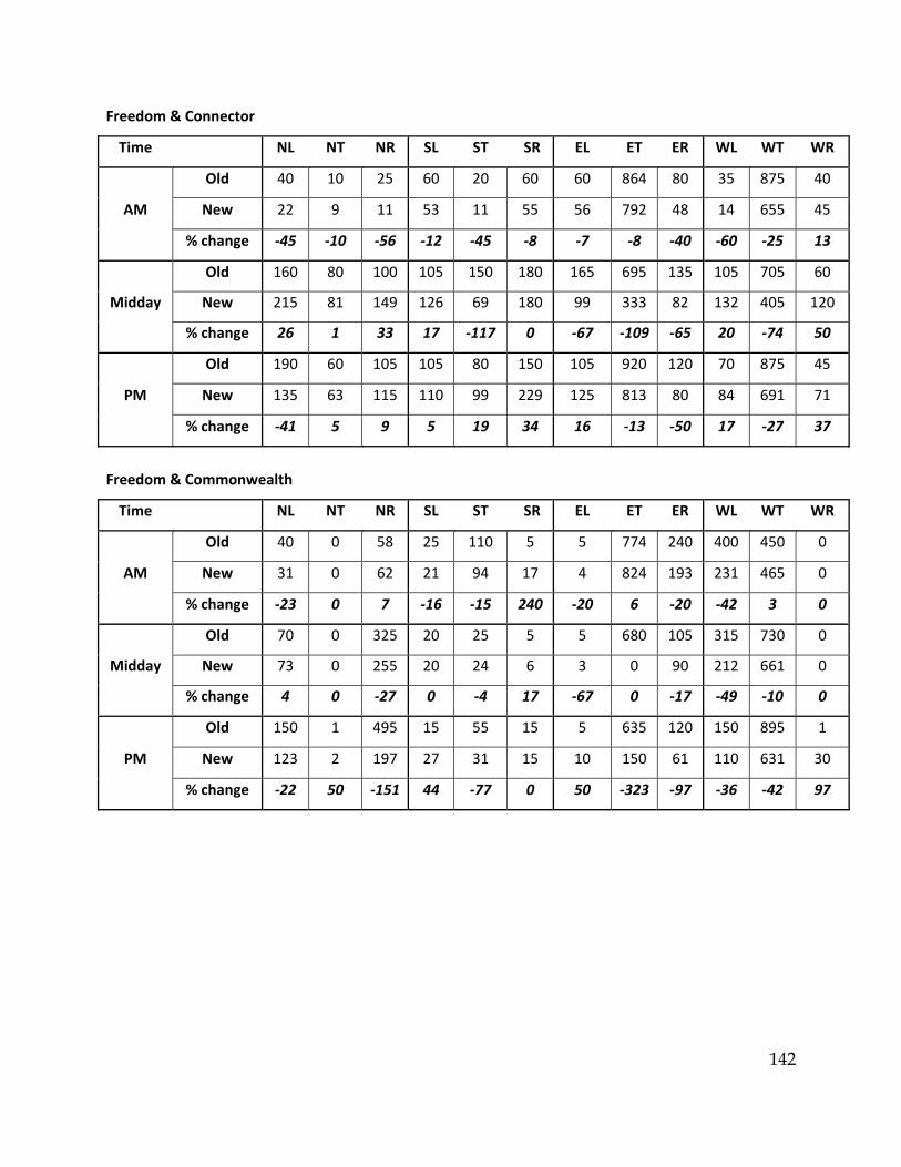
142

Freedom & Connector 

Time     NL  NT  NR  SL   ST   SR  EL  ET  ER  WL  WT  WR 

AM 

Old  40  10  25  60  20  60  60  864  80  35  875  40 

New  22  9  11  53  11  55  56  792  48  14  655  45 

% change  ‐45  ‐10  ‐56  ‐12  ‐45  ‐8  ‐7  ‐8  ‐40  ‐60  ‐25  13 

Midday 

Old  160  80  100  105  150  180  165  695  135  105  705  60 

New  215  81  149  126  69  180  99  333  82  132  405  120 

% change  26  1  33  17  ‐117  0  ‐67  ‐109  ‐65  20  ‐74  50 

PM 

Old  190  60  105  105  80  150  105  920  120  70  875  45 

New  135  63  115  110  99  229  125  813  80  84  691  71 

% change  ‐41  5  9  5  19  34  16  ‐13  ‐50  17  ‐27  37 

Freedom & Commonwealth 

Time     NL  NT  NR  SL   ST   SR  EL  ET  ER  WL  WT  WR 

AM 

Old  40  0  58  25  110  5  5  774  240  400  450  0 

New  31  0  62  21  94  17  4  824  193  231  465  0 

% change  ‐23  0  7  ‐16  ‐15  240  ‐20  6  ‐20  ‐42  3  0 

Midday 

Old  70  0  325  20  25  5  5  680  105  315  730  0 

New  73  0  255  20  24  6  3  0  90  212  661  0 

% change  4  0  ‐27  0  ‐4  17  ‐67  0  ‐17  ‐49  ‐10  0 

PM 

Old  150  1  495  15  55  15  5  635  120  150  895  1 

New  123  2  197  27  31  15  10  150  61  110  631  30 

% change  ‐22  50  ‐151 44  ‐77  0  50  ‐323  ‐97  ‐36  ‐42  97