Assessment of groundwater mass balance and zone budget …

Assessment of groundwater mass balance and zonebudget in the semi-arid region: A case study ofPalar sub-basin, Tamil Nadu, India

MATHIAZHAGAN MOOKIAH* , SANJEEV KUMAR JHA and ASHIS BISWAS

Earth and Environmental Sciences, Indian Institute of Science Education and Research, Bhopal, India.*Corresponding author. e-mail: [email protected]

MS received 21 September 2020; revised 11 May 2021; accepted 20 May 2021

The assessment of groundwater potential zones is crucial for estimating and managing availablegroundwater resources. In the proposed study, quantiBcation of groundwater availability is performedusing the information collected from the hydrogeological and geophysical (electrical resistivity) investi-gation of the aquifer. We delineate groundwater potential zones using a weighted overlay analysis basedon the conventional method with 110 electrical resistivity surveys and 40 lithological data. MODFLOW isused to calibrate and validate the Cow pattern and groundwater characteristics. The study area comprisesa complex geological formation. The groundwater potential map is prepared using the observedgroundwater level instead of rainfall data as the study area lacks rainfall stations. The Bnal potential mapis validated with the speciBc capacity obtained from the pumping test. This map is divided into 13 zonesand each zone is considered as boundaries for the MODFLOW simulation. The thickness of each zone isassessed using the electrical resistivity method. The calibration and validation of the groundwater modelare performed for one year and 1.5 years, respectively, between November 2012 and March 2015. Weconsider two layers, namely topsoil and unconBned/semi-conBned aquifers in the groundwater model.During the calibration and validation periods, the groundwater volume is found to be 7.12 and 7.51 Mm3,respectively. The groundwater mass balance assessment performed in this study will be helpful in theplanning and management of groundwater resources in the area.

Keywords. Groundwater potential zone; visual MODFLOW; groundwater velocity; electricalresistivity; mass balance.

1. Introduction

In recent years, the depletion of groundwater hasbecome an alarming issue in many countries. Thecontinuous lowering of the groundwater table isattributed to various factors, such as climatechange, rapid urbanization, industrialization, andchanges in land cover and land-use patterns(Mukherjee et al. 2018; Patra et al. 2018). Thedemand for groundwater is increasing every year

due to the growing population, irrigation needs,urbanization, and the recurrence of drought(Panda et al. 2007; Gupta et al. 2011; Halder et al.2020). A major population of rural areas in India isdependent on groundwater for drinking anddomestic uses. The groundwater investigations inIndia are mainly conBned to the unconsolidatedalluvial and semi-consolidated sedimentary areas.However, nearly 70% of peninsular India isunderlain with hard rocks, and a large extent of

J. Earth Syst. Sci. (2021) 130:187 � Indian Academy of Scienceshttps://doi.org/10.1007/s12040-021-01691-2 (0123456789().,-volV)(0123456789().,-volV)

these areas does not have adequate informationabout subsurface water resources (CGWB 2012).The monitoring and managing of groundwater

resources is a complex task, as the associatedaquifers are vast and unexplored (Zektser andLorne 2004). Appropriate strategies are required toassess the groundwater potential of a region (Ku-mar et al. 2009; Dar et al. 2010; Oh et al. 2011). Inmost groundwater investigations, water qualityanalysis and pumping tests are carried out (Baueret al. 2004; Bahir et al. 2019). These results areoverlaid with meteorological, geological, andtopographical maps to delineate groundwaterpotential zones. Conducting these types of studiesis time-consuming, cumbersome, and Bnanciallyexpensive.Groundwater exploration is performed using

geophysical surveys, hydrogeological data, andremote sensing techniques. Geophysical surveysare essential, not only for identifying the potentialgroundwater zones but also for monitoring theperiodical changes in the availability of ground-water (Ahmed et al. 1988; Cassiani and Medina1997; Slater 2007; Mastrocicco et al. 2010). TheBeld-scale hydrogeological investigations, such asthe real-time monitoring of the groundwater levels,provide a more accurate estimation of groundwateravailability. However, such a monitoring approachis tedious and time-demanding. To this end,numerical models are used extensively for theproper management of groundwater resources.A groundwater model provides a framework to

conceptualize different hydrogeological processes(precipitation, inBltration, run-oA, evapotranspi-ration, etc.) and synthesize Beld observationsquantitatively. Numerical simulation is used todetermine the spatial and temporal distributions ofgroundwater recharge in an alluvial aquifer system(Liu et al. 2014; Jha et al. 2015). Hydrologic modelsare developed with MODFLOW to estimate therecent and historical uses of groundwater in thesemi-arid regions (Mart�ınez-Santos and Andreu2010; Falke et al. 2011) and to explore the propergroundwater management solutions in over-exploited regions (Candela et al. 2009; Zhang andHiscock 2010; Mikita et al. 2011; Li et al. 2013;Wang et al. 2015). Many researchers have usednumerical models to investigate the eAects ofoverexploitation of groundwater on its futureavailability and management (Palma and Bentley2007; Zume and Tarhule 2008; Pisinaras et al.2013; Jha et al. 2014). Numerical models have alsobeen coupled with GIS techniques to study the

behaviour of groundwater Cow in a hard rockaquifer to investigate the hydrological processes(Sekhar et al. 2004; Sashikkumar et al. 2017).This study aims to identify the productive and

proliBc aquifer in the study region. The outcomeof this study will guide the governmental andother national agencies by suggesting the potentialareas and depth of boreholes to be drilled forpotable water in the study region. The presentstudy focuses on the numerical simulation ofgroundwater using the Visual MODFLOW (ver-sion 4.6) model to integrate geophysical andhydrological survey data in a GIS environment.The main objectives of this study are: (i) to developa methodology to map the heterogeneity of theaquifer in order to delineate the groundwaterpotential zones, (ii) to apply an integratedapproach of combining geophysical method,groundwater quality analysis and pumping testdata in a GIS environment, and (iii) to estimate thequantity of groundwater in different regions using anumerical groundwater model and the developedgroundwater potential map.

2. Study area

The present study is conducted (Bgure 1) inWalajabad Block which is located between thegeographical coordinates of latitude 13�1401200 to12�1503800 and longitude 79�3003700 to 80�3004200with an estimated area of 325 km2. The Palar riveris the major river draining across the district,Cowing from west to east near the southernboundary. Since the Palar river is seasonal in nat-ure, groundwater is the primary source to meet thedrinking and irrigation demands of this area. Basedon the 2011 census, there were 40,143 householdswith a population of 161,524 in Walajabad Block.For household consumption, residents mainlydepend on wells and hand pumps.The geology of the Walajabad Block is primarily

made up of hard rocks and sedimentary formationsoverlaid by alluvium and clay. Figure 2(a and b)show the geology and land use map of the studyarea. Alluvium deposits are found in the northwestand southeast, while sandstone and granitic gneissoccur in the remaining part of the study area.Alluvial deposits are the youngest formation con-sisting of sand and clay deposited by the riverVagavathy and Palar. The Palar alluvium consistsof coarse sand and gravel. The average thickness ofalluvium ranges from 1 to 30 m. The sedimentary

187 of 18 J. Earth Syst. Sci. (2021) 130:187

formation consists of clay, shale, sandstone, andconglomerate. Shale and clay in the study area areof the upper Gondwana period. Sandstone is calledConjeevaram gravel and is similar to Cuddaloreand Rajmundry sandstones of the Tertiary periodthat occurs in some pockets. Around 30% of the

study area has hard rock having granite gneiss.Groundwater is mainly found under phreaticconditions in weathered, fractured, jointed andfaulted portions of granitic rocks and under arte-sian conditions in fractured zones situated belowimpervious hard rocks.

Figure 1. (a) Geographical location of the study area and (b) location of available data along with elevation map in thebackground.

Figure 2. (a) Geology and (b) land use map of Walajabad Block.

J. Earth Syst. Sci. (2021) 130:187 of 18 187

The climate of the study area is hot andsemi-arid. The annual maximum and minimumtemperatures of the study area are 37.10� and20.5�C, respectively. March, April, and Mayexperience high temperatures while November,December, and January experience low tem-peratures. The total annual rainfall recorded atthe nearest rain gauge station, located atAyyenkarkulam (Kancheepuram), is 1272 mm.The rainy season comprises the southwestmonsoon (June–September), northeast monsoon(October–December) and some transition per-iod. Heavy rainfalls during the northeast mon-soon occur due to depressions and stormsoccurring in the Bay of Bengal.

3. Data and methods

3.1 Description of dataset

Weather data: Monthly rainfall data of 2.5 yrs atAyyenkarkulam (Kanchipuram) rain gauge stationmonitored by the India Meteorology Department(IMD) was used for the analysis. Evapotranspira-tion data was collected from the Karunguzhistation.

Groundwater level data: To monitor the depthof groundwater level and collect samples for thechemical analysis, Bve observation wells monitoredby the government agencies namely, Tamil NaduPublic Works Department, Tamil Nadu WaterSupply and Drainage Board, and CentralGroundwater Board in Walajabad Block wereselected. Further, a network of 28 self-monitoredobservation wells spread over the entire study areawas established. The Cuctuation in groundwaterlevels was monitored monthly for the entire 2.5 yrs.Observations show that the groundwater level risesto the maximum level (2 m bgl) during the mon-soon and declines to the minimum (6 m bgl) duringsummer.

Groundwater chemistry: In January 2013,total dissolved solid (TDS) in groundwater wasmeasured in 28 open wells. Wells for TDS anal-ysis were selected as nearly as possible to thevertical electrical sounding (VES) points tocompare the electrical resistivity measured bythe geophysical method and the TDS. Ground-water samples from open wells were collectedusing a rinsed bucket from the depth up to 10 m.TDS was measured in the sample at the Beld

using the EQ 8361 EQUINOX pen-type EC/TDSprobe meter.

Slope calculation: The reduced level of thestudy area was assessed using a handheld GPS.The maximum and minimum (elevation) in thestudy area range from 100 to 45 m above meansea level. The elevation gradient is inclinedfrom northwest to southeast (see Bgure 1). Theslope map was prepared using the ArcGISSpatial Analyst Module from the DifferentialGPS (DGPS) data at 110 points collected fromthe Beld. The slope of the study area rangesfrom 0.2 to 0.4�, indicating that it has a gentleslope.

Lithological and electrical resistivity data:Forty lithological data were collected from theTamil Nadu Water Supply and Drainage Board toassess the detailed subsurface proBle of the Wala-jabad Block. Aquifer parameters (e.g., transmis-sivity, permeability, and speciBc capacity) werederived from the pumping test in 15 dug wells. Inthe context of this study, only the transmissivitywas considered essential and used in further anal-ysis. The electrical resistivity survey using ABEMSAS 1000 Terrameters, Sweden, was conducted at110 VES points. The sounding curves were inter-preted to determine the resistivity and thickness ofthe subsurface layers.The Dar–Zarrouk (DZ) analysis was also per-

formed for this study. The longitudinal conduc-tance, one of the DZ parameters, was consideredfor this study. It was derived (equation 1) from thelayer thickness (hi) and resistivity values (qi) usingthe following relation:

Longitudinal conductance Sð Þ ¼ hiqi

Siemensð Þ: ð1Þ

3.2 Interpolation and extrapolation of data

The success of any geophysical survey depends onthe validation with actual hydrogeological infor-mation. We used interpolation and extrapolationtechniques on geophysical outputs to determine thetype of subsurface formation and groundwaterresource potential zone of the entire study area.Linear regression was used to estimate the corre-lation between the DZ parameter (longitudinalconductance) and hydrogeological parameter(transmissivity). Subsequently, the thickness of alayer determined by the electrical resistivity data


was veriBed with the lithological data collectedfrom the existing 40 boreholes.The heterogeneity of the entire study area is

clearly indicated in the qualitative interpretation.Predominantly H-type and H-type mixturecurves exist in the study area except for hard rockterrain. The H-type curves are used to assess theareas of significant aquifers within the study area.A-type and A-type combination curves are foundin hard rock regions. The K-type and K-typecombination curves uncover the areas of theaquitard and the Q-type and Q-type combinationcurve shows the areas of the clay or salinity of thesubsurface aquifer. Quantitative interpretationindicates that most of the VES points in the studyarea have adequate aquifer thickness and waterholding capacity. The topsoil varies from 0.5 to 5m with an average of 1.7 m. The unconBnedaquifer ranges from 2.5 to 46 m with an average of10 m. The detailed qualitative and quantitativedetails are provided in Mathiazhagan et al.(2015).In addition, we correlated the electrical resis-

tivity values measured in geophysical surveys withthe measured TDS in the groundwater sample. Agood correlation was obtained between the trans-missivity and longitudinal conductance (R2 =0.856 in alluvium, 0.866 in sedimentary and 0.999in hard rock) and between the TDS and electricalresistivity (R2 = 0.936 in alluvium, 0.930 in

sedimentary and 0.901 in hard rock). Based onthese correlations, the longitudinal conductanceand electrical resistivity values were extrapolatedto obtain the transmissivity and TDS, respectively,to generate their spatial distribution map over thestudy area (Bgure 3a and b).

3.3 Multi-inCuencing factor

The methodology adopted in the present study isshown in a Cow chart in Bgure 4. For an integratedgroundwater investigation, aquifer parameters ofdifferent layers, groundwater level, slope, drainagepattern, land use, and lineaments are required.Nine inCuencing factors, i.e., lithology, slope, land-use, lineament, drainage, soil, groundwater level,water quality, and aquifer parameters, have beenidentiBed to delineate the groundwater potentialzones. The spatial analysis tool, inverse distanceweighting (IDW) interpolation in ArcGIS, wasused to generate the thematic maps of all therequired parameters. Thematic layers were reclas-siBed before performing a weighted overlay analy-sis. Each pixel size of the map represents an area of101 m2 and the total number of pixels in the studyarea is 32,937. The study area includes complexgeological formations. Because of the limitednumber of rainfall stations in the study area, thegroundwater potential map is prepared using theobserved groundwater level instead of the rainfall

Figure 3. (a) Spatial map of computed transmissivity and (b) spatial map of computed total dissolved solids (TDS).


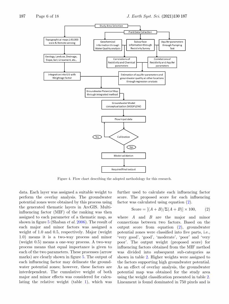
data. Each layer was assigned a suitable weight toperform the overlay analysis. The groundwaterpotential zones were obtained by this process usingthe generated thematic layers in ArcGIS. Multi-inCuencing factor (MIF) of the ranking was thenassigned to each parameter of a thematic map, asshown in Bgure 5 (Shaban et al. 2006). The result ofeach major and minor factors was assigned aweight of 1.0 and 0.5, respectively. Major (weight1.0) means it is a two-way process and minor(weight 0.5) means a one-way process. A two-wayprocess means that equal importance is given toeach of the two parameters. These processes (arrowmarks) are clearly shown in Bgure 5. The output ofeach inCuencing factor may delineate the ground-water potential zones; however, these factors areinterdependent. The cumulative weight of bothmajor and minor eAects was considered for calcu-lating the relative weight (table 1), which was

further used to calculate each inCuencing factorscore. The proposed score for each inCuencingfactor was calculated using equation (2).

Score ¼ Aþ Bð Þ=R Aþ Bð Þ½ � � 100; ð2Þ

where A and B are the major and minorconnections between two factors. Based on theoutput score from equation (2), groundwaterpotential zones were classiBed into Bve parts, i.e.,‘very good’, ‘good’, ‘moderate’, ‘poor’ and ‘verypoor’. The output weight (proposed score) forinCuencing factors obtained from the MIF methodwas divided into subsequent sub-categories asshown in table 2. Higher weights were assigned tothe factors supporting high groundwater potential.As an eAect of overlay analysis, the groundwaterpotential map was obtained for the study areausing the weight classiBcation presented in table 2.Lineament is found dominated in 750 pixels and is

Figure 4. Flow chart describing the adopted methodology for this research.


considered for high values and the remaining regionis given with low values. In the land-use map, tanksare given higher values followed by agriculturalland, and wasteland and built-up area for thelowest values. Considering the drainage density ofthe water bodies, the river is given higher valuesfollowed by the water bodies, the canal and theland area for the least values. The Bnalgroundwater potential map is validated with thespeciBc capacity obtained from the pumping test.

3.4 Groundwater Cow modelling

Most of the groundwater models are deterministic innature and are based on the conservation of mass,momentum, and energy. Deterministic groundwater

models like MODFLOW works on the principle ofDarcy’s law combined with the continuity equation.The three-dimensional movement of nearly incom-pressible groundwater through the porous medium isdescribed by the partial differential equation as shownin equation (3) (McDonald and Harbaugh 1988).

o

oxKxx

oh

ox

� �þ o

oyKyy

oh

oy

� �þ o

ozKzz

oh

oz

� �þW

¼ Ssoh

ot; ð3Þ

where Kxx, Kyy, and Kzz represent the values of thehydraulic conductivity in the x, y, and z directions,respectively; h is the water table head; W is avolumetric Cux per unit volume. W\0.0 indicates

Figure 5. Representation of interrelationship between the multi-inCuencing factors.

Table 1. Calculation of weightages for inCuencing factors.

Factor Major eAect Minor eAect

Proposed relative

weightage A + B

Proposed score for

each inCuencing factor

Lineament density 1+1 – 2 06

Drainage density 1+1 0.5 2.5 08

Landuse 1+1 0.5+0.5+0.5 3.5 10

Geo lithology 1+1+1+1 – 4 12

Geo soil 1 0.5 1.5 05

Depth to groundwater level 1+1+1+1+1+1+1 – 7 21

Computed aquifer parameters 1+1+1+1+1+1 – 6 18

Computed water quality 1+1+1+1+1 – 5 15

Slope 1 0.5 1.5 05

R = 33 R = 100


that Cow is going out of the groundwater system,and W[ 0.0 indicates that the Cow is going intothe system; Ss represents the speciBc storage of theporous material, and t denotes the time. Equa-tion (3) describes the groundwater Cow in aheterogeneous and anisotropic medium underunsteady conditions.Visual MODFLOW version 4.6 uses an inte-

grated Bnite-difference approximation and itera-tive approach to simulate groundwater Cow. Thesimulated model domain of the study area wasprepared in two layers with a grid framework of160 9 160 cells. The size of a cell was 170 9 157 m2,with the total active cells equal to 12,177. The

region outside the study area was assigned with aninactive Cow. The groundwater potential map wasdivided into 13 zones and each zone was consideredas boundaries for MODFLOW. The limitations ofboundaries were derived from the groundwaterpotential map and the thickness of each boundarywas derived from the electrical resistivity method.Figure 6 speciBes the 3D model layer with mean sealevel of ground elevation (colour code differentranges of elevation). The aquifer permeabilitybased on the pumping test varied from 0.008 to 12m/d as shown in table 3. High permeability valueprevailed in the alluvium region, which was mainlylocated under the highly weathered rock formation.

Table 2. Weightage classiBcation.

Factor Domain of eAect Weightage

Lineament density NW–SE (502 cells) 6

SW–NE (244 cells) 4

No lineaments (32191 cells) 2

Land use Water bodies 10

Agriculture 7

Waste lands 4

Built up 1

Geo lithology Charnockite 2

Weathered charnockite 4

Shale 6

Unconsolidated sediment 8

Unconsolidated lose sediment 10

Sand aquifer 12

Drain density River 8

Tanks/lake/pond 6

Canal 4

Drainage channel 2

Slope 0–0.2 5

0.2–0.4 3.5

0.4–0.8 2

0.8–2.3 0.5

Depth of groundwater \5 21

5–10 15

10–15 9

[15 3

Geo soil Clay 0.5

Silt clay 2

Sandy 3.5

Alluvium 5

Computed water quality \200 15

200–400 11

400–600 7

[600 3

Computed aquifer parameters \200 3

200–400 8

400–800 13

[800 18


November 2012 water level data was used as theinitial head value. In the model boundary condi-tion, the pumping rate was given a negative valuedue to the extraction of groundwater from thestudy region. The speciBc yield and speciBc storagevalues were chosen on the basis of geological for-mation. The model was run with the steady-stateconditions initially and later changed to transientstate conditions. The speciBc yield/storage coefB-cient is dependent on the area and rainfall. In thismodel, we considered constant value for both ofthese conditions. The control factor of this modelwas changed with all parameters except theobserved head. In groundwater modelling, 10% ofthe total rainfall quantity was taken as rechargequantity to the groundwater. Also, visual PEST(parameter estimation) and EVT (evapotranspi-ration) software packages were used for this study.The general purpose of a parameter estimationsoftware tool PEST (Doherty 2004) was to esti-mate the model parameters required to calibratethe solute transport model properly. PESTincludes the Gauss–Marquardt–Levenbergmethod which potentially suggests the advantagesrelative to manual calibration, especially for a

multi-dimensional and multi-species reactivesolute transport model.

3.5 Groundwater model calibrationand validation

The observed groundwater head (hobs) and simu-lated head (hsim) at the observation point ‘i’ are thetwo major parameters in the calibration and vali-dation process of a groundwater model. The rootmean square error (RMSE) of the residual wascalculated using equation (4) and the standarderror of the estimation (SEE) was calculated usingequation (5).

RMSE ¼ 1

n

Xni¼1

hsim � hobsð Þ2" #1=2

ð4Þ

SEE ¼1

n�1

Pni¼1 Ri � R

� �n

" #1=2ð5Þ

R ¼ 1

n

Xni¼1

hsim � hobsð Þ; ð6Þ

Figure 6. Three-dimensional view of the MODFLOW model for Walajabad Block.


where Ri is the difference between hsim and hobs at a

given point. R is a measure of the average residualvalue, as calculated in equation (6).In this study, calibration and validation were

performed using the Visual MODFLOW model.November 2012 to October 2013 was used as thecalibration period, and November 2013 to May2015 was used as the validation period. We usecorrelation coefBcient (R2), RMSE, and SEE as thestatistical parameters. Uncertainty in groundwatermodelling is inevitable for a number of reasons suchas elevation, permeability, speciBc yield, etc.Therefore, the conBdence intervals at a 0.05 sig-nificance level were considered in the analysis.In order to calculate the groundwater potential

zone (as shown in Bgure 7b), an unconBned aquiferwas divided into 13 zones. The groundwaterpotential zone was classiBed using an unconBnedaquifer proBle from the subsurface geology map.The output map of the multi-inCuential factor(section 3.3), i.e., groundwater potential zoneswere classiBed into 5 classes, i.e., ‘very good’,‘good’, ‘moderate’, ‘poor’ and ‘very poor’. Fur-thermore, the ‘very good’ class was divided intofour sub-classes, namely ‘hard rock’, ‘north allu-vium’, ‘south alluvium’, and ‘sedimentary’, and the‘good’ class was divided into three sub-classesnamely ‘hard rock’, ‘alluvium’, and ‘sedimentaryformations’. The classes ‘moderate’ to ‘very poor’was divided into two sub-classes, namely ‘hardrock’ and ‘sedimentary formations’.To analyse the groundwater trends in and

around the observation wells, the groundwater

estimation methodology (GREM 1997) was used,in which observation wells act as an indicator forthe periodical changes in groundwater level mea-surement. Dynamic groundwater potential and theamount of recharge/discharge of the study areawas assessed using the monthly groundwater levelCuctuation. Finally, the water balance was esti-mated as the difference between the volume ofwater leaving and entering the area. For the spec-iBed sub-regions, zone budgets can be computedusing the cell-by-cell Cow option with the transientsimulation. The zone budget does not determinethe cumulative budget; instead, it only providesoutput for a particular day.

4. Results and discussion

4.1 Evaluation of multi-inCuencing factors

To apply the multi-inCuencing factors (as dis-cussed in section 3.3), we divided layer-1 into fourzones based on soil classiBcation and layer-2 into13 zones based on the subsurface geology (seeBgure 7a and b, respectively). The classiBed rangesof the computed parameters are shown in table 2.These results are used in developing groundwaterpotential maps, in which transmissivity was usedas a water quantity parameter, and TDS is used asa water quality parameter. The spatial distributionmap of transmissivity and TDS (Bgure 3a and b)indicates that most of the study area falls in theleast transmissivity and moderate TDS zone. Thehigh transmissivity occurred in the region with

Table 3. Sensitivity values of aquifer parameters obtained from the groundwater Cow model.

Zone Type of formation

Kx/Ky [m/d]Kz

[m/d] Ss Sy

Effective

porosity

Total

porosity

Observed pumping

test (K [m/d])Initial Max Min

1 Hard rock very poor 0.6 1.1 0.1 0.06 0.00011 0.02 0.015 0.03 1.1

2 Sedimentary very poor 0.008 0.013 0.003 0.0008 0.000011 0.002 0.0015 0.003 0.05

3 Hard rock poor 3 8 0.5 0.3 0.0002 0.04 0.018 0.032 2.1

4 Sedimentary poor 0.07 0.12 0.02 0.007 0.00002 0.004 0.0018 0.0032 0.4

5 Hard rock moderate 4 9 0.8 0.4 0.0003 0.06 0.021 0.042 4.2

6 Sedimentary moderate 5 10 0.9 0.5 0.00003 0.006 0.0021 0.0042 –

7 Sedimentary good 6 11 1 0.6 0.0004 0.08 0.025 0.05 –

8 North alluvium good 7 12 2 0.7 0.0005 0.1 0.028 0.056 –

9 Hard rock good 8 13 3 0.8 0.0006 0.21 0.03 0.06 –

10 Sedimentary very good 9 14 4 0.9 0.0007 0.25 0.04 0.08 –

11 Hard rock very good 10 15 5 1 0.0008 0.28 0.051 0.102 –

12 North alluvium very good 11 16 6 1.1 0.0009 0.31 0.058 0.116 –

13 West hard rock very good 12 17 7 1.2 0.0012 0.35 0.064 0.128 –


alluvium formation. Figure 8(a) presents thegroundwater potential map for the WalajabadBlock determined by the overlay analysis using thesoil classiBcation and geology maps, as discussed in

section 3.3. The statistics, shown in Bgure 8(b)revealed that about 77% of the study area has‘moderate’ to ‘very good’ groundwater potential.The rest of the study area was classiBed as ‘poor’ to

Figure 7. (a) Layer-1 divided into 4 zones based on the soil classiBcation; (b) Layer-2 divided into 13 zones based on thesubsurface geology classiBcation with groundwater potential zone.

Figure 8. (a) Groundwater potential zonation map by integration of various parameters (geophysical, computed geochemical,computed aquifer parameters, groundwater level, landuse, slope, soil, and lineament) through weighted overlay technique.(b) Statistical output of groundwater potential area.


‘very poor’ groundwater potential zone due to clayformation in the northwest part and granitic andcharnockite rock formation in the southeast part ofthe study area (see Bgure 8a).

4.2 Calibration and validation resultsof the groundwater Cow model

The MODFLOW model was set up for the studyarea (see section 3.4). The groundwater Cow modelwas calibrated for 360 days and validated for therest of the period up to 840 days. The matchbetween model generated and observed head valuesare shown in Bgure 9(a–c) for the period of 360,720, and 840 days, respectively. The MODFLOWoutput shows a strong correlation (R2 = 0.982,0.979, and 0.97 on day number 360, 720, and 840,respectively) between the calibrated/validated andobserved groundwater heads.Table 4 shows the quantitative summary of

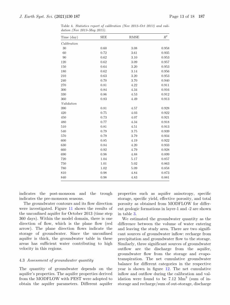
results obtained from the groundwater Cow model

during the calibration and validation periods. Theminimum and maximum SEE of all heads rangebetween 0.60 and 0.84 m for the calibration and0.73–1.04 m for the validation period. The RMSEof the observation wells ranges from 3.08 to 4.53 mand 4.03 to 5.17 m for calibration and validation,respectively. The R2 varies between 0.857 and0.958 in the model run period.Furthermore, the deviation between the

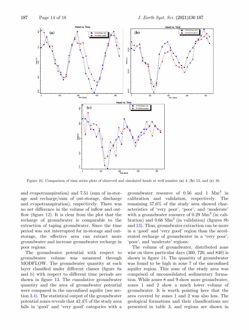
observed and calibrated/validated water level forthe whole calibration and validation period isshown as a time series for three selected wells (#4,#13, and #16) in Bgure 10(a–c), respectively. Agood match between the observed and simulatedwater levels was observed for all the three wells.These wells are selected as representative of thethree separate geological formations: #4 is instal-led in hard rock, #13 in sedimentary rocks, and#16 in alluvium formation. The water level Cuc-tuation in a particular well was due to seasonalrecharge and discharge. The crest of the diagram

Figure 9. Comparison of calculated and observed head during the calibration period at the time step (a) 360 days, (b) 720 days,and (c) 840 days.


indicates the post-monsoon and the troughindicates the pre-monsoon seasons.The groundwater contours and its Cow direction

were investigated. Figure 11 shows the results ofthe unconBned aquifer for October 2013 (time step360 days). Within the model domain, there is onedirection of Cow, which is the plane Cow (redarrow). The plane direction Cows indicate thestorage of groundwater. Since the unconBnedaquifer is thick, the groundwater table in theseareas has sufBcient water contributing to highvelocity in this regions.

4.3 Assessment of groundwater quantity

The quantity of groundwater depends on theaquifer’s properties. The aquifer properties derivedfrom the MODFLOW with PEST were adopted toobtain the aquifer parameters. Different aquifer

properties such as aquifer anisotropy, speciBcstorage, speciBc yield, eAective porosity, and totalporosity as obtained from MODFLOW for differ-ent geologic formations in layer-1 and -2 are shownin table 3.We estimated the groundwater quantity as the

difference between the volume of water enteringand leaving the study area. There are two signifi-cant sources of groundwater inCow: recharge fromprecipitation and groundwater Cow to the storage.Similarly, three significant sources of groundwateroutCow are the discharge from the aquifer,groundwater Cow from the storage and evapo-transpiration. The net cumulative groundwaterbalance for different categories in the respectiveyear is shown in Bgure 12. The net cumulativeinCow and outCow during the calibration and val-idation were found to be 7.12 Mm3 (sum of in-storage and recharge/sum of out-storage, discharge

Table 4. Statistics report of calibration (Nov 2012–Oct 2013) and vali-dation (Nov 2013–May 2015).

Time (day) SEE RMSE R2

Calibration

30 0.60 3.08 0.958

60 0.72 3.61 0.935

90 0.62 3.10 0.953

120 0.62 3.09 0.957

150 0.64 3.20 0.953

180 0.62 3.14 0.956

210 0.63 3.20 0.953

240 0.70 3.70 0.940

270 0.81 4.22 0.911

300 0.84 4.34 0.916

330 0.86 4.53 0.912

360 0.83 4.49 0.913

Validation

390 0.81 4.57 0.928

420 0.75 4.03 0.922

450 0.73 4.07 0.921

480 0.77 4.34 0.918

510 0.81 4.51 0.913

540 0.79 3.75 0.939

570 0.79 3.79 0.934

600 0.85 4.19 0.922

630 0.84 4.20 0.933

660 0.92 4.79 0.928

690 0.98 4.88 0.899

720 1.04 5.17 0.857

750 1.01 5.02 0.863

780 1.02 5.09 0.858

810 0.98 4.84 0.873

840 0.98 4.83 0.881


and evapotranspiration) and 7.51 (sum of in-stor-age and recharge/sum of out-storage, dischargeand evapotranspiration), respectively. There wasno net difference in the volume of inCow and out-Cow (Bgure 12). It is clear from the plot that therecharge of groundwater is comparable to theextraction of taping groundwater. Since the timeperiod was not interrupted for in-storage and out-storage, the eAective area can extract moregroundwater and increase groundwater recharge inpoor regions.The groundwater potential with respect to

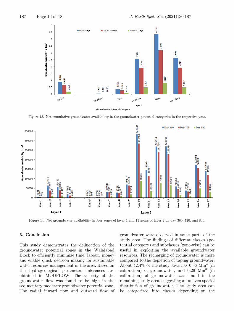
groundwater volume was measured throughMODFLOW. The groundwater quantity at eachlayer classiBed under different classes (Bgure 8aand b) with respect to different time periods areshown in Bgure 13. The cumulative groundwaterquantity and the area of groundwater potentialwere compared in the unconBned aquifer (see sec-tion 3.4). The statistical output of the groundwaterpotential zones reveals that 42.4% of the study areafalls in ‘good’ and ‘very good’ categories with a

groundwater resource of 0.56 and 1 Mm3 incalibration and validation, respectively. Theremaining 57.6% of the study area showed char-acteristics of ‘very poor’, ‘poor’, and ‘moderate’with a groundwater resource of 0.29 Mm3 (in cali-bration) and 0.66 Mm3 (in validation) (Bgures 8band 13). Thus, groundwater extraction can be morein a ‘good’ and ‘very good’ region than the accel-erated recharge of groundwater in a ‘very poor’,‘poor’, and ‘moderate’ regions.The volume of groundwater, distributed zone

wise on three particular days (360, 720, and 840) isshown in Bgure 14. The quantity of groundwaterwas found to be high in zone 7 of the unconBnedaquifer region. This zone of the study area wascomprised of unconsolidated sedimentary forma-tion. While zones 8 and 9 show more groundwater,zones 1 and 2 show a much lower volume ofgroundwater. It is worth pointing here that thearea covered by zones 1 and 2 was also less. Thegeological formations and their classiBcations arepresented in table 3, and regions are shown in

Figure 10. Comparison of time series plots of observed and simulated heads at well number (a) 4, (b) 13, and (c) 16.


Bgure 7(b). Such information will help in deter-mining the area where the recharge/dischargeof groundwater activity can take place in theregion. Quantifying the groundwater volume under

different zones and formations will be helpful ingroundwater management practices to improvethe use of groundwater resources in the studyarea.

Figure 11. Groundwater potential with velocity directions.

Figure 12. Net cumulative groundwater balance with different category in different time duration.


5. Conclusion

This study demonstrates the delineation of thegroundwater potential zones in the WalajabadBlock to eDciently minimize time, labour, moneyand enable quick decision making for sustainablewater resources management in the area. Based onthe hydrogeological parameter, inferences areobtained in MODFLOW. The velocity of thegroundwater Cow was found to be high in thesedimentary moderate groundwater potential zone.The radial inward Cow and outward Cow of

groundwater were observed in some parts of thestudy area. The Bndings of different classes (po-tential category) and subclasses (zone-wise) can beuseful in exploiting the available groundwaterresources. The recharging of groundwater is morecompared to the depletion of taping groundwater.About 42.4% of the study area has 0.56 Mm3 (incalibration) of groundwater, and 0.29 Mm3 (incalibration) of groundwater was found in theremaining study area, suggesting an uneven spatialdistribution of groundwater. The study area canbe categorized into classes depending on the

Figure 13. Net cumulative groundwater availability in the groundwater potential categories in the respective year.

Figure 14. Net groundwater availability in four zones of layer 1 and 13 zones of layer 2 on day 360, 720, and 840.


concentration of the produced groundwater andrecharged groundwater. The production ofgroundwater can be concentrated more in a ‘good’and ‘very good’ area than the rapid recharging ofgroundwater, concentrated in a ‘very poor’, ‘poor’,and ‘moderate’ area. The Bndings from this studycan be used to develop natural recharge practicesin the low potential region. The sensitivity valuesof aquifer parameters derived from the model canact as standard aquifer parameters for futurestudies in the Walajabad region. The approachused in this study is an empirical method for theexploration of groundwater potential zones, whichsuccessfully delineated groundwater potentialzones in the Walajabad Block.

Acknowledgements

This paper was supported by a postdoctoralresearch fellowship under the initiation grant fromthe Indian Institute of Science Education andResearch Bhopal (INST/EES/2017067). The dataused in this study were collected during the Ph.D.of the Brst author at Anna University, Chennai.The authors thank Dr Suresh A Kartha at theIndian Institute of Technology Guwahati, for hiscomments on the earlier version of the manuscript.We also thank two anonymous reviewers for theirvaluable comments.

Author statement

Dr Mathiazhagan collected the data. Dr SanjeevJha supervised Dr Mathiazhagan in performing theanalysis and writing the manuscript. Dr AshisBiswas helped in editing the manuscript.

References

Ahmed S, de Marsily G and Talbot A 1988 Combined use ofhydraulic and electrical properties of an aquifer in a geosta-tistical estimation of transmissivity; Groundwater 26(1)78–86, https://doi.org/10.1111/j.1745-6584.1988.tb00370.x.

Bahir M, Ouazar D and Ouhamdouch S 2019 Hydrogeochem-ical investigation and groundwater quality in Essaouiraregion, Morocco; Mar. Freshw. Res. 70(9) 1317, https://doi.org/10.1071/mf18319.

Bauer S, Bayer-Raich M, Holder T, Kolesar C, M€uller D andPtak T 2004 QuantiBcation of groundwater contaminationin an urban area using integral pumping tests; J. Contam.Hydrol. 75(3–4) 183–213, https://doi.org/10.1016/j.jconhyd.2004.06.002.

Candela L, von Igel W, Elorza F J and Aronica G 2009 Impactassessment of combined climate and management scenarioson groundwater resources and associated wetland (Majorca,Spain); J. Hydrol. 376(3–4) 510–527, https://doi.org/10.1016/j.jhydrol.2009.07.057.

Cassiani G and Medina M A 1997 Incorporating auxiliarygeophysical data into groundwater Cow parameter estima-tion; Groundwater 35(1) 79–91.

Central Ground Water Board (CGWB) 2012 Aquifer Infor-mation System and Aquifer Management Plan, 396 Tier IItraining course, Chennai, http://cgwb.gov.in/RGI/Tier%20II%20Training%20Module%20English.pdf.

Dar I A, Sankar K and Dar M A 2010 Remote sensingtechnology and geographic information system modeling:An integrated approach towards the mapping of ground-water potential zones in Hardrock terrain, Mamundiyarbasin; J. Hydrol. 394(3–4) 285–295, https://doi.org/10.1016/j.jhydrol.2010.08.022.

Doherty J 2004 PEST, Model independent parameter estima-tion user manual, 5th edn, Watermark NumericalComputing.

Falke J A, Fausch K D, Magelky R, Aldred A, Durnford D S,Riley L K and Oad R 2011 The role of groundwaterpumping and drought in shaping ecological futures forstream Bshes in a dryland river basin of the western GreatPlains, USA; Ecohydrology 4(5) 682–697, https://doi.org/10.1002/eco.158.

Groundwater Resource Estimation Methodology (GREM)1997 Report of the groundwater resource estimation com-mittee; Ministry of Water Resources, Government of India,New Delhi.

Gupta A K, Tyagi P and Sehgal V K 2011 Drought disasterchallenges and mitigation in India: Strategic appraisal;Curr. Sci. 1795–1806.

Halder S, Roy M B and Roy P K 2020 Analysis of groundwaterlevel trend and groundwater drought using StandardGroundwater Level Index: A case study of an eastern riverbasin of West Bengal, India; SN Appl. Sci. 2(3) 1–24.

Jha S K, Mariethoz G, Matthews G, Vial J and Kelly B F J2015 InCuence of alluvial morphology on upscaled hydraulicconductivity; Groundwater 54(3) 384–393, https://doi.org/10.1111/gwat.12378.

Jha S K, Comunian A, Mariethoz G and Kelly B 2014Parameterization of training images for aquifer 3D faciesmodeling integrating geological interpretations and statis-tical inference; Water Resour. Res. 50(10) 7731–7749,https://doi.org/10.1002/2013WR014949.

Kumar M G, Bali R and Agarwal A 2009 Integration of remotesensing and electrical sounding data for hydrogeologicalexploration – A case study of Bakhar watershed, India/Int�egration de donn�ees de t�el�ed�etection et de sondages�electriques pour l’exploration hydrog�eologique – �etude decas du bassin versant de Bakhar, Inde; Hydrol. Sci. J. 54(5)949–960, https://doi.org/10.1623/hysj.54.5.949.

Li F, Feng P, Zhang W and Zhang T 2013 An integratedgroundwater management mode based on control indexes ofgroundwater quantity and level; Water Resour. Manag.27(9) 3273–3292, https://doi.org/10.1007/s11269-013-0346-8.

Liu Y, Yamanaka T, Zhou X, Tian F and Ma W 2014Combined use of tracer approach and numerical simulationto estimate groundwater recharge in an alluvial aquifer


system: A case study of Nasunogahara area, central Japan;J. Hydrol. 519 833–847, https://doi.org/10.1016/j.jhydrol.2014.08.017.

Mart�ınez-Santos P and Andreu J 2010 Lumped and dis-tributed approaches to model natural recharge in semi-aridkarst aquifers; J. Hydrol. 388(3–4) 389–398, https://doi.org/10.1016/j.jhydrol.2010.05.018.

Mastrocicco M, Vignoli G, Colombani N and Zeid N A 2010Surface electrical resistivity tomography and hydrogeolog-ical characterization to constrain groundwater Cow model-ing in an agricultural Beld site near Ferrara (Italy);Environ. Earth Sci. 61(2) 311–322, https://doi.org/10.1007/s12665-009-0344-6.

Mathiazhagan M, Selvakumar T and Madhavi G 2015 Surfacegeo-electrical sounding for the determination of aquifercharacteristics in part of the Palar sub-basin, Tamilnadu,India; JCHPS Special Issue 8 1–7.

McDonald M G and Harbaugh A W 1988 A modular three-dimensional Bnite-difference groundwater Cow model, USGeological Survey Reston, VA.

Mikita M, Yamanaka T and Lorphensri O 2011 Anthropogenicchanges in a conBned groundwater Cow system in theBangkok basin, Thailand. Part I: Was groundwater-recharge enhanced?; Hydrol. Process. 25(17) 2726–2733,https://doi.org/10.1002/hyp.8013.

Mukherjee S, Bebermeier W and Sch€utt B 2018 An overviewof the impacts of land use land cover changes (1980–2014)on urban water security of Kolkata; Land 7(3) 91, https://doi.org/10.3390/land7030091.

Oh H J, Kim Y S, Choi J K, Park E and Lee S 2011 GISmapping of regional probabilistic groundwater potential inthe area of Pohang City, Korea; J. Hydrol. 399(3–4)158–172, https://doi.org/10.1016/j.jhydrol.2010.12.027.

Palma H C and Bentley L R 2007 A regional-scale ground-water Cow model for the Leon–Chinandega aquifer,Nicaragua; Hydrogeol. J. 15(8) 1457–1472, https://link.springer.com/article/https://doi.org/10.1007/s10040-007-0197-6?referrer=Baker.

Panda D K, Mishra A, Jena S, James B and Kumar A 2007 TheinCuence of drought and anthropogenic eAects on groundwa-ter levels in Orissa, India; J. Hydrol. 343(3–4) 140–153.

Patra S, Sahoo S, Mishra P and Mahapatra S C 2018 Impactsof urbanization on land use/cover changes and its probable

implications on local climate and groundwater level; J.Urban Manag. 7(2) 70–84.

Pisinaras V, Petalas C, Tsihrintzis V and Karatzas G 2013Integrated modeling as a decision-aiding tool for ground-water management in a Mediterranean agricultural water-shed; Hydrol. Process. 27(14) 1973–1987, https://doi.org/10.1002/hyp.9331.

Sashikkumar M, Selvam S, Kalyanasundaram V L and JohnnyJ C 2017 GIS based groundwater modeling study to assessthe eAect of artiBcial recharge: A case study from Koda-ganar river basin, Dindigul district, Tamil Nadu; J. Geol.Soc. India 89(1) 57–64.

Sekhar M, Rasmi S, Sivapullaiah P and Ruiz L 2004Groundwater Cow modeling of Gundal sub-basin in Kabiniriver basin, India; Asian J. Water Environ. Pollut. 1(1, 2)65–77.

Shaban A, Khawlie M and Abdallah C 2006 Use of remotesensing and GIS to determine recharge potential zones: Thecase of Occidental Lebanon; Hydrogeol. J. 14(4) 433–443,https://doi.org/10.1007/s10040-005-0437-6.

Slater L 2007 Near surface electrical characterization ofhydraulic conductivity: From petrophysical propertiesto aquifer geometries – A review; Surv. Geophys.28(2–3) 169–197, https://doi.org/10.1007/s10712-007-9022-y.

Wang H, Gao J E, Zhang M J, Li X H, Zhang S L and Jia L Z2015 EAects of rainfall intensity on groundwater rechargebased on simulated rainfall experiments and a groundwaterCow model; Catena 127 80–91, https://doi.org/10.1016/j.catena.2014.12.014.

Zektser I S and Lorne E 2004 Groundwater Resources of theWorld and Their Use, Ihp Series on Groundwater,UNESCO, Paris.

Zhang H and Hiscock K 2010 Modelling the impact of forestcover on groundwater resources: A case study of theSherwood Sandstone aquifer in the East Midlands, UK;J. Hydrol. 392(3–4) 136–149, https://doi.org/10.1016/j.jhydrol.2010.08.002.

Zume J and Tarhule A 2008 Simulating the impacts ofgroundwater pumping on stream – aquifer dynamics insemi-arid northwestern Oklahoma, USA; Hydrogeol.J. 16(4) 797–810, https://doi.org/10.1007/s10040-007-0268-8.

Corresponding editor: RIDDHI SINGH


Assessment of groundwater mass balance and zone budget …

Documents

Transcript of Assessment of groundwater mass balance and zone budget …