Assessment of a multi-species in situ FTIR for precise atmospheric ...

Atmos. Meas. Tech., 6, 1153–1170, 2013www.atmos-meas-tech.net/6/1153/2013/doi:10.5194/amt-6-1153-2013© Author(s) 2013. CC Attribution 3.0 License.

EGU Journal Logos (RGB)

Advances in Geosciences

Open A

ccess

Natural Hazards and Earth System

Sciences

Open A

ccess

Annales Geophysicae

Open A

ccess

Nonlinear Processes in Geophysics

Open A

ccess

Atmospheric Chemistry

and Physics

Open A

ccess

Atmospheric Chemistry

and Physics

Open A

ccess

Discussions

Atmospheric Measurement

TechniquesO

pen Access

Atmospheric Measurement

Techniques

Open A

ccess

Discussions

Biogeosciences

Open A

ccess

Open A

ccess

BiogeosciencesDiscussions

Climate of the Past

Open A

ccess

Open A

ccess

Climate of the Past

Discussions

Earth System Dynamics

Open A

ccess

Open A

ccess

Earth System Dynamics

Discussions

GeoscientificInstrumentation

Methods andData Systems

Open A

ccess

GeoscientificInstrumentation

Methods andData Systems

Open A

ccess

Discussions

GeoscientificModel Development

Open A

ccess

Open A

ccess

GeoscientificModel Development

Discussions

Hydrology and Earth System

Sciences

Open A

ccess

Hydrology and Earth System

Sciences

Open A

ccess

Discussions

Ocean Science

Open A

ccess

Open A

ccess

Ocean ScienceDiscussions

Solid Earth

Open A

ccess

Open A

ccess

Solid EarthDiscussions

The Cryosphere

Open A

ccess

Open A

ccess

The CryosphereDiscussions

Natural Hazards and Earth System

Sciences

Open A

ccess

Discussions

Assessment of a multi-species in situ FTIR for preciseatmospheric greenhouse gas observations

S. Hammer1, D. W. T. Griffith 2, G. Konrad1, S. Vardag1, C. Caldow2, and I. Levin1

1Institut fur Umweltphysik, University of Heidelberg, Heidelberg, Germany2School of Chemistry, University of Wollongong, Wollongong, Australia

Correspondence to:S. Hammer ([email protected])

Received: 27 March 2012 – Published in Atmos. Meas. Tech. Discuss.: 22 May 2012Revised: 18 March 2013 – Accepted: 22 March 2013 – Published: 7 May 2013

Abstract. We thoroughly evaluate the performance of amulti-species, in situ Fourier transform infrared (FTIR) anal-yser with respect to high-accuracy needs for greenhousegas monitoring networks. The in situ FTIR analyser isshown to measure CO2, CO, CH4 and N2O mole frac-tions continuously, all with better reproducibility than theinter-laboratory compatibility (ILC) goals, requested by theWorld Meteorological Organization (WMO) for the GlobalAtmosphere Watch (GAW) programme. Simultaneously de-terminedδ13CO2 reaches reproducibility as good as 0.03 ‰.Second-order dependencies between the measured compo-nents and the thermodynamic properties of the sample, (tem-perature, pressure and flow rate) and the cross sensitivitiesamong the sample constituents are investigated and quanti-fied. We describe an improved sample delivery and controlsystem that minimises the pressure and flow rate variations,making post-processing corrections for those quantities non-essential. Temperature disequilibrium effects resulting fromthe evacuation of the sample cell are quantified and improvedby the usage of a faster temperature sensor. The instrumenthas proven to be linear for all measured components in theambient concentration range. The temporal stability of theinstrument is characterised on different time scales. Instru-ment drifts on a weekly time scale are only observed forCH4 (0.04 nmol mol−1 day−1) andδ13CO2 (0.02 ‰ day−1).Based on 10 months of continuously collected quality con-trol measures, the long-term reproducibility of the instru-ment is estimated to±0.016 µmol mol−1 CO2, ±0.03 ‰δ13CO2,±0.14 nmol mol−1 CH4,±0.1 nmol mol−1 CO and±0.04 nmol mol−1 N2O. We propose a calibration and qual-ity control scheme with weekly calibrations of the instru-ment that is sufficient to reach WMO-GAW inter-laboratorycompatibility goals.

1 Introduction

The globally distributed in situ greenhouse gas (GHG) mon-itoring network is one of the mainstays of modern climateresearch. Only a few continuous atmospheric CO2 recordsgo back to the 1950s (Keeling et al., 1976), but nowadaysmany stations monitor nearly all long-lived GHGs with insitu instrumentation (Worthy, 2003; Messager et al., 2008).The required accuracy and precision for measurements ofthe most important GHG species have been set to limitsthat allow extracting the required biogeochemical informa-tion from spatial differences that are needed for quanti-fying continental scale GHG fluxes and their inter-annualchanges (WMO report No. 5, 1981, cited in Francey andSteele, 2003). Over the most recent decades, non-dispersiveinfrared (NDIR) analysis of CO2 and gas chromatography(GC) of CO2 and all other long-lived GHGs has been provento provide this accuracy and precision; they have thus be-come standard techniques for GHG monitoring. Both tech-niques require special care, maintenance, frequent calibra-tion and quality control measures to guarantee data qual-ity; they are thus labour intensive in their day-to-day oper-ation. In recent years, optical techniques like Cavity Ring-Down Spectroscopy (CRDS), Off-Axis Integrated CavityOutput Spectroscopy (OA-ICOS) or Fourier transform in-frared spectroscopy (FTIR) have reached similar or evenbetter precisions than traditional GC systems. Contrary tothe discrete samples measured with GC systems, these tech-niques offer real continuous data acquisition and are in gen-eral less labour intensive (Winderlich et al., 2010). Opticaltechniques can be divided into two fundamentally differentmethods: (1) laser-based methods and (2) broadband infraredspectroscopy. The major distinctive feature between them isthe range of the recorded and evaluated absorption spectrum.

Published by Copernicus Publications on behalf of the European Geosciences Union.

1154 S. Hammer et al.: Precise atmospheric greenhouse gas observations

Whereas laser-based instruments are tuned to a narrow ab-sorption window with ideally little interference from otherspecies, the FTIR scans a broad IR range, thereby offeringthe possibility to measure a large number of species simul-taneously. The laser-based techniques like CRDS and OA-ICOS have been extensively and successfully studied by theGHG measurement community; some instruments have al-ready found their way into today’s observational networks(Winderlich et al., 2010).

Another benefit of optical spectroscopy is the possibilityof discriminating isotopologues, e.g. it allows for continu-ous measurement ofδ13CO2. The challenge of isotopologue-selective measurements is, however, to accurately determinethe absolute sums of all individual isotopologues. To do so,either all relevant isotopologues have to be measured inde-pendently, as done by the in situ FTIR analyser, or assump-tions on the mean relation between13CO2 and 12CO2 inclean air have to be taken into account during evaluationand/or should be already incorporated in the calibration ofthe instrument (Chen et al., 2010).

So far, studies discussing the use of the in situ FTIRtechnique for GHG monitoring purposes are rare, althoughpromising (Griffith et al., 2010). Therefore, detailed investi-gations of the potential and the possible shortcomings of thistechnique with respect to the accuracy goals set by WMO(World Meteorological Organization)/GAW (Global Atmo-sphere Watch) experts for clean background air monitoringshould be performed before it is used widely within the mon-itoring community. In particular, questions regarding long-term stability, calibration frequency and cross sensitivity ofdifferent trace gases have to be addressed. In the present pa-per we report on experiments that were performed at theUniversity of Heidelberg Institut fur Umweltphysik (IUP),on instrument repeatability, parameter- and cross sensitiv-ity, linearity and long-term stability of an in situ FTIR anal-yser that was designed and built at the University of Wol-longong, Australia (UoW) (Griffith et al., 2012). These datahave been gathered in the IUP laboratory as well as in thecourse of the ICOS (Integrated Carbon Observation Sys-tem, http://www.icos-infrastructure.eu/) Demonstration Ex-periment, where the instrument was run at two field stationsin Europe. The UoW FTIR instrument is subject to an on-going development process, and many findings of this pa-per have already led to improvements in newer instrumentversions. Nonetheless, our findings are generally applicableto any in situ FTIR instrument and can therefore be used asguideline for in situ FTIR users in order to raise awarenessfor high-end accuracy applications.

In the first part of this paper (Sect. 2), the initial in-strumental setup and its subsequent modifications are intro-duced, along with a description of the spectroscopic retrievaltechnique and the standard operating conditions used. Sec-tion 3 discusses and quantifies second-order sensitivities ofthe measured mole fractions to the thermodynamic proper-ties of the sample, such as temperature and pressure. The is-

44

1

2

3

Figure 1. Schematic set-up of the in situ FTIR analyser. The blue parts have been replaced 4

with the red parts in the final IUP set-up. The modifications include Mass Flow Controllers 5

(MFC) and Electronic Pressure Controllers (EPC) and replace the original needle valve - 6

Flow Meter (FM) unit. 7

8

Fig. 1. Schematic setup of the in situ FTIR analyser. The blue partshave been replaced with the red parts in the final IUP setup. Themodifications include mass flow controllers (MFC) and electronicpressure controllers (EPC) and replace the original needle valve–flow meter (FM) unit.

sue of inter-species cross sensitivities is discussed as well.This section is extended in Appendix A by an evaluation ofthe thermodynamic conditions in the cell after sample ex-change. After characterising the instrument’s sensitivities, itsresponse function in the ambient concentration range is in-vestigated in section 4, followed by an exhaustive study oninstrument stability and performance on short (weekly) andlong (monthly) time scales in Sect. 5. This section also in-cludes an empirical determination of the required calibrationfrequency. An overall error assessment is given in Sect. 6.The paper concludes with a discussion of the general appli-cability of the in situ FTIR analyser for background green-house gas monitoring purposes, as well as a recommendationfor further improvement of the instrument performance.

2 Instrumental setup and sample handling

Griffith et al. (2010, 2012) describe the improved in situFTIR instrument used in the present work, which is basedon the early version of the instrument as described by Esleret al. (2000a, b) and findings of the current study. The essen-tial parts of the in situ FTIR analyser and the modificationsintroduced in Heidelberg, based on the first year’s findings,are presented here. The different hardware configurations ofthe instrument throughout this study are specified in Sect. 2.1below.

2.1 Instrument components and sample handling

The instrument consists of a commercially available FTIR in-terferometer (IRcube, Bruker Optics, Germany) and a 3.5 Lmulti-pass cell with 24 m optical path length (PA-24, InfraredAnalysis, Anaheim, USA) (see Fig. 1). To avoid artefacts, the

Atmos. Meas. Tech., 6, 1153–1170, 2013 www.atmos-meas-tech.net/6/1153/2013/

http://www.icos-infrastructure.eu/

S. Hammer et al.: Precise atmospheric greenhouse gas observations 1155

transfer optics between the interferometer, the multi-pass celland the interferometer housing itself are permanently flushedwith high-purity nitrogen (99.999 %). The FTIR interferom-eter and the multi-pass cell are aligned via an optical benchsituated in an actively temperature controlled enclosure. Inits basic configuration the in situ FTIR analyser has fourseparate sample inlets and air is drawn through the instru-ment using an oil-free vacuum pump (model MV2NT, Vac-uubrand, Germany) at the outlet of the instrument. More in-take lines can be added via a multi-position valve (MWSD16selection valve, Valco, USA) connected to any of the fourstandard inlets.

The in situ FTIR analyser has a built-in sample-drying sys-tem consisting of a 24 inch (0.6 m) Nafion® dryer (Perma-pure, Toms River, NJ, USA) operated in counter-flow mode,followed by a chemical dryer filled with magnesium perchlo-rate (Mg(ClO4)2) for uptake of residual water. The Nafiondryer is placed in a separate compartment of the instrument,along with tubing, valves, PC and power supplies. The dry-ing system reaches a dew point of≈−65◦C and can be by-passed if measurement of H2O isotopologues is of interest.The dew point is estimated based on the uncalibrated H2Omeasurements of the in situ FTIR analyser. For more de-tails on H2O isotopologue measurements, refer to Parkes etal. (2013).

The modifications of the instrumental setup performed inHeidelberg are all related to sample handling as well as con-trolling and measuring sample conditions. In the followingthe different instrumental setups are introduced:

1. Initial UoW setup: the sample flow through the systemis adjusted with a needle valve (NV) and monitored us-ing a flow meter (FM) mounted at the outlet of the cell(see Fig. 1, blue parts). The multi-pass cell is equippedwith an in situ PT100 resistance temperature detector(RTD) and with a pressure sensor (HPM-760s, TeledyneHastings, USA) to determine the thermodynamic sam-ple properties. Both sensors are assumed to be linearand calibrated using a simple two point calibration.

2. ICOS Demonstration Experiment setup: for additionalstabilisation of the sample flow and pressure in thecell, the ICOS Demonstration Experiment setup usedan external add-on mass flow controller (MFC) (2 slpm,MKS Instruments, USA) in between the outlet of themulti-port valve and the instrument air inlet (see Fig. 1).Pressure and temperature sensors remain unchanged.

3. Intermediate setup: the intermediate setup has one built-in mass flow-controller (Model 3660, Kofloc, Japan), re-placing the needle-valve flow meter unit as well as theexternal MKS flow controller (compare Fig. 1). The in-ternal MFC is located at the outlet of the cell and canbe operated in flow control mode or in pressure controlmode when combined with a software embedded feed-back loop to the pressure sensor. The RTD temperature

sensor in the cell was also replaced by a faster respond-ing J-type thermocouple. The thermocouple was cen-tred in the cell to get a more representative temperaturemeasurement. The temperature sensor of the enclosuretemperature control was removed from the cell wall.This version was equivalent to that originally providedby Ecotech (Spectronus GHG analyser, Knoxfield, Aus-tralia) in the first commercially available versions of theanalyser.

4. IUP setup: in addition to the intermediate setup, thesample pressure in the cell is controlled by an elec-tronic pressure controller (EPC) (P-602CV EL-Press,Bronkhorst, The Netherlands) mounted at the cell inlet(see, Fig. 1). This configuration is functionally equiv-alent to the current version described by Griffith etal. (2012), with both pressure and flow control andavailable commercially from Ecotech.

In all configurations the cell is operated at slight overpres-sure to increase signal-to-noise ratio and to ease leak detec-tion. A diaphragm pump fitted with an EPDM membrane (N86 KN.18, KNF Neuberger, Germany) is used to pressuriseambient air up to 1800 hPa. Long-term GC experience hasshown that these pumps have negligible effects on the mea-sured species. Nevertheless, each pump is tested for contam-ination prior to its use by sucking air from a free-flowingcylinder and directing it to the GC. The free flowing cylin-der air is alternately analysed by the GC with and withoutthe pump to account for the fast drainage effects of cylindersand regulators (Hammer et al., 2012).

2.2 Spectroscopic concentration retrieval

The spectral range of the IRcube is 1800–7500 cm−1 witha 1 cm−1 resolution. The in situ FTIR analyser recordsand stores a broadband absorption spectrum from 1800–5000 cm−1 for each measurement. The recorded spectra areanalysed online by non-linear least squares fitting of sectionsof the measured spectrum with a modelled spectrum calcu-lated from the HITRAN database of absorption line parame-ters (Rothman et al., 2005). The theoretical spectrum is cal-culated by MALT (multiple atmospheric layer transmission)as described elsewhere (Griffith, 1996; Griffith et al., 2003,2012). Three separate spectral regions are fitted for eachspectrum: 2150–2320 cm−1 for 13CO2, 12CO2, CO and N2O,3001–3150 cm−1 for CH4 and 3520–3775 cm−1 for CO2 (allisotopologues) and residual H2O. The spectral analysis de-termines the molar concentrations (ci [mol m−3]) of each gasspecies. To convert molar concentrations into mole fractions(xi [mol mol−1]), sample pressure and temperature need tobe taken into account:

xi(wet) = ci/(p/RT), (1)

wherep is the absolute cell pressure,T the absolute tem-perature,R the universal gas constant andi the investigated

www.atmos-meas-tech.net/6/1153/2013/ Atmos. Meas. Tech., 6, 1153–1170, 2013


species. Since residual water is determined from the spec-trum for each sample, dry-air mole fractionsxi can easily bederived from

xi(dry) = xi(wet)/(1− xH2O). (2)

2.3 Standard operating conditions (SOC)

The standard operating conditions (SOC) of the in situ FTIRcomprises the instrument settings, measurement mode andinterval as well as sample change-over strategies.

– Instrument settings: the enclosure temperature is set to30.0◦C. It is stable within±0.06◦C, which leads to astability of the cell temperature of±0.02◦C for mod-erately stable laboratory conditions of±1◦C. All sam-ples are dried using the built-in drying system (Fig. 1).The sample flow rate is set to 1±0.02 slpm. For theICOS Demonstration Experiment setup, the cell pres-sure was set via sample delivery pressure and was keptat 1100±8 hPa. In the modified IUP setup, sample pres-sure and flow are controlled separately to better than±0.1 hPa and±0.008 slpm, respectively.

– Measurement mode: the in situ FTIR analyser offersstatic and dynamic measurement modes. In the staticmeasurement mode, the cell is filled with the sample,sample flow is shut off and the sample is subsequentlymeasured for a certain measurement interval. The dy-namic mode measures the sample for a certain inter-val while it is continuously flushed through the cell.Since systematic differences between the two measure-ment modes were found (see. Sect. 3.5), we chose toflush both sample types, ambient air and air from high-pressure cylinders, continuously through the cell withthe same flow rate of 1.00±0.02 slpm. This approachis taken to assure comparability for both sample types.

– Measurement interval: the measurement interval is setto 3 min, in which a 2.5 min spectra collection period isfollowed by 0.5 min online analysis with the installedPC. This time interval was chosen as a compromisebetween instrument precision (increasing with averag-ing time; see Sect. 5.1) and smoothing out natural vari-ability in the ambient air, which itself blurs the aver-aged spectra. For example, in Heidelberg CO values canchange by more than 100 nmol mol−1 within 30 minduring rush-hour situations (Hammer et al., 2009). Inaddition, the 3 min measurement interval equals the ap-proximate turn over time of the sample in the cell at1 slpm flow rate.

– Sample change-over strategy: under SOC each sam-ple change-over, i.e. changing from ambient to cylin-der measurements and vice versa, involves a two-stepevacuation of the cell that is described in detail in Ap-pendix A. Possible disadvantages of evacuating the cell,

i.e. by disturbance of moisture or temperature equilib-rium, will be discussed in Sect. 3.6 and Appendix A.In SOC each cylinder measurement is performed over30 min, including the sample change-over, and requiresa total gas volume of about 27 L of air.

3 Residual sensitivities to sample properties and inter-species cross sensitivities

3.1 Origin of residual and cross sensitivities

3.1.1 Residual sensitivities to sample properties

The line shapes of the investigated species are dependenton pressure- and Doppler broadening and thus depend onsample properties like pressure and temperature. For bothbroadening effects, temperature- and pressure-dependent linewidths are tabulated in the HITRAN 2004 database (Roth-man et al., 2005); they are considered by the FTIR spectraevaluation program MALT (Griffith, 1996), using the mea-sured sample temperature and pressure. However, the lineshape parameters themselves are subject to ongoing improve-ment: as an example, for the CO2 line parameters, differencesof up to a few percent are reported in recent studies (Long etal., 2011; Nakamichi et al., 2006). Small errors in the HI-TRAN parameters lead to systematic biases in the retrievedmolar concentrations. We will refer to this error contributionas theline shape error.

Furthermore, the retrieved molar concentrations are biasedby potential offsets in the measured sample temperature andpressure since these quantities are directly used in MALT toselect the tabulated line shape parameters. In the following,these introduced retrieval biases are referred to as theintro-duced spectroscopic error.

In addition to the line shape and the introduced spectro-scopic error, the conversion from molar concentrations tomole fractions (see Eq. 1) constitutes another direct link tothe measured sample properties and their precision. This di-rect link is established through the sample density (dependenton temperature and pressure) and is thus approximately thesame for all species on a percentage basis. This emphasisesthe importance of accurate sample temperature- and pressuremeasurements to minimise thedensity error. Accurate andtemporally stable sensor calibration down to a level of 0.01 %is thus important to reach the required accuracy and precisionfor the greenhouse gas measurements. Determining the aver-age sample temperature is challenging since temperature isnot homogeneous within the cell. In all current setups tem-perature is measured in one location only, assuming a con-stant temperature distribution. However, thetrue temperaturedistribution in the cell depends on sample flow rate and in-jection (see Appendix A). The measured mole fractions maythus implicitly depend on the flow rate as well.



The combination of the line shape, the introduced spec-troscopic and the density error are thus the underlying causeof residualpressure and temperature sensitivities. The termresidualis used as the first-order changes of these parametersare already accounted for and only the deviations between themeasured and thetrue sample and spectroscopic propertiescause these effects. Since all error contributions are coupled,it is experimentally not possible to disentangle the error con-tributions. However, in a synthetic MALT study it is possibleto investigate the introduced spectroscopic and the densityerror. This approach will be discussed in Sects. 3.3 and 3.4.

3.1.2 Inter-species cross sensitivities

Apart from residual pressure, temperature and flow sensitiv-ities, additional inter-species cross sensitivities exist, whichare caused by overlapping spectral absorption regions of dif-ferent trace species. Generally, the MALT least-squares fit isable to disentangle the contributions to absorption at eachwave number and to attribute their shares to the differentspecies. Nevertheless, the MALT algorithm, the measuredspectra and the HITRAN data are not perfect, and small inter-species cross sensitivities remain. Since H2O absorption inthe infrared region occurs at many different wavelengths, theinter-species sensitivity to residual water vapour is notice-able for all investigated species, apart from CH4. The second-strongest absorber in ambient air is CO2. Since the13CO2,and N2O absorptions in the 2150–2320 cm−1 region overlapwith strong absorption of12CO2, measurable inter-speciescross sensitivities to CO2 also exist.

3.2 Sensitivity experiments

We carried out a series of dedicated experiments to detectand quantify the residual sensitivities to sample properties(pressure, temperature and flow) and the cross sensitivities(H2O and CO2) of the in situ FTIR analyser. If applicable,these measurements were used to define correction functionsfor each species. In all experiments the investigated sam-ple property or species was systematically varied, while allother parameters or species were kept as constant as possible.The experiments have been repeated several times over thecourse of 1 yr to investigate temporal stability of the sensitiv-ities. For each test we used ambient Heidelberg air collectedin high-pressure cylinders with a diving compressor (modelP3W, Bauer, Germany) and dried to a dew point of approxi-mately−40◦C. The cylinders (40L L6X aluminium, Luxfer,UK) and pressure regulators (model 14A, Scott SpecialtyGases, USA) have proven to be suitable for high-precisionGHG measurements by GC analysis (Hammer, 2008). TheGHG concentrations in each test cylinder were checked fordrifts by GC analysis before and after use.

To investigate the residual sensitivities against tempera-ture, pressure and flow, the respective parameter was tuned atthe FTIR analyser itself. Determining the inter-species cross

sensitivities involved a custom-made mixing device, consist-ing of two mass flow controllers (MFC) and a scrubbingagent, either Ascarite® for CO2, or Mg(ClO4)2 for H2O. Themixing device divides the sample stream into two branches,one of them containing the scrubbing agent. The flow con-trollers are used to provide varying flow ratios in the twobranches. After scrubbing, both branches are re-combinedand the mixed gas is injected into the in situ FTIR analyser.

A residual- or cross-sensitivity experiment determines theconcentrations of a fixed sample with respect to at least fourdifferent settings of the investigated sensitivity parameter.For each setting we allowed sufficient time to re-establishequilibrium in the whole system, i.e. until the variability inCO2 was on the order of the instrument’s repeatability, andthen held constant for at least 30 min. The averaged dry-airmole fractions for each equilibrium setting were then used toquantify the sensitivity. In the following sections, the resultsof the experiments will be discussed in detail with respect totheir significance and temporal stability. As a reference forthe required precision to monitor natural variability at clean-air background sites, we will refer to the inter-laboratorycompatibility (ILC) goals as defined by the WMO-GAW ex-pert group (WMO, 2011). We are aware thatprecisionandcompatibilityare two different concepts. However, since toour knowledge no explicit precision goals for GHG mea-surements are defined, we use those of the inter-laboratorycompatibility instead, which are as follows: 0.1 or 0.05 µmolmol−1 for CO2 in the Northern and Southern hemispheres,respectively, 0.01 ‰ forδ13CO2, 2 nmol mol−1 for CO andCH4 and 0.1 nmol mol−1 for N2O. A compilation of all resid-ual and cross-sensitivity parameters is given in Table 1.

3.3 Residual pressure sensitivity (RPS):

As the accuracy of the piezo-resistive pressure transducer is0.25 %, and thus much larger than the required 0.01 %, sig-nificant calibration offsets can be expected. The magnitudeof residual pressure sensitivity (RPS) depends on the accu-racy and calibration of the pressure sensor as well as errors inthe Hitran pressure-dependent line widths and MALT model.Consequently, all five species – CO2, δ13CO2, CO, CH4 andN2O – show a significant residual sensitivity to cell pressure.Two different pressure ranges, one from 800 to 1200 hPaand a sub-range around the operating pressure from 1085 to1115 hPa were tested. The observed RPSs were linear andcompatible for both pressure ranges as displayed in Fig. 2afor CO2. This allows the use of a linear correction function toaccount for the RPS. The slope of the correction function wasdetermined by a weighted-total least-squares fit, accountingfor errors in pressure and the investigated species mole frac-tions (Krystek and Anton, 2007). During the year of our in-vestigations, nine RPS experiments were conducted for allspecies. The temporal evolution of the derived pressure sen-sitivity slopes for CO2 is shown in Figure 2b. The observedslopes vary between 0.0078 and 0.0092 [µmol mol−1 hPa−1].



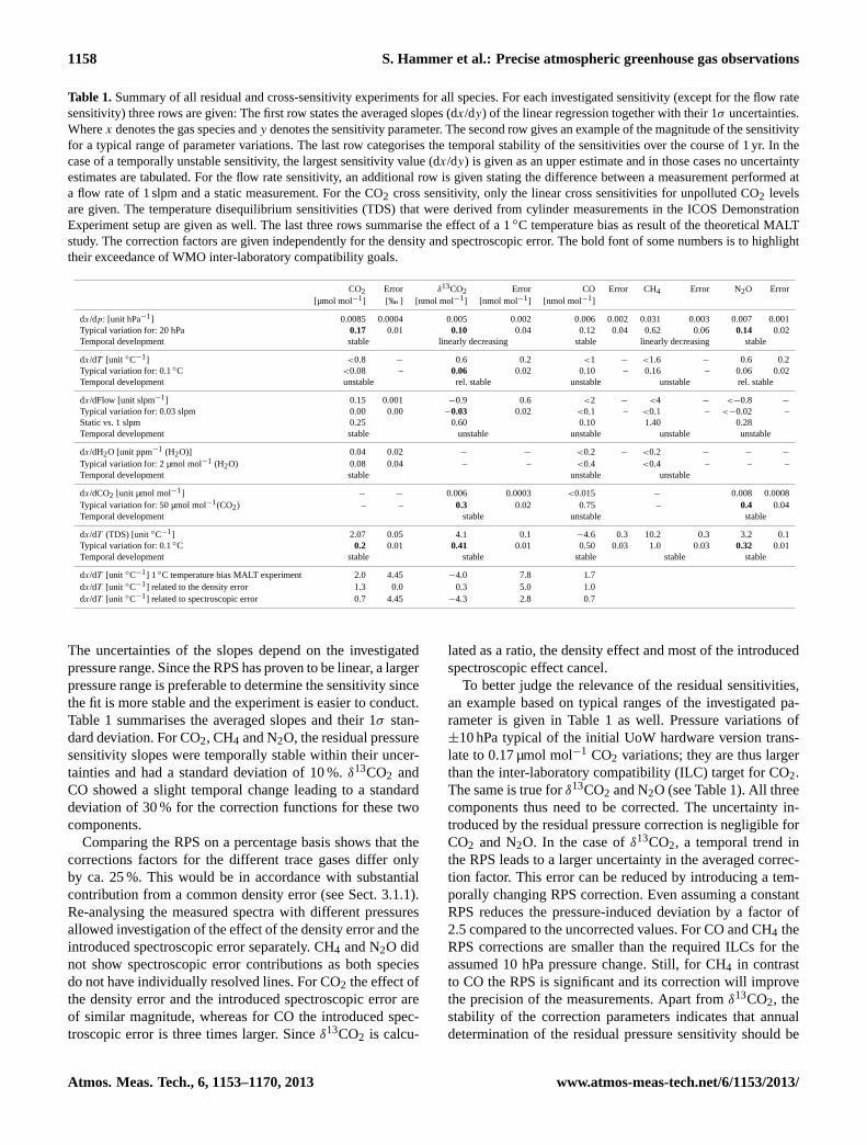
Table 1.Summary of all residual and cross-sensitivity experiments for all species. For each investigated sensitivity (except for the flow ratesensitivity) three rows are given: The first row states the averaged slopes (dx/dy) of the linear regression together with their 1σ uncertainties.Wherex denotes the gas species andy denotes the sensitivity parameter. The second row gives an example of the magnitude of the sensitivityfor a typical range of parameter variations. The last row categorises the temporal stability of the sensitivities over the course of 1 yr. In thecase of a temporally unstable sensitivity, the largest sensitivity value (dx/dy) is given as an upper estimate and in those cases no uncertaintyestimates are tabulated. For the flow rate sensitivity, an additional row is given stating the difference between a measurement performed ata flow rate of 1 slpm and a static measurement. For the CO2 cross sensitivity, only the linear cross sensitivities for unpolluted CO2 levelsare given. The temperature disequilibrium sensitivities (TDS) that were derived from cylinder measurements in the ICOS DemonstrationExperiment setup are given as well. The last three rows summarise the effect of a 1◦C temperature bias as result of the theoretical MALTstudy. The correction factors are given independently for the density and spectroscopic error. The bold font of some numbers is to highlighttheir exceedance of WMO inter-laboratory compatibility goals.

CO2 Error δ13CO2 Error CO Error CH4 Error N2O Error[µmol mol−1] [‰ ] [nmol mol−1] [nmol mol−1] [nmol mol−1]

dx/dp: [unit hPa−1] 0.0085 0.0004 0.005 0.002 0.006 0.002 0.031 0.003 0.007 0.001Typical variation for: 20 hPa 0.17 0.01 0.10 0.04 0.12 0.04 0.62 0.06 0.14 0.02Temporal development stable linearly decreasing stable linearly decreasing stable

dx/dT [unit ◦C−1] <0.8 − 0.6 0.2 <1 − <1.6 − 0.6 0.2Typical variation for: 0.1◦C <0.08 – 0.06 0.02 0.10 – 0.16 – 0.06 0.02Temporal development unstable rel. stable unstable unstable rel. stable

dx/dFlow [unit slpm−1] 0.15 0.001 −0.9 0.6 <2 − <4 − <−0.8 −

Typical variation for: 0.03 slpm 0.00 0.00 −0.03 0.02 <0.1 – <0.1 – <−0.02 –Static vs. 1 slpm 0.25 0.60 0.10 1.40 0.28Temporal development stable unstable unstable unstable unstable

dx/dH2O [unit ppm−1 (H2O)] 0.04 0.02 − − <0.2 − <0.2 − − −

Typical variation for: 2 µmol mol−1 (H2O) 0.08 0.04 – – <0.4 <0.4 – – –Temporal development stable unstable unstable

dx/dCO2 [unit µmol mol−1] − − 0.006 0.0003 <0.015 − 0.008 0.0008Typical variation for: 50 µmol mol−1(CO2) – – 0.3 0.02 0.75 – 0.4 0.04Temporal development stable unstable stable

dx/dT (TDS) [unit ◦C−1] 2.07 0.05 4.1 0.1 −4.6 0.3 10.2 0.3 3.2 0.1Typical variation for: 0.1◦C 0.2 0.01 0.41 0.01 0.50 0.03 1.0 0.03 0.32 0.01Temporal development stable stable stable stable stable

dx/dT [unit ◦C−1] 1 ◦C temperature bias MALT experiment 2.0 4.45 −4.0 7.8 1.7dx/dT [unit ◦C−1] related to the density error 1.3 0.0 0.3 5.0 1.0dx/dT [unit ◦C−1] related to spectroscopic error 0.7 4.45 −4.3 2.8 0.7

The uncertainties of the slopes depend on the investigatedpressure range. Since the RPS has proven to be linear, a largerpressure range is preferable to determine the sensitivity sincethe fit is more stable and the experiment is easier to conduct.Table 1 summarises the averaged slopes and their 1σ stan-dard deviation. For CO2, CH4 and N2O, the residual pressuresensitivity slopes were temporally stable within their uncer-tainties and had a standard deviation of 10 %.δ13CO2 andCO showed a slight temporal change leading to a standarddeviation of 30 % for the correction functions for these twocomponents.

Comparing the RPS on a percentage basis shows that thecorrections factors for the different trace gases differ onlyby ca. 25 %. This would be in accordance with substantialcontribution from a common density error (see Sect. 3.1.1).Re-analysing the measured spectra with different pressuresallowed investigation of the effect of the density error and theintroduced spectroscopic error separately. CH4 and N2O didnot show spectroscopic error contributions as both speciesdo not have individually resolved lines. For CO2 the effect ofthe density error and the introduced spectroscopic error areof similar magnitude, whereas for CO the introduced spec-troscopic error is three times larger. Sinceδ13CO2 is calcu-

lated as a ratio, the density effect and most of the introducedspectroscopic effect cancel.

To better judge the relevance of the residual sensitivities,an example based on typical ranges of the investigated pa-rameter is given in Table 1 as well. Pressure variations of±10 hPa typical of the initial UoW hardware version trans-late to 0.17 µmol mol−1 CO2 variations; they are thus largerthan the inter-laboratory compatibility (ILC) target for CO2.The same is true forδ13CO2 and N2O (see Table 1). All threecomponents thus need to be corrected. The uncertainty in-troduced by the residual pressure correction is negligible forCO2 and N2O. In the case ofδ13CO2, a temporal trend inthe RPS leads to a larger uncertainty in the averaged correc-tion factor. This error can be reduced by introducing a tem-porally changing RPS correction. Even assuming a constantRPS reduces the pressure-induced deviation by a factor of2.5 compared to the uncorrected values. For CO and CH4 theRPS corrections are smaller than the required ILCs for theassumed 10 hPa pressure change. Still, for CH4 in contrastto CO the RPS is significant and its correction will improvethe precision of the measurements. Apart fromδ13CO2, thestability of the correction parameters indicates that annualdetermination of the residual pressure sensitivity should be



45

1

2

3

4

Figure 2. a) Residual pressure sensitivity (RPS) for CO2 measured on 20th

and 22nd

of June, 5

2011. Small and wide pressure ranges are shown together with a common linear fit. Individual 6

errors are smaller than the symbols. b) Temporal stability of the slope of the residual pressure 7

sensitivity for CO2. The mole fractions of the used cylinders were all in the range of ambient 8

concentrations in Heidelberg. 9

10

Fig. 2. (a) Residual pressure sensitivity (RPS) for CO2 measuredon 20 and 22 June 2011. Small and wide pressure ranges are showntogether with a common linear fit. Individual errors are smaller thanthe symbols.(b) Temporal stability of the slope of the residual pres-sure sensitivity for CO2. The mole fractions of the used cylinderswere all in the range of ambient concentrations in Heidelberg.

sufficient to take into account systematic long-term drifts ofthe RPSs. The underlying cause of the drift in theδ13CO2RPS correction parameter is not yet understood. Temporaldrifts in the calibration of the pressure sensor would causea systematic drift in the correction parameters of all speciesexceptδ13CO2.

For the instrument versions after the ICOS demonstrationsetup the pressure is controlled to� 1 hPa and pressure cor-rections become very small or negligible. In the IUP instru-mental setup, a potential drift of the pressure sensor can ad-ditionally be controlled by the second pressure sensor in theadditional EPC.

3.4 Temperature sensitivities

3.4.1 Residual temperature sensitivity (RTS)

Compared to the RPS, the residual temperature sensitivity(RTS) has the additional complication that we do not mea-sure thetrue mean sample temperature with one tempera-ture sensor (see Appendix A). The RTD sensor used in theICOS Demonstration Experiment setup was placed near theoutlet of the cell, whilst the thermocouple used from the in-termediate setup onwards was located in the middle of thecell. The sample temperature distribution within the cell de-pends on at least three parameters: (a) the set temperatureof the enclosure, (b) the sample temperature when enteringthe cell, and (c) the sample flow rate. In total, six dedicatedRTS experiments were performed for all species. In orderto investigate the RTS, the temperature of the cell enclosurewas varied either in its normal operational range, i.e. between29.9◦C and 30.1◦C, or in a wider range from 29.7◦C to

30.3◦C. For each set temperature step we allowed enoughtime for the spectrometer and the sample cell to equilibrate.In our setups this took roughly 60 to 90 min, based on theCO2 variability. For CO2, N2O andδ13CO2, linear residualtemperature sensitivities were observed in each experiment.Although each experiment showed good linear relations forCO2, the slopes varied substantially and even changed signafter six months. For N2O andδ13CO2 the RTS was stablewithin 30 % for all experiments. The residual temperaturesensitivity for CO and CH4 was weak, not temporally stableand only for some experiments a distinct relation to cell tem-perature was observed. The averaged RTS slopes and theirstandard deviations are given in Table 1. For better classifi-cation of the results, an example based on observed peak-to-peak temperature variability of 0.1◦C is listed in Table 1 aswell. When considering the ILC targets, only the observedRTS forδ13CO2 is significant and needs to be corrected.

In order to investigate the effect of the initial sample tem-perature on the cell temperature, we conducted an experi-ment where a cylinder was first measured at room temper-ature before the entire cylinder was cooled to zero degreesCelsius and measured again. The cell temperature as wellas the measured mole fractions did, however, not change inthis experiment. This implies that the residence time of thesample in the inlet and drying system, i.e. the Nafion dryer,is sufficient to compensate for at least a 30◦C temperaturedifference of the incoming sample.

3.4.2 Temperature disequilibrium sensitivity (TDS)

The temperature disequilibrium sensitivity (TDS) describedin this subsection is related to the RTD temperature sensorused in the UoW and the ICOS Demonstration Experimentsetup. These findings resulted in a replacement of the RTDtemperature sensor with a J-type thermocouple from the in-termediate setup onwards.

Using the RTD sensor, stronger temperature sensitivitieswere present in all cylinder gas measurement records, imply-ing that temperature is one of the key parameters to performprecise calibration measurements. In the course of the ICOSDemonstration Experiment, the in situ FTIR analyser wasset up in different laboratories under different environmen-tal conditions, i.e. averaged laboratory temperatures rangedfrom 17 to 27◦C. Although the enclosure temperature wasstable at 30.00±0.05◦C at all locations, cell temperaturevaried slightly and was anti-correlated with laboratory tem-perature. Figure 3 shows the deviations from the averagedmole fraction of the 24- to 48-hourly measured sub-targettank with respect to the cell temperature. The other simul-taneously measured cylinders, two calibration gases and theregular target gas, show similar temperature dependencies.We will further refer to this effect as the temperature dise-quilibrium sensitivity (TDS).

The observed TDSs for cylinder measurements are muchlarger than the RTSs, which were derived from the dedicated



46

1

2

Figure 3. Temperature disequilibrium sensitivity (TDS) of the sub-target measurements, 3

shown as deviation from mean mole fractions. Values have been corrected for all residual 4

sensitivities except for residual temperature, but not calibrated. The three different 5

temperature ranges in the cell result from different laboratory temperatures at the remote field 6

stations and in the IUP laboratory that are indicated in the top panel. The dashed lines 7

correspond to a TDS for a 1°C bias in sample temperature determination, based on the density 8

and the introduced-spectroscopic error only. Please refer to the text for more details. 9

10

11

Fig. 3. Temperature disequilibrium sensitivity (TDS) of the sub-target measurements, shown as deviation from mean mole fractions.Values have been corrected for all residual sensitivities except forresidual temperature, but not calibrated. The three different temper-ature ranges in the cell result from different laboratory temperaturesat the remote field stations and in the IUP laboratory that are indi-cated in the top panel. The dashed lines correspond to a TDS for a1◦C bias in sample temperature determination, based on the densityand the introduced spectroscopic error only. Please refer to the textfor more details.

temperature experiments described in Sect. 3.4.1. The slopesof the linear TDS and their uncertainties are summarised inTable 1 as well. For the typical temperature range of 0.1◦C,the effect is significantly larger than the ILC goals for CO2,δ13CO2 and N2O. A possible cause for the difference be-tween the two temperature sensitivity results may arise fromdifferent conditions of the instrument. While in the dedi-cated RTS experiments sample air was continuously flushedthrough the cell, each cylinder measurement, performed un-der standard operating conditions, comprises evacuation ofthe cell prior to the measurement in flow mode (Appendix A).The evacuation of the cell causes adiabatic cooling on the or-der of 5◦C. Although this adiabatic cooling effect is compen-sated for during the re-filling of the cell, the slow response ofthe RTD sensor, caused by its large thermal mass, leads to abiased temperature measurement, even after the sample tem-perature has recovered. In the UoW and ICOS demonstrationexperiment setup the evacuation-induced temperature devia-tion was further amplified by the fact that the sensor of the ac-tive enclosure temperature control was mounted directly on

the cell walls. The adiabatic cooling thus disturbed the tem-perature equilibrium in the enclosure, leading to a feedback-loop of the active temperature control.

To investigate if the TDS can be explained by a biasedsample temperature measurement we examined the influenceof a 1◦C temperature bias on the retrieved concentrations ofa synthetic absorption spectrum. This allows separating theimpact of the density error from the introduced spectroscopicerror. The line shape error does not show up in such a study.The theoretical temperature bias correction parameters arelisted in Table 1 and shown in Fig. 3 as dashed black lines.The theoretical temperature sensitivity of an assumed tem-perature bias of 1◦C agrees well with the observed TDS forall species. Only for N2O the theoretical temperature sensi-tivity is smaller than the observed TDS.

This result gives strong evidence for biased sample tem-perature measurements after an evacuation process. The TDSwas the main reason to replace the RTD sensor with a fasterresponding thermocouple. Such thermocouples have becomethe standard temperature sensor from the intermediate setuponwards. In addition, we moved the sensor of the active en-closure temperature control out of direct contact with the cellwall. With these measures, the TDS was no longer observedfor cylinder measurements.

For all cylinder measurements performed with the ICOSDemonstration Experiment setup, we use the TDS correctionparameters derived from the sub-target gas measurements tocorrect all our standard and target gas measurements. Theanti-correlated relation between room and cell temperatureis most likely caused by an overcompensation of the activeenclosure temperature control.

3.5 Flow rate sensitivity

Neither the spectroscopic nor the mole fraction determina-tions have a direct link to the sample flow rate through thecell. The flow rate has only an indirect effect through thetemperature distribution in the cell. Thus we expect the flowrate sensitivity to be small compared to the temperature sen-sitivity. Nevertheless, the flow rate sensitivity was investi-gated in three dedicated experiments, mainly motivated fromthe observed difference between a constantly flushed and aclosed-off cell. Apart from CO, the measured mole fractionsare always higher in a closed off cell than in a constantlyflushed cell. Under our standard operating conditions this ef-fect can be as large as 0.25 µmol mol−1 for CO2, 0.6 ‰ forδ13CO2, −0.1 nmol mol−1 for CO, 1.4 nmol mol−1 for CH4and 0.28 nmol mol−1 for N2O. We hypothesise that the ob-served difference between static and dynamic measurementsis caused by different temperature distributions in the cell.

The observed flow sensitivity in the range between 0.8 and1.2 slpm could be linearly approximated, however the linear-ity broke down when approaching zero flow. As expected, theflow sensitivities are small. In addition to this, the gas-flowthrough the cell was very stable due to the additional sample



47

1

2

3

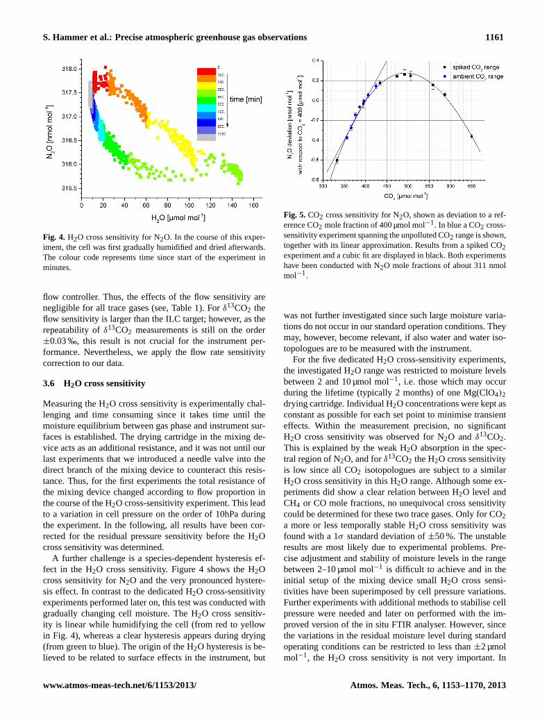
Figure 4. H2O cross sensitivity for N2O. In the course of this experiment the cell was first 4

gradually humidified and dried afterwards. The colour code represents time since start of the 5

experiment in minutes. 6

7

Fig. 4. H2O cross sensitivity for N2O. In the course of this exper-iment, the cell was first gradually humidified and dried afterwards.The colour code represents time since start of the experiment inminutes.

flow controller. Thus, the effects of the flow sensitivity arenegligible for all trace gases (see, Table 1). Forδ13CO2 theflow sensitivity is larger than the ILC target; however, as therepeatability ofδ13CO2 measurements is still on the order±0.03 ‰, this result is not crucial for the instrument per-formance. Nevertheless, we apply the flow rate sensitivitycorrection to our data.

3.6 H2O cross sensitivity

Measuring the H2O cross sensitivity is experimentally chal-lenging and time consuming since it takes time until themoisture equilibrium between gas phase and instrument sur-faces is established. The drying cartridge in the mixing de-vice acts as an additional resistance, and it was not until ourlast experiments that we introduced a needle valve into thedirect branch of the mixing device to counteract this resis-tance. Thus, for the first experiments the total resistance ofthe mixing device changed according to flow proportion inthe course of the H2O cross-sensitivity experiment. This leadto a variation in cell pressure on the order of 10hPa duringthe experiment. In the following, all results have been cor-rected for the residual pressure sensitivity before the H2Ocross sensitivity was determined.

A further challenge is a species-dependent hysteresis ef-fect in the H2O cross sensitivity. Figure 4 shows the H2Ocross sensitivity for N2O and the very pronounced hystere-sis effect. In contrast to the dedicated H2O cross-sensitivityexperiments performed later on, this test was conducted withgradually changing cell moisture. The H2O cross sensitiv-ity is linear while humidifying the cell (from red to yellowin Fig. 4), whereas a clear hysteresis appears during drying(from green to blue). The origin of the H2O hysteresis is be-lieved to be related to surface effects in the instrument, but

48

1

2

3

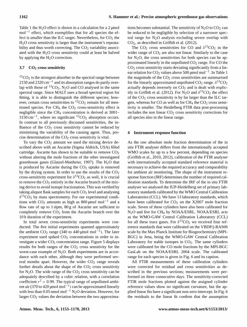
Figure 5. CO2 cross sensitivity for N2O, shown as deviation to a reference CO2 mole fraction 4

of 400 µmol mol-1

. In blue a CO2 cross sensitivity experiment spanning the unpolluted CO2 5

range is shown, together with its linear approximation. Results from a spiked CO2 experiment 6

and a cubic fit are displayed in black. Both experiments have been conducted with N2O mole 7

fractions of about 311 nmol mol-1

. 8

9

Fig. 5. CO2 cross sensitivity for N2O, shown as deviation to a ref-erence CO2 mole fraction of 400 µmol mol−1. In blue a CO2 cross-sensitivity experiment spanning the unpolluted CO2 range is shown,together with its linear approximation. Results from a spiked CO2experiment and a cubic fit are displayed in black. Both experimentshave been conducted with N2O mole fractions of about 311 nmolmol−1.

was not further investigated since such large moisture varia-tions do not occur in our standard operation conditions. Theymay, however, become relevant, if also water and water iso-topologues are to be measured with the instrument.

For the five dedicated H2O cross-sensitivity experiments,the investigated H2O range was restricted to moisture levelsbetween 2 and 10 µmol mol−1, i.e. those which may occurduring the lifetime (typically 2 months) of one Mg(ClO4)2drying cartridge. Individual H2O concentrations were kept asconstant as possible for each set point to minimise transienteffects. Within the measurement precision, no significantH2O cross sensitivity was observed for N2O andδ13CO2.This is explained by the weak H2O absorption in the spec-tral region of N2O, and forδ13CO2 the H2O cross sensitivityis low since all CO2 isotopologues are subject to a similarH2O cross sensitivity in this H2O range. Although some ex-periments did show a clear relation between H2O level andCH4 or CO mole fractions, no unequivocal cross sensitivitycould be determined for these two trace gases. Only for CO2a more or less temporally stable H2O cross sensitivity wasfound with a 1σ standard deviation of±50 %. The unstableresults are most likely due to experimental problems. Pre-cise adjustment and stability of moisture levels in the rangebetween 2–10 µmol mol−1 is difficult to achieve and in theinitial setup of the mixing device small H2O cross sensi-tivities have been superimposed by cell pressure variations.Further experiments with additional methods to stabilise cellpressure were needed and later on performed with the im-proved version of the in situ FTIR analyser. However, sincethe variations in the residual moisture level during standardoperating conditions can be restricted to less than±2 µmolmol−1, the H2O cross sensitivity is not very important. In



Table 1 the H2O effect is shown in a calculation for a 2 µmolmol−1 effect, which exemplifies that for all species the ef-fect is smaller than the ILC target. Nevertheless, for CO2 theH2O cross sensitivity is larger than the instrument’s repeata-bility and thus worth correcting. The CO2 variability associ-ated with the H2O cross sensitivity could at least be halvedby applying the H2O correction.

3.7 CO2 cross sensitivity

12CO2 is the strongest absorber in the spectral range between2150 and 2320 cm−1 and its absorption ranges do partly over-lap with those of13CO2, N2O and CO analysed in the samespectral range. Since MALT uses a broad spectral region forfitting, it is able to distinguish the different species; how-ever, certain cross sensitivities to12CO2 remain for all men-tioned species. For CH4 the CO2 cross-sensitivity effect isnegligible since the CH4 concentration is derived at 3001–3150 cm−1, where no significant12CO2 absorption occurs.In contrast to all previously discussed sensitivities, the in-fluence of the CO2 cross sensitivity cannot be reduced byminimising the variability of the causing agent. Thus, pre-cise determination of the CO2 cross sensitivity is vital.

To vary the CO2 amount we used the mixing device de-scribed above with an Ascarite (Sigma Aldrich, USA) filledcartridge. Ascarite has shown to be suitable to remove CO2without altering the mole fractions of the other investigatedgreenhouse gases (Glatzel-Mattheier, 1997). The H2O thatis produced by Ascarite during the CO2 uptake is removedby the drying system. In order to use the results of the CO2cross-sensitivity experiment forδ13CO2 as well, it is crucialto remove the CO2 entirely in the Ascarite branch of the mix-ing device to avoid isotope fractionation. This was verified bytaking aliquot flask samples for each CO2 level and analysingδ13CO2 by mass spectrometry. For our experimental condi-tions with CO2 amounts as high as 800 µmol mol−1 and aflow rate of up to 1 slpm, 80 g of Ascarite are sufficient tocompletely remove CO2 from the Ascarite branch over the10 h duration of the experiment.

In total seven cross-sensitivity experiments were con-ducted. The five initial experiments spanned approximatelythe ambient CO2 range (340 to 440 µmol mol−1). The laterexperiment used spiked CO2 concentrations in order to in-vestigate a wider CO2 concentration range. Figure 5 displaysresults for both ranges of the CO2 cross sensitivity for theworst-case example of N2O. Both experiments are in accor-dance with each other, although they were performed sev-eral months apart. However, the wider CO2 range revealsfurther details about the shape of the CO2 cross sensitivityfor N2O. The wide range of the CO2 cross sensitivity can beadequately described by a cubic relation, with a correlationcoefficientr2 > 0.99. The typical range of unpolluted ambi-ent air (370 to 420 µmol mol−1) can be approximated linearlywith less than 0.05 nmol mol−1 N2O deviation. However, forlarger CO2 values the deviation between the two approxima-

tions becomes substantial. The sensitivity of N2O to CO2 canbe reduced to be negligible by selection of a narrower spec-tral range for N2O analysis excluding severe overlap withCO2, as described in Griffith et al. (2012).

The CO2 cross sensitivities for CO andδ13CO2 in thewider range of CO2 are also not linear. Similarly to the casefor N2O, the cross sensitivities for both species can be ap-proximated linearly in the unpolluted CO2 range. For CO theCO2 cross sensitivity starts deviating significantly from a lin-ear relation for CO2 values above 500 µmol mol−1. In Table 1the magnitude of the CO2 cross sensitivities are summarisedfor the linearly approximated unpolluted CO2 range.δ13CO2actually depends inversely on CO2 and is dealt with explic-itly in Griffith et al. (2012). For N2O andδ13CO2 the effectof the CO2 cross sensitivity is by far larger than the ILC tar-gets, whereas for CO as well as for CH4 the CO2 cross sensi-tivity is smaller. The Heidelberg FTIR data post-processingincludes the non linear CO2 cross sensitivity corrections forall species also in the linear range.

4 Instrument response function

As the rawabsolutemole fraction determination of the insitu FTIR analyser differs from the internationally acceptedWMO scales by up to a few percent, depending on species(Griffith et al., 2010, 2012), calibration of the FTIR analyserwith internationally accepted standard reference material isnecessary to achieve the required accuracy and comparabilityfor ambient air monitoring. The shape of the instrument re-sponse function (IRF) determines the number of required cal-ibration standards. To determine the IRF of the in situ FTIRanalyser we analysed the IUP-Heidelberg set of primary lab-oratory standards calibrated by the WMO Central CalibrationLaboratories (CCL). We have 13 laboratory standards, whichhave been calibrated for CO2 on the X2007 mole fractionscale. Seven of these cylinders have also been calibrated forN2O and five for CH4 by NOAA/ESRL. NOAA/ESRL actsas the WMO-GAW Central Calibration Laboratory (CCL)for all these trace gases. Forδ13CO2 we received four ref-erence standards that were calibrated on the VBDP/j-RAS06scale by the Max Planck Institute for Biogeochemistry (MPI-BGC) in Jena, being the WMO-GAW Central CalibrationLaboratory for stable isotopes in CO2. The same cylinderswere calibrated for the CO mole fractions by the MPI-BGCGasLab on the NOAA/ESRL 2004 scale. The calibratedrange for each species is given in Fig. 6 and its caption.

All FTIR measurements of these calibration cylinderswere corrected for residual and cross sensitivities as de-scribed in the previous sections; measurements were per-formed on three consecutive days. The sensitivity-correctedFTIR mole fractions plotted against the assigned cylinderreference values show no significant curvature, but the ap-plied linear fits have a significant non-zero intercept. In Fig. 6the residuals to the linear fit confirm that the assumption



49

1

2

3

Figure 6. Linearity of the FTIR analyser. For each species the residual to the linear fit of the 4

externally assigned mole fractions against sensitivity-corrected FTIR mole fractions are 5

shown. The investigated mole fraction ranges are defined by the spread of the secondary 6

laboratory cylinders used for the Heidelberg GC system and are as follows: CO2: 348 to 426 7

µmol mol-1

; δ13

CO2: -12.65 to -9.55‰; CO: 90 to 620 nmol mol-1

, CH4: 1757 to 1970 nmol 8

mol-1

and N2O: 307 to 343 nmol mol-1

. 9

10

11

Fig. 6. Linearity of the FTIR analyser. For each species the resid-ual to the linear fit of the externally assigned mole fractions againstsensitivity-corrected FTIR mole fractions are shown. The investi-gated mole fraction ranges are defined by the spread of the sec-ondary laboratory cylinders used for the Heidelberg GC system andare as follows: CO2: 348 to 426 µmol mol−1; δ13CO2: −12.65 to−9.55‰ ; CO: 90 to 620 nmol mol−1; CH4: 1757 to 1970 nmolmol−1 and N2O: 307 to 343 nmol mol−1.

of linear instrument response functions is justified for allspecies. The error bars in Fig. 6 depict the combined errorof the FTIR measurement and the error of the calibrationcylinder assigned mole fractions. The standard deviationsof the residuals are 0.03 µmol mol−1 for CO2, 0.04 ‰ forδ13CO2, 0.4 nmol mol−1 for CO, 0.4 nmol mol−1 for CH4and 0.08 nmol mol−1 for N2O. From these results we canconclude that the IRFs can, in accordance with the WMOILC targets, be approximated linearly over the investigatedrange for all tracers. However, the non-zero intercepts of theregression functions prevent a simple one-point calibration,leading to a minimum of two calibration standards for theFTIR. For high-accuracy demands, as in atmospheric back-ground monitoring programs, the usage of three calibrationstandards to define the IRF is advised. A three-point cali-bration reduces the sensitivity to individual outliers and in-strument noise in the calibration measurements. In addition,the assumption of linearity for the IRF, and potential long-term changes, can routinely be tested using a goodness of thelinear fit criteria.

5 Temporal stability of the FTIR analyser andcalibration frequency

In order to assess the precision of the in situ FTIR analyser,measurement repeatability as well as reproducibility on dif-ferent time scales has to be determined. In the following,we will use the terminology related to the GAW glossary ofQA/QC (Klausen and Scheel, 2007). The issue of measure-ment stability is vital for all long-term monitoring efforts and

50

1

2

3

Figure 7. Short term stability of the FTIR components during September 2011. Minute-by-4

minute cylinder measurements over the course of six days. In grey the dry air mole fractions 5

are given (but are only visible in the case of CO2). The coloured symbols show the sensitivity 6

corrected values, with a linear fit to detect drifts. 7

8

Fig. 7.Short-term stability of the FTIR components during Septem-ber 2011. Minute-by-minute cylinder measurements over the courseof 6 days. In grey the dry-air mole fractions are given (but are onlyvisible in the case of CO2). The coloured symbols show the sensi-tivity corrected values, with a linear fit to detect drifts.

determines the required calibration frequency to reach a cer-tain level of reproducibility. In the following, we will subdi-vide the stability requirement into two parts: short term andlong term.Short termhandles drifts and other artefacts on atime scale from hours to days, whilelong termcovers weeksto months.

5.1 Short-term stability

To quantify short-term drifts of the FTIR analyser, a targetgas was continuously flushed through the cell at the stan-dard flow rate of 1 slpm for 6 days, comprising a weekend aswell as weekdays, to cover different laboratory conditions.Absorption spectra with an averaging time of 1 min wererecorded and analysed offline to avoid downtime. The respec-tive time series of the dry-air mole fractions, calculated ac-cording to Eq. (2), are shown in Fig. 7 in grey. The sensitivitycorrected results are shown as well (coloured symbols).

This short-term stability test was conducted in Septem-ber 2011 for the intermediate setup. Thus, the sample prop-erties in the cell remained fairly constant over the courseof the experiment, as expressed by their 1σ standard devia-tions:±0.01◦C for cell temperature,±0.01 hPa for cell pres-sure,±0.2 µmol mol−1 for moisture level, and±0.01 slpmfor sample flow rate. The Heidelberg laboratory temperatureoscillated between 23.2 and 25.1◦C for this period; however,the influence on cell temperature was small. The generallyvery stable sample properties in the cell lead to only smallcorrections of the residual sensitivities (Fig. 7). Only for CO2was a clear correlation to cell temperature found. The RTScorrections thus improve the CO2 standard deviation of the1 min measurements from 0.037 to 0.029 µmol mol−1 – forall other species the sensitivity corrections are marginal.



The initial 6 h of the test show a small settling-in effectfor CO2 as well as for CO. Most likely this can be attributedto adjustments of the pressure regulator of the cylinder andthe cell parameters.δ13CO2 and CH4 show a slight trendover the 6 days, persisting even after the sensitivity correc-tion with 0.02 ‰ day−1 for δ13CO2 and−0.04 nmol mol−1

day−1 for CH4. The drift in δ13CO2 might be related to afractionation effect in the fast-emptying high-pressure cylin-der; however, this cannot be proven since no pre- and post-mass-spectrometer measurements have been performed onthis cylinder.

The same data set from September 2011 (Fig. 7) can beused to determine the repeatability of the FTIR measure-ments using Allan variance analysis (Werle et al., 1993). InTable 2, the 1σ repeatability for 2.5 and 10 min averagingtime is given. An averaging time of 2.5 min is used in stan-dard operating conditions for the Heidelberg in situ FTIR(3 min measurements including 30 s online analysis time).The 10 min repeatability is given for reasons of compara-bility to the earlier results from Griffith et al. (2010, 2012).Similar to the findings by Griffith et al. (2012), the repeata-bility of all species except for CO2 initially improves with thesquare root of averaging time for at least 30 min. For longerintegration intervals the repeatability still improves, but ata slightly lower rate. For sensitivity-corrected CO2, the re-peatability improves steadily up to an averaging time of 15 h,but only by one third of the square root of time. Detailed Al-lan variance plots based on our data can be found as Fig. 4 inGriffith et al. (2012).

We determined the reproducibility for measurements av-eraged over 3 min, as given in Table 2, by pooling three1 min spectra and calculated their 1σ standard deviation. Thisreproducibility includes any potential changes or arbitrarydrifts in the spectrometer or any sensor over the investigated6-day period. The comparison of the repeatability and repro-ducibility of the 3 min averages in Table 2 emphasises theremarkably good short-term stability of the in situ FTIR.

5.2 Long-term stability of the in situ FTIR analyser

The long-term stability of the instrument response function(IRF) determines the calibration frequency as well as the cal-ibration strategy. If the IRF is absolutely stable in time, in-terpolation between repeated calibrations does not improvemeasurement accuracy. This is due to the intrinsic uncer-tainty of each calibration measurement, which is then passedon to the measurements and increases their noise. If, on theother hand, the temporal changes of the IRF are larger thanthe instrument’s repeatability, regular calibration improvesthe accuracy substantially. In the latter case the question con-cerning the required calibration frequency arises. In Sect. 5.1we showed that, compared to the noise, for CO2, CO andN2O no systematic change of residual pressure and tempera-ture sensitivity-corrected data occurred over the time scale ofup to 6 days. Here we will investigate the longer time scales,

51

1

2

3

Figure 8. CO2 target gas record in its different data processing stages. 4

5

Fig. 8.CO2 target gas record in its different data processing stages.

based on the data set we collected during the ICOS Demon-stration Experiment. During these field campaigns, 24- and48-hourly calibrations were performed with two standardcylinders, covering a suitable mole fraction range for all fivecomponents. In between the calibrations, a so-called target orsurveillance tank was measured for quality control. In termsof sensitivity correction and calibration, the target cylinderwas analysed in a similar way as any unknown sample froma cylinder. In the next section we will revisit the influence ofthe residual and cross sensitivities discussed in section 3 onthe example of the CO2 long-term target record.

5.2.1 Influence of the CO2 residual and crosssensitivities on long-term records

Figure 8 displays the deviations of the CO2 target measure-ment from the mean mole fraction over the different evalu-ation stages from the raw FTIR measurements to the finallycalibrated data. Each target gas value consists of the averageand the standard deviation of five sequentially recorded 3 minspectra. The dry-air mole fractions as calculated by MALTare shown in blue; they exhibit step changes as well as grad-ual changes. The 1σ standard deviation for the CO2 targetgas is 0.25 µmol mol−1 with a peak to peak variability of0.8 µmol mol−1 over this 5-month measurement period. Theprominent changes in the dry-air mole fraction can be relatedto changes in cell temperature and pressure, caused by chang-ing laboratory conditions and/or a degradation of the flowcontroller that was additionally installed during the ICOSDemonstration Experiment. Correction for residual and crosssensitivities determined in Sect. 3 improves the reproducibil-ity of the 24- to 48-hourly values as well as the 1σ scatterover the whole period by a factor of two to only 0.11 µmolmol−1 (red dots in Fig. 8). The residual and cross sensi-tivity correction takes care of most of the pronounced stepchanges; however, some outliers are persistent (e.g. in mid-July) and can thus not be explained by a change in one of our



Table 2. Repeatability (1σ ) for 2.5 and 10 min averaging times deduced from Allan-Variance analysis. Reproducibility (1σ) for 3 minmeasurements of a single tank over a 6-day period and target gas reproducibility over the course of several months (compare Fig. 9). Totaluncertainty for a single ambient air measurement (see Sect. 6).

Total uncertainty incl.Species Repeatability (1σ) Reproducibility (1σ) errors in sensitivities (1σ)

Time 2.5 10 Single tank Target: Inter- Target: Singleperiod min min 6 days, 3 min mediate setup IUP setup measurement

CO2 [µmol mol−1] 0.018 0.012 0.023 0.043 0.016 0.032δ13CO2 [‰ ] 0.05 0.03 0.06 0.062 0.034 0.07CH4 [nmol mol−1] 0.2 0.1 0.2 0.21 0.12 0.25CO [nmol mol−1] 0.2 0.1 0.2 0.26 0.11 0.22N2O [nmol mol−1] 0.07 0.04 0.07 0.042 0.042 0.084

investigated residual and cross sensitivities. The variabilityin the sensitivity-corrected target gas measurements is stilllarger than the observed short-term repeatability expressedby the error bars and investigated in Sect. 3. In addition, theCO2 variability still shows long-term changes and outliers.Thus, applying regular, e.g. daily, calibration might help toreduce the CO2 variability further. By using a linear inter-polation between the 24- to 48-hourly calibration measure-ments to determine the IRF, the 1σ standard deviation of theCO2 target measurements is reduced to±0.05 µmol mol−1,as shown by black squares in Fig. 8.

Although the calibrated measurements are generally satis-fying the WMO compatibility goal of±0.1 µmol mol−1 forCO2 measurements in the Northern Hemisphere, individualmeasurement periods show much more scatter (e.g. in July).Outliers in the target gas record (July 2011) are caused bybad calibration measurements. The impact of a single cali-bration measurement depends largely on the strategy chosento derive the IRF. We therefore investigated different cali-bration strategies such as (a) averaged IRF, (b) interpolatedIRF between smoothed (e.g. moving weekly median) calibra-tion measurements, and (c) interpolated IRF between neigh-bouring calibration measurements. Based on the repeatabil-ity of the target cylinder measurements, strategy (c) yieldedthe best results, although its sensitivity to single bad cali-bration measurements is largest. Careful selection of cali-bration outliers is thus recommended to minimise artefactsin the time series. For all following results we used calibra-tion strategy (c), which is the linear interpolation of the IRFbetween neighbouring calibration measurements.

5.2.2 Long-term reproducibility for all species

Figure 9 comprises the sensitivity-corrected and calibratedtarget gas measurements for all components. In Septem-ber 2011 the FTIR system was modified to the interme-diate setup. The long-term reproducibility of the ICOSDemonstration Experiment setup can be judged based on the1σ standard deviations up to September 2011:±0.06 µmol

52

1

2

3

Figure 9. Long term stability of the FTIR analyser based on the 24- to 48-hourly target gas 4

measurements. Vertical gray lines denote location changes of the instrument to Cabauw the 5

Netherlands (CBW) and Houdelaincourt, France (OPE). The gray shaded area highlights a 6

period with less stable cell pressure. Red shaded areas mark instrument down times due to 7

modifications and/or laser failure. In September 2011 the internal mass flow controller and 8

end of November 2011 the electronic pressure controller (EPC) was installed. The dashed 9

black line indicates the change in standard operation conditions from then on no evacuation 10

was performed during sample exchange. 11

12

Fig. 9.Long-term stability of the FTIR analyser based on the 24- to48-hourly target gas measurements. Vertical grey lines denote loca-tion changes of the instrument to Cabauw, the Netherlands (CBW),and Houdelaincourt, France (OPE). The grey shaded area highlightsa period with less-stable cell pressure. Red shaded areas mark in-strument down times due to modifications and/or laser failure. InSeptember 2011 the internal mass flow controller was installed,and at the end of November 2011 the electronic pressure controller(EPC). The dashed black line indicates the change in standard oper-ation conditions – from then on no evacuation was performed duringsample exchange.

mol−1 for CO2, ±0.05 ‰ for δ13CO2, ±0.45 nmol mol−1

for CO,±0.28 nmol mol−1 for CH4 and±0.1 nmol mol−1

for N2O. The 1σ standard deviations are thus close to orwithin the ILC targets for all trace gases (WMO, 2011). Forδ13CO2 the reproducibility of±0.05 ‰ is acceptable, keep-ing in mind that the in situ FTIR analyser is one of the first in-struments delivering continuousδ13CO2 measurements. TheWMO-GAW requested target compatibility forδ13CO2 is±0.01 ‰, and yet only met by very few mass spectrometerlaboratories (Huang et al., 2011).

No significant drift was observed for any species. Thesmall step change in CO is not explained by any of the inves-tigated sensitivities. Re-calibration of the working standards



as well as the target tank at the Max Planck Institute for Bio-geochemistry confirmed that neither the target cylinder northe calibration cylinders drifted in any of the investigatedspecies.

For CO2 it is obvious that the performance of the in situFTIR analyser declined after middle of June 2011. Check-ing the FTIR parameters revealed that from middle of Juneonwards, the standard deviation of the sample pressure in-creased from better than±2 hPa to more than±7 hPa. Thisincrease was most likely caused by a progressive degrada-tion of the additionally installed external mass flow con-troller (blue MFC in Fig. 1). In Sect. 3.3 we have shownthat the largest pressure sensitivity corrections are found forCO2; consequently, we observe the largest deviation betweenthe short and long-term reproducibility for CO2. The de-crease in reproducibility for CO is caused by the step changeon 15 June (compare Fig. 9) and for N2O by several outliers.

The first red shaded area in Fig. 9 marks the re-building ofthe instrument to the intermediate setup. The reproducibilityderived with this instrument configuration is given in Table 2.The largest improvement compared to the ICOS Demonstra-tion Experiment setup, a factor of 2, was achieved for N2O,improving the in situ FTIR analyser precision to well belowthe ILC target. The performance for CO2, δ13CO2 and CH4remains at a comparably good level. The drift, which was ob-served for CO, is caused by a drifting calibration gas cylinderbeing used during this time. Uncalibrated results suggest thatthe CO reproducibility improved as well.

To decouple sample pressure and flow, and to ease samplehandling, an additional electronic pressure controller (EPC)(El-Press, Bronkhorst, The Netherlands) was installed at theinlet of the cell in the IUP setup. In Fig. 9 the target gas mea-surements performed with this new configuration are shownafter the second red shaded area. The reproducibility of thesensitivity-corrected and -calibrated target gas results is alsosummarised in Table 2. The introduction of the additionalEPC improved the reproducibility of all components exceptfor N2O by approximately a factor of two. The dashed linein Fig. 9 in mid-December 2011 indicates a change in ourstandard operating conditions. From there on we skipped theevacuation step during sample exchange and used the flush-ing approach (refer to Appendix A). This was done in orderto investigate the benefits of not disrupting the temperatureand moisture equilibrium in the cell by the evacuation. InFig. 9 no significant difference between both sample change-over strategies is visible. Thus, after two months we changedback to our SOC to save calibration gas and to shorten thecalibration measurement interval. This finding depends onthe temperature sensor type used. It will most likely not bevalid for the slow-responding RTD temperature sensor.

In the final IUP setup short and long-term reproducibilityare similar for all components (see Table 2). These resultsdemonstrate that the long-term stability of the in situ FTIRanalyser is suitable for background air monitoring if mea-

53

1

2

3

Figure 10. Calibration frequency test. 1σ standard deviation of the target gas measurements as 4

a function of days between calibrations. Open symbols represent less stable instrument 5

conditions with sample pressure variations (1σ) of more than ±7 hPa. Filled symbols relate to 6

stable conditions with sample pressure variations (1σ) of less than ±2 hPa. 7

8

Fig. 10. Calibration frequency test. 1σ standard deviation of thetarget gas measurements as a function of days between calibrations.Open symbols represent less-stable instrument conditions with sam-ple pressure variations (1σ) of more than±7 hPa. Filled symbolsrelate to stable conditions with sample pressure variations (1σ) ofless than±2 hPa.

surements are calibrated and properly corrected for residualand cross sensitivities.

5.3 Calibration frequency

The target gas record can further be used to estimate the in-fluence of the calibration frequency on the reproducibility.In Fig. 9 we used the highest calibration frequency of 24- to48- hourly calibrations with two standard gases. With the tar-get gas data set, we can investigate the influence of stepwiseprolonged calibration intervals on the 1σ reproducibility ofthe results. Since, especially for CO2, the performance of theFTIR analyser can be separated into two periods – stable andless-stable conditions (compare grey shaded area in Fig. 9) –we will evaluate the calibration frequency test for both sta-bility conditions separately. The less-stable period, withoutproper control of the additional MFC introduced in the ICOSDemonstration Experiment setup, the instrument configura-tion is comparable to the initial UoW setup.

In each panel of Fig. 10 the relation between 1σ repro-ducibility and calibration frequency is plotted. Closed sym-bols represent stable instrument conditions with a cell pres-sure variability of less than±2 hPa, open symbols show less-stable conditions; here, the cell pressure variability was fourtimes larger. Under stable instrument conditions the 1σ targetreproducibility of CO2 was better than±0.03 µmol mol−1

for 24- to 48-hourly calibrations. Prolonging the calibrationfrequency even to 2 or 3 months changes the reproducibilityonly slightly to 0.05 µmol mol−1. During less-stable instru-ment conditions, the reproducibility improves steadily withincreasing calibration frequency; however, even 24- to 48-hourly calibrations do not result in the reproducibility ofthe stable conditions. It seems that under less-stable condi-tions, substantial variations occur on sub-daily time scales,



for example during the campaign in OPE the laboratory tem-perature changed by 10◦C within 1 day.

The other trace species, apart from N2O, show a similarbehaviour to that of CO2, although the difference betweenstable and less-stable instrument conditions is not as pro-nounced. For the highest calibration frequency, the achievedreproducibility is on par or even better than the short-termreproducibility determined in Sect. 5.1. This is caused by thefact that the investigated target measurements as well as thecalibration measurements are averaged values of five indi-vidual spectra reducing the scatter by a factor of

√5. This

implies that for a single 3 min ambient air measurement thereproducibility is a factor of

√5 larger than the one shown

for the target measurements. In contrast to the IRF of othergases, the IRF for N2O has two large-step changes duringthe stable instrument conditions (not shown) leading to theinverse results in the calibration frequency investigation. Therecorded sample and instrument properties give no evidencethat could explain the step changes in the N2O IRF.

Increasing the calibration frequency from weekly to 24- or48-hourly improves the reproducibility on average by 20 %for all gases. Depending on the specific accuracy needs,weekly calibrations should be sufficient and beneficial forcalibration gas consumption as well.

6 Error assessment for ambient air measurement

Different sources of error contribute to the total error ofan individual ambient air measurement. These error con-tributions are partly systematic and partly random and canoften not easily be separated. Obvious error contributionarises from (a) measurement repeatability, (b) uncertaintiesin residual and cross-sensitivity corrections, (c) uncertain-ties introduced by the two-point calibration, and (d) uncer-tainty of the assigned mole fraction of the calibration cylin-ders themselves.

These error sources are not independent from each other.For example, the uncertainties originating from (a) and(b) (repeatability and the residual and cross-sensitivity cor-rections) feed directly into the uncertainty introduced by theregular calibration. Thus, a combined uncertainty compris-ing (a), (b) and (c) can be derived from the reproducibilityof the target measurements as listed in Table 2. However, thetarget measurement reproducibility is derived from averagedvalues and has thus to be multiplied by a factor of

√5 (since

there are 5 target measurements). For ambient air measure-ments the uncertainties of the CO2 cross sensitivities must beadded since this error component is not present in the targetmeasurements. The total uncertainties are thus given in thelast column of Table 2. The contribution of the uncertaintiesof the assigned values of the calibration cylinders is an addi-tional, systematic error component that has to be accountedfor separately.

7 Conclusions and outlook

The modified in situ FTIR spectrometer is well suited forGHG monitoring and fulfils the precision, accuracy and sta-bility needs for CO2, CO, CH4 and N2O measurements atbackground sites. The reproducibility forδ13CO2 does notformally fulfil the ILC targets set by WMO-GAW; how-ever, 0.03 ‰ target reproducibility (0.07 ‰ single measure-ment) is still very good for a continuously measuring in-strument. The final IUP setup of the in situ FTIR is addi-tionally equipped with an internal EPC and MFC to controlsample pressure and flow rate. To improve the temperaturemeasurement the RTD sensor was replaced by a thermocou-ple that is located in the middle of the cell to improve therepresentativeness of the measurement. These improvementslead to a factor-of-two-better repeatability for all species.In the IUP setup the effects of the residual pressure sensi-tivity and flow rate-sensitivity are negligible. The same istrue for the H2O cross sensitivity since the residual mois-ture variations can be restricted to only a few µmol mol−1 ofH2O. Reducing the causes of variability is always superior toany post-processing correction. However, for those param-eters where this is not possible, e.g. CO2 cross sensitivity,precise determination of these parameters is essential. Cur-rently, the largest remaining issue is related to the ability ofmeasuring thetrue sample temperature in the cell. Resolv-ing this temperature problem might allow for measuring cal-ibration and target gas cylinders in static mode, which wouldreduce the gas consumption by a factor of five. Measuringthe sample temperature at multiple locations could be a firststep towards improving the representativeness of the tem-perature measurement. The small Reynolds number in thecell (≈10, see Appendix A) for our standard operating con-ditions constitutes a more general problem. Improved sam-ple delivery to the cell that increases turbulence would helpminimizing temperature gradients within the cell. We alsorecommend placing the Nafion drier inside the temperature-controlled enclosure since it is important for thermal samplepre-conditioning.

The instrument has proven to be acceptably linear for allcomponents in the ambient concentration range (also for non-background conditions); however, the instrument responsefunctions have a non-zero offset for all components, imply-ing the need for at least two calibration gases. The in situFTIR analyser is sufficiently stable to run with weekly cali-brations only. In standard operation conditions, almost 30 Lof air are needed for one cylinder measurement. Thus, a 50 Lcylinder pressurised to 20 MPa lasts for more than four years,even if 10 to 20 % of the gas is remaining in the cylinderto avoid potential drifts of components such as CO2 (Kitzis,2009; Langenfelds et al., 2005). Although the lifetime of aFTIR calibration gas cylinder is thus longer than that for clas-sical GC systems (typical lifetime≈1 yr), it is shorter thanthe expected calibration gas cylinder lifetime for other opti-cal techniques like quantum cascade lasers (QCL) or CRDS.



For the laser techniques the calibration cylinder lifetime isexpected to be on the order of decades, depending on thecalibration scheme (e.g. Winderlich et al., 2010). For con-servative, high-accuracy applications, one may want to havea full year of overlap between two calibration gas genera-tions, resulting in an effective calibration gas lifetime of threeyears. For high-accuracy applications we recommend the useof three calibration cylinders, spanning the range of expectedambient concentrations. The usage of three calibration gasesinstead of the minimally needed two reduces the sensitivity toindividual outliers and instrument noise. In any case, we rec-ommend daily target or surveillance gas measurements forquality control. The lifetime of a daily target gas is, unfor-tunately, limited to nine months only; thus, we recommenda second sub-target being measured on a two-weekly basisonly. The sub-target can then also be used to inter-connecttwo to three standard gas generations.

Comparing the in situ FTIR to other optical state-of-the-artgreenhouse gas analysers such as Cavity Ring Down Spec-troscopy, Off-Axis Integrated Cavity Output Spectroscopy orquantum cascade lasers shows that the performance of the insitu FTIR is comparable to all other techniques for all fivespecies. Currently, no other technique is able to provide mea-surements of CO2, δ13C, CO, CH4 and N2O with a singleinstrument. The gas consumption and the sample change-over time of all other techniques is, however, smaller. Thisis beneficial for the conservation of calibration gas as well asfast sample exchanges, e.g. at atmospheric tower sites withmultiple inlet heights measured with one single instrument.Residual and cross sensitivities are a general issue for all op-tical GHG analysers and are subject to ongoing investigation(e.g. Rella et al., 2013; Zellweger et al., 2012; Vogel et al.,2013; Chen et al., 2012). Providing a comprehensive com-parison of the different techniques for all species is, how-ever, beyond the scope of this paper. A comparison study ofrecent CO measurement techniques can be found by Zell-weger et al. (2012), for the performance of other species andtechniques, please refer to individual papers, e.g. Winderlichet al. (2010) for CO2 and CH4, McManus et al. (2008) forN2O, and Vogel et al. (2012) forδ13C.

Appendix A

Sample exchange and thermodynamic equilibrium in thecell

Measurement accuracy depends on the instrument precisionas well as on the complete exchange of the gas sample inthe cell without memory effects. Thus, the cell has to be ei-ther evacuated or flushed for a sufficiently long time to com-pletely remove the previous sample. We will briefly discussboth approaches:

a. Flushing: the mean exchange timeτ of a well-mixedvolume is given by the ratio of volume to flow rate. The

influence of the preceding sample decreases accordingto exp(−t /τ), where t is the flushing time. Thus, weneed more thant =8 τ to reduce the memory effectto less than 0.03 %, which in the case of a 100 µmolmol−1 change in CO2 between the two samples resultsin a 0.03 µmol mol−1 memory effect. With the given cellvolume and the standard flow rate of 1 slpm, a flushingtime of 28 min is thus theoretically required. An exam-ple of this change-over method is illustrated in Fig. A1(black squares). In this example the equilibrium value,which is defined as the average mole fraction measuredfrom minute 30 to 45 is reached after 21 min, with amole fraction difference between the two samples of140 µmol mol−1.

b. Evacuation: to reach comparably small memory effectsas under (a), the cell and the inlet system need to beevacuated to< 0.3 hPa, which, with the available equip-ment, is not reached within 30 min. Thus, we decidedto use a two step evacuation procedure: the cell is firstevacuated to 10 hPa, then filled with the new sampleto 500 hPa, evacuated a second time down to 10 hPaand subsequently filled to the desired cell pressure of1100 hPa. This stepwise change-over is much fasterthan a one-step evacuation and ensures that the memoryeffect is less than 0.02 %. The complete sample change-over procedure requires 7 L of gas and takes 8 min, in-cluding 1 min stabilisation time after the final pressureand flow settings are reached. An example of the two-step evacuation procedure is also shown in Fig. A1 (bluetriangles).

Using the two-step evacuation procedure for sample ex-change, close-to-equilibrium values are already observed12 min after a sample change-over. As evacuation and re-filling affects the temperature of the cell, the first two mea-surements (taken in minutes: 6 to 9 and 9 to 12) have to bediscarded.

However, exchanging the sample entirely, and thus avoid-ing memory effects, is not necessarily sufficient to avoid tran-sient settling-in effects after sample change-over. The ther-modynamic properties of the sample, such as temperatureand pressure, need to reach their equilibrium conditions aswell. Sample temperature is especially crucial since, in con-trast to pressure, we cannot assume that temperature is ho-mogeneously distributed within the cell. This may have sev-eral causes: (a) different sample temperatures when enter-ing the cell; (b) the spectrometer heats one end of the cell,causing a small but significant temperature gradient alongthe cell; (c) the Reynolds number of the cell calculated forour SOC is only about 10, and thus mixing is far from tur-bulent, leading to a persistence of any temperature gradi-ent. For a tube geometry the Reynolds number can be cal-culated asRe= (umd)/ν, with um: mean velocity of the gas(1×10−3 m s−1) in the cell,d: diameter of the cell (0.15 m)andν: kinematic viscosity of air (1.5×10−5 m s−1).



54

1

Figure A1. Comparison of the different sample change-over methods for CO2. The settling-in 2

effects are shown as relative derivation from the equilibrium value defined by the average of 3

the last five measurements. Sample exchange by flushing only is shown in black, sample 4

exchange via evacuation, as used in the standard operation conditions, in blue with standard 5

cell orientation and in red with the cell turned upside down. Measurements are shown centred 6

in their 3 min interval. 7

8

Fig. A1. Comparison of the different sample change-over meth-ods for CO2. The settling-in effects are shown as relative deriva-tion from the equilibrium value defined by the average of the lastfive measurements. Sample exchange by flushing only is shown inblack. Sample exchange via evacuation, as used in the standard op-eration conditions, is in blue with standard cell orientation and inred with the cell turned upside down. Measurements are shown cen-tred in their 3 min interval.

The impact of thermodynamic disequilibrium is shown inFig. A1 by the red symbols. These measurements have beenperformed using the same cylinder, regulator and evacuationprocedures as for the data indicated in blue; however, the cellwas rotated by 180◦. Turning the cell upside down changedthe position of the temperature sensor as well as that of the1/4′′ (6.35 mm) dip tube that delivers the sample into the cell.For the measurements plotted in red, the dip tube was at thetop of the cell, and the temperature sensor was at the bottom.We can assume that the memory effect caused by incompletesample exchange is similar for both positions since the sametwo-step evacuation approach was used, but due to the differ-ent location of the sample inlet and/or the temperature sensorthe sample apparently takes longer until it reaches its ther-modynamic equilibrium. Since this settling-in effect is seenfor all components, it seems likely that it might be relatedto temperature. The measured sample temperature betweenthe two cell positions changed by 0.5◦C; higher tempera-tures were observed with the temperature sensor in the up-per position. Thus, we can conclude that temperature is nothomogeneously distributed in the cell, and that we are notable to measure the true mean sample temperature with onetemperature sensor only. However, as long as the temperaturedistribution in the cell is stable under standard operation con-ditions and is reached for both ambient air and cylinder mea-surements, the calibration of the instrument will compensatefor the error in temperature measurement.

Acknowledgements.Martin Riggenbach and Graham Kettlewellare gratefully acknowledged for building and improving thehardware and software of the in situ FTIR analyser and for manyhours of sharing ideas with the authors. We are very grateful toArmin Jordan and Bert Steinberg for the preparation and careful

calibration of the high-pressure cylinders used during the ICOSDemonstration Experiment. We wish to thank Alex Vermeulen(ECN) and the team from KNMI for hosting us at the Cabauwtower, and Sebastien Conil (Andra) and Marc Delmotte (LSCE)for the support at OPE. We thank Vanessa Sherlock and thetwo anonymous reviewers for their comments that helped toimprove this paper substantially. This work has been funded by theEuropean Commission under the ICOS Preparatory Phase Project(INFRA-2007-211574) and additionally supported by the “GlobalNetworks” programme of the University of Heidelberg, andInternational Science Linkages/Europe Fund grant (EF-090007)and Australian Research Council Discovery Grant (DP0879468)from the Australian Government.

Edited by: A. C. Manning

References

Chen, H., Winderlich, J., Gerbig, C., Hoefer, A., Rella, C. W.,Crosson, E. R., Van Pelt, A. D., Steinbach, J., Kolle, O., Beck,V., Daube, B. C., Gottlieb, E. W., Chow, V. Y., Santoni, G. W.,and Wofsy, S. C.: High-accuracy continuous airborne measure-ments of greenhouse gases (CO2 and CH4) using the cavity ring-down spectroscopy (CRDS) technique, Atmos. Meas. Tech., 3,375–386,doi:10.5194/amt-3-375-2010, 2010.

Chen, H., Karion, A., Rella, C. W., Winderlich, J., Gerbig, C.,Filges, A., Newberger, T., Sweeney, C., and Tans, P. P.: Accuratemeasurements of carbon monoxide in humid air using the cavityring-down spectroscopy (CRDS) technique, Atmos. Meas. Tech.Discuss., 5, 6493–6517,doi:10.5194/amtd-5-6493-2012, 2012.

Esler, M. B., Griffith, D. W. T., Wilson, S. R., and Steele, L. P.:Precision trace gas analysis by FT-IR spectroscopy 1. Simultane-ous analysis of CO2, CH4, N2O and CO in air, Anal. Chem., 72,206–215, 2000a.

Esler, M. B., Griffith, D. W. T., Wilson, S. R., and Steele, L. P.: Pre-cision trace gas analysis by FT-IR spectroscopy 2. The 13C/12Cisotope ratio of CO2, Anal. Chem., 72, 216–221, 2000b.

Francey, R. J. and Steele L. P. Measuring atmospheric carbon diox-ide – the calibration challenge, Accredit. Qual. Assur., 8, 200–204, 2003.

Glatzel-Mattheier, H.: Bilanzierung von CH4-Emissionen inDeutschland anhand atmospharischer Messungen in Heidelberg,Ph.D. Thesis, University of Heidelberg, Germany, 129 pp., 1997.

Griffith, D. W. T.: Synthetic calibration and quantitative analysis ofgas phase infrared spectra, Appl. Spectrosc., 50, 59–70, 1996.

Griffith, D. W. T., Esler, M. B., Steele, L. P., and Reisinger, A.:Non-linear least squares: high precision quantitative analysis ofgas phase FTIR spectra, in: 2nd International Conference on Ad-vanced Vibrational Spectroscopy, Nottingham, 2003.

Griffith, D. W. T., Deutscher, N. M., Krummel, P., Fraser, P., van derSchoot, M., and Allison, C.: The UOW FTIR trace gas analyser:Comparison with Loflo, AGAGE and tank measurements at CapeGrim and GASLAB, Baseline Atmospheric Program (Australia),2010.

Griffith, D. W. T., Deutscher, N. M., Caldow, C., Kettlewell, G.,Riggenbach, M., and Hammer, S.: A Fourier transform infraredtrace gas and isotope analyser for atmospheric applications, At-mos. Meas. Tech., 5, 2481–2498,doi:10.5194/amt-5-2481-2012,2012.


http://dx.doi.org/10.5194/amt-3-375-2010

http://dx.doi.org/10.5194/amtd-5-6493-2012



Hammer, S.: Quantification of the regional H2 sources and sinks in-ferred from atmospheric trace gas variability, Ph.D. Thesis, Uni-versity of Heidelberg, Germany, 121 pp., 2008.

Hammer, S., Vogel, F., Kaul, M., and Levin, I.: The H2/CO ratioof emissions from combustion sources: comparison of top-downwith bottom-up measurements in the Rhine-Neckar region insouth-west Germany, Tellus, 61B, 547–555,doi:10.1111/j.1600-0889.2009.00418.x, 2009.

Hammer, S., Konrad, G., Vermeulen, A. T., Laurent, O., Delmotte,M., Jordan, A., Hazan, L., Conil, S., and Levin, I.: Feasibilitystudy of using a “travelling” CO2 and CH4 instrument to validatecontinuous in-situ measurement stations, Atmos. Meas. Tech.Discuss., 5, 7141–7185,doi:10.5194/amtd-5-7141-2012, 2012.

Huang, L., Chivulescu, A., Allison, C., Brailsford, G., Brand, W.A., Wendeberg, M., Bollenbacher, A., Keeling, R., Levin, I.,Sabasch, M., Leuenberger, M., Mukai, H., Nakazawa, T., Aoki,S., Neubert, R., Aerts-Bijma, A., Verkouteren, M., White, J.,Vaughn, B., Michel, S., Zhou, L., and Liu, L. X.: A Report ofδ13C & δ18O Measurements in NBS 19 and NBS 18 pure CO2:Uncertainty in Traceability of CO2 Isotope Measurements, Pro-ceedings of the 15th IAEA/WMO meeting of CO2 experts, Jena,September 2009, WMO-GAW Report 194, eidted by: Jordan, A.and Brand, W. A., 169–175, 2011.

Keeling, C. D., Bacastow, R. B., Bainbridge, A. E., Ekdahl, C. A.,Guenther, P. R., Waterman, L. S., and Chin, J. F. S.: Atmosphericcarbon dioxide variations at Mauna Loa Observatory, Hawaii,Tellus, 28, 538–551, 1976.

Kitzis, D.: Preparation and stability of standard referenceair mixtures, available at:http://www.esrl.noaa.gov/gmd/ccl/airstandard.html(last access: 1 February 2012), 2009.

Klausen, J. and Scheel, H.-E.: WMO/GAW Glossary of QA/QC-Related Terminology, available at:http://gaw.empa.ch/glossary.html (last access: 1 April 2013), 2007.

Krystek, M. and Anton, M.: A weighted total least-squares algo-rithm for fitting a straight line, Meas. Sci. Technol. 18, 3438–3442, 2007.

Langenfelds, R. L., van der Schoot, M. V., Francey, R. J., andSteele, L. P.: Modification of air standard composition by dif-fusive and surface processes, J. Geophys. Res., 110, D13307,doi:10.1029/2004JD005482, 2005.

Long, D., Bielska, K., Lisak, D., Havey, D. K., Okumura, M,Miller, C. E., and Hodges J. T.: The air-broadened, near-infraredCO2 line shape in the spectrally isolated regime: Evidence ofsimultaneous Dicke narrowing and speed dependence, J. Chem.Phys., 135, 064308,doi:10.1063/1.3624527, 2011.

McManus, J. B., Shorter, J. H., Nelson, D. D., Zahniser, M. S.,Glenn, D. E., and McGovern, R. M.: Pulsed quantum cas-cade laser instrument with compact design forrapid, high sen-sitivity measurements of trace gases in air, Appl. Phys. B, 92,387–392, 2008.

Messager, C., Schmidt, M., Ramonet, M., Bousquet, P., Simmonds,P., Manning, A., Kazan, V., Spain, G., Jennings, S. G., and Ciais,P.: Ten years of CO2, CH4, CO and N2O fluxes over West-ern Europe inferred from atmospheric measurements at MaceHead, Ireland, Atmos. Chem. Phys. Discuss., 8, 1191–1237,doi:10.5194/acpd-8-1191-2008, 2008.

Nakamichi, S., Kawaguchi, Y., Fukuda, H., Enami, S., Hashimoto,S., Kawasaki, M., Umekawa, T., Morino, I., Suto, H., and In-oue, G.: Buffer-gas pressure broadening for the (3 00 1)III←(0 0 0) band of CO2 measured with continuous-wave cavityring-down spectroscopy, Phys. Chem. Chem. Phys., 8, 364–368,doi:10.1039/B511772K, 2006.

Parkes, S. D., Element, A., Griffith, D. W. T., Haverd, V., and Wil-son, S. R.: An in-situ FTIR analyser for simultaneous real-timewater vapour stable isotope and greenhouse gas measurements,Atmos. Meas. Tech. Discuss., in preparation, 2013.

Rella, C. W., Chen, H., Andrews, A. E., Filges, A., Gerbig, C.,Hatakka, J., Karion, A., Miles, N. L., Richardson, S. J., Stein-bacher, M., Sweeney, C., Wastine, B., and Zellweger, C.: Highaccuracy measurements of dry mole fractions of carbon diox-ide and methane in humid air, Atmos. Meas. Tech., 6, 837–860,doi:10.5194/amt-6-837-2013, 2013.

Rothman, L. S., Jacquemart, D., Barbe, A., Chris Benner, D., Birk,M., Brown, L. R., Carleer, M. R., Chackerian Jr., C., Chance, K.,Couderth, L. H., Dana, V., Devi, V. M., Flaud, J.-M., Gamache,R. R., Goldman, A., Hartmann, J.-M., Jucks, K. W., Maki, A. G.,Mandin, J.-Y., Massie, S. T., Orphal, J., Perrin, A., Rinsland, C.P., Smith, M. A. H., Tennyson, J., Tolchenov, R. N., Toth, R. A.,Vander Auwera, J., Varanasi, P., and Wagner, G.: The HITRAN2004 molecular spectroscopic database, J. Quant. Spectrosc. Ra.,96, 139–204, 2005.

Vogel, F. R., Huang, L., Ernst, D., Giroux, L., Racki, S., and Worthy,D. E. J.: Evaluation of a cavity ring-down spectrometer for insitu observations of13CO2, Atmos. Meas. Tech., 6, 301–308,doi:10.5194/amt-6-301-2013, 2013.

Werle, P., Muecke, R., and Slemr, F.: The limits of signal averagingin trace gas monitoring by tunable diode laser absorption spec-troscopy (TDLAS), Appl. Phys., B57, 131–139, 1993.

Winderlich, J., Chen, H., Gerbig, C., Seifert, T., Kolle, O., Lavric,J. V., Kaiser, C., Hofer, A., and Heimann, M.: Continuous low-maintenance CO2/CH4/H2O measurements at the Zotino TallTower Observatory (ZOTTO) in Central Siberia, Atmos. Meas.Tech., 3, 1113–1128,doi:10.5194/amt-3-1113-2010, 2010.

WMO: Report of the WMO/UNEP//ICSU Meeting on Instruments,Standardization and Measurements Techniques for AtmosphericCO2, Geneva, 8–11 September, 1981.

WMO: Report of the 15th WMO/IAEA Meeting of Ex-perts on Carbon Dioxide, Other Greenhouse Gases, andRelated Tracers Measurement Techniques, 7–10 Septem-ber 2009, GAW Report No. 194, WMO TD No. 1553,available at: http://www.wmo.int/pages/prog/arep/gaw/5documents/GAW194WMOTDNo1553weblowresol.pdf(lastaccess: 2 February 2012), Jena, Germany, 2011.

Worthy, D. E. J.: Canadian Baseline Program: Summary of progressto 2002, Meteorological Service of Canada, Canada, 2003.

Zellweger, C., Steinbacher, M., and Buchmann, B.: Evalua-tion of new laser spectrometer techniques for in-situ carbonmonoxide measurements, Atmos. Meas. Tech., 5, 2555–2567,doi:10.5194/amt-5-2555-2012, 2012.


http://dx.doi.org/10.1111/j.1600-0889.2009.00418.x

http://dx.doi.org/10.1111/j.1600-0889.2009.00418.x

http://dx.doi.org/10.5194/amtd-5-7141-2012

http://www.esrl.noaa.gov/gmd/ccl/airstandard.html

http://www.esrl.noaa.gov/gmd/ccl/airstandard.html

http://gaw.empa.ch/glossary.html

http://gaw.empa.ch/glossary.html

http://dx.doi.org/10.1029/2004JD005482

http://dx.doi.org/10.1063/1.3624527

http://dx.doi.org/10.5194/acpd-8-1191-2008

http://dx.doi.org/10.1039/B511772K




http://www.wmo.int/pages/prog/arep/gaw/5 documents/GAW 194 WMO TD No 1553 web low resol.pdf

http://www.wmo.int/pages/prog/arep/gaw/5 documents/GAW 194 WMO TD No 1553 web low resol.pdf


Assessment of a multi-species in situ FTIR for precise atmospheric ...

Documents

Transcript of Assessment of a multi-species in situ FTIR for precise atmospheric ...