RESEARCH ARTICLE10.1002/2017JC013030

Assessing the Variability in the Relationship Between theParticulate Backscattering Coefficient and the Chlorophyll aConcentration From a Global Biogeochemical-Argo DatabaseMarie Barbieux1 , Julia Uitz1, Annick Bricaud1, Emanuele Organelli1,2 , Antoine Poteau1 ,Catherine Schmechtig3 , Bernard Gentili1, Grigor Obolensky4, Edouard Leymarie1 ,Christophe Penkerc’h1, Fabrizio D’Ortenzio1 , and Herv�e Claustre1

1Sorbonne Universit�es, UPMC Univ Paris 06, CNRS, Observatoire Oc�eanologique de Villefranche, Laboratoired’Oc�eanographie de Villefranche, Villefranche-sur-Mer, France, 2Plymouth Marine Laboratory, Prospect Place, The Hoe,Plymouth, United Kingdom, 3OSU Ecce Terra, UMS 3455, CNRS and Universit�e Pierre et Marie Curie, Paris 6, Paris, France,4ERIC Euro-Argo, 29280 Plouzan�e, France

Abstract Characterizing phytoplankton distribution and dynamics in the world’s open oceans requires insitu observations over a broad range of space and time scales. In addition to temperature/salinity measure-ments, Biogeochemical-Argo (BGC-Argo) profiling floats are capable of autonomously observing at high-frequency bio-optical properties such as the chlorophyll fluorescence, a proxy of the chlorophyll a concen-tration (Chla), the particulate backscattering coefficient (bbp), a proxy of the stock of particulate organic car-bon, and the light available for photosynthesis. We analyzed an unprecedented BGC-Argo database of morethan 8,500 multivariable profiles collected in various oceanic conditions, from subpolar waters to subtropicalgyres. Our objective is to refine previously established Chla versus bbp relationships and gain insights intothe sources of vertical, seasonal, and regional variability in this relationship. Despite some regional, seasonaland vertical variations, a general covariation occurs at a global scale. We distinguish two main contrastedsituations: (1) concomitant changes in Chla and bbp that correspond to actual variations in phytoplanktonbiomass, e.g., in subpolar regimes; (2) a decoupling between the two variables attributed to photoacclima-tion or changes in the relative abundance of nonalgal particles, e.g., in subtropical regimes. The variability inthe bbp:Chla ratio in the surface layer appears to be essentially influenced by the type of particles and byphotoacclimation processes. The large BGC-Argo database helps identifying the spatial and temporal scalesat which this ratio is predominantly driven by one or the other of these two factors.

1. Introduction

Our ability to observe the dynamics of phytoplankton biomass and associated carbon fluxes on relevantspace and time scales considerably limits our understanding and prediction skills of the biogeochemical roleof phytoplankton in the carbon biological pump (Honjo et al., 2014; Legendre et al., 2015; Volk & Hoffert,1985). For example, in situ measurements of primary production and phytoplankton carbon biomass are par-ticularly challenging and remain scarce, although novel promising techniques have been recently proposed(Graff et al., 2012, 2015; Riser & Johnson, 2008). To overcome space-time coverage sampling limitations, bio-optical oceanographers have implemented optical sensors on a variety of in situ or remote platforms, fromresearch vessels and moorings to ocean color satellites, gliders, and profiling floats, each with specific com-plementary space-time observation scales (Claustre et al., 2010; Dickey, 2003). Such platforms enable to mon-itor bio-optical properties that serve as proxies for major biogeochemical variables. Those include theconcentration of chlorophyll a (Chla) and the particulate backscattering coefficient at 700 nm (hereafterreferred simply as bbp). The chlorophyll a concentration is the most commonly used proxy for the phyto-plankton carbon biomass (Cullen, 1982; Siegel et al., 2013), although it is well known that the ratio of Chla tocarbon shows large fluctuations driven by a variety of factors such as phytoplankton physiology (�Alvarezet al., 2016; Geider, 1993; Staehr et al., 2002) or community composition (Geider et al., 1997; Halsey & Jones,2015; MacIntyre et al., 2002). In the absence of mineral particles (i.e., in most open ocean waters), bbp gener-ally covaries with, and is therefore used as a proxy of, the stock of particulate organic carbon (POC; Bishop,

Key Points:� The bbp-to-Chla relationship varies

along the water column, as well aswith seasons and oceanic regions� The bbp-to-Chla ratio is a valuable

biogeochemical proxy for assessingthe nature of the particulateassemblage and revealingphotoacclimation processes� The BGC-Argo float network yields an

unprecedented amount of qualitydata for studying biogeochemicalprocesses at a global scale and alongthe vertical dimension

Supporting Information:� Supporting Information S1� Supporting Information S2� Supporting Information S3� Table S1� Table S2� Table S3

Correspondence to:M. Barbieux,barbieux@obs-vlfr.fr

Citation:Barbieux, M., Uitz, J., Bricaud, A.,Organelli, E., Poteau, A.,Schmechtig, C., . . . Claustre, H. (2018).Assessing the variability in therelationship between the particulatebackscattering coefficient and thechlorophyll a concentration from aglobal Biogeochemical-Argo database.Journal of Geophysical Research:Oceans, 123. https://doi.org/10.1002/2017JC013030

Received 26 APR 2017

Accepted 7 DEC 2017

Accepted article online 28 DEC 2017

VC 2017. American Geophysical Union.

All Rights Reserved.

BARBIEUX ET AL. 1

Journal of Geophysical Research: Oceans

PUBLICATIONS

2009; Loisel et al., 2002; Stramski et al., 1999). However, changes in the nature (composition and size) ofthe particle assemblage may cause large variability in the bbp signal and in the POC-to-bbp relationship(Bishop, 2009; Flory et al., 2004; Gardner et al., 2006; Stramski et al., 2008).

Examining bio-optical relationships, which, for example, link the inherent optical properties of particles suchas absorption or scattering, to Chla, has long been an area of active research in bio-optical oceanography(Bricaud et al., 1995; Huot & Antoine, 2016; Mitchell, 1992; Mitchell & Holm-Hansen, 1991; Morel et al., 2007;Organelli et al., 2017a; Smith & Baker, 1978a; Szeto et al., 2011). Among different types of applications, bio-optical relationships enable deriving biogeochemical information over a broad range of space and timescales from in situ or remote optical measurements (Huot et al., 2007; Loisel et al., 2002; Siegel et al., 2005).Such relationships are also used in semianalytical inverse models to interpret remote sensing ocean colordata (Gordon et al., 1988; Loisel & Morel, 1998; Morel & Maritorena, 2001). Various studies focused on therelationship between Chla and bbp using data from ocean color remote sensing (Reynolds et al., 2001;Stramska et al., 2003), field cruises (Dall’Olmo et al., 2009; Huot et al., 2008), fixed mooring (Antoine et al.,2011), or Biogeochemical-Argo (BGC-Argo) profiling floats (Xing et al., 2014). All of these studies confirmedthe principle of the ‘‘bio-optical assumption’’ (Siegel et al., 2005; Smith & Baker, 1978b), suggesting that inopen ocean waters the optical properties of a water mass covary to a first order with Chla. Yet dependingon the considered data set, previous studies also indicate large second-order variability around the meanbbp versus Chla power law relationship (Brown et al., 2008; Huot et al., 2008; Xing et al., 2014). Restricted toa given period of time, region, or trophic regime and mainly to the surface layer of the water column, thesestudies did not lead to a thorough characterization of the variability in the relationship between Chla andbbp over the full range of environments encountered in the open ocean. In addition, these studies involveddifferent methodologies for bbp measurements or retrievals, so that it is difficult to untangle regional and/orseasonal variability from possible methodological biases (Sullivan et al., 2013).

The recently launched network of BGC-Argo profiling floats is progressively transforming our capability toobserve optical properties and biogeochemical processes in the oceans (Biogeochemical-Argo PlanningGroup, 2016; Claustre et al., 2010; IOCCG, 2011; Johnson & Claustre, 2016). The current BGC-Argo bio-opticaldatabase has drastically increased over recent years and now encompasses observations collected in a broadrange of hydrological, trophic, and bio-optical conditions encountered in the world’s open oceans (Organelliet al., 2017a, 2017b). Based on homogeneous measurements and processing methodologies, this databaseoffers a unique opportunity to comprehensively reassess bio-optical relationships. Based on the analysis ofmore than 8,500 multivariable profiles collected within the water column (0–1,000 m) by BGC-Argo floats,this study aims to (i) investigate the natural variability around the mean statistical bbp-to-Chla relationship atthe vertical, regional, and seasonal scales and (ii) identify the underlying sources of variability.

2. Data and Methods

2.1. BGC-Argo Profiling Floats2.1.1. BGC-Argo DatabaseAn array of 105 BGC-Argo profiling floats was deployed in several areas of the world’s oceans in the frameof several research programs (Organelli et al., 2016a, 2017a). BGC-Argo profiling float real-time data areaccessible online (at ftp://ftp.ifremer.fr/ifremer/argo/dac/coriolis/), distributed as netCDF data files (Wonget al., 2013), and updated daily with new profiles. The quality-controlled database of bio-optical vertical pro-files that supports this work is publicly available from SEANOE (SEA scieNtific Open data Edition) publisher(Barbieux et al., 2017). In this database, profiles of bbp were eliminated when bathymetry was shallowerthan 400 m and a signature of bbp at depth was noticeable. This allowed us to remove the data collected inwaters where a coastal influence was suspected, Black Sea excepted. Hence, 8908 BGC-Argo multiparameterprofiles or ‘‘stations’’ (corresponding to 91 different BGC-floats) collected between 8 November 2012 and 5January 2016 were used in this study. These stations were grouped into 24 geographic areas (Table 1), fol-lowing the bioregions presented in Organelli et al. (2017a), except for the Eastern Subtropical Atlantic Gyrethat is missing in our database because of suspicious backscattering data from the two profiling floatsdeployed in this bioregion.

Our database includes measurements from a wide range of oceanic conditions, from subpolar to tropicalwaters and from eutrophic to oligotrophic conditions (Figure 1). For the purpose of simplifying the

Journal of Geophysical Research: Oceans 10.1002/2017JC013030

BARBIEUX ET AL. 2

presentation of the results, we grouped the different bioregions into five main regimes: (1) the North Atlan-tic Subpolar Gyre (NSPG) divided in Icelandic Basin, Labrador and Irminger Seas; (2) the Southern Ocean(SO) essentially comprising the Indian and the Atlantic sectors; (3) the Mediterranean Sea (MED) that com-prises the Northwestern Basin (NW_MED), the Southwestern Basin (SW_MED), the Tyrrhenian Sea(TYR_MED), the Ionian Sea (ION_MED), and the Levantine Sea (LEV_MED); (4) the subtropical regimes (STG)that include subtropical oligotrophic waters from the North and South Atlantic and Pacific Oceans and RedSea (RED_SEA); and (5) the Black Sea (Table 1).2.1.2. Biogeochemical-Argo Sensor Characteristics and Sampling StrategyThe ‘‘PROVOR CTS-4’’ (NKE Marine Electronics Inc., France) is a profiling autonomous platform specificallydesigned in the context of the Remotely Sensed Biogeochemical Cycles in the Ocean (remOcean) and NovelArgo Ocean Observing System (NAOS) projects. The PROVOR CTS-4 profiling floats used in this study wereequipped with a SBE 41 CTD (Seabird Inc., USA), an OCR-504 (SAtlantic Inc., USA) multispectral radiometermeasuring the Photosynthetically Available Radiation over the 400–700 nm range (PAR), and an ECO3(Combined Three Channel Sensors; WET Labs, Inc., USA) measuring the fluorescence of chlorophyll a andColored Dissolved Organic Matter (CDOM) at excitation/emission wavelengths of 470/695 and 370/460 nmrespectively, and the angular scattering coefficient of particles (b(h, k)) measured at 700 nm and an angle of1248. Measurements were collected during upward casts programmed every 1, 2, 3, 5, or 10 days dependingon the mission and scientific objectives. All casts started from the parking depth at 1,000 m at a time thatwas sufficient for surfacing around local noon. Vertical resolution of acquisition was 10 m between 1,000and 250 m, 1 m between 250 and 10 m, and 0.2 m between 10 m and the surface. Raw data (electroniccounts) were transmitted to land, each time the floats surfaced, through Iridium two-way communication,and were converted into desired quantities. Each variable was quality-controlled according to proceduresdescribed hereafter and specifically developed for BGC-Argo data (Organelli et al., 2016b; Schmechtig et al.,

Table 1Bioregions With the Corresponding Abbreviation, Regime, and Number of Available Floats and Profiles Represented in theBGC-Argo Database Used in the Present Study.

Location Region abbreviation Regime N8 profiles N8 floats

Norwegian Sea NOR_ARC North Subpolar Gyre (NSPG) 139 1Icelandic Basin ICB_NASPG 828 8Irminger Sea IRM_NASPG 623 11Labrador Sea LAS_NASPG 1160 16South Labrador Sea SLAS_NASPG 62 2North Atlantic Transition Zone to northern

border of the Subtropical GyreSTZ_NASPG 146 1

Atlantic to Indian Southern Ocean ATOI_SO Southern Ocean (SO) 910 10Indian Sector of the Southern Ocean IND_SO 653 6Atlantic Sector of the Southern Ocean ATL_SO 49 1

Ligurian Sea and Gulf of Lions NW_MED Mediterranean Sea (MED) 698 8Provencal and Algero-Provencal Basin SW_MED 417 4Tyrrhenian Sea TYR_MED 325 5Ionian Sea ION_MED 499 6Levantine Sea LEV_MED 511 7

Red Sea RED_SEA Subtropical Gyre (STG) 75 2North Atlantic Western Subtropical Gyre WNASTG 12 2South Atlantic South Subtropical Gyre SSASTG 108 1North Atlantic Subtropical Gyre NASTG 363 4South Pacific Subtropical Gyre SPSTG 281 3New Caledonia sector of the Pacific NC_PAC 139 2South Atlantic Subtropical Gyre SASTG 368 2South Atlantic Subtropical Transition Zone SASTZ 214 2North Atlantic Transition Zone to

Subtropical Equatorial AtlanticEQNASTZ 187 2

Black Sea BLACK_SEA 141 2

TOTAL 8767 106

Journal of Geophysical Research: Oceans 10.1002/2017JC013030

BARBIEUX ET AL. 3

2014, 2016). Additionally, all the casts were checked for data degradation due to biofouling or instrumentaldrift.

2.2. Bio-Optical Data Processing2.2.1. Chlorophyll a ConcentrationAfter dark counts have been subtracted from the raw signal, chlorophyll a fluorescence was first convertedinto chlorophyll a concentration according to calibration coefficients provided by the manufacturer (WETLabs, 2016). Following the procedures described in Schmechtig et al. (2014), the real-time dedicated qualitycontrol procedure identified the occurrence of negative spikes, adjusted chlorophyll a concentration pro-files for cases of nonzero values at depth and verified the range of measured values according to technicalspecifications provided by the manufacturer (WET Labs, 2016). In order to correct for the effect of the so-called nonphotochemical quenching (NPQ; decrease in the fluorescence-to-Chl a ratio under high light con-ditions; Kiefer et al., 1973), we systematically applied the procedure developed by Xing et al. (2012). Besides,in some bioregions such as subtropical gyres or the Black Sea, the chlorophyll a concentration appeared toincrease at depth where it should be null. Proctor and Roesler (2010) assigned this behavior to the influenceof fluorescence originating from nonalgal matter. Profiles were thus corrected according to Xing et al.(2016). Finally, following the recommendation by Roesler et al. (2017) for Chla measurements from WETLabs ECO fluorometers, the calibrated quality-controlled Chla values were divided by a correction factor of 2.The correction factor was deducted from a global comparison of paired HPLC (high-performance liquidchromatography) and in situ fluorescence Chla data and confirmed by optical proxies of Chla such as lightabsorption line height (Roesler & Barnard, 2013) or in situ radiometry (Xing et al., 2011). The regional vari-ability of this average correction factor along with its possible uncertainties is fully discussed in Roesleret al. (2017). We performed a sensitivity analysis of the bbp-to-Chla relationship to the factor used for cor-recting the fluorescence-based Chla values. We tested the influence of using two sets of regional factorsproposed by Roesler et al. (2017) derived either from HPLC analyses or radiometric measurements, com-pared to the global factor of 2. Except for the Southern Ocean that appears more sensitive than otherregions to the choice of the correction factor, our analysis reveals that the regional factors induce minorchanges to the bbp-to-Chla relationship. Overall, those minor changes have little impact on the

Figure 1. Geographical location of the multivariable vertical profiles collected by the BGC-Argo profiling floats representedin the database used in this study. The geographic locations are superimposed on an annual climatology of the surface chlo-rophyll a concentration derived from MODIS-Aqua climatological observations for the year 2015 (https://oceancolor.gsfc.nasa.gov/cgi/l3).

Journal of Geophysical Research: Oceans 10.1002/2017JC013030

BARBIEUX ET AL. 4

interpretation of our results. Thereafter our analysis considers Chla values originating from the global cor-rection factor. Details of the sensitivity analysis may be found in electronic supporting information A.2.2.2. Particulate Backscattering CoefficientWe followed the procedure established by Schmechtig et al. (2016). Backscattering sensors implementedon floats provide the angular scattering coefficient b at 1248 and at 700 nm. The particulate backscatteringcoefficient was calculated following Boss and Pegau (2001):

bbpð700Þ ðm21Þ5vð124Þ32p3fbð124; 700Þ–bswð124; 700Þg (1)

with b(124,700) (m21 sr21) 5 slope 3 (counts – bbdark)

where the (instrument-specific) slope and bbdark are provided by the manufacturer, and v(124) is equal to1.076 (Sullivan et al., 2013). The contribution of pure seawater (bsw) was removed and computed accordingto Zhang et al. (2009). Finally, vertical profiles were quality-controlled by verifying the range of measuredvalues according to the technical specifications provided by the manufacturer (WET Labs, 2016) and remov-ing negative spikes following Briggs et al. (2011). Remaining spikes were removed by applying a median fil-ter (five-point window).2.2.3. Estimation of Uncertainty in the bbp-to-Chla RatioThe backscattering and chlorophyll fluorescence sensors implemented on floats are all ECO3 sensors (WETLabs, Inc.). This avoids heterogeneous sources of uncertainties associated with various sensors (see e.g., Roes-ler et al., 2017). In addition, the data are calibrated and qualified following the recommended standard BGC-Argo procedure presented in Schmechtig et al. (2016). A thorough estimation of the uncertainties affectingthe different parameters would necessitate an entirely dedicated study, which is beyond the scope of the pre-sent one. However, an estimation of the average error that may influence our results has been made.

Accounting for measurement error only, we assume an error r bbp 700ð Þ m21ð Þ5 2:2 3 1026 for the bbp sen-sor and r Chl a mg m23ð Þ5 0:007 for the chlorophyll fluorescence sensor, as provided by the manufac-turer. Following an error propagation law (Birge, 1939; Ku, 1966), the combined effect of these errors on thebbp-to-Chla ratio can be computed and a relative error (in %) can be obtained as

r bbp=Chla� �

5

ffiffiffiffiffiffiffiffiffiffiffiffiffiffiffiffiffiffiffiffiffiffiffiffiffiffiffiffiffiffiffiffiffiffiffiffiffiffiffiffiffiffiffiffiffiffiffiffiffiffiffiffiffiffiffiffiffiffiffiffiffiffiffiffiffiffiffiffiffiffiffiffiffiffiffiffiffiffiffiffiffiffiffiffiffiffiffiffiffiffiffiffiffiffiffiffiffiffiffiffiffiffiffiffiffiffiffiffiffiffiffiffiffirbbp

2

Chla2 1bbp

23 rChla2

Chla4 22 3 bbp 3cor bbp ;Chlað Þ3 rbbp 3 rChla

Chla3 3Chla

bbp

vuut(2)

With cor (bbp, Chla) corresponding to the correlation between the particulate backscattering coefficient andthe chlorophyll a. Considering the surface data, a median error of 0.11% is obtained and 80% of the datashow relative errors lower than 10% (Figure 2a). Relative errors larger than 10% appear for the lowest valuesof bbp (<1023 m21) and Chla (<1022 mg m23; Figure 2b), which corresponds to the clearest waters of theoligotrophic gyres. In addition, a sensitivity analysis described in supporting information A indicates thatcorrecting the fluorescence-based Chla values of the database with regional factors compared to a globalfactor does not significantly affect the distribution of the computed errors in the bbp-to-Chla ratio.

2.3. Derived Variables2.3.1. Physical and Biogeochemical Layers of the Water ColumnWe consider four different layers of the water column: (i) the productive layer (Morel & Berthon, 1989) com-prised between the surface and 1.5 Zeu, with Zeu corresponding to the euphotic depth which is the depth atwhich PAR is reduced to 1% of its surface value; (ii) the mixed layer where all properties are expected to behomogenous and that encompasses a large fraction of the phytoplankton biomass (Brainerd & Gregg, 1995;Taylor & Ferrari, 2010); (iii) the surface layer, observable by satellite remote sensing, extending from surfaceto the first optical depth (Zpd; Gordon & McCluney, 1975); and (iv) the deep chlorophyll maximum (DCM)layer (i.e., thickness of the DCM) where different processes may lead to a Chla enhancement. Unlike the pro-ductive layer, the surface, the mixed and the deep chlorophyll maximum layers are considered as homoge-neous layers where the phytoplankton population is expected to be acclimated to the same light andnutrient regimes. The 0–1.5Zeu layer is chosen to estimate the average bbp-to-Chla ratio in the entireenlightened layer of the water column, even if it is acknowledged that large variations in this ratio mayoccur throughout this layer. This average bbp-to-Chla ratio is thereafter used as a reference to which wecompare the ratios calculated for the other layers of the water column.

Journal of Geophysical Research: Oceans 10.1002/2017JC013030

BARBIEUX ET AL. 5

The mixed layer depth (MLD) was determined using a 0.03 kg m23 density criterion (de Boyer Mont�egut,2004). The euphotic depth Zeu and the penetration depth, Zpd 5 Zeu/4.6, were computed from the BGC-Argo PAR vertical profiles following the procedure described in Organelli et al. (2016b). Values of Zeu andZpd are available from Organelli et al. (2016a). To study more specifically the dynamics of the bio-opticalproperties in the DCM layer and because the width of a DCM may fluctuate in space and time, weadjusted a Gaussian profile to each vertical profile of Chla of the database that presented a deep Chlamaximum and computed the width of this DCM. This parameterizing approach proposed by Lewis et al.(1983) has been widely used to fit vertical profiles of Chla (e.g., Morel & Berthon, 1989; Uitz et al., 2006)such as

c zð Þ5cmaxe2z2zmax

Dzð Þ2� �

(3)

where c(z) is the Chla concentration at depth z, cmax is the Chla concentration at the depth of the DCM(zmax), and Dz, the unknown, is the width of the DCM.

In order to retrieve Dz, the unknown parameter, we performed an optimization of equation (3) with a maxi-mum width set at 50 m so only the profiles with a relatively pronounced DCM are kept. Then we computedthe mean Chla and bbp for the layer that represents the thickness of the DCM.

Figure 2. Boxplot of the distribution, for each of the 24 bioregions represented in the BGC-Argo database used in this study, of the (a) chlorophyll a concentration(Chla) in the surface (0-Zpd) layer, (b) particulate backscattering coefficient at 700 nm (bbp) in the surface (0-Zpd) layer, (c) depth of the euphotic layer (Zeu), and(d) mixed layer depth (MLD). Note that the bioregions are ordered following the absolute value of the latitude and, within the Mediterranean Sea, following thelongitude (i.e., from west to east). Red points beyond the end of the whiskers represent outliers beyond the 1.5 3 IQR (IQR 5 interquartile range) threshold.

Journal of Geophysical Research: Oceans 10.1002/2017JC013030

BARBIEUX ET AL. 6

Finally, all quality-controlled profiles of Chla and particulate backscattering coefficient were averaged withinthe different considered layers.2.3.2. Environmental and Biological ParametersIn order to analyze the variability in the bbp-to-Chla relationship, we consider the role of the light condi-tions in the various layers of the water column, i.e., the productive, mixed, surface, and DCM layers. Thevertical profiles of bbp:Chla and PAR were averaged within each of the four considered layers. For eachlayer and both variables, the median value was computed monthly and regionally (i.e., for each regime).For each layer and each regime, we determined the maximum observed PAR that was used to normalizethe monthly median PAR values of the corresponding layer and regime (PARnorm). Ultimately, for eachlayer and each regime, the monthly median PARnorm values were classified into four different intervals (0–0.25; 0.25–0.50; 0.50–0.75; 0.75–1), and the monthly averaged bbp: Chla values were assigned to one ofthese four PARnorm intervals.

Using the method of Uitz et al. (2006), an index of the phytoplankton community composition, based onthe relative contributions of size classes to total chlorophyll a, was also computed from the surface Chla val-ues. We applied this procedure to the surface Chla values from our BGC-Argo database that we furthermonthly averaged to finally obtain the relative contributions of microphytoplankton to the total chlorophylla biomass for each bioregion within the 0-Zpd layer.

3. Results

3.1. Overview of the BGC-Argo DatabaseA latitudinal decreasing gradient of surface Chla is observed from the North Subpolar Gyre (NSPG) andSouthern Ocean (SO) regimes to the subtropical (STG) regime with a median Chla from �1 mg m23 to�0.05 mg m23, respectively (Figure 2a). It is noteworthy that, in our data set where the South East PacificOcean is not represented, the South Atlantic Subtropical Gyre (SASTG) is the most oligotrophic bioregion,experiencing the lowest median Chla (0.014 mg m23) and the highest median Zeu (135 m). A west-to-easttrophic gradient is observed in the Mediterranean Sea, with median surface Chla values of 0.186 and 0.025mg m23 in the Northwestern Basin and the Levantine Sea, respectively (Figure 2a).

A similar pattern is observed in the surface particulate backscattering coefficient values (Figure 2b). Mediansurface bbp values range between �0.002 m21 in NSPG and �0.0003 m21 in STG regime. In the Mediterra-nean Sea, the bbp values vary over 1 order of magnitude, with maximum values found in the NorthwesternBasin and minimum values in the Levantine Sea. The North Atlantic Transition Zone to Subtropical Equato-rial Atlantic (EQNASTZ) bioregion exhibits particularly high values of bbp compared to other STG regions(Figure 2a). The Zeu values also show a latitudinal gradient (Figure 2c), with median values of �50 m inNSPG and �125 m in STG regimes. The median MLD shows a significant variability among the 24 bioregions(Figure 2d). The distribution of the MLD in the Mediterranean Sea is centered on a low median value of23 m, but very large values (>250 m) are episodically observed in the Northwestern Mediterranean(NW_MED). The deepest mixed layers (median value of 98 m) are observed in the South Labrador Sea(SLAS_NASPG), and episodes of extremely deep mixed layers (�1,000 m) are also recorded in the LabradorSea (LAS_NASPG). The shallowest mixed layers are observed in the Black Sea (�20 m). It is also worth tonotice that MLD values in STG are particularly stable and feature very few outliers.

3.2. Variability in the bbp-to-Chla Relationship at the Global ScaleWithin Distinct Layers of the Water Column3.2.1. The Productive LayerIn this layer, the bbp-to-Chla relationship follows a power law (R2 5 0.74; Figure 3a). Yet when data from dif-ferent regimes and bioregions are considered separately, regional and seasonal patterns emerge. Bioregionsof the subpolar NSPG and SO regimes (Figures 4a–4i) show a significant correlation between Chla and bbp

with high R2 (>0.60) and slope (i.e., exponent of the power law) always above 0.50 (except for the Norwe-gian Sea, Figure 4a). Minimal values of both Chla and bbp are encountered in winter whereas maximal val-ues are reached in summer. Deviations from the global log-log linear model occur in some bioregions ofthe NSPG regime, e.g., in the Icelandic Basin (ICB_NASPG) in summer (Figure 4b) and are characterized byan abnormally high bbp signal considering the observed Chla levels. Such a deviation is found all year longin the Black Sea, where a correlation between Chla and bbp is no longer observable (R2 5 0.09; Figure 4x).

Journal of Geophysical Research: Oceans 10.1002/2017JC013030

BARBIEUX ET AL. 7

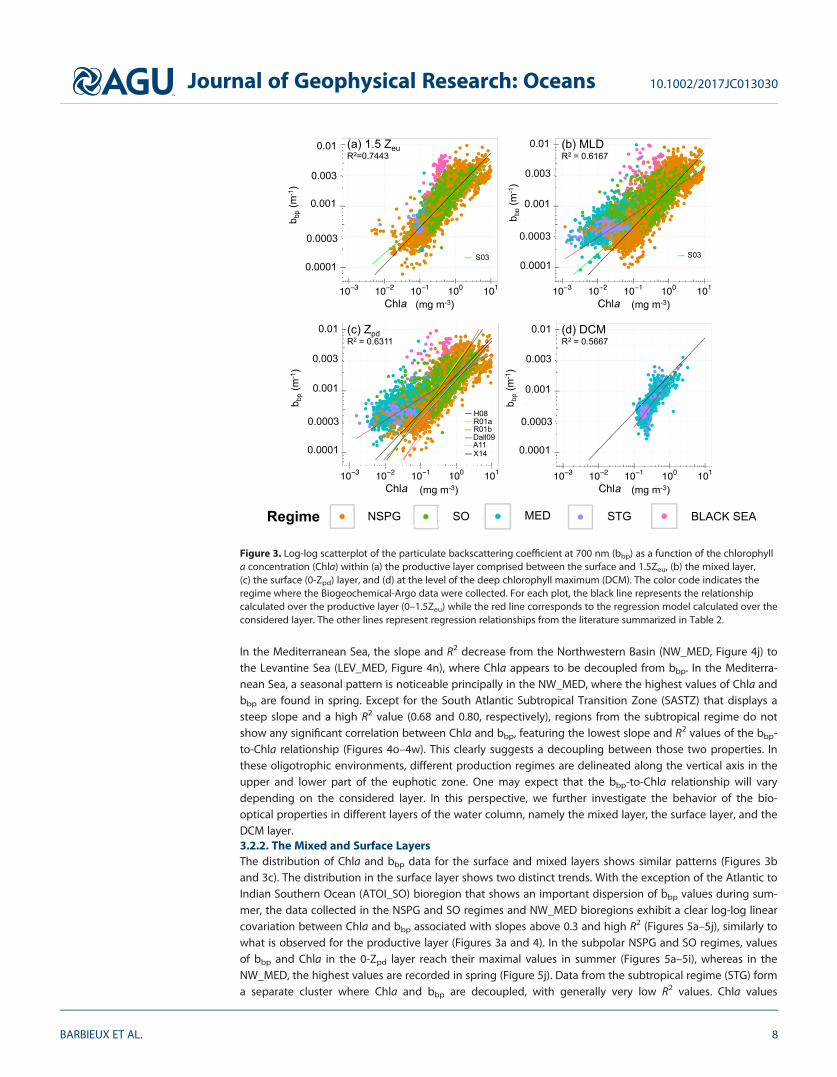
In the Mediterranean Sea, the slope and R2 decrease from the Northwestern Basin (NW_MED, Figure 4j) tothe Levantine Sea (LEV_MED, Figure 4n), where Chla appears to be decoupled from bbp. In the Mediterra-nean Sea, a seasonal pattern is noticeable principally in the NW_MED, where the highest values of Chla andbbp are found in spring. Except for the South Atlantic Subtropical Transition Zone (SASTZ) that displays asteep slope and a high R2 value (0.68 and 0.80, respectively), regions from the subtropical regime do notshow any significant correlation between Chla and bbp, featuring the lowest slope and R2 values of the bbp-to-Chla relationship (Figures 4o–4w). This clearly suggests a decoupling between those two properties. Inthese oligotrophic environments, different production regimes are delineated along the vertical axis in theupper and lower part of the euphotic zone. One may expect that the bbp-to-Chla relationship will varydepending on the considered layer. In this perspective, we further investigate the behavior of the bio-optical properties in different layers of the water column, namely the mixed layer, the surface layer, and theDCM layer.3.2.2. The Mixed and Surface LayersThe distribution of Chla and bbp data for the surface and mixed layers shows similar patterns (Figures 3band 3c). The distribution in the surface layer shows two distinct trends. With the exception of the Atlantic toIndian Southern Ocean (ATOI_SO) bioregion that shows an important dispersion of bbp values during sum-mer, the data collected in the NSPG and SO regimes and NW_MED bioregions exhibit a clear log-log linearcovariation between Chla and bbp associated with slopes above 0.3 and high R2 (Figures 5a–5j), similarly towhat is observed for the productive layer (Figures 3a and 4). In the subpolar NSPG and SO regimes, valuesof bbp and Chla in the 0-Zpd layer reach their maximal values in summer (Figures 5a–5i), whereas in theNW_MED, the highest values are recorded in spring (Figure 5j). Data from the subtropical regime (STG) forma separate cluster where Chla and bbp are decoupled, with generally very low R2 values. Chla values

Figure 3. Log-log scatterplot of the particulate backscattering coefficient at 700 nm (bbp) as a function of the chlorophylla concentration (Chla) within (a) the productive layer comprised between the surface and 1.5Zeu, (b) the mixed layer,(c) the surface (0-Zpd) layer, and (d) at the level of the deep chlorophyll maximum (DCM). The color code indicates theregime where the Biogeochemical-Argo data were collected. For each plot, the black line represents the relationshipcalculated over the productive layer (0–1.5Zeu) while the red line corresponds to the regression model calculated over theconsidered layer. The other lines represent regression relationships from the literature summarized in Table 2.

Journal of Geophysical Research: Oceans 10.1002/2017JC013030

BARBIEUX ET AL. 8

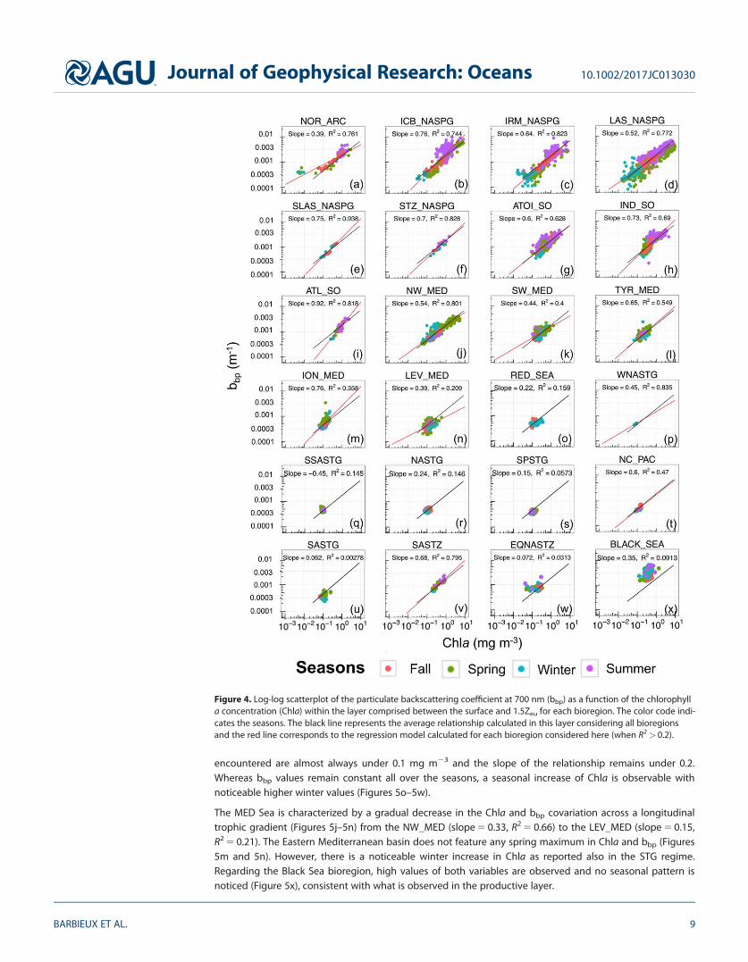
encountered are almost always under 0.1 mg m23 and the slope of the relationship remains under 0.2.Whereas bbp values remain constant all over the seasons, a seasonal increase of Chla is observable withnoticeable higher winter values (Figures 5o–5w).

The MED Sea is characterized by a gradual decrease in the Chla and bbp covariation across a longitudinaltrophic gradient (Figures 5j–5n) from the NW_MED (slope 5 0.33, R2 5 0.66) to the LEV_MED (slope 5 0.15,R2 5 0.21). The Eastern Mediterranean basin does not feature any spring maximum in Chla and bbp (Figures5m and 5n). However, there is a noticeable winter increase in Chla as reported also in the STG regime.Regarding the Black Sea bioregion, high values of both variables are observed and no seasonal pattern isnoticed (Figure 5x), consistent with what is observed in the productive layer.

Figure 4. Log-log scatterplot of the particulate backscattering coefficient at 700 nm (bbp) as a function of the chlorophylla concentration (Chla) within the layer comprised between the surface and 1.5Zeu for each bioregion. The color code indi-cates the seasons. The black line represents the average relationship calculated in this layer considering all bioregionsand the red line corresponds to the regression model calculated for each bioregion considered here (when R2> 0.2).

Journal of Geophysical Research: Oceans 10.1002/2017JC013030

BARBIEUX ET AL. 9

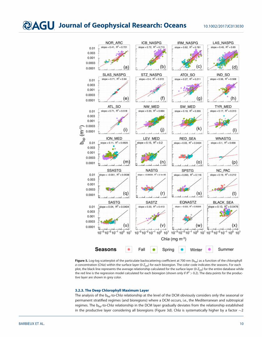
3.2.3. The Deep Chlorophyll Maximum LayerThe analysis of the bbp-to-Chla relationship at the level of the DCM obviously considers only the seasonal orpermanent stratified regimes (and bioregions) where a DCM occurs, i.e., the Mediterranean and subtropicalregimes. The bbp-to-Chla relationship in the DCM layer gradually deviates from the relationship establishedin the productive layer considering all bioregions (Figure 3d). Chla is systematically higher by a factor �2

Figure 5. Log-log scatterplot of the particulate backscattering coefficient at 700 nm (bbp) as a function of the chlorophylla concentration (Chla) within the surface layer (0-Zpd) for each bioregion. The color code indicates the seasons. For eachplot, the black line represents the average relationship calculated for the surface layer (0-Zpd) for the entire database whilethe red line is the regression model calculated for each bioregion (shown only if R2> 0.2). The data points for the produc-tive layer are shown in grey color.

Journal of Geophysical Research: Oceans 10.1002/2017JC013030

BARBIEUX ET AL. 10

regardless of the bioregion and never reaches values below 0.1 mg m23 (Figures 3d and B1 in electronicsupporting information B).

The subset of data from this layer also shows two distinct trends in the bbp-to-Chla relationship, for Chla val-ues below or above 0.3 mg m23 (Figure 3d). For Chla> 0.3 mg m23, a positive correlation between bbp andChla can be noticed, although with a large dispersion of the data around the regression line, whereas forChla< 0.3 mg m23, Chla and bbp exhibit a strong decoupling. The MED Sea (Figures B1a–B1e in electronicsupporting information B) is characterized by a stronger covariation between Chla and bbp than the STGregime (Figures B1f–B1n in electronic supporting information B) (R2 5 0.53 for NW_MED versus R2 5 0.10 forSPSTG). In the Mediterranean Sea, DCMs are seasonal phenomena occurring essentially in summer or fall(e.g., Siokou-Frangou et al., 2010). A covariation between bbp and Chla occurs as soon as a DCM takes place,with maximum values of bbp and Chla encountered in summer when the DCM is the most pronounced, inboth the western and eastern Mediterranean basins. On the opposite, in the STG regime where durablestratification takes place, DCMs appear as a permanent pattern. The bbp and Chla variations are decoupledand the highest values of both variables are recorded in spring or fall.

4. Discussion

The present analysis of a global BGC-Argo database indicates a general power relationship between bbp

and Chla in the productive layer as well as in the surface and mixed layers. Nevertheless, the analysis of sub-sets of data suggests a large second-order variability around the global mean relationships, depending onthe considered range of values in Chla and bbp, layer of the water column, region, or season. In this section,we investigate the sources of variability around the average bbp-to-Chla relationship in our database.

4.1. General Relationship Between Chla and bbp

The chlorophyll a concentration is the most commonly used proxy for the phytoplankton carbon biomass(Cullen, 1982; Siegel et al., 2013), whereas the particulate backscattering coefficient is considered as a proxyof the POC in open ocean (Balch et al., 2001; Cetinic et al., 2012; Dall’Olmo & Mork, 2014; Stramski et al.,1999) and provides information on the whole pool of particles, not specifically on phototrophic organisms.Over broad biomass gradients, the stock of POC covaries with phytoplankton biomass and hence bbp andChla show substantial covariation. This is what is observed in the present study when the full database isconsidered (Figure 3a). This is also the case when we examine subsets of data from the NSPG and SOregimes that feature strong seasonality and show relatively constant relationships between bbp and Chla(Figures 3a–3c, 4a–4I, and 5a–5i). In such environments, an increase in the concentration of chlorophyll a isassociated with an increase in bbp. Such significant relationships between bbp and Chla have indeed beenreported in several studies based on relatively large data sets (Huot et al., 2008) or measurements fromseasonally dynamic systems (Antoine et al., 2011; Stramska et al., 2003; Xing et al., 2014). Our resultscorroborate these studies and yield a global relationship of the form bbp(700) 5 0.00181 (60.000001)Chla0.605 (60.005) for the productive layer.

Nevertheless, the bbp-to-Chla relationship is largely variable depending on the considered layer of the watercolumn. Regarding the mixed and surface layers, our study suggests a general relationship with determina-tion coefficients smaller than those calculated for the productive layer. The intercept (�0.0017) and moreimportantly the slope values (�0.36) associated with the surface layer are also lower than those associatedwith the productive layer (Table 3); hence, for a given level of bbp, the Chla is lower for the surface layerthan predicted by the productive layer relationship. Empirical relationships of the literature previouslyestablished in various regions in the first few meters of the water column (Antoine et al., 2011; Dall’Olmoet al., 2009; Reynolds et al., 2001; Xing et al., 2014) always show steeper slope compared to our results forthe surface layer (Table 2).

To our knowledge, the present study proposes the first analysis of the bbp-to-Chla relationship within theDCM layer. A significant relationship between bbp and Chla is observed and it is associated with the steep-est slope, the highest RMSE and the lowest coefficient of determination in comparison with the other layers(Table 3). Thus, for the DCM layer, a given level of bbp is associated with higher values of Chla than pre-dicted by the global relationship of the productive layer.

Journal of Geophysical Research: Oceans 10.1002/2017JC013030

BARBIEUX ET AL. 11

In the next two sections, we will investigate the underlying processes leading to the existence or not of arelationship between bbp and Chla and explore the variability of this relationship along the vertical dimen-sion, the seasons and the distinct bioregions of the different regimes. For this purpose, we will consider thebehavior of the bbp:Chla ratio with respect to light conditions and phytoplankton community composition.

4.2. Influence of the Nature of the Particulate Assemblage on the bbp-to-Chla RelationshipAlthough the relationship between POC and bbp is evident in some regions, the particulate backscatteringcoefficient is not a direct proxy of POC. It depends on several parameters such as the concentration of par-ticles in the water column, their size distribution, shape, structure, and refractive index (Babin & Morel,2003; Huot et al., 2007; Morel & Bricaud, 1986; Whitmire et al., 2010). The bbp coefficient has been shown tobe very sensitive to the presence of picophytoplankton as well as of nonalgal particles of the submicronsize range (e.g., detritus, bacteria, and viruses), especially in oligotrophic waters (Ahn et al., 1992; Stramskiet al., 2001; Vaillancourt et al., 2004), but also to particles up to 10 mm (Loisel et al., 2007).

In regions with substantial inputs of mineral particles, a shift toward enhanced bbp values for a constantChla level occurs (Figures 4w and 4x, 5w and 5x). Substantial concentrations of mineral particles, submi-crometer particles of Saharan origin, for example, have been shown to cause significant increases in the par-ticulate backscattering signal (Claustre et al., 2002; Loisel et al., 2011; Prospero, 1996; Stramski et al., 2004).The EQNASTZ bioregion exhibits, for example, particularly high bbp values compared to the low Chla foundin the surface layer (Figures 4w and 5w). This is not surprising considering that this region is located in theEquatorial North Atlantic dust belt (Kaufman et al., 2005). The Black Sea is also characterized by a higher bbp

signal than predicted from Chla based on our global model (Figures 4x and 5x). This could be explained bythe fact that this enclosed sea follows a coastal trophic regime and is strongly influenced by river runoffthat may carry small and highly refractive lithogenic particles (Ludwig et al., 2009; Tanhua et al., 2013). Suchan increase in backscattering signal may also be related to coccolithophorid blooms (Balch et al., 1996a).These small calcifying microalgae highly backscatter light due to their calcium carbonate shell and theirpresence could explain the episodically higher bbp than predicted by the global regression model

Table 2Empirical Relationship Between the Particulate Backscattering Coefficient (bbp) and the Concentration Of Chlorophyll a (Chl a) Previously Published in the LiteratureWith the Corresponding Reference and Abbreviation, Region, and Layer of the Water Column Considered for Analysis

Empirical relationship RegionLayer in the

water column Abbreviation Reference

bbp(k) 5 0.0023 – 0.000005(k – 550) Chla0.565 1 0.000486(k–550)

Eastern South Pacific 2/Kd(490) H08 Huot et al. (2008)

bbp(555) 5 0.004 Chla0.822 Antarctic Polar Front 15 m R0l a Reynolds et al. (2001)bbp(555) 5 0.001 Chla0.667 Ross Sea 15 m R0l b Reynolds et al. (2001)bbp(555) 5 0.0019 Chla0.61 Polar North Atlantic MLD S03 Stramska et al. (2003)bbp(526) 5 0.00386 Chla Eastern Equatorial Pacific Surface Dall09 Dall’Olmo et al. (2009) modified

in Xing et al. (2014)bbp(532) 5 0.003 Chla0.786 North Atlantic Subpolar Gyre Zpd X14 Xing et al. (2014)bbp(555) 5 0.00197 Chla0.647 North-Western Mediterranean

Sea and Santa Barbara ChannelSurface All Antoine et al. (2011)

Table 3Empirical Relationship Obtained Between the Particulate Backscattering Coefficient (bbp) and the Concentration ofChlorophyll a (Chl a) for the Different Layers of the Water Column Considered in This Study

Empirical relationship Water column layer R2 RMSE Number of data

bbp(700) 5 0.00174 Chla0.360 0-Zpd 0.6311 0.000942 5,253bbp(700) 5 0.00171 Chla0.373 0-MLD 0.6167 0.000932 8,743bbp(700) 5 0.00147 Chla0.753 DCM 0.5667 0.00104 1,628bbp(700) 5 0.00181 Chla0.605 021.5Zeu 0.7443 0.000967 5,250

Note. We also indicate the associated statistics: Root-mean-squared error (RMSE) and coefficient of determination R2

for the significance level of p< 0.001.

Journal of Geophysical Research: Oceans 10.1002/2017JC013030

BARBIEUX ET AL. 12

particularly in the Black Sea where coccolithophorid blooms are frequently reported (Cokacar et al., 2001;Kopelevich et al., 2014) or in the Iceland Basin (Balch et al., 1996b; Holligan et al., 1993; Figure 4b or 5b).

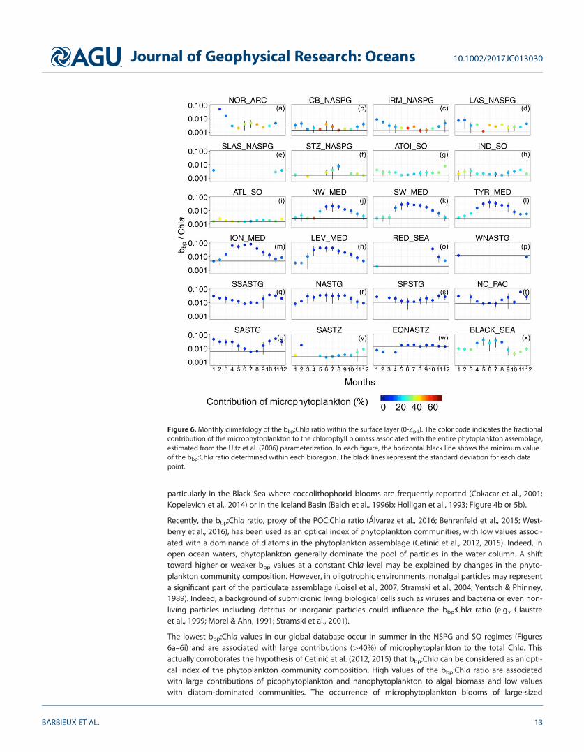
Recently, the bbp:Chla ratio, proxy of the POC:Chla ratio (�Alvarez et al., 2016; Behrenfeld et al., 2015; West-berry et al., 2016), has been used as an optical index of phytoplankton communities, with low values associ-ated with a dominance of diatoms in the phytoplankton assemblage (Cetinic et al., 2012, 2015). Indeed, inopen ocean waters, phytoplankton generally dominate the pool of particles in the water column. A shifttoward higher or weaker bbp values at a constant Chla level may be explained by changes in the phyto-plankton community composition. However, in oligotrophic environments, nonalgal particles may representa significant part of the particulate assemblage (Loisel et al., 2007; Stramski et al., 2004; Yentsch & Phinney,1989). Indeed, a background of submicronic living biological cells such as viruses and bacteria or even non-living particles including detritus or inorganic particles could influence the bbp:Chla ratio (e.g., Claustreet al., 1999; Morel & Ahn, 1991; Stramski et al., 2001).

The lowest bbp:Chla values in our global database occur in summer in the NSPG and SO regimes (Figures6a–6i) and are associated with large contributions (>40%) of microphytoplankton to the total Chla. Thisactually corroborates the hypothesis of Cetinic et al. (2012, 2015) that bbp:Chla can be considered as an opti-cal index of the phytoplankton community composition. High values of the bbp:Chla ratio are associatedwith large contributions of picophytoplankton and nanophytoplankton to algal biomass and low valueswith diatom-dominated communities. The occurrence of microphytoplankton blooms of large-sized

Figure 6. Monthly climatology of the bbp:Chla ratio within the surface layer (0-Zpd). The color code indicates the fractionalcontribution of the microphytoplankton to the chlorophyll biomass associated with the entire phytoplankton assemblage,estimated from the Uitz et al. (2006) parameterization. In each figure, the horizontal black line shows the minimum valueof the bbp:Chla ratio determined within each bioregion. The black lines represent the standard deviation for each datapoint.

Journal of Geophysical Research: Oceans 10.1002/2017JC013030

BARBIEUX ET AL. 13

phytoplankton community is indeed well known in the NSPG regime (Barton et al., 2015; Cetinic et al., 2015;Li, 2002) or in some productive regions of the Southern Ocean (Georges et al., 2014; Mendes et al., 2015;Uitz et al., 2009). Similarly, in the NW_MED bioregion, low bbp:Chla values are accompanied by large contri-butions of microphytoplankton during the spring bloom (Marty & Chiav�erini, 2010; Mayot et al., 2016;Siokou-Frangou et al., 2010). On the opposite, high bbp:Chla values in summer are rather associated withdominant contributions of the picophytoplankton and nanophytoplankton to the total chlorophyll biomass(Figure 6j) and also possibly to a higher proportion of nonalgal particles, consistently with Navarro et al.(2014) or Sammartino et al. (2015).

In the rest of the Mediterranean Basin (SW_MED, TYR_MED and the Eastern Basin) (Figures 6k–6n) as well asin the subtropical regime, the phytoplankton biomass is essentially constant throughout the year with highbbp:Chla values in summer, lower values in winter, and a relatively constant picoplankton-dominated algalcommunity (Figures 6o–6w; Dandonneau et al., 2004; Ras et al., 2008; Uitz et al., 2006). In this region, theseasonal cycle of the bbp:Chla ratio does not seem to be influenced at a first order by changes in phyto-plankton community composition.

4.3. Influence of Photoacclimation on the bbp-to-Chla RelationshipThe Chla is an imperfect proxy of phytoplankton biomass that varies not only with phytoplankton carbonbiomass but also with environmental conditions such as light, temperature, or nutrient availability (Babinet al., 1996; Cleveland et al., 1989; Geider et al., 1997). Phytoplankton cells adjust their intracellular Chla inresponse to changes in light conditions through the process of photoacclimation (Dubinsky & Stambler,2009; Eisner et al., 2003; Falkowski & Laroche, 1991; Lindley et al., 1995). Photoacclimation-induced varia-tions in intracellular Chla may cause large changes in the Chla-to-carbon ratio (Behrenfeld et al., 2005;Geider, 1987; Sathyendranath et al., 2009) and, thus, changes in the bbp-to-Chla ratio (Behrenfeld & Boss,2003; Siegel et al., 2005). In the upper oceanic layer of the water column, photoacclimation to high lightmay result in an increase in the bbp-to-Chla ratio whereas a decrease in this ratio occurs in DCM layers or inthe upper layer during winter time in subpolar regimes (NSPG and SO) where photoacclimation to low lightoccurs.

The impact of light conditions on the bbp:Chla ratio in the different regimes is illustrated in Figure 7. Signifi-cant trends are observed in the different layers of the water column for all regimes except for the Black Sea.In the NSPG and SO regimes, the bbp:Chla ratio remains relatively constant with respect to the normalizedPAR regardless of the considered layer of the water column (Figures 7a–7c). In contrast, the MediterraneanSea and the subtropical gyres show a decoupling between bbp and Chla (Figures 5k–5w) so the bbp:Chlaratio in the productive, mixed or surface layer increases with an increase in the normalized PAR (Figures 7a–7c). The seasonal cycle of the bbp:Chla ratio in these regimes results from variations in Chla whereas bbp

remains relatively constant over the seasons (not shown). Thus, our results suggest that the variability in thebbp:Chla ratio in the NSPG and SO regimes is not driven at first order by phytoplankton acclimation to lightlevel even if such a process is known to occur at shorter temporal and spatial scales in those regimes (Beh-renfeld et al., 2015; Lutz et al., 2003). On the opposite, in both the MED and STG regimes the bbp:Chla ratiovariations are essentially driven by phytoplankton photoacclimation.

In these oligotrophic regimes, Chla within the DCM layer is at least a factor of 2 higher than in the produc-tive layer (Figure 6). In the lower part of the euphotic zone, phytoplankton cells hence adjust their intracellu-lar Chla to low light conditions, resulting in a decrease in the bbp:Chla ratio. In addition, the bbp:Chla ratio inthis layer seems to remain constant within a regime regardless of absolute light conditions (Figure 7d).Actually, the absolute values of PAR essentially vary between 10 and 25 mmol quanta m22 s21 in all the bio-regions along the year with values exceeding 50 mmol quanta m22 s21 only in the NW_MED and EQNASTZbioregions. As reported by Letelier et al. (2004) and Mignot et al. (2014), the DCM may follow a given iso-lume along the seasonal cycle and is thus essentially light driven. Finally, we suggest that the relative homo-geneity of both the environmental (PAR) conditions and phytoplankton community composition at theDCM level in subtropical regimes may explain the relative stability of the bbp:Chla values in this water col-umn layer. In the Mediterranean Sea, in contrast, some studies evoke changes in phytoplankton communi-ties in the DCM layer (Crombet et al., 2011) suggesting our results might be further explored when relevantdata are available.

Journal of Geophysical Research: Oceans 10.1002/2017JC013030

BARBIEUX ET AL. 14

4.4. Variability in the bbp-to-Chla Relationship Is Driven by a Combination of FactorsIn the previous sections, we examined the processes that potentially drive the variability in the bbp-to-Chlarelationship in the various oceanic regimes considered here.

In the subpolar regimes NSPG and SO, changes in the composition of the particle assemblage, phytoplank-ton communities in particular, are likely the first-order driver of the seasonal variability in the bbp-to-Chlaratio (Figure 8). In these regimes, the bbp:Chla ratio remains constant regardless of the light intensity inboth the productive and surface layers suggesting that phytoplankton photoacclimation is likely not animportant driver of the variability in the bbp-to-Chla relationship. We note, however, that in the SO otherfactors may come into play, such as the light-mixing regime or iron limitation (e.g., Blain et al., 2007, 2013;Boyd, 2002). On the opposite, in the subtropical regime, Chla and bbp are decoupled in the surface layer aswell as in the DCM layer. Thus, photoacclimation seems to be the main process driving the vertical and sea-sonal variability of the bbp-to-Chla relationship, although a varying contribution of nonalgal particles to theparticle pool cannot be excluded.

Whereas the subpolar and the subtropical regimes behave as a ‘‘biomass regime’’ and a ‘‘photoacclimationregime’’ (sensu Siegel et al., 2005), respectively, the Mediterranean Sea stands as an intermediate regimebetween these two end-members. The large number of data available in the Mediterranean allows us todescribe this intermediate situation (Figure 8). The Mediterranean Sea appears as a more complex and vari-able system than the stable and resilient subtropical gyres. Along with the ongoing development of theglobal BGC-Argo program and associated float deployments, additional data collected in underrepresentedregions will become available to make our database more robust and will help to improve our analysis. Inthe surface layer of the Mediterranean system, a high bbp:Chla ratio in summer might be attributed not onlyto (i) a background of submicronic living biological cells such as viruses and bacteria or large contributionof nonliving particles including detritus or inorganic particles (Bricaud et al., 2004; Claustre et al., 1999;

Figure 7. Histogram of the monthly median bbp:Chla ratio as a function of the normalized Photosynthetically AvailableRadiation (PARnorm) for each regime within (a) the layer comprised between the surface and 1.5Zeu, (b) the mixed layer,(c) the surface layer, and (d) within the DCM layer. The color code indicates the regimes in which the BGC-Argo data werecollected. Note the different y scale for Figure 7d compared to Figures 7a–7c. The black lines on the top of each bar repre-sent the standard deviation.

Journal of Geophysical Research: Oceans 10.1002/2017JC013030

BARBIEUX ET AL. 15

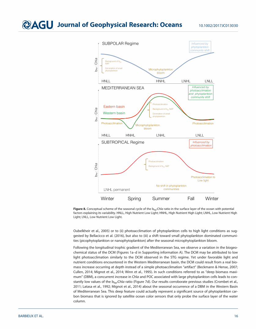
Oubelkheir et al., 2005) or to (ii) photoacclimation of phytoplankton cells to high light conditions as sug-gested by Bellacicco et al. (2016), but also to (iii) a shift toward small phytoplankton dominated communi-ties (picophytoplankton or nanophytoplankton) after the seasonal microphytoplankton bloom.

Following the longitudinal trophic gradient of the Mediterranean Sea, we observe a variation in the biogeo-chemical status of the DCM (Figures 1a–d in Supporting information A). The DCM may be attributed to lowlight photoacclimation similarly to the DCM observed in the STG regime. Yet under favorable light andnutrient conditions encountered in the Western Mediterranean basin, the DCM could result from a real bio-mass increase occurring at depth instead of a simple photoacclimation ‘‘artifact’’ (Beckmann & Hense, 2007;Cullen, 2014; Mignot et al., 2014; Winn et al., 1995). In such conditions referred to as ‘‘deep biomass maxi-mum’’ (DBM), a concurrent increase in Chla and POC associated with large phytoplankton cells leads to con-stantly low values of the bbp:Chla ratio (Figure 7d). Our results corroborate previous studies (Crombet et al.,2011; Latasa et al., 1992; Mignot et al., 2014) about the seasonal occurrence of a DBM in the Western Basinof Mediterranean Sea. This deep feature could actually represent a significant source of phytoplankton car-bon biomass that is ignored by satellite ocean color sensors that only probe the surface layer of the watercolumn.

Figure 8. Conceptual scheme of the seasonal cycle of the bbp:Chla ratio in the surface layer of the ocean with potentialfactors explaining its variability. HNLL, High Nutrient Low Light; HNHL, High Nutrient High Light; LNHL, Low Nutrient HighLight; LNLL, Low Nutrient Low Light.

Journal of Geophysical Research: Oceans 10.1002/2017JC013030

BARBIEUX ET AL. 16

5. Conclusions

The main goal of the present study was to examine the variability of the relationship between the particu-late backscattering coefficient and the chlorophyll a concentration over a broad range of oceanic condi-tions. Using an extensive BGC-Argo profiling float database, we investigated the sources of variability in thisrelationship with respect to the vertical dimension as well as on a seasonal and regional scale. In accordancewith previous studies (Antoine et al., 2011; Dall’Olmo et al., 2009; Huot et al., 2008; Reynolds et al., 2001;Stramska et al., 2003; Xing et al., 2014) and consistently with the so-called ‘‘bio-optical assumption’’ (Siegelet al., 2005; Smith & Baker, 1978b), a general covariation between bbp and Chla is observed at a global scalein the productive layer of the water column (0–1.5Zeu). Although this covariation seems to be permanent insubpolar regimes in relation with large-amplitude phytoplankton biomass seasonal cycles (Boss & Behren-feld, 2010; Henson et al., 2006; Lacour et al., 2015), several nuances have been revealed according to theseason, considered layer of the water column and bioregion. We suggest that the bbp:Chla ratio, proxy ofthe C:Chla ratio (Behrenfeld et al., 2015; Westberry et al., 2016), can be used either as an index of the nature(composition and size) of the particle assemblage in a ‘‘biomass regime’’ (NSPG and SO regimes and West-ern Mediterranean basin) or as a photophysiological index in a ‘‘photoacclimation regime’’ (STG regime andEastern Mediterranean basin).

The present analysis provides insights into the coupling between major proxies of the POC and phytoplank-ton biomass in key regimes encountered in the world’s open oceans. It points to the strong potential of therecently available global BGC-Argo float database to address regional or seasonal nuances in first-order rela-tionships that have been established in the past on admittedly restricted data sets. In addition, this studystresses out the large variability in the bbp-to-Chla relationship, which is critical to the bio-optical modelingof the bbp coefficient in several semiempirical ocean color models (Garver & Siegel, 1997; Lee et al., 2002;Maritorena et al., 2002). Indeed, bio-optical and reflectance models require detailed knowledge and param-eterization of the average trends in the inherent optical properties, especially in open ocean waters wherethese trends can be related to Chla. Although the analysis of the impact of such variability on ocean colormodeling is out of the scope of the present paper, we expect our analysis to be potentially useful in thecontext of applications to ocean color. Finally, as the amount of BGC-float data will continue to increase, itwill be possible to reassess the variability of bio-optical relationships and to establish new ‘‘global’’ stand-ards and regional parameterizations.

ReferencesAhn, Y.-H., Bricaud, A., & Morel, A. (1992). Light backscattering efficiency and related properties of some phytoplankters. Deep Sea Research

Part A. Oceanographic Research Papers, 39(11–12), 1835–1855.�Alvarez, E., Mor�an, X. A. G., L�opez-Urrutia, �A., & Nogueira, E. (2016). Size-dependent photoacclimation of the phytoplankton community in

temperate shelf waters (southern Bay of Biscay). Marine Ecology Progress Series, 543, 73–87. https://doi.org/10.3354/meps11580Antoine, D., Siegel, D. A., Kostadinov, T., Maritorena, S., Nelson, N. B., Gentili, B., . . . Guillocheau, N. (2011). Variability in optical particle back-

scattering in contrasting bio-optical oceanic regimes. Limnology and Oceanography, 56(3), 955–973. https://doi.org/10.4319/lo.2011.56.3.0955

Babin, M., Morel, A., Fournier-Sicre, V., & Fell, F. (2003). Light scattering properties of marine particles in coastal and open ocean waters asrelated to the particle mass concentration. Limnology and Oceanography, 48(2), 843–859. https://doi.org/10.4319/lo.2003.48.2.0843

Babin, M., Morel, A., & Gentili, B. (1996). Remote sensing of sea surface Sun-induced chlorophyll fluorescence: Consequences of natural var-iations in the optical characteristics of phytoplankton and the quantum yield of chlorophyll a fluorescence. International Journal ofRemote Sensing, 17(12), 2417–2448.

Balch, W. M., Drapeau, D. T., Fritz, J. J., Bowler, B. C., & Nolan, J. (2001). Optical backscattering in the Arabian Sea—Continuous underwaymeasurements of particulate inorganic and organic carbon. Deep Sea Research Part I: Oceanographic Research Papers, 48(11), 2423–2452. https://doi.org/10.1016/S0967-0637(01)00025-5

Balch, W. M., Kilpatrick, K. A., Holligan, P., Harbour, D., & Fernandez, E. (1996a). The 1991 coccolithophore bloom in the central North Atlan-tic. 2. Relating optics to coccolith concentration. Limnology and Oceanography, 41(8), 1684–1696. https://doi.org/10.4319/lo.1996.41.8.1684

Balch, W. M., Kilpatrick, K. A., & Trees, C. C. (1996b). The 1991 coccolithorphore bloom in the central North Atlantic: I. Optical properties andfactors affecting their distribution. Limnology and Oceanography, 41(8), 1669–1683.

Barbieux, M., Organelli, E., Claustre, H., Schmechtig, C., Poteau, A., Boss, E., . . . Xing, X. (2017). A global database of vertical profiles derivedfrom Biogeochemical Argo float measurements for biogeochemical and bio-optical applications. SEANOE. https://doi.org/10.17882/49388

Barton, A. D., Lozier, M. S., & Williams, R. G. (2015). Physical controls of variability in North Atlantic phytoplankton communities. Limnologyand Oceanography, 60(1), 181–197. https://doi.org/10.1002/lno.10011

Beckmann, A., & Hense, I. (2007). Beneath the surface: Characteristics of oceanic ecosystems under weak mixing conditions—A theoreticalinvestigation. Progress in Oceanography, 75(4), 771–796. https://doi.org/10.1016/j.pocean.2007.09.002

Behrenfeld, M. J., & Boss, E. (2003). The beam attenuation to chlorophyll ratio: An optical index of phytoplankton physiology in the surfaceocean? Deep Sea Research Part I: Oceanographic Research Papers, 50(12), 1537–1549. https://doi.org/10.1016/j.dsr.2003.09.002

AcknowledgmentsThis paper represents a contribution tothe following research projects:remOcean (funded by the EuropeanResearch Council, grant 246777), NAOS(funded by the Agence Nationale de laRecherche in the frame of the French‘‘Equipement d’avenir’’ program, grantANR J11R107-F), the SOCLIM (SouthernOcean and climate) project supportedby the French research program LEFE-CYBER of INSU-CNRS, the ClimateInitiative of the foundation BNP Paribasand the French polar institute (IPEV),AtlantOS (funded by the EuropeanUnion’s Horizon 2020 Research andInnovation program, grant 2014–633211), E-AIMS (funded by theEuropean Commission’s FP7 project,grant 312642), U.K. Bio-Argo (funded bythe British Natural EnvironmentResearch Council—NERC, grant NE/L012855/1), REOPTIMIZE (funded by theEuropean Union’s Horizon 2020Research and Innovation program,Marie Skłodowska-Curie grant 706781),Argo-Italy (funded by the Italian Ministryof Education, University and Research -MIUR), and the French Bio-Argoprogram (BGC-Argo France; funded byCNES-TOSCA, LEFE Cyber, and GMMC).We thank the PIs of several BGC-Argofloats missions and projects: GiorgioDall’Olmo (Plymouth Marine Laboratory,United Kingdom; E-AIMS and U.K. Bio-Argo); Kjell-Arne Mork (Institute ofMarine Research, Norway; E-AIMS);Violeta Slabakova (Bulgarian Academyof Sciences, Bulgaria; E-AIMS); EmilStanev (University of Oldenburg,Germany; E-AIMS); Claire Lo Monaco(Laboratoire d’Oc�eanographie et duClimat: Exp�erimentations et ApprochesNum�eriques); Pierre-Marie Poulain(National Institute of Oceanography andExperimental Geophysics, Italy; Argo-Italy); Sabrina Speich (Laboratoire deM�et�eorologie Dynamique, France; LEFE-GMMC); Virginie Thierry (Ifremer, France;LEFE-GMMC); Pascal Conan(Observatoire Oc�eanologique deBanyuls sur mer, France; LEFE-GMMC);Laurent Coppola (Laboratoired’Oc�eanographie de Villefranche,France; LEFE-GMMC); Anne Petrenko(Mediterranean Institute ofOceanography, France; LEFE-GMMC);and Jean-Baptiste Sall�ee (Laboratoired’Oc�eanographie et du Climat, France;LEFE-GMMC). Collin Roesler (BowdoinCollege, USA) and Yannick Huot(University of Sherbrooke, Canada) areacknowledged for useful commentsand fruitful discussion. We also thankthe International Argo Program and theCORIOLIS project that contribute tomake the data freely and publiclyavailable. Data referring to Organelliet al. (2016a; https://doi.org/10.17882/47142) and Barbieux et al. (2017;https://doi.org/10.17882/49388) arefreely available on SEANOE.

Journal of Geophysical Research: Oceans 10.1002/2017JC013030

BARBIEUX ET AL. 17

Behrenfeld, M. J., Boss, E., Siegel, D. A., & Shea, D. M. (2005). Carbon-based ocean productivity and phytoplankton physiology from space.Global Biogeochemical Cycles, 19(1). https://doi.org/10.1029/2004GB002299

Behrenfeld, M. J., O’Malley, R. T., Boss, E. S., Westberry, T. K., Graff, J. R., Halsey, K. H., . . . Brown, M. B. (2015). Revaluating ocean warmingimpacts on global phytoplankton. Nature Climate Change, 6(3), 323–330. https://doi.org/10.1038/nclimate2838

Bellacicco, M., Volpe, G., Colella, S., Pitarch, J., & Santoleri, R. (2016). Role of photoacclimation on phytoplankton’s seasonal cycle in the Med-iterranean Sea through satellite ocean color data. Remote Sensing of Environment, 184, 595–604. https://doi.org/10.1016/j.rse.2016.08.004

Biogeochemical-Argo Planning Group. (2016). In H. Claustre & K. Johnson (Eds.), The scientific rationale, design, and implementation plan fora Biogeochemical-Argo float array (Report). https://doi.org/10.13155/46601

Birge, R. T. (1939). The propagation of errors. American Journal of Physics, 7(6), 351–357. https://doi.org/10.1119/1.1991484Bishop, J. K. B. (2009). Autonomous observations of the ocean biological carbon pump. Oceanography, 22(2), 182–193. https://doi.org/10.

5670/oceanog.2011.65Blain, S., Qu�eguiner, B., Armand, L., Belviso, S., Bombled, B., Bopp, L., . . . Wagener, T. (2007). Effect of natural iron fertilization on carbon

sequestration in the Southern Ocean. Nature, 446(7139), 1070–1074. https://doi.org/10.1038/nature05700Blain, S., Renaut, S., Xing, X., Claustre, H., & Guinet, C. (2013). Instrumented elephant seals reveal the seasonality in chlorophyll and light-

mixing regime in the iron-fertilized Southern Ocean. Geophysical Research Letters, 40(24), 6368–6372. https://doi.org/10.1002/2013GL058065

Boss, E., & Behrenfeld, M. (2010). In situ evaluation of the initiation of the North Atlantic phytoplankton bloom. Geophysical Research Letters,37, L18603. https://doi.org/10.1029/2010GL044174

Boss, E., & Pegau, W. S. (2001). Relationship of light scattering at an angle in the backward direction to the backscattering coefficient.Applied Optics, 40(30), 5503–5507. https://doi.org/10.1364/AO.40.005503

Boyd, P. W. (2002). Environmental factors controlling phytoplankton processes in the Southern Ocean. Journal of Phycology, 38(5), 844–861. https://doi.org/10.1046/j.1529-8817.2002.t01-1-01203.x

Brainerd, K. E., & Gregg, M. C. (1995). Surface mixed and mixing layer depths. Deep Sea Research Part I: Oceanographic Research Papers,42(9), 1521–1543.

Bricaud, A., Claustre, H., Ras, J., & Oubelkheir, K. (2004). Natural variability of phytoplanktonic absorption in oceanic waters: Influence of thesize structure of algal populations. Journal of Geophysical Research, 109(C11). https://doi.org/10.1029/2004JC002419

Bricaud, A., Roesler, C., & Zaneveld, J. R. V. (1995). In situ methods for measuring the inherent optical properties of ocean waters. Limnologyand Oceanography, 40(2), 393–410. https://doi.org/10.4319/lo.1995.40.2.0393

Briggs, N., Perry, M. J., Cetinic, I., Lee, C., D’Asaro, E., Gray, A. M., & Rehm, E. (2011). High-resolution observations of aggregate flux during asub-polar North Atlantic spring bloom. Deep Sea Research Part I: Oceanographic Research Papers, 58(10), 1031–1039. https://doi.org/10.1016/j.dsr.2011.07.007

Brown, C. A., Huot, Y., Werdell, P. J., Gentili, B., & Claustre, H. (2008). The origin and global distribution of second order variability in satelliteocean color and its potential applications to algorithm development. Remote Sensing of Environment, 112(12), 4186–4203. https://doi.org/10.1016/j.rse.2008.06.008

Cetinic, I., Perry, M. J., Briggs, N. T., Kallin, E., D’Asaro, E. A., & Lee, C. M. (2012). Particulate organic carbon and inherent optical propertiesduring 2008 North Atlantic Bloom Experiment. Journal of Geophysical Research, 117(C6). https://doi.org/10.1029/2011JC007771

Cetinic, I., Perry, M. J., D’Asaro, E., Briggs, N., Poulton, N., Sieracki, M. E., & Lee, C. M. (2015). A simple optical index shows spatial and tempo-ral heterogeneity in phytoplankton community composition during the 2008 North Atlantic Bloom Experiment. Biogeosciences, 12(7),2179–2194. https://doi.org/10.5194/bg-12-2179-2015

Claustre, H., Bishop, J., Boss, E., Bernard, S., Berthon, J.-F., Coatanoan, C., . . . Uitz, J. (2010). Bio-optical profiling floats as new observationaltools for biogeochemical and ecosystem studies: Potential synergies with ocean color remote sensing. Paper presented at Proceedings ofthe OceanObs’09: Sustained Ocean Observations and Information for Society Conference, ESA Publication WPP-306, Venice, Italy, Sep-tember 21–25. https://doi.org/10.5270/OceanObs09.cwp.17

Claustre, H., Morel, A., Babin, M., Cailliau, C., Marie, D., Marty, J.-C., . . . Vaulot, D. (1999). Variability in particle attenuation and chlorophyll fluo-rescence in the tropical Pacific: Scales, patterns, and biogeochemical implications. Journal of Geophysical Research, 104(C2), 3401–3422.

Claustre, H., Morel, A., Hooker, S. B., Babin, M., Antoine, D., Oubelkheir, K., . . . Maritorena, S. (2002). Is desert dust making oligotrophicwaters greener? Geophysical Research Letters, 29(10). https://doi.org/10.1029/2001GL014056

Cleveland, J. S., Perry, M. J., Kiefer, D. A., & Talbot, M. C. (1989). Maximal quantum yield of photosynthesis in the northwest Sargasso Sea.Journal of Marine Research, 47(4), 869–886.

Cokacar, T., Kubilay, N., & Oguz, T. (2001). Structure of Emiliania huxleyi blooms in the Black Sea surface waters as detected by SeaWIFSimagery. Geophysical Research Letters, 28(24), 4607–4610. https://doi.org/10.1029/2001GL013770

Crombet, Y., Leblanc, K., Queguiner, B., Moutin, T., Rimmelin, P., Ras, J., . . . Pujo-Pay, M. (2011). Deep silicon maxima in the stratified oligo-trophic Mediterranean Sea. Biogeosciences, 8(2), 459–475. https://doi.org/10.5194/bg-8-459-2011

Cullen, J. J. (1982). The deep chlorophyll maximum: Comparing vertical profiles of chlorophyll a. Canadian Journal of Fisheries and AquaticSciences, 39(5), 791–803.

Cullen, J. J. (2014). Subsurface chlorophyll maximum layers: Enduring enigma or mystery solved? Annual Review of Marine Science, 7, 207–239. https://doi.org/10.1146/annurev-marine-010213-135111

Dall’Olmo, G., & Mork, K. A. (2014). Carbon export by small particles in the Norwegian Sea. Geophysical Research Letters, 41(8), 2921–2927.https://doi.org/10.1002/2014GL059244

Dall’Olmo, G., Westberry, T. K., Behrenfeld, M. J., Boss, E., & Slade, W. H. (2009). Significant contribution of large particles to optical backscat-tering in the open ocean. Biogeosciences, 6(6), 947–967. https://doi.org/10.5194/bg-6-947-2009

Dandonneau, Y., Deschamps, P.-Y., Nicolas, J.-M., Loisel, H., Blanchot, J., Montel, Y., . . . B�ecu, G. (2004). Seasonal and interannual variabilityof ocean color and composition of phytoplankton communities in the North Atlantic, equatorial Pacific and South Pacific. Deep SeaResearch Part II: Topical Studies in Oceanography, 51(1–3), 303–318. https://doi.org/10.1016/j.dsr2.2003.07.018

de Boyer Mont�egut, C. (2004). Mixed layer depth over the global ocean: An examination of profile data and a profile-based climatology.Journal of Geophysical Research, 109(C12). https://doi.org/10.1029/2004JC002378

Dickey, T. D. (2003). Emerging ocean observations for interdisciplinary data assimilation systems. Journal of Marine Systems, 40–41, 5–48.https://doi.org/10.1016/S0924-7963(03)00011-3

Dubinsky, Z., & Stambler, N. (2009). Photoacclimation processes in phytoplankton: Mechanisms, consequences, and applications. AquaticMicrobial Ecology, 56(2–3), 163–176. https://doi.org/10.3354/ame01345

Journal of Geophysical Research: Oceans 10.1002/2017JC013030

BARBIEUX ET AL. 18

Eisner, L. B., Twardowski, M. S., Cowles, T. J., & Perry, M. J. (2003). Resolving phytoplankton photoprotective: Photosynthetic carotenoidratios on fine scales using in situ spectral absorption measurements. Limnology and Oceanography, 48(2), 632–646. https://doi.org/10.4319/lo.2003.48.2.0632

Falkowski, P. G., & Laroche, J. (1991). Acclimation to spectral irradiance in algae. Journal of Phycology, 27(1), 8–14. https://doi.org/10.1111/j.0022-3646.1991.00008.x

Flory, E. N., Hill, P. S., Milligan, T. G., & Grant, J. (2004). The relationship between floc area and backscatter during a spring phytoplanktonbloom. Deep Sea Research Part I: Oceanographic Research Papers, 51(2), 213–223. https://doi.org/10.1016/j.dsr.2003.09.012

Gardner, W. D., Mishonov, A. V., & Richardson, M. J. (2006). Global POC concentrations from in-situ and satellite data. Deep Sea ResearchPart II: Topical Studies in Oceanography, 53(5–7), 718–740. https://doi.org/10.1016/j.dsr2.2006.01.029

Garver, S. A., & Siegel, D. A. (1997). Inherent optical property inversion of ocean color spectra and its biogeochemical interpretation: 1.Time series from the Sargasso Sea. Journal of Geophysical Research, 102(C8), 607–625.

Geider, R. J. (1987). Light and temperature dependence of the carbon to chlorophyll a ratio in microalgae and cyanobacteria: Implicationsfor physiology and growth of phytoplankton. New Phytologist, 106(1), 1–34.

Geider, R. J. (1993). Quantitative phytoplankton physiology: Implications for primary production and phytoplankton growth. ICES MarineScience Symposium, 197, 52–62.

Geider, R. J., MacIntyre, H. L., & Kana, T. M. (1997). Dynamic model of phytoplankton growth and acclimation: Responses of the balancedgrowth rate and the chlorophyll a:carbon ratio to light, nutrient-limitation and temperature. Marine Ecology Progress Series, 148(1–3),187–200. https://doi.org/10.3354/meps148187

Georges, C., Monchy, S., Genitsaris, S., & Christaki, U. (2014). Protist community composition during early phytoplankton blooms in the nat-urally iron-fertilized Kerguelen area (Southern Ocean). Biogeosciences, 11(20), 5847–5863. https://doi.org/10.5194/bg-11-5847-2014

Gordon, H. R., & McCluney, W. R. (1975). Estimation of the depth of sunlight penetration in the sea for remote sensing. Applied Optics, 14(2),413–416. https://doi.org/10.1364/AO.14.000413

Gordon, R., Brown, O. B., Evans, H., Brown, W., Smith, C., Baker, K., & Clark, D. K. (1988). A semianalytic radiance model of ocean color. Jour-nal of Geophysical Research, 93(D9), 10909–10924.

Graff, J. R., Milligan, A. J., & Behrenfeld, M. J. (2012). The measurement of phytoplankton biomass using flow-cytometric sorting and ele-mental analysis of carbon. Limnology and Oceanography: Methods, 10(11), 910–920. https://doi.org/10.4319/lom.2012.10.910

Graff, J. R., Westberry, T. K., Milligan, A. J., Brown, M. B., Dall’Olmo, G., Van Dongen-Vogels, V., . . . Behrenfeld, M. J. (2015). Analytical phyto-plankton carbon measurements spanning diverse ecosystems. Deep Sea Research Part I: Oceanographic Research Papers, 102, 16–25.https://doi.org/10.1016/j.dsr.2015.04.006

Halsey, K. H., & Jones, B. M. (2015). Phytoplankton strategies for photosynthetic energy allocation. Annual Review of Marine Science, 7, 265–297. https://doi.org/10.1146/annurev-marine-010814-015813

Henson, S. A., Robinson, I., Allen, J. T., & Waniek, J. J. (2006). Effect of meteorological conditions on interannual variability in timing andmagnitude of the spring bloom in the Irminger Basin, North Atlantic. Deep Sea Research Part I: Oceanographic Research Papers, 53(10),1601–1615. https://doi.org/10.1016/j.dsr.2006.07.009

Holligan, P. M., Fern�andez, E., Aiken, J., Balch, W. M., Boyd, P., Burkill, P. H., . . . van der Wal, P. (1993). A biogeochemical study of the coccoli-thophore, Emiliania huxleyi, in the North Atlantic. Global Biogeochemical Cycles, 7(4), 879–900.

Honjo, S., Eglinton, T. I., Taylor, C. D., Ulmer, K. M., Sievert, S. M., Bracher, A., . . . Repeta, D. J. (2014). Understanding the role of the biologicalpump in the global carbon cycle: An imperative for ocean science. Oceanography, 27(3), 10–16. https://doi.org/10.5670/oceanog.2014.78

Huot, Y., & Antoine, D. (2016). Remote sensing reflectance anomalies in the ocean. Remote Sensing of Environment, 184, 101–111. https://doi.org/10.1016/j.rse.2016.06.002

Huot, Y., Babin, M., Bruyant, F., Grob, C., Twardowski, M. S., Claustre, H., & To, C. (2007). Relationship between photosynthetic parametersand different proxies of phytoplankton biomass in the subtropical ocean. Biogeosciences, 4(5), 853–868. https://doi.org/10.5194/bg-4-853-2007

Huot, Y., Morel, A., Twardowski, M. S., Stramski, D., & Reynolds, R. A. (2008). Particle optical backscattering along a chlorophyll gradient inthe upper layer of the eastern South Pacific Ocean. Biogeosciences, 5, 495–507. https://doi.org/10.5194/bg-5-495-2008

IOCCG. (2011). Bio-optical sensors on Argo floats. In H. Claustre (Ed.), Reports of the International Ocean-Colour Coordinating Group, No. 11.Dartmouth, Canada.

Johnson, K., & Claustre, H. (2016). Bringing Biogeochemistry into the Argo Age. Eos, Transactions American Geophysical Union, 1–7. https://doi.org/10.1029/2016EO062427

Kaufman, Y. J., Koren, I., Remer, L. A., Tanr�e, D., Ginoux, P., & Fan, S. (2005). Dust transport and deposition observed from the Terra-Moderate Resolution Imaging Spectroradiometer (MODIS) spacecraft over the Atlantic Ocean. Journal of Geophysical Research, 110(D10).https://doi.org/10.1029/2003JD004436

Kiefer, D. A., Diego, S., & Jolla, L. (1973). Chlorophyll a fluorescence in marine centric diatoms: Responses of chloroplasts to light and nutri-ent stress. Marine Biology, 23(1), 39–46.

Kopelevich, O., Burenkov, V., Sheberstov, S., Vazyulya, S., Kravchishina, M., Pautova, L., . . . Grigoriev, A. (2014). Satellite monitoring of cocco-lithophore blooms in the Black Sea from ocean color data. Remote Sensing of Environment, 146, 113–123. https://doi.org/10.1016/j.rse.2013.09.009

Ku, H. H. (1966). Notes on the use of propagation of error formulas. Journal of Research of the National Bureau of Standards, Section C: Engi-neering and Instrumentation, 70(4), 263. https://doi.org/10.6028/jres.070C.025

Lacour, L., Claustre, H., Prieur, L., & D’Ortenzio, F. (2015). Phytoplankton biomass cycles in the North Atlantic Subpolar Gyre: A similar mech-anism for two different blooms in the Labrador Sea. Geophysical Research Letters, 42, 5403–5410. https://doi.org/10.1002/2015GL064540

Latasa, M., Estrada, M., & Delgado, M. (1992). Plankton pigment relationships in the Northwestern Mediterranean during stratification.Marine Ecology Progress Series, 88, 61–73.

Lee, Z., Carder, K. L., & Arnone, R. A. (2002). Deriving inherent optical properties from water color: A multiband quasi-analytical algorithmfor optically deep waters. Applied Optics, 41(27), 5755–5772. https://doi.org/10.1364/AO.41.005755

Legendre, L., Rivkin, R. B., Weinbauer, M. G., Guidi, L., & Uitz, J. (2015). The microbial carbon pump concept: Potential biogeochemical signif-icance in the globally changing ocean. Progress in Oceanography, 134, 432–450. https://doi.org/10.1016/j.pocean.2015.01.008

Letelier, R. M., Karl, D. M., Abbott, M. R., & Bidigare, R. R. (2004). Light driven seasonal patterns of chlorophyll and nitrate in the lowereuphotic zone of the North Pacific Subtropical Gyre. Limnology and Oceanography, 49(2), 508–519. https://doi.org/10.4319/lo.2004.49.2.0508

Journal of Geophysical Research: Oceans 10.1002/2017JC013030

BARBIEUX ET AL. 19

Lewis, M. R., Cullen, J. J., & Platt, T. (1983). Phytoplankton and thermal structure in the upper ocean: Consequences of nonuniformity inchlorophyll profile. Journal of Geophysical Research: Oceans, 88(C4), 2565–2570. https://doi.org/10.1029/JC088iC04p02565

Li, W. K. W. (2002). Macroecological patterns of phytoplankton in the northwestern North Atlantic Ocean. Nature, 419(6903), 154–157.https://doi.org/10.1038/nature00994

Lindley, S. T., Bidigare, R. R., & Barber, R. T. (1995). Phytoplankton photosynthesis parameters along 1408W in the equatorial Pacific. DeepSea Research Part II: Topical Studies in Oceanography, 42(2–3), 441–463.

Loisel, H., M�eriaux, X., Berthon, J.-F., & Poteau, A. (2007). Investigation of the optical backscattering to scattering ratio of marine particles inrelation to their biogeochemical composition in the eastern English Channel and southern North Sea. Limnology and Oceanography,52(2), 739–752. https://doi.org/10.4319/lo.2007.52.2.0739

Loisel, H., & Morel, A. (1998). Light scattering and chlorophyll concentration in case 1 waters: A reexamination. Limnology and Oceanogra-phy, 43(5), 847–858. https://doi.org/10.4319/lo.1998.43.5.0847

Loisel, H., Nicolas, J.-M., Deschamps, P.-Y., & Frouin, R. (2002). Seasonal and inter-annual variability of particulate organic matter in theglobal ocean. Geophysical Research Letters, 29(24). https://doi.org/1029/2002GL015948

Loisel, H., Vantrepotte, V., Norkvist, K., M�eriaux, X., Kheireddine, M., Ras, J., . . . Moutin, T. (2011). Characterization of the bio-optical anomalyand diurnal variability of particulate matter, as seen from scattering and backscattering coefficients, in ultra-oligotrophic eddies of theMediterranean Sea. Biogeosciences, 8(11), 3295–3317. https://doi.org/10.5194/bg-8-3295-2011

Ludwig, W., Dumont, E., Meybeck, M., & Heussner, S. (2009). River discharges of water and nutrients to the Mediterranean and Black Sea:Major drivers for ecosystem changes during past and future decades? Progress in Oceanography, 80(3–4), 199–217. https://doi.org/10.1016/j.pocean.2009.02.001

Lutz, V. A., Sathyendranath, S., Head, E. J. H., & Li, W. K. W. (2003). Variability in pigment composition and optical characteristics of phyto-plankton in the Labrador Sea and the Central North Atlantic. Marine Ecology Progress Series, 260, 1–18. https://doi.org/10.3354/meps260001

MacIntyre, H. L., Kana, T. M., Anning, T., & Geider, R. J. (2002). Photoacclimation of photosynthesis irradiance response curves and photosyn-thetic pigments in microalgae and cyanobacteria. Journal of Phycology, 38(1), 17–38. https://doi.org/10.1046/j.1529-8817.2002.00094.x

Maritorena, S., Siegel, D. A., & Peterson, A. R. (2002). Optimization of a semianalytical ocean color model for global-scale applications.Applied Optics, 41(15), 2705–2714. https://doi.org/10.1364/AO.41.002705

Marty, J. C., & Chiav�erini, J. (2010). Hydrological changes in the Ligurian Sea (NW Mediterranean, DYFAMED site) during 1995–2007 and bio-geochemical consequences. Biogeosciences, 7(7), 2117–2128. https://doi.org/10.5194/bg-7-2117-2010

Mayot, N., D’Ortenzio, F., D’Alcal�a, M. R., Lavigne, H., & Claustre, H. (2016). Interannual variability of the Mediterranean trophic regimes fromocean color satellites. Biogeosciences, 13(6), 1901–1917. https://doi.org/10.5194/bg-13-1901-2016

Mendes, C. R. B., Kerr, R., Tavano, V. M., Cavalheiro, F. A., Garcia, C. A. E., Dessai, D. R. G., & Anilkumar, N. (2015). Cross-front phytoplanktonpigments and chemotaxonomic groups in the Indian sector of the Southern Ocean. Deep Sea Research Part II: Topical Studies in Ocean-ography, 118, 221–232. https://doi.org/10.1016/j.dsr2.2015.01.003

Mignot, A., Claustre, H., Uitz, J., Poteau, A., D’Ortenzio, F., & Xing, X. (2014). Understanding the seasonal dynamics of phytoplankton biomassand the deep chlorophyll maximum in oligotrophic environments: A Bio-Argo float investigation. Global Biogeochemical Cycles, 28, 1–21. https://doi.org/10.1002/2013GB004781

Mitchell, B. G. (1992). Predictive bio-optical relationships for polar oceans and marginal ice zones. Journal of Marine Systems, 3(1–2), 91–105. https://doi.org/10.1016/0924-7963(92)90032-4

Mitchell, B. G., & Holm-Hansen, O. (1991). Bio-optical properties of Antarctic Peninsula waters: Differentiation from temperate ocean mod-els. Deep Sea Research Part A. Oceanographic Research Papers, 38(8–9), 1009–1028. https://doi.org/10.1016/0198-0149(91)90094-V

Morel, A., & Ahn, Y. (1991). Optics of heterotrophic nanoftagellates and ciliates: A tentative assessment of their scattering role in oceanicwaters compared to those of bacterial and algal cells. Journal of Marine Research, 49(1), 177–202.

Morel, A., & Berthon, J.-F. (1989). Surface pigments, algal biomass profiles, and potential production of the euphotic layer: Relationships reinvesti-gated in view of remote-sensing applications. Limnology and Oceanography, 34(8), 1545–1562. https://doi.org/10.4319/lo.1989.34.8.1545

Morel, A., & Bricaud, A. (1986). Inherent optical properties of algal cells including picoplankton: Theorical and experimental results. Cana-dian Bulletin of Fisheries and Aquatic Sciences, 214, 521–559.

Morel, A., Claustre, H., Antoine, D., & Gentili, B. (2007). Natural variability of bio-optical properties in Case 1 waters: Attenuation and reflec-tance within the visible and near-UV spectral domains, as observed in South Pacific and Mediterranean waters. Biogeosciences, 4(4),913–925. https://doi.org/10.5194/bg-4-913-2007

Morel, A., & Maritorena, S. (2001). Bio-optical properties of oceanic waters: A reappraisal. Journal of Geophysical Research, 106(C4), 7163–7180. https://doi.org/10.1029/2000JC000319

Navarro, G., Alvain, S., Vantrepotte, V., & Huertas, I. E. (2014). Identification of dominant phytoplankton functional types in the Mediterra-nean Sea based on a regionalized remote sensing approach. Remote Sensing of Environment, 152, 557–575. https://doi.org/10.1016/j.rse.2014.06.029

Organelli, E., Barbieux, M., Claustre, H., Schmechtig, C., Poteau, A., Bricaud, A., . . . Dall’Olmo, G. (2016a). A global bio-optical database derivedfrom Biogeochemical Argo float measurements within the layer of interest for field and remote ocean colour applications. SEANOE. https://doi.org/10.17882/47142

Organelli, E., Barbieux, M., Claustre, H., Schmechtig, C., Poteau, A., Bricaud, A., . . . Xing, X. (2017b). Two databases derived from BGC-Argofloat measurements for marine biogeochemical and bio-optical applications. Earth System Science Data, 9, 861–880. https://doi.org/10.5194/essd-9-861-2017

Organelli, E., Claustre, H., Bricaud, A., Schmechtig, C., Poteau, A., Xing, X., . . . Vellucci, V. (2016b). A novel near real-time quality-control pro-cedure for radiometric profiles measured by Bio-Argo floats: Protocols and performances. Journal of Atmospheric and Oceanic Technol-ogy, 33, 937–951. https://doi.org/10.1175/JTECH-D-15-0193.1

Organelli, E., Claustre, H., Bricaud, A., Barbieux, M., Uitz, J., D’Ortenzio, F. & Dall’Olmo, G. (2017a). Bio-optical anomalies in the world’soceans: An investigation on the diffuse attenuation coefficients for downward irradiance derived from Biogeochemical Argo float meas-urements. Journal of Geophysical Research: Oceans, 122, 3543–3564. https://doi.org/10.1002/2016JC012629

Oubelkheir, K., Claustre, H., Sciandra, A., & Babin, M. (2005). Bio-optical and biogeochemical properties of different trophic regimes in oce-anic waters. Limnology and Oceanography, 50(6), 1795–1809. https://doi.org/10.4319/lo.2005.50.6.1795

Proctor, C. W., & Roesler, C. S. (2010). New insights on obtaining phytoplankton concentration and composition from in situ multispectralChlorophyll fluorescence. Limnology and Oceanography: Methods, 8(12), 695–708. https://doi.org/10.4319/lom.2010.8.695

Prospero, J. M. (1996). The atmospheric transport of particles to the ocean. SCOPE—Scientific Committee on Problems of the Environment,International Council of Scientific Unions, 57, 19–52.

Journal of Geophysical Research: Oceans 10.1002/2017JC013030

BARBIEUX ET AL. 20

Ras, J., Claustre, H., & Uitz, J. (2008). Spatial variability of phytoplankton pigment distributions in the Subtropical South Pacific Ocean: Com-parison between in situ and predicted data. Biogeosciences, 5(2), 353–369. https://doi.org/10.5194/bg-5-353-2008

Reynolds, R. A., Stramski, D., & Mitchell, B. G. (2001). A chlorophyll-dependent semianalytical reflectance model derived from field measure-ments of absorption and backscattering coefficients within the Southern Ocean. Journal of Geophysical Research, 106(C4), 7125–7138.https://doi.org/10.1029/1999JC000311

Riser, S. C., & Johnson, K. S. (2008). Net production of oxygen in the subtropical ocean. Nature, 451(7176), 323–325. https://doi.org/10.1038/nature06441

Roesler, C., Uitz, J., Claustre, H., Boss, E., Xing, X., Organelli, E., . . . Barbieux, M. (2017). Recommendations for obtaining unbiased chlorophyllestimates from in situ chlorophyll fluorometers: A global analysis of WET Labs ECO sensors. Limnology and Oceanography: Methods,15(6), 572–585. https://doi.org/10.1002/lom3.10185

Roesler, C. S., & Barnard, A. H. (2013). Optical proxy for phytoplankton biomass in the absence of photophysiology: Rethinking the absorp-tion line height. Methods in Oceanography, 7, 79–94. https://doi.org/10.1016/j.mio.2013.12.003

Sammartino, M., Di Cicco, A., Marullo, S., & Santoleri, R. (2015). Spatio-temporal variability of micro-, nano- and pico-phytoplankton in theMediterranean Sea from satellite ocean colour data of SeaWiFS. Ocean Science, 11(5), 759–778. https://doi.org/10.5194/os-11-759-2015

Sathyendranath, S., Stuart, V., Nair, A., Oka, K., Nakane, T., Bouman, H., . . . Platt, T. (2009). Carbon-to-chlorophyll ratio and growth rate ofphytoplankton in the sea. Marine Ecology Progress Series, 383, 73–84. https://doi.org/10.3354/meps07998

Schmechtig, C., Claustre, H., Poteau, A., & D’Ortenzio, F. (2014). Bio-Argo quality control manual for the chlorophyll-a concentration (p. 1–13).Argo Data Management. https://doi.org/10.13155/35385

Schmechtig, C., Poteau, A., Claustre, H., D’Ortenzio, F., Dall’Olmo, G., & Boss, E. (2016). Processing Bio-Argo particle backscattering at the DAClevel Version (p. 1–13). Argo Data Management. https://doi.org/10.13155/39459

Siegel, D. A., Behrenfeld, M. J., Maritorena, S., McClain, C. R., Antoine, D., Bailey, S. W., . . . Yoder, J. A. (2013). Regional to global assessments ofphytoplankton dynamics from the SeaWiFS mission. Remote Sensing of Environment, 135, 77–91. https://doi.org/10.1016/j.rse.2013.03.025

Siegel, D. A., Maritorena, S., Nelson, N. B., & Behrenfeld, M. J. (2005). Independence and interdependencies among global ocean color prop-erties: Reassessing the bio-optical assumption. Journal of Geophysical Research, 110(C7). https://doi.org/10.1029/2004JC002527

Siokou-Frangou, I., Christaki, U., Mazzocchi, M. G., Montresor, M., Ribera D’Alcal�a, M., Vaqu�e, D., & Zingone, A. (2010). Plankton in the openMediterranean Sea: A review. Biogeosciences, 7(5), 1543–1586. https://doi.org/10.5194/bg-7-1543-2010

Smith, R. C., & Baker, K. S. (1978a). Optical classification of natural waters. Limnology and Oceanography, 23(2), 260–267. https://doi.org/10.4319/lo.1978.23.2.0260

Smith, R. C., & Baker, K. S. (1978b). The bio-optical state of ocean waters and remote sensing. Limnology and Oceanography, 23(2), 247–259.https://doi.org/10.4319/lo.1978.23.2.0247

Staehr, P. A., Henriksen, P., & Markager, S. (2002). Photoacclimation of four marine phytoplankton species to irradiance and nutrient avail-ability. Marine Ecology Progress Series, 238, 47–59. https://doi.org/10.3354/meps238047

Stramska, M., Stramski, D., Hapter, R., Kaczmarek, S., & Ston, J. (2003). Bio-optical relationships and ocean color algorithms for the northpolar region of the Atlantic. Journal of Geophysical Research, 108(C5), 2156–2202. https://doi.org/10.1029/2001JC001195

Stramski, D., Boss, E., Bogucki, D., & Voss, K. J. (2004). The role of seawater constituents in light backscattering in the ocean. Progress inOceanography, 61(1), 27–56. https://doi.org/10.1016/j.pocean.2004.07.001

Stramski, D., Bricaud, A., & Morel, A. (2001). Modeling the inherent optical properties of the ocean based on the detailed composition ofthe planktonic community. Applied Optics, 40(18), 2929–2945. https://doi.org/10.1364/AO.40.002929

Stramski, D., Reynolds, R. A., Babin, M., Kaczmarek, S., Lewis, M. R., R€ottgers, R., . . . Claustre, H. (2008). Relationships between the surfaceconcentration of particulate organic carbon and optical properties in the eastern South Pacific and eastern Atlantic Oceans. Biogeoscien-ces, 5(1), 171–201. https://doi.org/10.5194/bg-5-171-2008

Stramski, D., Reynolds, R. A., Kahru, M., & Mitchell, B. G. (1999). Estimation of particulate organic carbon in the ocean from satellite remotesensing. Science, 285(5425), 239–242.

Sullivan, J., Twardowski, M., Ronald, S., Zaneveld, J. V., & Moore, C. C. (2013). Measuring optical backscattering in water. In A. A. Kokhanov-sky (Ed.), Light scattering reviews 7, 189–224. Berlin, Germany: Springer.

Szeto, M., Werdell, P. J., Moore, T. S., & Campbell, J. W. (2011). Are the world’s oceans optically different? Journal of Geophysical Research,116(C7). https://doi.org/10.1029/2011JC007230

Tanhua, T., Hainbucher, D., Schroeder, K., Cardin, V., �Alvarez, M., & Civitarese, G. (2013). The Mediterranean Sea system: A review and anintroduction to the special issue. Ocean Science, 9(5), 789–803. https://doi.org/10.5194/os-9-789-2013

Taylor, J. R., & Ferrari, R. (2010). Buoyancy and wind-driven convection at mixed layer density fronts. Journal of Physical Oceanography,40(6), 1222–1242. https://doi.org/10.1175/2010JPO4365.1

Uitz, J., Claustre, H., Griffiths, F. B., Ras, J., Garcia, N., & Sandroni, V. (2009). A phytoplankton class-specific primary production model appliedto the Kerguelen Islands region (Southern Ocean). Deep Sea Research Part I: Oceanographic Research Papers, 56(4), 541–560. https://doi.org/10.1016/j.dsr.2008.11.006

Uitz, J., Claustre, H., Morel, A., & Hooker, S. B. (2006). Vertical distribution of phytoplankton communities in open ocean: An assessmentbased on surface chlorophyll. Journal of Geophysical Research, 111(C8). https://doi.org/10.1029/2005JC003207

Vaillancourt, R. D., Brown, C. W., Guillard, R. R. L., & Balch, W. M. (2004). Light backscattering properties of marine phytoplankton: Relationshipsto cell size, chemical composition and taxonomy. Journal of Plankton Research, 26(2), 191–212. https://doi.org/10.1093/plankt/fbh012

Volk, T., & Hoffert, M. I. (1985). Ocean carbon pumps: Analysis of relative strengths and efficiencies in ocean-driven atmospheric CO2

changes. In E. T. Sundquist & W. S. Broecker (Eds.), The carbon cycle and atmospheric CO2: Natural variations Archean to present, geophys-ical monograph series (Vol. 32, pp. 99–110). Washington, DC: American Geophysical Union.

Westberry, T. K., Schultz, P., Behrenfeld, M. J., Dunne, J. P., Hiscock, M. R., Maritorena, S., . . . Siegel, D. A. (2016). Annual cycles of phytoplank-ton biomass in the subarctic Atlantic and Pacific Ocean. Global Biogeochemical Cycles, 30(2), 175–190. https://doi.org/10.1002/2015GB005276

Whitmire, A. L., Pegau, W. S., Karp-Boss, L., Boss, E., & Cowles, T. J. (2010). Spectral backscattering properties of marine phytoplankton cul-tures. Optics Express, 18(14), 15073–15093. https://doi.org/10.1364/OE.18.015073

Winn, C. D., Campbell, L., Christian, J. R., Letelier, R. M., Hebel, D. V., Dore, J. E., . . . Karl, D. M. (1995). Seasonal variability in the phytoplank-ton community of the North Pacific Subtropical Gyre. Global Biogeochemical Cycles, 9(4), 605–620. https://doi.org/10.1029/95GB02149

Wong, A., Keeley, R., & Carval, T. (2013). Argo quality control manual (p. 1–50). Argo Data Management. https://doi.org/10.13155/33951Xing, X., Claustre, H., Blain, S., D’Ortenzio, F., Antoine, D., Ras, J., & Guinet, C. (2012). Quenching correction for in vivo chlorophyll fluores-

cence acquired by autonomous platforms: A case study with instrumented elephant seals in the Kerguelen region (Southern Ocean).Limnology and Oceanography, 10(7), 483–495. https://doi.org/10.4319/lom.2012.10.483

Journal of Geophysical Research: Oceans 10.1002/2017JC013030

BARBIEUX ET AL. 21

Xing, X., Claustre, H., Boss, E., Roesler, C., Organelli, E., Poteau, A., . . . D’Ortenzio, F. (2016). Correction of profiles of in-situ chlorophyll fluo-rometry for the contribution of fluorescence originating from non-algal matter. Limnology and Oceanography: Methods, 15(1), 80–93.https://doi.org/10.1002/lom3.10144

Xing, X., Claustre, H., Uitz, J., Mignot, A., Poteau, A., & Wang, H. (2014). Seasonal variations of bio-optical properties and their interrelation-ships observed by Bio-Argo floats in the subpolar North Atlantic. Journal of Geophysical Research: Oceans, 119(10), 7372–7388. https://doi.org/10.1002/2014JC010189

Xing, X., Morel, A., Claustre, H., Antoine, D., D’Ortenzio, F., Poteau, A., & Mignot, A. (2011). Combined processing and mutual interpretationof radiometry and fluorimetry from autonomous profiling Bio-Argo floats: Chlorophyll a retrieval. Journal of Geophysical Research,116(C6). https://doi.org/10.1029/2010JC006899

Yentsch, C. S., & Phinney, D. A. (1989). A bridge between ocean optics and microbial ecology. Limnology and Oceanography, 34(8), 1694–1705. https://doi.org/10.4319/lo.1989.34.8.1694

Zhang, X., Hu, L., & He, M.-X. (2009). Scattering by pure seawater: Effect of salinity. Optics Express, 17(7), 5698–5710. https://doi.org/10.1364/OE.17.012685

Journal of Geophysical Research: Oceans 10.1002/2017JC013030

BARBIEUX ET AL. 22