CLIMATE POLICY

612 Philibert

research article

Assessing the value of price caps and floorsCEacuteDRIC PHILIBERT

Renewable Energy Division International Energy Agency 9 rue de la Feacutedeacuteration 75015 Paris France

E-mail cedricphilibertieaorg

CLIMATE POLICY 9 (2009) 612ndash633

This article assesses the long-term economic and climatic effects of introducing price caps and price floors inhypothetical global climate change mitigation policy Based on emission trends abatement costs and equilibrium climatesensitivity from IPCC and IEA reports this quantitative analysis confirms that price caps could significantly reduceeconomic uncertainty This uncertainty stems primarily from unpredictable economic growth and energy prices andultimately unabated emission trends In addition the development of abatement technologies is uncertain Furthermorethis analysis shows that rigid targets may entail greater economic risks with little or no comparative advantage for theclimate More ambitious emission objectives combined with price caps and price floors could still entail significantlylower expected costs while driving similar or even slightly better climatic outcomes in probabilistic terms

Keywords climate change economic uncertainty emission allowances GHG emissions mitigation policy price capsprice floors

Cet article eacutevalue les effets eacuteconomiques et climatiques agrave long-terme de lrsquointroduction de prix plafonds et prixplanchers dans une politique mondiale hypotheacutetique de lutte contre le changement climatique Baseacutee sur les tendancesdrsquoeacutemissions les coucircts de reacuteduction des eacutemissions et la sensibiliteacute climatique agrave lrsquoeacutequilibre tireacutes des rapports du GIEC etde lrsquoAIE cette analyse quantitative confirme que les prix plafonds pourraient reacuteduire consideacuterablement lrsquoincertitudeeacuteconomique Cette incertitude reacutesulte principalement de lrsquoimpreacutevisibiliteacute de la croissance eacuteconomique et des prix deseacutenergies et finalement des trajectoires drsquoeacutemissions spontaneacutees Par ailleurs le deacuteveloppement des technologies decontrocircle des eacutemissions est incertain Plus encore cette analyse montre que des objectifs rigides pourraient preacutesenterdes risques eacuteconomiques plus eacuteleveacutes pour un avantage comparatif minimal ou nul pour le climat Des objectifsdrsquoeacutemissions plus ambitieux lieacutes agrave des prix plafonds et des prix planchers pourraient toujours entraicircner une reacuteductionsignificative des coucircts attendus tout en obtenant des reacutesultats semblables ou mecircme leacutegegraverement meilleurs pour le climaten termes probabilistes

Mots cleacutes changement climatique eacutemissions de GES incertitude eacuteconomique politique de reacuteduction des eacutemissions prixplafonds prix planchers quotas drsquoeacutemissions

doi103763cpol20080586 copy 2009 OECDIEA ISSN 1469-3062 (print) 1752-7457 (online) wwwclimatepolicycom

1 Introduction

The climate change issue is plagued with many uncertainties Future unabated emissions trendsdepend on uncertain future economic growth energy intensity and carbon intensity of theenergy mix which itself depends on fuel availability and prices The Earthrsquos climate sensitivity isalso largely uncertain Uncertainties should not delay action in mitigating greenhouse gasemissions but make the task of setting policy objectives rather challenging A full costndashbenefitanalysis might not be possible Nevertheless abatement costs matter as do environmental benefits

Price caps and price floors which also appear in the literature as lsquoprice corridorsrsquo lsquoprice collarsrsquo(Fell and Morgenstern 2009) or lsquosymmetric safety valvesrsquo (Burtraw et al 2009) have been suggested

Assessing the value of price caps and floors 613

CLIMATE POLICY

as possible complements to quantitative emission limits and emissions trading to create a moreflexible response to the threat of climate change in the context of uncertain costs Under a pricecap emissions beyond the quantitative targets or cap would take place but emitters ndash firms orhouseholds at the domestic level countries at the international level ndash would need to buy additionalallowances at a set price While cap-and-trade would make the objective cost-effective if the costswere nevertheless to exceed some preset threshold emissions beyond the targets would be possiblebut would be heavily taxed Meanwhile price floors would lsquokick inrsquo if costs were much lower thanexpected Price floors would help maintain in probabilistic terms the emission outcomes of mitigationpolicies and would have long-lasting effects on abatement costs through technology development

Economic theory suggests that when abatement costs are uncertain price caps reduce expectedcosts and reduce cost uncertainty However the uncertainty would be shifted on the side of emissionsHow bad would this be Possibly less than it may at first seem Price caps make it possible to setmore ambitious policies for the same or lower total expected costs (Philibert and Pershing 2002)Meanwhile price floors may help improve the environmental outcome when costs end up lowerthan expected Targets price caps and price floors might thus possibly be arranged to lead tosimilar or even better climate results in probabilistic terms than rigid targets while still reducingexpected costs Investigating this intriguing possibility is the focus of this article

To assess the possible value of price caps and floors in the future global climate mitigationarchitecture a simple model of greenhouse gas mitigation costs CO2 concentrations andtemperature changes was developed building on the IEArsquos Energy Technology Perspectives (ETP-2008)and the IPCCrsquos Fourth Assessment Report (AR4) ndash resulting in the ACTC (Abatement Costs TemperatureChanges) model

The hypothetical mid-term objectives considered were halving global energy-related CO2

emissions by 2050 as proposed by the G8 leaders at their meeting in Toyako (Japan) in July 2008Thousands of so-called Monte Carlo simulations where uncertain parameters take random valueswere performed and the total discounted expected abatement costs decadal emissions CO2

concentrations and finally committed temperature changes were computed in various cases fromlsquono policyrsquo to rigid targets to various combinations of targets with price caps and floors Section2 provides more information on the model and the methodology used Section 3 first presentsthe model outputs in the absence of climate policy thus setting the scene and goes on to considerlsquostraightrsquo or lsquorigidrsquo targets with certain results defining intermediate targets on the basis of best-guess values then assessing the implications of uncertainties on marginal and total abatementcosts Section 4 assesses the effects of price caps and price floors and the possible tightening oftargets that they might facilitate Section 5 concludes with a discussion of the results pointingout some caveats and considering directions for future research

2 Methodology

This research uses an extended version of a model of the costs of climate mitigation policies theACTC model (for full details see the Appendix in Philibert 2008) which is relatively easy toreproduce (Golub 2009) Its description here is limited to what seems necessary for understandingthe results

21 The ACTC modelThe ACTC model is a highly aggregated model of the global economy with no distinction betweencountries or sectors It projects the growth rate of the economy and future global unabated

CLIMATE POLICY

614 Philibert

energy-related CO2 emissions the business-as-usual (BaU) scenario The range of uncertaintyembraces most of the uncertainty described in the Fourth Assessment Report (AR4) of theIntergovernmental Panel on Climate Change (IPCC 2007) A subjective probability function isintroduced with a lsquobest-guessrsquo that corresponds to the projection in ETP-2008 (see Figure 1) Forsimplicity the model is based on decadal periods

The ACTC model includes an abatement cost function for the period 2041ndash2050 mimickingthe abatement cost curve based on the results reported in ETP-2008 (IEA 2008) with itsuncertainty range (see Figure 2) To reflect technical progress and abatement cost reductionover time abatement cost functions for earlier periods were adjusted to fit the informationon abatement potentials in IPCC AR4 Emission reductions forced in one decade last foreverin the model ie they durably modify the BaU emission levels in subsequent decades

The ACTC model allows the costs of quantitative emissions objectives to be studied at a globallevel that can be either lsquocertainrsquo (lsquorigidrsquo) or lsquoflexiblersquo (if there are price caps and floors) It includesan assessment of CO2 concentration levels and resulting temperature changes but makes noattempt to monetize policy benefits The ACTC model takes directly from the IPCC AR4 thesimple assumption that 60 of the emitted CO2 remains in the atmosphere and computes theresulting long-term equilibrium temperature change over pre-industrial levels with a fittedapproximation of its probability density function (see Figure 3) as appears in IPCC AR4 To makethings perfectly clear ndash the ACTC model does not pretend to be a climate model Its input is madeup of the results of many climate models consolidated by the IPCC

To take full account of uncertainties thousands of Monte Carlo simulations were run in orderto test the many combinations of the uncertain values that the most important parameters maytake This method is necessary because the introduction of price caps and floors truncates costcurves in such a way that the climatic outcomes cannot easily be evaluated algebraically

01990 2005 2030 2050 2075 2100

20

40

60

80

100

120

140

160

180

200

GtCO2

Minimum Best guess Maximum

FIGURE 1 Business-as-usual (BaU) global energy-related CO2 emissions in the ACTC model

Assessing the value of price caps and floors 615

CLIMATE POLICY

22 Halving global energy-related emissions by 2050The IPCC AR4 considers emission reductions to 50ndash85 below 2000 levels to be compatible withstabilized CO2 concentrations of 350ndash400 ppm or all GHG concentrations (in CO2-eq) of 445ndash490 ppm and a global mean temperature increase of 2degCndash24degC above pre-industrial temperaturesat equilibrium using lsquobest-estimatersquo climate sensitivity

The G8 leaders at their meeting at Toyako (Japan) in July 2008 declared that they

seek to share with all Parties to the UNFCCC the vision of and together with them to consider andadopt in the UNFCCC negotiations the goal of achieving at least 50 reduction of global emissionsby 2050 (G8 Leaders 2008)

50 900 50

201 564

1 2 3 4 5 6 7 80

Mod

e =

299

13

FIGURE 3 Climate sensitivity in the ACTC model (in degrees Celsius)

ndash

ndash

200

100

0

100

1 8 15 22 29 36 43 50 57 64 71 78 85 92 99 106

113

120

127

134

141

148

155

200

300

400

500

600

US$

2041ndash2050 high Best guess 2041ndash2050 low

FIGURE 2 Marginal abatement cost (MAC) in the ACTC model for the period 2041ndash2050

CLIMATE POLICY

616 Philibert

The analysis focuses on at least halving global emissions by 2050 and investigates whether somelower emission levels could be achieved for similar expected costs if price caps and floors wereintroduced into the global architecture

Philibert (2008) suggests that the main criterion to assess policies is the lsquowarming committed by2050rsquo ndash ie the long-term equilibrium warming that would result from a stabilization of CO2

concentrations at the level reached by 2050 This concept is of course different from lsquotransientwarmingrsquo ndash ie the warming actually realized at that date ndash due to the thermal inertia of theoceans and land masses

In this article however the main criterion used is the warming committed by 2100 The ACTCmodel was extended to 2100 with respect to the analysis of CO2 concentration and climate outcomesThus except for the lsquoNo policyrsquo case all the results presented in this article rest on a similaradditional assumption that the remaining emissions are progressively eliminated between 2050and 2100 This extension provides a clearer picture of the climate outcomes of the various climatepolicies considered on a time horizon that corresponds to achieving atmospheric CO2 stabilizationHowever given the lack of robust information with respect to abatement costs beyond 2050 thisprogressive elimination is not accounted for in the cost assessments which are therefore limitedto the period 2011ndash2050

23 Differences from earlier studiesPrevious research has attempted to assess the introduction of price caps in global mitigationarchitecturesdomestic emissions trading schemes In particular Pizer (2002) building on Weitzman(1974) showed that in the case of climate change introducing price caps reduces expected coststo a much greater degree than it reduces expected benefits as a result expected net benefits(welfare gains) would be five times greater with flexible targets (or carbon taxes) than with rigidtargets

Pizer (2003) further explored the conditions under which rigid quantitative targets might stillbe preferred He showed that severe catastrophic climate damage triggered by known GHGconcentration thresholds may indeed call for purely quantitative targets

There are two main differences between the present study and Pizerrsquos Spelling out these differencesmay help to achieve a clearer understanding of the aims of this study They are as follows

Pizer considered the difficulty of choosing a discount rate as a major source of uncertaintywhich explains about half the increase in expected net benefits of climate policy due toprice caps The ACTC model uses a 5 discount rate thereby focusing on other sources ofuncertainty

Pizer offered views on the optimal level of abatement and looked for the optimal setting oftargets and price caps or taxes This study takes the aim of halving emissions by 2050 forgranted and only questions whether such an objective must be reached with a great level ofprecision and certainty despite uncertain abatement costs or not This aim correspondswith an expected amount of expense that the international community may find acceptableto spend to mitigate climate change risks our study seeks the most cost-effective use of thatmoney

There are two possible rationales for setting more ambitious targets after price caps are introduced(1) if the objective is to maintain optimality in setting targets one should introduce price floorsif price caps have been included If price floors are deemed politically or financially difficult to

Assessing the value of price caps and floors 617

CLIMATE POLICY

introduce their absence must be compensated for by some tightening of the original targets(Cournegravede and Gastaldo 2002) (2) If the uncertainty about marginal benefit is too lsquodeeprsquo andthere is no real best guess (Schneider 2003) the idea is to maximize the environmental benefitsfor the same anticipated costs Even if price floors are introduced tightening the original targetsstill makes sense A first step is to search for the target that provides the same expected climaticresults with caps and floors ndash and lower expected costs A second step is to look for the target thatentails the same expected costs but with better climate outcomes (Philibert 2006)

3 lsquoNo policyrsquo case and rigid targets

In this section we briefly assess the climate outcomes that would result from the absence of anypolicy to mitigate climate change and the costs and climate consequences of setting and achievingthe rigid target of halving global emissions by 2050

31 lsquoNo policyrsquo caseIn the absence of policy global energy-related CO2 emissions would continue to grow reachingunder best guess 42 Gt CO2 by 2030 60 Gt CO2 by 2050 and 90 Gt CO2 by 2100 This would leadto CO2 concentrations of 534 parts per million (ppm) by 2050 and 820 ppm by 2100 under best-guess estimates

Running 3000 Monte Carlo simulations with the ACTC model shows CO2 concentrations inthe range of 662ndash1067 ppm by 2100 Figure 4 represents the probability distribution of thetemperature change committed by 2100 in the lsquoNo policyrsquo case (temperature changes in degreesCelsius are in abscissa the taller the bar the greater the probability) There is virtually no chancethat the warming does not exceed 2degC and less than a 20 chance that it does not exceed 4degCThere is a 50 risk that the warming exceeds 525degC (median value) There is an 188 risk thatthe warming exceeds 7degC the lsquoNo policyrsquo scenario therefore looks like a lsquoNo futurersquo scenarioUndertaking no policy is not an option

197 614 188

400

Rel

ativ

e pr

obab

ility

700

0 2 4 6 8 10 12 14 16

Med

ian

= 5

2517

degC

FIGURE 4 Warming committed by 2100 in the lsquoNo policyrsquo case

CLIMATE POLICY

618 Philibert

32 Setting intermediate targetsOn the basis of the G8 final communiqueacute in Toyako (G8 Leaders 2008) we want to halve globalenergy-related CO2 emissions by 2050 The communiqueacute did not specify any reference level so weassume it could be close to the level of emissions known at the time and we take as reference the2005 level We factor a target of 13568 Gt CO2 for 2050 or more precisely for the period 2041ndash2050 From this important mid-point we proceed backward to establish a full set of decadaltargets to stabilization by 2010 That is the model is run to find the intermediate target values(2011ndash2020 2021ndash2030 and 2031ndash2040) that minimize the net present value of overall abatementcosts until 2050 We first ignore the uncertainty ie we use only best-guess values

Table 1 shows the allowed emissions percentage of reference levels marginal abatement costs(MAC) and total abatement costs (TAC) for the optimal pathways towards 2050 levels for thetarget studied According to such pathways global emissions would optimally peak at some pointbetween 2011 and 2020 This is in line with IPCC (2007)

33 Halving global emissions from 2005 levels straight targetsLet us now run again 3000 Monte Carlo simulations GDP growth rate per decade and carbonintensity and also coefficients driving the MAC curve take random values No price cap is factoredin yet We then look at the cost outcomes ndash MAC TAC during the first period 2021ndash2020 netpresent value of total abatement costs to 2050 in absolute terms and in percentage of GDP ndash whenhalving global emissions by 2050 from both 2005 levels and 1990 levels

Figure 5 shows the net present value of total abatement costs until 2050 This has a mean valueof US$7885 billion against a best-guess value of US$2754 billion The expected value whenuncertainty is taken into account is thus basically three times larger than when it is not This ofcourse is a very important result in itself which results from the steep slopes of the marginalabatement cost curves and the breadth of the uncertainty particularly with respect to BaUemissions The savings when BaU emissions are less than expected are much smaller than theadditional costs incurred when BaU emissions are more than expected

It is also interesting to consider total abatement costs in percentage of the world gross product(WGP) The mean value is 039 and the considerable dispersion extends from ndash0019 to +547

A closer look at the first period 2011ndash2020 reveals that MAC have a mean or average value ofUS$92 which is roughly 40 higher than the best-guess value of US$67 This stems from thesteepness of the MAC function higher-than-expected unabated emissions increase MAC muchmore than lower-than-expected unabated emissions reduce MAC

TABLE 1 Intermediate objectives for halving emissions by 2050 from 2005 levels

2011ndash2020 2021ndash2030 2031ndash2040 2041ndash2050 Total (NPV)a

Reference 2005 94 835 745 50

Cap (Gt CO2) 257835 234156 206237 135680 8339

MAC ($t CO2)b 67 101 158 252

TAC (bn $)c 350 1119 3002 6575 2754

a NPV = Net present valuebMAC = Marginal abatement costscTAC = Total abatement costs

Assessing the value of price caps and floors 619

CLIMATE POLICY

Uncertainties have a more dramatic effect when TAC for the same 2011ndash2020 period are computedas apparent in Figure 6 The mean value is US$929 billion ndash whereas it was only US$350 billionunder best-guess values for all parameters Total costs are computed as an integral of the marginalcost function and thus grow faster than marginal costs when the required abatement augmentsTable 2 summarizes the expected MAC TAC and TAC in proportion to the GDP during theperiods following to 2050 by comparison with the best-guess values while halving global emissionsfrom 2005 levels It is worth noting that although mean values are several times higher thanbest-guess values the percentage of total expected costs does not exceed (on average) 1 of expectedGDP in any period ndash a result that is consistent with the Stern Report (2006)

Let us now consider the environmental results of this policy to 2100 As emissions over thiscentury are known with quasi-certainty1 the CO2 concentration reached by 2050 is known to be484 ppm or very close to 484 ppm The results for temperature change however reflect the uncertaintythat affects the equilibrium temperature change in the IPCC AR4 (Figure 7) When compared with

50 900 50

04 245

ndash20 0 20 40 60 80 100 120 140 $bn times 1000

Mea

n =

7884

885

4

Rel

ativ

e pr

obab

ility

FIGURE 5 Net present value (NPV) of abatement costs to 2050 (no price cap)

Note Mean value is in $bn

50 900 50

ndash2 0 3 4 6 8 10 12 14

ndash029 406

Mean =

9289

778

Rela

tive p

robabili

ty

$bn times 1000

FIGURE 6 Total abatement costs in the period 2011ndash2020 (no price cap)

Note Mean value is in $bn

CLIMATE POLICY

620 Philibert

the lsquoNo policyrsquo case these results are important The median value of warming committed by 2100is down from 525degC to 272degC The chance of not exceeding 2degC is now 158 and the risk ofexceeding 4degC is down from 803 to 112 The risk of exceeding 7degC has been virtually eliminated

4 Assessing price caps and price floors

In this section we introduce price caps during the four periods to 2050 testing various levels to find out thelikely effects on both abatement costs and actual emissions We tighten the targets and introduce pricefloors with the same purpose We then seek the combination of targets price caps and floors that would leadto similar environmental results ndash starting with the same average concentration levels Then we search forthe combination that would entail the same expected costs presumably with better environmental results

TABLE 2 Marginal and total abatement costs to 2050 of halving CO2 from 2005 levels

2011ndash2020 2021ndash2030 2031ndash2040 2041ndash2050 Total (NPV)a

MAC ($t)b Best guess 67 101 158 252

Mean 92 181 288 504

TAC (bn$)c Best guess 350 1119 3002 6575 2754

Mean 929 3729 8307 18179 7885

TAC in WGPd Best guess 004 010 020 033

Mean 011 030 050 080 039

a NPV = Net present valueb MAC = Marginal abatement costsc TAC = Total abatement costsd WGP = World gross product

158 729 112

200 400

0 1 2 3 4 5 6 7 degC

Med

ian

= 2

7159

Rel

ativ

e pr

obab

ility

FIGURE 7 Warming committed by 2100 rigid targets of half 2005 levels

Assessing the value of price caps and floors 621

CLIMATE POLICY

Price caps could be simple compliance payments to governments (for domestic sources) andorto some international entity (for governments) at the end of commitment periods ndash at prices setup and known by all at their outset Price floors could be reserve prices in periodic auctioningthus creating no liability for government (no need for subsidies)

41 lsquoLowrsquo price capsLet us test two different price cap schedules We name the first lsquolow price capsrsquo as they aredeliberately set about one-third below MAC in each period The second lsquohigh price capsrsquo is setabout 50 higher than the MAC in each period

We define lsquolowrsquo price caps at US$40 60 80 and 100 respectively in the four periods and runthe model 3000 times Total expected abatement costs during the first period are considerablyreduced ndash indeed they become negative at ndashUS$34 billion as energy savings (negative to no costoptions) are more important than positive costs of other emissions reductions

However emissions during the first period 2011ndash2020 are on average about 12 Gt CO2 higherthan the 257835 Gt CO2 target and in about 10 of the cases are 30 Gt CO2 above the target asshown in Figure 8 (the highest bar shows the probability of achieving the target while the lowerbars to the right show the frequency of outcomes when the price caps lsquokick inrsquo)

The deviation from the desired emission trajectory increases over time and in the last period2041ndash2050 emissions are considerably above the target (136 Gt CO2 in 10 years) at 222 Gt CO2 onaverage ndash a 63 increase ndash and twice as high in about 20 of the cases

Over the entire period 2011ndash2050 the net present value of total expected abatement costs isdown to US$645 billion a sharp reduction from the case with straight targets The nature of thisreduction in expected costs is further discussed in Section 43

CO2 concentrations range from 482 to 544 ppm by 2100 If the most likely outcome is 482 ppm themean value is 498 ppm ndash against 484 ppm in the previous case This relatively modest difference illustratesthe cumulative nature of the climate change issue deviations of 63 in emissions (2041ndash2050) end upwith a 3 increase in concentrations The warming committed by 2100 has a median value of 285degC(Figure 9) There is a 125 chance of not exceeding 2degC and a 148 risk of exceeding 4degC

These results are considerably more favourable to the environment than the lsquoNo policyrsquo caseThey reveal however some degradation of environmental outcomes when compared with rigid

00 895 105

2575

250 260 270 280 290 300 310 320GtCO2

2875

Mea

n =

269

3543

Rel

ativ

e pr

obab

ility

FIGURE 8 Actual emissions 2011ndash2020 with US$40 price cap

CLIMATE POLICY

622 Philibert

targets lsquoLow-levelrsquo price caps do reduce expected costs and the cost uncertainty of climate policybut weaken its environmental results though perhaps less than expected It must be emphasizedhowever that these lsquolow-levelrsquo price caps remain relatively consistent with the ambition of thetargets If price cap levels were set at significantly lower levels they would probably drive muchmore substantial deviations of the climatic outcomes

42 lsquoHighrsquo price capsWe set price caps at high levels ndash US$110 150 230 and 350 respectively ndash for each period Expectedcosts during the first period reach US$428 billion ndash about half their initial level Emissions duringthat period remain higher than the target at 261 Gt CO2 Emissions during the 2041ndash2050 periodhave a mean value of 164 Gt CO2 which is about 20 above the target (Figure 10) Even relativelyhigh price caps create a significant deviation from the desired objectives

125 728 148

200 400

0 1 2 3 4 5 6 7 8degC

Med

ian

= 2

8458

Rel

ativ

e pr

obab

ility

FIGURE 9 Warming committed by 2100 with lsquolowrsquo price caps

00 950 50

1350 2546

100 150 200 250 300 350 400 450 500

GtCO2

Mea

n =

164

1191

Rel

ativ

e pr

obab

ility

FIGURE 10 Actual emissions 2041ndash2050 with lsquohighrsquo price caps

Assessing the value of price caps and floors 623

CLIMATE POLICY

Over the entire period 2011ndash2050 total expected costs have a net present value of US$2925 billionCO2 concentrations by 2100 are in the range 481ndash531 ppm with a mean value of 489 ppmTemperature change has a median value of 276degC as can be seen from Figure 11 which is stillabove the result with a rigid target though the difference has narrowed

43 Price caps and price floorsLet us now consider combining lsquomiddlendashhighrsquo price caps (somewhat above the best-guess marginalabatement costs in each period) and price floors (somewhat below the same costs) We set pricecaps at US$80 120 180 and 260 for the periods 2011ndash2020 2021ndash2030 2031ndash2040 and 2041ndash2050respectively and price floors at half these levels ie US$40 60 90 and 130

Emissions during the first period have a mean value of 2601 Gt CO2 which is only 1 abovethe 257835 Gt CO2 target The deviation is much smaller with price floors than without them Inabout 24 of the cases the target is exceeded by 1 Gt CO2 per year or more while in about 134of the cases emissions are 1 Gt CO2 per year below the target (Figure 12) Abatement costs aredown to US$297 billion ndash one-third of their initial value

Emissions during the last decade before 2050 have a mean value of 1605 Gt CO2 still higher thanthe 13568 Gt CO2 target which is reached or exceeded in 437 of the cases The price floor evenmakes it possible that emissions come down to zero though the probability is low and requires thecombination of an extremely low BaU trend with the lowest possible MAC There is a 57 riskhowever that emissions are twice as much or more than the target (Figure 13)

Over the entire period to 2050 the net present value (NPV) of total expected abatement costs isUS$2292 billion This interesting result shows the usefulness of price floors In comparison withhigh price caps total costs are reduced by 216 (US$2292 billion vs US$2925 billion) Stillconcentration results are slightly better by 2100 in the range 441ndash528 ppm with a mean value of488 ppm

Probably no less important from a political standpoint is the sharp reduction in cost uncertainty ndashnot only expected costs When expressed in percentage of the world gross product the range oflikely costs of mitigating climate change which with rigid targets extended from 0 to 55 hasnarrowed from 0 to 02

146 731 123

200 400

0 1 2 3 4 5 6 7 8

Med

ian

= 2

7550

Equilibrium temperature change 2100

ordmC

Rel

ativ

e pr

obab

ility

FIGURE 11 Warming committed by 2100 with lsquohighrsquo price caps

CLIMATE POLICY

624 Philibert

Results expressed in temperature changes are worth considering (Figure 14) as they are fairlyclose to those obtained with rigid targets though not exactly the same with a median temperaturechange of 275degC vs 272degC with rigid targets

The results warrant closer examination A reduction in expected costs to one-third and anarrowing of the uncertainty range by one order of magnitude while keeping the climatic resultsalmost the same may seem lsquotoo good to be truersquo and needs some explanation Price caps do notreduce the actual costs ndash when the uncertainty is resolved However they do reduce the expectedcosts which have been computed taking the uncertainties into account ndash the only costs that therational decision-makers should consider

As seen above the expected costs are about three times greater than the lsquobest-guessrsquo abatementcosts calculated when one selects the best-guess value for each parameter The steepness of themarginal cost curve ndash a cost that increases rapidly with the amount of abatement required to

134 626 240

2475 2675

220 230 240 250 260 270 280 290 300 310M

ean

= 26

010

77

GtCO2

Rel

ativ

e pr

obab

ility

FIGURE 12 Actual emissions 2011ndash2020 with US$80 price cap and US$40 price floor

437 506 57

1357 2714

0 50ndash50 100 150 200 250 300 350 400 450 500

Mea

n =

160

4841

GtCO2

Rel

ativ

e pr

obab

ility

FIGURE 13 Actual 2041ndash2050 emissions with price caps and price floors

Assessing the value of price caps and floors 625

CLIMATE POLICY

achieve the fixed target ndash combines with the breadth of the uncertainties notably those relativeto economic growth and BaU emissions to explain this result When price caps are introduced atlevels close to those of the marginal abatement costs in each decadal period they somehow bringthe expected costs close to the best-guess costs ndash three times smaller

Meanwhile the price floor reduces emissions beyond the quantitative targets when costs aresmall They increase the costs attached to a given target but as they help maintain a symmetry ofthe possible emission outcomes around the target they do reduce the expected costs of achieving(in probabilistic terms) given emission concentration and finally temperature change outcomes

These results however are dependent on the assumptions of the model To replicate the marginalcost curve of ETP-2008 numerical functions were introduced to compute the MAC as a functionof the amount of abatement in each decade After some point these costs grow rapidly andcontinue to grow when the amount of the required abatement exceeds what is considered in ETP-2008 which had only one scenario for BaU emissions Indeed there is little information either tovalidate or invalidate the choice of not introducing another lsquokinkrsquo in that curve which couldreflect for example a so-called lsquoback-stoprsquo technology It might be modified however in thepresence of new information If there were a back-stop technology to cap the costs of emissionsreduction introducing price caps would obviously be less useful

Finally because climate change is driven not by emissions themselves but by their slowaccumulation in the atmosphere price-driven variations in decadal emissions which can be onthe high or the low side tend to cancel out The additional uncertainty introduced withconcentration is small compared with the uncertainty of the Earthrsquos climate sensitivity and makingthe target slightly more ambitious may allow as we will see now in probabilistic terms obtainingsimilar or even slightly better climate results for much lower expected costs

44 More ambitious target with price cap and price floorsWe now try to achieve the same environmental results as with rigid targets For example we chooseto reduce emissions by half from 1990 levels by 2050 as suggested by the European Union whilekeeping the price cap and price floor at the same levels as in the previous case The assumption here

153 728 119

200 400

0 1 2 3 4 5 6 7 8degC

Med

ian

= 2

7463

Rel

ativ

e pr

obab

ility

FIGURE 14 Warming committed by 2100 with price caps and price floors

CLIMATE POLICY

626 Philibert

is that controlling the marginal costs is what matters as this is how the public at large will perceivethe maximum cost incurred because it can easily be translated into costs per barrel of oil litre orgallon of gasoline or electrical kWh ndash in the latter case depending on the mix and efficiency of thepower generation For example US$80 per tonne of CO2 translates into about US$019 per litre ofgasoline and about US$0056 per kWh in the USA or US$004 (euro0028 as at 1 July 2009) in the EUHence we first consider tightening the target while keeping price caps and floors at the same levels

The total expected costs increase to US$2553 as the target gets more ambitious but they remainlower than with the unmodified target and the high price caps but no price floor and of coursemuch lower than with the unmodified target and no price cap at all The concentration reachedby 2100 extends from 443 to 525 ppm with a mean value of 482 ppm In terms of temperaturechange the results as shown in Figure 15 are slightly better than those obtained with the rigidtargets that led to a concentration of 484 ppm (as shown in Figures 2ndash4) Achieving a givenconcentration level exactly or on average does not make any real difference in the environmentaloutcome The uncertainty introduced by price caps in concentration levels is entirely maskedbehind the uncertainty on climate sensitivity

These results confirm those of earlier qualitative analyses Uncertain emission outcomes over adecade due to price caps create less uncertainty on concentration levels while GHGs slowlyaccumulate in the atmosphere Further this uncertainty on concentration levels is essentiallyunnoticeable in the final analysis in terms of temperature change ndash whether one considers medianvalues or the risk of exceeding specific values Uncertainty on equilibrium temperature change byfar dominates uncertainty on concentration levels

Another possibility is to increase the price cap and floor levels after the target has been mademore ambitious to better fit the new marginal abatement cost schedule This allows for findingmore climate-friendly combinations of caps and floors with the same target of halving globalenergy-related CO2 emissions by 2050 from 1990 levels

45 Symmetric safety valve and quasi-carbon taxHere price caps are set at 150 of the best-guess MAC and price floors are symmetrically set at50 of the best-guess MAC2 The total expected costs of that policy would be US$4638 billion

168 725 106

200 400

0 1 2 3 4 5 6 7degC

Med

ian

= 2

6916

Rel

ativ

e pr

obab

ility

FIGURE 15 Warming committed by 2100 with a target of half 1990 levels price caps and floors

Assessing the value of price caps and floors 627

CLIMATE POLICY

which is significantly higher than in the previous cases though still lower than with rigid targetsThe concentration by 2100 would range from 444 to 517 ppm with a mean value of 476 ppmThe temperature change committed by 2100 would have a median value of 263degC ndash an improvementover all previous attempts

The ACTC model also allows for modelling a carbon tax or a quasi-carbon tax The lsquomanaged-price approachrsquo proposed by the Congressional Budget Office in the USA (Elmendorf 2009) couldprobably also be analysed in the same way It suffices to set price caps and price floors at almostthe same levels Running it with the more ambitious target (halving emissions by 2050 from 1990levels) and price caps and floors set with US$1 difference above and below the best-guess marginalcosts resulting from this target3 yields interesting results

Of course there would be many differences between a large price corridor and a very narrowone as illustrated by the two cases offered here In the first case trading would occur while in thesecond there would be very little trading if any An assessment of these differences is beyondthe scope of this article But it is interesting to test the carbon tax or similar instruments using thesame methodology

A quasi-carbon tax would reduce total abatement costs by comparison with the previous caseas they would reach US$4212 billion A considerable dispersion in emission possibilities in eachdecade before 2050 leads to the greatest dispersion of concentration outcomes from 424 to 530 ppmby 2100 with a mean value of 475 ppm The results (shown in Figure 16) are even slightly betterthan with the symmetric safety valve with a committed temperature change of 262degC (medianvalue) by 2100

46 Still more ambitious targets price caps and price floorsWe now attempt to find a combination of targets that would entail the same expected costs asrigid targets ndash and presumably deliver better environmental results

One combination that goes a long way in that direction consists in setting the 2050 target at aquarter of 1990 levels or 526 Gt CO2 in 10 years Optimal intermediate targets are computed tominimize the net present value of abatement costs to 2050 using best-guess values

193 712 95

200 400

0 1 2 3 4 5 6 7 8degC

Med

ian

= 2

6191

Rel

ativ

e pr

obab

ility

FIGURE 16 Warming committed by 2100 with a quasi-tax

CLIMATE POLICY

628 Philibert

Price caps are set at US$150 240 360 and 600 which are slightly above the best-guess MACresulting from that ambitious objective Price floors are set at US$50 80 120 and 200 for theperiods 2011ndash2020 2021ndash2030 2031ndash2040 and 2041ndash2050 respectively

Emissions end up on average at 88 Gt CO2 in the period 2041ndash2050 or 43 of 1990 levels (30of 2005 levels) as shown in Figure 17 The ambitious target is reached in about 40 of the casesThere is a 17 chance that the original rigid target of half 2005 levels is exceeded

The net present value of expected abatement costs to 2050 is US$6762 billion ndash still lower thanhalving emissions from 2005 levels with certainty Concentrations by 2100 end up in the range440ndash498 ppm with a mean value of 462 ppm The resulting temperature change committed by2100 shows a median value of 249degC the chance of not exceeding 2degC is 241 the risk ofexceeding 4degC is 73 (Figure 18)

396 431 174

526 1360

0ndash50ndash100 50 100 150 200 250 300 350

Mea

n =

878

064

GtCO2

Rel

ativ

e pr

obab

ility

FIGURE 17 Actual emissions 2041ndash2050 with target 25 of 1990 levels price caps and floors

241 686 73

200 400

0 1 2 3 4 5 6 7degC

Med

ian

= 2

4894

Rel

ativ

e pr

obab

ility

FIGURE 18 Warming committed by 2100 with target 25 of 1990 levels price caps and floors

Assessing the value of price caps and floors 629

CLIMATE POLICY

47 Allowance reserveFinally the ACTC model was modified to simulate an allowance reserve as suggested by Murrayet al (2009) The additional allowances in the reserve would be put on the market if the carbonprice reaches some trigger level however if the reserve is exhausted the price is no longer limitedThe system behaves like a lsquolimitedrsquo price cap system In the framework of targets set to halveglobal energy-related CO2 emissions by 2050 from 2005 levels with price caps and price floorssimilar to those described at the beginning of this section an allowance reserve set at 10 of totalamount of allowances for a given period was tested Figure 19 shows its effects on the distributionof emission outcomes

A growing reserve from 10 to 25 of allowed emissions was also tested The results areshown in Table 3 and compared with those obtained with a more ambitious policy (halvingglobal emissions from 1990 levels) and plain price caps This shows that more ambitious policieswith unlimited price caps and price floors might be preferable to schemes with price caps limitedin size due to an allowance reserve

TABLE 3 Allowance reserve vs (unlimited) price caps

Policy Price caps Discounted abatement Warming committed by

Price floors costs to 2050 (mean) 2100 (median)

Rigid targets None $7885 billion 272degC

None

10 allowance reserve $80ndash260 $6282 billion 271degC

$40ndash130

Growing reserve (10ndash25) $80ndash260 $5122 billion 272degC

$40ndash130

Tighter targets $80ndash260 $2553 billion 269degC

Unlimited price caps $40ndash130

FIGURE 19 Emissions 2011ndash2020 with a 10 allowance reserve

50 900 50

2404 2828

220 230 240 250 260 270 280 290

Mea

n =

259

9555

GtCO2

Rel

ativ

e pr

obab

ility

CLIMATE POLICY

630 Philibert

5 Discussion and conclusions

A number of observations can be made from these results summarized in Table 4 The first is thatmitigation action whatever its form and costs makes an enormous difference in the resultingclimate change by the end of this century

The second is that given the spread of the uncertainties relative to unabated emission trendsand abatement costs price caps can significantly reduce cost uncertainty and expected costs ndash byup to two-thirds according to the assumptions of the model Meanwhile price floors help tomaintain the environmental effectiveness of the policy Price floors increase the costs attached tosome targets but contribute to keeping the costs low in achieving a given environmental result

Price-driven variations in emissions have little influence on policy outcomes (temperaturechange) if price cap and price floor levels are roughly consistent with the ambition of the policyAs previously pointed out by Pizer (2002) and Newell and Pizer (2003) this is primarily explainedby the stock nature of the issue of climate change the slow build-up of CO2 concentrationssmoothes short-term emission changes Our results further point to the role of uncertainty on theEarthrsquos climate sensitivity which by far exceeds and in some ways masks the uncertainty onemission levels

Tighter targets with price caps and price floors entail lesser economic risks and similar or slightlybetter climate results For example halving emissions by 2050 from 1990 levels with price caps andfloors offers similar environmental results as halving emissions from 2005 levels with straighttargets ndash but for one-third of the (expected) costs according to the assumptions of the modelAlternatively a significantly more ambitious target could be chosen with better climatic resultswith expected costs still lower than those implied by a rigid but less ambitious target

TABLE 4 Summary of results

Half 2005 level

Half 2005 +price caps amp

floors

Half 1990 +caps amp floors

Half 1990 +caps amp floors

Quasi tax(half 1990)

Tighter target+ caps amp floors

Assessing the value of price caps and floors 631

CLIMATE POLICY

With respect to economic risks taxes are similar to permits with price corridors and bothdominate straight targets In a recent defence of emissions trading Nathaniel Keohane (2009)notes however that taxes may focus the public debate on the cost of abatement while quantitativetargets may focus it on the lsquocaprsquo or the environmental necessity of addressing the threat ofclimate change Hopefully price caps could be less prone to such a psychological effect as theywould be part of hybrid instruments together with emission targets and price floors (which mayhelp avoid a cap on the marginal abatement cost being mistaken for a cost)

In these results the reduction of expected costs can only partly result from so-called timeflexibility Banking and borrowing for example could reduce expected costs if the volatility ofcarbon prices is due to successive economic shocks of opposite signs If however BaU emissionsover time show a progressive departure from expectations being constantly above or belowexpected trend time flexibility will do little or nothing to reduce costs if at the end of the dayall deviations from targets must be corrected and the lsquointegrityrsquo of the targets must be restored(see Fell et al 2008)

In running the ACTC model with price caps and floors the reduction in expected costs resultsprimarily from the flexibility given to adjusting the emission levels to the actual abatement costsThis is also what makes it difficult to accept by many However this is a logical consequence ofaccepting that abatement costs are considered in defining the level of abatement If only benefitswere considered the optimal emission level would be the lowest one ndash for the sake of the climateit would be better to halt GHG emissions right away But this is usually not considered possiblefor the costs would be too important

However if abatement costs are considered in setting the objective then it is legitimate toadjust the level of abatement to those costs Uncertainties prevent performing ex ante a full costndashbenefit analysis To some extent the difficulties in assessing the monetary value of the damageassociated with climate change are likely to persist Nevertheless as abatement costs are consideredin setting quantitative emissions targets it seems legitimate to adjust them if these costs deviatefrom expectations This is what price caps and floors do in a manner that remains predictable byinvestors and does not undermine the confidence that market players may have in the stability ofclimate change mitigation policies

In conclusion short-term certainty on emissions appears less important than long-term policyambition The usual criticism is that marginal damage from climate change may be highly non-linear and grow very rapidly beyond some thresholds This would justify the choice of a policydelivering guaranteed results such as straight targets of firm caps on emissions However Pizer (2003)showed that there would be a preference for straight targets only if the thresholds themselves ndash forexample GHG concentration thresholds ndash were known with full certainty If this is not the casethe most ambitious policy remains preferable

This appears all the more true if as is likely the non-linear damage would be triggered bytemperature change Price caps and floors seem appropriate in order to help governments acceptslightly more ambitious policies Given the uncertainty on the Earthrsquos climate sensitivity thesepolicies may have slightly better expected results than the policies with more lsquocertainrsquo results dueto straight targets Despite the flexibility allowed in emission levels the lsquomore ambitious lesscertainrsquo policies are in practice less likely to meet the unknown temperature change level thatwould trigger these most-feared non-linear damages

This quantitative assessment however does not provide all the answers It is limited to carbondioxide emissions from fossil fuel combustion It does not address the effects of limiting pricevolatility on investorsrsquo behaviour Nor does it address complex implementation issues related tolinking a global international regime with domestic nation-wide emissions trading schemes or

CLIMATE POLICY

632 Philibert

linking these schemes altogether when price caps and price floors are involved These issues requirefurther work

Acknowledgements

The views expressed here are those of the author and do not necessarily represent those of theIEA the OECD or their Member States I would like to express my gratitude to those whocontributed to this research in 2009 with their support comments criticisms or suggestions inparticular Paolo Frankl Brice Lalonde Claude Mandil Larry Goulder John Weyant MartyWeitzman Rob Stavins Charles Graves Metin Celebi Gregory Nemet Jake Jacoby DennyEllerman Richard Newell Jonathan Wiener Brian Murray Terry Dinan Dick MorgensternDallas Burtraw Harrison Fell Sacha Golub Nat Keohane Cathleen Kelly Richard Lorch andthree anonymous referees

Notes

1 There is a small probability that BaU emissions close to the end of the century could fall below target emissions asa result of the emission reductions undertaken in the early decades of the century but which because of how themodel is constructed permanently modify the BaU emission trajectory

2 The price caps would be set at US$132 per tonne CO2 in 2011ndash2020 US$202 in 2021ndash2030 US$318 in 2031ndash2040and US$511 in 2041ndash2050 Price floors would be set at US$44 in 2011ndash2020 US$67 in 2021ndash2030 US$106 in 2031ndash2040 and US$170 in 2041ndash2050

3 In this case price caps and floors would respectively be set at US$88 and 87 in 2011ndash2020 US$135 and 134 in 2021ndash2030 US$213 and 212 in 2031ndash2040 and US$342 and 341 in 2041ndash2050

References

Burtraw D Palmer K Kahn D 2009 A Symmetric Safety Valve Resources for the Future Washington DC [availableat wwwrfforgNewsFeaturesPagesA_Symmetric_Safety_Valveaspx]

Cournegravede B Gastaldo S 2002 lsquoCombinaison des instruments prix et quantiteacutes dans le cas de lrsquoeffet de serrersquoEacuteconomie et Preacutevision 156 2002ndash2005

Elmendorf DW 2009 Flexibility in the Timing of Emission Reductions Under a Cap-and-Trade Program Testimony beforethe Committee of Ways and Means US House of Representatives Congressional Budget Office [available atwwwcbogovdoccfmindex=10020]

Fell H Morgenstern RD 2009 Alternative Approaches to Cost-Containment in a Cap-and-Trade System Resources forthe Future Washington DC [available at wwwrfforgPublicationsPagesPublicationDetailsaspxPublicationID=20779]

Fell H McKenzie IA Pizer WA 2008 Prices versus Quantities versus Bankable Quantities Resources for the FutureWashington DC [available at wwwrfforgPublicationsPagesPublicationDetailsaspxPublicationID=20557]

G8 Leaders 2008 G8 Hokkaido Toyako Summit Leadersrsquo Declaration [available at wwwmofagojppolicyeconomysummit2008docdoc080714_enhtml]

Golub A 2009 Price Caps and Price Floors in Climate Policy Comments Presentation at the Center for Energy MarineTransportation and Public Policy Columbia University New York

IEA 2008 Energy Technology Perspectives Scenarios and Strategies to 2050 IEA ParisIPCC (Intergovernmental Panel on Climate Change) 2007 Fourth Assessment Report Synthesis Report GenevaKeohane NO 2009 lsquoCap and trade rehabilitated using tradable permits to control US greenhouse gasesrsquo Review of

Environmental Economics and Policy 3(1) 42ndash62Murray BC Newell RG Pizer WA 2009 lsquoBalancing Cost and Emissions Certainty An Allowance Reserve for Cap-

and-Tradersquo Review of Environmental Economics and Policy 3(1) 84ndash103

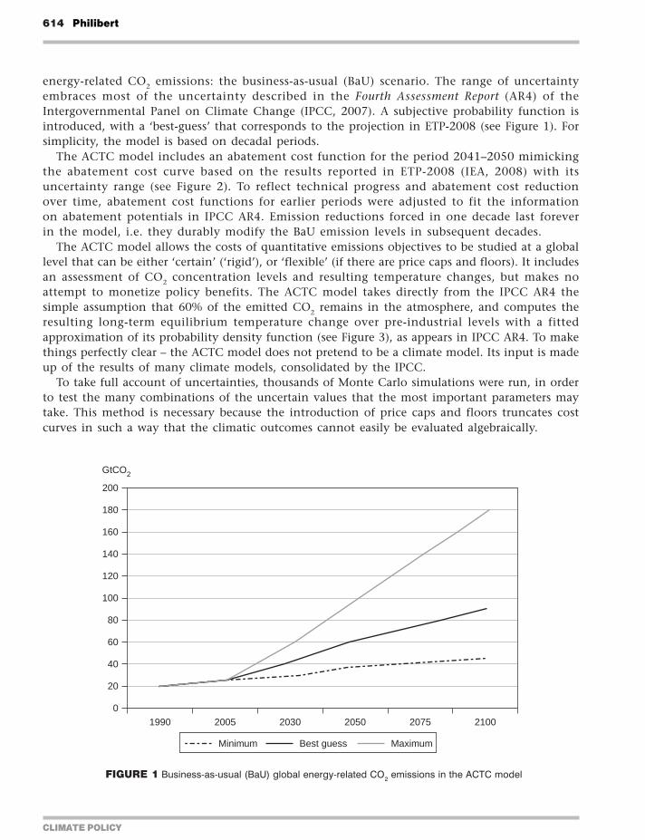
CLIMATE POLICY

614 Philibert

energy-related CO2 emissions the business-as-usual (BaU) scenario The range of uncertaintyembraces most of the uncertainty described in the Fourth Assessment Report (AR4) of theIntergovernmental Panel on Climate Change (IPCC 2007) A subjective probability function isintroduced with a lsquobest-guessrsquo that corresponds to the projection in ETP-2008 (see Figure 1) Forsimplicity the model is based on decadal periods

The ACTC model includes an abatement cost function for the period 2041ndash2050 mimickingthe abatement cost curve based on the results reported in ETP-2008 (IEA 2008) with itsuncertainty range (see Figure 2) To reflect technical progress and abatement cost reductionover time abatement cost functions for earlier periods were adjusted to fit the informationon abatement potentials in IPCC AR4 Emission reductions forced in one decade last foreverin the model ie they durably modify the BaU emission levels in subsequent decades

The ACTC model allows the costs of quantitative emissions objectives to be studied at a globallevel that can be either lsquocertainrsquo (lsquorigidrsquo) or lsquoflexiblersquo (if there are price caps and floors) It includesan assessment of CO2 concentration levels and resulting temperature changes but makes noattempt to monetize policy benefits The ACTC model takes directly from the IPCC AR4 thesimple assumption that 60 of the emitted CO2 remains in the atmosphere and computes theresulting long-term equilibrium temperature change over pre-industrial levels with a fittedapproximation of its probability density function (see Figure 3) as appears in IPCC AR4 To makethings perfectly clear ndash the ACTC model does not pretend to be a climate model Its input is madeup of the results of many climate models consolidated by the IPCC

To take full account of uncertainties thousands of Monte Carlo simulations were run in orderto test the many combinations of the uncertain values that the most important parameters maytake This method is necessary because the introduction of price caps and floors truncates costcurves in such a way that the climatic outcomes cannot easily be evaluated algebraically

01990 2005 2030 2050 2075 2100

20

40

60

80

100

120

140

160

180

200

GtCO2

Minimum Best guess Maximum

FIGURE 1 Business-as-usual (BaU) global energy-related CO2 emissions in the ACTC model

Assessing the value of price caps and floors 615

CLIMATE POLICY

22 Halving global energy-related emissions by 2050The IPCC AR4 considers emission reductions to 50ndash85 below 2000 levels to be compatible withstabilized CO2 concentrations of 350ndash400 ppm or all GHG concentrations (in CO2-eq) of 445ndash490 ppm and a global mean temperature increase of 2degCndash24degC above pre-industrial temperaturesat equilibrium using lsquobest-estimatersquo climate sensitivity

The G8 leaders at their meeting at Toyako (Japan) in July 2008 declared that they

seek to share with all Parties to the UNFCCC the vision of and together with them to consider andadopt in the UNFCCC negotiations the goal of achieving at least 50 reduction of global emissionsby 2050 (G8 Leaders 2008)

50 900 50

201 564

1 2 3 4 5 6 7 80

Mod

e =

299

13

FIGURE 3 Climate sensitivity in the ACTC model (in degrees Celsius)

ndash

ndash

200

100

0

100

1 8 15 22 29 36 43 50 57 64 71 78 85 92 99 106

113

120

127

134

141

148

155

200

300

400

500

600

US$

2041ndash2050 high Best guess 2041ndash2050 low

FIGURE 2 Marginal abatement cost (MAC) in the ACTC model for the period 2041ndash2050

CLIMATE POLICY

616 Philibert

The analysis focuses on at least halving global emissions by 2050 and investigates whether somelower emission levels could be achieved for similar expected costs if price caps and floors wereintroduced into the global architecture

Philibert (2008) suggests that the main criterion to assess policies is the lsquowarming committed by2050rsquo ndash ie the long-term equilibrium warming that would result from a stabilization of CO2

concentrations at the level reached by 2050 This concept is of course different from lsquotransientwarmingrsquo ndash ie the warming actually realized at that date ndash due to the thermal inertia of theoceans and land masses

In this article however the main criterion used is the warming committed by 2100 The ACTCmodel was extended to 2100 with respect to the analysis of CO2 concentration and climate outcomesThus except for the lsquoNo policyrsquo case all the results presented in this article rest on a similaradditional assumption that the remaining emissions are progressively eliminated between 2050and 2100 This extension provides a clearer picture of the climate outcomes of the various climatepolicies considered on a time horizon that corresponds to achieving atmospheric CO2 stabilizationHowever given the lack of robust information with respect to abatement costs beyond 2050 thisprogressive elimination is not accounted for in the cost assessments which are therefore limitedto the period 2011ndash2050

23 Differences from earlier studiesPrevious research has attempted to assess the introduction of price caps in global mitigationarchitecturesdomestic emissions trading schemes In particular Pizer (2002) building on Weitzman(1974) showed that in the case of climate change introducing price caps reduces expected coststo a much greater degree than it reduces expected benefits as a result expected net benefits(welfare gains) would be five times greater with flexible targets (or carbon taxes) than with rigidtargets

Pizer (2003) further explored the conditions under which rigid quantitative targets might stillbe preferred He showed that severe catastrophic climate damage triggered by known GHGconcentration thresholds may indeed call for purely quantitative targets

There are two main differences between the present study and Pizerrsquos Spelling out these differencesmay help to achieve a clearer understanding of the aims of this study They are as follows

Pizer considered the difficulty of choosing a discount rate as a major source of uncertaintywhich explains about half the increase in expected net benefits of climate policy due toprice caps The ACTC model uses a 5 discount rate thereby focusing on other sources ofuncertainty

Pizer offered views on the optimal level of abatement and looked for the optimal setting oftargets and price caps or taxes This study takes the aim of halving emissions by 2050 forgranted and only questions whether such an objective must be reached with a great level ofprecision and certainty despite uncertain abatement costs or not This aim correspondswith an expected amount of expense that the international community may find acceptableto spend to mitigate climate change risks our study seeks the most cost-effective use of thatmoney

There are two possible rationales for setting more ambitious targets after price caps are introduced(1) if the objective is to maintain optimality in setting targets one should introduce price floorsif price caps have been included If price floors are deemed politically or financially difficult to

Assessing the value of price caps and floors 617

CLIMATE POLICY

introduce their absence must be compensated for by some tightening of the original targets(Cournegravede and Gastaldo 2002) (2) If the uncertainty about marginal benefit is too lsquodeeprsquo andthere is no real best guess (Schneider 2003) the idea is to maximize the environmental benefitsfor the same anticipated costs Even if price floors are introduced tightening the original targetsstill makes sense A first step is to search for the target that provides the same expected climaticresults with caps and floors ndash and lower expected costs A second step is to look for the target thatentails the same expected costs but with better climate outcomes (Philibert 2006)

3 lsquoNo policyrsquo case and rigid targets

In this section we briefly assess the climate outcomes that would result from the absence of anypolicy to mitigate climate change and the costs and climate consequences of setting and achievingthe rigid target of halving global emissions by 2050

31 lsquoNo policyrsquo caseIn the absence of policy global energy-related CO2 emissions would continue to grow reachingunder best guess 42 Gt CO2 by 2030 60 Gt CO2 by 2050 and 90 Gt CO2 by 2100 This would leadto CO2 concentrations of 534 parts per million (ppm) by 2050 and 820 ppm by 2100 under best-guess estimates

Running 3000 Monte Carlo simulations with the ACTC model shows CO2 concentrations inthe range of 662ndash1067 ppm by 2100 Figure 4 represents the probability distribution of thetemperature change committed by 2100 in the lsquoNo policyrsquo case (temperature changes in degreesCelsius are in abscissa the taller the bar the greater the probability) There is virtually no chancethat the warming does not exceed 2degC and less than a 20 chance that it does not exceed 4degCThere is a 50 risk that the warming exceeds 525degC (median value) There is an 188 risk thatthe warming exceeds 7degC the lsquoNo policyrsquo scenario therefore looks like a lsquoNo futurersquo scenarioUndertaking no policy is not an option

197 614 188

400

Rel

ativ

e pr

obab

ility

700

0 2 4 6 8 10 12 14 16

Med

ian

= 5

2517

degC

FIGURE 4 Warming committed by 2100 in the lsquoNo policyrsquo case

CLIMATE POLICY

618 Philibert

32 Setting intermediate targetsOn the basis of the G8 final communiqueacute in Toyako (G8 Leaders 2008) we want to halve globalenergy-related CO2 emissions by 2050 The communiqueacute did not specify any reference level so weassume it could be close to the level of emissions known at the time and we take as reference the2005 level We factor a target of 13568 Gt CO2 for 2050 or more precisely for the period 2041ndash2050 From this important mid-point we proceed backward to establish a full set of decadaltargets to stabilization by 2010 That is the model is run to find the intermediate target values(2011ndash2020 2021ndash2030 and 2031ndash2040) that minimize the net present value of overall abatementcosts until 2050 We first ignore the uncertainty ie we use only best-guess values

Table 1 shows the allowed emissions percentage of reference levels marginal abatement costs(MAC) and total abatement costs (TAC) for the optimal pathways towards 2050 levels for thetarget studied According to such pathways global emissions would optimally peak at some pointbetween 2011 and 2020 This is in line with IPCC (2007)

33 Halving global emissions from 2005 levels straight targetsLet us now run again 3000 Monte Carlo simulations GDP growth rate per decade and carbonintensity and also coefficients driving the MAC curve take random values No price cap is factoredin yet We then look at the cost outcomes ndash MAC TAC during the first period 2021ndash2020 netpresent value of total abatement costs to 2050 in absolute terms and in percentage of GDP ndash whenhalving global emissions by 2050 from both 2005 levels and 1990 levels

Figure 5 shows the net present value of total abatement costs until 2050 This has a mean valueof US$7885 billion against a best-guess value of US$2754 billion The expected value whenuncertainty is taken into account is thus basically three times larger than when it is not This ofcourse is a very important result in itself which results from the steep slopes of the marginalabatement cost curves and the breadth of the uncertainty particularly with respect to BaUemissions The savings when BaU emissions are less than expected are much smaller than theadditional costs incurred when BaU emissions are more than expected

It is also interesting to consider total abatement costs in percentage of the world gross product(WGP) The mean value is 039 and the considerable dispersion extends from ndash0019 to +547

A closer look at the first period 2011ndash2020 reveals that MAC have a mean or average value ofUS$92 which is roughly 40 higher than the best-guess value of US$67 This stems from thesteepness of the MAC function higher-than-expected unabated emissions increase MAC muchmore than lower-than-expected unabated emissions reduce MAC

TABLE 1 Intermediate objectives for halving emissions by 2050 from 2005 levels

2011ndash2020 2021ndash2030 2031ndash2040 2041ndash2050 Total (NPV)a

Reference 2005 94 835 745 50

Cap (Gt CO2) 257835 234156 206237 135680 8339

MAC ($t CO2)b 67 101 158 252

TAC (bn $)c 350 1119 3002 6575 2754

a NPV = Net present valuebMAC = Marginal abatement costscTAC = Total abatement costs

Assessing the value of price caps and floors 619

CLIMATE POLICY

Uncertainties have a more dramatic effect when TAC for the same 2011ndash2020 period are computedas apparent in Figure 6 The mean value is US$929 billion ndash whereas it was only US$350 billionunder best-guess values for all parameters Total costs are computed as an integral of the marginalcost function and thus grow faster than marginal costs when the required abatement augmentsTable 2 summarizes the expected MAC TAC and TAC in proportion to the GDP during theperiods following to 2050 by comparison with the best-guess values while halving global emissionsfrom 2005 levels It is worth noting that although mean values are several times higher thanbest-guess values the percentage of total expected costs does not exceed (on average) 1 of expectedGDP in any period ndash a result that is consistent with the Stern Report (2006)

Let us now consider the environmental results of this policy to 2100 As emissions over thiscentury are known with quasi-certainty1 the CO2 concentration reached by 2050 is known to be484 ppm or very close to 484 ppm The results for temperature change however reflect the uncertaintythat affects the equilibrium temperature change in the IPCC AR4 (Figure 7) When compared with

50 900 50

04 245

ndash20 0 20 40 60 80 100 120 140 $bn times 1000

Mea

n =

7884

885

4

Rel

ativ

e pr

obab

ility

FIGURE 5 Net present value (NPV) of abatement costs to 2050 (no price cap)

Note Mean value is in $bn

50 900 50

ndash2 0 3 4 6 8 10 12 14

ndash029 406

Mean =

9289

778

Rela

tive p

robabili

ty

$bn times 1000

FIGURE 6 Total abatement costs in the period 2011ndash2020 (no price cap)

Note Mean value is in $bn

CLIMATE POLICY

620 Philibert

the lsquoNo policyrsquo case these results are important The median value of warming committed by 2100is down from 525degC to 272degC The chance of not exceeding 2degC is now 158 and the risk ofexceeding 4degC is down from 803 to 112 The risk of exceeding 7degC has been virtually eliminated

4 Assessing price caps and price floors

In this section we introduce price caps during the four periods to 2050 testing various levels to find out thelikely effects on both abatement costs and actual emissions We tighten the targets and introduce pricefloors with the same purpose We then seek the combination of targets price caps and floors that would leadto similar environmental results ndash starting with the same average concentration levels Then we search forthe combination that would entail the same expected costs presumably with better environmental results

TABLE 2 Marginal and total abatement costs to 2050 of halving CO2 from 2005 levels

2011ndash2020 2021ndash2030 2031ndash2040 2041ndash2050 Total (NPV)a

MAC ($t)b Best guess 67 101 158 252

Mean 92 181 288 504

TAC (bn$)c Best guess 350 1119 3002 6575 2754

Mean 929 3729 8307 18179 7885

TAC in WGPd Best guess 004 010 020 033

Mean 011 030 050 080 039

a NPV = Net present valueb MAC = Marginal abatement costsc TAC = Total abatement costsd WGP = World gross product

158 729 112

200 400

0 1 2 3 4 5 6 7 degC

Med

ian

= 2

7159

Rel

ativ

e pr

obab

ility

FIGURE 7 Warming committed by 2100 rigid targets of half 2005 levels

Assessing the value of price caps and floors 621

CLIMATE POLICY

Price caps could be simple compliance payments to governments (for domestic sources) andorto some international entity (for governments) at the end of commitment periods ndash at prices setup and known by all at their outset Price floors could be reserve prices in periodic auctioningthus creating no liability for government (no need for subsidies)

41 lsquoLowrsquo price capsLet us test two different price cap schedules We name the first lsquolow price capsrsquo as they aredeliberately set about one-third below MAC in each period The second lsquohigh price capsrsquo is setabout 50 higher than the MAC in each period

We define lsquolowrsquo price caps at US$40 60 80 and 100 respectively in the four periods and runthe model 3000 times Total expected abatement costs during the first period are considerablyreduced ndash indeed they become negative at ndashUS$34 billion as energy savings (negative to no costoptions) are more important than positive costs of other emissions reductions

However emissions during the first period 2011ndash2020 are on average about 12 Gt CO2 higherthan the 257835 Gt CO2 target and in about 10 of the cases are 30 Gt CO2 above the target asshown in Figure 8 (the highest bar shows the probability of achieving the target while the lowerbars to the right show the frequency of outcomes when the price caps lsquokick inrsquo)

The deviation from the desired emission trajectory increases over time and in the last period2041ndash2050 emissions are considerably above the target (136 Gt CO2 in 10 years) at 222 Gt CO2 onaverage ndash a 63 increase ndash and twice as high in about 20 of the cases

Over the entire period 2011ndash2050 the net present value of total expected abatement costs isdown to US$645 billion a sharp reduction from the case with straight targets The nature of thisreduction in expected costs is further discussed in Section 43

CO2 concentrations range from 482 to 544 ppm by 2100 If the most likely outcome is 482 ppm themean value is 498 ppm ndash against 484 ppm in the previous case This relatively modest difference illustratesthe cumulative nature of the climate change issue deviations of 63 in emissions (2041ndash2050) end upwith a 3 increase in concentrations The warming committed by 2100 has a median value of 285degC(Figure 9) There is a 125 chance of not exceeding 2degC and a 148 risk of exceeding 4degC

These results are considerably more favourable to the environment than the lsquoNo policyrsquo caseThey reveal however some degradation of environmental outcomes when compared with rigid

00 895 105

2575

250 260 270 280 290 300 310 320GtCO2

2875

Mea

n =

269

3543

Rel

ativ

e pr

obab

ility

FIGURE 8 Actual emissions 2011ndash2020 with US$40 price cap

CLIMATE POLICY

622 Philibert

targets lsquoLow-levelrsquo price caps do reduce expected costs and the cost uncertainty of climate policybut weaken its environmental results though perhaps less than expected It must be emphasizedhowever that these lsquolow-levelrsquo price caps remain relatively consistent with the ambition of thetargets If price cap levels were set at significantly lower levels they would probably drive muchmore substantial deviations of the climatic outcomes

42 lsquoHighrsquo price capsWe set price caps at high levels ndash US$110 150 230 and 350 respectively ndash for each period Expectedcosts during the first period reach US$428 billion ndash about half their initial level Emissions duringthat period remain higher than the target at 261 Gt CO2 Emissions during the 2041ndash2050 periodhave a mean value of 164 Gt CO2 which is about 20 above the target (Figure 10) Even relativelyhigh price caps create a significant deviation from the desired objectives

125 728 148

200 400

0 1 2 3 4 5 6 7 8degC

Med

ian

= 2

8458

Rel

ativ

e pr

obab

ility

FIGURE 9 Warming committed by 2100 with lsquolowrsquo price caps

00 950 50

1350 2546

100 150 200 250 300 350 400 450 500

GtCO2

Mea

n =

164

1191

Rel

ativ

e pr

obab

ility

FIGURE 10 Actual emissions 2041ndash2050 with lsquohighrsquo price caps

Assessing the value of price caps and floors 623

CLIMATE POLICY

Over the entire period 2011ndash2050 total expected costs have a net present value of US$2925 billionCO2 concentrations by 2100 are in the range 481ndash531 ppm with a mean value of 489 ppmTemperature change has a median value of 276degC as can be seen from Figure 11 which is stillabove the result with a rigid target though the difference has narrowed

43 Price caps and price floorsLet us now consider combining lsquomiddlendashhighrsquo price caps (somewhat above the best-guess marginalabatement costs in each period) and price floors (somewhat below the same costs) We set pricecaps at US$80 120 180 and 260 for the periods 2011ndash2020 2021ndash2030 2031ndash2040 and 2041ndash2050respectively and price floors at half these levels ie US$40 60 90 and 130

Emissions during the first period have a mean value of 2601 Gt CO2 which is only 1 abovethe 257835 Gt CO2 target The deviation is much smaller with price floors than without them Inabout 24 of the cases the target is exceeded by 1 Gt CO2 per year or more while in about 134of the cases emissions are 1 Gt CO2 per year below the target (Figure 12) Abatement costs aredown to US$297 billion ndash one-third of their initial value

Emissions during the last decade before 2050 have a mean value of 1605 Gt CO2 still higher thanthe 13568 Gt CO2 target which is reached or exceeded in 437 of the cases The price floor evenmakes it possible that emissions come down to zero though the probability is low and requires thecombination of an extremely low BaU trend with the lowest possible MAC There is a 57 riskhowever that emissions are twice as much or more than the target (Figure 13)

Over the entire period to 2050 the net present value (NPV) of total expected abatement costs isUS$2292 billion This interesting result shows the usefulness of price floors In comparison withhigh price caps total costs are reduced by 216 (US$2292 billion vs US$2925 billion) Stillconcentration results are slightly better by 2100 in the range 441ndash528 ppm with a mean value of488 ppm

Probably no less important from a political standpoint is the sharp reduction in cost uncertainty ndashnot only expected costs When expressed in percentage of the world gross product the range oflikely costs of mitigating climate change which with rigid targets extended from 0 to 55 hasnarrowed from 0 to 02

146 731 123

200 400

0 1 2 3 4 5 6 7 8

Med

ian

= 2

7550

Equilibrium temperature change 2100

ordmC

Rel

ativ

e pr

obab

ility

FIGURE 11 Warming committed by 2100 with lsquohighrsquo price caps

CLIMATE POLICY

624 Philibert

Results expressed in temperature changes are worth considering (Figure 14) as they are fairlyclose to those obtained with rigid targets though not exactly the same with a median temperaturechange of 275degC vs 272degC with rigid targets

The results warrant closer examination A reduction in expected costs to one-third and anarrowing of the uncertainty range by one order of magnitude while keeping the climatic resultsalmost the same may seem lsquotoo good to be truersquo and needs some explanation Price caps do notreduce the actual costs ndash when the uncertainty is resolved However they do reduce the expectedcosts which have been computed taking the uncertainties into account ndash the only costs that therational decision-makers should consider

As seen above the expected costs are about three times greater than the lsquobest-guessrsquo abatementcosts calculated when one selects the best-guess value for each parameter The steepness of themarginal cost curve ndash a cost that increases rapidly with the amount of abatement required to

134 626 240

2475 2675

220 230 240 250 260 270 280 290 300 310M

ean

= 26

010

77

GtCO2

Rel

ativ

e pr

obab

ility

FIGURE 12 Actual emissions 2011ndash2020 with US$80 price cap and US$40 price floor

437 506 57

1357 2714

0 50ndash50 100 150 200 250 300 350 400 450 500

Mea

n =

160

4841

GtCO2

Rel

ativ

e pr

obab

ility

FIGURE 13 Actual 2041ndash2050 emissions with price caps and price floors

Assessing the value of price caps and floors 625

CLIMATE POLICY

achieve the fixed target ndash combines with the breadth of the uncertainties notably those relativeto economic growth and BaU emissions to explain this result When price caps are introduced atlevels close to those of the marginal abatement costs in each decadal period they somehow bringthe expected costs close to the best-guess costs ndash three times smaller

Meanwhile the price floor reduces emissions beyond the quantitative targets when costs aresmall They increase the costs attached to a given target but as they help maintain a symmetry ofthe possible emission outcomes around the target they do reduce the expected costs of achieving(in probabilistic terms) given emission concentration and finally temperature change outcomes

These results however are dependent on the assumptions of the model To replicate the marginalcost curve of ETP-2008 numerical functions were introduced to compute the MAC as a functionof the amount of abatement in each decade After some point these costs grow rapidly andcontinue to grow when the amount of the required abatement exceeds what is considered in ETP-2008 which had only one scenario for BaU emissions Indeed there is little information either tovalidate or invalidate the choice of not introducing another lsquokinkrsquo in that curve which couldreflect for example a so-called lsquoback-stoprsquo technology It might be modified however in thepresence of new information If there were a back-stop technology to cap the costs of emissionsreduction introducing price caps would obviously be less useful

Finally because climate change is driven not by emissions themselves but by their slowaccumulation in the atmosphere price-driven variations in decadal emissions which can be onthe high or the low side tend to cancel out The additional uncertainty introduced withconcentration is small compared with the uncertainty of the Earthrsquos climate sensitivity and makingthe target slightly more ambitious may allow as we will see now in probabilistic terms obtainingsimilar or even slightly better climate results for much lower expected costs

44 More ambitious target with price cap and price floorsWe now try to achieve the same environmental results as with rigid targets For example we chooseto reduce emissions by half from 1990 levels by 2050 as suggested by the European Union whilekeeping the price cap and price floor at the same levels as in the previous case The assumption here

153 728 119

200 400

0 1 2 3 4 5 6 7 8degC

Med

ian

= 2

7463

Rel

ativ

e pr

obab

ility

FIGURE 14 Warming committed by 2100 with price caps and price floors

CLIMATE POLICY

626 Philibert

is that controlling the marginal costs is what matters as this is how the public at large will perceivethe maximum cost incurred because it can easily be translated into costs per barrel of oil litre orgallon of gasoline or electrical kWh ndash in the latter case depending on the mix and efficiency of thepower generation For example US$80 per tonne of CO2 translates into about US$019 per litre ofgasoline and about US$0056 per kWh in the USA or US$004 (euro0028 as at 1 July 2009) in the EUHence we first consider tightening the target while keeping price caps and floors at the same levels

The total expected costs increase to US$2553 as the target gets more ambitious but they remainlower than with the unmodified target and the high price caps but no price floor and of coursemuch lower than with the unmodified target and no price cap at all The concentration reachedby 2100 extends from 443 to 525 ppm with a mean value of 482 ppm In terms of temperaturechange the results as shown in Figure 15 are slightly better than those obtained with the rigidtargets that led to a concentration of 484 ppm (as shown in Figures 2ndash4) Achieving a givenconcentration level exactly or on average does not make any real difference in the environmentaloutcome The uncertainty introduced by price caps in concentration levels is entirely maskedbehind the uncertainty on climate sensitivity

These results confirm those of earlier qualitative analyses Uncertain emission outcomes over adecade due to price caps create less uncertainty on concentration levels while GHGs slowlyaccumulate in the atmosphere Further this uncertainty on concentration levels is essentiallyunnoticeable in the final analysis in terms of temperature change ndash whether one considers medianvalues or the risk of exceeding specific values Uncertainty on equilibrium temperature change byfar dominates uncertainty on concentration levels

Another possibility is to increase the price cap and floor levels after the target has been mademore ambitious to better fit the new marginal abatement cost schedule This allows for findingmore climate-friendly combinations of caps and floors with the same target of halving globalenergy-related CO2 emissions by 2050 from 1990 levels

45 Symmetric safety valve and quasi-carbon taxHere price caps are set at 150 of the best-guess MAC and price floors are symmetrically set at50 of the best-guess MAC2 The total expected costs of that policy would be US$4638 billion

168 725 106

200 400

0 1 2 3 4 5 6 7degC

Med

ian

= 2

6916

Rel

ativ

e pr

obab

ility

FIGURE 15 Warming committed by 2100 with a target of half 1990 levels price caps and floors

Assessing the value of price caps and floors 627

CLIMATE POLICY

which is significantly higher than in the previous cases though still lower than with rigid targetsThe concentration by 2100 would range from 444 to 517 ppm with a mean value of 476 ppmThe temperature change committed by 2100 would have a median value of 263degC ndash an improvementover all previous attempts

The ACTC model also allows for modelling a carbon tax or a quasi-carbon tax The lsquomanaged-price approachrsquo proposed by the Congressional Budget Office in the USA (Elmendorf 2009) couldprobably also be analysed in the same way It suffices to set price caps and price floors at almostthe same levels Running it with the more ambitious target (halving emissions by 2050 from 1990levels) and price caps and floors set with US$1 difference above and below the best-guess marginalcosts resulting from this target3 yields interesting results

Of course there would be many differences between a large price corridor and a very narrowone as illustrated by the two cases offered here In the first case trading would occur while in thesecond there would be very little trading if any An assessment of these differences is beyondthe scope of this article But it is interesting to test the carbon tax or similar instruments using thesame methodology

A quasi-carbon tax would reduce total abatement costs by comparison with the previous caseas they would reach US$4212 billion A considerable dispersion in emission possibilities in eachdecade before 2050 leads to the greatest dispersion of concentration outcomes from 424 to 530 ppmby 2100 with a mean value of 475 ppm The results (shown in Figure 16) are even slightly betterthan with the symmetric safety valve with a committed temperature change of 262degC (medianvalue) by 2100

46 Still more ambitious targets price caps and price floorsWe now attempt to find a combination of targets that would entail the same expected costs asrigid targets ndash and presumably deliver better environmental results

One combination that goes a long way in that direction consists in setting the 2050 target at aquarter of 1990 levels or 526 Gt CO2 in 10 years Optimal intermediate targets are computed tominimize the net present value of abatement costs to 2050 using best-guess values

193 712 95

200 400

0 1 2 3 4 5 6 7 8degC

Med

ian

= 2

6191

Rel

ativ

e pr

obab

ility

FIGURE 16 Warming committed by 2100 with a quasi-tax

CLIMATE POLICY

628 Philibert

Price caps are set at US$150 240 360 and 600 which are slightly above the best-guess MACresulting from that ambitious objective Price floors are set at US$50 80 120 and 200 for theperiods 2011ndash2020 2021ndash2030 2031ndash2040 and 2041ndash2050 respectively

Emissions end up on average at 88 Gt CO2 in the period 2041ndash2050 or 43 of 1990 levels (30of 2005 levels) as shown in Figure 17 The ambitious target is reached in about 40 of the casesThere is a 17 chance that the original rigid target of half 2005 levels is exceeded

The net present value of expected abatement costs to 2050 is US$6762 billion ndash still lower thanhalving emissions from 2005 levels with certainty Concentrations by 2100 end up in the range440ndash498 ppm with a mean value of 462 ppm The resulting temperature change committed by2100 shows a median value of 249degC the chance of not exceeding 2degC is 241 the risk ofexceeding 4degC is 73 (Figure 18)

396 431 174

526 1360

0ndash50ndash100 50 100 150 200 250 300 350

Mea

n =

878

064

GtCO2

Rel

ativ

e pr

obab

ility

FIGURE 17 Actual emissions 2041ndash2050 with target 25 of 1990 levels price caps and floors

241 686 73

200 400

0 1 2 3 4 5 6 7degC

Med

ian

= 2

4894

Rel

ativ

e pr

obab

ility

FIGURE 18 Warming committed by 2100 with target 25 of 1990 levels price caps and floors

Assessing the value of price caps and floors 629

CLIMATE POLICY

47 Allowance reserveFinally the ACTC model was modified to simulate an allowance reserve as suggested by Murrayet al (2009) The additional allowances in the reserve would be put on the market if the carbonprice reaches some trigger level however if the reserve is exhausted the price is no longer limitedThe system behaves like a lsquolimitedrsquo price cap system In the framework of targets set to halveglobal energy-related CO2 emissions by 2050 from 2005 levels with price caps and price floorssimilar to those described at the beginning of this section an allowance reserve set at 10 of totalamount of allowances for a given period was tested Figure 19 shows its effects on the distributionof emission outcomes

A growing reserve from 10 to 25 of allowed emissions was also tested The results areshown in Table 3 and compared with those obtained with a more ambitious policy (halvingglobal emissions from 1990 levels) and plain price caps This shows that more ambitious policieswith unlimited price caps and price floors might be preferable to schemes with price caps limitedin size due to an allowance reserve

TABLE 3 Allowance reserve vs (unlimited) price caps

Policy Price caps Discounted abatement Warming committed by

Price floors costs to 2050 (mean) 2100 (median)

Rigid targets None $7885 billion 272degC

None

10 allowance reserve $80ndash260 $6282 billion 271degC

$40ndash130

Growing reserve (10ndash25) $80ndash260 $5122 billion 272degC

$40ndash130

Tighter targets $80ndash260 $2553 billion 269degC

Unlimited price caps $40ndash130

FIGURE 19 Emissions 2011ndash2020 with a 10 allowance reserve

50 900 50

2404 2828

220 230 240 250 260 270 280 290

Mea

n =

259

9555

GtCO2

Rel

ativ

e pr

obab

ility

CLIMATE POLICY

630 Philibert

5 Discussion and conclusions

A number of observations can be made from these results summarized in Table 4 The first is thatmitigation action whatever its form and costs makes an enormous difference in the resultingclimate change by the end of this century

The second is that given the spread of the uncertainties relative to unabated emission trendsand abatement costs price caps can significantly reduce cost uncertainty and expected costs ndash byup to two-thirds according to the assumptions of the model Meanwhile price floors help tomaintain the environmental effectiveness of the policy Price floors increase the costs attached tosome targets but contribute to keeping the costs low in achieving a given environmental result

Price-driven variations in emissions have little influence on policy outcomes (temperaturechange) if price cap and price floor levels are roughly consistent with the ambition of the policyAs previously pointed out by Pizer (2002) and Newell and Pizer (2003) this is primarily explainedby the stock nature of the issue of climate change the slow build-up of CO2 concentrationssmoothes short-term emission changes Our results further point to the role of uncertainty on theEarthrsquos climate sensitivity which by far exceeds and in some ways masks the uncertainty onemission levels

Tighter targets with price caps and price floors entail lesser economic risks and similar or slightlybetter climate results For example halving emissions by 2050 from 1990 levels with price caps andfloors offers similar environmental results as halving emissions from 2005 levels with straighttargets ndash but for one-third of the (expected) costs according to the assumptions of the modelAlternatively a significantly more ambitious target could be chosen with better climatic resultswith expected costs still lower than those implied by a rigid but less ambitious target

TABLE 4 Summary of results

Half 2005 level

Half 2005 +price caps amp

floors

Half 1990 +caps amp floors

Half 1990 +caps amp floors

Quasi tax(half 1990)

Tighter target+ caps amp floors

Assessing the value of price caps and floors 631

CLIMATE POLICY

With respect to economic risks taxes are similar to permits with price corridors and bothdominate straight targets In a recent defence of emissions trading Nathaniel Keohane (2009)notes however that taxes may focus the public debate on the cost of abatement while quantitativetargets may focus it on the lsquocaprsquo or the environmental necessity of addressing the threat ofclimate change Hopefully price caps could be less prone to such a psychological effect as theywould be part of hybrid instruments together with emission targets and price floors (which mayhelp avoid a cap on the marginal abatement cost being mistaken for a cost)

In these results the reduction of expected costs can only partly result from so-called timeflexibility Banking and borrowing for example could reduce expected costs if the volatility ofcarbon prices is due to successive economic shocks of opposite signs If however BaU emissionsover time show a progressive departure from expectations being constantly above or belowexpected trend time flexibility will do little or nothing to reduce costs if at the end of the dayall deviations from targets must be corrected and the lsquointegrityrsquo of the targets must be restored(see Fell et al 2008)

In running the ACTC model with price caps and floors the reduction in expected costs resultsprimarily from the flexibility given to adjusting the emission levels to the actual abatement costsThis is also what makes it difficult to accept by many However this is a logical consequence ofaccepting that abatement costs are considered in defining the level of abatement If only benefitswere considered the optimal emission level would be the lowest one ndash for the sake of the climateit would be better to halt GHG emissions right away But this is usually not considered possiblefor the costs would be too important

However if abatement costs are considered in setting the objective then it is legitimate toadjust the level of abatement to those costs Uncertainties prevent performing ex ante a full costndashbenefit analysis To some extent the difficulties in assessing the monetary value of the damageassociated with climate change are likely to persist Nevertheless as abatement costs are consideredin setting quantitative emissions targets it seems legitimate to adjust them if these costs deviatefrom expectations This is what price caps and floors do in a manner that remains predictable byinvestors and does not undermine the confidence that market players may have in the stability ofclimate change mitigation policies

In conclusion short-term certainty on emissions appears less important than long-term policyambition The usual criticism is that marginal damage from climate change may be highly non-linear and grow very rapidly beyond some thresholds This would justify the choice of a policydelivering guaranteed results such as straight targets of firm caps on emissions However Pizer (2003)showed that there would be a preference for straight targets only if the thresholds themselves ndash forexample GHG concentration thresholds ndash were known with full certainty If this is not the casethe most ambitious policy remains preferable

This appears all the more true if as is likely the non-linear damage would be triggered bytemperature change Price caps and floors seem appropriate in order to help governments acceptslightly more ambitious policies Given the uncertainty on the Earthrsquos climate sensitivity thesepolicies may have slightly better expected results than the policies with more lsquocertainrsquo results dueto straight targets Despite the flexibility allowed in emission levels the lsquomore ambitious lesscertainrsquo policies are in practice less likely to meet the unknown temperature change level thatwould trigger these most-feared non-linear damages

This quantitative assessment however does not provide all the answers It is limited to carbondioxide emissions from fossil fuel combustion It does not address the effects of limiting pricevolatility on investorsrsquo behaviour Nor does it address complex implementation issues related tolinking a global international regime with domestic nation-wide emissions trading schemes or

CLIMATE POLICY

632 Philibert

linking these schemes altogether when price caps and price floors are involved These issues requirefurther work

Acknowledgements

The views expressed here are those of the author and do not necessarily represent those of theIEA the OECD or their Member States I would like to express my gratitude to those whocontributed to this research in 2009 with their support comments criticisms or suggestions inparticular Paolo Frankl Brice Lalonde Claude Mandil Larry Goulder John Weyant MartyWeitzman Rob Stavins Charles Graves Metin Celebi Gregory Nemet Jake Jacoby DennyEllerman Richard Newell Jonathan Wiener Brian Murray Terry Dinan Dick MorgensternDallas Burtraw Harrison Fell Sacha Golub Nat Keohane Cathleen Kelly Richard Lorch andthree anonymous referees

Notes

1 There is a small probability that BaU emissions close to the end of the century could fall below target emissions asa result of the emission reductions undertaken in the early decades of the century but which because of how themodel is constructed permanently modify the BaU emission trajectory

2 The price caps would be set at US$132 per tonne CO2 in 2011ndash2020 US$202 in 2021ndash2030 US$318 in 2031ndash2040and US$511 in 2041ndash2050 Price floors would be set at US$44 in 2011ndash2020 US$67 in 2021ndash2030 US$106 in 2031ndash2040 and US$170 in 2041ndash2050

3 In this case price caps and floors would respectively be set at US$88 and 87 in 2011ndash2020 US$135 and 134 in 2021ndash2030 US$213 and 212 in 2031ndash2040 and US$342 and 341 in 2041ndash2050

References

Burtraw D Palmer K Kahn D 2009 A Symmetric Safety Valve Resources for the Future Washington DC [availableat wwwrfforgNewsFeaturesPagesA_Symmetric_Safety_Valveaspx]

Cournegravede B Gastaldo S 2002 lsquoCombinaison des instruments prix et quantiteacutes dans le cas de lrsquoeffet de serrersquoEacuteconomie et Preacutevision 156 2002ndash2005

Elmendorf DW 2009 Flexibility in the Timing of Emission Reductions Under a Cap-and-Trade Program Testimony beforethe Committee of Ways and Means US House of Representatives Congressional Budget Office [available atwwwcbogovdoccfmindex=10020]

Fell H Morgenstern RD 2009 Alternative Approaches to Cost-Containment in a Cap-and-Trade System Resources forthe Future Washington DC [available at wwwrfforgPublicationsPagesPublicationDetailsaspxPublicationID=20779]

Fell H McKenzie IA Pizer WA 2008 Prices versus Quantities versus Bankable Quantities Resources for the FutureWashington DC [available at wwwrfforgPublicationsPagesPublicationDetailsaspxPublicationID=20557]

G8 Leaders 2008 G8 Hokkaido Toyako Summit Leadersrsquo Declaration [available at wwwmofagojppolicyeconomysummit2008docdoc080714_enhtml]

Golub A 2009 Price Caps and Price Floors in Climate Policy Comments Presentation at the Center for Energy MarineTransportation and Public Policy Columbia University New York

IEA 2008 Energy Technology Perspectives Scenarios and Strategies to 2050 IEA ParisIPCC (Intergovernmental Panel on Climate Change) 2007 Fourth Assessment Report Synthesis Report GenevaKeohane NO 2009 lsquoCap and trade rehabilitated using tradable permits to control US greenhouse gasesrsquo Review of

Environmental Economics and Policy 3(1) 42ndash62Murray BC Newell RG Pizer WA 2009 lsquoBalancing Cost and Emissions Certainty An Allowance Reserve for Cap-

and-Tradersquo Review of Environmental Economics and Policy 3(1) 84ndash103

Assessing the value of price caps and floors 615

CLIMATE POLICY

22 Halving global energy-related emissions by 2050The IPCC AR4 considers emission reductions to 50ndash85 below 2000 levels to be compatible withstabilized CO2 concentrations of 350ndash400 ppm or all GHG concentrations (in CO2-eq) of 445ndash490 ppm and a global mean temperature increase of 2degCndash24degC above pre-industrial temperaturesat equilibrium using lsquobest-estimatersquo climate sensitivity

The G8 leaders at their meeting at Toyako (Japan) in July 2008 declared that they

seek to share with all Parties to the UNFCCC the vision of and together with them to consider andadopt in the UNFCCC negotiations the goal of achieving at least 50 reduction of global emissionsby 2050 (G8 Leaders 2008)

50 900 50

201 564

1 2 3 4 5 6 7 80

Mod

e =

299

13

FIGURE 3 Climate sensitivity in the ACTC model (in degrees Celsius)

ndash

ndash

200

100

0

100

1 8 15 22 29 36 43 50 57 64 71 78 85 92 99 106

113

120

127

134

141

148

155

200

300

400

500

600

US$

2041ndash2050 high Best guess 2041ndash2050 low

FIGURE 2 Marginal abatement cost (MAC) in the ACTC model for the period 2041ndash2050

CLIMATE POLICY

616 Philibert

The analysis focuses on at least halving global emissions by 2050 and investigates whether somelower emission levels could be achieved for similar expected costs if price caps and floors wereintroduced into the global architecture

Philibert (2008) suggests that the main criterion to assess policies is the lsquowarming committed by2050rsquo ndash ie the long-term equilibrium warming that would result from a stabilization of CO2

concentrations at the level reached by 2050 This concept is of course different from lsquotransientwarmingrsquo ndash ie the warming actually realized at that date ndash due to the thermal inertia of theoceans and land masses

In this article however the main criterion used is the warming committed by 2100 The ACTCmodel was extended to 2100 with respect to the analysis of CO2 concentration and climate outcomesThus except for the lsquoNo policyrsquo case all the results presented in this article rest on a similaradditional assumption that the remaining emissions are progressively eliminated between 2050and 2100 This extension provides a clearer picture of the climate outcomes of the various climatepolicies considered on a time horizon that corresponds to achieving atmospheric CO2 stabilizationHowever given the lack of robust information with respect to abatement costs beyond 2050 thisprogressive elimination is not accounted for in the cost assessments which are therefore limitedto the period 2011ndash2050

23 Differences from earlier studiesPrevious research has attempted to assess the introduction of price caps in global mitigationarchitecturesdomestic emissions trading schemes In particular Pizer (2002) building on Weitzman(1974) showed that in the case of climate change introducing price caps reduces expected coststo a much greater degree than it reduces expected benefits as a result expected net benefits(welfare gains) would be five times greater with flexible targets (or carbon taxes) than with rigidtargets

Pizer (2003) further explored the conditions under which rigid quantitative targets might stillbe preferred He showed that severe catastrophic climate damage triggered by known GHGconcentration thresholds may indeed call for purely quantitative targets

There are two main differences between the present study and Pizerrsquos Spelling out these differencesmay help to achieve a clearer understanding of the aims of this study They are as follows

Pizer considered the difficulty of choosing a discount rate as a major source of uncertaintywhich explains about half the increase in expected net benefits of climate policy due toprice caps The ACTC model uses a 5 discount rate thereby focusing on other sources ofuncertainty

Pizer offered views on the optimal level of abatement and looked for the optimal setting oftargets and price caps or taxes This study takes the aim of halving emissions by 2050 forgranted and only questions whether such an objective must be reached with a great level ofprecision and certainty despite uncertain abatement costs or not This aim correspondswith an expected amount of expense that the international community may find acceptableto spend to mitigate climate change risks our study seeks the most cost-effective use of thatmoney

There are two possible rationales for setting more ambitious targets after price caps are introduced(1) if the objective is to maintain optimality in setting targets one should introduce price floorsif price caps have been included If price floors are deemed politically or financially difficult to

Assessing the value of price caps and floors 617

CLIMATE POLICY

introduce their absence must be compensated for by some tightening of the original targets(Cournegravede and Gastaldo 2002) (2) If the uncertainty about marginal benefit is too lsquodeeprsquo andthere is no real best guess (Schneider 2003) the idea is to maximize the environmental benefitsfor the same anticipated costs Even if price floors are introduced tightening the original targetsstill makes sense A first step is to search for the target that provides the same expected climaticresults with caps and floors ndash and lower expected costs A second step is to look for the target thatentails the same expected costs but with better climate outcomes (Philibert 2006)

3 lsquoNo policyrsquo case and rigid targets

In this section we briefly assess the climate outcomes that would result from the absence of anypolicy to mitigate climate change and the costs and climate consequences of setting and achievingthe rigid target of halving global emissions by 2050

31 lsquoNo policyrsquo caseIn the absence of policy global energy-related CO2 emissions would continue to grow reachingunder best guess 42 Gt CO2 by 2030 60 Gt CO2 by 2050 and 90 Gt CO2 by 2100 This would leadto CO2 concentrations of 534 parts per million (ppm) by 2050 and 820 ppm by 2100 under best-guess estimates

Running 3000 Monte Carlo simulations with the ACTC model shows CO2 concentrations inthe range of 662ndash1067 ppm by 2100 Figure 4 represents the probability distribution of thetemperature change committed by 2100 in the lsquoNo policyrsquo case (temperature changes in degreesCelsius are in abscissa the taller the bar the greater the probability) There is virtually no chancethat the warming does not exceed 2degC and less than a 20 chance that it does not exceed 4degCThere is a 50 risk that the warming exceeds 525degC (median value) There is an 188 risk thatthe warming exceeds 7degC the lsquoNo policyrsquo scenario therefore looks like a lsquoNo futurersquo scenarioUndertaking no policy is not an option

197 614 188

400

Rel

ativ

e pr

obab

ility

700

0 2 4 6 8 10 12 14 16

Med

ian

= 5

2517

degC

FIGURE 4 Warming committed by 2100 in the lsquoNo policyrsquo case

CLIMATE POLICY

618 Philibert

32 Setting intermediate targetsOn the basis of the G8 final communiqueacute in Toyako (G8 Leaders 2008) we want to halve globalenergy-related CO2 emissions by 2050 The communiqueacute did not specify any reference level so weassume it could be close to the level of emissions known at the time and we take as reference the2005 level We factor a target of 13568 Gt CO2 for 2050 or more precisely for the period 2041ndash2050 From this important mid-point we proceed backward to establish a full set of decadaltargets to stabilization by 2010 That is the model is run to find the intermediate target values(2011ndash2020 2021ndash2030 and 2031ndash2040) that minimize the net present value of overall abatementcosts until 2050 We first ignore the uncertainty ie we use only best-guess values

Table 1 shows the allowed emissions percentage of reference levels marginal abatement costs(MAC) and total abatement costs (TAC) for the optimal pathways towards 2050 levels for thetarget studied According to such pathways global emissions would optimally peak at some pointbetween 2011 and 2020 This is in line with IPCC (2007)

33 Halving global emissions from 2005 levels straight targetsLet us now run again 3000 Monte Carlo simulations GDP growth rate per decade and carbonintensity and also coefficients driving the MAC curve take random values No price cap is factoredin yet We then look at the cost outcomes ndash MAC TAC during the first period 2021ndash2020 netpresent value of total abatement costs to 2050 in absolute terms and in percentage of GDP ndash whenhalving global emissions by 2050 from both 2005 levels and 1990 levels

Figure 5 shows the net present value of total abatement costs until 2050 This has a mean valueof US$7885 billion against a best-guess value of US$2754 billion The expected value whenuncertainty is taken into account is thus basically three times larger than when it is not This ofcourse is a very important result in itself which results from the steep slopes of the marginalabatement cost curves and the breadth of the uncertainty particularly with respect to BaUemissions The savings when BaU emissions are less than expected are much smaller than theadditional costs incurred when BaU emissions are more than expected

It is also interesting to consider total abatement costs in percentage of the world gross product(WGP) The mean value is 039 and the considerable dispersion extends from ndash0019 to +547

A closer look at the first period 2011ndash2020 reveals that MAC have a mean or average value ofUS$92 which is roughly 40 higher than the best-guess value of US$67 This stems from thesteepness of the MAC function higher-than-expected unabated emissions increase MAC muchmore than lower-than-expected unabated emissions reduce MAC

TABLE 1 Intermediate objectives for halving emissions by 2050 from 2005 levels

2011ndash2020 2021ndash2030 2031ndash2040 2041ndash2050 Total (NPV)a

Reference 2005 94 835 745 50

Cap (Gt CO2) 257835 234156 206237 135680 8339

MAC ($t CO2)b 67 101 158 252

TAC (bn $)c 350 1119 3002 6575 2754

a NPV = Net present valuebMAC = Marginal abatement costscTAC = Total abatement costs

Assessing the value of price caps and floors 619

CLIMATE POLICY

Uncertainties have a more dramatic effect when TAC for the same 2011ndash2020 period are computedas apparent in Figure 6 The mean value is US$929 billion ndash whereas it was only US$350 billionunder best-guess values for all parameters Total costs are computed as an integral of the marginalcost function and thus grow faster than marginal costs when the required abatement augmentsTable 2 summarizes the expected MAC TAC and TAC in proportion to the GDP during theperiods following to 2050 by comparison with the best-guess values while halving global emissionsfrom 2005 levels It is worth noting that although mean values are several times higher thanbest-guess values the percentage of total expected costs does not exceed (on average) 1 of expectedGDP in any period ndash a result that is consistent with the Stern Report (2006)

Let us now consider the environmental results of this policy to 2100 As emissions over thiscentury are known with quasi-certainty1 the CO2 concentration reached by 2050 is known to be484 ppm or very close to 484 ppm The results for temperature change however reflect the uncertaintythat affects the equilibrium temperature change in the IPCC AR4 (Figure 7) When compared with

50 900 50

04 245

ndash20 0 20 40 60 80 100 120 140 $bn times 1000

Mea

n =

7884

885

4

Rel

ativ

e pr

obab

ility

FIGURE 5 Net present value (NPV) of abatement costs to 2050 (no price cap)

Note Mean value is in $bn

50 900 50

ndash2 0 3 4 6 8 10 12 14

ndash029 406

Mean =

9289

778

Rela

tive p

robabili

ty

$bn times 1000

FIGURE 6 Total abatement costs in the period 2011ndash2020 (no price cap)

Note Mean value is in $bn

CLIMATE POLICY

620 Philibert

the lsquoNo policyrsquo case these results are important The median value of warming committed by 2100is down from 525degC to 272degC The chance of not exceeding 2degC is now 158 and the risk ofexceeding 4degC is down from 803 to 112 The risk of exceeding 7degC has been virtually eliminated

4 Assessing price caps and price floors

In this section we introduce price caps during the four periods to 2050 testing various levels to find out thelikely effects on both abatement costs and actual emissions We tighten the targets and introduce pricefloors with the same purpose We then seek the combination of targets price caps and floors that would leadto similar environmental results ndash starting with the same average concentration levels Then we search forthe combination that would entail the same expected costs presumably with better environmental results

TABLE 2 Marginal and total abatement costs to 2050 of halving CO2 from 2005 levels

2011ndash2020 2021ndash2030 2031ndash2040 2041ndash2050 Total (NPV)a

MAC ($t)b Best guess 67 101 158 252

Mean 92 181 288 504

TAC (bn$)c Best guess 350 1119 3002 6575 2754

Mean 929 3729 8307 18179 7885

TAC in WGPd Best guess 004 010 020 033

Mean 011 030 050 080 039

a NPV = Net present valueb MAC = Marginal abatement costsc TAC = Total abatement costsd WGP = World gross product

158 729 112

200 400

0 1 2 3 4 5 6 7 degC

Med

ian

= 2

7159

Rel

ativ

e pr

obab

ility

FIGURE 7 Warming committed by 2100 rigid targets of half 2005 levels

Assessing the value of price caps and floors 621

CLIMATE POLICY

Price caps could be simple compliance payments to governments (for domestic sources) andorto some international entity (for governments) at the end of commitment periods ndash at prices setup and known by all at their outset Price floors could be reserve prices in periodic auctioningthus creating no liability for government (no need for subsidies)

41 lsquoLowrsquo price capsLet us test two different price cap schedules We name the first lsquolow price capsrsquo as they aredeliberately set about one-third below MAC in each period The second lsquohigh price capsrsquo is setabout 50 higher than the MAC in each period

We define lsquolowrsquo price caps at US$40 60 80 and 100 respectively in the four periods and runthe model 3000 times Total expected abatement costs during the first period are considerablyreduced ndash indeed they become negative at ndashUS$34 billion as energy savings (negative to no costoptions) are more important than positive costs of other emissions reductions

However emissions during the first period 2011ndash2020 are on average about 12 Gt CO2 higherthan the 257835 Gt CO2 target and in about 10 of the cases are 30 Gt CO2 above the target asshown in Figure 8 (the highest bar shows the probability of achieving the target while the lowerbars to the right show the frequency of outcomes when the price caps lsquokick inrsquo)

The deviation from the desired emission trajectory increases over time and in the last period2041ndash2050 emissions are considerably above the target (136 Gt CO2 in 10 years) at 222 Gt CO2 onaverage ndash a 63 increase ndash and twice as high in about 20 of the cases

Over the entire period 2011ndash2050 the net present value of total expected abatement costs isdown to US$645 billion a sharp reduction from the case with straight targets The nature of thisreduction in expected costs is further discussed in Section 43

CO2 concentrations range from 482 to 544 ppm by 2100 If the most likely outcome is 482 ppm themean value is 498 ppm ndash against 484 ppm in the previous case This relatively modest difference illustratesthe cumulative nature of the climate change issue deviations of 63 in emissions (2041ndash2050) end upwith a 3 increase in concentrations The warming committed by 2100 has a median value of 285degC(Figure 9) There is a 125 chance of not exceeding 2degC and a 148 risk of exceeding 4degC

These results are considerably more favourable to the environment than the lsquoNo policyrsquo caseThey reveal however some degradation of environmental outcomes when compared with rigid

00 895 105

2575

250 260 270 280 290 300 310 320GtCO2

2875

Mea

n =

269

3543

Rel

ativ

e pr

obab

ility

FIGURE 8 Actual emissions 2011ndash2020 with US$40 price cap

CLIMATE POLICY

622 Philibert

targets lsquoLow-levelrsquo price caps do reduce expected costs and the cost uncertainty of climate policybut weaken its environmental results though perhaps less than expected It must be emphasizedhowever that these lsquolow-levelrsquo price caps remain relatively consistent with the ambition of thetargets If price cap levels were set at significantly lower levels they would probably drive muchmore substantial deviations of the climatic outcomes

42 lsquoHighrsquo price capsWe set price caps at high levels ndash US$110 150 230 and 350 respectively ndash for each period Expectedcosts during the first period reach US$428 billion ndash about half their initial level Emissions duringthat period remain higher than the target at 261 Gt CO2 Emissions during the 2041ndash2050 periodhave a mean value of 164 Gt CO2 which is about 20 above the target (Figure 10) Even relativelyhigh price caps create a significant deviation from the desired objectives

125 728 148

200 400

0 1 2 3 4 5 6 7 8degC

Med

ian

= 2

8458

Rel

ativ

e pr

obab

ility

FIGURE 9 Warming committed by 2100 with lsquolowrsquo price caps

00 950 50

1350 2546

100 150 200 250 300 350 400 450 500

GtCO2

Mea

n =

164

1191

Rel

ativ

e pr

obab

ility

FIGURE 10 Actual emissions 2041ndash2050 with lsquohighrsquo price caps

Assessing the value of price caps and floors 623

CLIMATE POLICY

Over the entire period 2011ndash2050 total expected costs have a net present value of US$2925 billionCO2 concentrations by 2100 are in the range 481ndash531 ppm with a mean value of 489 ppmTemperature change has a median value of 276degC as can be seen from Figure 11 which is stillabove the result with a rigid target though the difference has narrowed

43 Price caps and price floorsLet us now consider combining lsquomiddlendashhighrsquo price caps (somewhat above the best-guess marginalabatement costs in each period) and price floors (somewhat below the same costs) We set pricecaps at US$80 120 180 and 260 for the periods 2011ndash2020 2021ndash2030 2031ndash2040 and 2041ndash2050respectively and price floors at half these levels ie US$40 60 90 and 130

Emissions during the first period have a mean value of 2601 Gt CO2 which is only 1 abovethe 257835 Gt CO2 target The deviation is much smaller with price floors than without them Inabout 24 of the cases the target is exceeded by 1 Gt CO2 per year or more while in about 134of the cases emissions are 1 Gt CO2 per year below the target (Figure 12) Abatement costs aredown to US$297 billion ndash one-third of their initial value

Emissions during the last decade before 2050 have a mean value of 1605 Gt CO2 still higher thanthe 13568 Gt CO2 target which is reached or exceeded in 437 of the cases The price floor evenmakes it possible that emissions come down to zero though the probability is low and requires thecombination of an extremely low BaU trend with the lowest possible MAC There is a 57 riskhowever that emissions are twice as much or more than the target (Figure 13)

Over the entire period to 2050 the net present value (NPV) of total expected abatement costs isUS$2292 billion This interesting result shows the usefulness of price floors In comparison withhigh price caps total costs are reduced by 216 (US$2292 billion vs US$2925 billion) Stillconcentration results are slightly better by 2100 in the range 441ndash528 ppm with a mean value of488 ppm

Probably no less important from a political standpoint is the sharp reduction in cost uncertainty ndashnot only expected costs When expressed in percentage of the world gross product the range oflikely costs of mitigating climate change which with rigid targets extended from 0 to 55 hasnarrowed from 0 to 02

146 731 123

200 400

0 1 2 3 4 5 6 7 8

Med

ian

= 2

7550

Equilibrium temperature change 2100

ordmC

Rel

ativ

e pr

obab

ility

FIGURE 11 Warming committed by 2100 with lsquohighrsquo price caps

CLIMATE POLICY

624 Philibert

Results expressed in temperature changes are worth considering (Figure 14) as they are fairlyclose to those obtained with rigid targets though not exactly the same with a median temperaturechange of 275degC vs 272degC with rigid targets

The results warrant closer examination A reduction in expected costs to one-third and anarrowing of the uncertainty range by one order of magnitude while keeping the climatic resultsalmost the same may seem lsquotoo good to be truersquo and needs some explanation Price caps do notreduce the actual costs ndash when the uncertainty is resolved However they do reduce the expectedcosts which have been computed taking the uncertainties into account ndash the only costs that therational decision-makers should consider

As seen above the expected costs are about three times greater than the lsquobest-guessrsquo abatementcosts calculated when one selects the best-guess value for each parameter The steepness of themarginal cost curve ndash a cost that increases rapidly with the amount of abatement required to

134 626 240

2475 2675

220 230 240 250 260 270 280 290 300 310M

ean

= 26

010

77

GtCO2

Rel

ativ

e pr

obab

ility

FIGURE 12 Actual emissions 2011ndash2020 with US$80 price cap and US$40 price floor

437 506 57

1357 2714

0 50ndash50 100 150 200 250 300 350 400 450 500

Mea

n =

160

4841

GtCO2

Rel

ativ

e pr

obab

ility

FIGURE 13 Actual 2041ndash2050 emissions with price caps and price floors

Assessing the value of price caps and floors 625

CLIMATE POLICY

achieve the fixed target ndash combines with the breadth of the uncertainties notably those relativeto economic growth and BaU emissions to explain this result When price caps are introduced atlevels close to those of the marginal abatement costs in each decadal period they somehow bringthe expected costs close to the best-guess costs ndash three times smaller

Meanwhile the price floor reduces emissions beyond the quantitative targets when costs aresmall They increase the costs attached to a given target but as they help maintain a symmetry ofthe possible emission outcomes around the target they do reduce the expected costs of achieving(in probabilistic terms) given emission concentration and finally temperature change outcomes

These results however are dependent on the assumptions of the model To replicate the marginalcost curve of ETP-2008 numerical functions were introduced to compute the MAC as a functionof the amount of abatement in each decade After some point these costs grow rapidly andcontinue to grow when the amount of the required abatement exceeds what is considered in ETP-2008 which had only one scenario for BaU emissions Indeed there is little information either tovalidate or invalidate the choice of not introducing another lsquokinkrsquo in that curve which couldreflect for example a so-called lsquoback-stoprsquo technology It might be modified however in thepresence of new information If there were a back-stop technology to cap the costs of emissionsreduction introducing price caps would obviously be less useful

Finally because climate change is driven not by emissions themselves but by their slowaccumulation in the atmosphere price-driven variations in decadal emissions which can be onthe high or the low side tend to cancel out The additional uncertainty introduced withconcentration is small compared with the uncertainty of the Earthrsquos climate sensitivity and makingthe target slightly more ambitious may allow as we will see now in probabilistic terms obtainingsimilar or even slightly better climate results for much lower expected costs

44 More ambitious target with price cap and price floorsWe now try to achieve the same environmental results as with rigid targets For example we chooseto reduce emissions by half from 1990 levels by 2050 as suggested by the European Union whilekeeping the price cap and price floor at the same levels as in the previous case The assumption here

153 728 119

200 400

0 1 2 3 4 5 6 7 8degC

Med

ian

= 2

7463

Rel

ativ

e pr

obab

ility

FIGURE 14 Warming committed by 2100 with price caps and price floors

CLIMATE POLICY

626 Philibert

is that controlling the marginal costs is what matters as this is how the public at large will perceivethe maximum cost incurred because it can easily be translated into costs per barrel of oil litre orgallon of gasoline or electrical kWh ndash in the latter case depending on the mix and efficiency of thepower generation For example US$80 per tonne of CO2 translates into about US$019 per litre ofgasoline and about US$0056 per kWh in the USA or US$004 (euro0028 as at 1 July 2009) in the EUHence we first consider tightening the target while keeping price caps and floors at the same levels

The total expected costs increase to US$2553 as the target gets more ambitious but they remainlower than with the unmodified target and the high price caps but no price floor and of coursemuch lower than with the unmodified target and no price cap at all The concentration reachedby 2100 extends from 443 to 525 ppm with a mean value of 482 ppm In terms of temperaturechange the results as shown in Figure 15 are slightly better than those obtained with the rigidtargets that led to a concentration of 484 ppm (as shown in Figures 2ndash4) Achieving a givenconcentration level exactly or on average does not make any real difference in the environmentaloutcome The uncertainty introduced by price caps in concentration levels is entirely maskedbehind the uncertainty on climate sensitivity

These results confirm those of earlier qualitative analyses Uncertain emission outcomes over adecade due to price caps create less uncertainty on concentration levels while GHGs slowlyaccumulate in the atmosphere Further this uncertainty on concentration levels is essentiallyunnoticeable in the final analysis in terms of temperature change ndash whether one considers medianvalues or the risk of exceeding specific values Uncertainty on equilibrium temperature change byfar dominates uncertainty on concentration levels

Another possibility is to increase the price cap and floor levels after the target has been mademore ambitious to better fit the new marginal abatement cost schedule This allows for findingmore climate-friendly combinations of caps and floors with the same target of halving globalenergy-related CO2 emissions by 2050 from 1990 levels

45 Symmetric safety valve and quasi-carbon taxHere price caps are set at 150 of the best-guess MAC and price floors are symmetrically set at50 of the best-guess MAC2 The total expected costs of that policy would be US$4638 billion

168 725 106

200 400

0 1 2 3 4 5 6 7degC

Med

ian

= 2

6916

Rel

ativ

e pr

obab

ility

FIGURE 15 Warming committed by 2100 with a target of half 1990 levels price caps and floors

Assessing the value of price caps and floors 627

CLIMATE POLICY

which is significantly higher than in the previous cases though still lower than with rigid targetsThe concentration by 2100 would range from 444 to 517 ppm with a mean value of 476 ppmThe temperature change committed by 2100 would have a median value of 263degC ndash an improvementover all previous attempts

The ACTC model also allows for modelling a carbon tax or a quasi-carbon tax The lsquomanaged-price approachrsquo proposed by the Congressional Budget Office in the USA (Elmendorf 2009) couldprobably also be analysed in the same way It suffices to set price caps and price floors at almostthe same levels Running it with the more ambitious target (halving emissions by 2050 from 1990levels) and price caps and floors set with US$1 difference above and below the best-guess marginalcosts resulting from this target3 yields interesting results

Of course there would be many differences between a large price corridor and a very narrowone as illustrated by the two cases offered here In the first case trading would occur while in thesecond there would be very little trading if any An assessment of these differences is beyondthe scope of this article But it is interesting to test the carbon tax or similar instruments using thesame methodology

A quasi-carbon tax would reduce total abatement costs by comparison with the previous caseas they would reach US$4212 billion A considerable dispersion in emission possibilities in eachdecade before 2050 leads to the greatest dispersion of concentration outcomes from 424 to 530 ppmby 2100 with a mean value of 475 ppm The results (shown in Figure 16) are even slightly betterthan with the symmetric safety valve with a committed temperature change of 262degC (medianvalue) by 2100

46 Still more ambitious targets price caps and price floorsWe now attempt to find a combination of targets that would entail the same expected costs asrigid targets ndash and presumably deliver better environmental results

One combination that goes a long way in that direction consists in setting the 2050 target at aquarter of 1990 levels or 526 Gt CO2 in 10 years Optimal intermediate targets are computed tominimize the net present value of abatement costs to 2050 using best-guess values

193 712 95

200 400

0 1 2 3 4 5 6 7 8degC

Med

ian

= 2

6191

Rel

ativ

e pr

obab

ility

FIGURE 16 Warming committed by 2100 with a quasi-tax

CLIMATE POLICY

628 Philibert

Price caps are set at US$150 240 360 and 600 which are slightly above the best-guess MACresulting from that ambitious objective Price floors are set at US$50 80 120 and 200 for theperiods 2011ndash2020 2021ndash2030 2031ndash2040 and 2041ndash2050 respectively

Emissions end up on average at 88 Gt CO2 in the period 2041ndash2050 or 43 of 1990 levels (30of 2005 levels) as shown in Figure 17 The ambitious target is reached in about 40 of the casesThere is a 17 chance that the original rigid target of half 2005 levels is exceeded

The net present value of expected abatement costs to 2050 is US$6762 billion ndash still lower thanhalving emissions from 2005 levels with certainty Concentrations by 2100 end up in the range440ndash498 ppm with a mean value of 462 ppm The resulting temperature change committed by2100 shows a median value of 249degC the chance of not exceeding 2degC is 241 the risk ofexceeding 4degC is 73 (Figure 18)

396 431 174

526 1360

0ndash50ndash100 50 100 150 200 250 300 350

Mea

n =

878

064

GtCO2

Rel

ativ

e pr

obab

ility

FIGURE 17 Actual emissions 2041ndash2050 with target 25 of 1990 levels price caps and floors

241 686 73

200 400

0 1 2 3 4 5 6 7degC

Med

ian

= 2

4894

Rel

ativ

e pr

obab

ility

FIGURE 18 Warming committed by 2100 with target 25 of 1990 levels price caps and floors

Assessing the value of price caps and floors 629

CLIMATE POLICY

47 Allowance reserveFinally the ACTC model was modified to simulate an allowance reserve as suggested by Murrayet al (2009) The additional allowances in the reserve would be put on the market if the carbonprice reaches some trigger level however if the reserve is exhausted the price is no longer limitedThe system behaves like a lsquolimitedrsquo price cap system In the framework of targets set to halveglobal energy-related CO2 emissions by 2050 from 2005 levels with price caps and price floorssimilar to those described at the beginning of this section an allowance reserve set at 10 of totalamount of allowances for a given period was tested Figure 19 shows its effects on the distributionof emission outcomes

A growing reserve from 10 to 25 of allowed emissions was also tested The results areshown in Table 3 and compared with those obtained with a more ambitious policy (halvingglobal emissions from 1990 levels) and plain price caps This shows that more ambitious policieswith unlimited price caps and price floors might be preferable to schemes with price caps limitedin size due to an allowance reserve

TABLE 3 Allowance reserve vs (unlimited) price caps

Policy Price caps Discounted abatement Warming committed by

Price floors costs to 2050 (mean) 2100 (median)

Rigid targets None $7885 billion 272degC

None

10 allowance reserve $80ndash260 $6282 billion 271degC

$40ndash130

Growing reserve (10ndash25) $80ndash260 $5122 billion 272degC

$40ndash130

Tighter targets $80ndash260 $2553 billion 269degC

Unlimited price caps $40ndash130

FIGURE 19 Emissions 2011ndash2020 with a 10 allowance reserve

50 900 50

2404 2828

220 230 240 250 260 270 280 290

Mea

n =

259

9555

GtCO2

Rel

ativ

e pr

obab

ility

CLIMATE POLICY

630 Philibert

5 Discussion and conclusions

A number of observations can be made from these results summarized in Table 4 The first is thatmitigation action whatever its form and costs makes an enormous difference in the resultingclimate change by the end of this century

The second is that given the spread of the uncertainties relative to unabated emission trendsand abatement costs price caps can significantly reduce cost uncertainty and expected costs ndash byup to two-thirds according to the assumptions of the model Meanwhile price floors help tomaintain the environmental effectiveness of the policy Price floors increase the costs attached tosome targets but contribute to keeping the costs low in achieving a given environmental result

Price-driven variations in emissions have little influence on policy outcomes (temperaturechange) if price cap and price floor levels are roughly consistent with the ambition of the policyAs previously pointed out by Pizer (2002) and Newell and Pizer (2003) this is primarily explainedby the stock nature of the issue of climate change the slow build-up of CO2 concentrationssmoothes short-term emission changes Our results further point to the role of uncertainty on theEarthrsquos climate sensitivity which by far exceeds and in some ways masks the uncertainty onemission levels

Tighter targets with price caps and price floors entail lesser economic risks and similar or slightlybetter climate results For example halving emissions by 2050 from 1990 levels with price caps andfloors offers similar environmental results as halving emissions from 2005 levels with straighttargets ndash but for one-third of the (expected) costs according to the assumptions of the modelAlternatively a significantly more ambitious target could be chosen with better climatic resultswith expected costs still lower than those implied by a rigid but less ambitious target

TABLE 4 Summary of results

Half 2005 level

Half 2005 +price caps amp

floors

Half 1990 +caps amp floors

Half 1990 +caps amp floors

Quasi tax(half 1990)

Tighter target+ caps amp floors

Assessing the value of price caps and floors 631

CLIMATE POLICY

With respect to economic risks taxes are similar to permits with price corridors and bothdominate straight targets In a recent defence of emissions trading Nathaniel Keohane (2009)notes however that taxes may focus the public debate on the cost of abatement while quantitativetargets may focus it on the lsquocaprsquo or the environmental necessity of addressing the threat ofclimate change Hopefully price caps could be less prone to such a psychological effect as theywould be part of hybrid instruments together with emission targets and price floors (which mayhelp avoid a cap on the marginal abatement cost being mistaken for a cost)

In these results the reduction of expected costs can only partly result from so-called timeflexibility Banking and borrowing for example could reduce expected costs if the volatility ofcarbon prices is due to successive economic shocks of opposite signs If however BaU emissionsover time show a progressive departure from expectations being constantly above or belowexpected trend time flexibility will do little or nothing to reduce costs if at the end of the dayall deviations from targets must be corrected and the lsquointegrityrsquo of the targets must be restored(see Fell et al 2008)

In running the ACTC model with price caps and floors the reduction in expected costs resultsprimarily from the flexibility given to adjusting the emission levels to the actual abatement costsThis is also what makes it difficult to accept by many However this is a logical consequence ofaccepting that abatement costs are considered in defining the level of abatement If only benefitswere considered the optimal emission level would be the lowest one ndash for the sake of the climateit would be better to halt GHG emissions right away But this is usually not considered possiblefor the costs would be too important

However if abatement costs are considered in setting the objective then it is legitimate toadjust the level of abatement to those costs Uncertainties prevent performing ex ante a full costndashbenefit analysis To some extent the difficulties in assessing the monetary value of the damageassociated with climate change are likely to persist Nevertheless as abatement costs are consideredin setting quantitative emissions targets it seems legitimate to adjust them if these costs deviatefrom expectations This is what price caps and floors do in a manner that remains predictable byinvestors and does not undermine the confidence that market players may have in the stability ofclimate change mitigation policies

In conclusion short-term certainty on emissions appears less important than long-term policyambition The usual criticism is that marginal damage from climate change may be highly non-linear and grow very rapidly beyond some thresholds This would justify the choice of a policydelivering guaranteed results such as straight targets of firm caps on emissions However Pizer (2003)showed that there would be a preference for straight targets only if the thresholds themselves ndash forexample GHG concentration thresholds ndash were known with full certainty If this is not the casethe most ambitious policy remains preferable

This appears all the more true if as is likely the non-linear damage would be triggered bytemperature change Price caps and floors seem appropriate in order to help governments acceptslightly more ambitious policies Given the uncertainty on the Earthrsquos climate sensitivity thesepolicies may have slightly better expected results than the policies with more lsquocertainrsquo results dueto straight targets Despite the flexibility allowed in emission levels the lsquomore ambitious lesscertainrsquo policies are in practice less likely to meet the unknown temperature change level thatwould trigger these most-feared non-linear damages

This quantitative assessment however does not provide all the answers It is limited to carbondioxide emissions from fossil fuel combustion It does not address the effects of limiting pricevolatility on investorsrsquo behaviour Nor does it address complex implementation issues related tolinking a global international regime with domestic nation-wide emissions trading schemes or

CLIMATE POLICY

632 Philibert

linking these schemes altogether when price caps and price floors are involved These issues requirefurther work

Acknowledgements

The views expressed here are those of the author and do not necessarily represent those of theIEA the OECD or their Member States I would like to express my gratitude to those whocontributed to this research in 2009 with their support comments criticisms or suggestions inparticular Paolo Frankl Brice Lalonde Claude Mandil Larry Goulder John Weyant MartyWeitzman Rob Stavins Charles Graves Metin Celebi Gregory Nemet Jake Jacoby DennyEllerman Richard Newell Jonathan Wiener Brian Murray Terry Dinan Dick MorgensternDallas Burtraw Harrison Fell Sacha Golub Nat Keohane Cathleen Kelly Richard Lorch andthree anonymous referees

Notes

1 There is a small probability that BaU emissions close to the end of the century could fall below target emissions asa result of the emission reductions undertaken in the early decades of the century but which because of how themodel is constructed permanently modify the BaU emission trajectory

2 The price caps would be set at US$132 per tonne CO2 in 2011ndash2020 US$202 in 2021ndash2030 US$318 in 2031ndash2040and US$511 in 2041ndash2050 Price floors would be set at US$44 in 2011ndash2020 US$67 in 2021ndash2030 US$106 in 2031ndash2040 and US$170 in 2041ndash2050

3 In this case price caps and floors would respectively be set at US$88 and 87 in 2011ndash2020 US$135 and 134 in 2021ndash2030 US$213 and 212 in 2031ndash2040 and US$342 and 341 in 2041ndash2050

References

Burtraw D Palmer K Kahn D 2009 A Symmetric Safety Valve Resources for the Future Washington DC [availableat wwwrfforgNewsFeaturesPagesA_Symmetric_Safety_Valveaspx]

Cournegravede B Gastaldo S 2002 lsquoCombinaison des instruments prix et quantiteacutes dans le cas de lrsquoeffet de serrersquoEacuteconomie et Preacutevision 156 2002ndash2005

Elmendorf DW 2009 Flexibility in the Timing of Emission Reductions Under a Cap-and-Trade Program Testimony beforethe Committee of Ways and Means US House of Representatives Congressional Budget Office [available atwwwcbogovdoccfmindex=10020]

Fell H Morgenstern RD 2009 Alternative Approaches to Cost-Containment in a Cap-and-Trade System Resources forthe Future Washington DC [available at wwwrfforgPublicationsPagesPublicationDetailsaspxPublicationID=20779]

Fell H McKenzie IA Pizer WA 2008 Prices versus Quantities versus Bankable Quantities Resources for the FutureWashington DC [available at wwwrfforgPublicationsPagesPublicationDetailsaspxPublicationID=20557]

G8 Leaders 2008 G8 Hokkaido Toyako Summit Leadersrsquo Declaration [available at wwwmofagojppolicyeconomysummit2008docdoc080714_enhtml]

Golub A 2009 Price Caps and Price Floors in Climate Policy Comments Presentation at the Center for Energy MarineTransportation and Public Policy Columbia University New York

IEA 2008 Energy Technology Perspectives Scenarios and Strategies to 2050 IEA ParisIPCC (Intergovernmental Panel on Climate Change) 2007 Fourth Assessment Report Synthesis Report GenevaKeohane NO 2009 lsquoCap and trade rehabilitated using tradable permits to control US greenhouse gasesrsquo Review of

Environmental Economics and Policy 3(1) 42ndash62Murray BC Newell RG Pizer WA 2009 lsquoBalancing Cost and Emissions Certainty An Allowance Reserve for Cap-

and-Tradersquo Review of Environmental Economics and Policy 3(1) 84ndash103

CLIMATE POLICY

616 Philibert

The analysis focuses on at least halving global emissions by 2050 and investigates whether somelower emission levels could be achieved for similar expected costs if price caps and floors wereintroduced into the global architecture

Philibert (2008) suggests that the main criterion to assess policies is the lsquowarming committed by2050rsquo ndash ie the long-term equilibrium warming that would result from a stabilization of CO2

concentrations at the level reached by 2050 This concept is of course different from lsquotransientwarmingrsquo ndash ie the warming actually realized at that date ndash due to the thermal inertia of theoceans and land masses

In this article however the main criterion used is the warming committed by 2100 The ACTCmodel was extended to 2100 with respect to the analysis of CO2 concentration and climate outcomesThus except for the lsquoNo policyrsquo case all the results presented in this article rest on a similaradditional assumption that the remaining emissions are progressively eliminated between 2050and 2100 This extension provides a clearer picture of the climate outcomes of the various climatepolicies considered on a time horizon that corresponds to achieving atmospheric CO2 stabilizationHowever given the lack of robust information with respect to abatement costs beyond 2050 thisprogressive elimination is not accounted for in the cost assessments which are therefore limitedto the period 2011ndash2050

23 Differences from earlier studiesPrevious research has attempted to assess the introduction of price caps in global mitigationarchitecturesdomestic emissions trading schemes In particular Pizer (2002) building on Weitzman(1974) showed that in the case of climate change introducing price caps reduces expected coststo a much greater degree than it reduces expected benefits as a result expected net benefits(welfare gains) would be five times greater with flexible targets (or carbon taxes) than with rigidtargets

Pizer (2003) further explored the conditions under which rigid quantitative targets might stillbe preferred He showed that severe catastrophic climate damage triggered by known GHGconcentration thresholds may indeed call for purely quantitative targets

There are two main differences between the present study and Pizerrsquos Spelling out these differencesmay help to achieve a clearer understanding of the aims of this study They are as follows

Pizer considered the difficulty of choosing a discount rate as a major source of uncertaintywhich explains about half the increase in expected net benefits of climate policy due toprice caps The ACTC model uses a 5 discount rate thereby focusing on other sources ofuncertainty

Pizer offered views on the optimal level of abatement and looked for the optimal setting oftargets and price caps or taxes This study takes the aim of halving emissions by 2050 forgranted and only questions whether such an objective must be reached with a great level ofprecision and certainty despite uncertain abatement costs or not This aim correspondswith an expected amount of expense that the international community may find acceptableto spend to mitigate climate change risks our study seeks the most cost-effective use of thatmoney

There are two possible rationales for setting more ambitious targets after price caps are introduced(1) if the objective is to maintain optimality in setting targets one should introduce price floorsif price caps have been included If price floors are deemed politically or financially difficult to

Assessing the value of price caps and floors 617

CLIMATE POLICY

introduce their absence must be compensated for by some tightening of the original targets(Cournegravede and Gastaldo 2002) (2) If the uncertainty about marginal benefit is too lsquodeeprsquo andthere is no real best guess (Schneider 2003) the idea is to maximize the environmental benefitsfor the same anticipated costs Even if price floors are introduced tightening the original targetsstill makes sense A first step is to search for the target that provides the same expected climaticresults with caps and floors ndash and lower expected costs A second step is to look for the target thatentails the same expected costs but with better climate outcomes (Philibert 2006)

3 lsquoNo policyrsquo case and rigid targets

In this section we briefly assess the climate outcomes that would result from the absence of anypolicy to mitigate climate change and the costs and climate consequences of setting and achievingthe rigid target of halving global emissions by 2050

31 lsquoNo policyrsquo caseIn the absence of policy global energy-related CO2 emissions would continue to grow reachingunder best guess 42 Gt CO2 by 2030 60 Gt CO2 by 2050 and 90 Gt CO2 by 2100 This would leadto CO2 concentrations of 534 parts per million (ppm) by 2050 and 820 ppm by 2100 under best-guess estimates

Running 3000 Monte Carlo simulations with the ACTC model shows CO2 concentrations inthe range of 662ndash1067 ppm by 2100 Figure 4 represents the probability distribution of thetemperature change committed by 2100 in the lsquoNo policyrsquo case (temperature changes in degreesCelsius are in abscissa the taller the bar the greater the probability) There is virtually no chancethat the warming does not exceed 2degC and less than a 20 chance that it does not exceed 4degCThere is a 50 risk that the warming exceeds 525degC (median value) There is an 188 risk thatthe warming exceeds 7degC the lsquoNo policyrsquo scenario therefore looks like a lsquoNo futurersquo scenarioUndertaking no policy is not an option

197 614 188

400

Rel

ativ

e pr

obab

ility

700

0 2 4 6 8 10 12 14 16

Med

ian

= 5

2517

degC

FIGURE 4 Warming committed by 2100 in the lsquoNo policyrsquo case

CLIMATE POLICY

618 Philibert

32 Setting intermediate targetsOn the basis of the G8 final communiqueacute in Toyako (G8 Leaders 2008) we want to halve globalenergy-related CO2 emissions by 2050 The communiqueacute did not specify any reference level so weassume it could be close to the level of emissions known at the time and we take as reference the2005 level We factor a target of 13568 Gt CO2 for 2050 or more precisely for the period 2041ndash2050 From this important mid-point we proceed backward to establish a full set of decadaltargets to stabilization by 2010 That is the model is run to find the intermediate target values(2011ndash2020 2021ndash2030 and 2031ndash2040) that minimize the net present value of overall abatementcosts until 2050 We first ignore the uncertainty ie we use only best-guess values

Table 1 shows the allowed emissions percentage of reference levels marginal abatement costs(MAC) and total abatement costs (TAC) for the optimal pathways towards 2050 levels for thetarget studied According to such pathways global emissions would optimally peak at some pointbetween 2011 and 2020 This is in line with IPCC (2007)

33 Halving global emissions from 2005 levels straight targetsLet us now run again 3000 Monte Carlo simulations GDP growth rate per decade and carbonintensity and also coefficients driving the MAC curve take random values No price cap is factoredin yet We then look at the cost outcomes ndash MAC TAC during the first period 2021ndash2020 netpresent value of total abatement costs to 2050 in absolute terms and in percentage of GDP ndash whenhalving global emissions by 2050 from both 2005 levels and 1990 levels

Figure 5 shows the net present value of total abatement costs until 2050 This has a mean valueof US$7885 billion against a best-guess value of US$2754 billion The expected value whenuncertainty is taken into account is thus basically three times larger than when it is not This ofcourse is a very important result in itself which results from the steep slopes of the marginalabatement cost curves and the breadth of the uncertainty particularly with respect to BaUemissions The savings when BaU emissions are less than expected are much smaller than theadditional costs incurred when BaU emissions are more than expected

It is also interesting to consider total abatement costs in percentage of the world gross product(WGP) The mean value is 039 and the considerable dispersion extends from ndash0019 to +547

A closer look at the first period 2011ndash2020 reveals that MAC have a mean or average value ofUS$92 which is roughly 40 higher than the best-guess value of US$67 This stems from thesteepness of the MAC function higher-than-expected unabated emissions increase MAC muchmore than lower-than-expected unabated emissions reduce MAC

TABLE 1 Intermediate objectives for halving emissions by 2050 from 2005 levels

2011ndash2020 2021ndash2030 2031ndash2040 2041ndash2050 Total (NPV)a

Reference 2005 94 835 745 50

Cap (Gt CO2) 257835 234156 206237 135680 8339

MAC ($t CO2)b 67 101 158 252

TAC (bn $)c 350 1119 3002 6575 2754

a NPV = Net present valuebMAC = Marginal abatement costscTAC = Total abatement costs

Assessing the value of price caps and floors 619

CLIMATE POLICY

Uncertainties have a more dramatic effect when TAC for the same 2011ndash2020 period are computedas apparent in Figure 6 The mean value is US$929 billion ndash whereas it was only US$350 billionunder best-guess values for all parameters Total costs are computed as an integral of the marginalcost function and thus grow faster than marginal costs when the required abatement augmentsTable 2 summarizes the expected MAC TAC and TAC in proportion to the GDP during theperiods following to 2050 by comparison with the best-guess values while halving global emissionsfrom 2005 levels It is worth noting that although mean values are several times higher thanbest-guess values the percentage of total expected costs does not exceed (on average) 1 of expectedGDP in any period ndash a result that is consistent with the Stern Report (2006)

Let us now consider the environmental results of this policy to 2100 As emissions over thiscentury are known with quasi-certainty1 the CO2 concentration reached by 2050 is known to be484 ppm or very close to 484 ppm The results for temperature change however reflect the uncertaintythat affects the equilibrium temperature change in the IPCC AR4 (Figure 7) When compared with

50 900 50

04 245

ndash20 0 20 40 60 80 100 120 140 $bn times 1000

Mea

n =

7884

885

4

Rel

ativ

e pr

obab

ility

FIGURE 5 Net present value (NPV) of abatement costs to 2050 (no price cap)

Note Mean value is in $bn

50 900 50

ndash2 0 3 4 6 8 10 12 14

ndash029 406

Mean =

9289

778

Rela

tive p

robabili

ty

$bn times 1000

FIGURE 6 Total abatement costs in the period 2011ndash2020 (no price cap)

Note Mean value is in $bn

CLIMATE POLICY

620 Philibert

the lsquoNo policyrsquo case these results are important The median value of warming committed by 2100is down from 525degC to 272degC The chance of not exceeding 2degC is now 158 and the risk ofexceeding 4degC is down from 803 to 112 The risk of exceeding 7degC has been virtually eliminated

4 Assessing price caps and price floors

In this section we introduce price caps during the four periods to 2050 testing various levels to find out thelikely effects on both abatement costs and actual emissions We tighten the targets and introduce pricefloors with the same purpose We then seek the combination of targets price caps and floors that would leadto similar environmental results ndash starting with the same average concentration levels Then we search forthe combination that would entail the same expected costs presumably with better environmental results

TABLE 2 Marginal and total abatement costs to 2050 of halving CO2 from 2005 levels

2011ndash2020 2021ndash2030 2031ndash2040 2041ndash2050 Total (NPV)a

MAC ($t)b Best guess 67 101 158 252

Mean 92 181 288 504

TAC (bn$)c Best guess 350 1119 3002 6575 2754

Mean 929 3729 8307 18179 7885

TAC in WGPd Best guess 004 010 020 033

Mean 011 030 050 080 039

a NPV = Net present valueb MAC = Marginal abatement costsc TAC = Total abatement costsd WGP = World gross product

158 729 112

200 400

0 1 2 3 4 5 6 7 degC

Med

ian

= 2

7159

Rel

ativ

e pr

obab

ility

FIGURE 7 Warming committed by 2100 rigid targets of half 2005 levels

Assessing the value of price caps and floors 621

CLIMATE POLICY

Price caps could be simple compliance payments to governments (for domestic sources) andorto some international entity (for governments) at the end of commitment periods ndash at prices setup and known by all at their outset Price floors could be reserve prices in periodic auctioningthus creating no liability for government (no need for subsidies)

41 lsquoLowrsquo price capsLet us test two different price cap schedules We name the first lsquolow price capsrsquo as they aredeliberately set about one-third below MAC in each period The second lsquohigh price capsrsquo is setabout 50 higher than the MAC in each period

We define lsquolowrsquo price caps at US$40 60 80 and 100 respectively in the four periods and runthe model 3000 times Total expected abatement costs during the first period are considerablyreduced ndash indeed they become negative at ndashUS$34 billion as energy savings (negative to no costoptions) are more important than positive costs of other emissions reductions

However emissions during the first period 2011ndash2020 are on average about 12 Gt CO2 higherthan the 257835 Gt CO2 target and in about 10 of the cases are 30 Gt CO2 above the target asshown in Figure 8 (the highest bar shows the probability of achieving the target while the lowerbars to the right show the frequency of outcomes when the price caps lsquokick inrsquo)

The deviation from the desired emission trajectory increases over time and in the last period2041ndash2050 emissions are considerably above the target (136 Gt CO2 in 10 years) at 222 Gt CO2 onaverage ndash a 63 increase ndash and twice as high in about 20 of the cases

Over the entire period 2011ndash2050 the net present value of total expected abatement costs isdown to US$645 billion a sharp reduction from the case with straight targets The nature of thisreduction in expected costs is further discussed in Section 43

CO2 concentrations range from 482 to 544 ppm by 2100 If the most likely outcome is 482 ppm themean value is 498 ppm ndash against 484 ppm in the previous case This relatively modest difference illustratesthe cumulative nature of the climate change issue deviations of 63 in emissions (2041ndash2050) end upwith a 3 increase in concentrations The warming committed by 2100 has a median value of 285degC(Figure 9) There is a 125 chance of not exceeding 2degC and a 148 risk of exceeding 4degC

These results are considerably more favourable to the environment than the lsquoNo policyrsquo caseThey reveal however some degradation of environmental outcomes when compared with rigid

00 895 105

2575

250 260 270 280 290 300 310 320GtCO2

2875

Mea

n =

269

3543

Rel

ativ

e pr

obab

ility

FIGURE 8 Actual emissions 2011ndash2020 with US$40 price cap

CLIMATE POLICY

622 Philibert

targets lsquoLow-levelrsquo price caps do reduce expected costs and the cost uncertainty of climate policybut weaken its environmental results though perhaps less than expected It must be emphasizedhowever that these lsquolow-levelrsquo price caps remain relatively consistent with the ambition of thetargets If price cap levels were set at significantly lower levels they would probably drive muchmore substantial deviations of the climatic outcomes

42 lsquoHighrsquo price capsWe set price caps at high levels ndash US$110 150 230 and 350 respectively ndash for each period Expectedcosts during the first period reach US$428 billion ndash about half their initial level Emissions duringthat period remain higher than the target at 261 Gt CO2 Emissions during the 2041ndash2050 periodhave a mean value of 164 Gt CO2 which is about 20 above the target (Figure 10) Even relativelyhigh price caps create a significant deviation from the desired objectives

125 728 148

200 400

0 1 2 3 4 5 6 7 8degC

Med

ian

= 2

8458

Rel

ativ

e pr

obab

ility

FIGURE 9 Warming committed by 2100 with lsquolowrsquo price caps

00 950 50

1350 2546

100 150 200 250 300 350 400 450 500

GtCO2

Mea

n =

164

1191

Rel

ativ

e pr

obab

ility

FIGURE 10 Actual emissions 2041ndash2050 with lsquohighrsquo price caps

Assessing the value of price caps and floors 623

CLIMATE POLICY

Over the entire period 2011ndash2050 total expected costs have a net present value of US$2925 billionCO2 concentrations by 2100 are in the range 481ndash531 ppm with a mean value of 489 ppmTemperature change has a median value of 276degC as can be seen from Figure 11 which is stillabove the result with a rigid target though the difference has narrowed

43 Price caps and price floorsLet us now consider combining lsquomiddlendashhighrsquo price caps (somewhat above the best-guess marginalabatement costs in each period) and price floors (somewhat below the same costs) We set pricecaps at US$80 120 180 and 260 for the periods 2011ndash2020 2021ndash2030 2031ndash2040 and 2041ndash2050respectively and price floors at half these levels ie US$40 60 90 and 130

Emissions during the first period have a mean value of 2601 Gt CO2 which is only 1 abovethe 257835 Gt CO2 target The deviation is much smaller with price floors than without them Inabout 24 of the cases the target is exceeded by 1 Gt CO2 per year or more while in about 134of the cases emissions are 1 Gt CO2 per year below the target (Figure 12) Abatement costs aredown to US$297 billion ndash one-third of their initial value

Emissions during the last decade before 2050 have a mean value of 1605 Gt CO2 still higher thanthe 13568 Gt CO2 target which is reached or exceeded in 437 of the cases The price floor evenmakes it possible that emissions come down to zero though the probability is low and requires thecombination of an extremely low BaU trend with the lowest possible MAC There is a 57 riskhowever that emissions are twice as much or more than the target (Figure 13)

Over the entire period to 2050 the net present value (NPV) of total expected abatement costs isUS$2292 billion This interesting result shows the usefulness of price floors In comparison withhigh price caps total costs are reduced by 216 (US$2292 billion vs US$2925 billion) Stillconcentration results are slightly better by 2100 in the range 441ndash528 ppm with a mean value of488 ppm

Probably no less important from a political standpoint is the sharp reduction in cost uncertainty ndashnot only expected costs When expressed in percentage of the world gross product the range oflikely costs of mitigating climate change which with rigid targets extended from 0 to 55 hasnarrowed from 0 to 02

146 731 123

200 400

0 1 2 3 4 5 6 7 8

Med

ian

= 2

7550

Equilibrium temperature change 2100

ordmC

Rel

ativ

e pr

obab

ility

FIGURE 11 Warming committed by 2100 with lsquohighrsquo price caps

CLIMATE POLICY

624 Philibert

Results expressed in temperature changes are worth considering (Figure 14) as they are fairlyclose to those obtained with rigid targets though not exactly the same with a median temperaturechange of 275degC vs 272degC with rigid targets

The results warrant closer examination A reduction in expected costs to one-third and anarrowing of the uncertainty range by one order of magnitude while keeping the climatic resultsalmost the same may seem lsquotoo good to be truersquo and needs some explanation Price caps do notreduce the actual costs ndash when the uncertainty is resolved However they do reduce the expectedcosts which have been computed taking the uncertainties into account ndash the only costs that therational decision-makers should consider

As seen above the expected costs are about three times greater than the lsquobest-guessrsquo abatementcosts calculated when one selects the best-guess value for each parameter The steepness of themarginal cost curve ndash a cost that increases rapidly with the amount of abatement required to

134 626 240

2475 2675

220 230 240 250 260 270 280 290 300 310M

ean

= 26

010

77

GtCO2

Rel

ativ

e pr

obab

ility

FIGURE 12 Actual emissions 2011ndash2020 with US$80 price cap and US$40 price floor

437 506 57

1357 2714

0 50ndash50 100 150 200 250 300 350 400 450 500

Mea

n =

160

4841

GtCO2

Rel

ativ

e pr

obab

ility

FIGURE 13 Actual 2041ndash2050 emissions with price caps and price floors

Assessing the value of price caps and floors 625

CLIMATE POLICY

achieve the fixed target ndash combines with the breadth of the uncertainties notably those relativeto economic growth and BaU emissions to explain this result When price caps are introduced atlevels close to those of the marginal abatement costs in each decadal period they somehow bringthe expected costs close to the best-guess costs ndash three times smaller

Meanwhile the price floor reduces emissions beyond the quantitative targets when costs aresmall They increase the costs attached to a given target but as they help maintain a symmetry ofthe possible emission outcomes around the target they do reduce the expected costs of achieving(in probabilistic terms) given emission concentration and finally temperature change outcomes

These results however are dependent on the assumptions of the model To replicate the marginalcost curve of ETP-2008 numerical functions were introduced to compute the MAC as a functionof the amount of abatement in each decade After some point these costs grow rapidly andcontinue to grow when the amount of the required abatement exceeds what is considered in ETP-2008 which had only one scenario for BaU emissions Indeed there is little information either tovalidate or invalidate the choice of not introducing another lsquokinkrsquo in that curve which couldreflect for example a so-called lsquoback-stoprsquo technology It might be modified however in thepresence of new information If there were a back-stop technology to cap the costs of emissionsreduction introducing price caps would obviously be less useful

Finally because climate change is driven not by emissions themselves but by their slowaccumulation in the atmosphere price-driven variations in decadal emissions which can be onthe high or the low side tend to cancel out The additional uncertainty introduced withconcentration is small compared with the uncertainty of the Earthrsquos climate sensitivity and makingthe target slightly more ambitious may allow as we will see now in probabilistic terms obtainingsimilar or even slightly better climate results for much lower expected costs

44 More ambitious target with price cap and price floorsWe now try to achieve the same environmental results as with rigid targets For example we chooseto reduce emissions by half from 1990 levels by 2050 as suggested by the European Union whilekeeping the price cap and price floor at the same levels as in the previous case The assumption here

153 728 119

200 400

0 1 2 3 4 5 6 7 8degC

Med

ian

= 2

7463

Rel

ativ

e pr

obab

ility

FIGURE 14 Warming committed by 2100 with price caps and price floors

CLIMATE POLICY

626 Philibert

is that controlling the marginal costs is what matters as this is how the public at large will perceivethe maximum cost incurred because it can easily be translated into costs per barrel of oil litre orgallon of gasoline or electrical kWh ndash in the latter case depending on the mix and efficiency of thepower generation For example US$80 per tonne of CO2 translates into about US$019 per litre ofgasoline and about US$0056 per kWh in the USA or US$004 (euro0028 as at 1 July 2009) in the EUHence we first consider tightening the target while keeping price caps and floors at the same levels

The total expected costs increase to US$2553 as the target gets more ambitious but they remainlower than with the unmodified target and the high price caps but no price floor and of coursemuch lower than with the unmodified target and no price cap at all The concentration reachedby 2100 extends from 443 to 525 ppm with a mean value of 482 ppm In terms of temperaturechange the results as shown in Figure 15 are slightly better than those obtained with the rigidtargets that led to a concentration of 484 ppm (as shown in Figures 2ndash4) Achieving a givenconcentration level exactly or on average does not make any real difference in the environmentaloutcome The uncertainty introduced by price caps in concentration levels is entirely maskedbehind the uncertainty on climate sensitivity

These results confirm those of earlier qualitative analyses Uncertain emission outcomes over adecade due to price caps create less uncertainty on concentration levels while GHGs slowlyaccumulate in the atmosphere Further this uncertainty on concentration levels is essentiallyunnoticeable in the final analysis in terms of temperature change ndash whether one considers medianvalues or the risk of exceeding specific values Uncertainty on equilibrium temperature change byfar dominates uncertainty on concentration levels

Another possibility is to increase the price cap and floor levels after the target has been mademore ambitious to better fit the new marginal abatement cost schedule This allows for findingmore climate-friendly combinations of caps and floors with the same target of halving globalenergy-related CO2 emissions by 2050 from 1990 levels

45 Symmetric safety valve and quasi-carbon taxHere price caps are set at 150 of the best-guess MAC and price floors are symmetrically set at50 of the best-guess MAC2 The total expected costs of that policy would be US$4638 billion

168 725 106

200 400

0 1 2 3 4 5 6 7degC

Med

ian

= 2

6916

Rel

ativ

e pr

obab

ility

FIGURE 15 Warming committed by 2100 with a target of half 1990 levels price caps and floors

Assessing the value of price caps and floors 627

CLIMATE POLICY

which is significantly higher than in the previous cases though still lower than with rigid targetsThe concentration by 2100 would range from 444 to 517 ppm with a mean value of 476 ppmThe temperature change committed by 2100 would have a median value of 263degC ndash an improvementover all previous attempts

The ACTC model also allows for modelling a carbon tax or a quasi-carbon tax The lsquomanaged-price approachrsquo proposed by the Congressional Budget Office in the USA (Elmendorf 2009) couldprobably also be analysed in the same way It suffices to set price caps and price floors at almostthe same levels Running it with the more ambitious target (halving emissions by 2050 from 1990levels) and price caps and floors set with US$1 difference above and below the best-guess marginalcosts resulting from this target3 yields interesting results

Of course there would be many differences between a large price corridor and a very narrowone as illustrated by the two cases offered here In the first case trading would occur while in thesecond there would be very little trading if any An assessment of these differences is beyondthe scope of this article But it is interesting to test the carbon tax or similar instruments using thesame methodology

A quasi-carbon tax would reduce total abatement costs by comparison with the previous caseas they would reach US$4212 billion A considerable dispersion in emission possibilities in eachdecade before 2050 leads to the greatest dispersion of concentration outcomes from 424 to 530 ppmby 2100 with a mean value of 475 ppm The results (shown in Figure 16) are even slightly betterthan with the symmetric safety valve with a committed temperature change of 262degC (medianvalue) by 2100

46 Still more ambitious targets price caps and price floorsWe now attempt to find a combination of targets that would entail the same expected costs asrigid targets ndash and presumably deliver better environmental results

One combination that goes a long way in that direction consists in setting the 2050 target at aquarter of 1990 levels or 526 Gt CO2 in 10 years Optimal intermediate targets are computed tominimize the net present value of abatement costs to 2050 using best-guess values

193 712 95

200 400

0 1 2 3 4 5 6 7 8degC

Med

ian

= 2

6191

Rel

ativ

e pr

obab

ility

FIGURE 16 Warming committed by 2100 with a quasi-tax

CLIMATE POLICY

628 Philibert

Price caps are set at US$150 240 360 and 600 which are slightly above the best-guess MACresulting from that ambitious objective Price floors are set at US$50 80 120 and 200 for theperiods 2011ndash2020 2021ndash2030 2031ndash2040 and 2041ndash2050 respectively

Emissions end up on average at 88 Gt CO2 in the period 2041ndash2050 or 43 of 1990 levels (30of 2005 levels) as shown in Figure 17 The ambitious target is reached in about 40 of the casesThere is a 17 chance that the original rigid target of half 2005 levels is exceeded

The net present value of expected abatement costs to 2050 is US$6762 billion ndash still lower thanhalving emissions from 2005 levels with certainty Concentrations by 2100 end up in the range440ndash498 ppm with a mean value of 462 ppm The resulting temperature change committed by2100 shows a median value of 249degC the chance of not exceeding 2degC is 241 the risk ofexceeding 4degC is 73 (Figure 18)

396 431 174

526 1360

0ndash50ndash100 50 100 150 200 250 300 350

Mea

n =

878

064

GtCO2

Rel

ativ

e pr

obab

ility

FIGURE 17 Actual emissions 2041ndash2050 with target 25 of 1990 levels price caps and floors

241 686 73

200 400

0 1 2 3 4 5 6 7degC

Med

ian

= 2

4894

Rel

ativ

e pr

obab

ility

FIGURE 18 Warming committed by 2100 with target 25 of 1990 levels price caps and floors

Assessing the value of price caps and floors 629

CLIMATE POLICY

47 Allowance reserveFinally the ACTC model was modified to simulate an allowance reserve as suggested by Murrayet al (2009) The additional allowances in the reserve would be put on the market if the carbonprice reaches some trigger level however if the reserve is exhausted the price is no longer limitedThe system behaves like a lsquolimitedrsquo price cap system In the framework of targets set to halveglobal energy-related CO2 emissions by 2050 from 2005 levels with price caps and price floorssimilar to those described at the beginning of this section an allowance reserve set at 10 of totalamount of allowances for a given period was tested Figure 19 shows its effects on the distributionof emission outcomes

A growing reserve from 10 to 25 of allowed emissions was also tested The results areshown in Table 3 and compared with those obtained with a more ambitious policy (halvingglobal emissions from 1990 levels) and plain price caps This shows that more ambitious policieswith unlimited price caps and price floors might be preferable to schemes with price caps limitedin size due to an allowance reserve

TABLE 3 Allowance reserve vs (unlimited) price caps

Policy Price caps Discounted abatement Warming committed by

Price floors costs to 2050 (mean) 2100 (median)

Rigid targets None $7885 billion 272degC

None

10 allowance reserve $80ndash260 $6282 billion 271degC

$40ndash130

Growing reserve (10ndash25) $80ndash260 $5122 billion 272degC

$40ndash130

Tighter targets $80ndash260 $2553 billion 269degC

Unlimited price caps $40ndash130

FIGURE 19 Emissions 2011ndash2020 with a 10 allowance reserve

50 900 50

2404 2828

220 230 240 250 260 270 280 290

Mea

n =

259

9555

GtCO2

Rel

ativ

e pr

obab

ility

CLIMATE POLICY

630 Philibert

5 Discussion and conclusions

A number of observations can be made from these results summarized in Table 4 The first is thatmitigation action whatever its form and costs makes an enormous difference in the resultingclimate change by the end of this century

The second is that given the spread of the uncertainties relative to unabated emission trendsand abatement costs price caps can significantly reduce cost uncertainty and expected costs ndash byup to two-thirds according to the assumptions of the model Meanwhile price floors help tomaintain the environmental effectiveness of the policy Price floors increase the costs attached tosome targets but contribute to keeping the costs low in achieving a given environmental result

Price-driven variations in emissions have little influence on policy outcomes (temperaturechange) if price cap and price floor levels are roughly consistent with the ambition of the policyAs previously pointed out by Pizer (2002) and Newell and Pizer (2003) this is primarily explainedby the stock nature of the issue of climate change the slow build-up of CO2 concentrationssmoothes short-term emission changes Our results further point to the role of uncertainty on theEarthrsquos climate sensitivity which by far exceeds and in some ways masks the uncertainty onemission levels

Tighter targets with price caps and price floors entail lesser economic risks and similar or slightlybetter climate results For example halving emissions by 2050 from 1990 levels with price caps andfloors offers similar environmental results as halving emissions from 2005 levels with straighttargets ndash but for one-third of the (expected) costs according to the assumptions of the modelAlternatively a significantly more ambitious target could be chosen with better climatic resultswith expected costs still lower than those implied by a rigid but less ambitious target

TABLE 4 Summary of results

Half 2005 level

Half 2005 +price caps amp

floors

Half 1990 +caps amp floors

Half 1990 +caps amp floors

Quasi tax(half 1990)

Tighter target+ caps amp floors

Assessing the value of price caps and floors 631

CLIMATE POLICY

With respect to economic risks taxes are similar to permits with price corridors and bothdominate straight targets In a recent defence of emissions trading Nathaniel Keohane (2009)notes however that taxes may focus the public debate on the cost of abatement while quantitativetargets may focus it on the lsquocaprsquo or the environmental necessity of addressing the threat ofclimate change Hopefully price caps could be less prone to such a psychological effect as theywould be part of hybrid instruments together with emission targets and price floors (which mayhelp avoid a cap on the marginal abatement cost being mistaken for a cost)

In these results the reduction of expected costs can only partly result from so-called timeflexibility Banking and borrowing for example could reduce expected costs if the volatility ofcarbon prices is due to successive economic shocks of opposite signs If however BaU emissionsover time show a progressive departure from expectations being constantly above or belowexpected trend time flexibility will do little or nothing to reduce costs if at the end of the dayall deviations from targets must be corrected and the lsquointegrityrsquo of the targets must be restored(see Fell et al 2008)

In running the ACTC model with price caps and floors the reduction in expected costs resultsprimarily from the flexibility given to adjusting the emission levels to the actual abatement costsThis is also what makes it difficult to accept by many However this is a logical consequence ofaccepting that abatement costs are considered in defining the level of abatement If only benefitswere considered the optimal emission level would be the lowest one ndash for the sake of the climateit would be better to halt GHG emissions right away But this is usually not considered possiblefor the costs would be too important

However if abatement costs are considered in setting the objective then it is legitimate toadjust the level of abatement to those costs Uncertainties prevent performing ex ante a full costndashbenefit analysis To some extent the difficulties in assessing the monetary value of the damageassociated with climate change are likely to persist Nevertheless as abatement costs are consideredin setting quantitative emissions targets it seems legitimate to adjust them if these costs deviatefrom expectations This is what price caps and floors do in a manner that remains predictable byinvestors and does not undermine the confidence that market players may have in the stability ofclimate change mitigation policies

In conclusion short-term certainty on emissions appears less important than long-term policyambition The usual criticism is that marginal damage from climate change may be highly non-linear and grow very rapidly beyond some thresholds This would justify the choice of a policydelivering guaranteed results such as straight targets of firm caps on emissions However Pizer (2003)showed that there would be a preference for straight targets only if the thresholds themselves ndash forexample GHG concentration thresholds ndash were known with full certainty If this is not the casethe most ambitious policy remains preferable

This appears all the more true if as is likely the non-linear damage would be triggered bytemperature change Price caps and floors seem appropriate in order to help governments acceptslightly more ambitious policies Given the uncertainty on the Earthrsquos climate sensitivity thesepolicies may have slightly better expected results than the policies with more lsquocertainrsquo results dueto straight targets Despite the flexibility allowed in emission levels the lsquomore ambitious lesscertainrsquo policies are in practice less likely to meet the unknown temperature change level thatwould trigger these most-feared non-linear damages

This quantitative assessment however does not provide all the answers It is limited to carbondioxide emissions from fossil fuel combustion It does not address the effects of limiting pricevolatility on investorsrsquo behaviour Nor does it address complex implementation issues related tolinking a global international regime with domestic nation-wide emissions trading schemes or

CLIMATE POLICY

632 Philibert

linking these schemes altogether when price caps and price floors are involved These issues requirefurther work

Acknowledgements

The views expressed here are those of the author and do not necessarily represent those of theIEA the OECD or their Member States I would like to express my gratitude to those whocontributed to this research in 2009 with their support comments criticisms or suggestions inparticular Paolo Frankl Brice Lalonde Claude Mandil Larry Goulder John Weyant MartyWeitzman Rob Stavins Charles Graves Metin Celebi Gregory Nemet Jake Jacoby DennyEllerman Richard Newell Jonathan Wiener Brian Murray Terry Dinan Dick MorgensternDallas Burtraw Harrison Fell Sacha Golub Nat Keohane Cathleen Kelly Richard Lorch andthree anonymous referees

Notes

1 There is a small probability that BaU emissions close to the end of the century could fall below target emissions asa result of the emission reductions undertaken in the early decades of the century but which because of how themodel is constructed permanently modify the BaU emission trajectory

2 The price caps would be set at US$132 per tonne CO2 in 2011ndash2020 US$202 in 2021ndash2030 US$318 in 2031ndash2040and US$511 in 2041ndash2050 Price floors would be set at US$44 in 2011ndash2020 US$67 in 2021ndash2030 US$106 in 2031ndash2040 and US$170 in 2041ndash2050

3 In this case price caps and floors would respectively be set at US$88 and 87 in 2011ndash2020 US$135 and 134 in 2021ndash2030 US$213 and 212 in 2031ndash2040 and US$342 and 341 in 2041ndash2050

References

Burtraw D Palmer K Kahn D 2009 A Symmetric Safety Valve Resources for the Future Washington DC [availableat wwwrfforgNewsFeaturesPagesA_Symmetric_Safety_Valveaspx]

Cournegravede B Gastaldo S 2002 lsquoCombinaison des instruments prix et quantiteacutes dans le cas de lrsquoeffet de serrersquoEacuteconomie et Preacutevision 156 2002ndash2005

Elmendorf DW 2009 Flexibility in the Timing of Emission Reductions Under a Cap-and-Trade Program Testimony beforethe Committee of Ways and Means US House of Representatives Congressional Budget Office [available atwwwcbogovdoccfmindex=10020]

Fell H Morgenstern RD 2009 Alternative Approaches to Cost-Containment in a Cap-and-Trade System Resources forthe Future Washington DC [available at wwwrfforgPublicationsPagesPublicationDetailsaspxPublicationID=20779]

Fell H McKenzie IA Pizer WA 2008 Prices versus Quantities versus Bankable Quantities Resources for the FutureWashington DC [available at wwwrfforgPublicationsPagesPublicationDetailsaspxPublicationID=20557]

G8 Leaders 2008 G8 Hokkaido Toyako Summit Leadersrsquo Declaration [available at wwwmofagojppolicyeconomysummit2008docdoc080714_enhtml]

Golub A 2009 Price Caps and Price Floors in Climate Policy Comments Presentation at the Center for Energy MarineTransportation and Public Policy Columbia University New York

IEA 2008 Energy Technology Perspectives Scenarios and Strategies to 2050 IEA ParisIPCC (Intergovernmental Panel on Climate Change) 2007 Fourth Assessment Report Synthesis Report GenevaKeohane NO 2009 lsquoCap and trade rehabilitated using tradable permits to control US greenhouse gasesrsquo Review of

Environmental Economics and Policy 3(1) 42ndash62Murray BC Newell RG Pizer WA 2009 lsquoBalancing Cost and Emissions Certainty An Allowance Reserve for Cap-

and-Tradersquo Review of Environmental Economics and Policy 3(1) 84ndash103

Assessing the value of price caps and floors 617

CLIMATE POLICY

introduce their absence must be compensated for by some tightening of the original targets(Cournegravede and Gastaldo 2002) (2) If the uncertainty about marginal benefit is too lsquodeeprsquo andthere is no real best guess (Schneider 2003) the idea is to maximize the environmental benefitsfor the same anticipated costs Even if price floors are introduced tightening the original targetsstill makes sense A first step is to search for the target that provides the same expected climaticresults with caps and floors ndash and lower expected costs A second step is to look for the target thatentails the same expected costs but with better climate outcomes (Philibert 2006)

3 lsquoNo policyrsquo case and rigid targets

In this section we briefly assess the climate outcomes that would result from the absence of anypolicy to mitigate climate change and the costs and climate consequences of setting and achievingthe rigid target of halving global emissions by 2050

31 lsquoNo policyrsquo caseIn the absence of policy global energy-related CO2 emissions would continue to grow reachingunder best guess 42 Gt CO2 by 2030 60 Gt CO2 by 2050 and 90 Gt CO2 by 2100 This would leadto CO2 concentrations of 534 parts per million (ppm) by 2050 and 820 ppm by 2100 under best-guess estimates

Running 3000 Monte Carlo simulations with the ACTC model shows CO2 concentrations inthe range of 662ndash1067 ppm by 2100 Figure 4 represents the probability distribution of thetemperature change committed by 2100 in the lsquoNo policyrsquo case (temperature changes in degreesCelsius are in abscissa the taller the bar the greater the probability) There is virtually no chancethat the warming does not exceed 2degC and less than a 20 chance that it does not exceed 4degCThere is a 50 risk that the warming exceeds 525degC (median value) There is an 188 risk thatthe warming exceeds 7degC the lsquoNo policyrsquo scenario therefore looks like a lsquoNo futurersquo scenarioUndertaking no policy is not an option

197 614 188

400

Rel

ativ

e pr

obab

ility

700

0 2 4 6 8 10 12 14 16

Med

ian

= 5

2517

degC

FIGURE 4 Warming committed by 2100 in the lsquoNo policyrsquo case

CLIMATE POLICY

618 Philibert

32 Setting intermediate targetsOn the basis of the G8 final communiqueacute in Toyako (G8 Leaders 2008) we want to halve globalenergy-related CO2 emissions by 2050 The communiqueacute did not specify any reference level so weassume it could be close to the level of emissions known at the time and we take as reference the2005 level We factor a target of 13568 Gt CO2 for 2050 or more precisely for the period 2041ndash2050 From this important mid-point we proceed backward to establish a full set of decadaltargets to stabilization by 2010 That is the model is run to find the intermediate target values(2011ndash2020 2021ndash2030 and 2031ndash2040) that minimize the net present value of overall abatementcosts until 2050 We first ignore the uncertainty ie we use only best-guess values

Table 1 shows the allowed emissions percentage of reference levels marginal abatement costs(MAC) and total abatement costs (TAC) for the optimal pathways towards 2050 levels for thetarget studied According to such pathways global emissions would optimally peak at some pointbetween 2011 and 2020 This is in line with IPCC (2007)

33 Halving global emissions from 2005 levels straight targetsLet us now run again 3000 Monte Carlo simulations GDP growth rate per decade and carbonintensity and also coefficients driving the MAC curve take random values No price cap is factoredin yet We then look at the cost outcomes ndash MAC TAC during the first period 2021ndash2020 netpresent value of total abatement costs to 2050 in absolute terms and in percentage of GDP ndash whenhalving global emissions by 2050 from both 2005 levels and 1990 levels

Figure 5 shows the net present value of total abatement costs until 2050 This has a mean valueof US$7885 billion against a best-guess value of US$2754 billion The expected value whenuncertainty is taken into account is thus basically three times larger than when it is not This ofcourse is a very important result in itself which results from the steep slopes of the marginalabatement cost curves and the breadth of the uncertainty particularly with respect to BaUemissions The savings when BaU emissions are less than expected are much smaller than theadditional costs incurred when BaU emissions are more than expected

It is also interesting to consider total abatement costs in percentage of the world gross product(WGP) The mean value is 039 and the considerable dispersion extends from ndash0019 to +547

A closer look at the first period 2011ndash2020 reveals that MAC have a mean or average value ofUS$92 which is roughly 40 higher than the best-guess value of US$67 This stems from thesteepness of the MAC function higher-than-expected unabated emissions increase MAC muchmore than lower-than-expected unabated emissions reduce MAC

TABLE 1 Intermediate objectives for halving emissions by 2050 from 2005 levels

2011ndash2020 2021ndash2030 2031ndash2040 2041ndash2050 Total (NPV)a

Reference 2005 94 835 745 50

Cap (Gt CO2) 257835 234156 206237 135680 8339

MAC ($t CO2)b 67 101 158 252

TAC (bn $)c 350 1119 3002 6575 2754

a NPV = Net present valuebMAC = Marginal abatement costscTAC = Total abatement costs

Assessing the value of price caps and floors 619

CLIMATE POLICY

Uncertainties have a more dramatic effect when TAC for the same 2011ndash2020 period are computedas apparent in Figure 6 The mean value is US$929 billion ndash whereas it was only US$350 billionunder best-guess values for all parameters Total costs are computed as an integral of the marginalcost function and thus grow faster than marginal costs when the required abatement augmentsTable 2 summarizes the expected MAC TAC and TAC in proportion to the GDP during theperiods following to 2050 by comparison with the best-guess values while halving global emissionsfrom 2005 levels It is worth noting that although mean values are several times higher thanbest-guess values the percentage of total expected costs does not exceed (on average) 1 of expectedGDP in any period ndash a result that is consistent with the Stern Report (2006)

Let us now consider the environmental results of this policy to 2100 As emissions over thiscentury are known with quasi-certainty1 the CO2 concentration reached by 2050 is known to be484 ppm or very close to 484 ppm The results for temperature change however reflect the uncertaintythat affects the equilibrium temperature change in the IPCC AR4 (Figure 7) When compared with

50 900 50

04 245

ndash20 0 20 40 60 80 100 120 140 $bn times 1000

Mea

n =

7884

885

4

Rel

ativ

e pr

obab

ility

FIGURE 5 Net present value (NPV) of abatement costs to 2050 (no price cap)

Note Mean value is in $bn

50 900 50

ndash2 0 3 4 6 8 10 12 14

ndash029 406

Mean =

9289

778

Rela

tive p

robabili

ty

$bn times 1000

FIGURE 6 Total abatement costs in the period 2011ndash2020 (no price cap)

Note Mean value is in $bn

CLIMATE POLICY

620 Philibert

the lsquoNo policyrsquo case these results are important The median value of warming committed by 2100is down from 525degC to 272degC The chance of not exceeding 2degC is now 158 and the risk ofexceeding 4degC is down from 803 to 112 The risk of exceeding 7degC has been virtually eliminated

4 Assessing price caps and price floors

In this section we introduce price caps during the four periods to 2050 testing various levels to find out thelikely effects on both abatement costs and actual emissions We tighten the targets and introduce pricefloors with the same purpose We then seek the combination of targets price caps and floors that would leadto similar environmental results ndash starting with the same average concentration levels Then we search forthe combination that would entail the same expected costs presumably with better environmental results

TABLE 2 Marginal and total abatement costs to 2050 of halving CO2 from 2005 levels

2011ndash2020 2021ndash2030 2031ndash2040 2041ndash2050 Total (NPV)a

MAC ($t)b Best guess 67 101 158 252

Mean 92 181 288 504

TAC (bn$)c Best guess 350 1119 3002 6575 2754

Mean 929 3729 8307 18179 7885

TAC in WGPd Best guess 004 010 020 033

Mean 011 030 050 080 039

a NPV = Net present valueb MAC = Marginal abatement costsc TAC = Total abatement costsd WGP = World gross product

158 729 112

200 400

0 1 2 3 4 5 6 7 degC

Med

ian

= 2

7159

Rel

ativ

e pr

obab

ility

FIGURE 7 Warming committed by 2100 rigid targets of half 2005 levels

Assessing the value of price caps and floors 621

CLIMATE POLICY

Price caps could be simple compliance payments to governments (for domestic sources) andorto some international entity (for governments) at the end of commitment periods ndash at prices setup and known by all at their outset Price floors could be reserve prices in periodic auctioningthus creating no liability for government (no need for subsidies)

41 lsquoLowrsquo price capsLet us test two different price cap schedules We name the first lsquolow price capsrsquo as they aredeliberately set about one-third below MAC in each period The second lsquohigh price capsrsquo is setabout 50 higher than the MAC in each period

We define lsquolowrsquo price caps at US$40 60 80 and 100 respectively in the four periods and runthe model 3000 times Total expected abatement costs during the first period are considerablyreduced ndash indeed they become negative at ndashUS$34 billion as energy savings (negative to no costoptions) are more important than positive costs of other emissions reductions

However emissions during the first period 2011ndash2020 are on average about 12 Gt CO2 higherthan the 257835 Gt CO2 target and in about 10 of the cases are 30 Gt CO2 above the target asshown in Figure 8 (the highest bar shows the probability of achieving the target while the lowerbars to the right show the frequency of outcomes when the price caps lsquokick inrsquo)

The deviation from the desired emission trajectory increases over time and in the last period2041ndash2050 emissions are considerably above the target (136 Gt CO2 in 10 years) at 222 Gt CO2 onaverage ndash a 63 increase ndash and twice as high in about 20 of the cases

Over the entire period 2011ndash2050 the net present value of total expected abatement costs isdown to US$645 billion a sharp reduction from the case with straight targets The nature of thisreduction in expected costs is further discussed in Section 43

CO2 concentrations range from 482 to 544 ppm by 2100 If the most likely outcome is 482 ppm themean value is 498 ppm ndash against 484 ppm in the previous case This relatively modest difference illustratesthe cumulative nature of the climate change issue deviations of 63 in emissions (2041ndash2050) end upwith a 3 increase in concentrations The warming committed by 2100 has a median value of 285degC(Figure 9) There is a 125 chance of not exceeding 2degC and a 148 risk of exceeding 4degC

These results are considerably more favourable to the environment than the lsquoNo policyrsquo caseThey reveal however some degradation of environmental outcomes when compared with rigid

00 895 105

2575

250 260 270 280 290 300 310 320GtCO2

2875

Mea

n =

269

3543

Rel

ativ

e pr

obab

ility

FIGURE 8 Actual emissions 2011ndash2020 with US$40 price cap

CLIMATE POLICY

622 Philibert

targets lsquoLow-levelrsquo price caps do reduce expected costs and the cost uncertainty of climate policybut weaken its environmental results though perhaps less than expected It must be emphasizedhowever that these lsquolow-levelrsquo price caps remain relatively consistent with the ambition of thetargets If price cap levels were set at significantly lower levels they would probably drive muchmore substantial deviations of the climatic outcomes

42 lsquoHighrsquo price capsWe set price caps at high levels ndash US$110 150 230 and 350 respectively ndash for each period Expectedcosts during the first period reach US$428 billion ndash about half their initial level Emissions duringthat period remain higher than the target at 261 Gt CO2 Emissions during the 2041ndash2050 periodhave a mean value of 164 Gt CO2 which is about 20 above the target (Figure 10) Even relativelyhigh price caps create a significant deviation from the desired objectives

125 728 148

200 400

0 1 2 3 4 5 6 7 8degC

Med

ian

= 2

8458

Rel

ativ

e pr

obab

ility

FIGURE 9 Warming committed by 2100 with lsquolowrsquo price caps

00 950 50

1350 2546

100 150 200 250 300 350 400 450 500

GtCO2

Mea

n =

164

1191

Rel

ativ

e pr

obab

ility

FIGURE 10 Actual emissions 2041ndash2050 with lsquohighrsquo price caps

Assessing the value of price caps and floors 623

CLIMATE POLICY

Over the entire period 2011ndash2050 total expected costs have a net present value of US$2925 billionCO2 concentrations by 2100 are in the range 481ndash531 ppm with a mean value of 489 ppmTemperature change has a median value of 276degC as can be seen from Figure 11 which is stillabove the result with a rigid target though the difference has narrowed

43 Price caps and price floorsLet us now consider combining lsquomiddlendashhighrsquo price caps (somewhat above the best-guess marginalabatement costs in each period) and price floors (somewhat below the same costs) We set pricecaps at US$80 120 180 and 260 for the periods 2011ndash2020 2021ndash2030 2031ndash2040 and 2041ndash2050respectively and price floors at half these levels ie US$40 60 90 and 130

Emissions during the first period have a mean value of 2601 Gt CO2 which is only 1 abovethe 257835 Gt CO2 target The deviation is much smaller with price floors than without them Inabout 24 of the cases the target is exceeded by 1 Gt CO2 per year or more while in about 134of the cases emissions are 1 Gt CO2 per year below the target (Figure 12) Abatement costs aredown to US$297 billion ndash one-third of their initial value

Emissions during the last decade before 2050 have a mean value of 1605 Gt CO2 still higher thanthe 13568 Gt CO2 target which is reached or exceeded in 437 of the cases The price floor evenmakes it possible that emissions come down to zero though the probability is low and requires thecombination of an extremely low BaU trend with the lowest possible MAC There is a 57 riskhowever that emissions are twice as much or more than the target (Figure 13)

Over the entire period to 2050 the net present value (NPV) of total expected abatement costs isUS$2292 billion This interesting result shows the usefulness of price floors In comparison withhigh price caps total costs are reduced by 216 (US$2292 billion vs US$2925 billion) Stillconcentration results are slightly better by 2100 in the range 441ndash528 ppm with a mean value of488 ppm

Probably no less important from a political standpoint is the sharp reduction in cost uncertainty ndashnot only expected costs When expressed in percentage of the world gross product the range oflikely costs of mitigating climate change which with rigid targets extended from 0 to 55 hasnarrowed from 0 to 02

146 731 123

200 400

0 1 2 3 4 5 6 7 8

Med

ian

= 2

7550

Equilibrium temperature change 2100

ordmC

Rel

ativ

e pr

obab

ility

FIGURE 11 Warming committed by 2100 with lsquohighrsquo price caps

CLIMATE POLICY

624 Philibert

Results expressed in temperature changes are worth considering (Figure 14) as they are fairlyclose to those obtained with rigid targets though not exactly the same with a median temperaturechange of 275degC vs 272degC with rigid targets

The results warrant closer examination A reduction in expected costs to one-third and anarrowing of the uncertainty range by one order of magnitude while keeping the climatic resultsalmost the same may seem lsquotoo good to be truersquo and needs some explanation Price caps do notreduce the actual costs ndash when the uncertainty is resolved However they do reduce the expectedcosts which have been computed taking the uncertainties into account ndash the only costs that therational decision-makers should consider

As seen above the expected costs are about three times greater than the lsquobest-guessrsquo abatementcosts calculated when one selects the best-guess value for each parameter The steepness of themarginal cost curve ndash a cost that increases rapidly with the amount of abatement required to

134 626 240

2475 2675

220 230 240 250 260 270 280 290 300 310M

ean

= 26

010

77

GtCO2

Rel

ativ

e pr

obab

ility

FIGURE 12 Actual emissions 2011ndash2020 with US$80 price cap and US$40 price floor

437 506 57

1357 2714

0 50ndash50 100 150 200 250 300 350 400 450 500

Mea

n =

160

4841

GtCO2

Rel

ativ

e pr

obab

ility

FIGURE 13 Actual 2041ndash2050 emissions with price caps and price floors

Assessing the value of price caps and floors 625

CLIMATE POLICY

achieve the fixed target ndash combines with the breadth of the uncertainties notably those relativeto economic growth and BaU emissions to explain this result When price caps are introduced atlevels close to those of the marginal abatement costs in each decadal period they somehow bringthe expected costs close to the best-guess costs ndash three times smaller

Meanwhile the price floor reduces emissions beyond the quantitative targets when costs aresmall They increase the costs attached to a given target but as they help maintain a symmetry ofthe possible emission outcomes around the target they do reduce the expected costs of achieving(in probabilistic terms) given emission concentration and finally temperature change outcomes

These results however are dependent on the assumptions of the model To replicate the marginalcost curve of ETP-2008 numerical functions were introduced to compute the MAC as a functionof the amount of abatement in each decade After some point these costs grow rapidly andcontinue to grow when the amount of the required abatement exceeds what is considered in ETP-2008 which had only one scenario for BaU emissions Indeed there is little information either tovalidate or invalidate the choice of not introducing another lsquokinkrsquo in that curve which couldreflect for example a so-called lsquoback-stoprsquo technology It might be modified however in thepresence of new information If there were a back-stop technology to cap the costs of emissionsreduction introducing price caps would obviously be less useful

Finally because climate change is driven not by emissions themselves but by their slowaccumulation in the atmosphere price-driven variations in decadal emissions which can be onthe high or the low side tend to cancel out The additional uncertainty introduced withconcentration is small compared with the uncertainty of the Earthrsquos climate sensitivity and makingthe target slightly more ambitious may allow as we will see now in probabilistic terms obtainingsimilar or even slightly better climate results for much lower expected costs

44 More ambitious target with price cap and price floorsWe now try to achieve the same environmental results as with rigid targets For example we chooseto reduce emissions by half from 1990 levels by 2050 as suggested by the European Union whilekeeping the price cap and price floor at the same levels as in the previous case The assumption here

153 728 119

200 400

0 1 2 3 4 5 6 7 8degC

Med

ian

= 2

7463

Rel

ativ

e pr

obab

ility

FIGURE 14 Warming committed by 2100 with price caps and price floors

CLIMATE POLICY

626 Philibert

is that controlling the marginal costs is what matters as this is how the public at large will perceivethe maximum cost incurred because it can easily be translated into costs per barrel of oil litre orgallon of gasoline or electrical kWh ndash in the latter case depending on the mix and efficiency of thepower generation For example US$80 per tonne of CO2 translates into about US$019 per litre ofgasoline and about US$0056 per kWh in the USA or US$004 (euro0028 as at 1 July 2009) in the EUHence we first consider tightening the target while keeping price caps and floors at the same levels

The total expected costs increase to US$2553 as the target gets more ambitious but they remainlower than with the unmodified target and the high price caps but no price floor and of coursemuch lower than with the unmodified target and no price cap at all The concentration reachedby 2100 extends from 443 to 525 ppm with a mean value of 482 ppm In terms of temperaturechange the results as shown in Figure 15 are slightly better than those obtained with the rigidtargets that led to a concentration of 484 ppm (as shown in Figures 2ndash4) Achieving a givenconcentration level exactly or on average does not make any real difference in the environmentaloutcome The uncertainty introduced by price caps in concentration levels is entirely maskedbehind the uncertainty on climate sensitivity

These results confirm those of earlier qualitative analyses Uncertain emission outcomes over adecade due to price caps create less uncertainty on concentration levels while GHGs slowlyaccumulate in the atmosphere Further this uncertainty on concentration levels is essentiallyunnoticeable in the final analysis in terms of temperature change ndash whether one considers medianvalues or the risk of exceeding specific values Uncertainty on equilibrium temperature change byfar dominates uncertainty on concentration levels

Another possibility is to increase the price cap and floor levels after the target has been mademore ambitious to better fit the new marginal abatement cost schedule This allows for findingmore climate-friendly combinations of caps and floors with the same target of halving globalenergy-related CO2 emissions by 2050 from 1990 levels

45 Symmetric safety valve and quasi-carbon taxHere price caps are set at 150 of the best-guess MAC and price floors are symmetrically set at50 of the best-guess MAC2 The total expected costs of that policy would be US$4638 billion

168 725 106

200 400

0 1 2 3 4 5 6 7degC

Med

ian

= 2

6916

Rel

ativ

e pr

obab

ility

FIGURE 15 Warming committed by 2100 with a target of half 1990 levels price caps and floors

Assessing the value of price caps and floors 627

CLIMATE POLICY

which is significantly higher than in the previous cases though still lower than with rigid targetsThe concentration by 2100 would range from 444 to 517 ppm with a mean value of 476 ppmThe temperature change committed by 2100 would have a median value of 263degC ndash an improvementover all previous attempts

The ACTC model also allows for modelling a carbon tax or a quasi-carbon tax The lsquomanaged-price approachrsquo proposed by the Congressional Budget Office in the USA (Elmendorf 2009) couldprobably also be analysed in the same way It suffices to set price caps and price floors at almostthe same levels Running it with the more ambitious target (halving emissions by 2050 from 1990levels) and price caps and floors set with US$1 difference above and below the best-guess marginalcosts resulting from this target3 yields interesting results

Of course there would be many differences between a large price corridor and a very narrowone as illustrated by the two cases offered here In the first case trading would occur while in thesecond there would be very little trading if any An assessment of these differences is beyondthe scope of this article But it is interesting to test the carbon tax or similar instruments using thesame methodology

A quasi-carbon tax would reduce total abatement costs by comparison with the previous caseas they would reach US$4212 billion A considerable dispersion in emission possibilities in eachdecade before 2050 leads to the greatest dispersion of concentration outcomes from 424 to 530 ppmby 2100 with a mean value of 475 ppm The results (shown in Figure 16) are even slightly betterthan with the symmetric safety valve with a committed temperature change of 262degC (medianvalue) by 2100

46 Still more ambitious targets price caps and price floorsWe now attempt to find a combination of targets that would entail the same expected costs asrigid targets ndash and presumably deliver better environmental results

One combination that goes a long way in that direction consists in setting the 2050 target at aquarter of 1990 levels or 526 Gt CO2 in 10 years Optimal intermediate targets are computed tominimize the net present value of abatement costs to 2050 using best-guess values

193 712 95

200 400

0 1 2 3 4 5 6 7 8degC

Med

ian

= 2

6191

Rel

ativ

e pr

obab

ility

FIGURE 16 Warming committed by 2100 with a quasi-tax

CLIMATE POLICY

628 Philibert

Price caps are set at US$150 240 360 and 600 which are slightly above the best-guess MACresulting from that ambitious objective Price floors are set at US$50 80 120 and 200 for theperiods 2011ndash2020 2021ndash2030 2031ndash2040 and 2041ndash2050 respectively

Emissions end up on average at 88 Gt CO2 in the period 2041ndash2050 or 43 of 1990 levels (30of 2005 levels) as shown in Figure 17 The ambitious target is reached in about 40 of the casesThere is a 17 chance that the original rigid target of half 2005 levels is exceeded

The net present value of expected abatement costs to 2050 is US$6762 billion ndash still lower thanhalving emissions from 2005 levels with certainty Concentrations by 2100 end up in the range440ndash498 ppm with a mean value of 462 ppm The resulting temperature change committed by2100 shows a median value of 249degC the chance of not exceeding 2degC is 241 the risk ofexceeding 4degC is 73 (Figure 18)

396 431 174

526 1360

0ndash50ndash100 50 100 150 200 250 300 350

Mea

n =

878

064

GtCO2

Rel

ativ

e pr

obab

ility

FIGURE 17 Actual emissions 2041ndash2050 with target 25 of 1990 levels price caps and floors

241 686 73

200 400

0 1 2 3 4 5 6 7degC

Med

ian

= 2

4894

Rel

ativ

e pr

obab

ility

FIGURE 18 Warming committed by 2100 with target 25 of 1990 levels price caps and floors

Assessing the value of price caps and floors 629

CLIMATE POLICY

47 Allowance reserveFinally the ACTC model was modified to simulate an allowance reserve as suggested by Murrayet al (2009) The additional allowances in the reserve would be put on the market if the carbonprice reaches some trigger level however if the reserve is exhausted the price is no longer limitedThe system behaves like a lsquolimitedrsquo price cap system In the framework of targets set to halveglobal energy-related CO2 emissions by 2050 from 2005 levels with price caps and price floorssimilar to those described at the beginning of this section an allowance reserve set at 10 of totalamount of allowances for a given period was tested Figure 19 shows its effects on the distributionof emission outcomes

A growing reserve from 10 to 25 of allowed emissions was also tested The results areshown in Table 3 and compared with those obtained with a more ambitious policy (halvingglobal emissions from 1990 levels) and plain price caps This shows that more ambitious policieswith unlimited price caps and price floors might be preferable to schemes with price caps limitedin size due to an allowance reserve

TABLE 3 Allowance reserve vs (unlimited) price caps

Policy Price caps Discounted abatement Warming committed by

Price floors costs to 2050 (mean) 2100 (median)

Rigid targets None $7885 billion 272degC

None

10 allowance reserve $80ndash260 $6282 billion 271degC

$40ndash130

Growing reserve (10ndash25) $80ndash260 $5122 billion 272degC

$40ndash130

Tighter targets $80ndash260 $2553 billion 269degC

Unlimited price caps $40ndash130

FIGURE 19 Emissions 2011ndash2020 with a 10 allowance reserve

50 900 50

2404 2828

220 230 240 250 260 270 280 290

Mea

n =

259

9555

GtCO2

Rel

ativ

e pr

obab

ility

CLIMATE POLICY

630 Philibert

5 Discussion and conclusions

A number of observations can be made from these results summarized in Table 4 The first is thatmitigation action whatever its form and costs makes an enormous difference in the resultingclimate change by the end of this century

The second is that given the spread of the uncertainties relative to unabated emission trendsand abatement costs price caps can significantly reduce cost uncertainty and expected costs ndash byup to two-thirds according to the assumptions of the model Meanwhile price floors help tomaintain the environmental effectiveness of the policy Price floors increase the costs attached tosome targets but contribute to keeping the costs low in achieving a given environmental result

Price-driven variations in emissions have little influence on policy outcomes (temperaturechange) if price cap and price floor levels are roughly consistent with the ambition of the policyAs previously pointed out by Pizer (2002) and Newell and Pizer (2003) this is primarily explainedby the stock nature of the issue of climate change the slow build-up of CO2 concentrationssmoothes short-term emission changes Our results further point to the role of uncertainty on theEarthrsquos climate sensitivity which by far exceeds and in some ways masks the uncertainty onemission levels

Tighter targets with price caps and price floors entail lesser economic risks and similar or slightlybetter climate results For example halving emissions by 2050 from 1990 levels with price caps andfloors offers similar environmental results as halving emissions from 2005 levels with straighttargets ndash but for one-third of the (expected) costs according to the assumptions of the modelAlternatively a significantly more ambitious target could be chosen with better climatic resultswith expected costs still lower than those implied by a rigid but less ambitious target

TABLE 4 Summary of results

Half 2005 level

Half 2005 +price caps amp

floors

Half 1990 +caps amp floors

Half 1990 +caps amp floors

Quasi tax(half 1990)

Tighter target+ caps amp floors

Assessing the value of price caps and floors 631

CLIMATE POLICY

With respect to economic risks taxes are similar to permits with price corridors and bothdominate straight targets In a recent defence of emissions trading Nathaniel Keohane (2009)notes however that taxes may focus the public debate on the cost of abatement while quantitativetargets may focus it on the lsquocaprsquo or the environmental necessity of addressing the threat ofclimate change Hopefully price caps could be less prone to such a psychological effect as theywould be part of hybrid instruments together with emission targets and price floors (which mayhelp avoid a cap on the marginal abatement cost being mistaken for a cost)

In these results the reduction of expected costs can only partly result from so-called timeflexibility Banking and borrowing for example could reduce expected costs if the volatility ofcarbon prices is due to successive economic shocks of opposite signs If however BaU emissionsover time show a progressive departure from expectations being constantly above or belowexpected trend time flexibility will do little or nothing to reduce costs if at the end of the dayall deviations from targets must be corrected and the lsquointegrityrsquo of the targets must be restored(see Fell et al 2008)

In running the ACTC model with price caps and floors the reduction in expected costs resultsprimarily from the flexibility given to adjusting the emission levels to the actual abatement costsThis is also what makes it difficult to accept by many However this is a logical consequence ofaccepting that abatement costs are considered in defining the level of abatement If only benefitswere considered the optimal emission level would be the lowest one ndash for the sake of the climateit would be better to halt GHG emissions right away But this is usually not considered possiblefor the costs would be too important

However if abatement costs are considered in setting the objective then it is legitimate toadjust the level of abatement to those costs Uncertainties prevent performing ex ante a full costndashbenefit analysis To some extent the difficulties in assessing the monetary value of the damageassociated with climate change are likely to persist Nevertheless as abatement costs are consideredin setting quantitative emissions targets it seems legitimate to adjust them if these costs deviatefrom expectations This is what price caps and floors do in a manner that remains predictable byinvestors and does not undermine the confidence that market players may have in the stability ofclimate change mitigation policies

In conclusion short-term certainty on emissions appears less important than long-term policyambition The usual criticism is that marginal damage from climate change may be highly non-linear and grow very rapidly beyond some thresholds This would justify the choice of a policydelivering guaranteed results such as straight targets of firm caps on emissions However Pizer (2003)showed that there would be a preference for straight targets only if the thresholds themselves ndash forexample GHG concentration thresholds ndash were known with full certainty If this is not the casethe most ambitious policy remains preferable

This appears all the more true if as is likely the non-linear damage would be triggered bytemperature change Price caps and floors seem appropriate in order to help governments acceptslightly more ambitious policies Given the uncertainty on the Earthrsquos climate sensitivity thesepolicies may have slightly better expected results than the policies with more lsquocertainrsquo results dueto straight targets Despite the flexibility allowed in emission levels the lsquomore ambitious lesscertainrsquo policies are in practice less likely to meet the unknown temperature change level thatwould trigger these most-feared non-linear damages

This quantitative assessment however does not provide all the answers It is limited to carbondioxide emissions from fossil fuel combustion It does not address the effects of limiting pricevolatility on investorsrsquo behaviour Nor does it address complex implementation issues related tolinking a global international regime with domestic nation-wide emissions trading schemes or

CLIMATE POLICY

632 Philibert

linking these schemes altogether when price caps and price floors are involved These issues requirefurther work

Acknowledgements

The views expressed here are those of the author and do not necessarily represent those of theIEA the OECD or their Member States I would like to express my gratitude to those whocontributed to this research in 2009 with their support comments criticisms or suggestions inparticular Paolo Frankl Brice Lalonde Claude Mandil Larry Goulder John Weyant MartyWeitzman Rob Stavins Charles Graves Metin Celebi Gregory Nemet Jake Jacoby DennyEllerman Richard Newell Jonathan Wiener Brian Murray Terry Dinan Dick MorgensternDallas Burtraw Harrison Fell Sacha Golub Nat Keohane Cathleen Kelly Richard Lorch andthree anonymous referees

Notes

1 There is a small probability that BaU emissions close to the end of the century could fall below target emissions asa result of the emission reductions undertaken in the early decades of the century but which because of how themodel is constructed permanently modify the BaU emission trajectory

2 The price caps would be set at US$132 per tonne CO2 in 2011ndash2020 US$202 in 2021ndash2030 US$318 in 2031ndash2040and US$511 in 2041ndash2050 Price floors would be set at US$44 in 2011ndash2020 US$67 in 2021ndash2030 US$106 in 2031ndash2040 and US$170 in 2041ndash2050

3 In this case price caps and floors would respectively be set at US$88 and 87 in 2011ndash2020 US$135 and 134 in 2021ndash2030 US$213 and 212 in 2031ndash2040 and US$342 and 341 in 2041ndash2050

References

Burtraw D Palmer K Kahn D 2009 A Symmetric Safety Valve Resources for the Future Washington DC [availableat wwwrfforgNewsFeaturesPagesA_Symmetric_Safety_Valveaspx]

Cournegravede B Gastaldo S 2002 lsquoCombinaison des instruments prix et quantiteacutes dans le cas de lrsquoeffet de serrersquoEacuteconomie et Preacutevision 156 2002ndash2005

Elmendorf DW 2009 Flexibility in the Timing of Emission Reductions Under a Cap-and-Trade Program Testimony beforethe Committee of Ways and Means US House of Representatives Congressional Budget Office [available atwwwcbogovdoccfmindex=10020]

Fell H Morgenstern RD 2009 Alternative Approaches to Cost-Containment in a Cap-and-Trade System Resources forthe Future Washington DC [available at wwwrfforgPublicationsPagesPublicationDetailsaspxPublicationID=20779]

Fell H McKenzie IA Pizer WA 2008 Prices versus Quantities versus Bankable Quantities Resources for the FutureWashington DC [available at wwwrfforgPublicationsPagesPublicationDetailsaspxPublicationID=20557]

G8 Leaders 2008 G8 Hokkaido Toyako Summit Leadersrsquo Declaration [available at wwwmofagojppolicyeconomysummit2008docdoc080714_enhtml]

Golub A 2009 Price Caps and Price Floors in Climate Policy Comments Presentation at the Center for Energy MarineTransportation and Public Policy Columbia University New York

IEA 2008 Energy Technology Perspectives Scenarios and Strategies to 2050 IEA ParisIPCC (Intergovernmental Panel on Climate Change) 2007 Fourth Assessment Report Synthesis Report GenevaKeohane NO 2009 lsquoCap and trade rehabilitated using tradable permits to control US greenhouse gasesrsquo Review of

Environmental Economics and Policy 3(1) 42ndash62Murray BC Newell RG Pizer WA 2009 lsquoBalancing Cost and Emissions Certainty An Allowance Reserve for Cap-

and-Tradersquo Review of Environmental Economics and Policy 3(1) 84ndash103

CLIMATE POLICY

618 Philibert

32 Setting intermediate targetsOn the basis of the G8 final communiqueacute in Toyako (G8 Leaders 2008) we want to halve globalenergy-related CO2 emissions by 2050 The communiqueacute did not specify any reference level so weassume it could be close to the level of emissions known at the time and we take as reference the2005 level We factor a target of 13568 Gt CO2 for 2050 or more precisely for the period 2041ndash2050 From this important mid-point we proceed backward to establish a full set of decadaltargets to stabilization by 2010 That is the model is run to find the intermediate target values(2011ndash2020 2021ndash2030 and 2031ndash2040) that minimize the net present value of overall abatementcosts until 2050 We first ignore the uncertainty ie we use only best-guess values

Table 1 shows the allowed emissions percentage of reference levels marginal abatement costs(MAC) and total abatement costs (TAC) for the optimal pathways towards 2050 levels for thetarget studied According to such pathways global emissions would optimally peak at some pointbetween 2011 and 2020 This is in line with IPCC (2007)

33 Halving global emissions from 2005 levels straight targetsLet us now run again 3000 Monte Carlo simulations GDP growth rate per decade and carbonintensity and also coefficients driving the MAC curve take random values No price cap is factoredin yet We then look at the cost outcomes ndash MAC TAC during the first period 2021ndash2020 netpresent value of total abatement costs to 2050 in absolute terms and in percentage of GDP ndash whenhalving global emissions by 2050 from both 2005 levels and 1990 levels

Figure 5 shows the net present value of total abatement costs until 2050 This has a mean valueof US$7885 billion against a best-guess value of US$2754 billion The expected value whenuncertainty is taken into account is thus basically three times larger than when it is not This ofcourse is a very important result in itself which results from the steep slopes of the marginalabatement cost curves and the breadth of the uncertainty particularly with respect to BaUemissions The savings when BaU emissions are less than expected are much smaller than theadditional costs incurred when BaU emissions are more than expected

It is also interesting to consider total abatement costs in percentage of the world gross product(WGP) The mean value is 039 and the considerable dispersion extends from ndash0019 to +547

A closer look at the first period 2011ndash2020 reveals that MAC have a mean or average value ofUS$92 which is roughly 40 higher than the best-guess value of US$67 This stems from thesteepness of the MAC function higher-than-expected unabated emissions increase MAC muchmore than lower-than-expected unabated emissions reduce MAC

TABLE 1 Intermediate objectives for halving emissions by 2050 from 2005 levels

2011ndash2020 2021ndash2030 2031ndash2040 2041ndash2050 Total (NPV)a

Reference 2005 94 835 745 50

Cap (Gt CO2) 257835 234156 206237 135680 8339

MAC ($t CO2)b 67 101 158 252

TAC (bn $)c 350 1119 3002 6575 2754

a NPV = Net present valuebMAC = Marginal abatement costscTAC = Total abatement costs

Assessing the value of price caps and floors 619

CLIMATE POLICY

Uncertainties have a more dramatic effect when TAC for the same 2011ndash2020 period are computedas apparent in Figure 6 The mean value is US$929 billion ndash whereas it was only US$350 billionunder best-guess values for all parameters Total costs are computed as an integral of the marginalcost function and thus grow faster than marginal costs when the required abatement augmentsTable 2 summarizes the expected MAC TAC and TAC in proportion to the GDP during theperiods following to 2050 by comparison with the best-guess values while halving global emissionsfrom 2005 levels It is worth noting that although mean values are several times higher thanbest-guess values the percentage of total expected costs does not exceed (on average) 1 of expectedGDP in any period ndash a result that is consistent with the Stern Report (2006)

Let us now consider the environmental results of this policy to 2100 As emissions over thiscentury are known with quasi-certainty1 the CO2 concentration reached by 2050 is known to be484 ppm or very close to 484 ppm The results for temperature change however reflect the uncertaintythat affects the equilibrium temperature change in the IPCC AR4 (Figure 7) When compared with

50 900 50

04 245

ndash20 0 20 40 60 80 100 120 140 $bn times 1000

Mea

n =

7884

885

4

Rel

ativ

e pr

obab

ility

FIGURE 5 Net present value (NPV) of abatement costs to 2050 (no price cap)

Note Mean value is in $bn

50 900 50

ndash2 0 3 4 6 8 10 12 14

ndash029 406

Mean =

9289

778

Rela

tive p

robabili

ty

$bn times 1000

FIGURE 6 Total abatement costs in the period 2011ndash2020 (no price cap)

Note Mean value is in $bn

CLIMATE POLICY

620 Philibert

the lsquoNo policyrsquo case these results are important The median value of warming committed by 2100is down from 525degC to 272degC The chance of not exceeding 2degC is now 158 and the risk ofexceeding 4degC is down from 803 to 112 The risk of exceeding 7degC has been virtually eliminated

4 Assessing price caps and price floors

In this section we introduce price caps during the four periods to 2050 testing various levels to find out thelikely effects on both abatement costs and actual emissions We tighten the targets and introduce pricefloors with the same purpose We then seek the combination of targets price caps and floors that would leadto similar environmental results ndash starting with the same average concentration levels Then we search forthe combination that would entail the same expected costs presumably with better environmental results

TABLE 2 Marginal and total abatement costs to 2050 of halving CO2 from 2005 levels

2011ndash2020 2021ndash2030 2031ndash2040 2041ndash2050 Total (NPV)a

MAC ($t)b Best guess 67 101 158 252

Mean 92 181 288 504

TAC (bn$)c Best guess 350 1119 3002 6575 2754

Mean 929 3729 8307 18179 7885

TAC in WGPd Best guess 004 010 020 033

Mean 011 030 050 080 039

a NPV = Net present valueb MAC = Marginal abatement costsc TAC = Total abatement costsd WGP = World gross product

158 729 112

200 400

0 1 2 3 4 5 6 7 degC

Med

ian

= 2

7159

Rel

ativ

e pr

obab

ility

FIGURE 7 Warming committed by 2100 rigid targets of half 2005 levels

Assessing the value of price caps and floors 621

CLIMATE POLICY

Price caps could be simple compliance payments to governments (for domestic sources) andorto some international entity (for governments) at the end of commitment periods ndash at prices setup and known by all at their outset Price floors could be reserve prices in periodic auctioningthus creating no liability for government (no need for subsidies)

41 lsquoLowrsquo price capsLet us test two different price cap schedules We name the first lsquolow price capsrsquo as they aredeliberately set about one-third below MAC in each period The second lsquohigh price capsrsquo is setabout 50 higher than the MAC in each period

We define lsquolowrsquo price caps at US$40 60 80 and 100 respectively in the four periods and runthe model 3000 times Total expected abatement costs during the first period are considerablyreduced ndash indeed they become negative at ndashUS$34 billion as energy savings (negative to no costoptions) are more important than positive costs of other emissions reductions

However emissions during the first period 2011ndash2020 are on average about 12 Gt CO2 higherthan the 257835 Gt CO2 target and in about 10 of the cases are 30 Gt CO2 above the target asshown in Figure 8 (the highest bar shows the probability of achieving the target while the lowerbars to the right show the frequency of outcomes when the price caps lsquokick inrsquo)

The deviation from the desired emission trajectory increases over time and in the last period2041ndash2050 emissions are considerably above the target (136 Gt CO2 in 10 years) at 222 Gt CO2 onaverage ndash a 63 increase ndash and twice as high in about 20 of the cases

Over the entire period 2011ndash2050 the net present value of total expected abatement costs isdown to US$645 billion a sharp reduction from the case with straight targets The nature of thisreduction in expected costs is further discussed in Section 43

CO2 concentrations range from 482 to 544 ppm by 2100 If the most likely outcome is 482 ppm themean value is 498 ppm ndash against 484 ppm in the previous case This relatively modest difference illustratesthe cumulative nature of the climate change issue deviations of 63 in emissions (2041ndash2050) end upwith a 3 increase in concentrations The warming committed by 2100 has a median value of 285degC(Figure 9) There is a 125 chance of not exceeding 2degC and a 148 risk of exceeding 4degC

These results are considerably more favourable to the environment than the lsquoNo policyrsquo caseThey reveal however some degradation of environmental outcomes when compared with rigid

00 895 105

2575

250 260 270 280 290 300 310 320GtCO2

2875

Mea

n =

269

3543

Rel

ativ

e pr

obab

ility

FIGURE 8 Actual emissions 2011ndash2020 with US$40 price cap

CLIMATE POLICY

622 Philibert

targets lsquoLow-levelrsquo price caps do reduce expected costs and the cost uncertainty of climate policybut weaken its environmental results though perhaps less than expected It must be emphasizedhowever that these lsquolow-levelrsquo price caps remain relatively consistent with the ambition of thetargets If price cap levels were set at significantly lower levels they would probably drive muchmore substantial deviations of the climatic outcomes

42 lsquoHighrsquo price capsWe set price caps at high levels ndash US$110 150 230 and 350 respectively ndash for each period Expectedcosts during the first period reach US$428 billion ndash about half their initial level Emissions duringthat period remain higher than the target at 261 Gt CO2 Emissions during the 2041ndash2050 periodhave a mean value of 164 Gt CO2 which is about 20 above the target (Figure 10) Even relativelyhigh price caps create a significant deviation from the desired objectives

125 728 148

200 400

0 1 2 3 4 5 6 7 8degC

Med

ian

= 2

8458

Rel

ativ

e pr

obab

ility

FIGURE 9 Warming committed by 2100 with lsquolowrsquo price caps

00 950 50

1350 2546

100 150 200 250 300 350 400 450 500

GtCO2

Mea

n =

164

1191

Rel

ativ

e pr

obab

ility

FIGURE 10 Actual emissions 2041ndash2050 with lsquohighrsquo price caps

Assessing the value of price caps and floors 623

CLIMATE POLICY

Over the entire period 2011ndash2050 total expected costs have a net present value of US$2925 billionCO2 concentrations by 2100 are in the range 481ndash531 ppm with a mean value of 489 ppmTemperature change has a median value of 276degC as can be seen from Figure 11 which is stillabove the result with a rigid target though the difference has narrowed

43 Price caps and price floorsLet us now consider combining lsquomiddlendashhighrsquo price caps (somewhat above the best-guess marginalabatement costs in each period) and price floors (somewhat below the same costs) We set pricecaps at US$80 120 180 and 260 for the periods 2011ndash2020 2021ndash2030 2031ndash2040 and 2041ndash2050respectively and price floors at half these levels ie US$40 60 90 and 130

Emissions during the first period have a mean value of 2601 Gt CO2 which is only 1 abovethe 257835 Gt CO2 target The deviation is much smaller with price floors than without them Inabout 24 of the cases the target is exceeded by 1 Gt CO2 per year or more while in about 134of the cases emissions are 1 Gt CO2 per year below the target (Figure 12) Abatement costs aredown to US$297 billion ndash one-third of their initial value

Emissions during the last decade before 2050 have a mean value of 1605 Gt CO2 still higher thanthe 13568 Gt CO2 target which is reached or exceeded in 437 of the cases The price floor evenmakes it possible that emissions come down to zero though the probability is low and requires thecombination of an extremely low BaU trend with the lowest possible MAC There is a 57 riskhowever that emissions are twice as much or more than the target (Figure 13)

Over the entire period to 2050 the net present value (NPV) of total expected abatement costs isUS$2292 billion This interesting result shows the usefulness of price floors In comparison withhigh price caps total costs are reduced by 216 (US$2292 billion vs US$2925 billion) Stillconcentration results are slightly better by 2100 in the range 441ndash528 ppm with a mean value of488 ppm

Probably no less important from a political standpoint is the sharp reduction in cost uncertainty ndashnot only expected costs When expressed in percentage of the world gross product the range oflikely costs of mitigating climate change which with rigid targets extended from 0 to 55 hasnarrowed from 0 to 02

146 731 123

200 400

0 1 2 3 4 5 6 7 8

Med

ian

= 2

7550

Equilibrium temperature change 2100

ordmC

Rel

ativ

e pr

obab

ility

FIGURE 11 Warming committed by 2100 with lsquohighrsquo price caps

CLIMATE POLICY

624 Philibert

Results expressed in temperature changes are worth considering (Figure 14) as they are fairlyclose to those obtained with rigid targets though not exactly the same with a median temperaturechange of 275degC vs 272degC with rigid targets

The results warrant closer examination A reduction in expected costs to one-third and anarrowing of the uncertainty range by one order of magnitude while keeping the climatic resultsalmost the same may seem lsquotoo good to be truersquo and needs some explanation Price caps do notreduce the actual costs ndash when the uncertainty is resolved However they do reduce the expectedcosts which have been computed taking the uncertainties into account ndash the only costs that therational decision-makers should consider

As seen above the expected costs are about three times greater than the lsquobest-guessrsquo abatementcosts calculated when one selects the best-guess value for each parameter The steepness of themarginal cost curve ndash a cost that increases rapidly with the amount of abatement required to

134 626 240

2475 2675

220 230 240 250 260 270 280 290 300 310M

ean

= 26

010

77

GtCO2

Rel

ativ

e pr

obab

ility

FIGURE 12 Actual emissions 2011ndash2020 with US$80 price cap and US$40 price floor

437 506 57

1357 2714

0 50ndash50 100 150 200 250 300 350 400 450 500

Mea

n =

160

4841

GtCO2

Rel

ativ

e pr

obab

ility

FIGURE 13 Actual 2041ndash2050 emissions with price caps and price floors

Assessing the value of price caps and floors 625

CLIMATE POLICY

achieve the fixed target ndash combines with the breadth of the uncertainties notably those relativeto economic growth and BaU emissions to explain this result When price caps are introduced atlevels close to those of the marginal abatement costs in each decadal period they somehow bringthe expected costs close to the best-guess costs ndash three times smaller

Meanwhile the price floor reduces emissions beyond the quantitative targets when costs aresmall They increase the costs attached to a given target but as they help maintain a symmetry ofthe possible emission outcomes around the target they do reduce the expected costs of achieving(in probabilistic terms) given emission concentration and finally temperature change outcomes

These results however are dependent on the assumptions of the model To replicate the marginalcost curve of ETP-2008 numerical functions were introduced to compute the MAC as a functionof the amount of abatement in each decade After some point these costs grow rapidly andcontinue to grow when the amount of the required abatement exceeds what is considered in ETP-2008 which had only one scenario for BaU emissions Indeed there is little information either tovalidate or invalidate the choice of not introducing another lsquokinkrsquo in that curve which couldreflect for example a so-called lsquoback-stoprsquo technology It might be modified however in thepresence of new information If there were a back-stop technology to cap the costs of emissionsreduction introducing price caps would obviously be less useful

Finally because climate change is driven not by emissions themselves but by their slowaccumulation in the atmosphere price-driven variations in decadal emissions which can be onthe high or the low side tend to cancel out The additional uncertainty introduced withconcentration is small compared with the uncertainty of the Earthrsquos climate sensitivity and makingthe target slightly more ambitious may allow as we will see now in probabilistic terms obtainingsimilar or even slightly better climate results for much lower expected costs

44 More ambitious target with price cap and price floorsWe now try to achieve the same environmental results as with rigid targets For example we chooseto reduce emissions by half from 1990 levels by 2050 as suggested by the European Union whilekeeping the price cap and price floor at the same levels as in the previous case The assumption here

153 728 119

200 400

0 1 2 3 4 5 6 7 8degC

Med

ian

= 2

7463

Rel

ativ

e pr

obab

ility

FIGURE 14 Warming committed by 2100 with price caps and price floors

CLIMATE POLICY

626 Philibert

is that controlling the marginal costs is what matters as this is how the public at large will perceivethe maximum cost incurred because it can easily be translated into costs per barrel of oil litre orgallon of gasoline or electrical kWh ndash in the latter case depending on the mix and efficiency of thepower generation For example US$80 per tonne of CO2 translates into about US$019 per litre ofgasoline and about US$0056 per kWh in the USA or US$004 (euro0028 as at 1 July 2009) in the EUHence we first consider tightening the target while keeping price caps and floors at the same levels

The total expected costs increase to US$2553 as the target gets more ambitious but they remainlower than with the unmodified target and the high price caps but no price floor and of coursemuch lower than with the unmodified target and no price cap at all The concentration reachedby 2100 extends from 443 to 525 ppm with a mean value of 482 ppm In terms of temperaturechange the results as shown in Figure 15 are slightly better than those obtained with the rigidtargets that led to a concentration of 484 ppm (as shown in Figures 2ndash4) Achieving a givenconcentration level exactly or on average does not make any real difference in the environmentaloutcome The uncertainty introduced by price caps in concentration levels is entirely maskedbehind the uncertainty on climate sensitivity

These results confirm those of earlier qualitative analyses Uncertain emission outcomes over adecade due to price caps create less uncertainty on concentration levels while GHGs slowlyaccumulate in the atmosphere Further this uncertainty on concentration levels is essentiallyunnoticeable in the final analysis in terms of temperature change ndash whether one considers medianvalues or the risk of exceeding specific values Uncertainty on equilibrium temperature change byfar dominates uncertainty on concentration levels

Another possibility is to increase the price cap and floor levels after the target has been mademore ambitious to better fit the new marginal abatement cost schedule This allows for findingmore climate-friendly combinations of caps and floors with the same target of halving globalenergy-related CO2 emissions by 2050 from 1990 levels

45 Symmetric safety valve and quasi-carbon taxHere price caps are set at 150 of the best-guess MAC and price floors are symmetrically set at50 of the best-guess MAC2 The total expected costs of that policy would be US$4638 billion

168 725 106

200 400

0 1 2 3 4 5 6 7degC

Med

ian

= 2

6916

Rel

ativ

e pr

obab

ility

FIGURE 15 Warming committed by 2100 with a target of half 1990 levels price caps and floors

Assessing the value of price caps and floors 627

CLIMATE POLICY

which is significantly higher than in the previous cases though still lower than with rigid targetsThe concentration by 2100 would range from 444 to 517 ppm with a mean value of 476 ppmThe temperature change committed by 2100 would have a median value of 263degC ndash an improvementover all previous attempts

The ACTC model also allows for modelling a carbon tax or a quasi-carbon tax The lsquomanaged-price approachrsquo proposed by the Congressional Budget Office in the USA (Elmendorf 2009) couldprobably also be analysed in the same way It suffices to set price caps and price floors at almostthe same levels Running it with the more ambitious target (halving emissions by 2050 from 1990levels) and price caps and floors set with US$1 difference above and below the best-guess marginalcosts resulting from this target3 yields interesting results

Of course there would be many differences between a large price corridor and a very narrowone as illustrated by the two cases offered here In the first case trading would occur while in thesecond there would be very little trading if any An assessment of these differences is beyondthe scope of this article But it is interesting to test the carbon tax or similar instruments using thesame methodology

A quasi-carbon tax would reduce total abatement costs by comparison with the previous caseas they would reach US$4212 billion A considerable dispersion in emission possibilities in eachdecade before 2050 leads to the greatest dispersion of concentration outcomes from 424 to 530 ppmby 2100 with a mean value of 475 ppm The results (shown in Figure 16) are even slightly betterthan with the symmetric safety valve with a committed temperature change of 262degC (medianvalue) by 2100

46 Still more ambitious targets price caps and price floorsWe now attempt to find a combination of targets that would entail the same expected costs asrigid targets ndash and presumably deliver better environmental results

One combination that goes a long way in that direction consists in setting the 2050 target at aquarter of 1990 levels or 526 Gt CO2 in 10 years Optimal intermediate targets are computed tominimize the net present value of abatement costs to 2050 using best-guess values

193 712 95

200 400

0 1 2 3 4 5 6 7 8degC

Med

ian

= 2

6191

Rel

ativ

e pr

obab

ility

FIGURE 16 Warming committed by 2100 with a quasi-tax

CLIMATE POLICY

628 Philibert

Price caps are set at US$150 240 360 and 600 which are slightly above the best-guess MACresulting from that ambitious objective Price floors are set at US$50 80 120 and 200 for theperiods 2011ndash2020 2021ndash2030 2031ndash2040 and 2041ndash2050 respectively

Emissions end up on average at 88 Gt CO2 in the period 2041ndash2050 or 43 of 1990 levels (30of 2005 levels) as shown in Figure 17 The ambitious target is reached in about 40 of the casesThere is a 17 chance that the original rigid target of half 2005 levels is exceeded

The net present value of expected abatement costs to 2050 is US$6762 billion ndash still lower thanhalving emissions from 2005 levels with certainty Concentrations by 2100 end up in the range440ndash498 ppm with a mean value of 462 ppm The resulting temperature change committed by2100 shows a median value of 249degC the chance of not exceeding 2degC is 241 the risk ofexceeding 4degC is 73 (Figure 18)

396 431 174

526 1360

0ndash50ndash100 50 100 150 200 250 300 350

Mea

n =

878

064

GtCO2

Rel

ativ

e pr

obab

ility

FIGURE 17 Actual emissions 2041ndash2050 with target 25 of 1990 levels price caps and floors

241 686 73

200 400

0 1 2 3 4 5 6 7degC

Med

ian

= 2

4894

Rel

ativ

e pr

obab

ility

FIGURE 18 Warming committed by 2100 with target 25 of 1990 levels price caps and floors

Assessing the value of price caps and floors 629

CLIMATE POLICY

47 Allowance reserveFinally the ACTC model was modified to simulate an allowance reserve as suggested by Murrayet al (2009) The additional allowances in the reserve would be put on the market if the carbonprice reaches some trigger level however if the reserve is exhausted the price is no longer limitedThe system behaves like a lsquolimitedrsquo price cap system In the framework of targets set to halveglobal energy-related CO2 emissions by 2050 from 2005 levels with price caps and price floorssimilar to those described at the beginning of this section an allowance reserve set at 10 of totalamount of allowances for a given period was tested Figure 19 shows its effects on the distributionof emission outcomes

A growing reserve from 10 to 25 of allowed emissions was also tested The results areshown in Table 3 and compared with those obtained with a more ambitious policy (halvingglobal emissions from 1990 levels) and plain price caps This shows that more ambitious policieswith unlimited price caps and price floors might be preferable to schemes with price caps limitedin size due to an allowance reserve

TABLE 3 Allowance reserve vs (unlimited) price caps

Policy Price caps Discounted abatement Warming committed by

Price floors costs to 2050 (mean) 2100 (median)

Rigid targets None $7885 billion 272degC

None

10 allowance reserve $80ndash260 $6282 billion 271degC

$40ndash130

Growing reserve (10ndash25) $80ndash260 $5122 billion 272degC

$40ndash130

Tighter targets $80ndash260 $2553 billion 269degC

Unlimited price caps $40ndash130

FIGURE 19 Emissions 2011ndash2020 with a 10 allowance reserve

50 900 50

2404 2828

220 230 240 250 260 270 280 290

Mea

n =

259

9555

GtCO2

Rel

ativ

e pr

obab

ility

CLIMATE POLICY

630 Philibert

5 Discussion and conclusions

A number of observations can be made from these results summarized in Table 4 The first is thatmitigation action whatever its form and costs makes an enormous difference in the resultingclimate change by the end of this century

The second is that given the spread of the uncertainties relative to unabated emission trendsand abatement costs price caps can significantly reduce cost uncertainty and expected costs ndash byup to two-thirds according to the assumptions of the model Meanwhile price floors help tomaintain the environmental effectiveness of the policy Price floors increase the costs attached tosome targets but contribute to keeping the costs low in achieving a given environmental result

Price-driven variations in emissions have little influence on policy outcomes (temperaturechange) if price cap and price floor levels are roughly consistent with the ambition of the policyAs previously pointed out by Pizer (2002) and Newell and Pizer (2003) this is primarily explainedby the stock nature of the issue of climate change the slow build-up of CO2 concentrationssmoothes short-term emission changes Our results further point to the role of uncertainty on theEarthrsquos climate sensitivity which by far exceeds and in some ways masks the uncertainty onemission levels

Tighter targets with price caps and price floors entail lesser economic risks and similar or slightlybetter climate results For example halving emissions by 2050 from 1990 levels with price caps andfloors offers similar environmental results as halving emissions from 2005 levels with straighttargets ndash but for one-third of the (expected) costs according to the assumptions of the modelAlternatively a significantly more ambitious target could be chosen with better climatic resultswith expected costs still lower than those implied by a rigid but less ambitious target

TABLE 4 Summary of results

Half 2005 level

Half 2005 +price caps amp

floors

Half 1990 +caps amp floors

Half 1990 +caps amp floors

Quasi tax(half 1990)

Tighter target+ caps amp floors

Assessing the value of price caps and floors 631

CLIMATE POLICY

With respect to economic risks taxes are similar to permits with price corridors and bothdominate straight targets In a recent defence of emissions trading Nathaniel Keohane (2009)notes however that taxes may focus the public debate on the cost of abatement while quantitativetargets may focus it on the lsquocaprsquo or the environmental necessity of addressing the threat ofclimate change Hopefully price caps could be less prone to such a psychological effect as theywould be part of hybrid instruments together with emission targets and price floors (which mayhelp avoid a cap on the marginal abatement cost being mistaken for a cost)

In these results the reduction of expected costs can only partly result from so-called timeflexibility Banking and borrowing for example could reduce expected costs if the volatility ofcarbon prices is due to successive economic shocks of opposite signs If however BaU emissionsover time show a progressive departure from expectations being constantly above or belowexpected trend time flexibility will do little or nothing to reduce costs if at the end of the dayall deviations from targets must be corrected and the lsquointegrityrsquo of the targets must be restored(see Fell et al 2008)

In running the ACTC model with price caps and floors the reduction in expected costs resultsprimarily from the flexibility given to adjusting the emission levels to the actual abatement costsThis is also what makes it difficult to accept by many However this is a logical consequence ofaccepting that abatement costs are considered in defining the level of abatement If only benefitswere considered the optimal emission level would be the lowest one ndash for the sake of the climateit would be better to halt GHG emissions right away But this is usually not considered possiblefor the costs would be too important

However if abatement costs are considered in setting the objective then it is legitimate toadjust the level of abatement to those costs Uncertainties prevent performing ex ante a full costndashbenefit analysis To some extent the difficulties in assessing the monetary value of the damageassociated with climate change are likely to persist Nevertheless as abatement costs are consideredin setting quantitative emissions targets it seems legitimate to adjust them if these costs deviatefrom expectations This is what price caps and floors do in a manner that remains predictable byinvestors and does not undermine the confidence that market players may have in the stability ofclimate change mitigation policies

In conclusion short-term certainty on emissions appears less important than long-term policyambition The usual criticism is that marginal damage from climate change may be highly non-linear and grow very rapidly beyond some thresholds This would justify the choice of a policydelivering guaranteed results such as straight targets of firm caps on emissions However Pizer (2003)showed that there would be a preference for straight targets only if the thresholds themselves ndash forexample GHG concentration thresholds ndash were known with full certainty If this is not the casethe most ambitious policy remains preferable

This appears all the more true if as is likely the non-linear damage would be triggered bytemperature change Price caps and floors seem appropriate in order to help governments acceptslightly more ambitious policies Given the uncertainty on the Earthrsquos climate sensitivity thesepolicies may have slightly better expected results than the policies with more lsquocertainrsquo results dueto straight targets Despite the flexibility allowed in emission levels the lsquomore ambitious lesscertainrsquo policies are in practice less likely to meet the unknown temperature change level thatwould trigger these most-feared non-linear damages

This quantitative assessment however does not provide all the answers It is limited to carbondioxide emissions from fossil fuel combustion It does not address the effects of limiting pricevolatility on investorsrsquo behaviour Nor does it address complex implementation issues related tolinking a global international regime with domestic nation-wide emissions trading schemes or

CLIMATE POLICY

632 Philibert

linking these schemes altogether when price caps and price floors are involved These issues requirefurther work

Acknowledgements

The views expressed here are those of the author and do not necessarily represent those of theIEA the OECD or their Member States I would like to express my gratitude to those whocontributed to this research in 2009 with their support comments criticisms or suggestions inparticular Paolo Frankl Brice Lalonde Claude Mandil Larry Goulder John Weyant MartyWeitzman Rob Stavins Charles Graves Metin Celebi Gregory Nemet Jake Jacoby DennyEllerman Richard Newell Jonathan Wiener Brian Murray Terry Dinan Dick MorgensternDallas Burtraw Harrison Fell Sacha Golub Nat Keohane Cathleen Kelly Richard Lorch andthree anonymous referees

Notes

1 There is a small probability that BaU emissions close to the end of the century could fall below target emissions asa result of the emission reductions undertaken in the early decades of the century but which because of how themodel is constructed permanently modify the BaU emission trajectory

2 The price caps would be set at US$132 per tonne CO2 in 2011ndash2020 US$202 in 2021ndash2030 US$318 in 2031ndash2040and US$511 in 2041ndash2050 Price floors would be set at US$44 in 2011ndash2020 US$67 in 2021ndash2030 US$106 in 2031ndash2040 and US$170 in 2041ndash2050

3 In this case price caps and floors would respectively be set at US$88 and 87 in 2011ndash2020 US$135 and 134 in 2021ndash2030 US$213 and 212 in 2031ndash2040 and US$342 and 341 in 2041ndash2050

References

Burtraw D Palmer K Kahn D 2009 A Symmetric Safety Valve Resources for the Future Washington DC [availableat wwwrfforgNewsFeaturesPagesA_Symmetric_Safety_Valveaspx]

Cournegravede B Gastaldo S 2002 lsquoCombinaison des instruments prix et quantiteacutes dans le cas de lrsquoeffet de serrersquoEacuteconomie et Preacutevision 156 2002ndash2005

Elmendorf DW 2009 Flexibility in the Timing of Emission Reductions Under a Cap-and-Trade Program Testimony beforethe Committee of Ways and Means US House of Representatives Congressional Budget Office [available atwwwcbogovdoccfmindex=10020]

Fell H Morgenstern RD 2009 Alternative Approaches to Cost-Containment in a Cap-and-Trade System Resources forthe Future Washington DC [available at wwwrfforgPublicationsPagesPublicationDetailsaspxPublicationID=20779]

Fell H McKenzie IA Pizer WA 2008 Prices versus Quantities versus Bankable Quantities Resources for the FutureWashington DC [available at wwwrfforgPublicationsPagesPublicationDetailsaspxPublicationID=20557]

G8 Leaders 2008 G8 Hokkaido Toyako Summit Leadersrsquo Declaration [available at wwwmofagojppolicyeconomysummit2008docdoc080714_enhtml]

Golub A 2009 Price Caps and Price Floors in Climate Policy Comments Presentation at the Center for Energy MarineTransportation and Public Policy Columbia University New York

IEA 2008 Energy Technology Perspectives Scenarios and Strategies to 2050 IEA ParisIPCC (Intergovernmental Panel on Climate Change) 2007 Fourth Assessment Report Synthesis Report GenevaKeohane NO 2009 lsquoCap and trade rehabilitated using tradable permits to control US greenhouse gasesrsquo Review of

Environmental Economics and Policy 3(1) 42ndash62Murray BC Newell RG Pizer WA 2009 lsquoBalancing Cost and Emissions Certainty An Allowance Reserve for Cap-

and-Tradersquo Review of Environmental Economics and Policy 3(1) 84ndash103

Assessing the value of price caps and floors 619

CLIMATE POLICY

Uncertainties have a more dramatic effect when TAC for the same 2011ndash2020 period are computedas apparent in Figure 6 The mean value is US$929 billion ndash whereas it was only US$350 billionunder best-guess values for all parameters Total costs are computed as an integral of the marginalcost function and thus grow faster than marginal costs when the required abatement augmentsTable 2 summarizes the expected MAC TAC and TAC in proportion to the GDP during theperiods following to 2050 by comparison with the best-guess values while halving global emissionsfrom 2005 levels It is worth noting that although mean values are several times higher thanbest-guess values the percentage of total expected costs does not exceed (on average) 1 of expectedGDP in any period ndash a result that is consistent with the Stern Report (2006)

Let us now consider the environmental results of this policy to 2100 As emissions over thiscentury are known with quasi-certainty1 the CO2 concentration reached by 2050 is known to be484 ppm or very close to 484 ppm The results for temperature change however reflect the uncertaintythat affects the equilibrium temperature change in the IPCC AR4 (Figure 7) When compared with

50 900 50

04 245

ndash20 0 20 40 60 80 100 120 140 $bn times 1000

Mea

n =

7884

885

4

Rel

ativ

e pr

obab

ility

FIGURE 5 Net present value (NPV) of abatement costs to 2050 (no price cap)

Note Mean value is in $bn

50 900 50

ndash2 0 3 4 6 8 10 12 14

ndash029 406

Mean =

9289

778

Rela

tive p

robabili

ty

$bn times 1000

FIGURE 6 Total abatement costs in the period 2011ndash2020 (no price cap)

Note Mean value is in $bn

CLIMATE POLICY

620 Philibert

the lsquoNo policyrsquo case these results are important The median value of warming committed by 2100is down from 525degC to 272degC The chance of not exceeding 2degC is now 158 and the risk ofexceeding 4degC is down from 803 to 112 The risk of exceeding 7degC has been virtually eliminated

4 Assessing price caps and price floors

In this section we introduce price caps during the four periods to 2050 testing various levels to find out thelikely effects on both abatement costs and actual emissions We tighten the targets and introduce pricefloors with the same purpose We then seek the combination of targets price caps and floors that would leadto similar environmental results ndash starting with the same average concentration levels Then we search forthe combination that would entail the same expected costs presumably with better environmental results

TABLE 2 Marginal and total abatement costs to 2050 of halving CO2 from 2005 levels

2011ndash2020 2021ndash2030 2031ndash2040 2041ndash2050 Total (NPV)a

MAC ($t)b Best guess 67 101 158 252

Mean 92 181 288 504

TAC (bn$)c Best guess 350 1119 3002 6575 2754

Mean 929 3729 8307 18179 7885

TAC in WGPd Best guess 004 010 020 033

Mean 011 030 050 080 039

a NPV = Net present valueb MAC = Marginal abatement costsc TAC = Total abatement costsd WGP = World gross product

158 729 112

200 400

0 1 2 3 4 5 6 7 degC

Med

ian

= 2

7159

Rel

ativ

e pr

obab

ility

FIGURE 7 Warming committed by 2100 rigid targets of half 2005 levels

Assessing the value of price caps and floors 621

CLIMATE POLICY

Price caps could be simple compliance payments to governments (for domestic sources) andorto some international entity (for governments) at the end of commitment periods ndash at prices setup and known by all at their outset Price floors could be reserve prices in periodic auctioningthus creating no liability for government (no need for subsidies)

41 lsquoLowrsquo price capsLet us test two different price cap schedules We name the first lsquolow price capsrsquo as they aredeliberately set about one-third below MAC in each period The second lsquohigh price capsrsquo is setabout 50 higher than the MAC in each period

We define lsquolowrsquo price caps at US$40 60 80 and 100 respectively in the four periods and runthe model 3000 times Total expected abatement costs during the first period are considerablyreduced ndash indeed they become negative at ndashUS$34 billion as energy savings (negative to no costoptions) are more important than positive costs of other emissions reductions

However emissions during the first period 2011ndash2020 are on average about 12 Gt CO2 higherthan the 257835 Gt CO2 target and in about 10 of the cases are 30 Gt CO2 above the target asshown in Figure 8 (the highest bar shows the probability of achieving the target while the lowerbars to the right show the frequency of outcomes when the price caps lsquokick inrsquo)

The deviation from the desired emission trajectory increases over time and in the last period2041ndash2050 emissions are considerably above the target (136 Gt CO2 in 10 years) at 222 Gt CO2 onaverage ndash a 63 increase ndash and twice as high in about 20 of the cases

Over the entire period 2011ndash2050 the net present value of total expected abatement costs isdown to US$645 billion a sharp reduction from the case with straight targets The nature of thisreduction in expected costs is further discussed in Section 43

CO2 concentrations range from 482 to 544 ppm by 2100 If the most likely outcome is 482 ppm themean value is 498 ppm ndash against 484 ppm in the previous case This relatively modest difference illustratesthe cumulative nature of the climate change issue deviations of 63 in emissions (2041ndash2050) end upwith a 3 increase in concentrations The warming committed by 2100 has a median value of 285degC(Figure 9) There is a 125 chance of not exceeding 2degC and a 148 risk of exceeding 4degC

These results are considerably more favourable to the environment than the lsquoNo policyrsquo caseThey reveal however some degradation of environmental outcomes when compared with rigid

00 895 105

2575

250 260 270 280 290 300 310 320GtCO2

2875

Mea

n =

269

3543

Rel

ativ

e pr

obab

ility

FIGURE 8 Actual emissions 2011ndash2020 with US$40 price cap

CLIMATE POLICY

622 Philibert

targets lsquoLow-levelrsquo price caps do reduce expected costs and the cost uncertainty of climate policybut weaken its environmental results though perhaps less than expected It must be emphasizedhowever that these lsquolow-levelrsquo price caps remain relatively consistent with the ambition of thetargets If price cap levels were set at significantly lower levels they would probably drive muchmore substantial deviations of the climatic outcomes

42 lsquoHighrsquo price capsWe set price caps at high levels ndash US$110 150 230 and 350 respectively ndash for each period Expectedcosts during the first period reach US$428 billion ndash about half their initial level Emissions duringthat period remain higher than the target at 261 Gt CO2 Emissions during the 2041ndash2050 periodhave a mean value of 164 Gt CO2 which is about 20 above the target (Figure 10) Even relativelyhigh price caps create a significant deviation from the desired objectives

125 728 148

200 400

0 1 2 3 4 5 6 7 8degC

Med

ian

= 2

8458

Rel

ativ

e pr

obab

ility

FIGURE 9 Warming committed by 2100 with lsquolowrsquo price caps

00 950 50

1350 2546

100 150 200 250 300 350 400 450 500

GtCO2

Mea

n =

164

1191

Rel

ativ

e pr

obab

ility

FIGURE 10 Actual emissions 2041ndash2050 with lsquohighrsquo price caps

Assessing the value of price caps and floors 623

CLIMATE POLICY

Over the entire period 2011ndash2050 total expected costs have a net present value of US$2925 billionCO2 concentrations by 2100 are in the range 481ndash531 ppm with a mean value of 489 ppmTemperature change has a median value of 276degC as can be seen from Figure 11 which is stillabove the result with a rigid target though the difference has narrowed

43 Price caps and price floorsLet us now consider combining lsquomiddlendashhighrsquo price caps (somewhat above the best-guess marginalabatement costs in each period) and price floors (somewhat below the same costs) We set pricecaps at US$80 120 180 and 260 for the periods 2011ndash2020 2021ndash2030 2031ndash2040 and 2041ndash2050respectively and price floors at half these levels ie US$40 60 90 and 130

Emissions during the first period have a mean value of 2601 Gt CO2 which is only 1 abovethe 257835 Gt CO2 target The deviation is much smaller with price floors than without them Inabout 24 of the cases the target is exceeded by 1 Gt CO2 per year or more while in about 134of the cases emissions are 1 Gt CO2 per year below the target (Figure 12) Abatement costs aredown to US$297 billion ndash one-third of their initial value

Emissions during the last decade before 2050 have a mean value of 1605 Gt CO2 still higher thanthe 13568 Gt CO2 target which is reached or exceeded in 437 of the cases The price floor evenmakes it possible that emissions come down to zero though the probability is low and requires thecombination of an extremely low BaU trend with the lowest possible MAC There is a 57 riskhowever that emissions are twice as much or more than the target (Figure 13)

Over the entire period to 2050 the net present value (NPV) of total expected abatement costs isUS$2292 billion This interesting result shows the usefulness of price floors In comparison withhigh price caps total costs are reduced by 216 (US$2292 billion vs US$2925 billion) Stillconcentration results are slightly better by 2100 in the range 441ndash528 ppm with a mean value of488 ppm

Probably no less important from a political standpoint is the sharp reduction in cost uncertainty ndashnot only expected costs When expressed in percentage of the world gross product the range oflikely costs of mitigating climate change which with rigid targets extended from 0 to 55 hasnarrowed from 0 to 02

146 731 123

200 400

0 1 2 3 4 5 6 7 8

Med

ian

= 2

7550

Equilibrium temperature change 2100

ordmC

Rel

ativ

e pr

obab

ility

FIGURE 11 Warming committed by 2100 with lsquohighrsquo price caps

CLIMATE POLICY

624 Philibert

Results expressed in temperature changes are worth considering (Figure 14) as they are fairlyclose to those obtained with rigid targets though not exactly the same with a median temperaturechange of 275degC vs 272degC with rigid targets

The results warrant closer examination A reduction in expected costs to one-third and anarrowing of the uncertainty range by one order of magnitude while keeping the climatic resultsalmost the same may seem lsquotoo good to be truersquo and needs some explanation Price caps do notreduce the actual costs ndash when the uncertainty is resolved However they do reduce the expectedcosts which have been computed taking the uncertainties into account ndash the only costs that therational decision-makers should consider

As seen above the expected costs are about three times greater than the lsquobest-guessrsquo abatementcosts calculated when one selects the best-guess value for each parameter The steepness of themarginal cost curve ndash a cost that increases rapidly with the amount of abatement required to

134 626 240

2475 2675

220 230 240 250 260 270 280 290 300 310M

ean

= 26

010

77

GtCO2

Rel

ativ

e pr

obab

ility

FIGURE 12 Actual emissions 2011ndash2020 with US$80 price cap and US$40 price floor

437 506 57

1357 2714

0 50ndash50 100 150 200 250 300 350 400 450 500

Mea

n =

160

4841

GtCO2

Rel

ativ

e pr

obab

ility

FIGURE 13 Actual 2041ndash2050 emissions with price caps and price floors

Assessing the value of price caps and floors 625

CLIMATE POLICY

achieve the fixed target ndash combines with the breadth of the uncertainties notably those relativeto economic growth and BaU emissions to explain this result When price caps are introduced atlevels close to those of the marginal abatement costs in each decadal period they somehow bringthe expected costs close to the best-guess costs ndash three times smaller

Meanwhile the price floor reduces emissions beyond the quantitative targets when costs aresmall They increase the costs attached to a given target but as they help maintain a symmetry ofthe possible emission outcomes around the target they do reduce the expected costs of achieving(in probabilistic terms) given emission concentration and finally temperature change outcomes

These results however are dependent on the assumptions of the model To replicate the marginalcost curve of ETP-2008 numerical functions were introduced to compute the MAC as a functionof the amount of abatement in each decade After some point these costs grow rapidly andcontinue to grow when the amount of the required abatement exceeds what is considered in ETP-2008 which had only one scenario for BaU emissions Indeed there is little information either tovalidate or invalidate the choice of not introducing another lsquokinkrsquo in that curve which couldreflect for example a so-called lsquoback-stoprsquo technology It might be modified however in thepresence of new information If there were a back-stop technology to cap the costs of emissionsreduction introducing price caps would obviously be less useful

Finally because climate change is driven not by emissions themselves but by their slowaccumulation in the atmosphere price-driven variations in decadal emissions which can be onthe high or the low side tend to cancel out The additional uncertainty introduced withconcentration is small compared with the uncertainty of the Earthrsquos climate sensitivity and makingthe target slightly more ambitious may allow as we will see now in probabilistic terms obtainingsimilar or even slightly better climate results for much lower expected costs

44 More ambitious target with price cap and price floorsWe now try to achieve the same environmental results as with rigid targets For example we chooseto reduce emissions by half from 1990 levels by 2050 as suggested by the European Union whilekeeping the price cap and price floor at the same levels as in the previous case The assumption here

153 728 119

200 400

0 1 2 3 4 5 6 7 8degC

Med

ian

= 2

7463

Rel

ativ

e pr

obab

ility

FIGURE 14 Warming committed by 2100 with price caps and price floors

CLIMATE POLICY

626 Philibert

is that controlling the marginal costs is what matters as this is how the public at large will perceivethe maximum cost incurred because it can easily be translated into costs per barrel of oil litre orgallon of gasoline or electrical kWh ndash in the latter case depending on the mix and efficiency of thepower generation For example US$80 per tonne of CO2 translates into about US$019 per litre ofgasoline and about US$0056 per kWh in the USA or US$004 (euro0028 as at 1 July 2009) in the EUHence we first consider tightening the target while keeping price caps and floors at the same levels

The total expected costs increase to US$2553 as the target gets more ambitious but they remainlower than with the unmodified target and the high price caps but no price floor and of coursemuch lower than with the unmodified target and no price cap at all The concentration reachedby 2100 extends from 443 to 525 ppm with a mean value of 482 ppm In terms of temperaturechange the results as shown in Figure 15 are slightly better than those obtained with the rigidtargets that led to a concentration of 484 ppm (as shown in Figures 2ndash4) Achieving a givenconcentration level exactly or on average does not make any real difference in the environmentaloutcome The uncertainty introduced by price caps in concentration levels is entirely maskedbehind the uncertainty on climate sensitivity

These results confirm those of earlier qualitative analyses Uncertain emission outcomes over adecade due to price caps create less uncertainty on concentration levels while GHGs slowlyaccumulate in the atmosphere Further this uncertainty on concentration levels is essentiallyunnoticeable in the final analysis in terms of temperature change ndash whether one considers medianvalues or the risk of exceeding specific values Uncertainty on equilibrium temperature change byfar dominates uncertainty on concentration levels

Another possibility is to increase the price cap and floor levels after the target has been mademore ambitious to better fit the new marginal abatement cost schedule This allows for findingmore climate-friendly combinations of caps and floors with the same target of halving globalenergy-related CO2 emissions by 2050 from 1990 levels

45 Symmetric safety valve and quasi-carbon taxHere price caps are set at 150 of the best-guess MAC and price floors are symmetrically set at50 of the best-guess MAC2 The total expected costs of that policy would be US$4638 billion

168 725 106

200 400

0 1 2 3 4 5 6 7degC

Med

ian

= 2

6916

Rel

ativ

e pr

obab

ility

FIGURE 15 Warming committed by 2100 with a target of half 1990 levels price caps and floors

Assessing the value of price caps and floors 627

CLIMATE POLICY

which is significantly higher than in the previous cases though still lower than with rigid targetsThe concentration by 2100 would range from 444 to 517 ppm with a mean value of 476 ppmThe temperature change committed by 2100 would have a median value of 263degC ndash an improvementover all previous attempts

The ACTC model also allows for modelling a carbon tax or a quasi-carbon tax The lsquomanaged-price approachrsquo proposed by the Congressional Budget Office in the USA (Elmendorf 2009) couldprobably also be analysed in the same way It suffices to set price caps and price floors at almostthe same levels Running it with the more ambitious target (halving emissions by 2050 from 1990levels) and price caps and floors set with US$1 difference above and below the best-guess marginalcosts resulting from this target3 yields interesting results

Of course there would be many differences between a large price corridor and a very narrowone as illustrated by the two cases offered here In the first case trading would occur while in thesecond there would be very little trading if any An assessment of these differences is beyondthe scope of this article But it is interesting to test the carbon tax or similar instruments using thesame methodology

A quasi-carbon tax would reduce total abatement costs by comparison with the previous caseas they would reach US$4212 billion A considerable dispersion in emission possibilities in eachdecade before 2050 leads to the greatest dispersion of concentration outcomes from 424 to 530 ppmby 2100 with a mean value of 475 ppm The results (shown in Figure 16) are even slightly betterthan with the symmetric safety valve with a committed temperature change of 262degC (medianvalue) by 2100

46 Still more ambitious targets price caps and price floorsWe now attempt to find a combination of targets that would entail the same expected costs asrigid targets ndash and presumably deliver better environmental results

One combination that goes a long way in that direction consists in setting the 2050 target at aquarter of 1990 levels or 526 Gt CO2 in 10 years Optimal intermediate targets are computed tominimize the net present value of abatement costs to 2050 using best-guess values

193 712 95

200 400

0 1 2 3 4 5 6 7 8degC

Med

ian

= 2

6191

Rel

ativ

e pr

obab

ility

FIGURE 16 Warming committed by 2100 with a quasi-tax

CLIMATE POLICY

628 Philibert

Price caps are set at US$150 240 360 and 600 which are slightly above the best-guess MACresulting from that ambitious objective Price floors are set at US$50 80 120 and 200 for theperiods 2011ndash2020 2021ndash2030 2031ndash2040 and 2041ndash2050 respectively

Emissions end up on average at 88 Gt CO2 in the period 2041ndash2050 or 43 of 1990 levels (30of 2005 levels) as shown in Figure 17 The ambitious target is reached in about 40 of the casesThere is a 17 chance that the original rigid target of half 2005 levels is exceeded

The net present value of expected abatement costs to 2050 is US$6762 billion ndash still lower thanhalving emissions from 2005 levels with certainty Concentrations by 2100 end up in the range440ndash498 ppm with a mean value of 462 ppm The resulting temperature change committed by2100 shows a median value of 249degC the chance of not exceeding 2degC is 241 the risk ofexceeding 4degC is 73 (Figure 18)

396 431 174

526 1360

0ndash50ndash100 50 100 150 200 250 300 350

Mea

n =

878

064

GtCO2

Rel

ativ

e pr

obab

ility

FIGURE 17 Actual emissions 2041ndash2050 with target 25 of 1990 levels price caps and floors

241 686 73

200 400

0 1 2 3 4 5 6 7degC

Med

ian

= 2

4894

Rel

ativ

e pr

obab

ility

FIGURE 18 Warming committed by 2100 with target 25 of 1990 levels price caps and floors

Assessing the value of price caps and floors 629

CLIMATE POLICY

47 Allowance reserveFinally the ACTC model was modified to simulate an allowance reserve as suggested by Murrayet al (2009) The additional allowances in the reserve would be put on the market if the carbonprice reaches some trigger level however if the reserve is exhausted the price is no longer limitedThe system behaves like a lsquolimitedrsquo price cap system In the framework of targets set to halveglobal energy-related CO2 emissions by 2050 from 2005 levels with price caps and price floorssimilar to those described at the beginning of this section an allowance reserve set at 10 of totalamount of allowances for a given period was tested Figure 19 shows its effects on the distributionof emission outcomes

A growing reserve from 10 to 25 of allowed emissions was also tested The results areshown in Table 3 and compared with those obtained with a more ambitious policy (halvingglobal emissions from 1990 levels) and plain price caps This shows that more ambitious policieswith unlimited price caps and price floors might be preferable to schemes with price caps limitedin size due to an allowance reserve

TABLE 3 Allowance reserve vs (unlimited) price caps

Policy Price caps Discounted abatement Warming committed by

Price floors costs to 2050 (mean) 2100 (median)

Rigid targets None $7885 billion 272degC

None

10 allowance reserve $80ndash260 $6282 billion 271degC

$40ndash130

Growing reserve (10ndash25) $80ndash260 $5122 billion 272degC

$40ndash130

Tighter targets $80ndash260 $2553 billion 269degC

Unlimited price caps $40ndash130

FIGURE 19 Emissions 2011ndash2020 with a 10 allowance reserve

50 900 50

2404 2828

220 230 240 250 260 270 280 290

Mea

n =

259

9555

GtCO2

Rel

ativ

e pr

obab

ility

CLIMATE POLICY

630 Philibert

5 Discussion and conclusions

A number of observations can be made from these results summarized in Table 4 The first is thatmitigation action whatever its form and costs makes an enormous difference in the resultingclimate change by the end of this century

The second is that given the spread of the uncertainties relative to unabated emission trendsand abatement costs price caps can significantly reduce cost uncertainty and expected costs ndash byup to two-thirds according to the assumptions of the model Meanwhile price floors help tomaintain the environmental effectiveness of the policy Price floors increase the costs attached tosome targets but contribute to keeping the costs low in achieving a given environmental result

Price-driven variations in emissions have little influence on policy outcomes (temperaturechange) if price cap and price floor levels are roughly consistent with the ambition of the policyAs previously pointed out by Pizer (2002) and Newell and Pizer (2003) this is primarily explainedby the stock nature of the issue of climate change the slow build-up of CO2 concentrationssmoothes short-term emission changes Our results further point to the role of uncertainty on theEarthrsquos climate sensitivity which by far exceeds and in some ways masks the uncertainty onemission levels

Tighter targets with price caps and price floors entail lesser economic risks and similar or slightlybetter climate results For example halving emissions by 2050 from 1990 levels with price caps andfloors offers similar environmental results as halving emissions from 2005 levels with straighttargets ndash but for one-third of the (expected) costs according to the assumptions of the modelAlternatively a significantly more ambitious target could be chosen with better climatic resultswith expected costs still lower than those implied by a rigid but less ambitious target

TABLE 4 Summary of results

Half 2005 level

Half 2005 +price caps amp

floors

Half 1990 +caps amp floors

Half 1990 +caps amp floors

Quasi tax(half 1990)

Tighter target+ caps amp floors

Assessing the value of price caps and floors 631

CLIMATE POLICY

With respect to economic risks taxes are similar to permits with price corridors and bothdominate straight targets In a recent defence of emissions trading Nathaniel Keohane (2009)notes however that taxes may focus the public debate on the cost of abatement while quantitativetargets may focus it on the lsquocaprsquo or the environmental necessity of addressing the threat ofclimate change Hopefully price caps could be less prone to such a psychological effect as theywould be part of hybrid instruments together with emission targets and price floors (which mayhelp avoid a cap on the marginal abatement cost being mistaken for a cost)

In these results the reduction of expected costs can only partly result from so-called timeflexibility Banking and borrowing for example could reduce expected costs if the volatility ofcarbon prices is due to successive economic shocks of opposite signs If however BaU emissionsover time show a progressive departure from expectations being constantly above or belowexpected trend time flexibility will do little or nothing to reduce costs if at the end of the dayall deviations from targets must be corrected and the lsquointegrityrsquo of the targets must be restored(see Fell et al 2008)

In running the ACTC model with price caps and floors the reduction in expected costs resultsprimarily from the flexibility given to adjusting the emission levels to the actual abatement costsThis is also what makes it difficult to accept by many However this is a logical consequence ofaccepting that abatement costs are considered in defining the level of abatement If only benefitswere considered the optimal emission level would be the lowest one ndash for the sake of the climateit would be better to halt GHG emissions right away But this is usually not considered possiblefor the costs would be too important

However if abatement costs are considered in setting the objective then it is legitimate toadjust the level of abatement to those costs Uncertainties prevent performing ex ante a full costndashbenefit analysis To some extent the difficulties in assessing the monetary value of the damageassociated with climate change are likely to persist Nevertheless as abatement costs are consideredin setting quantitative emissions targets it seems legitimate to adjust them if these costs deviatefrom expectations This is what price caps and floors do in a manner that remains predictable byinvestors and does not undermine the confidence that market players may have in the stability ofclimate change mitigation policies

In conclusion short-term certainty on emissions appears less important than long-term policyambition The usual criticism is that marginal damage from climate change may be highly non-linear and grow very rapidly beyond some thresholds This would justify the choice of a policydelivering guaranteed results such as straight targets of firm caps on emissions However Pizer (2003)showed that there would be a preference for straight targets only if the thresholds themselves ndash forexample GHG concentration thresholds ndash were known with full certainty If this is not the casethe most ambitious policy remains preferable

This appears all the more true if as is likely the non-linear damage would be triggered bytemperature change Price caps and floors seem appropriate in order to help governments acceptslightly more ambitious policies Given the uncertainty on the Earthrsquos climate sensitivity thesepolicies may have slightly better expected results than the policies with more lsquocertainrsquo results dueto straight targets Despite the flexibility allowed in emission levels the lsquomore ambitious lesscertainrsquo policies are in practice less likely to meet the unknown temperature change level thatwould trigger these most-feared non-linear damages

This quantitative assessment however does not provide all the answers It is limited to carbondioxide emissions from fossil fuel combustion It does not address the effects of limiting pricevolatility on investorsrsquo behaviour Nor does it address complex implementation issues related tolinking a global international regime with domestic nation-wide emissions trading schemes or

CLIMATE POLICY

632 Philibert

linking these schemes altogether when price caps and price floors are involved These issues requirefurther work

Acknowledgements

The views expressed here are those of the author and do not necessarily represent those of theIEA the OECD or their Member States I would like to express my gratitude to those whocontributed to this research in 2009 with their support comments criticisms or suggestions inparticular Paolo Frankl Brice Lalonde Claude Mandil Larry Goulder John Weyant MartyWeitzman Rob Stavins Charles Graves Metin Celebi Gregory Nemet Jake Jacoby DennyEllerman Richard Newell Jonathan Wiener Brian Murray Terry Dinan Dick MorgensternDallas Burtraw Harrison Fell Sacha Golub Nat Keohane Cathleen Kelly Richard Lorch andthree anonymous referees

Notes

1 There is a small probability that BaU emissions close to the end of the century could fall below target emissions asa result of the emission reductions undertaken in the early decades of the century but which because of how themodel is constructed permanently modify the BaU emission trajectory

2 The price caps would be set at US$132 per tonne CO2 in 2011ndash2020 US$202 in 2021ndash2030 US$318 in 2031ndash2040and US$511 in 2041ndash2050 Price floors would be set at US$44 in 2011ndash2020 US$67 in 2021ndash2030 US$106 in 2031ndash2040 and US$170 in 2041ndash2050

3 In this case price caps and floors would respectively be set at US$88 and 87 in 2011ndash2020 US$135 and 134 in 2021ndash2030 US$213 and 212 in 2031ndash2040 and US$342 and 341 in 2041ndash2050

References

Burtraw D Palmer K Kahn D 2009 A Symmetric Safety Valve Resources for the Future Washington DC [availableat wwwrfforgNewsFeaturesPagesA_Symmetric_Safety_Valveaspx]

Cournegravede B Gastaldo S 2002 lsquoCombinaison des instruments prix et quantiteacutes dans le cas de lrsquoeffet de serrersquoEacuteconomie et Preacutevision 156 2002ndash2005

Elmendorf DW 2009 Flexibility in the Timing of Emission Reductions Under a Cap-and-Trade Program Testimony beforethe Committee of Ways and Means US House of Representatives Congressional Budget Office [available atwwwcbogovdoccfmindex=10020]

Fell H Morgenstern RD 2009 Alternative Approaches to Cost-Containment in a Cap-and-Trade System Resources forthe Future Washington DC [available at wwwrfforgPublicationsPagesPublicationDetailsaspxPublicationID=20779]

Fell H McKenzie IA Pizer WA 2008 Prices versus Quantities versus Bankable Quantities Resources for the FutureWashington DC [available at wwwrfforgPublicationsPagesPublicationDetailsaspxPublicationID=20557]

G8 Leaders 2008 G8 Hokkaido Toyako Summit Leadersrsquo Declaration [available at wwwmofagojppolicyeconomysummit2008docdoc080714_enhtml]

Golub A 2009 Price Caps and Price Floors in Climate Policy Comments Presentation at the Center for Energy MarineTransportation and Public Policy Columbia University New York

IEA 2008 Energy Technology Perspectives Scenarios and Strategies to 2050 IEA ParisIPCC (Intergovernmental Panel on Climate Change) 2007 Fourth Assessment Report Synthesis Report GenevaKeohane NO 2009 lsquoCap and trade rehabilitated using tradable permits to control US greenhouse gasesrsquo Review of

Environmental Economics and Policy 3(1) 42ndash62Murray BC Newell RG Pizer WA 2009 lsquoBalancing Cost and Emissions Certainty An Allowance Reserve for Cap-

and-Tradersquo Review of Environmental Economics and Policy 3(1) 84ndash103

CLIMATE POLICY

620 Philibert

the lsquoNo policyrsquo case these results are important The median value of warming committed by 2100is down from 525degC to 272degC The chance of not exceeding 2degC is now 158 and the risk ofexceeding 4degC is down from 803 to 112 The risk of exceeding 7degC has been virtually eliminated

4 Assessing price caps and price floors

In this section we introduce price caps during the four periods to 2050 testing various levels to find out thelikely effects on both abatement costs and actual emissions We tighten the targets and introduce pricefloors with the same purpose We then seek the combination of targets price caps and floors that would leadto similar environmental results ndash starting with the same average concentration levels Then we search forthe combination that would entail the same expected costs presumably with better environmental results

TABLE 2 Marginal and total abatement costs to 2050 of halving CO2 from 2005 levels

2011ndash2020 2021ndash2030 2031ndash2040 2041ndash2050 Total (NPV)a

MAC ($t)b Best guess 67 101 158 252

Mean 92 181 288 504

TAC (bn$)c Best guess 350 1119 3002 6575 2754

Mean 929 3729 8307 18179 7885

TAC in WGPd Best guess 004 010 020 033

Mean 011 030 050 080 039

a NPV = Net present valueb MAC = Marginal abatement costsc TAC = Total abatement costsd WGP = World gross product

158 729 112

200 400

0 1 2 3 4 5 6 7 degC

Med

ian

= 2

7159

Rel

ativ

e pr

obab

ility

FIGURE 7 Warming committed by 2100 rigid targets of half 2005 levels

Assessing the value of price caps and floors 621

CLIMATE POLICY

Price caps could be simple compliance payments to governments (for domestic sources) andorto some international entity (for governments) at the end of commitment periods ndash at prices setup and known by all at their outset Price floors could be reserve prices in periodic auctioningthus creating no liability for government (no need for subsidies)

41 lsquoLowrsquo price capsLet us test two different price cap schedules We name the first lsquolow price capsrsquo as they aredeliberately set about one-third below MAC in each period The second lsquohigh price capsrsquo is setabout 50 higher than the MAC in each period

We define lsquolowrsquo price caps at US$40 60 80 and 100 respectively in the four periods and runthe model 3000 times Total expected abatement costs during the first period are considerablyreduced ndash indeed they become negative at ndashUS$34 billion as energy savings (negative to no costoptions) are more important than positive costs of other emissions reductions

However emissions during the first period 2011ndash2020 are on average about 12 Gt CO2 higherthan the 257835 Gt CO2 target and in about 10 of the cases are 30 Gt CO2 above the target asshown in Figure 8 (the highest bar shows the probability of achieving the target while the lowerbars to the right show the frequency of outcomes when the price caps lsquokick inrsquo)

The deviation from the desired emission trajectory increases over time and in the last period2041ndash2050 emissions are considerably above the target (136 Gt CO2 in 10 years) at 222 Gt CO2 onaverage ndash a 63 increase ndash and twice as high in about 20 of the cases

Over the entire period 2011ndash2050 the net present value of total expected abatement costs isdown to US$645 billion a sharp reduction from the case with straight targets The nature of thisreduction in expected costs is further discussed in Section 43

CO2 concentrations range from 482 to 544 ppm by 2100 If the most likely outcome is 482 ppm themean value is 498 ppm ndash against 484 ppm in the previous case This relatively modest difference illustratesthe cumulative nature of the climate change issue deviations of 63 in emissions (2041ndash2050) end upwith a 3 increase in concentrations The warming committed by 2100 has a median value of 285degC(Figure 9) There is a 125 chance of not exceeding 2degC and a 148 risk of exceeding 4degC

These results are considerably more favourable to the environment than the lsquoNo policyrsquo caseThey reveal however some degradation of environmental outcomes when compared with rigid

00 895 105

2575

250 260 270 280 290 300 310 320GtCO2

2875

Mea

n =

269

3543

Rel

ativ

e pr

obab

ility

FIGURE 8 Actual emissions 2011ndash2020 with US$40 price cap

CLIMATE POLICY

622 Philibert

targets lsquoLow-levelrsquo price caps do reduce expected costs and the cost uncertainty of climate policybut weaken its environmental results though perhaps less than expected It must be emphasizedhowever that these lsquolow-levelrsquo price caps remain relatively consistent with the ambition of thetargets If price cap levels were set at significantly lower levels they would probably drive muchmore substantial deviations of the climatic outcomes

42 lsquoHighrsquo price capsWe set price caps at high levels ndash US$110 150 230 and 350 respectively ndash for each period Expectedcosts during the first period reach US$428 billion ndash about half their initial level Emissions duringthat period remain higher than the target at 261 Gt CO2 Emissions during the 2041ndash2050 periodhave a mean value of 164 Gt CO2 which is about 20 above the target (Figure 10) Even relativelyhigh price caps create a significant deviation from the desired objectives

125 728 148

200 400

0 1 2 3 4 5 6 7 8degC

Med

ian

= 2

8458

Rel

ativ

e pr

obab

ility

FIGURE 9 Warming committed by 2100 with lsquolowrsquo price caps

00 950 50

1350 2546

100 150 200 250 300 350 400 450 500

GtCO2

Mea

n =

164

1191

Rel

ativ

e pr

obab

ility

FIGURE 10 Actual emissions 2041ndash2050 with lsquohighrsquo price caps

Assessing the value of price caps and floors 623

CLIMATE POLICY

Over the entire period 2011ndash2050 total expected costs have a net present value of US$2925 billionCO2 concentrations by 2100 are in the range 481ndash531 ppm with a mean value of 489 ppmTemperature change has a median value of 276degC as can be seen from Figure 11 which is stillabove the result with a rigid target though the difference has narrowed

43 Price caps and price floorsLet us now consider combining lsquomiddlendashhighrsquo price caps (somewhat above the best-guess marginalabatement costs in each period) and price floors (somewhat below the same costs) We set pricecaps at US$80 120 180 and 260 for the periods 2011ndash2020 2021ndash2030 2031ndash2040 and 2041ndash2050respectively and price floors at half these levels ie US$40 60 90 and 130

Emissions during the first period have a mean value of 2601 Gt CO2 which is only 1 abovethe 257835 Gt CO2 target The deviation is much smaller with price floors than without them Inabout 24 of the cases the target is exceeded by 1 Gt CO2 per year or more while in about 134of the cases emissions are 1 Gt CO2 per year below the target (Figure 12) Abatement costs aredown to US$297 billion ndash one-third of their initial value

Emissions during the last decade before 2050 have a mean value of 1605 Gt CO2 still higher thanthe 13568 Gt CO2 target which is reached or exceeded in 437 of the cases The price floor evenmakes it possible that emissions come down to zero though the probability is low and requires thecombination of an extremely low BaU trend with the lowest possible MAC There is a 57 riskhowever that emissions are twice as much or more than the target (Figure 13)

Over the entire period to 2050 the net present value (NPV) of total expected abatement costs isUS$2292 billion This interesting result shows the usefulness of price floors In comparison withhigh price caps total costs are reduced by 216 (US$2292 billion vs US$2925 billion) Stillconcentration results are slightly better by 2100 in the range 441ndash528 ppm with a mean value of488 ppm

Probably no less important from a political standpoint is the sharp reduction in cost uncertainty ndashnot only expected costs When expressed in percentage of the world gross product the range oflikely costs of mitigating climate change which with rigid targets extended from 0 to 55 hasnarrowed from 0 to 02

146 731 123

200 400

0 1 2 3 4 5 6 7 8

Med

ian

= 2

7550

Equilibrium temperature change 2100

ordmC

Rel

ativ

e pr

obab

ility

FIGURE 11 Warming committed by 2100 with lsquohighrsquo price caps

CLIMATE POLICY

624 Philibert

Results expressed in temperature changes are worth considering (Figure 14) as they are fairlyclose to those obtained with rigid targets though not exactly the same with a median temperaturechange of 275degC vs 272degC with rigid targets

The results warrant closer examination A reduction in expected costs to one-third and anarrowing of the uncertainty range by one order of magnitude while keeping the climatic resultsalmost the same may seem lsquotoo good to be truersquo and needs some explanation Price caps do notreduce the actual costs ndash when the uncertainty is resolved However they do reduce the expectedcosts which have been computed taking the uncertainties into account ndash the only costs that therational decision-makers should consider

As seen above the expected costs are about three times greater than the lsquobest-guessrsquo abatementcosts calculated when one selects the best-guess value for each parameter The steepness of themarginal cost curve ndash a cost that increases rapidly with the amount of abatement required to

134 626 240

2475 2675

220 230 240 250 260 270 280 290 300 310M

ean

= 26

010

77

GtCO2

Rel

ativ

e pr

obab

ility

FIGURE 12 Actual emissions 2011ndash2020 with US$80 price cap and US$40 price floor

437 506 57

1357 2714

0 50ndash50 100 150 200 250 300 350 400 450 500

Mea

n =

160

4841

GtCO2

Rel

ativ

e pr

obab

ility

FIGURE 13 Actual 2041ndash2050 emissions with price caps and price floors

Assessing the value of price caps and floors 625

CLIMATE POLICY

achieve the fixed target ndash combines with the breadth of the uncertainties notably those relativeto economic growth and BaU emissions to explain this result When price caps are introduced atlevels close to those of the marginal abatement costs in each decadal period they somehow bringthe expected costs close to the best-guess costs ndash three times smaller

Meanwhile the price floor reduces emissions beyond the quantitative targets when costs aresmall They increase the costs attached to a given target but as they help maintain a symmetry ofthe possible emission outcomes around the target they do reduce the expected costs of achieving(in probabilistic terms) given emission concentration and finally temperature change outcomes

These results however are dependent on the assumptions of the model To replicate the marginalcost curve of ETP-2008 numerical functions were introduced to compute the MAC as a functionof the amount of abatement in each decade After some point these costs grow rapidly andcontinue to grow when the amount of the required abatement exceeds what is considered in ETP-2008 which had only one scenario for BaU emissions Indeed there is little information either tovalidate or invalidate the choice of not introducing another lsquokinkrsquo in that curve which couldreflect for example a so-called lsquoback-stoprsquo technology It might be modified however in thepresence of new information If there were a back-stop technology to cap the costs of emissionsreduction introducing price caps would obviously be less useful

Finally because climate change is driven not by emissions themselves but by their slowaccumulation in the atmosphere price-driven variations in decadal emissions which can be onthe high or the low side tend to cancel out The additional uncertainty introduced withconcentration is small compared with the uncertainty of the Earthrsquos climate sensitivity and makingthe target slightly more ambitious may allow as we will see now in probabilistic terms obtainingsimilar or even slightly better climate results for much lower expected costs

44 More ambitious target with price cap and price floorsWe now try to achieve the same environmental results as with rigid targets For example we chooseto reduce emissions by half from 1990 levels by 2050 as suggested by the European Union whilekeeping the price cap and price floor at the same levels as in the previous case The assumption here

153 728 119

200 400

0 1 2 3 4 5 6 7 8degC

Med

ian

= 2

7463

Rel

ativ

e pr

obab

ility

FIGURE 14 Warming committed by 2100 with price caps and price floors

CLIMATE POLICY

626 Philibert

is that controlling the marginal costs is what matters as this is how the public at large will perceivethe maximum cost incurred because it can easily be translated into costs per barrel of oil litre orgallon of gasoline or electrical kWh ndash in the latter case depending on the mix and efficiency of thepower generation For example US$80 per tonne of CO2 translates into about US$019 per litre ofgasoline and about US$0056 per kWh in the USA or US$004 (euro0028 as at 1 July 2009) in the EUHence we first consider tightening the target while keeping price caps and floors at the same levels

The total expected costs increase to US$2553 as the target gets more ambitious but they remainlower than with the unmodified target and the high price caps but no price floor and of coursemuch lower than with the unmodified target and no price cap at all The concentration reachedby 2100 extends from 443 to 525 ppm with a mean value of 482 ppm In terms of temperaturechange the results as shown in Figure 15 are slightly better than those obtained with the rigidtargets that led to a concentration of 484 ppm (as shown in Figures 2ndash4) Achieving a givenconcentration level exactly or on average does not make any real difference in the environmentaloutcome The uncertainty introduced by price caps in concentration levels is entirely maskedbehind the uncertainty on climate sensitivity

These results confirm those of earlier qualitative analyses Uncertain emission outcomes over adecade due to price caps create less uncertainty on concentration levels while GHGs slowlyaccumulate in the atmosphere Further this uncertainty on concentration levels is essentiallyunnoticeable in the final analysis in terms of temperature change ndash whether one considers medianvalues or the risk of exceeding specific values Uncertainty on equilibrium temperature change byfar dominates uncertainty on concentration levels

Another possibility is to increase the price cap and floor levels after the target has been mademore ambitious to better fit the new marginal abatement cost schedule This allows for findingmore climate-friendly combinations of caps and floors with the same target of halving globalenergy-related CO2 emissions by 2050 from 1990 levels

45 Symmetric safety valve and quasi-carbon taxHere price caps are set at 150 of the best-guess MAC and price floors are symmetrically set at50 of the best-guess MAC2 The total expected costs of that policy would be US$4638 billion

168 725 106

200 400

0 1 2 3 4 5 6 7degC

Med

ian

= 2

6916

Rel

ativ

e pr

obab

ility

FIGURE 15 Warming committed by 2100 with a target of half 1990 levels price caps and floors

Assessing the value of price caps and floors 627

CLIMATE POLICY

which is significantly higher than in the previous cases though still lower than with rigid targetsThe concentration by 2100 would range from 444 to 517 ppm with a mean value of 476 ppmThe temperature change committed by 2100 would have a median value of 263degC ndash an improvementover all previous attempts

The ACTC model also allows for modelling a carbon tax or a quasi-carbon tax The lsquomanaged-price approachrsquo proposed by the Congressional Budget Office in the USA (Elmendorf 2009) couldprobably also be analysed in the same way It suffices to set price caps and price floors at almostthe same levels Running it with the more ambitious target (halving emissions by 2050 from 1990levels) and price caps and floors set with US$1 difference above and below the best-guess marginalcosts resulting from this target3 yields interesting results

Of course there would be many differences between a large price corridor and a very narrowone as illustrated by the two cases offered here In the first case trading would occur while in thesecond there would be very little trading if any An assessment of these differences is beyondthe scope of this article But it is interesting to test the carbon tax or similar instruments using thesame methodology

A quasi-carbon tax would reduce total abatement costs by comparison with the previous caseas they would reach US$4212 billion A considerable dispersion in emission possibilities in eachdecade before 2050 leads to the greatest dispersion of concentration outcomes from 424 to 530 ppmby 2100 with a mean value of 475 ppm The results (shown in Figure 16) are even slightly betterthan with the symmetric safety valve with a committed temperature change of 262degC (medianvalue) by 2100

46 Still more ambitious targets price caps and price floorsWe now attempt to find a combination of targets that would entail the same expected costs asrigid targets ndash and presumably deliver better environmental results

One combination that goes a long way in that direction consists in setting the 2050 target at aquarter of 1990 levels or 526 Gt CO2 in 10 years Optimal intermediate targets are computed tominimize the net present value of abatement costs to 2050 using best-guess values

193 712 95

200 400

0 1 2 3 4 5 6 7 8degC

Med

ian

= 2

6191

Rel

ativ

e pr

obab

ility

FIGURE 16 Warming committed by 2100 with a quasi-tax

CLIMATE POLICY

628 Philibert

Price caps are set at US$150 240 360 and 600 which are slightly above the best-guess MACresulting from that ambitious objective Price floors are set at US$50 80 120 and 200 for theperiods 2011ndash2020 2021ndash2030 2031ndash2040 and 2041ndash2050 respectively

Emissions end up on average at 88 Gt CO2 in the period 2041ndash2050 or 43 of 1990 levels (30of 2005 levels) as shown in Figure 17 The ambitious target is reached in about 40 of the casesThere is a 17 chance that the original rigid target of half 2005 levels is exceeded

The net present value of expected abatement costs to 2050 is US$6762 billion ndash still lower thanhalving emissions from 2005 levels with certainty Concentrations by 2100 end up in the range440ndash498 ppm with a mean value of 462 ppm The resulting temperature change committed by2100 shows a median value of 249degC the chance of not exceeding 2degC is 241 the risk ofexceeding 4degC is 73 (Figure 18)

396 431 174

526 1360

0ndash50ndash100 50 100 150 200 250 300 350

Mea

n =

878

064

GtCO2

Rel

ativ

e pr

obab

ility

FIGURE 17 Actual emissions 2041ndash2050 with target 25 of 1990 levels price caps and floors

241 686 73

200 400

0 1 2 3 4 5 6 7degC

Med

ian

= 2

4894

Rel

ativ

e pr

obab

ility

FIGURE 18 Warming committed by 2100 with target 25 of 1990 levels price caps and floors

Assessing the value of price caps and floors 629

CLIMATE POLICY

47 Allowance reserveFinally the ACTC model was modified to simulate an allowance reserve as suggested by Murrayet al (2009) The additional allowances in the reserve would be put on the market if the carbonprice reaches some trigger level however if the reserve is exhausted the price is no longer limitedThe system behaves like a lsquolimitedrsquo price cap system In the framework of targets set to halveglobal energy-related CO2 emissions by 2050 from 2005 levels with price caps and price floorssimilar to those described at the beginning of this section an allowance reserve set at 10 of totalamount of allowances for a given period was tested Figure 19 shows its effects on the distributionof emission outcomes

A growing reserve from 10 to 25 of allowed emissions was also tested The results areshown in Table 3 and compared with those obtained with a more ambitious policy (halvingglobal emissions from 1990 levels) and plain price caps This shows that more ambitious policieswith unlimited price caps and price floors might be preferable to schemes with price caps limitedin size due to an allowance reserve

TABLE 3 Allowance reserve vs (unlimited) price caps

Policy Price caps Discounted abatement Warming committed by

Price floors costs to 2050 (mean) 2100 (median)

Rigid targets None $7885 billion 272degC

None

10 allowance reserve $80ndash260 $6282 billion 271degC

$40ndash130

Growing reserve (10ndash25) $80ndash260 $5122 billion 272degC

$40ndash130

Tighter targets $80ndash260 $2553 billion 269degC

Unlimited price caps $40ndash130

FIGURE 19 Emissions 2011ndash2020 with a 10 allowance reserve

50 900 50

2404 2828

220 230 240 250 260 270 280 290

Mea

n =

259

9555

GtCO2

Rel

ativ

e pr

obab

ility

CLIMATE POLICY

630 Philibert

5 Discussion and conclusions

A number of observations can be made from these results summarized in Table 4 The first is thatmitigation action whatever its form and costs makes an enormous difference in the resultingclimate change by the end of this century

The second is that given the spread of the uncertainties relative to unabated emission trendsand abatement costs price caps can significantly reduce cost uncertainty and expected costs ndash byup to two-thirds according to the assumptions of the model Meanwhile price floors help tomaintain the environmental effectiveness of the policy Price floors increase the costs attached tosome targets but contribute to keeping the costs low in achieving a given environmental result

Price-driven variations in emissions have little influence on policy outcomes (temperaturechange) if price cap and price floor levels are roughly consistent with the ambition of the policyAs previously pointed out by Pizer (2002) and Newell and Pizer (2003) this is primarily explainedby the stock nature of the issue of climate change the slow build-up of CO2 concentrationssmoothes short-term emission changes Our results further point to the role of uncertainty on theEarthrsquos climate sensitivity which by far exceeds and in some ways masks the uncertainty onemission levels

Tighter targets with price caps and price floors entail lesser economic risks and similar or slightlybetter climate results For example halving emissions by 2050 from 1990 levels with price caps andfloors offers similar environmental results as halving emissions from 2005 levels with straighttargets ndash but for one-third of the (expected) costs according to the assumptions of the modelAlternatively a significantly more ambitious target could be chosen with better climatic resultswith expected costs still lower than those implied by a rigid but less ambitious target

TABLE 4 Summary of results

Half 2005 level

Half 2005 +price caps amp

floors

Half 1990 +caps amp floors

Half 1990 +caps amp floors

Quasi tax(half 1990)

Tighter target+ caps amp floors

Assessing the value of price caps and floors 631

CLIMATE POLICY

With respect to economic risks taxes are similar to permits with price corridors and bothdominate straight targets In a recent defence of emissions trading Nathaniel Keohane (2009)notes however that taxes may focus the public debate on the cost of abatement while quantitativetargets may focus it on the lsquocaprsquo or the environmental necessity of addressing the threat ofclimate change Hopefully price caps could be less prone to such a psychological effect as theywould be part of hybrid instruments together with emission targets and price floors (which mayhelp avoid a cap on the marginal abatement cost being mistaken for a cost)

In these results the reduction of expected costs can only partly result from so-called timeflexibility Banking and borrowing for example could reduce expected costs if the volatility ofcarbon prices is due to successive economic shocks of opposite signs If however BaU emissionsover time show a progressive departure from expectations being constantly above or belowexpected trend time flexibility will do little or nothing to reduce costs if at the end of the dayall deviations from targets must be corrected and the lsquointegrityrsquo of the targets must be restored(see Fell et al 2008)

In running the ACTC model with price caps and floors the reduction in expected costs resultsprimarily from the flexibility given to adjusting the emission levels to the actual abatement costsThis is also what makes it difficult to accept by many However this is a logical consequence ofaccepting that abatement costs are considered in defining the level of abatement If only benefitswere considered the optimal emission level would be the lowest one ndash for the sake of the climateit would be better to halt GHG emissions right away But this is usually not considered possiblefor the costs would be too important

However if abatement costs are considered in setting the objective then it is legitimate toadjust the level of abatement to those costs Uncertainties prevent performing ex ante a full costndashbenefit analysis To some extent the difficulties in assessing the monetary value of the damageassociated with climate change are likely to persist Nevertheless as abatement costs are consideredin setting quantitative emissions targets it seems legitimate to adjust them if these costs deviatefrom expectations This is what price caps and floors do in a manner that remains predictable byinvestors and does not undermine the confidence that market players may have in the stability ofclimate change mitigation policies

In conclusion short-term certainty on emissions appears less important than long-term policyambition The usual criticism is that marginal damage from climate change may be highly non-linear and grow very rapidly beyond some thresholds This would justify the choice of a policydelivering guaranteed results such as straight targets of firm caps on emissions However Pizer (2003)showed that there would be a preference for straight targets only if the thresholds themselves ndash forexample GHG concentration thresholds ndash were known with full certainty If this is not the casethe most ambitious policy remains preferable

This appears all the more true if as is likely the non-linear damage would be triggered bytemperature change Price caps and floors seem appropriate in order to help governments acceptslightly more ambitious policies Given the uncertainty on the Earthrsquos climate sensitivity thesepolicies may have slightly better expected results than the policies with more lsquocertainrsquo results dueto straight targets Despite the flexibility allowed in emission levels the lsquomore ambitious lesscertainrsquo policies are in practice less likely to meet the unknown temperature change level thatwould trigger these most-feared non-linear damages

This quantitative assessment however does not provide all the answers It is limited to carbondioxide emissions from fossil fuel combustion It does not address the effects of limiting pricevolatility on investorsrsquo behaviour Nor does it address complex implementation issues related tolinking a global international regime with domestic nation-wide emissions trading schemes or

CLIMATE POLICY

632 Philibert

linking these schemes altogether when price caps and price floors are involved These issues requirefurther work

Acknowledgements

The views expressed here are those of the author and do not necessarily represent those of theIEA the OECD or their Member States I would like to express my gratitude to those whocontributed to this research in 2009 with their support comments criticisms or suggestions inparticular Paolo Frankl Brice Lalonde Claude Mandil Larry Goulder John Weyant MartyWeitzman Rob Stavins Charles Graves Metin Celebi Gregory Nemet Jake Jacoby DennyEllerman Richard Newell Jonathan Wiener Brian Murray Terry Dinan Dick MorgensternDallas Burtraw Harrison Fell Sacha Golub Nat Keohane Cathleen Kelly Richard Lorch andthree anonymous referees

Notes

1 There is a small probability that BaU emissions close to the end of the century could fall below target emissions asa result of the emission reductions undertaken in the early decades of the century but which because of how themodel is constructed permanently modify the BaU emission trajectory

2 The price caps would be set at US$132 per tonne CO2 in 2011ndash2020 US$202 in 2021ndash2030 US$318 in 2031ndash2040and US$511 in 2041ndash2050 Price floors would be set at US$44 in 2011ndash2020 US$67 in 2021ndash2030 US$106 in 2031ndash2040 and US$170 in 2041ndash2050

3 In this case price caps and floors would respectively be set at US$88 and 87 in 2011ndash2020 US$135 and 134 in 2021ndash2030 US$213 and 212 in 2031ndash2040 and US$342 and 341 in 2041ndash2050

References

Burtraw D Palmer K Kahn D 2009 A Symmetric Safety Valve Resources for the Future Washington DC [availableat wwwrfforgNewsFeaturesPagesA_Symmetric_Safety_Valveaspx]

Cournegravede B Gastaldo S 2002 lsquoCombinaison des instruments prix et quantiteacutes dans le cas de lrsquoeffet de serrersquoEacuteconomie et Preacutevision 156 2002ndash2005

Elmendorf DW 2009 Flexibility in the Timing of Emission Reductions Under a Cap-and-Trade Program Testimony beforethe Committee of Ways and Means US House of Representatives Congressional Budget Office [available atwwwcbogovdoccfmindex=10020]

Fell H Morgenstern RD 2009 Alternative Approaches to Cost-Containment in a Cap-and-Trade System Resources forthe Future Washington DC [available at wwwrfforgPublicationsPagesPublicationDetailsaspxPublicationID=20779]

Fell H McKenzie IA Pizer WA 2008 Prices versus Quantities versus Bankable Quantities Resources for the FutureWashington DC [available at wwwrfforgPublicationsPagesPublicationDetailsaspxPublicationID=20557]

G8 Leaders 2008 G8 Hokkaido Toyako Summit Leadersrsquo Declaration [available at wwwmofagojppolicyeconomysummit2008docdoc080714_enhtml]

Golub A 2009 Price Caps and Price Floors in Climate Policy Comments Presentation at the Center for Energy MarineTransportation and Public Policy Columbia University New York

IEA 2008 Energy Technology Perspectives Scenarios and Strategies to 2050 IEA ParisIPCC (Intergovernmental Panel on Climate Change) 2007 Fourth Assessment Report Synthesis Report GenevaKeohane NO 2009 lsquoCap and trade rehabilitated using tradable permits to control US greenhouse gasesrsquo Review of

Environmental Economics and Policy 3(1) 42ndash62Murray BC Newell RG Pizer WA 2009 lsquoBalancing Cost and Emissions Certainty An Allowance Reserve for Cap-

and-Tradersquo Review of Environmental Economics and Policy 3(1) 84ndash103

Assessing the value of price caps and floors 621

CLIMATE POLICY

Price caps could be simple compliance payments to governments (for domestic sources) andorto some international entity (for governments) at the end of commitment periods ndash at prices setup and known by all at their outset Price floors could be reserve prices in periodic auctioningthus creating no liability for government (no need for subsidies)

41 lsquoLowrsquo price capsLet us test two different price cap schedules We name the first lsquolow price capsrsquo as they aredeliberately set about one-third below MAC in each period The second lsquohigh price capsrsquo is setabout 50 higher than the MAC in each period

We define lsquolowrsquo price caps at US$40 60 80 and 100 respectively in the four periods and runthe model 3000 times Total expected abatement costs during the first period are considerablyreduced ndash indeed they become negative at ndashUS$34 billion as energy savings (negative to no costoptions) are more important than positive costs of other emissions reductions

However emissions during the first period 2011ndash2020 are on average about 12 Gt CO2 higherthan the 257835 Gt CO2 target and in about 10 of the cases are 30 Gt CO2 above the target asshown in Figure 8 (the highest bar shows the probability of achieving the target while the lowerbars to the right show the frequency of outcomes when the price caps lsquokick inrsquo)

The deviation from the desired emission trajectory increases over time and in the last period2041ndash2050 emissions are considerably above the target (136 Gt CO2 in 10 years) at 222 Gt CO2 onaverage ndash a 63 increase ndash and twice as high in about 20 of the cases

Over the entire period 2011ndash2050 the net present value of total expected abatement costs isdown to US$645 billion a sharp reduction from the case with straight targets The nature of thisreduction in expected costs is further discussed in Section 43

CO2 concentrations range from 482 to 544 ppm by 2100 If the most likely outcome is 482 ppm themean value is 498 ppm ndash against 484 ppm in the previous case This relatively modest difference illustratesthe cumulative nature of the climate change issue deviations of 63 in emissions (2041ndash2050) end upwith a 3 increase in concentrations The warming committed by 2100 has a median value of 285degC(Figure 9) There is a 125 chance of not exceeding 2degC and a 148 risk of exceeding 4degC

These results are considerably more favourable to the environment than the lsquoNo policyrsquo caseThey reveal however some degradation of environmental outcomes when compared with rigid

00 895 105

2575

250 260 270 280 290 300 310 320GtCO2

2875

Mea

n =

269

3543

Rel

ativ

e pr

obab

ility

FIGURE 8 Actual emissions 2011ndash2020 with US$40 price cap

CLIMATE POLICY

622 Philibert

targets lsquoLow-levelrsquo price caps do reduce expected costs and the cost uncertainty of climate policybut weaken its environmental results though perhaps less than expected It must be emphasizedhowever that these lsquolow-levelrsquo price caps remain relatively consistent with the ambition of thetargets If price cap levels were set at significantly lower levels they would probably drive muchmore substantial deviations of the climatic outcomes

42 lsquoHighrsquo price capsWe set price caps at high levels ndash US$110 150 230 and 350 respectively ndash for each period Expectedcosts during the first period reach US$428 billion ndash about half their initial level Emissions duringthat period remain higher than the target at 261 Gt CO2 Emissions during the 2041ndash2050 periodhave a mean value of 164 Gt CO2 which is about 20 above the target (Figure 10) Even relativelyhigh price caps create a significant deviation from the desired objectives

125 728 148

200 400

0 1 2 3 4 5 6 7 8degC

Med

ian

= 2

8458

Rel

ativ

e pr

obab

ility

FIGURE 9 Warming committed by 2100 with lsquolowrsquo price caps

00 950 50

1350 2546

100 150 200 250 300 350 400 450 500

GtCO2

Mea

n =

164

1191

Rel

ativ

e pr

obab

ility

FIGURE 10 Actual emissions 2041ndash2050 with lsquohighrsquo price caps

Assessing the value of price caps and floors 623

CLIMATE POLICY

Over the entire period 2011ndash2050 total expected costs have a net present value of US$2925 billionCO2 concentrations by 2100 are in the range 481ndash531 ppm with a mean value of 489 ppmTemperature change has a median value of 276degC as can be seen from Figure 11 which is stillabove the result with a rigid target though the difference has narrowed

43 Price caps and price floorsLet us now consider combining lsquomiddlendashhighrsquo price caps (somewhat above the best-guess marginalabatement costs in each period) and price floors (somewhat below the same costs) We set pricecaps at US$80 120 180 and 260 for the periods 2011ndash2020 2021ndash2030 2031ndash2040 and 2041ndash2050respectively and price floors at half these levels ie US$40 60 90 and 130

Emissions during the first period have a mean value of 2601 Gt CO2 which is only 1 abovethe 257835 Gt CO2 target The deviation is much smaller with price floors than without them Inabout 24 of the cases the target is exceeded by 1 Gt CO2 per year or more while in about 134of the cases emissions are 1 Gt CO2 per year below the target (Figure 12) Abatement costs aredown to US$297 billion ndash one-third of their initial value

Emissions during the last decade before 2050 have a mean value of 1605 Gt CO2 still higher thanthe 13568 Gt CO2 target which is reached or exceeded in 437 of the cases The price floor evenmakes it possible that emissions come down to zero though the probability is low and requires thecombination of an extremely low BaU trend with the lowest possible MAC There is a 57 riskhowever that emissions are twice as much or more than the target (Figure 13)

Over the entire period to 2050 the net present value (NPV) of total expected abatement costs isUS$2292 billion This interesting result shows the usefulness of price floors In comparison withhigh price caps total costs are reduced by 216 (US$2292 billion vs US$2925 billion) Stillconcentration results are slightly better by 2100 in the range 441ndash528 ppm with a mean value of488 ppm

Probably no less important from a political standpoint is the sharp reduction in cost uncertainty ndashnot only expected costs When expressed in percentage of the world gross product the range oflikely costs of mitigating climate change which with rigid targets extended from 0 to 55 hasnarrowed from 0 to 02

146 731 123

200 400

0 1 2 3 4 5 6 7 8

Med

ian

= 2

7550

Equilibrium temperature change 2100

ordmC

Rel

ativ

e pr

obab

ility

FIGURE 11 Warming committed by 2100 with lsquohighrsquo price caps

CLIMATE POLICY

624 Philibert

Results expressed in temperature changes are worth considering (Figure 14) as they are fairlyclose to those obtained with rigid targets though not exactly the same with a median temperaturechange of 275degC vs 272degC with rigid targets

The results warrant closer examination A reduction in expected costs to one-third and anarrowing of the uncertainty range by one order of magnitude while keeping the climatic resultsalmost the same may seem lsquotoo good to be truersquo and needs some explanation Price caps do notreduce the actual costs ndash when the uncertainty is resolved However they do reduce the expectedcosts which have been computed taking the uncertainties into account ndash the only costs that therational decision-makers should consider

As seen above the expected costs are about three times greater than the lsquobest-guessrsquo abatementcosts calculated when one selects the best-guess value for each parameter The steepness of themarginal cost curve ndash a cost that increases rapidly with the amount of abatement required to

134 626 240

2475 2675

220 230 240 250 260 270 280 290 300 310M

ean

= 26

010

77

GtCO2

Rel

ativ

e pr

obab

ility

FIGURE 12 Actual emissions 2011ndash2020 with US$80 price cap and US$40 price floor

437 506 57

1357 2714

0 50ndash50 100 150 200 250 300 350 400 450 500

Mea

n =

160

4841

GtCO2

Rel

ativ

e pr

obab

ility

FIGURE 13 Actual 2041ndash2050 emissions with price caps and price floors

Assessing the value of price caps and floors 625

CLIMATE POLICY

achieve the fixed target ndash combines with the breadth of the uncertainties notably those relativeto economic growth and BaU emissions to explain this result When price caps are introduced atlevels close to those of the marginal abatement costs in each decadal period they somehow bringthe expected costs close to the best-guess costs ndash three times smaller

Meanwhile the price floor reduces emissions beyond the quantitative targets when costs aresmall They increase the costs attached to a given target but as they help maintain a symmetry ofthe possible emission outcomes around the target they do reduce the expected costs of achieving(in probabilistic terms) given emission concentration and finally temperature change outcomes

These results however are dependent on the assumptions of the model To replicate the marginalcost curve of ETP-2008 numerical functions were introduced to compute the MAC as a functionof the amount of abatement in each decade After some point these costs grow rapidly andcontinue to grow when the amount of the required abatement exceeds what is considered in ETP-2008 which had only one scenario for BaU emissions Indeed there is little information either tovalidate or invalidate the choice of not introducing another lsquokinkrsquo in that curve which couldreflect for example a so-called lsquoback-stoprsquo technology It might be modified however in thepresence of new information If there were a back-stop technology to cap the costs of emissionsreduction introducing price caps would obviously be less useful

Finally because climate change is driven not by emissions themselves but by their slowaccumulation in the atmosphere price-driven variations in decadal emissions which can be onthe high or the low side tend to cancel out The additional uncertainty introduced withconcentration is small compared with the uncertainty of the Earthrsquos climate sensitivity and makingthe target slightly more ambitious may allow as we will see now in probabilistic terms obtainingsimilar or even slightly better climate results for much lower expected costs

44 More ambitious target with price cap and price floorsWe now try to achieve the same environmental results as with rigid targets For example we chooseto reduce emissions by half from 1990 levels by 2050 as suggested by the European Union whilekeeping the price cap and price floor at the same levels as in the previous case The assumption here

153 728 119

200 400

0 1 2 3 4 5 6 7 8degC

Med

ian

= 2

7463

Rel

ativ

e pr

obab

ility

FIGURE 14 Warming committed by 2100 with price caps and price floors

CLIMATE POLICY

626 Philibert

is that controlling the marginal costs is what matters as this is how the public at large will perceivethe maximum cost incurred because it can easily be translated into costs per barrel of oil litre orgallon of gasoline or electrical kWh ndash in the latter case depending on the mix and efficiency of thepower generation For example US$80 per tonne of CO2 translates into about US$019 per litre ofgasoline and about US$0056 per kWh in the USA or US$004 (euro0028 as at 1 July 2009) in the EUHence we first consider tightening the target while keeping price caps and floors at the same levels

The total expected costs increase to US$2553 as the target gets more ambitious but they remainlower than with the unmodified target and the high price caps but no price floor and of coursemuch lower than with the unmodified target and no price cap at all The concentration reachedby 2100 extends from 443 to 525 ppm with a mean value of 482 ppm In terms of temperaturechange the results as shown in Figure 15 are slightly better than those obtained with the rigidtargets that led to a concentration of 484 ppm (as shown in Figures 2ndash4) Achieving a givenconcentration level exactly or on average does not make any real difference in the environmentaloutcome The uncertainty introduced by price caps in concentration levels is entirely maskedbehind the uncertainty on climate sensitivity

These results confirm those of earlier qualitative analyses Uncertain emission outcomes over adecade due to price caps create less uncertainty on concentration levels while GHGs slowlyaccumulate in the atmosphere Further this uncertainty on concentration levels is essentiallyunnoticeable in the final analysis in terms of temperature change ndash whether one considers medianvalues or the risk of exceeding specific values Uncertainty on equilibrium temperature change byfar dominates uncertainty on concentration levels

Another possibility is to increase the price cap and floor levels after the target has been mademore ambitious to better fit the new marginal abatement cost schedule This allows for findingmore climate-friendly combinations of caps and floors with the same target of halving globalenergy-related CO2 emissions by 2050 from 1990 levels

45 Symmetric safety valve and quasi-carbon taxHere price caps are set at 150 of the best-guess MAC and price floors are symmetrically set at50 of the best-guess MAC2 The total expected costs of that policy would be US$4638 billion

168 725 106

200 400

0 1 2 3 4 5 6 7degC

Med

ian

= 2

6916

Rel

ativ

e pr

obab

ility

FIGURE 15 Warming committed by 2100 with a target of half 1990 levels price caps and floors

Assessing the value of price caps and floors 627

CLIMATE POLICY

which is significantly higher than in the previous cases though still lower than with rigid targetsThe concentration by 2100 would range from 444 to 517 ppm with a mean value of 476 ppmThe temperature change committed by 2100 would have a median value of 263degC ndash an improvementover all previous attempts

The ACTC model also allows for modelling a carbon tax or a quasi-carbon tax The lsquomanaged-price approachrsquo proposed by the Congressional Budget Office in the USA (Elmendorf 2009) couldprobably also be analysed in the same way It suffices to set price caps and price floors at almostthe same levels Running it with the more ambitious target (halving emissions by 2050 from 1990levels) and price caps and floors set with US$1 difference above and below the best-guess marginalcosts resulting from this target3 yields interesting results

Of course there would be many differences between a large price corridor and a very narrowone as illustrated by the two cases offered here In the first case trading would occur while in thesecond there would be very little trading if any An assessment of these differences is beyondthe scope of this article But it is interesting to test the carbon tax or similar instruments using thesame methodology

A quasi-carbon tax would reduce total abatement costs by comparison with the previous caseas they would reach US$4212 billion A considerable dispersion in emission possibilities in eachdecade before 2050 leads to the greatest dispersion of concentration outcomes from 424 to 530 ppmby 2100 with a mean value of 475 ppm The results (shown in Figure 16) are even slightly betterthan with the symmetric safety valve with a committed temperature change of 262degC (medianvalue) by 2100

46 Still more ambitious targets price caps and price floorsWe now attempt to find a combination of targets that would entail the same expected costs asrigid targets ndash and presumably deliver better environmental results

One combination that goes a long way in that direction consists in setting the 2050 target at aquarter of 1990 levels or 526 Gt CO2 in 10 years Optimal intermediate targets are computed tominimize the net present value of abatement costs to 2050 using best-guess values

193 712 95

200 400

0 1 2 3 4 5 6 7 8degC

Med

ian

= 2

6191

Rel

ativ

e pr

obab

ility

FIGURE 16 Warming committed by 2100 with a quasi-tax

CLIMATE POLICY

628 Philibert

Price caps are set at US$150 240 360 and 600 which are slightly above the best-guess MACresulting from that ambitious objective Price floors are set at US$50 80 120 and 200 for theperiods 2011ndash2020 2021ndash2030 2031ndash2040 and 2041ndash2050 respectively

Emissions end up on average at 88 Gt CO2 in the period 2041ndash2050 or 43 of 1990 levels (30of 2005 levels) as shown in Figure 17 The ambitious target is reached in about 40 of the casesThere is a 17 chance that the original rigid target of half 2005 levels is exceeded

The net present value of expected abatement costs to 2050 is US$6762 billion ndash still lower thanhalving emissions from 2005 levels with certainty Concentrations by 2100 end up in the range440ndash498 ppm with a mean value of 462 ppm The resulting temperature change committed by2100 shows a median value of 249degC the chance of not exceeding 2degC is 241 the risk ofexceeding 4degC is 73 (Figure 18)

396 431 174

526 1360

0ndash50ndash100 50 100 150 200 250 300 350

Mea

n =

878

064

GtCO2

Rel

ativ

e pr

obab

ility

FIGURE 17 Actual emissions 2041ndash2050 with target 25 of 1990 levels price caps and floors

241 686 73

200 400

0 1 2 3 4 5 6 7degC

Med

ian

= 2

4894

Rel

ativ

e pr

obab

ility

FIGURE 18 Warming committed by 2100 with target 25 of 1990 levels price caps and floors

Assessing the value of price caps and floors 629

CLIMATE POLICY

47 Allowance reserveFinally the ACTC model was modified to simulate an allowance reserve as suggested by Murrayet al (2009) The additional allowances in the reserve would be put on the market if the carbonprice reaches some trigger level however if the reserve is exhausted the price is no longer limitedThe system behaves like a lsquolimitedrsquo price cap system In the framework of targets set to halveglobal energy-related CO2 emissions by 2050 from 2005 levels with price caps and price floorssimilar to those described at the beginning of this section an allowance reserve set at 10 of totalamount of allowances for a given period was tested Figure 19 shows its effects on the distributionof emission outcomes

A growing reserve from 10 to 25 of allowed emissions was also tested The results areshown in Table 3 and compared with those obtained with a more ambitious policy (halvingglobal emissions from 1990 levels) and plain price caps This shows that more ambitious policieswith unlimited price caps and price floors might be preferable to schemes with price caps limitedin size due to an allowance reserve

TABLE 3 Allowance reserve vs (unlimited) price caps

Policy Price caps Discounted abatement Warming committed by

Price floors costs to 2050 (mean) 2100 (median)

Rigid targets None $7885 billion 272degC

None

10 allowance reserve $80ndash260 $6282 billion 271degC

$40ndash130

Growing reserve (10ndash25) $80ndash260 $5122 billion 272degC

$40ndash130

Tighter targets $80ndash260 $2553 billion 269degC

Unlimited price caps $40ndash130

FIGURE 19 Emissions 2011ndash2020 with a 10 allowance reserve

50 900 50

2404 2828

220 230 240 250 260 270 280 290

Mea

n =

259

9555

GtCO2

Rel

ativ

e pr

obab

ility

CLIMATE POLICY

630 Philibert

5 Discussion and conclusions

A number of observations can be made from these results summarized in Table 4 The first is thatmitigation action whatever its form and costs makes an enormous difference in the resultingclimate change by the end of this century

The second is that given the spread of the uncertainties relative to unabated emission trendsand abatement costs price caps can significantly reduce cost uncertainty and expected costs ndash byup to two-thirds according to the assumptions of the model Meanwhile price floors help tomaintain the environmental effectiveness of the policy Price floors increase the costs attached tosome targets but contribute to keeping the costs low in achieving a given environmental result

Price-driven variations in emissions have little influence on policy outcomes (temperaturechange) if price cap and price floor levels are roughly consistent with the ambition of the policyAs previously pointed out by Pizer (2002) and Newell and Pizer (2003) this is primarily explainedby the stock nature of the issue of climate change the slow build-up of CO2 concentrationssmoothes short-term emission changes Our results further point to the role of uncertainty on theEarthrsquos climate sensitivity which by far exceeds and in some ways masks the uncertainty onemission levels

Tighter targets with price caps and price floors entail lesser economic risks and similar or slightlybetter climate results For example halving emissions by 2050 from 1990 levels with price caps andfloors offers similar environmental results as halving emissions from 2005 levels with straighttargets ndash but for one-third of the (expected) costs according to the assumptions of the modelAlternatively a significantly more ambitious target could be chosen with better climatic resultswith expected costs still lower than those implied by a rigid but less ambitious target

TABLE 4 Summary of results

Half 2005 level

Half 2005 +price caps amp

floors

Half 1990 +caps amp floors

Half 1990 +caps amp floors

Quasi tax(half 1990)

Tighter target+ caps amp floors

Assessing the value of price caps and floors 631

CLIMATE POLICY

With respect to economic risks taxes are similar to permits with price corridors and bothdominate straight targets In a recent defence of emissions trading Nathaniel Keohane (2009)notes however that taxes may focus the public debate on the cost of abatement while quantitativetargets may focus it on the lsquocaprsquo or the environmental necessity of addressing the threat ofclimate change Hopefully price caps could be less prone to such a psychological effect as theywould be part of hybrid instruments together with emission targets and price floors (which mayhelp avoid a cap on the marginal abatement cost being mistaken for a cost)

In these results the reduction of expected costs can only partly result from so-called timeflexibility Banking and borrowing for example could reduce expected costs if the volatility ofcarbon prices is due to successive economic shocks of opposite signs If however BaU emissionsover time show a progressive departure from expectations being constantly above or belowexpected trend time flexibility will do little or nothing to reduce costs if at the end of the dayall deviations from targets must be corrected and the lsquointegrityrsquo of the targets must be restored(see Fell et al 2008)

In running the ACTC model with price caps and floors the reduction in expected costs resultsprimarily from the flexibility given to adjusting the emission levels to the actual abatement costsThis is also what makes it difficult to accept by many However this is a logical consequence ofaccepting that abatement costs are considered in defining the level of abatement If only benefitswere considered the optimal emission level would be the lowest one ndash for the sake of the climateit would be better to halt GHG emissions right away But this is usually not considered possiblefor the costs would be too important

However if abatement costs are considered in setting the objective then it is legitimate toadjust the level of abatement to those costs Uncertainties prevent performing ex ante a full costndashbenefit analysis To some extent the difficulties in assessing the monetary value of the damageassociated with climate change are likely to persist Nevertheless as abatement costs are consideredin setting quantitative emissions targets it seems legitimate to adjust them if these costs deviatefrom expectations This is what price caps and floors do in a manner that remains predictable byinvestors and does not undermine the confidence that market players may have in the stability ofclimate change mitigation policies

In conclusion short-term certainty on emissions appears less important than long-term policyambition The usual criticism is that marginal damage from climate change may be highly non-linear and grow very rapidly beyond some thresholds This would justify the choice of a policydelivering guaranteed results such as straight targets of firm caps on emissions However Pizer (2003)showed that there would be a preference for straight targets only if the thresholds themselves ndash forexample GHG concentration thresholds ndash were known with full certainty If this is not the casethe most ambitious policy remains preferable

This appears all the more true if as is likely the non-linear damage would be triggered bytemperature change Price caps and floors seem appropriate in order to help governments acceptslightly more ambitious policies Given the uncertainty on the Earthrsquos climate sensitivity thesepolicies may have slightly better expected results than the policies with more lsquocertainrsquo results dueto straight targets Despite the flexibility allowed in emission levels the lsquomore ambitious lesscertainrsquo policies are in practice less likely to meet the unknown temperature change level thatwould trigger these most-feared non-linear damages

This quantitative assessment however does not provide all the answers It is limited to carbondioxide emissions from fossil fuel combustion It does not address the effects of limiting pricevolatility on investorsrsquo behaviour Nor does it address complex implementation issues related tolinking a global international regime with domestic nation-wide emissions trading schemes or

CLIMATE POLICY

632 Philibert

linking these schemes altogether when price caps and price floors are involved These issues requirefurther work

Acknowledgements

The views expressed here are those of the author and do not necessarily represent those of theIEA the OECD or their Member States I would like to express my gratitude to those whocontributed to this research in 2009 with their support comments criticisms or suggestions inparticular Paolo Frankl Brice Lalonde Claude Mandil Larry Goulder John Weyant MartyWeitzman Rob Stavins Charles Graves Metin Celebi Gregory Nemet Jake Jacoby DennyEllerman Richard Newell Jonathan Wiener Brian Murray Terry Dinan Dick MorgensternDallas Burtraw Harrison Fell Sacha Golub Nat Keohane Cathleen Kelly Richard Lorch andthree anonymous referees

Notes

1 There is a small probability that BaU emissions close to the end of the century could fall below target emissions asa result of the emission reductions undertaken in the early decades of the century but which because of how themodel is constructed permanently modify the BaU emission trajectory

2 The price caps would be set at US$132 per tonne CO2 in 2011ndash2020 US$202 in 2021ndash2030 US$318 in 2031ndash2040and US$511 in 2041ndash2050 Price floors would be set at US$44 in 2011ndash2020 US$67 in 2021ndash2030 US$106 in 2031ndash2040 and US$170 in 2041ndash2050

3 In this case price caps and floors would respectively be set at US$88 and 87 in 2011ndash2020 US$135 and 134 in 2021ndash2030 US$213 and 212 in 2031ndash2040 and US$342 and 341 in 2041ndash2050

References

Burtraw D Palmer K Kahn D 2009 A Symmetric Safety Valve Resources for the Future Washington DC [availableat wwwrfforgNewsFeaturesPagesA_Symmetric_Safety_Valveaspx]

Cournegravede B Gastaldo S 2002 lsquoCombinaison des instruments prix et quantiteacutes dans le cas de lrsquoeffet de serrersquoEacuteconomie et Preacutevision 156 2002ndash2005

Elmendorf DW 2009 Flexibility in the Timing of Emission Reductions Under a Cap-and-Trade Program Testimony beforethe Committee of Ways and Means US House of Representatives Congressional Budget Office [available atwwwcbogovdoccfmindex=10020]

Fell H Morgenstern RD 2009 Alternative Approaches to Cost-Containment in a Cap-and-Trade System Resources forthe Future Washington DC [available at wwwrfforgPublicationsPagesPublicationDetailsaspxPublicationID=20779]

Fell H McKenzie IA Pizer WA 2008 Prices versus Quantities versus Bankable Quantities Resources for the FutureWashington DC [available at wwwrfforgPublicationsPagesPublicationDetailsaspxPublicationID=20557]

G8 Leaders 2008 G8 Hokkaido Toyako Summit Leadersrsquo Declaration [available at wwwmofagojppolicyeconomysummit2008docdoc080714_enhtml]

Golub A 2009 Price Caps and Price Floors in Climate Policy Comments Presentation at the Center for Energy MarineTransportation and Public Policy Columbia University New York

IEA 2008 Energy Technology Perspectives Scenarios and Strategies to 2050 IEA ParisIPCC (Intergovernmental Panel on Climate Change) 2007 Fourth Assessment Report Synthesis Report GenevaKeohane NO 2009 lsquoCap and trade rehabilitated using tradable permits to control US greenhouse gasesrsquo Review of

Environmental Economics and Policy 3(1) 42ndash62Murray BC Newell RG Pizer WA 2009 lsquoBalancing Cost and Emissions Certainty An Allowance Reserve for Cap-

and-Tradersquo Review of Environmental Economics and Policy 3(1) 84ndash103

CLIMATE POLICY

622 Philibert

targets lsquoLow-levelrsquo price caps do reduce expected costs and the cost uncertainty of climate policybut weaken its environmental results though perhaps less than expected It must be emphasizedhowever that these lsquolow-levelrsquo price caps remain relatively consistent with the ambition of thetargets If price cap levels were set at significantly lower levels they would probably drive muchmore substantial deviations of the climatic outcomes

42 lsquoHighrsquo price capsWe set price caps at high levels ndash US$110 150 230 and 350 respectively ndash for each period Expectedcosts during the first period reach US$428 billion ndash about half their initial level Emissions duringthat period remain higher than the target at 261 Gt CO2 Emissions during the 2041ndash2050 periodhave a mean value of 164 Gt CO2 which is about 20 above the target (Figure 10) Even relativelyhigh price caps create a significant deviation from the desired objectives

125 728 148

200 400

0 1 2 3 4 5 6 7 8degC

Med

ian

= 2

8458

Rel

ativ

e pr

obab

ility

FIGURE 9 Warming committed by 2100 with lsquolowrsquo price caps

00 950 50

1350 2546

100 150 200 250 300 350 400 450 500

GtCO2

Mea

n =

164

1191

Rel

ativ

e pr

obab

ility

FIGURE 10 Actual emissions 2041ndash2050 with lsquohighrsquo price caps

Assessing the value of price caps and floors 623

CLIMATE POLICY

Over the entire period 2011ndash2050 total expected costs have a net present value of US$2925 billionCO2 concentrations by 2100 are in the range 481ndash531 ppm with a mean value of 489 ppmTemperature change has a median value of 276degC as can be seen from Figure 11 which is stillabove the result with a rigid target though the difference has narrowed

43 Price caps and price floorsLet us now consider combining lsquomiddlendashhighrsquo price caps (somewhat above the best-guess marginalabatement costs in each period) and price floors (somewhat below the same costs) We set pricecaps at US$80 120 180 and 260 for the periods 2011ndash2020 2021ndash2030 2031ndash2040 and 2041ndash2050respectively and price floors at half these levels ie US$40 60 90 and 130

Emissions during the first period have a mean value of 2601 Gt CO2 which is only 1 abovethe 257835 Gt CO2 target The deviation is much smaller with price floors than without them Inabout 24 of the cases the target is exceeded by 1 Gt CO2 per year or more while in about 134of the cases emissions are 1 Gt CO2 per year below the target (Figure 12) Abatement costs aredown to US$297 billion ndash one-third of their initial value

Emissions during the last decade before 2050 have a mean value of 1605 Gt CO2 still higher thanthe 13568 Gt CO2 target which is reached or exceeded in 437 of the cases The price floor evenmakes it possible that emissions come down to zero though the probability is low and requires thecombination of an extremely low BaU trend with the lowest possible MAC There is a 57 riskhowever that emissions are twice as much or more than the target (Figure 13)

Over the entire period to 2050 the net present value (NPV) of total expected abatement costs isUS$2292 billion This interesting result shows the usefulness of price floors In comparison withhigh price caps total costs are reduced by 216 (US$2292 billion vs US$2925 billion) Stillconcentration results are slightly better by 2100 in the range 441ndash528 ppm with a mean value of488 ppm

Probably no less important from a political standpoint is the sharp reduction in cost uncertainty ndashnot only expected costs When expressed in percentage of the world gross product the range oflikely costs of mitigating climate change which with rigid targets extended from 0 to 55 hasnarrowed from 0 to 02

146 731 123

200 400

0 1 2 3 4 5 6 7 8

Med

ian

= 2

7550

Equilibrium temperature change 2100

ordmC

Rel

ativ

e pr

obab

ility

FIGURE 11 Warming committed by 2100 with lsquohighrsquo price caps

CLIMATE POLICY

624 Philibert

Results expressed in temperature changes are worth considering (Figure 14) as they are fairlyclose to those obtained with rigid targets though not exactly the same with a median temperaturechange of 275degC vs 272degC with rigid targets

The results warrant closer examination A reduction in expected costs to one-third and anarrowing of the uncertainty range by one order of magnitude while keeping the climatic resultsalmost the same may seem lsquotoo good to be truersquo and needs some explanation Price caps do notreduce the actual costs ndash when the uncertainty is resolved However they do reduce the expectedcosts which have been computed taking the uncertainties into account ndash the only costs that therational decision-makers should consider

As seen above the expected costs are about three times greater than the lsquobest-guessrsquo abatementcosts calculated when one selects the best-guess value for each parameter The steepness of themarginal cost curve ndash a cost that increases rapidly with the amount of abatement required to

134 626 240

2475 2675

220 230 240 250 260 270 280 290 300 310M

ean

= 26

010

77

GtCO2

Rel

ativ

e pr

obab

ility

FIGURE 12 Actual emissions 2011ndash2020 with US$80 price cap and US$40 price floor

437 506 57

1357 2714

0 50ndash50 100 150 200 250 300 350 400 450 500

Mea

n =

160

4841

GtCO2

Rel

ativ

e pr

obab

ility

FIGURE 13 Actual 2041ndash2050 emissions with price caps and price floors

Assessing the value of price caps and floors 625

CLIMATE POLICY

achieve the fixed target ndash combines with the breadth of the uncertainties notably those relativeto economic growth and BaU emissions to explain this result When price caps are introduced atlevels close to those of the marginal abatement costs in each decadal period they somehow bringthe expected costs close to the best-guess costs ndash three times smaller

Meanwhile the price floor reduces emissions beyond the quantitative targets when costs aresmall They increase the costs attached to a given target but as they help maintain a symmetry ofthe possible emission outcomes around the target they do reduce the expected costs of achieving(in probabilistic terms) given emission concentration and finally temperature change outcomes

These results however are dependent on the assumptions of the model To replicate the marginalcost curve of ETP-2008 numerical functions were introduced to compute the MAC as a functionof the amount of abatement in each decade After some point these costs grow rapidly andcontinue to grow when the amount of the required abatement exceeds what is considered in ETP-2008 which had only one scenario for BaU emissions Indeed there is little information either tovalidate or invalidate the choice of not introducing another lsquokinkrsquo in that curve which couldreflect for example a so-called lsquoback-stoprsquo technology It might be modified however in thepresence of new information If there were a back-stop technology to cap the costs of emissionsreduction introducing price caps would obviously be less useful

Finally because climate change is driven not by emissions themselves but by their slowaccumulation in the atmosphere price-driven variations in decadal emissions which can be onthe high or the low side tend to cancel out The additional uncertainty introduced withconcentration is small compared with the uncertainty of the Earthrsquos climate sensitivity and makingthe target slightly more ambitious may allow as we will see now in probabilistic terms obtainingsimilar or even slightly better climate results for much lower expected costs

44 More ambitious target with price cap and price floorsWe now try to achieve the same environmental results as with rigid targets For example we chooseto reduce emissions by half from 1990 levels by 2050 as suggested by the European Union whilekeeping the price cap and price floor at the same levels as in the previous case The assumption here

153 728 119

200 400

0 1 2 3 4 5 6 7 8degC

Med

ian

= 2

7463

Rel

ativ

e pr

obab

ility

FIGURE 14 Warming committed by 2100 with price caps and price floors

CLIMATE POLICY

626 Philibert

is that controlling the marginal costs is what matters as this is how the public at large will perceivethe maximum cost incurred because it can easily be translated into costs per barrel of oil litre orgallon of gasoline or electrical kWh ndash in the latter case depending on the mix and efficiency of thepower generation For example US$80 per tonne of CO2 translates into about US$019 per litre ofgasoline and about US$0056 per kWh in the USA or US$004 (euro0028 as at 1 July 2009) in the EUHence we first consider tightening the target while keeping price caps and floors at the same levels

The total expected costs increase to US$2553 as the target gets more ambitious but they remainlower than with the unmodified target and the high price caps but no price floor and of coursemuch lower than with the unmodified target and no price cap at all The concentration reachedby 2100 extends from 443 to 525 ppm with a mean value of 482 ppm In terms of temperaturechange the results as shown in Figure 15 are slightly better than those obtained with the rigidtargets that led to a concentration of 484 ppm (as shown in Figures 2ndash4) Achieving a givenconcentration level exactly or on average does not make any real difference in the environmentaloutcome The uncertainty introduced by price caps in concentration levels is entirely maskedbehind the uncertainty on climate sensitivity

These results confirm those of earlier qualitative analyses Uncertain emission outcomes over adecade due to price caps create less uncertainty on concentration levels while GHGs slowlyaccumulate in the atmosphere Further this uncertainty on concentration levels is essentiallyunnoticeable in the final analysis in terms of temperature change ndash whether one considers medianvalues or the risk of exceeding specific values Uncertainty on equilibrium temperature change byfar dominates uncertainty on concentration levels

Another possibility is to increase the price cap and floor levels after the target has been mademore ambitious to better fit the new marginal abatement cost schedule This allows for findingmore climate-friendly combinations of caps and floors with the same target of halving globalenergy-related CO2 emissions by 2050 from 1990 levels

45 Symmetric safety valve and quasi-carbon taxHere price caps are set at 150 of the best-guess MAC and price floors are symmetrically set at50 of the best-guess MAC2 The total expected costs of that policy would be US$4638 billion

168 725 106

200 400

0 1 2 3 4 5 6 7degC

Med

ian

= 2

6916

Rel

ativ

e pr

obab

ility

FIGURE 15 Warming committed by 2100 with a target of half 1990 levels price caps and floors

Assessing the value of price caps and floors 627

CLIMATE POLICY

which is significantly higher than in the previous cases though still lower than with rigid targetsThe concentration by 2100 would range from 444 to 517 ppm with a mean value of 476 ppmThe temperature change committed by 2100 would have a median value of 263degC ndash an improvementover all previous attempts

The ACTC model also allows for modelling a carbon tax or a quasi-carbon tax The lsquomanaged-price approachrsquo proposed by the Congressional Budget Office in the USA (Elmendorf 2009) couldprobably also be analysed in the same way It suffices to set price caps and price floors at almostthe same levels Running it with the more ambitious target (halving emissions by 2050 from 1990levels) and price caps and floors set with US$1 difference above and below the best-guess marginalcosts resulting from this target3 yields interesting results

Of course there would be many differences between a large price corridor and a very narrowone as illustrated by the two cases offered here In the first case trading would occur while in thesecond there would be very little trading if any An assessment of these differences is beyondthe scope of this article But it is interesting to test the carbon tax or similar instruments using thesame methodology

A quasi-carbon tax would reduce total abatement costs by comparison with the previous caseas they would reach US$4212 billion A considerable dispersion in emission possibilities in eachdecade before 2050 leads to the greatest dispersion of concentration outcomes from 424 to 530 ppmby 2100 with a mean value of 475 ppm The results (shown in Figure 16) are even slightly betterthan with the symmetric safety valve with a committed temperature change of 262degC (medianvalue) by 2100

46 Still more ambitious targets price caps and price floorsWe now attempt to find a combination of targets that would entail the same expected costs asrigid targets ndash and presumably deliver better environmental results

One combination that goes a long way in that direction consists in setting the 2050 target at aquarter of 1990 levels or 526 Gt CO2 in 10 years Optimal intermediate targets are computed tominimize the net present value of abatement costs to 2050 using best-guess values

193 712 95

200 400

0 1 2 3 4 5 6 7 8degC

Med

ian

= 2

6191

Rel

ativ

e pr

obab

ility

FIGURE 16 Warming committed by 2100 with a quasi-tax

CLIMATE POLICY

628 Philibert

Price caps are set at US$150 240 360 and 600 which are slightly above the best-guess MACresulting from that ambitious objective Price floors are set at US$50 80 120 and 200 for theperiods 2011ndash2020 2021ndash2030 2031ndash2040 and 2041ndash2050 respectively

Emissions end up on average at 88 Gt CO2 in the period 2041ndash2050 or 43 of 1990 levels (30of 2005 levels) as shown in Figure 17 The ambitious target is reached in about 40 of the casesThere is a 17 chance that the original rigid target of half 2005 levels is exceeded

The net present value of expected abatement costs to 2050 is US$6762 billion ndash still lower thanhalving emissions from 2005 levels with certainty Concentrations by 2100 end up in the range440ndash498 ppm with a mean value of 462 ppm The resulting temperature change committed by2100 shows a median value of 249degC the chance of not exceeding 2degC is 241 the risk ofexceeding 4degC is 73 (Figure 18)

396 431 174

526 1360

0ndash50ndash100 50 100 150 200 250 300 350

Mea

n =

878

064

GtCO2

Rel

ativ

e pr

obab

ility

FIGURE 17 Actual emissions 2041ndash2050 with target 25 of 1990 levels price caps and floors

241 686 73

200 400

0 1 2 3 4 5 6 7degC

Med

ian

= 2

4894

Rel

ativ

e pr

obab

ility

FIGURE 18 Warming committed by 2100 with target 25 of 1990 levels price caps and floors

Assessing the value of price caps and floors 629

CLIMATE POLICY

47 Allowance reserveFinally the ACTC model was modified to simulate an allowance reserve as suggested by Murrayet al (2009) The additional allowances in the reserve would be put on the market if the carbonprice reaches some trigger level however if the reserve is exhausted the price is no longer limitedThe system behaves like a lsquolimitedrsquo price cap system In the framework of targets set to halveglobal energy-related CO2 emissions by 2050 from 2005 levels with price caps and price floorssimilar to those described at the beginning of this section an allowance reserve set at 10 of totalamount of allowances for a given period was tested Figure 19 shows its effects on the distributionof emission outcomes

A growing reserve from 10 to 25 of allowed emissions was also tested The results areshown in Table 3 and compared with those obtained with a more ambitious policy (halvingglobal emissions from 1990 levels) and plain price caps This shows that more ambitious policieswith unlimited price caps and price floors might be preferable to schemes with price caps limitedin size due to an allowance reserve

TABLE 3 Allowance reserve vs (unlimited) price caps

Policy Price caps Discounted abatement Warming committed by

Price floors costs to 2050 (mean) 2100 (median)

Rigid targets None $7885 billion 272degC

None

10 allowance reserve $80ndash260 $6282 billion 271degC

$40ndash130

Growing reserve (10ndash25) $80ndash260 $5122 billion 272degC

$40ndash130

Tighter targets $80ndash260 $2553 billion 269degC

Unlimited price caps $40ndash130

FIGURE 19 Emissions 2011ndash2020 with a 10 allowance reserve

50 900 50

2404 2828

220 230 240 250 260 270 280 290

Mea

n =

259

9555

GtCO2

Rel

ativ

e pr

obab

ility

CLIMATE POLICY

630 Philibert

5 Discussion and conclusions

A number of observations can be made from these results summarized in Table 4 The first is thatmitigation action whatever its form and costs makes an enormous difference in the resultingclimate change by the end of this century

The second is that given the spread of the uncertainties relative to unabated emission trendsand abatement costs price caps can significantly reduce cost uncertainty and expected costs ndash byup to two-thirds according to the assumptions of the model Meanwhile price floors help tomaintain the environmental effectiveness of the policy Price floors increase the costs attached tosome targets but contribute to keeping the costs low in achieving a given environmental result

Price-driven variations in emissions have little influence on policy outcomes (temperaturechange) if price cap and price floor levels are roughly consistent with the ambition of the policyAs previously pointed out by Pizer (2002) and Newell and Pizer (2003) this is primarily explainedby the stock nature of the issue of climate change the slow build-up of CO2 concentrationssmoothes short-term emission changes Our results further point to the role of uncertainty on theEarthrsquos climate sensitivity which by far exceeds and in some ways masks the uncertainty onemission levels

Tighter targets with price caps and price floors entail lesser economic risks and similar or slightlybetter climate results For example halving emissions by 2050 from 1990 levels with price caps andfloors offers similar environmental results as halving emissions from 2005 levels with straighttargets ndash but for one-third of the (expected) costs according to the assumptions of the modelAlternatively a significantly more ambitious target could be chosen with better climatic resultswith expected costs still lower than those implied by a rigid but less ambitious target

TABLE 4 Summary of results

Half 2005 level

Half 2005 +price caps amp

floors

Half 1990 +caps amp floors

Half 1990 +caps amp floors

Quasi tax(half 1990)

Tighter target+ caps amp floors

Assessing the value of price caps and floors 631

CLIMATE POLICY

With respect to economic risks taxes are similar to permits with price corridors and bothdominate straight targets In a recent defence of emissions trading Nathaniel Keohane (2009)notes however that taxes may focus the public debate on the cost of abatement while quantitativetargets may focus it on the lsquocaprsquo or the environmental necessity of addressing the threat ofclimate change Hopefully price caps could be less prone to such a psychological effect as theywould be part of hybrid instruments together with emission targets and price floors (which mayhelp avoid a cap on the marginal abatement cost being mistaken for a cost)

In these results the reduction of expected costs can only partly result from so-called timeflexibility Banking and borrowing for example could reduce expected costs if the volatility ofcarbon prices is due to successive economic shocks of opposite signs If however BaU emissionsover time show a progressive departure from expectations being constantly above or belowexpected trend time flexibility will do little or nothing to reduce costs if at the end of the dayall deviations from targets must be corrected and the lsquointegrityrsquo of the targets must be restored(see Fell et al 2008)

In running the ACTC model with price caps and floors the reduction in expected costs resultsprimarily from the flexibility given to adjusting the emission levels to the actual abatement costsThis is also what makes it difficult to accept by many However this is a logical consequence ofaccepting that abatement costs are considered in defining the level of abatement If only benefitswere considered the optimal emission level would be the lowest one ndash for the sake of the climateit would be better to halt GHG emissions right away But this is usually not considered possiblefor the costs would be too important

However if abatement costs are considered in setting the objective then it is legitimate toadjust the level of abatement to those costs Uncertainties prevent performing ex ante a full costndashbenefit analysis To some extent the difficulties in assessing the monetary value of the damageassociated with climate change are likely to persist Nevertheless as abatement costs are consideredin setting quantitative emissions targets it seems legitimate to adjust them if these costs deviatefrom expectations This is what price caps and floors do in a manner that remains predictable byinvestors and does not undermine the confidence that market players may have in the stability ofclimate change mitigation policies

In conclusion short-term certainty on emissions appears less important than long-term policyambition The usual criticism is that marginal damage from climate change may be highly non-linear and grow very rapidly beyond some thresholds This would justify the choice of a policydelivering guaranteed results such as straight targets of firm caps on emissions However Pizer (2003)showed that there would be a preference for straight targets only if the thresholds themselves ndash forexample GHG concentration thresholds ndash were known with full certainty If this is not the casethe most ambitious policy remains preferable

This appears all the more true if as is likely the non-linear damage would be triggered bytemperature change Price caps and floors seem appropriate in order to help governments acceptslightly more ambitious policies Given the uncertainty on the Earthrsquos climate sensitivity thesepolicies may have slightly better expected results than the policies with more lsquocertainrsquo results dueto straight targets Despite the flexibility allowed in emission levels the lsquomore ambitious lesscertainrsquo policies are in practice less likely to meet the unknown temperature change level thatwould trigger these most-feared non-linear damages

This quantitative assessment however does not provide all the answers It is limited to carbondioxide emissions from fossil fuel combustion It does not address the effects of limiting pricevolatility on investorsrsquo behaviour Nor does it address complex implementation issues related tolinking a global international regime with domestic nation-wide emissions trading schemes or

CLIMATE POLICY

632 Philibert

linking these schemes altogether when price caps and price floors are involved These issues requirefurther work

Acknowledgements

The views expressed here are those of the author and do not necessarily represent those of theIEA the OECD or their Member States I would like to express my gratitude to those whocontributed to this research in 2009 with their support comments criticisms or suggestions inparticular Paolo Frankl Brice Lalonde Claude Mandil Larry Goulder John Weyant MartyWeitzman Rob Stavins Charles Graves Metin Celebi Gregory Nemet Jake Jacoby DennyEllerman Richard Newell Jonathan Wiener Brian Murray Terry Dinan Dick MorgensternDallas Burtraw Harrison Fell Sacha Golub Nat Keohane Cathleen Kelly Richard Lorch andthree anonymous referees

Notes

1 There is a small probability that BaU emissions close to the end of the century could fall below target emissions asa result of the emission reductions undertaken in the early decades of the century but which because of how themodel is constructed permanently modify the BaU emission trajectory

2 The price caps would be set at US$132 per tonne CO2 in 2011ndash2020 US$202 in 2021ndash2030 US$318 in 2031ndash2040and US$511 in 2041ndash2050 Price floors would be set at US$44 in 2011ndash2020 US$67 in 2021ndash2030 US$106 in 2031ndash2040 and US$170 in 2041ndash2050

3 In this case price caps and floors would respectively be set at US$88 and 87 in 2011ndash2020 US$135 and 134 in 2021ndash2030 US$213 and 212 in 2031ndash2040 and US$342 and 341 in 2041ndash2050

References

Burtraw D Palmer K Kahn D 2009 A Symmetric Safety Valve Resources for the Future Washington DC [availableat wwwrfforgNewsFeaturesPagesA_Symmetric_Safety_Valveaspx]

Cournegravede B Gastaldo S 2002 lsquoCombinaison des instruments prix et quantiteacutes dans le cas de lrsquoeffet de serrersquoEacuteconomie et Preacutevision 156 2002ndash2005

Elmendorf DW 2009 Flexibility in the Timing of Emission Reductions Under a Cap-and-Trade Program Testimony beforethe Committee of Ways and Means US House of Representatives Congressional Budget Office [available atwwwcbogovdoccfmindex=10020]

Fell H Morgenstern RD 2009 Alternative Approaches to Cost-Containment in a Cap-and-Trade System Resources forthe Future Washington DC [available at wwwrfforgPublicationsPagesPublicationDetailsaspxPublicationID=20779]

Fell H McKenzie IA Pizer WA 2008 Prices versus Quantities versus Bankable Quantities Resources for the FutureWashington DC [available at wwwrfforgPublicationsPagesPublicationDetailsaspxPublicationID=20557]

G8 Leaders 2008 G8 Hokkaido Toyako Summit Leadersrsquo Declaration [available at wwwmofagojppolicyeconomysummit2008docdoc080714_enhtml]

Golub A 2009 Price Caps and Price Floors in Climate Policy Comments Presentation at the Center for Energy MarineTransportation and Public Policy Columbia University New York

IEA 2008 Energy Technology Perspectives Scenarios and Strategies to 2050 IEA ParisIPCC (Intergovernmental Panel on Climate Change) 2007 Fourth Assessment Report Synthesis Report GenevaKeohane NO 2009 lsquoCap and trade rehabilitated using tradable permits to control US greenhouse gasesrsquo Review of

Environmental Economics and Policy 3(1) 42ndash62Murray BC Newell RG Pizer WA 2009 lsquoBalancing Cost and Emissions Certainty An Allowance Reserve for Cap-

and-Tradersquo Review of Environmental Economics and Policy 3(1) 84ndash103

Assessing the value of price caps and floors 623

CLIMATE POLICY

Over the entire period 2011ndash2050 total expected costs have a net present value of US$2925 billionCO2 concentrations by 2100 are in the range 481ndash531 ppm with a mean value of 489 ppmTemperature change has a median value of 276degC as can be seen from Figure 11 which is stillabove the result with a rigid target though the difference has narrowed

43 Price caps and price floorsLet us now consider combining lsquomiddlendashhighrsquo price caps (somewhat above the best-guess marginalabatement costs in each period) and price floors (somewhat below the same costs) We set pricecaps at US$80 120 180 and 260 for the periods 2011ndash2020 2021ndash2030 2031ndash2040 and 2041ndash2050respectively and price floors at half these levels ie US$40 60 90 and 130

Emissions during the first period have a mean value of 2601 Gt CO2 which is only 1 abovethe 257835 Gt CO2 target The deviation is much smaller with price floors than without them Inabout 24 of the cases the target is exceeded by 1 Gt CO2 per year or more while in about 134of the cases emissions are 1 Gt CO2 per year below the target (Figure 12) Abatement costs aredown to US$297 billion ndash one-third of their initial value

Emissions during the last decade before 2050 have a mean value of 1605 Gt CO2 still higher thanthe 13568 Gt CO2 target which is reached or exceeded in 437 of the cases The price floor evenmakes it possible that emissions come down to zero though the probability is low and requires thecombination of an extremely low BaU trend with the lowest possible MAC There is a 57 riskhowever that emissions are twice as much or more than the target (Figure 13)

Over the entire period to 2050 the net present value (NPV) of total expected abatement costs isUS$2292 billion This interesting result shows the usefulness of price floors In comparison withhigh price caps total costs are reduced by 216 (US$2292 billion vs US$2925 billion) Stillconcentration results are slightly better by 2100 in the range 441ndash528 ppm with a mean value of488 ppm

Probably no less important from a political standpoint is the sharp reduction in cost uncertainty ndashnot only expected costs When expressed in percentage of the world gross product the range oflikely costs of mitigating climate change which with rigid targets extended from 0 to 55 hasnarrowed from 0 to 02

146 731 123

200 400

0 1 2 3 4 5 6 7 8

Med

ian

= 2

7550

Equilibrium temperature change 2100

ordmC

Rel

ativ

e pr

obab

ility

FIGURE 11 Warming committed by 2100 with lsquohighrsquo price caps

CLIMATE POLICY

624 Philibert

Results expressed in temperature changes are worth considering (Figure 14) as they are fairlyclose to those obtained with rigid targets though not exactly the same with a median temperaturechange of 275degC vs 272degC with rigid targets

The results warrant closer examination A reduction in expected costs to one-third and anarrowing of the uncertainty range by one order of magnitude while keeping the climatic resultsalmost the same may seem lsquotoo good to be truersquo and needs some explanation Price caps do notreduce the actual costs ndash when the uncertainty is resolved However they do reduce the expectedcosts which have been computed taking the uncertainties into account ndash the only costs that therational decision-makers should consider

As seen above the expected costs are about three times greater than the lsquobest-guessrsquo abatementcosts calculated when one selects the best-guess value for each parameter The steepness of themarginal cost curve ndash a cost that increases rapidly with the amount of abatement required to

134 626 240

2475 2675

220 230 240 250 260 270 280 290 300 310M

ean

= 26

010

77

GtCO2

Rel

ativ

e pr

obab

ility

FIGURE 12 Actual emissions 2011ndash2020 with US$80 price cap and US$40 price floor

437 506 57

1357 2714

0 50ndash50 100 150 200 250 300 350 400 450 500

Mea

n =

160

4841

GtCO2

Rel

ativ

e pr

obab

ility

FIGURE 13 Actual 2041ndash2050 emissions with price caps and price floors

Assessing the value of price caps and floors 625

CLIMATE POLICY

achieve the fixed target ndash combines with the breadth of the uncertainties notably those relativeto economic growth and BaU emissions to explain this result When price caps are introduced atlevels close to those of the marginal abatement costs in each decadal period they somehow bringthe expected costs close to the best-guess costs ndash three times smaller

Meanwhile the price floor reduces emissions beyond the quantitative targets when costs aresmall They increase the costs attached to a given target but as they help maintain a symmetry ofthe possible emission outcomes around the target they do reduce the expected costs of achieving(in probabilistic terms) given emission concentration and finally temperature change outcomes

These results however are dependent on the assumptions of the model To replicate the marginalcost curve of ETP-2008 numerical functions were introduced to compute the MAC as a functionof the amount of abatement in each decade After some point these costs grow rapidly andcontinue to grow when the amount of the required abatement exceeds what is considered in ETP-2008 which had only one scenario for BaU emissions Indeed there is little information either tovalidate or invalidate the choice of not introducing another lsquokinkrsquo in that curve which couldreflect for example a so-called lsquoback-stoprsquo technology It might be modified however in thepresence of new information If there were a back-stop technology to cap the costs of emissionsreduction introducing price caps would obviously be less useful

Finally because climate change is driven not by emissions themselves but by their slowaccumulation in the atmosphere price-driven variations in decadal emissions which can be onthe high or the low side tend to cancel out The additional uncertainty introduced withconcentration is small compared with the uncertainty of the Earthrsquos climate sensitivity and makingthe target slightly more ambitious may allow as we will see now in probabilistic terms obtainingsimilar or even slightly better climate results for much lower expected costs

44 More ambitious target with price cap and price floorsWe now try to achieve the same environmental results as with rigid targets For example we chooseto reduce emissions by half from 1990 levels by 2050 as suggested by the European Union whilekeeping the price cap and price floor at the same levels as in the previous case The assumption here

153 728 119

200 400

0 1 2 3 4 5 6 7 8degC

Med

ian

= 2

7463

Rel

ativ

e pr

obab

ility

FIGURE 14 Warming committed by 2100 with price caps and price floors

CLIMATE POLICY

626 Philibert

is that controlling the marginal costs is what matters as this is how the public at large will perceivethe maximum cost incurred because it can easily be translated into costs per barrel of oil litre orgallon of gasoline or electrical kWh ndash in the latter case depending on the mix and efficiency of thepower generation For example US$80 per tonne of CO2 translates into about US$019 per litre ofgasoline and about US$0056 per kWh in the USA or US$004 (euro0028 as at 1 July 2009) in the EUHence we first consider tightening the target while keeping price caps and floors at the same levels

The total expected costs increase to US$2553 as the target gets more ambitious but they remainlower than with the unmodified target and the high price caps but no price floor and of coursemuch lower than with the unmodified target and no price cap at all The concentration reachedby 2100 extends from 443 to 525 ppm with a mean value of 482 ppm In terms of temperaturechange the results as shown in Figure 15 are slightly better than those obtained with the rigidtargets that led to a concentration of 484 ppm (as shown in Figures 2ndash4) Achieving a givenconcentration level exactly or on average does not make any real difference in the environmentaloutcome The uncertainty introduced by price caps in concentration levels is entirely maskedbehind the uncertainty on climate sensitivity

These results confirm those of earlier qualitative analyses Uncertain emission outcomes over adecade due to price caps create less uncertainty on concentration levels while GHGs slowlyaccumulate in the atmosphere Further this uncertainty on concentration levels is essentiallyunnoticeable in the final analysis in terms of temperature change ndash whether one considers medianvalues or the risk of exceeding specific values Uncertainty on equilibrium temperature change byfar dominates uncertainty on concentration levels

Another possibility is to increase the price cap and floor levels after the target has been mademore ambitious to better fit the new marginal abatement cost schedule This allows for findingmore climate-friendly combinations of caps and floors with the same target of halving globalenergy-related CO2 emissions by 2050 from 1990 levels

45 Symmetric safety valve and quasi-carbon taxHere price caps are set at 150 of the best-guess MAC and price floors are symmetrically set at50 of the best-guess MAC2 The total expected costs of that policy would be US$4638 billion

168 725 106

200 400

0 1 2 3 4 5 6 7degC

Med

ian

= 2

6916

Rel

ativ

e pr

obab

ility

FIGURE 15 Warming committed by 2100 with a target of half 1990 levels price caps and floors

Assessing the value of price caps and floors 627

CLIMATE POLICY

which is significantly higher than in the previous cases though still lower than with rigid targetsThe concentration by 2100 would range from 444 to 517 ppm with a mean value of 476 ppmThe temperature change committed by 2100 would have a median value of 263degC ndash an improvementover all previous attempts

The ACTC model also allows for modelling a carbon tax or a quasi-carbon tax The lsquomanaged-price approachrsquo proposed by the Congressional Budget Office in the USA (Elmendorf 2009) couldprobably also be analysed in the same way It suffices to set price caps and price floors at almostthe same levels Running it with the more ambitious target (halving emissions by 2050 from 1990levels) and price caps and floors set with US$1 difference above and below the best-guess marginalcosts resulting from this target3 yields interesting results

Of course there would be many differences between a large price corridor and a very narrowone as illustrated by the two cases offered here In the first case trading would occur while in thesecond there would be very little trading if any An assessment of these differences is beyondthe scope of this article But it is interesting to test the carbon tax or similar instruments using thesame methodology

A quasi-carbon tax would reduce total abatement costs by comparison with the previous caseas they would reach US$4212 billion A considerable dispersion in emission possibilities in eachdecade before 2050 leads to the greatest dispersion of concentration outcomes from 424 to 530 ppmby 2100 with a mean value of 475 ppm The results (shown in Figure 16) are even slightly betterthan with the symmetric safety valve with a committed temperature change of 262degC (medianvalue) by 2100

46 Still more ambitious targets price caps and price floorsWe now attempt to find a combination of targets that would entail the same expected costs asrigid targets ndash and presumably deliver better environmental results

One combination that goes a long way in that direction consists in setting the 2050 target at aquarter of 1990 levels or 526 Gt CO2 in 10 years Optimal intermediate targets are computed tominimize the net present value of abatement costs to 2050 using best-guess values

193 712 95

200 400

0 1 2 3 4 5 6 7 8degC

Med

ian

= 2

6191

Rel

ativ

e pr

obab

ility

FIGURE 16 Warming committed by 2100 with a quasi-tax

CLIMATE POLICY

628 Philibert

Price caps are set at US$150 240 360 and 600 which are slightly above the best-guess MACresulting from that ambitious objective Price floors are set at US$50 80 120 and 200 for theperiods 2011ndash2020 2021ndash2030 2031ndash2040 and 2041ndash2050 respectively

Emissions end up on average at 88 Gt CO2 in the period 2041ndash2050 or 43 of 1990 levels (30of 2005 levels) as shown in Figure 17 The ambitious target is reached in about 40 of the casesThere is a 17 chance that the original rigid target of half 2005 levels is exceeded

The net present value of expected abatement costs to 2050 is US$6762 billion ndash still lower thanhalving emissions from 2005 levels with certainty Concentrations by 2100 end up in the range440ndash498 ppm with a mean value of 462 ppm The resulting temperature change committed by2100 shows a median value of 249degC the chance of not exceeding 2degC is 241 the risk ofexceeding 4degC is 73 (Figure 18)

396 431 174

526 1360

0ndash50ndash100 50 100 150 200 250 300 350

Mea

n =

878

064

GtCO2

Rel

ativ

e pr

obab

ility

FIGURE 17 Actual emissions 2041ndash2050 with target 25 of 1990 levels price caps and floors

241 686 73

200 400

0 1 2 3 4 5 6 7degC

Med

ian

= 2

4894

Rel

ativ

e pr

obab

ility

FIGURE 18 Warming committed by 2100 with target 25 of 1990 levels price caps and floors

Assessing the value of price caps and floors 629

CLIMATE POLICY

47 Allowance reserveFinally the ACTC model was modified to simulate an allowance reserve as suggested by Murrayet al (2009) The additional allowances in the reserve would be put on the market if the carbonprice reaches some trigger level however if the reserve is exhausted the price is no longer limitedThe system behaves like a lsquolimitedrsquo price cap system In the framework of targets set to halveglobal energy-related CO2 emissions by 2050 from 2005 levels with price caps and price floorssimilar to those described at the beginning of this section an allowance reserve set at 10 of totalamount of allowances for a given period was tested Figure 19 shows its effects on the distributionof emission outcomes

A growing reserve from 10 to 25 of allowed emissions was also tested The results areshown in Table 3 and compared with those obtained with a more ambitious policy (halvingglobal emissions from 1990 levels) and plain price caps This shows that more ambitious policieswith unlimited price caps and price floors might be preferable to schemes with price caps limitedin size due to an allowance reserve

TABLE 3 Allowance reserve vs (unlimited) price caps

Policy Price caps Discounted abatement Warming committed by

Price floors costs to 2050 (mean) 2100 (median)

Rigid targets None $7885 billion 272degC

None

10 allowance reserve $80ndash260 $6282 billion 271degC

$40ndash130

Growing reserve (10ndash25) $80ndash260 $5122 billion 272degC

$40ndash130

Tighter targets $80ndash260 $2553 billion 269degC

Unlimited price caps $40ndash130

FIGURE 19 Emissions 2011ndash2020 with a 10 allowance reserve

50 900 50

2404 2828

220 230 240 250 260 270 280 290

Mea

n =

259

9555

GtCO2

Rel

ativ

e pr

obab

ility

CLIMATE POLICY

630 Philibert

5 Discussion and conclusions

A number of observations can be made from these results summarized in Table 4 The first is thatmitigation action whatever its form and costs makes an enormous difference in the resultingclimate change by the end of this century

The second is that given the spread of the uncertainties relative to unabated emission trendsand abatement costs price caps can significantly reduce cost uncertainty and expected costs ndash byup to two-thirds according to the assumptions of the model Meanwhile price floors help tomaintain the environmental effectiveness of the policy Price floors increase the costs attached tosome targets but contribute to keeping the costs low in achieving a given environmental result

Price-driven variations in emissions have little influence on policy outcomes (temperaturechange) if price cap and price floor levels are roughly consistent with the ambition of the policyAs previously pointed out by Pizer (2002) and Newell and Pizer (2003) this is primarily explainedby the stock nature of the issue of climate change the slow build-up of CO2 concentrationssmoothes short-term emission changes Our results further point to the role of uncertainty on theEarthrsquos climate sensitivity which by far exceeds and in some ways masks the uncertainty onemission levels

Tighter targets with price caps and price floors entail lesser economic risks and similar or slightlybetter climate results For example halving emissions by 2050 from 1990 levels with price caps andfloors offers similar environmental results as halving emissions from 2005 levels with straighttargets ndash but for one-third of the (expected) costs according to the assumptions of the modelAlternatively a significantly more ambitious target could be chosen with better climatic resultswith expected costs still lower than those implied by a rigid but less ambitious target

TABLE 4 Summary of results

Half 2005 level

Half 2005 +price caps amp

floors

Half 1990 +caps amp floors

Half 1990 +caps amp floors

Quasi tax(half 1990)

Tighter target+ caps amp floors

Assessing the value of price caps and floors 631

CLIMATE POLICY

With respect to economic risks taxes are similar to permits with price corridors and bothdominate straight targets In a recent defence of emissions trading Nathaniel Keohane (2009)notes however that taxes may focus the public debate on the cost of abatement while quantitativetargets may focus it on the lsquocaprsquo or the environmental necessity of addressing the threat ofclimate change Hopefully price caps could be less prone to such a psychological effect as theywould be part of hybrid instruments together with emission targets and price floors (which mayhelp avoid a cap on the marginal abatement cost being mistaken for a cost)

In these results the reduction of expected costs can only partly result from so-called timeflexibility Banking and borrowing for example could reduce expected costs if the volatility ofcarbon prices is due to successive economic shocks of opposite signs If however BaU emissionsover time show a progressive departure from expectations being constantly above or belowexpected trend time flexibility will do little or nothing to reduce costs if at the end of the dayall deviations from targets must be corrected and the lsquointegrityrsquo of the targets must be restored(see Fell et al 2008)

In running the ACTC model with price caps and floors the reduction in expected costs resultsprimarily from the flexibility given to adjusting the emission levels to the actual abatement costsThis is also what makes it difficult to accept by many However this is a logical consequence ofaccepting that abatement costs are considered in defining the level of abatement If only benefitswere considered the optimal emission level would be the lowest one ndash for the sake of the climateit would be better to halt GHG emissions right away But this is usually not considered possiblefor the costs would be too important

However if abatement costs are considered in setting the objective then it is legitimate toadjust the level of abatement to those costs Uncertainties prevent performing ex ante a full costndashbenefit analysis To some extent the difficulties in assessing the monetary value of the damageassociated with climate change are likely to persist Nevertheless as abatement costs are consideredin setting quantitative emissions targets it seems legitimate to adjust them if these costs deviatefrom expectations This is what price caps and floors do in a manner that remains predictable byinvestors and does not undermine the confidence that market players may have in the stability ofclimate change mitigation policies

In conclusion short-term certainty on emissions appears less important than long-term policyambition The usual criticism is that marginal damage from climate change may be highly non-linear and grow very rapidly beyond some thresholds This would justify the choice of a policydelivering guaranteed results such as straight targets of firm caps on emissions However Pizer (2003)showed that there would be a preference for straight targets only if the thresholds themselves ndash forexample GHG concentration thresholds ndash were known with full certainty If this is not the casethe most ambitious policy remains preferable

This appears all the more true if as is likely the non-linear damage would be triggered bytemperature change Price caps and floors seem appropriate in order to help governments acceptslightly more ambitious policies Given the uncertainty on the Earthrsquos climate sensitivity thesepolicies may have slightly better expected results than the policies with more lsquocertainrsquo results dueto straight targets Despite the flexibility allowed in emission levels the lsquomore ambitious lesscertainrsquo policies are in practice less likely to meet the unknown temperature change level thatwould trigger these most-feared non-linear damages

This quantitative assessment however does not provide all the answers It is limited to carbondioxide emissions from fossil fuel combustion It does not address the effects of limiting pricevolatility on investorsrsquo behaviour Nor does it address complex implementation issues related tolinking a global international regime with domestic nation-wide emissions trading schemes or

CLIMATE POLICY

632 Philibert

linking these schemes altogether when price caps and price floors are involved These issues requirefurther work

Acknowledgements

The views expressed here are those of the author and do not necessarily represent those of theIEA the OECD or their Member States I would like to express my gratitude to those whocontributed to this research in 2009 with their support comments criticisms or suggestions inparticular Paolo Frankl Brice Lalonde Claude Mandil Larry Goulder John Weyant MartyWeitzman Rob Stavins Charles Graves Metin Celebi Gregory Nemet Jake Jacoby DennyEllerman Richard Newell Jonathan Wiener Brian Murray Terry Dinan Dick MorgensternDallas Burtraw Harrison Fell Sacha Golub Nat Keohane Cathleen Kelly Richard Lorch andthree anonymous referees

Notes

1 There is a small probability that BaU emissions close to the end of the century could fall below target emissions asa result of the emission reductions undertaken in the early decades of the century but which because of how themodel is constructed permanently modify the BaU emission trajectory

2 The price caps would be set at US$132 per tonne CO2 in 2011ndash2020 US$202 in 2021ndash2030 US$318 in 2031ndash2040and US$511 in 2041ndash2050 Price floors would be set at US$44 in 2011ndash2020 US$67 in 2021ndash2030 US$106 in 2031ndash2040 and US$170 in 2041ndash2050

3 In this case price caps and floors would respectively be set at US$88 and 87 in 2011ndash2020 US$135 and 134 in 2021ndash2030 US$213 and 212 in 2031ndash2040 and US$342 and 341 in 2041ndash2050

References

Burtraw D Palmer K Kahn D 2009 A Symmetric Safety Valve Resources for the Future Washington DC [availableat wwwrfforgNewsFeaturesPagesA_Symmetric_Safety_Valveaspx]

Cournegravede B Gastaldo S 2002 lsquoCombinaison des instruments prix et quantiteacutes dans le cas de lrsquoeffet de serrersquoEacuteconomie et Preacutevision 156 2002ndash2005

Elmendorf DW 2009 Flexibility in the Timing of Emission Reductions Under a Cap-and-Trade Program Testimony beforethe Committee of Ways and Means US House of Representatives Congressional Budget Office [available atwwwcbogovdoccfmindex=10020]

Fell H Morgenstern RD 2009 Alternative Approaches to Cost-Containment in a Cap-and-Trade System Resources forthe Future Washington DC [available at wwwrfforgPublicationsPagesPublicationDetailsaspxPublicationID=20779]

Fell H McKenzie IA Pizer WA 2008 Prices versus Quantities versus Bankable Quantities Resources for the FutureWashington DC [available at wwwrfforgPublicationsPagesPublicationDetailsaspxPublicationID=20557]

G8 Leaders 2008 G8 Hokkaido Toyako Summit Leadersrsquo Declaration [available at wwwmofagojppolicyeconomysummit2008docdoc080714_enhtml]

Golub A 2009 Price Caps and Price Floors in Climate Policy Comments Presentation at the Center for Energy MarineTransportation and Public Policy Columbia University New York

IEA 2008 Energy Technology Perspectives Scenarios and Strategies to 2050 IEA ParisIPCC (Intergovernmental Panel on Climate Change) 2007 Fourth Assessment Report Synthesis Report GenevaKeohane NO 2009 lsquoCap and trade rehabilitated using tradable permits to control US greenhouse gasesrsquo Review of

Environmental Economics and Policy 3(1) 42ndash62Murray BC Newell RG Pizer WA 2009 lsquoBalancing Cost and Emissions Certainty An Allowance Reserve for Cap-

and-Tradersquo Review of Environmental Economics and Policy 3(1) 84ndash103

CLIMATE POLICY

624 Philibert

Results expressed in temperature changes are worth considering (Figure 14) as they are fairlyclose to those obtained with rigid targets though not exactly the same with a median temperaturechange of 275degC vs 272degC with rigid targets

The results warrant closer examination A reduction in expected costs to one-third and anarrowing of the uncertainty range by one order of magnitude while keeping the climatic resultsalmost the same may seem lsquotoo good to be truersquo and needs some explanation Price caps do notreduce the actual costs ndash when the uncertainty is resolved However they do reduce the expectedcosts which have been computed taking the uncertainties into account ndash the only costs that therational decision-makers should consider

As seen above the expected costs are about three times greater than the lsquobest-guessrsquo abatementcosts calculated when one selects the best-guess value for each parameter The steepness of themarginal cost curve ndash a cost that increases rapidly with the amount of abatement required to

134 626 240

2475 2675

220 230 240 250 260 270 280 290 300 310M

ean

= 26

010

77

GtCO2

Rel

ativ

e pr

obab

ility

FIGURE 12 Actual emissions 2011ndash2020 with US$80 price cap and US$40 price floor

437 506 57

1357 2714

0 50ndash50 100 150 200 250 300 350 400 450 500

Mea

n =

160

4841

GtCO2

Rel

ativ

e pr

obab

ility

FIGURE 13 Actual 2041ndash2050 emissions with price caps and price floors

Assessing the value of price caps and floors 625

CLIMATE POLICY

achieve the fixed target ndash combines with the breadth of the uncertainties notably those relativeto economic growth and BaU emissions to explain this result When price caps are introduced atlevels close to those of the marginal abatement costs in each decadal period they somehow bringthe expected costs close to the best-guess costs ndash three times smaller

Meanwhile the price floor reduces emissions beyond the quantitative targets when costs aresmall They increase the costs attached to a given target but as they help maintain a symmetry ofthe possible emission outcomes around the target they do reduce the expected costs of achieving(in probabilistic terms) given emission concentration and finally temperature change outcomes

These results however are dependent on the assumptions of the model To replicate the marginalcost curve of ETP-2008 numerical functions were introduced to compute the MAC as a functionof the amount of abatement in each decade After some point these costs grow rapidly andcontinue to grow when the amount of the required abatement exceeds what is considered in ETP-2008 which had only one scenario for BaU emissions Indeed there is little information either tovalidate or invalidate the choice of not introducing another lsquokinkrsquo in that curve which couldreflect for example a so-called lsquoback-stoprsquo technology It might be modified however in thepresence of new information If there were a back-stop technology to cap the costs of emissionsreduction introducing price caps would obviously be less useful

Finally because climate change is driven not by emissions themselves but by their slowaccumulation in the atmosphere price-driven variations in decadal emissions which can be onthe high or the low side tend to cancel out The additional uncertainty introduced withconcentration is small compared with the uncertainty of the Earthrsquos climate sensitivity and makingthe target slightly more ambitious may allow as we will see now in probabilistic terms obtainingsimilar or even slightly better climate results for much lower expected costs

44 More ambitious target with price cap and price floorsWe now try to achieve the same environmental results as with rigid targets For example we chooseto reduce emissions by half from 1990 levels by 2050 as suggested by the European Union whilekeeping the price cap and price floor at the same levels as in the previous case The assumption here

153 728 119

200 400

0 1 2 3 4 5 6 7 8degC

Med

ian

= 2

7463

Rel

ativ

e pr

obab

ility

FIGURE 14 Warming committed by 2100 with price caps and price floors

CLIMATE POLICY

626 Philibert

is that controlling the marginal costs is what matters as this is how the public at large will perceivethe maximum cost incurred because it can easily be translated into costs per barrel of oil litre orgallon of gasoline or electrical kWh ndash in the latter case depending on the mix and efficiency of thepower generation For example US$80 per tonne of CO2 translates into about US$019 per litre ofgasoline and about US$0056 per kWh in the USA or US$004 (euro0028 as at 1 July 2009) in the EUHence we first consider tightening the target while keeping price caps and floors at the same levels

The total expected costs increase to US$2553 as the target gets more ambitious but they remainlower than with the unmodified target and the high price caps but no price floor and of coursemuch lower than with the unmodified target and no price cap at all The concentration reachedby 2100 extends from 443 to 525 ppm with a mean value of 482 ppm In terms of temperaturechange the results as shown in Figure 15 are slightly better than those obtained with the rigidtargets that led to a concentration of 484 ppm (as shown in Figures 2ndash4) Achieving a givenconcentration level exactly or on average does not make any real difference in the environmentaloutcome The uncertainty introduced by price caps in concentration levels is entirely maskedbehind the uncertainty on climate sensitivity

These results confirm those of earlier qualitative analyses Uncertain emission outcomes over adecade due to price caps create less uncertainty on concentration levels while GHGs slowlyaccumulate in the atmosphere Further this uncertainty on concentration levels is essentiallyunnoticeable in the final analysis in terms of temperature change ndash whether one considers medianvalues or the risk of exceeding specific values Uncertainty on equilibrium temperature change byfar dominates uncertainty on concentration levels

Another possibility is to increase the price cap and floor levels after the target has been mademore ambitious to better fit the new marginal abatement cost schedule This allows for findingmore climate-friendly combinations of caps and floors with the same target of halving globalenergy-related CO2 emissions by 2050 from 1990 levels

45 Symmetric safety valve and quasi-carbon taxHere price caps are set at 150 of the best-guess MAC and price floors are symmetrically set at50 of the best-guess MAC2 The total expected costs of that policy would be US$4638 billion

168 725 106

200 400

0 1 2 3 4 5 6 7degC

Med

ian

= 2

6916

Rel

ativ

e pr

obab

ility

FIGURE 15 Warming committed by 2100 with a target of half 1990 levels price caps and floors

Assessing the value of price caps and floors 627

CLIMATE POLICY

which is significantly higher than in the previous cases though still lower than with rigid targetsThe concentration by 2100 would range from 444 to 517 ppm with a mean value of 476 ppmThe temperature change committed by 2100 would have a median value of 263degC ndash an improvementover all previous attempts

The ACTC model also allows for modelling a carbon tax or a quasi-carbon tax The lsquomanaged-price approachrsquo proposed by the Congressional Budget Office in the USA (Elmendorf 2009) couldprobably also be analysed in the same way It suffices to set price caps and price floors at almostthe same levels Running it with the more ambitious target (halving emissions by 2050 from 1990levels) and price caps and floors set with US$1 difference above and below the best-guess marginalcosts resulting from this target3 yields interesting results

Of course there would be many differences between a large price corridor and a very narrowone as illustrated by the two cases offered here In the first case trading would occur while in thesecond there would be very little trading if any An assessment of these differences is beyondthe scope of this article But it is interesting to test the carbon tax or similar instruments using thesame methodology

A quasi-carbon tax would reduce total abatement costs by comparison with the previous caseas they would reach US$4212 billion A considerable dispersion in emission possibilities in eachdecade before 2050 leads to the greatest dispersion of concentration outcomes from 424 to 530 ppmby 2100 with a mean value of 475 ppm The results (shown in Figure 16) are even slightly betterthan with the symmetric safety valve with a committed temperature change of 262degC (medianvalue) by 2100

46 Still more ambitious targets price caps and price floorsWe now attempt to find a combination of targets that would entail the same expected costs asrigid targets ndash and presumably deliver better environmental results

One combination that goes a long way in that direction consists in setting the 2050 target at aquarter of 1990 levels or 526 Gt CO2 in 10 years Optimal intermediate targets are computed tominimize the net present value of abatement costs to 2050 using best-guess values

193 712 95

200 400

0 1 2 3 4 5 6 7 8degC

Med

ian

= 2

6191

Rel

ativ

e pr

obab

ility

FIGURE 16 Warming committed by 2100 with a quasi-tax

CLIMATE POLICY

628 Philibert

Price caps are set at US$150 240 360 and 600 which are slightly above the best-guess MACresulting from that ambitious objective Price floors are set at US$50 80 120 and 200 for theperiods 2011ndash2020 2021ndash2030 2031ndash2040 and 2041ndash2050 respectively

Emissions end up on average at 88 Gt CO2 in the period 2041ndash2050 or 43 of 1990 levels (30of 2005 levels) as shown in Figure 17 The ambitious target is reached in about 40 of the casesThere is a 17 chance that the original rigid target of half 2005 levels is exceeded

The net present value of expected abatement costs to 2050 is US$6762 billion ndash still lower thanhalving emissions from 2005 levels with certainty Concentrations by 2100 end up in the range440ndash498 ppm with a mean value of 462 ppm The resulting temperature change committed by2100 shows a median value of 249degC the chance of not exceeding 2degC is 241 the risk ofexceeding 4degC is 73 (Figure 18)

396 431 174

526 1360

0ndash50ndash100 50 100 150 200 250 300 350

Mea

n =

878

064

GtCO2

Rel

ativ

e pr

obab

ility

FIGURE 17 Actual emissions 2041ndash2050 with target 25 of 1990 levels price caps and floors

241 686 73

200 400

0 1 2 3 4 5 6 7degC

Med

ian

= 2

4894

Rel

ativ

e pr

obab

ility

FIGURE 18 Warming committed by 2100 with target 25 of 1990 levels price caps and floors

Assessing the value of price caps and floors 629

CLIMATE POLICY

47 Allowance reserveFinally the ACTC model was modified to simulate an allowance reserve as suggested by Murrayet al (2009) The additional allowances in the reserve would be put on the market if the carbonprice reaches some trigger level however if the reserve is exhausted the price is no longer limitedThe system behaves like a lsquolimitedrsquo price cap system In the framework of targets set to halveglobal energy-related CO2 emissions by 2050 from 2005 levels with price caps and price floorssimilar to those described at the beginning of this section an allowance reserve set at 10 of totalamount of allowances for a given period was tested Figure 19 shows its effects on the distributionof emission outcomes

A growing reserve from 10 to 25 of allowed emissions was also tested The results areshown in Table 3 and compared with those obtained with a more ambitious policy (halvingglobal emissions from 1990 levels) and plain price caps This shows that more ambitious policieswith unlimited price caps and price floors might be preferable to schemes with price caps limitedin size due to an allowance reserve

TABLE 3 Allowance reserve vs (unlimited) price caps

Policy Price caps Discounted abatement Warming committed by

Price floors costs to 2050 (mean) 2100 (median)

Rigid targets None $7885 billion 272degC

None

10 allowance reserve $80ndash260 $6282 billion 271degC

$40ndash130

Growing reserve (10ndash25) $80ndash260 $5122 billion 272degC

$40ndash130

Tighter targets $80ndash260 $2553 billion 269degC

Unlimited price caps $40ndash130

FIGURE 19 Emissions 2011ndash2020 with a 10 allowance reserve

50 900 50

2404 2828

220 230 240 250 260 270 280 290

Mea

n =

259

9555

GtCO2

Rel

ativ

e pr

obab

ility

CLIMATE POLICY

630 Philibert

5 Discussion and conclusions

A number of observations can be made from these results summarized in Table 4 The first is thatmitigation action whatever its form and costs makes an enormous difference in the resultingclimate change by the end of this century

The second is that given the spread of the uncertainties relative to unabated emission trendsand abatement costs price caps can significantly reduce cost uncertainty and expected costs ndash byup to two-thirds according to the assumptions of the model Meanwhile price floors help tomaintain the environmental effectiveness of the policy Price floors increase the costs attached tosome targets but contribute to keeping the costs low in achieving a given environmental result

Price-driven variations in emissions have little influence on policy outcomes (temperaturechange) if price cap and price floor levels are roughly consistent with the ambition of the policyAs previously pointed out by Pizer (2002) and Newell and Pizer (2003) this is primarily explainedby the stock nature of the issue of climate change the slow build-up of CO2 concentrationssmoothes short-term emission changes Our results further point to the role of uncertainty on theEarthrsquos climate sensitivity which by far exceeds and in some ways masks the uncertainty onemission levels

Tighter targets with price caps and price floors entail lesser economic risks and similar or slightlybetter climate results For example halving emissions by 2050 from 1990 levels with price caps andfloors offers similar environmental results as halving emissions from 2005 levels with straighttargets ndash but for one-third of the (expected) costs according to the assumptions of the modelAlternatively a significantly more ambitious target could be chosen with better climatic resultswith expected costs still lower than those implied by a rigid but less ambitious target

TABLE 4 Summary of results

Half 2005 level

Half 2005 +price caps amp

floors

Half 1990 +caps amp floors

Half 1990 +caps amp floors

Quasi tax(half 1990)

Tighter target+ caps amp floors

Assessing the value of price caps and floors 631

CLIMATE POLICY

With respect to economic risks taxes are similar to permits with price corridors and bothdominate straight targets In a recent defence of emissions trading Nathaniel Keohane (2009)notes however that taxes may focus the public debate on the cost of abatement while quantitativetargets may focus it on the lsquocaprsquo or the environmental necessity of addressing the threat ofclimate change Hopefully price caps could be less prone to such a psychological effect as theywould be part of hybrid instruments together with emission targets and price floors (which mayhelp avoid a cap on the marginal abatement cost being mistaken for a cost)

In these results the reduction of expected costs can only partly result from so-called timeflexibility Banking and borrowing for example could reduce expected costs if the volatility ofcarbon prices is due to successive economic shocks of opposite signs If however BaU emissionsover time show a progressive departure from expectations being constantly above or belowexpected trend time flexibility will do little or nothing to reduce costs if at the end of the dayall deviations from targets must be corrected and the lsquointegrityrsquo of the targets must be restored(see Fell et al 2008)

In running the ACTC model with price caps and floors the reduction in expected costs resultsprimarily from the flexibility given to adjusting the emission levels to the actual abatement costsThis is also what makes it difficult to accept by many However this is a logical consequence ofaccepting that abatement costs are considered in defining the level of abatement If only benefitswere considered the optimal emission level would be the lowest one ndash for the sake of the climateit would be better to halt GHG emissions right away But this is usually not considered possiblefor the costs would be too important

However if abatement costs are considered in setting the objective then it is legitimate toadjust the level of abatement to those costs Uncertainties prevent performing ex ante a full costndashbenefit analysis To some extent the difficulties in assessing the monetary value of the damageassociated with climate change are likely to persist Nevertheless as abatement costs are consideredin setting quantitative emissions targets it seems legitimate to adjust them if these costs deviatefrom expectations This is what price caps and floors do in a manner that remains predictable byinvestors and does not undermine the confidence that market players may have in the stability ofclimate change mitigation policies

In conclusion short-term certainty on emissions appears less important than long-term policyambition The usual criticism is that marginal damage from climate change may be highly non-linear and grow very rapidly beyond some thresholds This would justify the choice of a policydelivering guaranteed results such as straight targets of firm caps on emissions However Pizer (2003)showed that there would be a preference for straight targets only if the thresholds themselves ndash forexample GHG concentration thresholds ndash were known with full certainty If this is not the casethe most ambitious policy remains preferable

This appears all the more true if as is likely the non-linear damage would be triggered bytemperature change Price caps and floors seem appropriate in order to help governments acceptslightly more ambitious policies Given the uncertainty on the Earthrsquos climate sensitivity thesepolicies may have slightly better expected results than the policies with more lsquocertainrsquo results dueto straight targets Despite the flexibility allowed in emission levels the lsquomore ambitious lesscertainrsquo policies are in practice less likely to meet the unknown temperature change level thatwould trigger these most-feared non-linear damages

This quantitative assessment however does not provide all the answers It is limited to carbondioxide emissions from fossil fuel combustion It does not address the effects of limiting pricevolatility on investorsrsquo behaviour Nor does it address complex implementation issues related tolinking a global international regime with domestic nation-wide emissions trading schemes or

CLIMATE POLICY

632 Philibert

linking these schemes altogether when price caps and price floors are involved These issues requirefurther work

Acknowledgements

The views expressed here are those of the author and do not necessarily represent those of theIEA the OECD or their Member States I would like to express my gratitude to those whocontributed to this research in 2009 with their support comments criticisms or suggestions inparticular Paolo Frankl Brice Lalonde Claude Mandil Larry Goulder John Weyant MartyWeitzman Rob Stavins Charles Graves Metin Celebi Gregory Nemet Jake Jacoby DennyEllerman Richard Newell Jonathan Wiener Brian Murray Terry Dinan Dick MorgensternDallas Burtraw Harrison Fell Sacha Golub Nat Keohane Cathleen Kelly Richard Lorch andthree anonymous referees

Notes

1 There is a small probability that BaU emissions close to the end of the century could fall below target emissions asa result of the emission reductions undertaken in the early decades of the century but which because of how themodel is constructed permanently modify the BaU emission trajectory

2 The price caps would be set at US$132 per tonne CO2 in 2011ndash2020 US$202 in 2021ndash2030 US$318 in 2031ndash2040and US$511 in 2041ndash2050 Price floors would be set at US$44 in 2011ndash2020 US$67 in 2021ndash2030 US$106 in 2031ndash2040 and US$170 in 2041ndash2050

3 In this case price caps and floors would respectively be set at US$88 and 87 in 2011ndash2020 US$135 and 134 in 2021ndash2030 US$213 and 212 in 2031ndash2040 and US$342 and 341 in 2041ndash2050

References

Burtraw D Palmer K Kahn D 2009 A Symmetric Safety Valve Resources for the Future Washington DC [availableat wwwrfforgNewsFeaturesPagesA_Symmetric_Safety_Valveaspx]

Cournegravede B Gastaldo S 2002 lsquoCombinaison des instruments prix et quantiteacutes dans le cas de lrsquoeffet de serrersquoEacuteconomie et Preacutevision 156 2002ndash2005

Elmendorf DW 2009 Flexibility in the Timing of Emission Reductions Under a Cap-and-Trade Program Testimony beforethe Committee of Ways and Means US House of Representatives Congressional Budget Office [available atwwwcbogovdoccfmindex=10020]

Fell H Morgenstern RD 2009 Alternative Approaches to Cost-Containment in a Cap-and-Trade System Resources forthe Future Washington DC [available at wwwrfforgPublicationsPagesPublicationDetailsaspxPublicationID=20779]

Fell H McKenzie IA Pizer WA 2008 Prices versus Quantities versus Bankable Quantities Resources for the FutureWashington DC [available at wwwrfforgPublicationsPagesPublicationDetailsaspxPublicationID=20557]

G8 Leaders 2008 G8 Hokkaido Toyako Summit Leadersrsquo Declaration [available at wwwmofagojppolicyeconomysummit2008docdoc080714_enhtml]

Golub A 2009 Price Caps and Price Floors in Climate Policy Comments Presentation at the Center for Energy MarineTransportation and Public Policy Columbia University New York

IEA 2008 Energy Technology Perspectives Scenarios and Strategies to 2050 IEA ParisIPCC (Intergovernmental Panel on Climate Change) 2007 Fourth Assessment Report Synthesis Report GenevaKeohane NO 2009 lsquoCap and trade rehabilitated using tradable permits to control US greenhouse gasesrsquo Review of

Environmental Economics and Policy 3(1) 42ndash62Murray BC Newell RG Pizer WA 2009 lsquoBalancing Cost and Emissions Certainty An Allowance Reserve for Cap-

and-Tradersquo Review of Environmental Economics and Policy 3(1) 84ndash103

Assessing the value of price caps and floors 625

CLIMATE POLICY

achieve the fixed target ndash combines with the breadth of the uncertainties notably those relativeto economic growth and BaU emissions to explain this result When price caps are introduced atlevels close to those of the marginal abatement costs in each decadal period they somehow bringthe expected costs close to the best-guess costs ndash three times smaller

Meanwhile the price floor reduces emissions beyond the quantitative targets when costs aresmall They increase the costs attached to a given target but as they help maintain a symmetry ofthe possible emission outcomes around the target they do reduce the expected costs of achieving(in probabilistic terms) given emission concentration and finally temperature change outcomes

These results however are dependent on the assumptions of the model To replicate the marginalcost curve of ETP-2008 numerical functions were introduced to compute the MAC as a functionof the amount of abatement in each decade After some point these costs grow rapidly andcontinue to grow when the amount of the required abatement exceeds what is considered in ETP-2008 which had only one scenario for BaU emissions Indeed there is little information either tovalidate or invalidate the choice of not introducing another lsquokinkrsquo in that curve which couldreflect for example a so-called lsquoback-stoprsquo technology It might be modified however in thepresence of new information If there were a back-stop technology to cap the costs of emissionsreduction introducing price caps would obviously be less useful

Finally because climate change is driven not by emissions themselves but by their slowaccumulation in the atmosphere price-driven variations in decadal emissions which can be onthe high or the low side tend to cancel out The additional uncertainty introduced withconcentration is small compared with the uncertainty of the Earthrsquos climate sensitivity and makingthe target slightly more ambitious may allow as we will see now in probabilistic terms obtainingsimilar or even slightly better climate results for much lower expected costs

44 More ambitious target with price cap and price floorsWe now try to achieve the same environmental results as with rigid targets For example we chooseto reduce emissions by half from 1990 levels by 2050 as suggested by the European Union whilekeeping the price cap and price floor at the same levels as in the previous case The assumption here

153 728 119

200 400

0 1 2 3 4 5 6 7 8degC

Med

ian

= 2

7463

Rel

ativ

e pr

obab

ility

FIGURE 14 Warming committed by 2100 with price caps and price floors

CLIMATE POLICY

626 Philibert

is that controlling the marginal costs is what matters as this is how the public at large will perceivethe maximum cost incurred because it can easily be translated into costs per barrel of oil litre orgallon of gasoline or electrical kWh ndash in the latter case depending on the mix and efficiency of thepower generation For example US$80 per tonne of CO2 translates into about US$019 per litre ofgasoline and about US$0056 per kWh in the USA or US$004 (euro0028 as at 1 July 2009) in the EUHence we first consider tightening the target while keeping price caps and floors at the same levels

The total expected costs increase to US$2553 as the target gets more ambitious but they remainlower than with the unmodified target and the high price caps but no price floor and of coursemuch lower than with the unmodified target and no price cap at all The concentration reachedby 2100 extends from 443 to 525 ppm with a mean value of 482 ppm In terms of temperaturechange the results as shown in Figure 15 are slightly better than those obtained with the rigidtargets that led to a concentration of 484 ppm (as shown in Figures 2ndash4) Achieving a givenconcentration level exactly or on average does not make any real difference in the environmentaloutcome The uncertainty introduced by price caps in concentration levels is entirely maskedbehind the uncertainty on climate sensitivity

These results confirm those of earlier qualitative analyses Uncertain emission outcomes over adecade due to price caps create less uncertainty on concentration levels while GHGs slowlyaccumulate in the atmosphere Further this uncertainty on concentration levels is essentiallyunnoticeable in the final analysis in terms of temperature change ndash whether one considers medianvalues or the risk of exceeding specific values Uncertainty on equilibrium temperature change byfar dominates uncertainty on concentration levels

Another possibility is to increase the price cap and floor levels after the target has been mademore ambitious to better fit the new marginal abatement cost schedule This allows for findingmore climate-friendly combinations of caps and floors with the same target of halving globalenergy-related CO2 emissions by 2050 from 1990 levels

45 Symmetric safety valve and quasi-carbon taxHere price caps are set at 150 of the best-guess MAC and price floors are symmetrically set at50 of the best-guess MAC2 The total expected costs of that policy would be US$4638 billion

168 725 106

200 400

0 1 2 3 4 5 6 7degC

Med

ian

= 2

6916

Rel

ativ

e pr

obab

ility

FIGURE 15 Warming committed by 2100 with a target of half 1990 levels price caps and floors

Assessing the value of price caps and floors 627

CLIMATE POLICY

which is significantly higher than in the previous cases though still lower than with rigid targetsThe concentration by 2100 would range from 444 to 517 ppm with a mean value of 476 ppmThe temperature change committed by 2100 would have a median value of 263degC ndash an improvementover all previous attempts

The ACTC model also allows for modelling a carbon tax or a quasi-carbon tax The lsquomanaged-price approachrsquo proposed by the Congressional Budget Office in the USA (Elmendorf 2009) couldprobably also be analysed in the same way It suffices to set price caps and price floors at almostthe same levels Running it with the more ambitious target (halving emissions by 2050 from 1990levels) and price caps and floors set with US$1 difference above and below the best-guess marginalcosts resulting from this target3 yields interesting results

Of course there would be many differences between a large price corridor and a very narrowone as illustrated by the two cases offered here In the first case trading would occur while in thesecond there would be very little trading if any An assessment of these differences is beyondthe scope of this article But it is interesting to test the carbon tax or similar instruments using thesame methodology

A quasi-carbon tax would reduce total abatement costs by comparison with the previous caseas they would reach US$4212 billion A considerable dispersion in emission possibilities in eachdecade before 2050 leads to the greatest dispersion of concentration outcomes from 424 to 530 ppmby 2100 with a mean value of 475 ppm The results (shown in Figure 16) are even slightly betterthan with the symmetric safety valve with a committed temperature change of 262degC (medianvalue) by 2100

46 Still more ambitious targets price caps and price floorsWe now attempt to find a combination of targets that would entail the same expected costs asrigid targets ndash and presumably deliver better environmental results

One combination that goes a long way in that direction consists in setting the 2050 target at aquarter of 1990 levels or 526 Gt CO2 in 10 years Optimal intermediate targets are computed tominimize the net present value of abatement costs to 2050 using best-guess values

193 712 95

200 400

0 1 2 3 4 5 6 7 8degC

Med

ian

= 2

6191

Rel

ativ

e pr

obab

ility

FIGURE 16 Warming committed by 2100 with a quasi-tax

CLIMATE POLICY

628 Philibert

Price caps are set at US$150 240 360 and 600 which are slightly above the best-guess MACresulting from that ambitious objective Price floors are set at US$50 80 120 and 200 for theperiods 2011ndash2020 2021ndash2030 2031ndash2040 and 2041ndash2050 respectively

Emissions end up on average at 88 Gt CO2 in the period 2041ndash2050 or 43 of 1990 levels (30of 2005 levels) as shown in Figure 17 The ambitious target is reached in about 40 of the casesThere is a 17 chance that the original rigid target of half 2005 levels is exceeded

The net present value of expected abatement costs to 2050 is US$6762 billion ndash still lower thanhalving emissions from 2005 levels with certainty Concentrations by 2100 end up in the range440ndash498 ppm with a mean value of 462 ppm The resulting temperature change committed by2100 shows a median value of 249degC the chance of not exceeding 2degC is 241 the risk ofexceeding 4degC is 73 (Figure 18)

396 431 174

526 1360

0ndash50ndash100 50 100 150 200 250 300 350

Mea

n =

878

064

GtCO2

Rel

ativ

e pr

obab

ility

FIGURE 17 Actual emissions 2041ndash2050 with target 25 of 1990 levels price caps and floors

241 686 73

200 400

0 1 2 3 4 5 6 7degC

Med

ian

= 2

4894

Rel

ativ

e pr

obab

ility

FIGURE 18 Warming committed by 2100 with target 25 of 1990 levels price caps and floors

Assessing the value of price caps and floors 629

CLIMATE POLICY

47 Allowance reserveFinally the ACTC model was modified to simulate an allowance reserve as suggested by Murrayet al (2009) The additional allowances in the reserve would be put on the market if the carbonprice reaches some trigger level however if the reserve is exhausted the price is no longer limitedThe system behaves like a lsquolimitedrsquo price cap system In the framework of targets set to halveglobal energy-related CO2 emissions by 2050 from 2005 levels with price caps and price floorssimilar to those described at the beginning of this section an allowance reserve set at 10 of totalamount of allowances for a given period was tested Figure 19 shows its effects on the distributionof emission outcomes

A growing reserve from 10 to 25 of allowed emissions was also tested The results areshown in Table 3 and compared with those obtained with a more ambitious policy (halvingglobal emissions from 1990 levels) and plain price caps This shows that more ambitious policieswith unlimited price caps and price floors might be preferable to schemes with price caps limitedin size due to an allowance reserve

TABLE 3 Allowance reserve vs (unlimited) price caps

Policy Price caps Discounted abatement Warming committed by

Price floors costs to 2050 (mean) 2100 (median)

Rigid targets None $7885 billion 272degC

None

10 allowance reserve $80ndash260 $6282 billion 271degC

$40ndash130

Growing reserve (10ndash25) $80ndash260 $5122 billion 272degC

$40ndash130

Tighter targets $80ndash260 $2553 billion 269degC

Unlimited price caps $40ndash130

FIGURE 19 Emissions 2011ndash2020 with a 10 allowance reserve

50 900 50

2404 2828

220 230 240 250 260 270 280 290

Mea

n =

259

9555

GtCO2

Rel

ativ

e pr

obab

ility

CLIMATE POLICY

630 Philibert

5 Discussion and conclusions

A number of observations can be made from these results summarized in Table 4 The first is thatmitigation action whatever its form and costs makes an enormous difference in the resultingclimate change by the end of this century

The second is that given the spread of the uncertainties relative to unabated emission trendsand abatement costs price caps can significantly reduce cost uncertainty and expected costs ndash byup to two-thirds according to the assumptions of the model Meanwhile price floors help tomaintain the environmental effectiveness of the policy Price floors increase the costs attached tosome targets but contribute to keeping the costs low in achieving a given environmental result

Price-driven variations in emissions have little influence on policy outcomes (temperaturechange) if price cap and price floor levels are roughly consistent with the ambition of the policyAs previously pointed out by Pizer (2002) and Newell and Pizer (2003) this is primarily explainedby the stock nature of the issue of climate change the slow build-up of CO2 concentrationssmoothes short-term emission changes Our results further point to the role of uncertainty on theEarthrsquos climate sensitivity which by far exceeds and in some ways masks the uncertainty onemission levels

Tighter targets with price caps and price floors entail lesser economic risks and similar or slightlybetter climate results For example halving emissions by 2050 from 1990 levels with price caps andfloors offers similar environmental results as halving emissions from 2005 levels with straighttargets ndash but for one-third of the (expected) costs according to the assumptions of the modelAlternatively a significantly more ambitious target could be chosen with better climatic resultswith expected costs still lower than those implied by a rigid but less ambitious target

TABLE 4 Summary of results

Half 2005 level

Half 2005 +price caps amp

floors

Half 1990 +caps amp floors

Half 1990 +caps amp floors

Quasi tax(half 1990)

Tighter target+ caps amp floors

Assessing the value of price caps and floors 631

CLIMATE POLICY

With respect to economic risks taxes are similar to permits with price corridors and bothdominate straight targets In a recent defence of emissions trading Nathaniel Keohane (2009)notes however that taxes may focus the public debate on the cost of abatement while quantitativetargets may focus it on the lsquocaprsquo or the environmental necessity of addressing the threat ofclimate change Hopefully price caps could be less prone to such a psychological effect as theywould be part of hybrid instruments together with emission targets and price floors (which mayhelp avoid a cap on the marginal abatement cost being mistaken for a cost)

In these results the reduction of expected costs can only partly result from so-called timeflexibility Banking and borrowing for example could reduce expected costs if the volatility ofcarbon prices is due to successive economic shocks of opposite signs If however BaU emissionsover time show a progressive departure from expectations being constantly above or belowexpected trend time flexibility will do little or nothing to reduce costs if at the end of the dayall deviations from targets must be corrected and the lsquointegrityrsquo of the targets must be restored(see Fell et al 2008)

In running the ACTC model with price caps and floors the reduction in expected costs resultsprimarily from the flexibility given to adjusting the emission levels to the actual abatement costsThis is also what makes it difficult to accept by many However this is a logical consequence ofaccepting that abatement costs are considered in defining the level of abatement If only benefitswere considered the optimal emission level would be the lowest one ndash for the sake of the climateit would be better to halt GHG emissions right away But this is usually not considered possiblefor the costs would be too important

However if abatement costs are considered in setting the objective then it is legitimate toadjust the level of abatement to those costs Uncertainties prevent performing ex ante a full costndashbenefit analysis To some extent the difficulties in assessing the monetary value of the damageassociated with climate change are likely to persist Nevertheless as abatement costs are consideredin setting quantitative emissions targets it seems legitimate to adjust them if these costs deviatefrom expectations This is what price caps and floors do in a manner that remains predictable byinvestors and does not undermine the confidence that market players may have in the stability ofclimate change mitigation policies

In conclusion short-term certainty on emissions appears less important than long-term policyambition The usual criticism is that marginal damage from climate change may be highly non-linear and grow very rapidly beyond some thresholds This would justify the choice of a policydelivering guaranteed results such as straight targets of firm caps on emissions However Pizer (2003)showed that there would be a preference for straight targets only if the thresholds themselves ndash forexample GHG concentration thresholds ndash were known with full certainty If this is not the casethe most ambitious policy remains preferable

This appears all the more true if as is likely the non-linear damage would be triggered bytemperature change Price caps and floors seem appropriate in order to help governments acceptslightly more ambitious policies Given the uncertainty on the Earthrsquos climate sensitivity thesepolicies may have slightly better expected results than the policies with more lsquocertainrsquo results dueto straight targets Despite the flexibility allowed in emission levels the lsquomore ambitious lesscertainrsquo policies are in practice less likely to meet the unknown temperature change level thatwould trigger these most-feared non-linear damages

This quantitative assessment however does not provide all the answers It is limited to carbondioxide emissions from fossil fuel combustion It does not address the effects of limiting pricevolatility on investorsrsquo behaviour Nor does it address complex implementation issues related tolinking a global international regime with domestic nation-wide emissions trading schemes or

CLIMATE POLICY

632 Philibert

linking these schemes altogether when price caps and price floors are involved These issues requirefurther work

Acknowledgements

The views expressed here are those of the author and do not necessarily represent those of theIEA the OECD or their Member States I would like to express my gratitude to those whocontributed to this research in 2009 with their support comments criticisms or suggestions inparticular Paolo Frankl Brice Lalonde Claude Mandil Larry Goulder John Weyant MartyWeitzman Rob Stavins Charles Graves Metin Celebi Gregory Nemet Jake Jacoby DennyEllerman Richard Newell Jonathan Wiener Brian Murray Terry Dinan Dick MorgensternDallas Burtraw Harrison Fell Sacha Golub Nat Keohane Cathleen Kelly Richard Lorch andthree anonymous referees

Notes

1 There is a small probability that BaU emissions close to the end of the century could fall below target emissions asa result of the emission reductions undertaken in the early decades of the century but which because of how themodel is constructed permanently modify the BaU emission trajectory

2 The price caps would be set at US$132 per tonne CO2 in 2011ndash2020 US$202 in 2021ndash2030 US$318 in 2031ndash2040and US$511 in 2041ndash2050 Price floors would be set at US$44 in 2011ndash2020 US$67 in 2021ndash2030 US$106 in 2031ndash2040 and US$170 in 2041ndash2050

3 In this case price caps and floors would respectively be set at US$88 and 87 in 2011ndash2020 US$135 and 134 in 2021ndash2030 US$213 and 212 in 2031ndash2040 and US$342 and 341 in 2041ndash2050

References

Burtraw D Palmer K Kahn D 2009 A Symmetric Safety Valve Resources for the Future Washington DC [availableat wwwrfforgNewsFeaturesPagesA_Symmetric_Safety_Valveaspx]

Cournegravede B Gastaldo S 2002 lsquoCombinaison des instruments prix et quantiteacutes dans le cas de lrsquoeffet de serrersquoEacuteconomie et Preacutevision 156 2002ndash2005

Elmendorf DW 2009 Flexibility in the Timing of Emission Reductions Under a Cap-and-Trade Program Testimony beforethe Committee of Ways and Means US House of Representatives Congressional Budget Office [available atwwwcbogovdoccfmindex=10020]

Fell H Morgenstern RD 2009 Alternative Approaches to Cost-Containment in a Cap-and-Trade System Resources forthe Future Washington DC [available at wwwrfforgPublicationsPagesPublicationDetailsaspxPublicationID=20779]

Fell H McKenzie IA Pizer WA 2008 Prices versus Quantities versus Bankable Quantities Resources for the FutureWashington DC [available at wwwrfforgPublicationsPagesPublicationDetailsaspxPublicationID=20557]

G8 Leaders 2008 G8 Hokkaido Toyako Summit Leadersrsquo Declaration [available at wwwmofagojppolicyeconomysummit2008docdoc080714_enhtml]

Golub A 2009 Price Caps and Price Floors in Climate Policy Comments Presentation at the Center for Energy MarineTransportation and Public Policy Columbia University New York

IEA 2008 Energy Technology Perspectives Scenarios and Strategies to 2050 IEA ParisIPCC (Intergovernmental Panel on Climate Change) 2007 Fourth Assessment Report Synthesis Report GenevaKeohane NO 2009 lsquoCap and trade rehabilitated using tradable permits to control US greenhouse gasesrsquo Review of

Environmental Economics and Policy 3(1) 42ndash62Murray BC Newell RG Pizer WA 2009 lsquoBalancing Cost and Emissions Certainty An Allowance Reserve for Cap-

and-Tradersquo Review of Environmental Economics and Policy 3(1) 84ndash103

CLIMATE POLICY

626 Philibert

is that controlling the marginal costs is what matters as this is how the public at large will perceivethe maximum cost incurred because it can easily be translated into costs per barrel of oil litre orgallon of gasoline or electrical kWh ndash in the latter case depending on the mix and efficiency of thepower generation For example US$80 per tonne of CO2 translates into about US$019 per litre ofgasoline and about US$0056 per kWh in the USA or US$004 (euro0028 as at 1 July 2009) in the EUHence we first consider tightening the target while keeping price caps and floors at the same levels

The total expected costs increase to US$2553 as the target gets more ambitious but they remainlower than with the unmodified target and the high price caps but no price floor and of coursemuch lower than with the unmodified target and no price cap at all The concentration reachedby 2100 extends from 443 to 525 ppm with a mean value of 482 ppm In terms of temperaturechange the results as shown in Figure 15 are slightly better than those obtained with the rigidtargets that led to a concentration of 484 ppm (as shown in Figures 2ndash4) Achieving a givenconcentration level exactly or on average does not make any real difference in the environmentaloutcome The uncertainty introduced by price caps in concentration levels is entirely maskedbehind the uncertainty on climate sensitivity

These results confirm those of earlier qualitative analyses Uncertain emission outcomes over adecade due to price caps create less uncertainty on concentration levels while GHGs slowlyaccumulate in the atmosphere Further this uncertainty on concentration levels is essentiallyunnoticeable in the final analysis in terms of temperature change ndash whether one considers medianvalues or the risk of exceeding specific values Uncertainty on equilibrium temperature change byfar dominates uncertainty on concentration levels

Another possibility is to increase the price cap and floor levels after the target has been mademore ambitious to better fit the new marginal abatement cost schedule This allows for findingmore climate-friendly combinations of caps and floors with the same target of halving globalenergy-related CO2 emissions by 2050 from 1990 levels

45 Symmetric safety valve and quasi-carbon taxHere price caps are set at 150 of the best-guess MAC and price floors are symmetrically set at50 of the best-guess MAC2 The total expected costs of that policy would be US$4638 billion

168 725 106

200 400

0 1 2 3 4 5 6 7degC

Med

ian

= 2

6916

Rel

ativ

e pr

obab

ility

FIGURE 15 Warming committed by 2100 with a target of half 1990 levels price caps and floors

Assessing the value of price caps and floors 627

CLIMATE POLICY

which is significantly higher than in the previous cases though still lower than with rigid targetsThe concentration by 2100 would range from 444 to 517 ppm with a mean value of 476 ppmThe temperature change committed by 2100 would have a median value of 263degC ndash an improvementover all previous attempts

The ACTC model also allows for modelling a carbon tax or a quasi-carbon tax The lsquomanaged-price approachrsquo proposed by the Congressional Budget Office in the USA (Elmendorf 2009) couldprobably also be analysed in the same way It suffices to set price caps and price floors at almostthe same levels Running it with the more ambitious target (halving emissions by 2050 from 1990levels) and price caps and floors set with US$1 difference above and below the best-guess marginalcosts resulting from this target3 yields interesting results

Of course there would be many differences between a large price corridor and a very narrowone as illustrated by the two cases offered here In the first case trading would occur while in thesecond there would be very little trading if any An assessment of these differences is beyondthe scope of this article But it is interesting to test the carbon tax or similar instruments using thesame methodology

A quasi-carbon tax would reduce total abatement costs by comparison with the previous caseas they would reach US$4212 billion A considerable dispersion in emission possibilities in eachdecade before 2050 leads to the greatest dispersion of concentration outcomes from 424 to 530 ppmby 2100 with a mean value of 475 ppm The results (shown in Figure 16) are even slightly betterthan with the symmetric safety valve with a committed temperature change of 262degC (medianvalue) by 2100

46 Still more ambitious targets price caps and price floorsWe now attempt to find a combination of targets that would entail the same expected costs asrigid targets ndash and presumably deliver better environmental results

One combination that goes a long way in that direction consists in setting the 2050 target at aquarter of 1990 levels or 526 Gt CO2 in 10 years Optimal intermediate targets are computed tominimize the net present value of abatement costs to 2050 using best-guess values

193 712 95

200 400

0 1 2 3 4 5 6 7 8degC

Med

ian

= 2

6191

Rel

ativ

e pr

obab

ility

FIGURE 16 Warming committed by 2100 with a quasi-tax

CLIMATE POLICY

628 Philibert

Price caps are set at US$150 240 360 and 600 which are slightly above the best-guess MACresulting from that ambitious objective Price floors are set at US$50 80 120 and 200 for theperiods 2011ndash2020 2021ndash2030 2031ndash2040 and 2041ndash2050 respectively

Emissions end up on average at 88 Gt CO2 in the period 2041ndash2050 or 43 of 1990 levels (30of 2005 levels) as shown in Figure 17 The ambitious target is reached in about 40 of the casesThere is a 17 chance that the original rigid target of half 2005 levels is exceeded

The net present value of expected abatement costs to 2050 is US$6762 billion ndash still lower thanhalving emissions from 2005 levels with certainty Concentrations by 2100 end up in the range440ndash498 ppm with a mean value of 462 ppm The resulting temperature change committed by2100 shows a median value of 249degC the chance of not exceeding 2degC is 241 the risk ofexceeding 4degC is 73 (Figure 18)

396 431 174

526 1360

0ndash50ndash100 50 100 150 200 250 300 350

Mea

n =

878

064

GtCO2

Rel

ativ

e pr

obab

ility

FIGURE 17 Actual emissions 2041ndash2050 with target 25 of 1990 levels price caps and floors

241 686 73

200 400

0 1 2 3 4 5 6 7degC

Med

ian

= 2

4894

Rel

ativ

e pr

obab

ility

FIGURE 18 Warming committed by 2100 with target 25 of 1990 levels price caps and floors

Assessing the value of price caps and floors 629

CLIMATE POLICY

47 Allowance reserveFinally the ACTC model was modified to simulate an allowance reserve as suggested by Murrayet al (2009) The additional allowances in the reserve would be put on the market if the carbonprice reaches some trigger level however if the reserve is exhausted the price is no longer limitedThe system behaves like a lsquolimitedrsquo price cap system In the framework of targets set to halveglobal energy-related CO2 emissions by 2050 from 2005 levels with price caps and price floorssimilar to those described at the beginning of this section an allowance reserve set at 10 of totalamount of allowances for a given period was tested Figure 19 shows its effects on the distributionof emission outcomes

A growing reserve from 10 to 25 of allowed emissions was also tested The results areshown in Table 3 and compared with those obtained with a more ambitious policy (halvingglobal emissions from 1990 levels) and plain price caps This shows that more ambitious policieswith unlimited price caps and price floors might be preferable to schemes with price caps limitedin size due to an allowance reserve

TABLE 3 Allowance reserve vs (unlimited) price caps

Policy Price caps Discounted abatement Warming committed by

Price floors costs to 2050 (mean) 2100 (median)

Rigid targets None $7885 billion 272degC

None

10 allowance reserve $80ndash260 $6282 billion 271degC

$40ndash130

Growing reserve (10ndash25) $80ndash260 $5122 billion 272degC

$40ndash130

Tighter targets $80ndash260 $2553 billion 269degC

Unlimited price caps $40ndash130

FIGURE 19 Emissions 2011ndash2020 with a 10 allowance reserve

50 900 50

2404 2828

220 230 240 250 260 270 280 290

Mea

n =

259

9555

GtCO2

Rel

ativ

e pr

obab

ility

CLIMATE POLICY

630 Philibert

5 Discussion and conclusions

A number of observations can be made from these results summarized in Table 4 The first is thatmitigation action whatever its form and costs makes an enormous difference in the resultingclimate change by the end of this century

The second is that given the spread of the uncertainties relative to unabated emission trendsand abatement costs price caps can significantly reduce cost uncertainty and expected costs ndash byup to two-thirds according to the assumptions of the model Meanwhile price floors help tomaintain the environmental effectiveness of the policy Price floors increase the costs attached tosome targets but contribute to keeping the costs low in achieving a given environmental result

Price-driven variations in emissions have little influence on policy outcomes (temperaturechange) if price cap and price floor levels are roughly consistent with the ambition of the policyAs previously pointed out by Pizer (2002) and Newell and Pizer (2003) this is primarily explainedby the stock nature of the issue of climate change the slow build-up of CO2 concentrationssmoothes short-term emission changes Our results further point to the role of uncertainty on theEarthrsquos climate sensitivity which by far exceeds and in some ways masks the uncertainty onemission levels

Tighter targets with price caps and price floors entail lesser economic risks and similar or slightlybetter climate results For example halving emissions by 2050 from 1990 levels with price caps andfloors offers similar environmental results as halving emissions from 2005 levels with straighttargets ndash but for one-third of the (expected) costs according to the assumptions of the modelAlternatively a significantly more ambitious target could be chosen with better climatic resultswith expected costs still lower than those implied by a rigid but less ambitious target

TABLE 4 Summary of results

Half 2005 level

Half 2005 +price caps amp

floors

Half 1990 +caps amp floors

Half 1990 +caps amp floors

Quasi tax(half 1990)

Tighter target+ caps amp floors

Assessing the value of price caps and floors 631

CLIMATE POLICY

With respect to economic risks taxes are similar to permits with price corridors and bothdominate straight targets In a recent defence of emissions trading Nathaniel Keohane (2009)notes however that taxes may focus the public debate on the cost of abatement while quantitativetargets may focus it on the lsquocaprsquo or the environmental necessity of addressing the threat ofclimate change Hopefully price caps could be less prone to such a psychological effect as theywould be part of hybrid instruments together with emission targets and price floors (which mayhelp avoid a cap on the marginal abatement cost being mistaken for a cost)

In these results the reduction of expected costs can only partly result from so-called timeflexibility Banking and borrowing for example could reduce expected costs if the volatility ofcarbon prices is due to successive economic shocks of opposite signs If however BaU emissionsover time show a progressive departure from expectations being constantly above or belowexpected trend time flexibility will do little or nothing to reduce costs if at the end of the dayall deviations from targets must be corrected and the lsquointegrityrsquo of the targets must be restored(see Fell et al 2008)

In running the ACTC model with price caps and floors the reduction in expected costs resultsprimarily from the flexibility given to adjusting the emission levels to the actual abatement costsThis is also what makes it difficult to accept by many However this is a logical consequence ofaccepting that abatement costs are considered in defining the level of abatement If only benefitswere considered the optimal emission level would be the lowest one ndash for the sake of the climateit would be better to halt GHG emissions right away But this is usually not considered possiblefor the costs would be too important

However if abatement costs are considered in setting the objective then it is legitimate toadjust the level of abatement to those costs Uncertainties prevent performing ex ante a full costndashbenefit analysis To some extent the difficulties in assessing the monetary value of the damageassociated with climate change are likely to persist Nevertheless as abatement costs are consideredin setting quantitative emissions targets it seems legitimate to adjust them if these costs deviatefrom expectations This is what price caps and floors do in a manner that remains predictable byinvestors and does not undermine the confidence that market players may have in the stability ofclimate change mitigation policies

In conclusion short-term certainty on emissions appears less important than long-term policyambition The usual criticism is that marginal damage from climate change may be highly non-linear and grow very rapidly beyond some thresholds This would justify the choice of a policydelivering guaranteed results such as straight targets of firm caps on emissions However Pizer (2003)showed that there would be a preference for straight targets only if the thresholds themselves ndash forexample GHG concentration thresholds ndash were known with full certainty If this is not the casethe most ambitious policy remains preferable

This appears all the more true if as is likely the non-linear damage would be triggered bytemperature change Price caps and floors seem appropriate in order to help governments acceptslightly more ambitious policies Given the uncertainty on the Earthrsquos climate sensitivity thesepolicies may have slightly better expected results than the policies with more lsquocertainrsquo results dueto straight targets Despite the flexibility allowed in emission levels the lsquomore ambitious lesscertainrsquo policies are in practice less likely to meet the unknown temperature change level thatwould trigger these most-feared non-linear damages

This quantitative assessment however does not provide all the answers It is limited to carbondioxide emissions from fossil fuel combustion It does not address the effects of limiting pricevolatility on investorsrsquo behaviour Nor does it address complex implementation issues related tolinking a global international regime with domestic nation-wide emissions trading schemes or

CLIMATE POLICY

632 Philibert

linking these schemes altogether when price caps and price floors are involved These issues requirefurther work

Acknowledgements

The views expressed here are those of the author and do not necessarily represent those of theIEA the OECD or their Member States I would like to express my gratitude to those whocontributed to this research in 2009 with their support comments criticisms or suggestions inparticular Paolo Frankl Brice Lalonde Claude Mandil Larry Goulder John Weyant MartyWeitzman Rob Stavins Charles Graves Metin Celebi Gregory Nemet Jake Jacoby DennyEllerman Richard Newell Jonathan Wiener Brian Murray Terry Dinan Dick MorgensternDallas Burtraw Harrison Fell Sacha Golub Nat Keohane Cathleen Kelly Richard Lorch andthree anonymous referees

Notes

1 There is a small probability that BaU emissions close to the end of the century could fall below target emissions asa result of the emission reductions undertaken in the early decades of the century but which because of how themodel is constructed permanently modify the BaU emission trajectory

2 The price caps would be set at US$132 per tonne CO2 in 2011ndash2020 US$202 in 2021ndash2030 US$318 in 2031ndash2040and US$511 in 2041ndash2050 Price floors would be set at US$44 in 2011ndash2020 US$67 in 2021ndash2030 US$106 in 2031ndash2040 and US$170 in 2041ndash2050

3 In this case price caps and floors would respectively be set at US$88 and 87 in 2011ndash2020 US$135 and 134 in 2021ndash2030 US$213 and 212 in 2031ndash2040 and US$342 and 341 in 2041ndash2050

References

Burtraw D Palmer K Kahn D 2009 A Symmetric Safety Valve Resources for the Future Washington DC [availableat wwwrfforgNewsFeaturesPagesA_Symmetric_Safety_Valveaspx]

Cournegravede B Gastaldo S 2002 lsquoCombinaison des instruments prix et quantiteacutes dans le cas de lrsquoeffet de serrersquoEacuteconomie et Preacutevision 156 2002ndash2005

Elmendorf DW 2009 Flexibility in the Timing of Emission Reductions Under a Cap-and-Trade Program Testimony beforethe Committee of Ways and Means US House of Representatives Congressional Budget Office [available atwwwcbogovdoccfmindex=10020]

Fell H Morgenstern RD 2009 Alternative Approaches to Cost-Containment in a Cap-and-Trade System Resources forthe Future Washington DC [available at wwwrfforgPublicationsPagesPublicationDetailsaspxPublicationID=20779]

Fell H McKenzie IA Pizer WA 2008 Prices versus Quantities versus Bankable Quantities Resources for the FutureWashington DC [available at wwwrfforgPublicationsPagesPublicationDetailsaspxPublicationID=20557]

G8 Leaders 2008 G8 Hokkaido Toyako Summit Leadersrsquo Declaration [available at wwwmofagojppolicyeconomysummit2008docdoc080714_enhtml]

Golub A 2009 Price Caps and Price Floors in Climate Policy Comments Presentation at the Center for Energy MarineTransportation and Public Policy Columbia University New York

IEA 2008 Energy Technology Perspectives Scenarios and Strategies to 2050 IEA ParisIPCC (Intergovernmental Panel on Climate Change) 2007 Fourth Assessment Report Synthesis Report GenevaKeohane NO 2009 lsquoCap and trade rehabilitated using tradable permits to control US greenhouse gasesrsquo Review of

Environmental Economics and Policy 3(1) 42ndash62Murray BC Newell RG Pizer WA 2009 lsquoBalancing Cost and Emissions Certainty An Allowance Reserve for Cap-

and-Tradersquo Review of Environmental Economics and Policy 3(1) 84ndash103

Assessing the value of price caps and floors 627

CLIMATE POLICY

which is significantly higher than in the previous cases though still lower than with rigid targetsThe concentration by 2100 would range from 444 to 517 ppm with a mean value of 476 ppmThe temperature change committed by 2100 would have a median value of 263degC ndash an improvementover all previous attempts

The ACTC model also allows for modelling a carbon tax or a quasi-carbon tax The lsquomanaged-price approachrsquo proposed by the Congressional Budget Office in the USA (Elmendorf 2009) couldprobably also be analysed in the same way It suffices to set price caps and price floors at almostthe same levels Running it with the more ambitious target (halving emissions by 2050 from 1990levels) and price caps and floors set with US$1 difference above and below the best-guess marginalcosts resulting from this target3 yields interesting results

Of course there would be many differences between a large price corridor and a very narrowone as illustrated by the two cases offered here In the first case trading would occur while in thesecond there would be very little trading if any An assessment of these differences is beyondthe scope of this article But it is interesting to test the carbon tax or similar instruments using thesame methodology

A quasi-carbon tax would reduce total abatement costs by comparison with the previous caseas they would reach US$4212 billion A considerable dispersion in emission possibilities in eachdecade before 2050 leads to the greatest dispersion of concentration outcomes from 424 to 530 ppmby 2100 with a mean value of 475 ppm The results (shown in Figure 16) are even slightly betterthan with the symmetric safety valve with a committed temperature change of 262degC (medianvalue) by 2100

46 Still more ambitious targets price caps and price floorsWe now attempt to find a combination of targets that would entail the same expected costs asrigid targets ndash and presumably deliver better environmental results

One combination that goes a long way in that direction consists in setting the 2050 target at aquarter of 1990 levels or 526 Gt CO2 in 10 years Optimal intermediate targets are computed tominimize the net present value of abatement costs to 2050 using best-guess values

193 712 95

200 400

0 1 2 3 4 5 6 7 8degC

Med

ian

= 2

6191

Rel

ativ

e pr

obab

ility

FIGURE 16 Warming committed by 2100 with a quasi-tax

CLIMATE POLICY

628 Philibert

Price caps are set at US$150 240 360 and 600 which are slightly above the best-guess MACresulting from that ambitious objective Price floors are set at US$50 80 120 and 200 for theperiods 2011ndash2020 2021ndash2030 2031ndash2040 and 2041ndash2050 respectively

Emissions end up on average at 88 Gt CO2 in the period 2041ndash2050 or 43 of 1990 levels (30of 2005 levels) as shown in Figure 17 The ambitious target is reached in about 40 of the casesThere is a 17 chance that the original rigid target of half 2005 levels is exceeded

The net present value of expected abatement costs to 2050 is US$6762 billion ndash still lower thanhalving emissions from 2005 levels with certainty Concentrations by 2100 end up in the range440ndash498 ppm with a mean value of 462 ppm The resulting temperature change committed by2100 shows a median value of 249degC the chance of not exceeding 2degC is 241 the risk ofexceeding 4degC is 73 (Figure 18)

396 431 174

526 1360

0ndash50ndash100 50 100 150 200 250 300 350

Mea

n =

878

064

GtCO2

Rel

ativ

e pr

obab

ility

FIGURE 17 Actual emissions 2041ndash2050 with target 25 of 1990 levels price caps and floors

241 686 73

200 400

0 1 2 3 4 5 6 7degC

Med

ian

= 2

4894

Rel

ativ

e pr

obab

ility

FIGURE 18 Warming committed by 2100 with target 25 of 1990 levels price caps and floors

Assessing the value of price caps and floors 629

CLIMATE POLICY

47 Allowance reserveFinally the ACTC model was modified to simulate an allowance reserve as suggested by Murrayet al (2009) The additional allowances in the reserve would be put on the market if the carbonprice reaches some trigger level however if the reserve is exhausted the price is no longer limitedThe system behaves like a lsquolimitedrsquo price cap system In the framework of targets set to halveglobal energy-related CO2 emissions by 2050 from 2005 levels with price caps and price floorssimilar to those described at the beginning of this section an allowance reserve set at 10 of totalamount of allowances for a given period was tested Figure 19 shows its effects on the distributionof emission outcomes

A growing reserve from 10 to 25 of allowed emissions was also tested The results areshown in Table 3 and compared with those obtained with a more ambitious policy (halvingglobal emissions from 1990 levels) and plain price caps This shows that more ambitious policieswith unlimited price caps and price floors might be preferable to schemes with price caps limitedin size due to an allowance reserve

TABLE 3 Allowance reserve vs (unlimited) price caps

Policy Price caps Discounted abatement Warming committed by

Price floors costs to 2050 (mean) 2100 (median)

Rigid targets None $7885 billion 272degC

None

10 allowance reserve $80ndash260 $6282 billion 271degC

$40ndash130

Growing reserve (10ndash25) $80ndash260 $5122 billion 272degC

$40ndash130

Tighter targets $80ndash260 $2553 billion 269degC

Unlimited price caps $40ndash130

FIGURE 19 Emissions 2011ndash2020 with a 10 allowance reserve

50 900 50

2404 2828

220 230 240 250 260 270 280 290

Mea

n =

259

9555

GtCO2

Rel

ativ

e pr

obab

ility

CLIMATE POLICY

630 Philibert

5 Discussion and conclusions

A number of observations can be made from these results summarized in Table 4 The first is thatmitigation action whatever its form and costs makes an enormous difference in the resultingclimate change by the end of this century

The second is that given the spread of the uncertainties relative to unabated emission trendsand abatement costs price caps can significantly reduce cost uncertainty and expected costs ndash byup to two-thirds according to the assumptions of the model Meanwhile price floors help tomaintain the environmental effectiveness of the policy Price floors increase the costs attached tosome targets but contribute to keeping the costs low in achieving a given environmental result

Price-driven variations in emissions have little influence on policy outcomes (temperaturechange) if price cap and price floor levels are roughly consistent with the ambition of the policyAs previously pointed out by Pizer (2002) and Newell and Pizer (2003) this is primarily explainedby the stock nature of the issue of climate change the slow build-up of CO2 concentrationssmoothes short-term emission changes Our results further point to the role of uncertainty on theEarthrsquos climate sensitivity which by far exceeds and in some ways masks the uncertainty onemission levels

Tighter targets with price caps and price floors entail lesser economic risks and similar or slightlybetter climate results For example halving emissions by 2050 from 1990 levels with price caps andfloors offers similar environmental results as halving emissions from 2005 levels with straighttargets ndash but for one-third of the (expected) costs according to the assumptions of the modelAlternatively a significantly more ambitious target could be chosen with better climatic resultswith expected costs still lower than those implied by a rigid but less ambitious target

TABLE 4 Summary of results

Half 2005 level

Half 2005 +price caps amp

floors

Half 1990 +caps amp floors

Half 1990 +caps amp floors

Quasi tax(half 1990)

Tighter target+ caps amp floors

Assessing the value of price caps and floors 631

CLIMATE POLICY

With respect to economic risks taxes are similar to permits with price corridors and bothdominate straight targets In a recent defence of emissions trading Nathaniel Keohane (2009)notes however that taxes may focus the public debate on the cost of abatement while quantitativetargets may focus it on the lsquocaprsquo or the environmental necessity of addressing the threat ofclimate change Hopefully price caps could be less prone to such a psychological effect as theywould be part of hybrid instruments together with emission targets and price floors (which mayhelp avoid a cap on the marginal abatement cost being mistaken for a cost)

In these results the reduction of expected costs can only partly result from so-called timeflexibility Banking and borrowing for example could reduce expected costs if the volatility ofcarbon prices is due to successive economic shocks of opposite signs If however BaU emissionsover time show a progressive departure from expectations being constantly above or belowexpected trend time flexibility will do little or nothing to reduce costs if at the end of the dayall deviations from targets must be corrected and the lsquointegrityrsquo of the targets must be restored(see Fell et al 2008)

In running the ACTC model with price caps and floors the reduction in expected costs resultsprimarily from the flexibility given to adjusting the emission levels to the actual abatement costsThis is also what makes it difficult to accept by many However this is a logical consequence ofaccepting that abatement costs are considered in defining the level of abatement If only benefitswere considered the optimal emission level would be the lowest one ndash for the sake of the climateit would be better to halt GHG emissions right away But this is usually not considered possiblefor the costs would be too important

However if abatement costs are considered in setting the objective then it is legitimate toadjust the level of abatement to those costs Uncertainties prevent performing ex ante a full costndashbenefit analysis To some extent the difficulties in assessing the monetary value of the damageassociated with climate change are likely to persist Nevertheless as abatement costs are consideredin setting quantitative emissions targets it seems legitimate to adjust them if these costs deviatefrom expectations This is what price caps and floors do in a manner that remains predictable byinvestors and does not undermine the confidence that market players may have in the stability ofclimate change mitigation policies

In conclusion short-term certainty on emissions appears less important than long-term policyambition The usual criticism is that marginal damage from climate change may be highly non-linear and grow very rapidly beyond some thresholds This would justify the choice of a policydelivering guaranteed results such as straight targets of firm caps on emissions However Pizer (2003)showed that there would be a preference for straight targets only if the thresholds themselves ndash forexample GHG concentration thresholds ndash were known with full certainty If this is not the casethe most ambitious policy remains preferable

This appears all the more true if as is likely the non-linear damage would be triggered bytemperature change Price caps and floors seem appropriate in order to help governments acceptslightly more ambitious policies Given the uncertainty on the Earthrsquos climate sensitivity thesepolicies may have slightly better expected results than the policies with more lsquocertainrsquo results dueto straight targets Despite the flexibility allowed in emission levels the lsquomore ambitious lesscertainrsquo policies are in practice less likely to meet the unknown temperature change level thatwould trigger these most-feared non-linear damages

This quantitative assessment however does not provide all the answers It is limited to carbondioxide emissions from fossil fuel combustion It does not address the effects of limiting pricevolatility on investorsrsquo behaviour Nor does it address complex implementation issues related tolinking a global international regime with domestic nation-wide emissions trading schemes or

CLIMATE POLICY

632 Philibert

linking these schemes altogether when price caps and price floors are involved These issues requirefurther work

Acknowledgements

The views expressed here are those of the author and do not necessarily represent those of theIEA the OECD or their Member States I would like to express my gratitude to those whocontributed to this research in 2009 with their support comments criticisms or suggestions inparticular Paolo Frankl Brice Lalonde Claude Mandil Larry Goulder John Weyant MartyWeitzman Rob Stavins Charles Graves Metin Celebi Gregory Nemet Jake Jacoby DennyEllerman Richard Newell Jonathan Wiener Brian Murray Terry Dinan Dick MorgensternDallas Burtraw Harrison Fell Sacha Golub Nat Keohane Cathleen Kelly Richard Lorch andthree anonymous referees

Notes

1 There is a small probability that BaU emissions close to the end of the century could fall below target emissions asa result of the emission reductions undertaken in the early decades of the century but which because of how themodel is constructed permanently modify the BaU emission trajectory

2 The price caps would be set at US$132 per tonne CO2 in 2011ndash2020 US$202 in 2021ndash2030 US$318 in 2031ndash2040and US$511 in 2041ndash2050 Price floors would be set at US$44 in 2011ndash2020 US$67 in 2021ndash2030 US$106 in 2031ndash2040 and US$170 in 2041ndash2050

3 In this case price caps and floors would respectively be set at US$88 and 87 in 2011ndash2020 US$135 and 134 in 2021ndash2030 US$213 and 212 in 2031ndash2040 and US$342 and 341 in 2041ndash2050

References

Burtraw D Palmer K Kahn D 2009 A Symmetric Safety Valve Resources for the Future Washington DC [availableat wwwrfforgNewsFeaturesPagesA_Symmetric_Safety_Valveaspx]

Cournegravede B Gastaldo S 2002 lsquoCombinaison des instruments prix et quantiteacutes dans le cas de lrsquoeffet de serrersquoEacuteconomie et Preacutevision 156 2002ndash2005

Elmendorf DW 2009 Flexibility in the Timing of Emission Reductions Under a Cap-and-Trade Program Testimony beforethe Committee of Ways and Means US House of Representatives Congressional Budget Office [available atwwwcbogovdoccfmindex=10020]

Fell H Morgenstern RD 2009 Alternative Approaches to Cost-Containment in a Cap-and-Trade System Resources forthe Future Washington DC [available at wwwrfforgPublicationsPagesPublicationDetailsaspxPublicationID=20779]

Fell H McKenzie IA Pizer WA 2008 Prices versus Quantities versus Bankable Quantities Resources for the FutureWashington DC [available at wwwrfforgPublicationsPagesPublicationDetailsaspxPublicationID=20557]

G8 Leaders 2008 G8 Hokkaido Toyako Summit Leadersrsquo Declaration [available at wwwmofagojppolicyeconomysummit2008docdoc080714_enhtml]

Golub A 2009 Price Caps and Price Floors in Climate Policy Comments Presentation at the Center for Energy MarineTransportation and Public Policy Columbia University New York

IEA 2008 Energy Technology Perspectives Scenarios and Strategies to 2050 IEA ParisIPCC (Intergovernmental Panel on Climate Change) 2007 Fourth Assessment Report Synthesis Report GenevaKeohane NO 2009 lsquoCap and trade rehabilitated using tradable permits to control US greenhouse gasesrsquo Review of

Environmental Economics and Policy 3(1) 42ndash62Murray BC Newell RG Pizer WA 2009 lsquoBalancing Cost and Emissions Certainty An Allowance Reserve for Cap-

and-Tradersquo Review of Environmental Economics and Policy 3(1) 84ndash103

CLIMATE POLICY

628 Philibert

Price caps are set at US$150 240 360 and 600 which are slightly above the best-guess MACresulting from that ambitious objective Price floors are set at US$50 80 120 and 200 for theperiods 2011ndash2020 2021ndash2030 2031ndash2040 and 2041ndash2050 respectively

Emissions end up on average at 88 Gt CO2 in the period 2041ndash2050 or 43 of 1990 levels (30of 2005 levels) as shown in Figure 17 The ambitious target is reached in about 40 of the casesThere is a 17 chance that the original rigid target of half 2005 levels is exceeded

The net present value of expected abatement costs to 2050 is US$6762 billion ndash still lower thanhalving emissions from 2005 levels with certainty Concentrations by 2100 end up in the range440ndash498 ppm with a mean value of 462 ppm The resulting temperature change committed by2100 shows a median value of 249degC the chance of not exceeding 2degC is 241 the risk ofexceeding 4degC is 73 (Figure 18)

396 431 174

526 1360

0ndash50ndash100 50 100 150 200 250 300 350

Mea

n =

878

064

GtCO2

Rel

ativ

e pr

obab

ility

FIGURE 17 Actual emissions 2041ndash2050 with target 25 of 1990 levels price caps and floors

241 686 73

200 400

0 1 2 3 4 5 6 7degC

Med

ian

= 2

4894

Rel

ativ

e pr

obab

ility

FIGURE 18 Warming committed by 2100 with target 25 of 1990 levels price caps and floors

Assessing the value of price caps and floors 629

CLIMATE POLICY

47 Allowance reserveFinally the ACTC model was modified to simulate an allowance reserve as suggested by Murrayet al (2009) The additional allowances in the reserve would be put on the market if the carbonprice reaches some trigger level however if the reserve is exhausted the price is no longer limitedThe system behaves like a lsquolimitedrsquo price cap system In the framework of targets set to halveglobal energy-related CO2 emissions by 2050 from 2005 levels with price caps and price floorssimilar to those described at the beginning of this section an allowance reserve set at 10 of totalamount of allowances for a given period was tested Figure 19 shows its effects on the distributionof emission outcomes

A growing reserve from 10 to 25 of allowed emissions was also tested The results areshown in Table 3 and compared with those obtained with a more ambitious policy (halvingglobal emissions from 1990 levels) and plain price caps This shows that more ambitious policieswith unlimited price caps and price floors might be preferable to schemes with price caps limitedin size due to an allowance reserve

TABLE 3 Allowance reserve vs (unlimited) price caps

Policy Price caps Discounted abatement Warming committed by

Price floors costs to 2050 (mean) 2100 (median)

Rigid targets None $7885 billion 272degC

None

10 allowance reserve $80ndash260 $6282 billion 271degC

$40ndash130

Growing reserve (10ndash25) $80ndash260 $5122 billion 272degC

$40ndash130

Tighter targets $80ndash260 $2553 billion 269degC

Unlimited price caps $40ndash130

FIGURE 19 Emissions 2011ndash2020 with a 10 allowance reserve

50 900 50

2404 2828

220 230 240 250 260 270 280 290

Mea

n =

259

9555

GtCO2

Rel

ativ

e pr

obab

ility

CLIMATE POLICY

630 Philibert

5 Discussion and conclusions

A number of observations can be made from these results summarized in Table 4 The first is thatmitigation action whatever its form and costs makes an enormous difference in the resultingclimate change by the end of this century

The second is that given the spread of the uncertainties relative to unabated emission trendsand abatement costs price caps can significantly reduce cost uncertainty and expected costs ndash byup to two-thirds according to the assumptions of the model Meanwhile price floors help tomaintain the environmental effectiveness of the policy Price floors increase the costs attached tosome targets but contribute to keeping the costs low in achieving a given environmental result

Price-driven variations in emissions have little influence on policy outcomes (temperaturechange) if price cap and price floor levels are roughly consistent with the ambition of the policyAs previously pointed out by Pizer (2002) and Newell and Pizer (2003) this is primarily explainedby the stock nature of the issue of climate change the slow build-up of CO2 concentrationssmoothes short-term emission changes Our results further point to the role of uncertainty on theEarthrsquos climate sensitivity which by far exceeds and in some ways masks the uncertainty onemission levels

Tighter targets with price caps and price floors entail lesser economic risks and similar or slightlybetter climate results For example halving emissions by 2050 from 1990 levels with price caps andfloors offers similar environmental results as halving emissions from 2005 levels with straighttargets ndash but for one-third of the (expected) costs according to the assumptions of the modelAlternatively a significantly more ambitious target could be chosen with better climatic resultswith expected costs still lower than those implied by a rigid but less ambitious target

TABLE 4 Summary of results

Half 2005 level

Half 2005 +price caps amp

floors

Half 1990 +caps amp floors

Half 1990 +caps amp floors

Quasi tax(half 1990)

Tighter target+ caps amp floors

Assessing the value of price caps and floors 631

CLIMATE POLICY

With respect to economic risks taxes are similar to permits with price corridors and bothdominate straight targets In a recent defence of emissions trading Nathaniel Keohane (2009)notes however that taxes may focus the public debate on the cost of abatement while quantitativetargets may focus it on the lsquocaprsquo or the environmental necessity of addressing the threat ofclimate change Hopefully price caps could be less prone to such a psychological effect as theywould be part of hybrid instruments together with emission targets and price floors (which mayhelp avoid a cap on the marginal abatement cost being mistaken for a cost)

In these results the reduction of expected costs can only partly result from so-called timeflexibility Banking and borrowing for example could reduce expected costs if the volatility ofcarbon prices is due to successive economic shocks of opposite signs If however BaU emissionsover time show a progressive departure from expectations being constantly above or belowexpected trend time flexibility will do little or nothing to reduce costs if at the end of the dayall deviations from targets must be corrected and the lsquointegrityrsquo of the targets must be restored(see Fell et al 2008)

In running the ACTC model with price caps and floors the reduction in expected costs resultsprimarily from the flexibility given to adjusting the emission levels to the actual abatement costsThis is also what makes it difficult to accept by many However this is a logical consequence ofaccepting that abatement costs are considered in defining the level of abatement If only benefitswere considered the optimal emission level would be the lowest one ndash for the sake of the climateit would be better to halt GHG emissions right away But this is usually not considered possiblefor the costs would be too important

However if abatement costs are considered in setting the objective then it is legitimate toadjust the level of abatement to those costs Uncertainties prevent performing ex ante a full costndashbenefit analysis To some extent the difficulties in assessing the monetary value of the damageassociated with climate change are likely to persist Nevertheless as abatement costs are consideredin setting quantitative emissions targets it seems legitimate to adjust them if these costs deviatefrom expectations This is what price caps and floors do in a manner that remains predictable byinvestors and does not undermine the confidence that market players may have in the stability ofclimate change mitigation policies

In conclusion short-term certainty on emissions appears less important than long-term policyambition The usual criticism is that marginal damage from climate change may be highly non-linear and grow very rapidly beyond some thresholds This would justify the choice of a policydelivering guaranteed results such as straight targets of firm caps on emissions However Pizer (2003)showed that there would be a preference for straight targets only if the thresholds themselves ndash forexample GHG concentration thresholds ndash were known with full certainty If this is not the casethe most ambitious policy remains preferable

This appears all the more true if as is likely the non-linear damage would be triggered bytemperature change Price caps and floors seem appropriate in order to help governments acceptslightly more ambitious policies Given the uncertainty on the Earthrsquos climate sensitivity thesepolicies may have slightly better expected results than the policies with more lsquocertainrsquo results dueto straight targets Despite the flexibility allowed in emission levels the lsquomore ambitious lesscertainrsquo policies are in practice less likely to meet the unknown temperature change level thatwould trigger these most-feared non-linear damages

This quantitative assessment however does not provide all the answers It is limited to carbondioxide emissions from fossil fuel combustion It does not address the effects of limiting pricevolatility on investorsrsquo behaviour Nor does it address complex implementation issues related tolinking a global international regime with domestic nation-wide emissions trading schemes or

CLIMATE POLICY

632 Philibert

linking these schemes altogether when price caps and price floors are involved These issues requirefurther work

Acknowledgements

The views expressed here are those of the author and do not necessarily represent those of theIEA the OECD or their Member States I would like to express my gratitude to those whocontributed to this research in 2009 with their support comments criticisms or suggestions inparticular Paolo Frankl Brice Lalonde Claude Mandil Larry Goulder John Weyant MartyWeitzman Rob Stavins Charles Graves Metin Celebi Gregory Nemet Jake Jacoby DennyEllerman Richard Newell Jonathan Wiener Brian Murray Terry Dinan Dick MorgensternDallas Burtraw Harrison Fell Sacha Golub Nat Keohane Cathleen Kelly Richard Lorch andthree anonymous referees

Notes

1 There is a small probability that BaU emissions close to the end of the century could fall below target emissions asa result of the emission reductions undertaken in the early decades of the century but which because of how themodel is constructed permanently modify the BaU emission trajectory

2 The price caps would be set at US$132 per tonne CO2 in 2011ndash2020 US$202 in 2021ndash2030 US$318 in 2031ndash2040and US$511 in 2041ndash2050 Price floors would be set at US$44 in 2011ndash2020 US$67 in 2021ndash2030 US$106 in 2031ndash2040 and US$170 in 2041ndash2050

3 In this case price caps and floors would respectively be set at US$88 and 87 in 2011ndash2020 US$135 and 134 in 2021ndash2030 US$213 and 212 in 2031ndash2040 and US$342 and 341 in 2041ndash2050

References

Burtraw D Palmer K Kahn D 2009 A Symmetric Safety Valve Resources for the Future Washington DC [availableat wwwrfforgNewsFeaturesPagesA_Symmetric_Safety_Valveaspx]

Cournegravede B Gastaldo S 2002 lsquoCombinaison des instruments prix et quantiteacutes dans le cas de lrsquoeffet de serrersquoEacuteconomie et Preacutevision 156 2002ndash2005

Elmendorf DW 2009 Flexibility in the Timing of Emission Reductions Under a Cap-and-Trade Program Testimony beforethe Committee of Ways and Means US House of Representatives Congressional Budget Office [available atwwwcbogovdoccfmindex=10020]

Fell H Morgenstern RD 2009 Alternative Approaches to Cost-Containment in a Cap-and-Trade System Resources forthe Future Washington DC [available at wwwrfforgPublicationsPagesPublicationDetailsaspxPublicationID=20779]

Fell H McKenzie IA Pizer WA 2008 Prices versus Quantities versus Bankable Quantities Resources for the FutureWashington DC [available at wwwrfforgPublicationsPagesPublicationDetailsaspxPublicationID=20557]

G8 Leaders 2008 G8 Hokkaido Toyako Summit Leadersrsquo Declaration [available at wwwmofagojppolicyeconomysummit2008docdoc080714_enhtml]

Golub A 2009 Price Caps and Price Floors in Climate Policy Comments Presentation at the Center for Energy MarineTransportation and Public Policy Columbia University New York

IEA 2008 Energy Technology Perspectives Scenarios and Strategies to 2050 IEA ParisIPCC (Intergovernmental Panel on Climate Change) 2007 Fourth Assessment Report Synthesis Report GenevaKeohane NO 2009 lsquoCap and trade rehabilitated using tradable permits to control US greenhouse gasesrsquo Review of

Environmental Economics and Policy 3(1) 42ndash62Murray BC Newell RG Pizer WA 2009 lsquoBalancing Cost and Emissions Certainty An Allowance Reserve for Cap-

and-Tradersquo Review of Environmental Economics and Policy 3(1) 84ndash103

Assessing the value of price caps and floors 629

CLIMATE POLICY

47 Allowance reserveFinally the ACTC model was modified to simulate an allowance reserve as suggested by Murrayet al (2009) The additional allowances in the reserve would be put on the market if the carbonprice reaches some trigger level however if the reserve is exhausted the price is no longer limitedThe system behaves like a lsquolimitedrsquo price cap system In the framework of targets set to halveglobal energy-related CO2 emissions by 2050 from 2005 levels with price caps and price floorssimilar to those described at the beginning of this section an allowance reserve set at 10 of totalamount of allowances for a given period was tested Figure 19 shows its effects on the distributionof emission outcomes

A growing reserve from 10 to 25 of allowed emissions was also tested The results areshown in Table 3 and compared with those obtained with a more ambitious policy (halvingglobal emissions from 1990 levels) and plain price caps This shows that more ambitious policieswith unlimited price caps and price floors might be preferable to schemes with price caps limitedin size due to an allowance reserve

TABLE 3 Allowance reserve vs (unlimited) price caps

Policy Price caps Discounted abatement Warming committed by

Price floors costs to 2050 (mean) 2100 (median)

Rigid targets None $7885 billion 272degC

None

10 allowance reserve $80ndash260 $6282 billion 271degC

$40ndash130

Growing reserve (10ndash25) $80ndash260 $5122 billion 272degC

$40ndash130

Tighter targets $80ndash260 $2553 billion 269degC

Unlimited price caps $40ndash130

FIGURE 19 Emissions 2011ndash2020 with a 10 allowance reserve

50 900 50

2404 2828

220 230 240 250 260 270 280 290

Mea

n =

259

9555

GtCO2

Rel

ativ

e pr

obab

ility

CLIMATE POLICY

630 Philibert

5 Discussion and conclusions

A number of observations can be made from these results summarized in Table 4 The first is thatmitigation action whatever its form and costs makes an enormous difference in the resultingclimate change by the end of this century

The second is that given the spread of the uncertainties relative to unabated emission trendsand abatement costs price caps can significantly reduce cost uncertainty and expected costs ndash byup to two-thirds according to the assumptions of the model Meanwhile price floors help tomaintain the environmental effectiveness of the policy Price floors increase the costs attached tosome targets but contribute to keeping the costs low in achieving a given environmental result

Price-driven variations in emissions have little influence on policy outcomes (temperaturechange) if price cap and price floor levels are roughly consistent with the ambition of the policyAs previously pointed out by Pizer (2002) and Newell and Pizer (2003) this is primarily explainedby the stock nature of the issue of climate change the slow build-up of CO2 concentrationssmoothes short-term emission changes Our results further point to the role of uncertainty on theEarthrsquos climate sensitivity which by far exceeds and in some ways masks the uncertainty onemission levels

Tighter targets with price caps and price floors entail lesser economic risks and similar or slightlybetter climate results For example halving emissions by 2050 from 1990 levels with price caps andfloors offers similar environmental results as halving emissions from 2005 levels with straighttargets ndash but for one-third of the (expected) costs according to the assumptions of the modelAlternatively a significantly more ambitious target could be chosen with better climatic resultswith expected costs still lower than those implied by a rigid but less ambitious target

TABLE 4 Summary of results

Half 2005 level

Half 2005 +price caps amp

floors

Half 1990 +caps amp floors

Half 1990 +caps amp floors

Quasi tax(half 1990)

Tighter target+ caps amp floors

Assessing the value of price caps and floors 631

CLIMATE POLICY

With respect to economic risks taxes are similar to permits with price corridors and bothdominate straight targets In a recent defence of emissions trading Nathaniel Keohane (2009)notes however that taxes may focus the public debate on the cost of abatement while quantitativetargets may focus it on the lsquocaprsquo or the environmental necessity of addressing the threat ofclimate change Hopefully price caps could be less prone to such a psychological effect as theywould be part of hybrid instruments together with emission targets and price floors (which mayhelp avoid a cap on the marginal abatement cost being mistaken for a cost)

In these results the reduction of expected costs can only partly result from so-called timeflexibility Banking and borrowing for example could reduce expected costs if the volatility ofcarbon prices is due to successive economic shocks of opposite signs If however BaU emissionsover time show a progressive departure from expectations being constantly above or belowexpected trend time flexibility will do little or nothing to reduce costs if at the end of the dayall deviations from targets must be corrected and the lsquointegrityrsquo of the targets must be restored(see Fell et al 2008)

In running the ACTC model with price caps and floors the reduction in expected costs resultsprimarily from the flexibility given to adjusting the emission levels to the actual abatement costsThis is also what makes it difficult to accept by many However this is a logical consequence ofaccepting that abatement costs are considered in defining the level of abatement If only benefitswere considered the optimal emission level would be the lowest one ndash for the sake of the climateit would be better to halt GHG emissions right away But this is usually not considered possiblefor the costs would be too important

However if abatement costs are considered in setting the objective then it is legitimate toadjust the level of abatement to those costs Uncertainties prevent performing ex ante a full costndashbenefit analysis To some extent the difficulties in assessing the monetary value of the damageassociated with climate change are likely to persist Nevertheless as abatement costs are consideredin setting quantitative emissions targets it seems legitimate to adjust them if these costs deviatefrom expectations This is what price caps and floors do in a manner that remains predictable byinvestors and does not undermine the confidence that market players may have in the stability ofclimate change mitigation policies

In conclusion short-term certainty on emissions appears less important than long-term policyambition The usual criticism is that marginal damage from climate change may be highly non-linear and grow very rapidly beyond some thresholds This would justify the choice of a policydelivering guaranteed results such as straight targets of firm caps on emissions However Pizer (2003)showed that there would be a preference for straight targets only if the thresholds themselves ndash forexample GHG concentration thresholds ndash were known with full certainty If this is not the casethe most ambitious policy remains preferable

This appears all the more true if as is likely the non-linear damage would be triggered bytemperature change Price caps and floors seem appropriate in order to help governments acceptslightly more ambitious policies Given the uncertainty on the Earthrsquos climate sensitivity thesepolicies may have slightly better expected results than the policies with more lsquocertainrsquo results dueto straight targets Despite the flexibility allowed in emission levels the lsquomore ambitious lesscertainrsquo policies are in practice less likely to meet the unknown temperature change level thatwould trigger these most-feared non-linear damages

This quantitative assessment however does not provide all the answers It is limited to carbondioxide emissions from fossil fuel combustion It does not address the effects of limiting pricevolatility on investorsrsquo behaviour Nor does it address complex implementation issues related tolinking a global international regime with domestic nation-wide emissions trading schemes or

CLIMATE POLICY

632 Philibert

linking these schemes altogether when price caps and price floors are involved These issues requirefurther work

Acknowledgements

The views expressed here are those of the author and do not necessarily represent those of theIEA the OECD or their Member States I would like to express my gratitude to those whocontributed to this research in 2009 with their support comments criticisms or suggestions inparticular Paolo Frankl Brice Lalonde Claude Mandil Larry Goulder John Weyant MartyWeitzman Rob Stavins Charles Graves Metin Celebi Gregory Nemet Jake Jacoby DennyEllerman Richard Newell Jonathan Wiener Brian Murray Terry Dinan Dick MorgensternDallas Burtraw Harrison Fell Sacha Golub Nat Keohane Cathleen Kelly Richard Lorch andthree anonymous referees

Notes

1 There is a small probability that BaU emissions close to the end of the century could fall below target emissions asa result of the emission reductions undertaken in the early decades of the century but which because of how themodel is constructed permanently modify the BaU emission trajectory

2 The price caps would be set at US$132 per tonne CO2 in 2011ndash2020 US$202 in 2021ndash2030 US$318 in 2031ndash2040and US$511 in 2041ndash2050 Price floors would be set at US$44 in 2011ndash2020 US$67 in 2021ndash2030 US$106 in 2031ndash2040 and US$170 in 2041ndash2050

3 In this case price caps and floors would respectively be set at US$88 and 87 in 2011ndash2020 US$135 and 134 in 2021ndash2030 US$213 and 212 in 2031ndash2040 and US$342 and 341 in 2041ndash2050

References

Burtraw D Palmer K Kahn D 2009 A Symmetric Safety Valve Resources for the Future Washington DC [availableat wwwrfforgNewsFeaturesPagesA_Symmetric_Safety_Valveaspx]

Cournegravede B Gastaldo S 2002 lsquoCombinaison des instruments prix et quantiteacutes dans le cas de lrsquoeffet de serrersquoEacuteconomie et Preacutevision 156 2002ndash2005

Elmendorf DW 2009 Flexibility in the Timing of Emission Reductions Under a Cap-and-Trade Program Testimony beforethe Committee of Ways and Means US House of Representatives Congressional Budget Office [available atwwwcbogovdoccfmindex=10020]

Fell H Morgenstern RD 2009 Alternative Approaches to Cost-Containment in a Cap-and-Trade System Resources forthe Future Washington DC [available at wwwrfforgPublicationsPagesPublicationDetailsaspxPublicationID=20779]

Fell H McKenzie IA Pizer WA 2008 Prices versus Quantities versus Bankable Quantities Resources for the FutureWashington DC [available at wwwrfforgPublicationsPagesPublicationDetailsaspxPublicationID=20557]

G8 Leaders 2008 G8 Hokkaido Toyako Summit Leadersrsquo Declaration [available at wwwmofagojppolicyeconomysummit2008docdoc080714_enhtml]

Golub A 2009 Price Caps and Price Floors in Climate Policy Comments Presentation at the Center for Energy MarineTransportation and Public Policy Columbia University New York

IEA 2008 Energy Technology Perspectives Scenarios and Strategies to 2050 IEA ParisIPCC (Intergovernmental Panel on Climate Change) 2007 Fourth Assessment Report Synthesis Report GenevaKeohane NO 2009 lsquoCap and trade rehabilitated using tradable permits to control US greenhouse gasesrsquo Review of

Environmental Economics and Policy 3(1) 42ndash62Murray BC Newell RG Pizer WA 2009 lsquoBalancing Cost and Emissions Certainty An Allowance Reserve for Cap-

and-Tradersquo Review of Environmental Economics and Policy 3(1) 84ndash103

CLIMATE POLICY

630 Philibert

5 Discussion and conclusions

A number of observations can be made from these results summarized in Table 4 The first is thatmitigation action whatever its form and costs makes an enormous difference in the resultingclimate change by the end of this century

The second is that given the spread of the uncertainties relative to unabated emission trendsand abatement costs price caps can significantly reduce cost uncertainty and expected costs ndash byup to two-thirds according to the assumptions of the model Meanwhile price floors help tomaintain the environmental effectiveness of the policy Price floors increase the costs attached tosome targets but contribute to keeping the costs low in achieving a given environmental result

Price-driven variations in emissions have little influence on policy outcomes (temperaturechange) if price cap and price floor levels are roughly consistent with the ambition of the policyAs previously pointed out by Pizer (2002) and Newell and Pizer (2003) this is primarily explainedby the stock nature of the issue of climate change the slow build-up of CO2 concentrationssmoothes short-term emission changes Our results further point to the role of uncertainty on theEarthrsquos climate sensitivity which by far exceeds and in some ways masks the uncertainty onemission levels

Tighter targets with price caps and price floors entail lesser economic risks and similar or slightlybetter climate results For example halving emissions by 2050 from 1990 levels with price caps andfloors offers similar environmental results as halving emissions from 2005 levels with straighttargets ndash but for one-third of the (expected) costs according to the assumptions of the modelAlternatively a significantly more ambitious target could be chosen with better climatic resultswith expected costs still lower than those implied by a rigid but less ambitious target

TABLE 4 Summary of results

Half 2005 level

Half 2005 +price caps amp

floors

Half 1990 +caps amp floors

Half 1990 +caps amp floors

Quasi tax(half 1990)

Tighter target+ caps amp floors

Assessing the value of price caps and floors 631

CLIMATE POLICY

With respect to economic risks taxes are similar to permits with price corridors and bothdominate straight targets In a recent defence of emissions trading Nathaniel Keohane (2009)notes however that taxes may focus the public debate on the cost of abatement while quantitativetargets may focus it on the lsquocaprsquo or the environmental necessity of addressing the threat ofclimate change Hopefully price caps could be less prone to such a psychological effect as theywould be part of hybrid instruments together with emission targets and price floors (which mayhelp avoid a cap on the marginal abatement cost being mistaken for a cost)

In these results the reduction of expected costs can only partly result from so-called timeflexibility Banking and borrowing for example could reduce expected costs if the volatility ofcarbon prices is due to successive economic shocks of opposite signs If however BaU emissionsover time show a progressive departure from expectations being constantly above or belowexpected trend time flexibility will do little or nothing to reduce costs if at the end of the dayall deviations from targets must be corrected and the lsquointegrityrsquo of the targets must be restored(see Fell et al 2008)

In running the ACTC model with price caps and floors the reduction in expected costs resultsprimarily from the flexibility given to adjusting the emission levels to the actual abatement costsThis is also what makes it difficult to accept by many However this is a logical consequence ofaccepting that abatement costs are considered in defining the level of abatement If only benefitswere considered the optimal emission level would be the lowest one ndash for the sake of the climateit would be better to halt GHG emissions right away But this is usually not considered possiblefor the costs would be too important

However if abatement costs are considered in setting the objective then it is legitimate toadjust the level of abatement to those costs Uncertainties prevent performing ex ante a full costndashbenefit analysis To some extent the difficulties in assessing the monetary value of the damageassociated with climate change are likely to persist Nevertheless as abatement costs are consideredin setting quantitative emissions targets it seems legitimate to adjust them if these costs deviatefrom expectations This is what price caps and floors do in a manner that remains predictable byinvestors and does not undermine the confidence that market players may have in the stability ofclimate change mitigation policies

In conclusion short-term certainty on emissions appears less important than long-term policyambition The usual criticism is that marginal damage from climate change may be highly non-linear and grow very rapidly beyond some thresholds This would justify the choice of a policydelivering guaranteed results such as straight targets of firm caps on emissions However Pizer (2003)showed that there would be a preference for straight targets only if the thresholds themselves ndash forexample GHG concentration thresholds ndash were known with full certainty If this is not the casethe most ambitious policy remains preferable

This appears all the more true if as is likely the non-linear damage would be triggered bytemperature change Price caps and floors seem appropriate in order to help governments acceptslightly more ambitious policies Given the uncertainty on the Earthrsquos climate sensitivity thesepolicies may have slightly better expected results than the policies with more lsquocertainrsquo results dueto straight targets Despite the flexibility allowed in emission levels the lsquomore ambitious lesscertainrsquo policies are in practice less likely to meet the unknown temperature change level thatwould trigger these most-feared non-linear damages

This quantitative assessment however does not provide all the answers It is limited to carbondioxide emissions from fossil fuel combustion It does not address the effects of limiting pricevolatility on investorsrsquo behaviour Nor does it address complex implementation issues related tolinking a global international regime with domestic nation-wide emissions trading schemes or

CLIMATE POLICY

632 Philibert

linking these schemes altogether when price caps and price floors are involved These issues requirefurther work

Acknowledgements

The views expressed here are those of the author and do not necessarily represent those of theIEA the OECD or their Member States I would like to express my gratitude to those whocontributed to this research in 2009 with their support comments criticisms or suggestions inparticular Paolo Frankl Brice Lalonde Claude Mandil Larry Goulder John Weyant MartyWeitzman Rob Stavins Charles Graves Metin Celebi Gregory Nemet Jake Jacoby DennyEllerman Richard Newell Jonathan Wiener Brian Murray Terry Dinan Dick MorgensternDallas Burtraw Harrison Fell Sacha Golub Nat Keohane Cathleen Kelly Richard Lorch andthree anonymous referees

Notes

1 There is a small probability that BaU emissions close to the end of the century could fall below target emissions asa result of the emission reductions undertaken in the early decades of the century but which because of how themodel is constructed permanently modify the BaU emission trajectory

2 The price caps would be set at US$132 per tonne CO2 in 2011ndash2020 US$202 in 2021ndash2030 US$318 in 2031ndash2040and US$511 in 2041ndash2050 Price floors would be set at US$44 in 2011ndash2020 US$67 in 2021ndash2030 US$106 in 2031ndash2040 and US$170 in 2041ndash2050

3 In this case price caps and floors would respectively be set at US$88 and 87 in 2011ndash2020 US$135 and 134 in 2021ndash2030 US$213 and 212 in 2031ndash2040 and US$342 and 341 in 2041ndash2050

References

Burtraw D Palmer K Kahn D 2009 A Symmetric Safety Valve Resources for the Future Washington DC [availableat wwwrfforgNewsFeaturesPagesA_Symmetric_Safety_Valveaspx]

Cournegravede B Gastaldo S 2002 lsquoCombinaison des instruments prix et quantiteacutes dans le cas de lrsquoeffet de serrersquoEacuteconomie et Preacutevision 156 2002ndash2005

Elmendorf DW 2009 Flexibility in the Timing of Emission Reductions Under a Cap-and-Trade Program Testimony beforethe Committee of Ways and Means US House of Representatives Congressional Budget Office [available atwwwcbogovdoccfmindex=10020]

Fell H Morgenstern RD 2009 Alternative Approaches to Cost-Containment in a Cap-and-Trade System Resources forthe Future Washington DC [available at wwwrfforgPublicationsPagesPublicationDetailsaspxPublicationID=20779]

Fell H McKenzie IA Pizer WA 2008 Prices versus Quantities versus Bankable Quantities Resources for the FutureWashington DC [available at wwwrfforgPublicationsPagesPublicationDetailsaspxPublicationID=20557]

G8 Leaders 2008 G8 Hokkaido Toyako Summit Leadersrsquo Declaration [available at wwwmofagojppolicyeconomysummit2008docdoc080714_enhtml]

Golub A 2009 Price Caps and Price Floors in Climate Policy Comments Presentation at the Center for Energy MarineTransportation and Public Policy Columbia University New York

IEA 2008 Energy Technology Perspectives Scenarios and Strategies to 2050 IEA ParisIPCC (Intergovernmental Panel on Climate Change) 2007 Fourth Assessment Report Synthesis Report GenevaKeohane NO 2009 lsquoCap and trade rehabilitated using tradable permits to control US greenhouse gasesrsquo Review of

Environmental Economics and Policy 3(1) 42ndash62Murray BC Newell RG Pizer WA 2009 lsquoBalancing Cost and Emissions Certainty An Allowance Reserve for Cap-

and-Tradersquo Review of Environmental Economics and Policy 3(1) 84ndash103

Assessing the value of price caps and floors 631

CLIMATE POLICY

With respect to economic risks taxes are similar to permits with price corridors and bothdominate straight targets In a recent defence of emissions trading Nathaniel Keohane (2009)notes however that taxes may focus the public debate on the cost of abatement while quantitativetargets may focus it on the lsquocaprsquo or the environmental necessity of addressing the threat ofclimate change Hopefully price caps could be less prone to such a psychological effect as theywould be part of hybrid instruments together with emission targets and price floors (which mayhelp avoid a cap on the marginal abatement cost being mistaken for a cost)

In these results the reduction of expected costs can only partly result from so-called timeflexibility Banking and borrowing for example could reduce expected costs if the volatility ofcarbon prices is due to successive economic shocks of opposite signs If however BaU emissionsover time show a progressive departure from expectations being constantly above or belowexpected trend time flexibility will do little or nothing to reduce costs if at the end of the dayall deviations from targets must be corrected and the lsquointegrityrsquo of the targets must be restored(see Fell et al 2008)

In running the ACTC model with price caps and floors the reduction in expected costs resultsprimarily from the flexibility given to adjusting the emission levels to the actual abatement costsThis is also what makes it difficult to accept by many However this is a logical consequence ofaccepting that abatement costs are considered in defining the level of abatement If only benefitswere considered the optimal emission level would be the lowest one ndash for the sake of the climateit would be better to halt GHG emissions right away But this is usually not considered possiblefor the costs would be too important

However if abatement costs are considered in setting the objective then it is legitimate toadjust the level of abatement to those costs Uncertainties prevent performing ex ante a full costndashbenefit analysis To some extent the difficulties in assessing the monetary value of the damageassociated with climate change are likely to persist Nevertheless as abatement costs are consideredin setting quantitative emissions targets it seems legitimate to adjust them if these costs deviatefrom expectations This is what price caps and floors do in a manner that remains predictable byinvestors and does not undermine the confidence that market players may have in the stability ofclimate change mitigation policies

In conclusion short-term certainty on emissions appears less important than long-term policyambition The usual criticism is that marginal damage from climate change may be highly non-linear and grow very rapidly beyond some thresholds This would justify the choice of a policydelivering guaranteed results such as straight targets of firm caps on emissions However Pizer (2003)showed that there would be a preference for straight targets only if the thresholds themselves ndash forexample GHG concentration thresholds ndash were known with full certainty If this is not the casethe most ambitious policy remains preferable

This appears all the more true if as is likely the non-linear damage would be triggered bytemperature change Price caps and floors seem appropriate in order to help governments acceptslightly more ambitious policies Given the uncertainty on the Earthrsquos climate sensitivity thesepolicies may have slightly better expected results than the policies with more lsquocertainrsquo results dueto straight targets Despite the flexibility allowed in emission levels the lsquomore ambitious lesscertainrsquo policies are in practice less likely to meet the unknown temperature change level thatwould trigger these most-feared non-linear damages

This quantitative assessment however does not provide all the answers It is limited to carbondioxide emissions from fossil fuel combustion It does not address the effects of limiting pricevolatility on investorsrsquo behaviour Nor does it address complex implementation issues related tolinking a global international regime with domestic nation-wide emissions trading schemes or

CLIMATE POLICY

632 Philibert

linking these schemes altogether when price caps and price floors are involved These issues requirefurther work

Acknowledgements

The views expressed here are those of the author and do not necessarily represent those of theIEA the OECD or their Member States I would like to express my gratitude to those whocontributed to this research in 2009 with their support comments criticisms or suggestions inparticular Paolo Frankl Brice Lalonde Claude Mandil Larry Goulder John Weyant MartyWeitzman Rob Stavins Charles Graves Metin Celebi Gregory Nemet Jake Jacoby DennyEllerman Richard Newell Jonathan Wiener Brian Murray Terry Dinan Dick MorgensternDallas Burtraw Harrison Fell Sacha Golub Nat Keohane Cathleen Kelly Richard Lorch andthree anonymous referees

Notes

1 There is a small probability that BaU emissions close to the end of the century could fall below target emissions asa result of the emission reductions undertaken in the early decades of the century but which because of how themodel is constructed permanently modify the BaU emission trajectory

2 The price caps would be set at US$132 per tonne CO2 in 2011ndash2020 US$202 in 2021ndash2030 US$318 in 2031ndash2040and US$511 in 2041ndash2050 Price floors would be set at US$44 in 2011ndash2020 US$67 in 2021ndash2030 US$106 in 2031ndash2040 and US$170 in 2041ndash2050

3 In this case price caps and floors would respectively be set at US$88 and 87 in 2011ndash2020 US$135 and 134 in 2021ndash2030 US$213 and 212 in 2031ndash2040 and US$342 and 341 in 2041ndash2050

References

Burtraw D Palmer K Kahn D 2009 A Symmetric Safety Valve Resources for the Future Washington DC [availableat wwwrfforgNewsFeaturesPagesA_Symmetric_Safety_Valveaspx]

Cournegravede B Gastaldo S 2002 lsquoCombinaison des instruments prix et quantiteacutes dans le cas de lrsquoeffet de serrersquoEacuteconomie et Preacutevision 156 2002ndash2005

Elmendorf DW 2009 Flexibility in the Timing of Emission Reductions Under a Cap-and-Trade Program Testimony beforethe Committee of Ways and Means US House of Representatives Congressional Budget Office [available atwwwcbogovdoccfmindex=10020]

Fell H Morgenstern RD 2009 Alternative Approaches to Cost-Containment in a Cap-and-Trade System Resources forthe Future Washington DC [available at wwwrfforgPublicationsPagesPublicationDetailsaspxPublicationID=20779]

Fell H McKenzie IA Pizer WA 2008 Prices versus Quantities versus Bankable Quantities Resources for the FutureWashington DC [available at wwwrfforgPublicationsPagesPublicationDetailsaspxPublicationID=20557]

G8 Leaders 2008 G8 Hokkaido Toyako Summit Leadersrsquo Declaration [available at wwwmofagojppolicyeconomysummit2008docdoc080714_enhtml]

Golub A 2009 Price Caps and Price Floors in Climate Policy Comments Presentation at the Center for Energy MarineTransportation and Public Policy Columbia University New York

IEA 2008 Energy Technology Perspectives Scenarios and Strategies to 2050 IEA ParisIPCC (Intergovernmental Panel on Climate Change) 2007 Fourth Assessment Report Synthesis Report GenevaKeohane NO 2009 lsquoCap and trade rehabilitated using tradable permits to control US greenhouse gasesrsquo Review of

Environmental Economics and Policy 3(1) 42ndash62Murray BC Newell RG Pizer WA 2009 lsquoBalancing Cost and Emissions Certainty An Allowance Reserve for Cap-

and-Tradersquo Review of Environmental Economics and Policy 3(1) 84ndash103

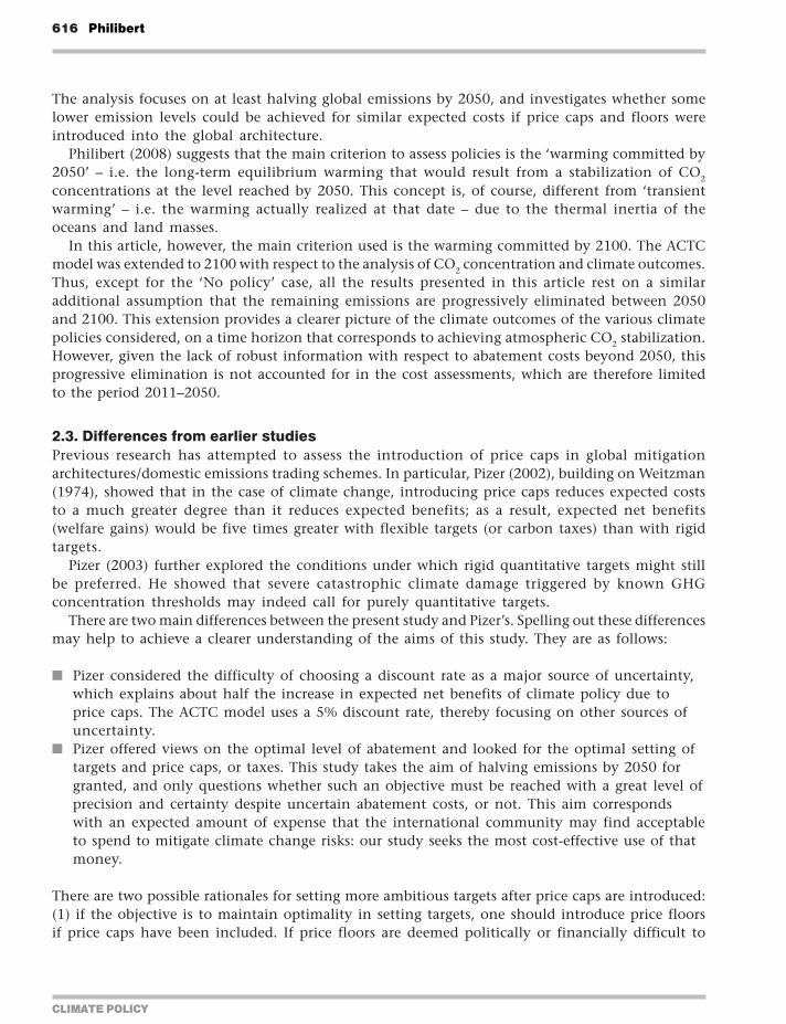
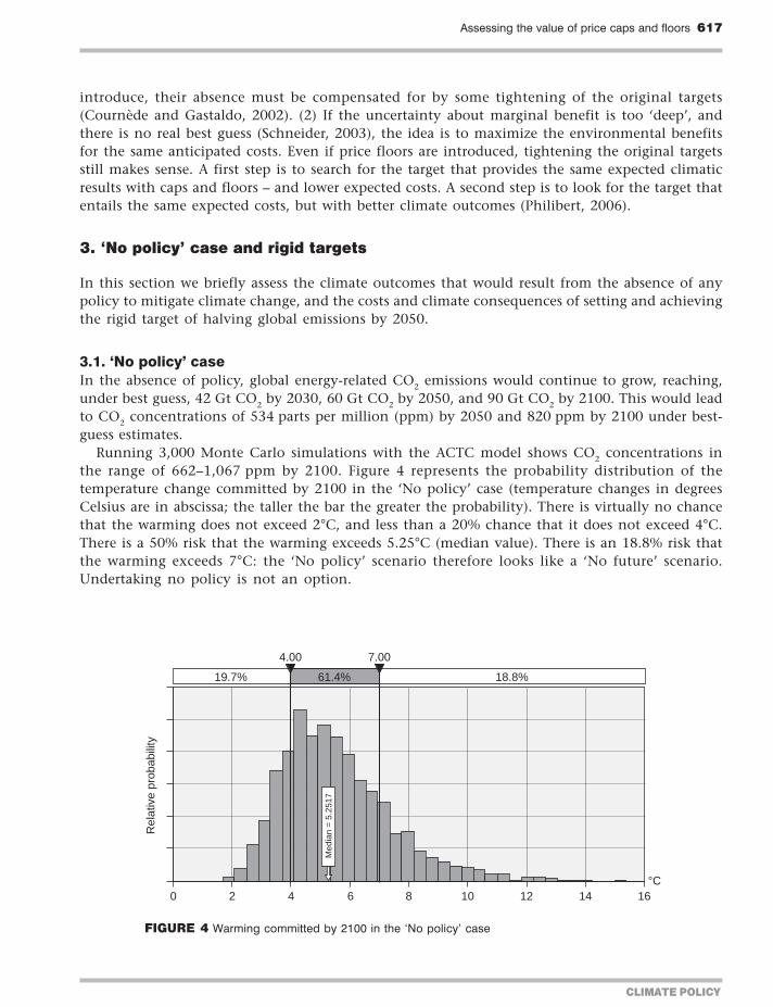
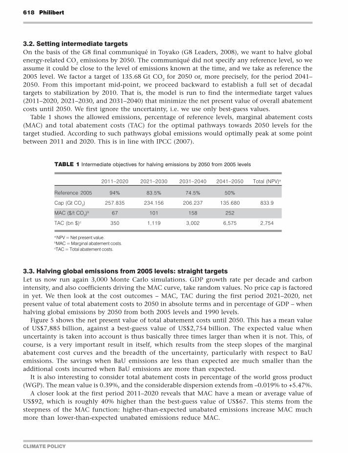
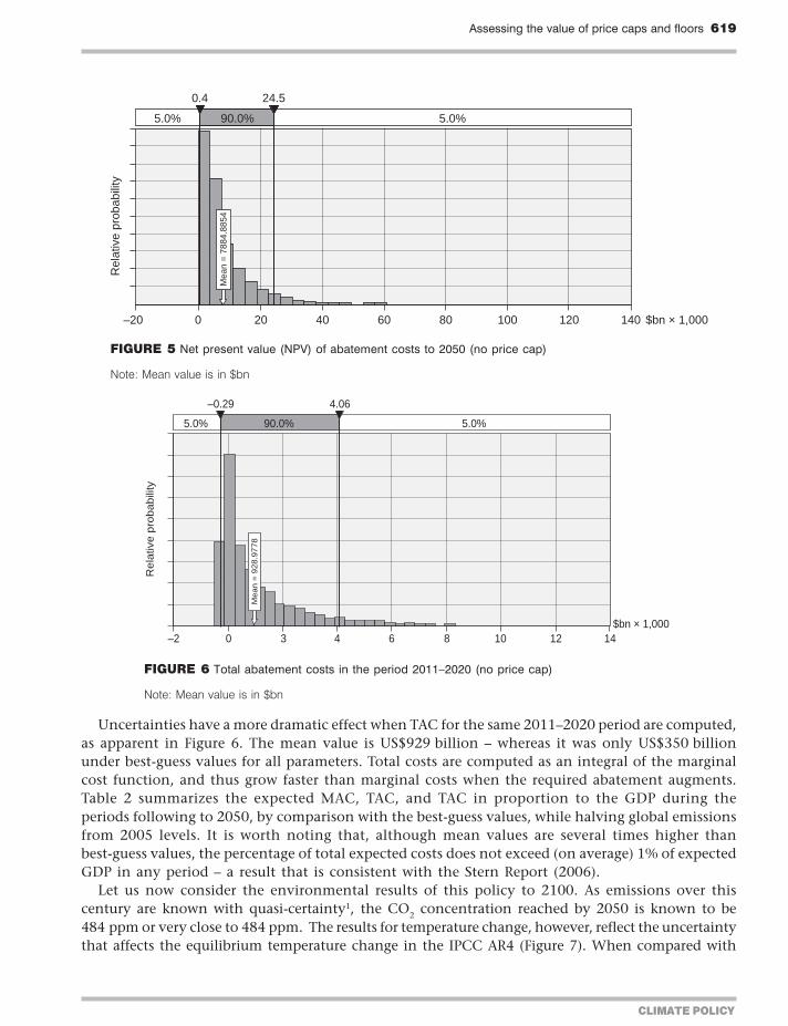
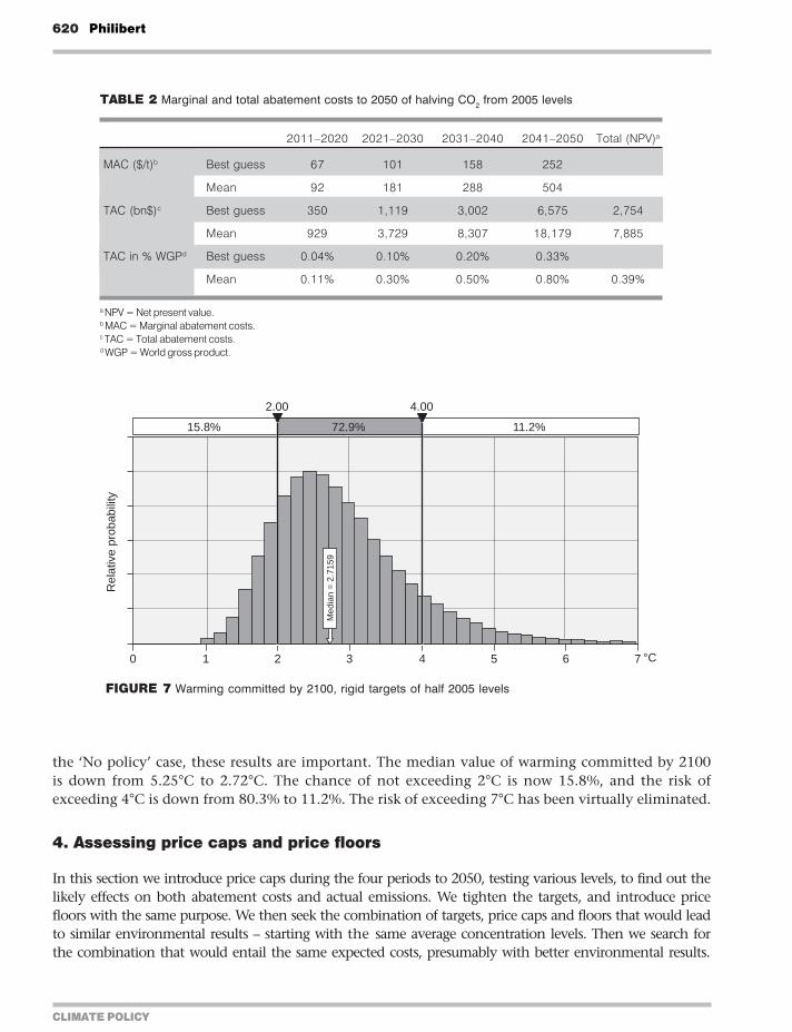
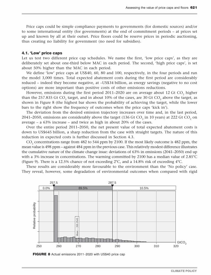
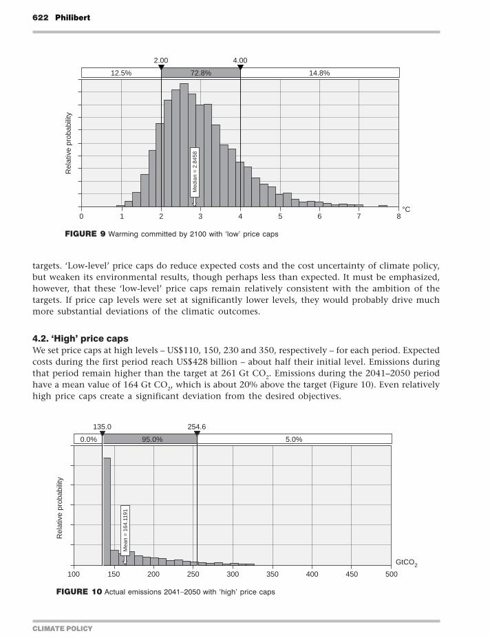
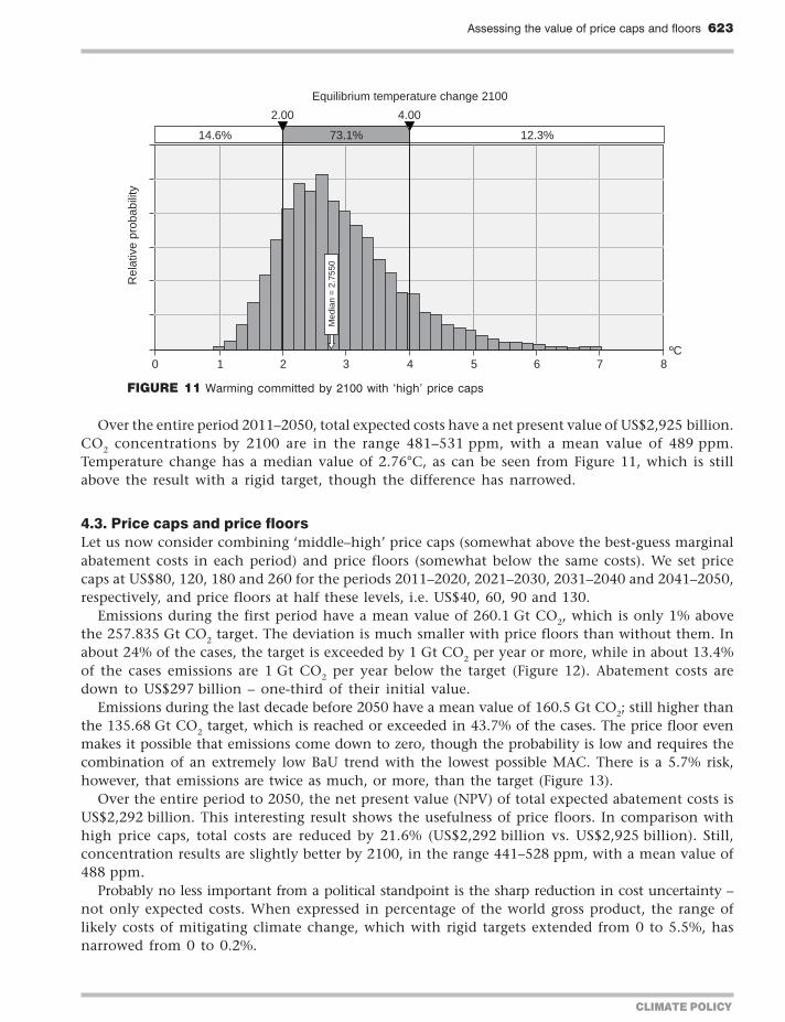
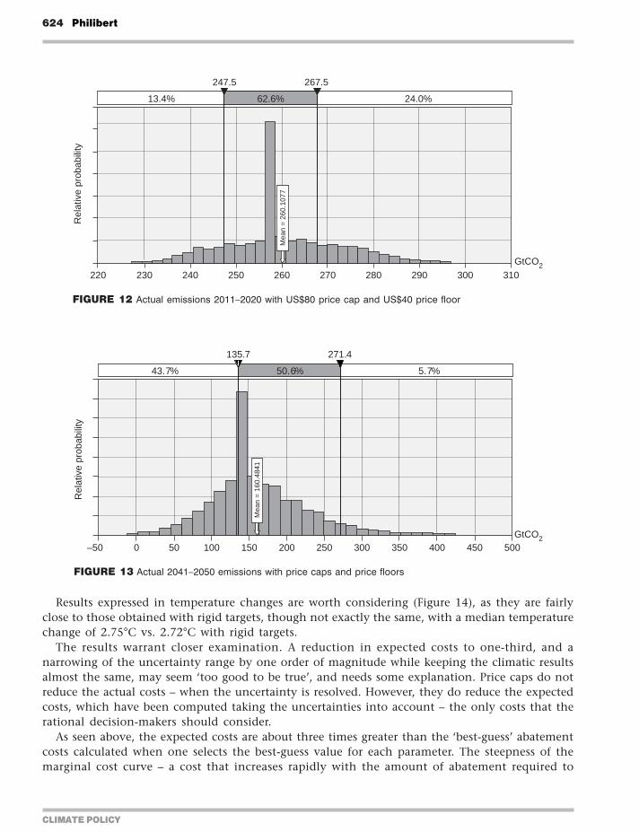
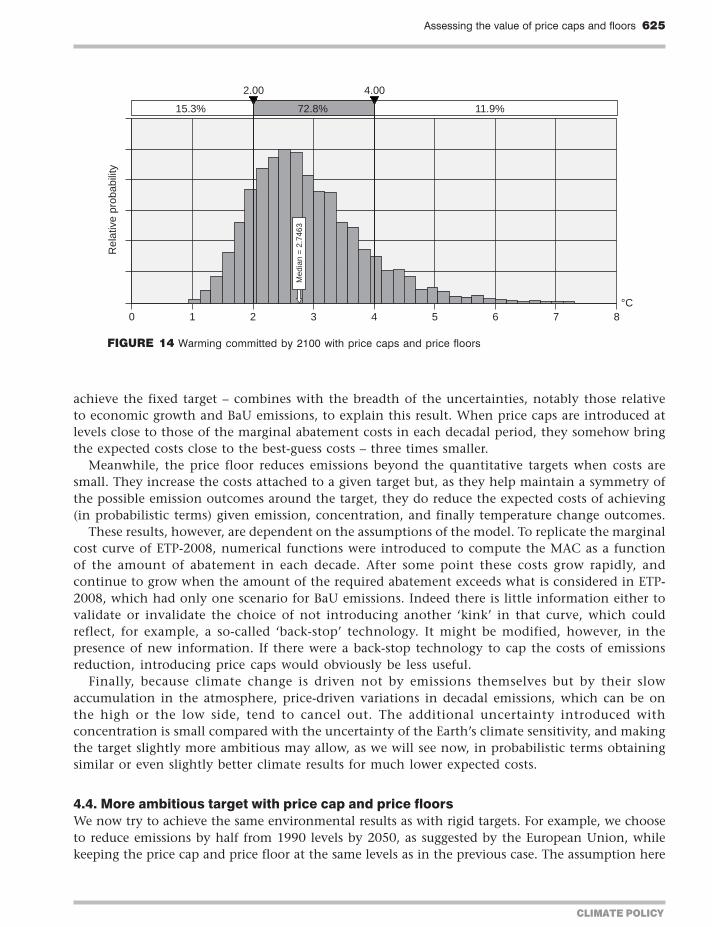
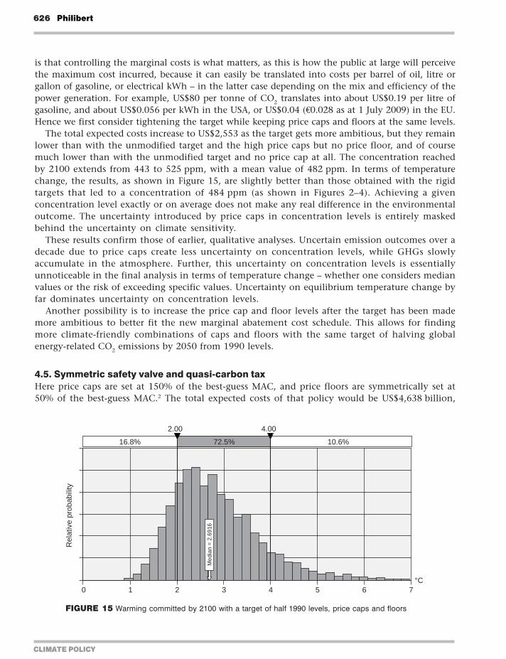
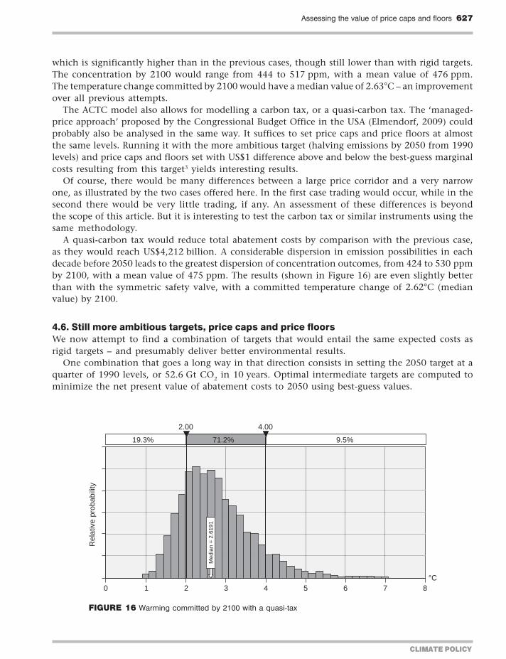
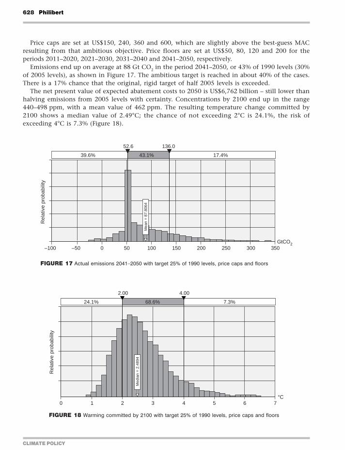
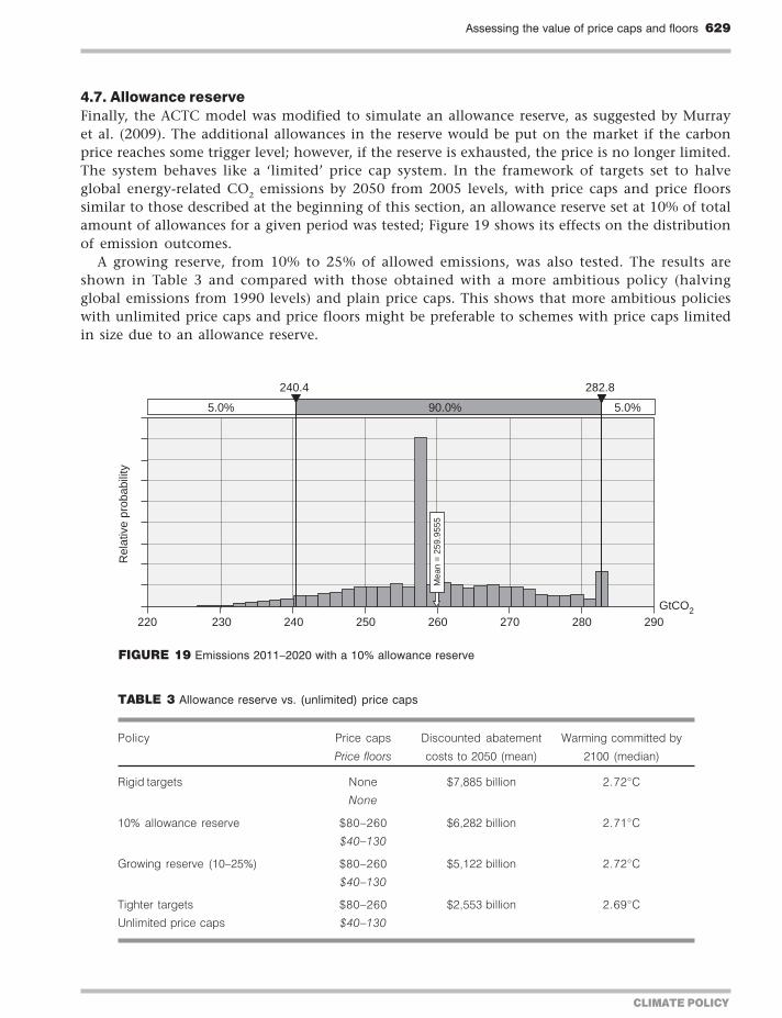
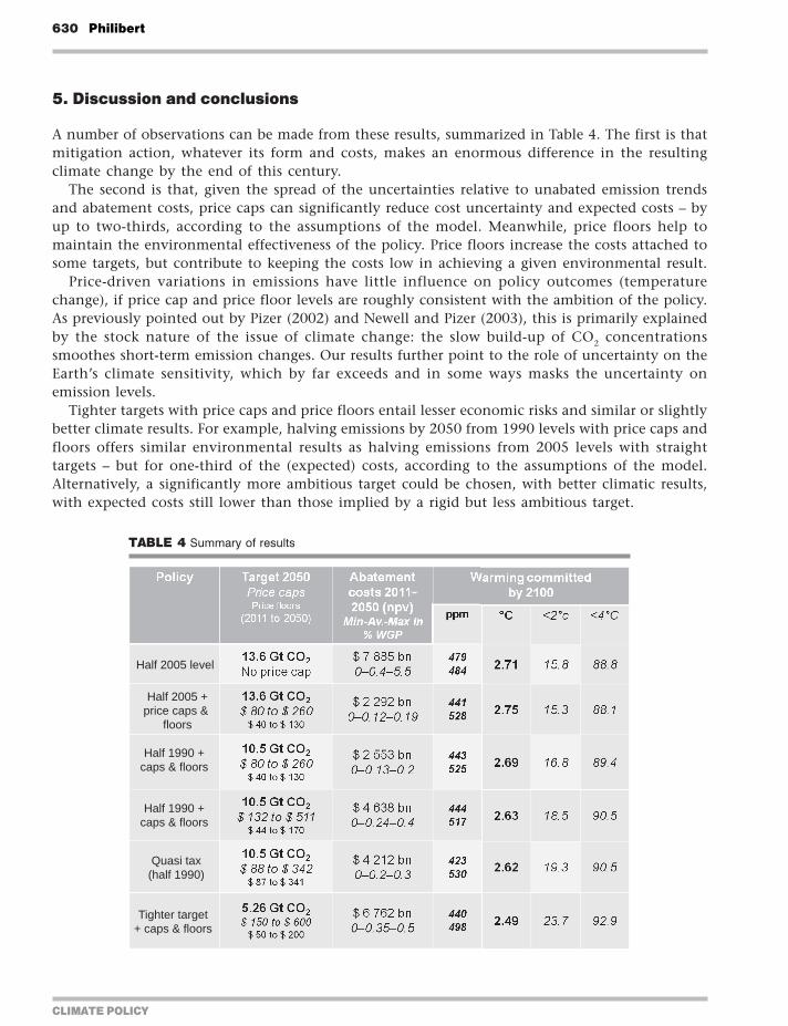
CLIMATE POLICY

632 Philibert

linking these schemes altogether when price caps and price floors are involved These issues requirefurther work

Acknowledgements

The views expressed here are those of the author and do not necessarily represent those of theIEA the OECD or their Member States I would like to express my gratitude to those whocontributed to this research in 2009 with their support comments criticisms or suggestions inparticular Paolo Frankl Brice Lalonde Claude Mandil Larry Goulder John Weyant MartyWeitzman Rob Stavins Charles Graves Metin Celebi Gregory Nemet Jake Jacoby DennyEllerman Richard Newell Jonathan Wiener Brian Murray Terry Dinan Dick MorgensternDallas Burtraw Harrison Fell Sacha Golub Nat Keohane Cathleen Kelly Richard Lorch andthree anonymous referees

Notes

1 There is a small probability that BaU emissions close to the end of the century could fall below target emissions asa result of the emission reductions undertaken in the early decades of the century but which because of how themodel is constructed permanently modify the BaU emission trajectory

2 The price caps would be set at US$132 per tonne CO2 in 2011ndash2020 US$202 in 2021ndash2030 US$318 in 2031ndash2040and US$511 in 2041ndash2050 Price floors would be set at US$44 in 2011ndash2020 US$67 in 2021ndash2030 US$106 in 2031ndash2040 and US$170 in 2041ndash2050

3 In this case price caps and floors would respectively be set at US$88 and 87 in 2011ndash2020 US$135 and 134 in 2021ndash2030 US$213 and 212 in 2031ndash2040 and US$342 and 341 in 2041ndash2050

References

Burtraw D Palmer K Kahn D 2009 A Symmetric Safety Valve Resources for the Future Washington DC [availableat wwwrfforgNewsFeaturesPagesA_Symmetric_Safety_Valveaspx]

Cournegravede B Gastaldo S 2002 lsquoCombinaison des instruments prix et quantiteacutes dans le cas de lrsquoeffet de serrersquoEacuteconomie et Preacutevision 156 2002ndash2005

Elmendorf DW 2009 Flexibility in the Timing of Emission Reductions Under a Cap-and-Trade Program Testimony beforethe Committee of Ways and Means US House of Representatives Congressional Budget Office [available atwwwcbogovdoccfmindex=10020]

Fell H Morgenstern RD 2009 Alternative Approaches to Cost-Containment in a Cap-and-Trade System Resources forthe Future Washington DC [available at wwwrfforgPublicationsPagesPublicationDetailsaspxPublicationID=20779]

Fell H McKenzie IA Pizer WA 2008 Prices versus Quantities versus Bankable Quantities Resources for the FutureWashington DC [available at wwwrfforgPublicationsPagesPublicationDetailsaspxPublicationID=20557]

G8 Leaders 2008 G8 Hokkaido Toyako Summit Leadersrsquo Declaration [available at wwwmofagojppolicyeconomysummit2008docdoc080714_enhtml]

Golub A 2009 Price Caps and Price Floors in Climate Policy Comments Presentation at the Center for Energy MarineTransportation and Public Policy Columbia University New York

IEA 2008 Energy Technology Perspectives Scenarios and Strategies to 2050 IEA ParisIPCC (Intergovernmental Panel on Climate Change) 2007 Fourth Assessment Report Synthesis Report GenevaKeohane NO 2009 lsquoCap and trade rehabilitated using tradable permits to control US greenhouse gasesrsquo Review of

Environmental Economics and Policy 3(1) 42ndash62Murray BC Newell RG Pizer WA 2009 lsquoBalancing Cost and Emissions Certainty An Allowance Reserve for Cap-

and-Tradersquo Review of Environmental Economics and Policy 3(1) 84ndash103

Assessing the value of price caps and floors 633

CLIMATE POLICY

Newell RG Pizer WA 2003 lsquoRegulating stock externalities under uncertaintyrsquo Journal of Environmental Economicsand Management 45 416ndash432

Philibert C 2006 Certainty versus Ambition Economic Efficiency in Mitigating Climate Change LTO Working Paper Series03 IEA Paris

Philibert C 2008 Price Caps and Price Floors in Climate Policy A Quantitative Assessment IEA Information Paper IEAOECD Paris [available at wwwieaorgtextbasepapers2008price_caps_floors_webpdf]

Philibert C Pershing J 2002 Beyond Kyoto Energy Dynamics and Climate Stabilisation IEAOECD ParisPizer WA 2002 lsquoCombining price and quantity control to mitigate global climate changersquo Journal of Public Economics

85 409ndash434Pizer WA 2003 Climate Change Catastrophes Discussion Paper 03-31 Resources for the Future Washington DCSchneider SH 2003 US Senate Committee on Commerce Science and Transportation Hearing on lsquoThe Case for Climate

Change Actionrsquo Center for Environmental Science and Policy Stanford University Stanford CAStern N 2006 Stern Review on the Economics of Climate Change HM Treasury LondonWeitzman ML 1974 lsquoPrices vs quantitiesrsquo Review of Economic Studies 41 477ndash491