Assessing the Impact of Nonperforming Loans on Economic ... · npls on economic growth over time...

371A. Jordan, C. Tucker Monetaria, July-December, 2013

Alwyn Jordan Carisma Tucker

Assessing the Impact of Nonperforming Loans

on Economic Growth in The Bahamas

Abstract

This paper examines the extent to which economic output and other variables affect nonperforming loans in The Bahamas utilizing a vec-tor error correction (vec) model. It also seeks to determine if there is a feedback response from nonperforming loans to economic growth. Data utilized in the study spanned the period September 2002 to De-cember 2011. The main findings reveal that growth in economic activ-ity tends to lead to a reduction in nonperforming loans, and there is additionally a small but significant feedback effect from nonperform-ing loans to output.

Keywords: nonperforming loans; Chow-Lin procedure; impulse-response functions.

jel Classification: G21

Senior Economist and Senior Research Assistant, respectively, at the Central Bank of The Bahamas. The views expressed in this paper are those of the authors and do not necessarily represent The Central Bank of The Bahamas. Email addresses: <[email protected]> and <[email protected]>.

372 Monetaria, July-December, 2013

1. INTRODUCTION

Since the start of the global economic recession in late 2007, commercial banks’ credit quality indicators in the Caribbean have deteriorated significantly, due to the rise

in unemployment rates, challenging business conditions and to some extent the significant increase in credit by consumers to support their expenditures prior to the recession.

The challenges faced by The Bahamas and the rest of the Caribbean are by no means unique; however, the rapid rise in nonperforming loans (npls), which have in some cases risen from around 5% of total loans in 2008 to over 10% by the end of 2011, based on imf estimates,1 are amongst some of the highest in the world. As The Bahamas continues to re-cover from recession, it is therefore prudent to attempt to de-termine the potential impact of elevated levels of arrears and npls on economic growth over time and whether there exist a feedback effect, as strong evidence of a negative relation could result in lower levels of growth going forward and increased vulnerabilities to external shocks. This has implications for economic policy making and forecasting. Based on studies, such as Espinoza and Prasad (2010) and Klein (2013), we ex-pect that there is a negative relation between gross domestic product (gdp) and npls.

This paper therefore seeks to determine, not simply the ex-tent to which economic activity and other variables affects npls in The Bahamas, but if there is also a feedback response from npls to economic growth, using an econometric framework. To the authors’ knowledge, this is the first of this type of study conducted for The Bahamas.

The remainder of the paper is organized as follows: Section 2 reviews the literature relating to the factors, which either af-fect or are impacted by the rise in npls in the banking sector. Section 3 provides a review of trends in arrears and npls for The Bahamas since 2002. Section 4 presents the econometric

1 See imf’s Regional Economic Outlook, “Western Hemisphere: Rebuil-ding Strength and Flexibility,” April 2012, p. 26.

373A. Jordan, C. Tucker

models utilized in the study and analyses the results and Sec-tion 5 concludes the study.

2. LITERATURE REVIEW

Over the past decade, there have been several papers produced which have tried to determine the causes of npls, especially as it relates to bank specific factors. There have also been studies that attempt to determine the relation between npls and other macroeconomic variables such as economic growth, and the extent to which npls affect real gdp.

Amador, Gómez-González, and Pabón (2013) studied the re-lation between abnormal loan growth and banks’ risk taking behavior, using information on individual Colombian banks’ balance sheets between June 1990 and March 2011. They used data from sixty-four financial institutions, provided by Colom-bia’s Financial Superintendence and they tested the abnormal loan growth on banks’ survival probability using information on individual banks’ characteristics during the financial crisis of the late 1990s. In addition, they tested the effect of abnormal loan growth on banks’ financial health (solvency, nonperform-ing loans and profitability), using cross-sectional time-series data on Colombian financial institutions between 1990 and 2011.

Their results show that abnormal loan growth during a sus-tained period led to reductions in banks’ capital ratios and to increases in the ratio of nonperforming loans to total loans. The authors also show that sustained abnormal loan growth was one of the most significant variables in explaining observed differences in the process of bank failure during the Colom-bian financial crisis of the late 1990s.

In their 2009 study, Khemraj and Pasha aimed to analyze the responsiveness of npls to macroeconomic and bank spe-cific factors in Guyana using regression analysis. They used a fixed effect panel model to ascertain the causes of npls in the Guyanese banking sector. As well, they utilized data from six commercial banks in Guyana over the period of 1994-2004, and estimated the model using pooled least squares. The


macroeconomic factors that were included in their model were: real gdp growth, inflation, and the real effective exchange rate. The bank specific factors used in this study were the real interest rate, bank size, annual growth in loans, and the ratio of loans to total assets. The results of their correlation analy-sis show that npls and the loans to assets ratio are positively related, implying that banks which take greater risks tend to have a greater amount of npls. The authors analysis also show that gdp growth and growth in npls are negatively related and that the size of the bank may not be relevant in terms of miti-gating credit risk, as larger banks did not have significantly lower npls. However, contrary to other studies, their results also indicated a “negative association between inflation and the ratio of npls to total loans”.

In a similar study, Espinoza and Prasad analyzed the extent to which macroeconomic factors affected npls of various banks within the Gulf Cooperative Council (gcc) countries and en-deavored to ascertain the causes of overall npls in the gcc banking sector. They used a dynamic panel of data retrieved from the database Bankwise™, and ran panel vector autore-gressive (var) models to determine the factors that affected the growth in npls in the gcc banking system. The authors tested bank specific factors2 as well as macroeconomic factors such as non-oil real gdp.

Their studies found that the npl ratio of the banks dete-riorated as interest rates rose and non-oil economic growth slowed, and the size of the banks played a role, as the larger banks as well as those with fewer expenses had less npls. They also found that a prior period of high credit growth could lead to increased npls in the future. In terms of the feedback ef-fects, the authors noted that there is a strong but short-lived feedback effect from npls to economic growth.

2 Bank specific factors tested were the capital adequacy ratio, the expenses/asset ratio, the cost/income ratio, the return on equity, size (of the banks), the lagged net interest margin, and lagged credit growth (deflated by the cpi).


Fofack (2005) also investigated npls in sub-Saharan Africa in the 1990s, and focused on determining if increases in npls were the major causes of bank failures. In his paper, the author utilized a standard definition of npls across the various coun-tries within the Communauté Financière Africaine (cfa)3 and non-cfa countries separately and compared the two sets of re-sults.4 His research revealed that financial costs were higher in non-cfa countries, as cfa costs fell over the 1996-2002 pe-riod, after the devaluation of the franc. He also examined the determinants of npls using correlation and causality analysis with a number of macroeconomic variables such as gdp per capita, inflation, interest rates, changes in the real exchange rate, interest rate spread and broad money supply (m2); as well as bank specific factors, such as return on assets and equity, net interest margins and net income, and interbank loans. The results of this analysis illustrate that real exchange rate appre-ciation and npls are positively related; however, the relation is not clearly defined for the non-cfa countries.

Fofack then conducted a Granger test to determine which, if any variables used in his study led to increases in npls. He used a sample of regional countries and found that inflation, real interest rates, and gdp growth per capita Granger cause npls in most of the countries. However, his study also found that in some countries the level of inflation and interest rates were not significant determinants of npls, and in those coun-tries, the Granger test revealed dual causality between gdp growth and rising npls. The author used a pseudo panel re-gression model to predict the potential impact that changes in banking sector variables and macroeconomic factors might

3 The cfa region comprises countries in the West African Economic and Monetary Union as well as countries in the Economic and Monetary Community of Central Africa. Although, the currencies are different in both regions.

4 The cfa franc is under a fixed exchange rate regime, formerly pegged to the French franc (now to the euro) and guaranteed by the French Treasury.


have on the banking sector.5 The results of the model show that gdp per capita, real interest rates, broad money supply (m2) and changes in real effective exchange rate were significant for the entire panel of countries, while other macroeconomic and bank specific variables were significant for a subset of the coun-tries. In terms of bank stability, growth in npls was found to be a major cause of bank failures due to their high costs and the banks’ lack of capital to withstand the effects of higher npls.

Dash and Kabras’ (2010) study aimed at determining the causes of npls in India using regression analysis. The macro-economic factors used in the model were the growth in real gdp, annual inflation, and the real effective exchange rate, as well as bank specific variables, including the real interest rate, bank size, annual growth in loans and the ratio of loans to total assets. Using a panel data set consisting of firm level data for six commercial banks operating through 1998-2008, the authors performed a correlation analysis which showed a strong negative relation between npls and real gdp growth, as well as a strong positive relation between npls and the loan to asset ratio. It also showed the ratio between npls and real interest rates and npls to total loans to be weak.

The results of their fixed effect regression model revealed that banks which take more risks are likely to have higher npls, the size of the bank is not important as a determinant of npls, and gdp growth is negatively related to npls. Their studies also indicated a negative relation between credit growth and npls, contrary to other literature, and their results showed mixed results between inflation and npls. Further, the real effective exchange rate exhibited a strong positive relation with npls, and loan delinquencies were higher for banks, which increase their real interest rates.

5 The variables used were: equity (% of total assets), return on assets, net interest, net income (% of total revenue), interbank loans (% of assets), equity (% of liquid assets), growth rate of real gdp, m2 (% of m2), inflation, domestic credit provided by banks (% of gdp), domestic credit to the private sector (% of gdp), real interest rate, change in real effective exchange rate, and gdp per capita.


De Bock and Demyanets (2012) focused on examining how credit growth and asset quality in emerging markets (ems) are affected by both domestic and external factors. The authors used variables that could possibly influence banks’ asset quality indicators, such as gdp growth, terms of trade, the exchange rate, capital flows, equity prices, and interest rates. Using a combination of dynamic panel and structural panel var mod-els for 25 ems during the 1996-2010 period, the authors ana-lyzed the effects on the real economy when credit contracts or banks’ balance sheets deteriorate.

The results of their dynamic panel regressions show that im-portant determinants of loan quality are portfolio and bank flows, economic growth, terms of trade, and exchange rate appreciation, which all are negatively related with the aggre-gate npl ratio, while credit growth was found to be positively related with the npl ratio, contrary to previous studies. The re-sults of their structural panel var show that worsening growth prospects, a depreciating exchange rate, weaker terms of trade and a decrease in debt-creating capital inflows will potentially decrease private sector credit and worsen banks’ asset quality indicators. Moreover, the authors also found that an increase in npls leads to less economic activity and that credit contracts when the exchange rate tends to depreciate.

Badar and Javid (2013) carried out a study with the purpose of examining the long run relation between macroeconomic variables and npls; examining the short run impact of macro-economic forces on npls; and facilitating monetary and fiscal regulators to cover up the gaps and to make right decisions by sharing empirical results of the study. The authors used five macroeconomic variables in their study to examine the im-pact on npls: inflation, interest rate, gross domestic product, exchange rate and money supply. They carried out a bivariate and multivariate cointegration analysis, as well as a Granger causality test, before carrying out a vector error correction (vec) model. Their results showed that a long run relation be-tween macroeconomic forces and nonperforming loans exists, and the Johansen multivariate cointegration test confirmed


it; similarly, the bivariate cointegration confirms a long run relation exists between nonperforming loans with money sup-ply and interest rates. Weak short run dynamics were found between npls, inflation and exchange rate by the vec model.

Similarly, Klein aimed to evaluate the determinants of npls in Central, Eastern and South Eastern Europe (cesee) econo-mies by looking at both bank-level data and macroeconomic indicators over 1998-2011. The author also aimed to evaluate the feedback effects from the banking sector to the real econ-omy through a panel var analysis in order to assess how the recent increase in npls in the cesee region is likely to affect economic activity in the period ahead. The panel var includ-ed five variables: npls, real gdp growth, unemployment rate, the change in credit-to-gdp ratio and inflation.

The author’s results confirmed that the level of npls tends to increase when unemployment rises, exchange rate depreci-ates, and inflation is high. The results also suggest that higher euro area’s gdp growth results in lower npls. As it relates to bank-level factors, the author found that higher quality of the bank’s management, as measured by the previous period’s profitability, leads to lower npls, while moral hazard incen-tives, such as low equity, tend to worsen npls. In addition, ex-cessive risk taking (measured by loans-to-assets ratio and the growth rate of bank’s loans) was found to contribute to higher npls in the subsequent periods.

While examining the feedback effects between the banking system and economic activity the author found that npls were responsive to macroeconomic conditions, such as gdp growth, and that there are feedback effects from the banking system to the real economy. To be specific, Klein’s estimations suggest that an increase in npls has a significant impact on credit (as a share of gdp), real gdp growth, unemployment, and infla-tion in the periods ahead.

3. ANALYSIS OF ARREARS

For the purpose of the study, we utilized quarterly data for The


Bahamas, which spanned the period September 2002 –the ear-liest date at which a consistent quarterly asset quality series is available– until March 2012.

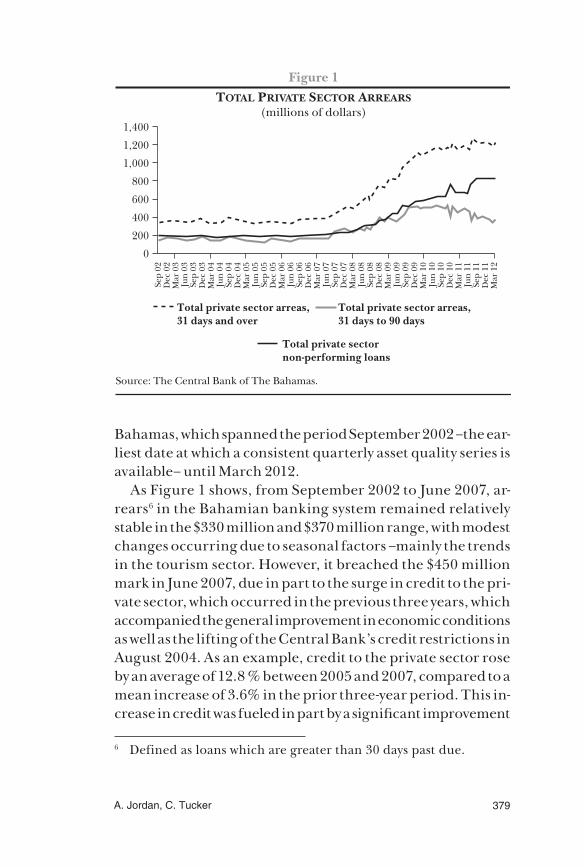
As Figure 1 shows, from September 2002 to June 2007, ar-rears6 in the Bahamian banking system remained relatively stable in the $330 million and $370 million range, with modest changes occurring due to seasonal factors –mainly the trends in the tourism sector. However, it breached the $450 million mark in June 2007, due in part to the surge in credit to the pri-vate sector, which occurred in the previous three years, which accompanied the general improvement in economic conditions as well as the lifting of the Central Bank’s credit restrictions in August 2004. As an example, credit to the private sector rose by an average of 12.8 % between 2005 and 2007, compared to a mean increase of 3.6% in the prior three-year period. This in-crease in credit was fueled in part by a significant improvement

6 Defined as loans which are greater than 30 days past due.

Source: The Central Bank of The Bahamas.

Figure 1TOTAL PRIVATE SECTOR ARREARS

(millions of dollars)

Sep

02D

ec 0

2M

ar 0

3Ju

n 03

Sep

03D

ec 0

3M

ar 0

4Ju

n 04

Sep

04D

ec 0

4M

ar 0

5Ju

n 05

Sep

05D

ec 0

5M

ar 0

6Ju

n 06

Sep

06D

ec 0

6M

ar 0

7Ju

n 07

Sep

07D

ec 0

7M

ar 0

8Ju

n 08

Sep

08D

ec 0

8M

ar 0

9Ju

n 09

Sep

09D

ec 0

9M

ar 1

0Ju

n 10

Sep

10D

ec 1

0M

ar 1

1Ju

n 11

Sep

11D

ec 1

1M

ar 1

2

1,400

1,200

1,000

800

600

400

200

0

Total private sector arreas, 31 days and over

Total private sector arreas, 31 days to 90 days

Total private sector non-performing loans


in business conditions, as economic output rose by an average of 2.5% over the three-year period, due to growth in the tour-ism sector and projects such as Atlantis Phase III. In addition, employment conditions improved, as the jobless rate averaged 8.6% between 2005 and 2007, vis-à-vis 10.0% in the prior three years, which allowed more customers to qualify for various types of loans from these lending institutions.

Between June 2007 and December 2009, arrears climbed steadily, reflecting the rapid deterioration of economic and employment conditions –particularly in the tourism and for-eign investment sectors–, which resulted from the global finan-cial crisis and subsequent recession. The Bahamas’ real gdp growth slowed from 2.5% in 2006 to 1.4% in 2007, and fell by 2.3% in 2008 and 4.9% in 2009.7 Additionally, the unemploy-ment rate almost doubled from 7.6% in 2006 to 14.2% by 2009. As a result, a significant number of borrowers were unable to meet their debt payments, due to the fact that they were either laid off or worked reduced hours –as occurred in the lodging sector– and in the case of firms, there was a significant contrac-tion in their revenues, due to reduced business activity.8 There-fore, from 2007 to 2009, arrears rose by an average of 40% per annum, despite banks’ attempts to engage in various types of debt restructuring programs.

Over the 2010 to 11 period, the rate of growth in arrears slowed considerably to 5.3%, as economic conditions appeared to stabilize, with real gdp rising marginally by 0.2% in 2010 and by 1.1% in 2011; however, the level of output remained sig-nificantly below the pre-recession period.9

7 Based on estimates from the Bahamas Department of Statistics as at end-April 2012.

8 There is also some anecdotal evidence to suggest that some consu-mers were also adversely affected, because they had obtained other forms of credit in addition to the facilities offered by commercial banks; however, comprehensive information on non-bank lending and arrears is not readily available.

9 Table 1 (Appendix A) provides details on some of the key credit quality indications in the banking system from 2002 to 2011.


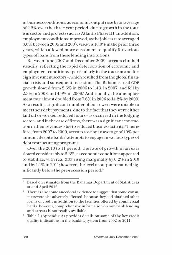
A disaggregation of arrears by average age revealed major increases in both the short term (loans 31 to 90 days in arrears) and the npl segment (91 days and over). Trends in the short-term category tended to follow changes in total arrears over the 2002 to 2009 period, however, since December 2009, short-term arrears have trended downwards, as npls have driven the increase in arrears over the two-year period.

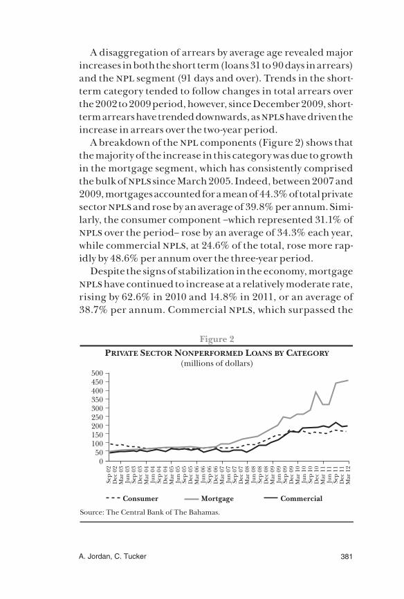
A breakdown of the npl components (Figure 2) shows that the majority of the increase in this category was due to growth in the mortgage segment, which has consistently comprised the bulk of npls since March 2005. Indeed, between 2007 and 2009, mortgages accounted for a mean of 44.3% of total private sector npls and rose by an average of 39.8% per annum. Simi-larly, the consumer component –which represented 31.1% of npls over the period– rose by an average of 34.3% each year, while commercial npls, at 24.6% of the total, rose more rap-idly by 48.6% per annum over the three-year period.

Despite the signs of stabilization in the economy, mortgage npls have continued to increase at a relatively moderate rate, rising by 62.6% in 2010 and 14.8% in 2011, or an average of 38.7% per annum. Commercial npls, which surpassed the

Source: The Central Bank of The Bahamas.

Figure 2PRIVATE SECTOR NONPERFORMED LOANS BY CATEGORY


Sep

02D

ec 0

2M

ar 0

3Ju

n 03

Sep

03D

ec 0

3M

ar 0

4Ju

n 04

Sep

04D

ec 0

4M

ar 0

5Ju

n 05

Sep

05D

ec 0

5M

ar 0

6Ju

n 06

Sep

06D

ec 0

6M

ar 0

7Ju

n 07

Sep

07D

ec 0

7M

ar 0

8Ju

n 08

Sep

08D

ec 0

8M

ar 0

9Ju

n 09

Sep

09D

ec 0

9M

ar 1

0Ju

n 10

Sep

10D

ec 1

0M

ar 1

1Ju

n 11

Sep

11D

ec 1

1M

ar 1

2

500450400350300250200150100

500

Consumer Mortgage Commercial


consumer segment to become the second largest category in June 2010, recorded a slowdown in the rate of growth to 11.3% over the two-year period, while the consumer segment fell by an average of 1.9%. Over the review period, mortgage npls accounted for almost half (49.5%) of the total, followed by the commercial and consumer segments with shares of 27.3% and 23.2%, respectively.

4. ECONOMETRIC ANALYSIS

4.1 Data

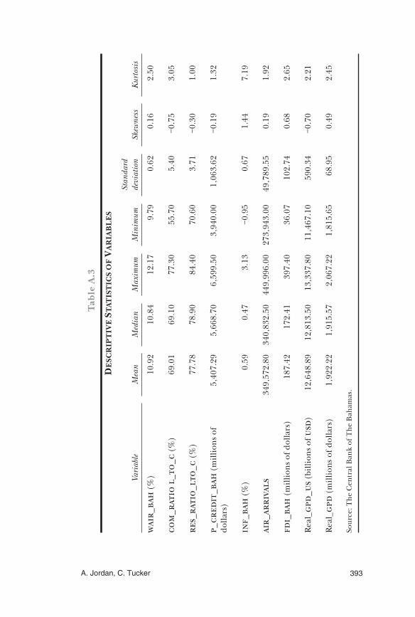
In order to investigate the effect which economic growth has on nonperforming loans in The Bahamas, the factors that in-fluence nonperforming loans must first be determined. In this initial step, we used several macroeconomic variables in the model, which served as indicators of economic activity and in-terest rates in the country. Variables included were:10 real gdp in The Bahamas (real_gpd); United States real gdp (real_gpd _us); air arrivals (air_arrivals), which served as a proxy for tourism sector output;11 foreign direct investment (fdi); the weighted average loan rate (wair _bah); and inflation (inf _bah). Addi-tionally, we used credit to the private sector (p _credit) to rep-resent consumer demand (Table A.2, Appendix A, shows all of the variables and the expended sign of their coefficients). The dependent variable used in the regression analysis was total private sector npls (p _npl).12 The quarterly data was ob-tained from various sources including: The Central Bank of The Bahamas’ Quarterly Statistical Digest and unpublished da-tabases, while the information for United States real gdp was

10 Based on the work of Khemraj and Pasha (2009), Espinoza and Prasad (2010), and Fofack (2005).

11 Since the majority of the high value-added stopover tourists are air visitors, it seemed prudent to use this indicator as a proxy for tourism output.

12 All of the variables are in nominal terms with the exception of the real gdp variables.


obtained from the Bureau of Economic Analysis.13 The time-frame was limited to 2002Q3 to 2011Q4, because data on com-mercial banks’ credit quality indicators was only compiled on a consistent aggregate basis from 2002. Table A.3 (Appendix A) provides some descriptive statistics for the variables used in the model.

4.2 Results: Real gdp

The real gdp series (real_gpd) for The Bahamas presented a significant challenge, since this indicator is only compiled on an annual basis. However, for the purpose of the model, a quarterly real gdp series needed to be obtained to employ the econometric techniques required, since annual data would have significantly diminished the validity of any statistical tests conducted, due to the low level of the degrees of free-dom14 and limited the ability to create var models. In order to disaggregate the annual real_gpd series, the variables which were important in affecting real_gpd over time and for which quarterly data was available, needed to be determined initial-ly. In the context of The Bahamas, where tourism and foreign direct investment are two of the main drivers of economic ac-tivity, the variables air arrivals (air_arrivals) and foreign direct investment (fdi _bah) were used in the model. Credit to the private sector (p _credit _bah) was also included in the model given its close correlation with consumption.15 The final vari-able selected was real gdp in the United States (real _gpd _us), given the fact that the country is historically The Bahamas’ major trading partner, accounting for the majority of visitor arrivals, imports and foreign investment. The regression was conducted using the ordinary least squares (ols) technique

13 See website: <www.bea.gov>.14 That is, in a model with n observations and k variables, there exists

n−k degrees of freedom. 15 Based on the expenditure approach, private consumption accoun-

ted for an estimated 61% of output in 2011.


and the results for the best model, based on the reported sta-tistics, are shown in equation 1.

1 (8.930073) (2.694389)

( 3.262680)

_ 0.681014 _ _ 0.001131

0.771236 _

real GDP real GDP US air_arrivals

FDI BAH−

= + −

−

2 20.943641 0.928271 1.703817R R DW= = =

Note: t-statistic values are in parenthesis. All are significant at 5% level.

All of the variables had the a priori signs, with the excep-tion of fdi _ bah. Further analysis of the negative value for the fdi _ bah coefficient, led to the theory that due to the high correlation between fdi and imports (almost 90%) an increase in fdi would initially retard growth due to its positive effect on imports and hence negative impact on gpd.16 As the R2 and

2R values show, the model is a very good fit for real _gpd over the period 1997 to 2011,17 accounting for 94.3% and 92.8%, re-spectively, of the movement in the real _gpd series.

The next step involved disaggregating the annual real _gpd series into quarterly data, utilizing the Chow and Lin (1971) procedure. This technique was chosen based on the work con-ducted by Abeysinghe and Lee (1998), who noted that disag-gregated gdp series based on the Chow-Lin (c-l) procedure produced superior estimates when compared to series, which were generated solely from univariate techniques.

According to Abeysinghe and Rajaguru (2004), the meth-odology used stems from the procedure developed by Chow and Lin (1971). The basic idea is to find gdp-related quarterly series and determine a predictive equation by running a re-gression of annual gdp on annual values of the related series.

16 These results were also found to be insensitive to lagged values for fdi.

17 The real gdp series for 1997 to 2011 was obtained from the De-partment of Statistics and is based on the latest estimates, which were rebased in 2010.


The quarterly figures of the related series were then utilized to predict the quarterly gdp figures.18

The econometric software package rats® was employed to generate the results based on the c-l procedure.19 For the pur-pose of this exercise, we used specific settings, based inter alia on the assumption that a linear relation exists between the vari-ables and that the quarterly real gdp series sum to the annual values. Following the work of Frain (2004), we used a value of p that was sufficiently large to ensure that the estimate con-verges, in this case 0.95%. Since the procedure disaggregated the data to ensure that real gdp summed to the annual gdp series, and seasonal factors such as changes in tourism sector output also impacted the estimates, quarterly changes in real gdp were estimated based on the formula shown in Equation 2:

2 4

4

_ __ 100

_qt qt

qtqt

real GDP real GDPreal GDP

real GDP−

−

−∆ = ×

According to the quarterly estimates,20 the Bahamian econ-omy has experienced three recessions21 since 1997, with the lat-est beginning in 2008Q3 and ending in 2009Q3 –this was also the longest and most severe recession based on the estimates.

4.3 Results: Nonperforming Loans

4.3.1 Long-run Results

To explore the effect of the explanatory variables on nonper-forming loans, the var methodology was employed. In the ini-tial step, we tested the variables for the order of integration,

18 See Appendix B for a derivation of the Chow Lin methodology.19 rats uses two procedures to disaggregate series into a higher

frequency, the Chow-Lin and Dissagregate procedures; however, given the parameters specified in the model, both techniques produced very similar results.

20 See Appendix A, Table A.3.21 Defined as two consecutive quarters of economic contraction.


i.e., whether or not they were stationary, using the Philips-Perron (pp) test. As expected all of the interest rate variables were integrated of order zero I(0), as well as inf _bah, air_ar-rivals _bah and fdi _bah, while the other variables were I(1). Due to the limited number of observations and large number of regressors, an ols model was first estimated and the signif-icant explanatory variables in the model were determined by the general to specific methodology. Variables which were not significant in the regression were dropped as noted by their p -values at the 5% level of significance. Equation 3 shows the results for the optimal model estimated.

3 (9.46589)*(4.217336)*

( 5.239256)*

2,060 0.162349 _

1.358177 _

P_NPL P_credit BAH

real GDP−

= + −

− .

2 20.748462 0.733666 0.520262.R R DW= = =

The variables which proved to be significant in the model were p _credit _bah, and real _gpd.22 The variables were then placed in a var framework and tests for cointegration con-ducted.23 Given that all of the variables in Equation 3 were I(1), the maximum number of cointegrating vectors can be k−1 where k is the number of variables in the model. Then, we conducted a Johansen cointegration test to determine the number of cointegrating vectors, optimal lag length and type of cointegrating equation, as determined by the Schwartz cri-teria. Table A.4 presents the results of the cointegration test (Appendix A). Sequential tests using different lag pairs were conducted and the test which produced the smallest value of the Schwartz information criterion (sic)24 was used to select

22 The results of the Durbin-Watson statistic show that there is first order serial correlation in the model; however this was eliminated when two lags of the dependent variable are included in the model.

23 See Verbeek (2000) for a detailed description of the vec methodo-logy.

24 Due to data constraints, only six lag pairs were tested.


the model specification, and number of cointegrating equa-tions. Based on the results of the test, a vector error correction (vec) model with one cointegrating equation, lag pairs 1 to 2, and model specification intercept and no trend was estimat-ed. Equation 4 shows the results for the long-run model. As ex-pected both the real _gpd and p _credit _bah variables had the correct sign. The coefficient of the real _gpd suggests a greater effect on p _npl from an increase than for p _credit _bah and both coefficients were significant at the 5% level.

4

( ) ( )

( )

1 1( 5.239256)(5.64314)

1(10.1763)

7,240.770 4.798655 _

0.477958 _ _

P_NPL real GDP

P credit BAH

− −−

−

= − +

+

4.3.2 Short-run Results

Table A.5 (Appendix A) shows that the short-run model which normalized on the p _npl variable had a valid error correction term (i.e., negative and significant), which showed that the cointegrating relation between the variables was valid. Then, we conducted a Granger causality/block exogeneity test to de-termine if the selected endogenous variables should be treated as exogenous and the results indicated that all of the variables should be treated as endogenous.25

In order to explore the short-run dynamics of the system, for each of the variables in the system26 we generate some general-ized impulse-response functions. These functions measure the time profile of the effects of shocks at a given point in time on the (expected) future values of variables in a dynamic system and are insensitive to the ordering of the variables in the system.

Based on the results for the accumulated responses over a three year (12 quarters) period (Figure A.2, Appendix C), an innovation or positive shock to real _gpd equal to one standard deviation, ceteris paribus, resulted in a persistent reduction

25 See Table 6 (Appendix A).26 See Pesaran and Shin (1998).


in the p _npl variable. Meanwhile, a shock of similar relative magnitude to p _npl has an almost identical effect on real _gpd. This result is not surprising for The Bahamas, given that over the period estimated, the growth in gdp was accompanied by increased levels of employment and most likely generally higher salaries, since a significant portion of the population receive salary increases when new union agreements are reached. This therefore provided greater scope for individuals to obtain and repay new loans, based on several criteria including their level of compensation. In addition, it is worth noting that a positive one standard deviation innovation to p _credit _bah resulted in an increase in p _npl over time; however, a positive shock to p _npl results in a decrease in p _credit _bah over time.

The analysis appears to suggest that there is a feedback rela-tion between the real _gpd and p _npl, or that output growth tends to reduce npls over time, and that increases in npls also appear to have a retarding effect on real gdp –the effects are rather small initially but increase rapidly over time. A positive shock of one standard deviation to quarterly output reduces npls by a mere $16 million in the first quarter; however, the ac-cumulated impact is approximately $76.5 million by the end of the first year and goes to over $400 million by the end of third year, or approximately 40% of npls at end-December 2011. Similarly, a one standard deviation innovation to npls reduces real gdp by only an estimated $24.9 million in the first quarter, and this rapidly increases to $93.2 million by the end of the first year and by the end of the third year, the value of the accumu-lated responses is $343.5 million, equivalent to 5% of 2011’s total gdp. In addition, one standard deviation positive inno-vation to private sector credit appears to have weaker positive effect on npls, resulting in an increase in npls of $5.2 million by the end of the first quarter and this rises to $33.7 million by the end of the first year and the accumulated responses reach $249.2 million by the end of the 12th quarter. In contrast, a one standard deviation increase in npls appears to have a negative effect on private sector credit, with the exception of the first period, when credit rises by $11.1 million, but then declines by


a total of $94.0 million after year one and by an accumulated response of $866.3 million by year three.

The results appear to be relatively robust, as the replace-ment of p _npl with ratio of npls to total private sector loans (p _npl _ratio), as the dependent variable, produced similar accumulated impulse response profile.27 In addition, with the exception of the positive relation between shocks to private sec-tor credit and npls, the results for the p _npl model are gen-erally consistent with those observed by other authors such as Nkasu (2011), and Espinoza and Prasad (2010). Note, for the former that an adverse shock to gdp growth for a panel of 26 advanced countries causes an increase in the ratio of npls to total loans, while an increase in npls tends to slow gdp growth. Moreover, Nkasu found a negative relation between npls and private sector credit, as defined by the ratio of private sector credit to gdp. Similarly, as reported in Section 2, Espinoza and Prasad noted that the high non-oil gdp growth reduced the ra-tio of npls to total loans for a model of six countries gcc coun-tries, while an increase in the npl ratio tended to reduce gdp growth. Further, the authors found that higher npls tended to reduce credit growth and vice versa.

5. CONCLUSION AND POLICY IMPLICATIONS

The paper analyzed the trends noted in commercial banks ar-rears and nonperforming loans over a ten year period based on quarterly data. It then provided an analysis of the impact of key economic indicators on non-accrual loans in the bank-ing system, to determine whether there was a feedback effect on economic growth from an increase in npls.

The tests show that based on the results of the regression, which conform to similar findings noted by other authors, growth in economic activity tends to lead to a reduction in npls in both the short- and long-run; however, there was also a feedback effect from npls to real gdp.

27 See Chart 5 (Appendix C).


From a policy perspective, the results imply that policy mak-ers should implement countercyclical policy measures, aimed at reducing the potential for a significant build up in npls dur-ing periods of economic downturn as this could slow the pace of a subsequent economic recovery over time. Further, the analy-sis suggests that the authorities could seek ways of restraining credit growth over the long-term, although the direct effects on npl from an expansion in this variable are weaker than those obtained from shocks to output in both the long- and short-run. Finally, the study indicates that economic growth in the economy could reduce npls over time and this most likely re-flects the effect of growth on employment and business condi-tions and hence borrowers’ ability to repay loans.

However, it is worth noting that the results are preliminary and the quarterly gdp series calculated serves only as a proxy to gdp obtained using more robust data collection methods. Finally, the span of the data series is still quite short at 10 years and only includes three recession periods, based on the results of the c-l disaggregation. A longer time series could assist in strengthening the results or reveal other important relations.

Appendices

Appendix A


Tabl

e A

.1

KE

Y C

RE

DIT

QU

AL

ITY

IND

ICAT

OR

S O

F T

HE

BA

HA

MIA

N B

AN

KIN

G S

YST

EM

, 200

2-20

11

20

0220

0320

0420

0520

0620

0720

0820

0920

1020

11

Tota

l pri

vate

sect

or a

rrea

rs (

mill

ions

of

dolla

rs)

356.

938

6.7

373.

337

0.2

394.

252

9.9

765.

81,

090.

11,

139.

11,

208.

1

As p

erce

ntag

e of

tota

l pri

vate

sect

or lo

ans

9.9

10.4

9.4

8.3

7.7

9.4

12.7

17.8

18.6

19.3

Tota

l pri

vate

sect

or a

rrea

rs (

31-9

0 da

ys)

(mill

ions

of d

olla

rs)

168.

518

9.3

176.

516

8.6

178.

127

8.2

398.

051

3.7

393.

239

2.0

As p

erce

ntag

e of

tota

l pri

vate

sect

or lo

ans

4.7

5.1

4.4

3.8

3.5

5.0

6.6

8.4

6.4

6.3

Tota

l pri

vate

sect

or n

onpe

rfor

min

g lo

ans

(mill

ions

of d

olla

rs)

188.

419

7.4

196.

820

1.6

216.

025

1.8

367.

857

6.4

745.

981

6.1

As p

erce

ntag

e of

tota

l pri

vate

sect

or lo

ans

5.2

5.3

5.0

4.5

4.2

4.5

6.1

9.4

12.2

13.0

Tota

l pro

visi

ons (

mill

ions

of d

olla

rs)

68.6

78.8

87.8

89.5

118.

212

0.7

169.

121

3.6

272.

729

9.6

As p

erce

ntag

e of

tota

l pri

vate

sect

or lo

ans

1.9

2.1

2.2

2.0

2.3

2.2

2.8

3.5

4.4

4.8

Deb

t con

solid

atio

n lo

ans (

mill

ions

of

dolla

rs)

350.

934

3.7

346.

841

3.2

459.

849

6.3

594.

664

8.0

714.

682

8.6

Perc

enta

ge o

f cha

nge

−2.1

0.9

19.1

11.3

7.9

19.8

9.0

10.3

16.0

Tota

l pri

vate

sect

or lo

ans (

mill

ions

of

dolla

rs)

3,59

7.0

3,72

3.1

3,96

9.6

4,46

6.3

5,14

0.8

5,61

0.6

6,01

2.6

6,10

9.9

6,13

2.6

6,26

6.7

Sour

ce: C

entr

al B

ank

of T

he B

aham

as.


Table A.2

VARIABLE NAMES AND EXPECTED SIGNSEndogenous variable: private sector nonperforming loans (p_npl)

Exogenous variables

Regressors

Expected

signs

Order of integration (pp test)1

Weighted average interest rate on loans and overdrafts

wair_bah + I(0)

Average loan value/cost ratio (commercial)

com_ratio l_to_c

+/− I(0)

Average loan value/cost ratio (residential)

res_ratio_lto_c

+/− I(0)

Credit to the private sector p_credit_bah + I(1)Inflation inf_bah + I(0)Air arrivals air_arrivals − I(0)Foreign direct investment fdi_bah − I(1)Real gdp us real_gpd_us − I(1)Real gdp Bahamas real_gpd − I(1)Private sector nonperforming loans

p_npl N/A I(1)

Source: The Central Bank of The Bahamas.1 Philips-Perron test, with significance at 5% level.

Source: Author’s calculations.

Figure A.1DISAGGREGATED REAL GDP RESULTS FOR THE CHOW-LIN MODEL

1997

Q1

1997

Q4

1998

Q3

1999

Q2

2000

Q1

2000

Q4

2001

Q3

2002

Q2

2003

Q1

2003

Q4

2004

Q3

2005

Q2

2006

Q1

2006

Q4

2007

Q3

2008

Q2

2009

Q1

2009

Q4

2010

Q3

2011

Q2

10

8

6

4

2

0

−2

−4

−6

−8

−10

Real GDP % changes (year-on-year)

PercentagesMillionsof dollars

2,500

2,000

1,500

1,000

500

0


Tabl

e A

.3

DE

SCR

IPT

IVE

STA

TIS

TIC

S O

F V

AR

IAB

LE

S

Va

riab

le

Mea

n

Med

ian

M

axim

um

Min

imum

Stan

dard

de

viat

ion

Sk

ewne

ss

Kur

tosi

s

wai

r_ba

h (%

)10

.92

10.8

412

.17

9.79

0.62

0.16

2.50

com

_rat

io l

_to_

c (%

)69

.01

69.1

077

.30

55.7

05.

40−0

.75

3.05

res_

rati

o_lt

o_c

(%)

77.7

878

.90

84.4

070

.60

3.71

−0.3

01.

00

p_cr

edit

_bah

(m

illio

ns o

f do

llars

)5,

407.

295,

668.

706,

599.

503,

940.

001,

063.

62−0

.19

1.32

inf_

bah

(%)

0.59

0.47

3.13

−0.9

50.

671.

447.

19

air_

arri

vals

349,

572.

8034

0,83

2.50

449,

996.

0027

3,94

3.00

49,7

89.5

50.

191.

92

fdi_

bah

(mill

ions

of d

olla

rs)

187.

4217

2.41

397.

4036

.07

102.

740.

682.

65

Rea

l_gp

d_us

(bi

llion

s of u

sd)

12,6

48.8

912

,813

.50

13,3

37.8

011

,467

.10

590.

34−0

.70

2.21

Rea

l_gp

d (m

illio

ns o

f dol

lars

)1,

922.

221,

915.

572,

067.

221,

815.

6568

.95

0.49

2.45

Sour

ce: T

he C

entr

al B

ank

of T

he B

aham

as.


Tabl

e A

.4

SCH

WA

RZ

CO

INT

EG

RAT

ION

RA

NK

TE

ST

Num

ber o

f lag

s, in

terv

als

Num

ber o

f coi

nteg

ratio

n eq

uatio

nsN

o in

terc

ept,

no

tren

dIn

terc

ept,

no

tren

dLi

near

, int

erce

pt,

no tr

end

Line

ar,

inte

rcep

t, tr

end

Qua

drat

ic,

inte

rcep

t, tr

end

1

to 1

032

.673

3032

.673

3032

.455

7032

.455

7032

.171

06

132

.268

5332

.197

3232

.122

4932

.069

32 3

1.78

807 a

232

.690

3832

.319

8832

.265

6332

.273

2931

.939

86

333

.296

7232

.855

1232

.855

1232

.540

9832

.540

98

1

to 2

032

.013

7032

.013

7031

.998

0931

.998

0931

.758

63

131

.827

63 3

1.71

572 a

31.7

3903

31.8

4267

31.7

1612

232

.182

6931

.931

3131

.887

9531

.954

4131

.894

36

332

.657

9032

.484

7232

.484

7232

.321

5632

.321

56

1

to 3

031

.965

1631

.965

1631

.985

9831

.985

98 3

1.94

709 a

132

.081

4232

.187

2432

.115

9232

.119

1432

.134

94

232

.400

4032

.598

5432

.454

4132

.560

0732

.474

82

332

.962

5833

.067

4533

.067

4533

.005

9433

.005

94

1

to 4

032

.761

4832

.761

4832

.803

8332

.803

8332

.808

87

132

.791

0532

.734

31 3

2.72

803 a

32.8

3612

32.8

6541

233

.235

0133

.112

3433

.019

4433

.066

4233

.113

10

333

.834

4633

.665

7933

.665

7933

.492

2033

.492

20

1

to 5

033

.525

6433

.525

6433

.446

8133

.446

8133

.486

19

133

.594

0233

.386

6633

.202

5433

.043

21 3

2.97

311 a

233

.826

8433

.565

8333

.330

5733

.249

5433

.081

82

334

.449

2733

.910

7833

.910

7833

.571

9733

.571

97

1

to 6

034

.325

5834

.325

5834

.315

5534

.315

5533

.875

78

134

.037

9733

.920

2533

.797

2233

.518

8532

.986

41

234

.330

6133

.758

4333

.540

1033

.374

79 3

2.98

483 a

334

.906

2834

.172

4334

.172

4333

.569

7433

.569

74

Not

e: a In

dica

tes l

ag in

terv

als,

num

ber

of c

oint

egra

ting

vec

tors

and

mod

el sp

ecif

icat

ion

base

d on

min

imal

val

ue o

f sic

.


Table A.5

VECTOR ERROR CORRECTION MODELS

∆(p_npl) ∆(real_gpd) ∆(p_credit_bah)

ectt−1 −0.130540 a −0.064857 −0.101304∆(p_npl(−1)) −0.938736 a −0.411608 −0.637971∆(p_npl(−2)) −0.428427 −1.102832 a −1.017267∆(real_gpd(−1)) 0.241532 a 0.194829 0.909926a

∆(real_gpd(−2)) 0.225546 a −0.618311 0.618514 a

∆(p_credit_bah(−1)) 0.094391 −0.094393 0.387471 a

∆(p_credit_bah(−2)) −0.098694 0.156464 0.441436 a

R2 0.558116 0.569969 0.632216Adjusted R2 0.459920 0.474407 0.550486Serial correlation lm test (p-value= 0.7820)Jarque-Bera normality test (p-value = 0.9534)White test for heteroskedasticity (p-value = 0.4395)

Notes: All variables except for the error terms (ectt−1) are in first differences ∆. a Indicates significance at 5% level.

Table A.6

VECTOR ERROR CORRECTIONGRANGER CAUSALITY/BLOCK EXOGENEITY TEST

Dependent variable: ∆ (p_npl)

Excluded2χ

Durbin-Watson

P-value

∆ (real_gpd) 9.536548 2 0.0085 a

∆ (p_credit_bah) 1.936261 2 0.3798All 17.017610 4 0.0019 a

Dependent variable: d(real_gpd)∆ (p_npl) 6.983435 2 0.0304 a

∆ (p_credit_bah) 2.240443 2 0.3262All 8.711221 4 0.0687 b

Dependent variable: d(p_credit_bah)∆ (p_npl) 2.351879 2 0.3085∆ (real_gpd) 23.92296 2 0.0000 a

All 24.48301 4 0.0001 a

Note: a, b indicates Granger causality at 5%and 10% level, respectively.


Appendix B

As outlined by Abeysinghe and Rajaguru, The fundamental equation for Chow-Lin disaggregation of n annual gdp figures to 4n quarterly figures is:

( ) 1 ˆˆ ˆ a ay X VC CVC uβ −′ ′= + 5

( ) ( )11 1ˆ a aX C CVC CX X C CVC yβ−− −

′ ′ ′′ ′ ′=

1 1 1 1 0 0 0 0 . . . 00 0 0 0 1 1 1 1 . . . 0. . . . . . . . . . . .0 . . . . . . . 1 1 1 1

C

=

, 6

y is the vector of disaggregated quarterly gdp figures, ay is the observed 1n × vector of annual gdp figures, X is a 4n k× ma-trix of k predictor variables, V is a 4 4n n× covariance matrix of quarterly error terms, ˆ , ˆ

t a a a au u y X β= − is an 1n × vector of residuals from an annual regression of gdp on predictor vari-ables, ( )aX CX= where C is an 4n n× aggregation matrix (or an averaging matrix if multiplied by 0.25), and aβ is a 1k × vec-tor of generalized least squares (gls) estimates of regression coefficients derived from an annual regression.

c-l presented two forms of the vector V. The simpler one is the case where tu is white noise in which case V is diagonal and the gls estimator reduces to ols. In this case, the second term on the rhs of equation 1 amounts to allocating 1/4 of the annual residual to each quarter of the year. The second form is to assume that tu follows an ar(1) process of the form:

1 1t t tu uρ ε ρ−= + < and ( )2. . . 0, ,t i i d εε σ which case V has the form:

7

2 4 1

4 12

4 1

1

1. . . .

. . 1

n

n

n

V ε

ρ ρ ρ

ρ ρ ρσ

ρ

−

−

−

=


By extending the monthly-quarterly case considered by c-l to the quarterly-annual case equation 8 can be used to estimate ρ from the annual estimate ˆaρ :

8 ( )

( )7 6 5 4 3 2

3 2

2 3 4 3 2

2 4 6 4ˆa

ρ ρ ρ ρ ρ ρ ρρ

ρ ρ ρ

+ + + + + +

+ + += .

Appendix C

Figure A.2GENERALIZED ACCUMULATED IMPULSE-RESPONSE FUNCTIONS


0

−50

−100

−150

−200

−250

−300

−350

A R _ G O .. _

I0

−100

−200

−300

−400

−500

A R _ G O .. _

I

1 2 3 4 5 6 7 8 9 10 11 12 1 2 3 4 5 6 7 8 9 10 11 12

300

250

200

150

100

50

0

A R _ G O .. __

I

1 2 3 4 5 6 7 8 9 10 11 12

200

0

−200

−400

−600

−800

−1,000

A R __ G O ..

_ I

1 2 3 4 5 6 7 8 9 10 11 12


Figure A.3GENERALIZED ACCUMULATED IMPULSE-RESPONSE FUNCTIONS

USING RATIO OF NPLS TO TOTAL LOANS (P_NPL_RATIO)

0

−100

−200

−300

−400

−500

−600

−700

A R _ G O .. _FL_

I

0

−4

−8

−12

−16

−20

A R __ G O ..

_ I

2 4 6 8 10 12 14 16 18 20

A R __ G O .. __

I

A R __ G O ..

__ I

2 4 6 8 10 12 14 16 18 20

0

−500

−1,000

−1,500

−2,000

−2,500

−3,000

−3,500

−4,000

876543210

−12 4 6 8 10 12 14 16 18 20 2 4 6 8 10 12 14 16 18 20

References

Abeysinghe, T., and C. Lee (1998), “Best Linear Unbiased Disaggrega-tion of Annual gdp to Quarterly Figures: The Case of Malaysia,” Journal of Forecasting, Vol. 17, pp. 527-537.

Abeysinghe, T., and G. Rajaguru (2004), “Quarterly Real gdp Estimates for China and asean4 with a Forecast Evaluation,” Journal of Forecasting, Vol. 23, pp. 431-447.


Amador, J. S., J. E. Gómez-González and A. M Pabón (2013), Loans Growth and Banks’ Risk: New Evidence, Borradores de Economía, No. 763, Banco de la República, Colombia, 26 pages.

Badar, M., and A. Y. Javid, (2013), “Impact of Macroeconomic Forces on Nonperforming Loans: An Empirical Study of Commercial Banks in Pakistan”, wseas Transactions on Business and Economics, Vol. 10, Issue 1, January, pp. 40-48.

Dash, M., and G. Kabra (2010), “The Determinants of Non-performing Assets in Indian Commercial Bank: An Econometric Study,” Middle Eastern Finance and Economics, Issue 7, pp. 94-106.

De Bock, R., and A. Demyanets (2012), Bank Asset Quality in Emerging Markets: Determinants and Spillovers, Working Paper Series, No. wp/12/71, International Monetary Fund, 26 pages.

Espinoza, R. A., and A. Prasad (2010), Non-performing Loans in the gcc Banking System and their Macroeconomic Effects, Work-ing Paper Series, No. wp/10/224, International Monetary Fund, 24 pages.

Fofack, H. L. (2005), Non-performing Loans in Sub-Saharan Africa: Causal Analysis and Macroeconomic Implications, Policy Research Working Paper Series, No. 3769, World Bank, 36 pages.

Frain J. (2004), A rats Subroutine to Implement the Chow-Lin Distribution/Interpolation Procedure, The Bank and Financial Services Author-ity of Ireland, unpublished.

International Monetary Fund (2012), “Western Hemisphere: Rebuilding Strength and Flexibility”, Regional Economic Outlook, April, p. 26.

Khemraj, T., and S. Pasha (2009), “The Determinants of Non-per-forming Loans: An Econometric Case Study of Guyana”, paper presented at the 3rd Biennial International Conference on Business, Banking and Finance, St. Augustine, Trinidad and Tobago, May 27 to 29.

Klein, N. (2013), Non-performing Loans in cesee: Determinants and Im-pact on Macroeconomic Performance, Working Paper Series, No. wp/13/72, International Monetary Fund, 27 pages.

Nkusu, M. (2011), Nonperforming Loans and Macrofinancial Vulnerabilities in Advanced Economies, Working Paper Series, No. wp/11/161, International Monetary Fund, 27 pages.

Pesaran, H., and Y. Shin (1998), “Generalized Impulse Response Analysis in Linear Multivariate Models,” Economics Letters, Vol. 58, No. 1, January, pp.17-29.

Sims C. (1980), “Macroeconomics and Reality”, Econometrica, Vol. 48, No. 1, January, pp. 1-48.

Verbeek M. (2000), A Guide to Modern Econometrics, John Wiley and Sons, 386 pages.

Assessing the Impact of Nonperforming Loans on Economic ... · npls on economic growth over time...

Documents

Transcript of Assessing the Impact of Nonperforming Loans on Economic ... · npls on economic growth over time...