Assessing terms of trade volatility in Argentina

1810 - 2010. A Fourier approach to decycling.

Alberto M. Díaz CafferataJosé Luis Arrufat

María Victoria AnauatiSantiago Gastelu

Instituto de Economía y Finanzas. Facultad de Ciencias Económicas

Universidad Nacional de Córdoba

Arnoldshain Seminar XIMigration, Development, and Demographic Change –

Problems, Consequences, SolutionsJune 25 – 28, 2013, University of Antwerp, Belgium

I. Introduction

I. Introduction

II.Modeling and estimating uncertainty

I. Introduction

II.Modeling and estimating uncertainty

III. Analysis of the results

I. Introduction

II.Modeling and estimating uncertainty

III. Analysis of the results

IV. Concluding remarks

IIntroduction

Argentina TOT index. Problems for developing countriesWeak evidence of Prebisch – Singer 1950 declining trend hypothesis. Focus shift towards large shocks and volatile fluctuations.

20

40

60

80

100

120

140

160

1825 1850 1875 1900 1925 1950 1975 2000

TOTTOT index 1993=100 (1810-2010)

1909: 146

1987: 852000: 1062010: 141

1948: 150

1922: 71

Quiebres estructurales

1839

*1917

*1950

*

*

High and irregular fluctuations

TOT moves irregularly through time.

TOT volatility in emerging countries is 3 times higher than in industrial countries (Aizenman et al. 2011, Mendoza 1995)

Our perspective: volatility in Argentina is HIGH and presumably COSTLY.

Our problem: concept and measure of volatility

Our goal

Review alternative definitions of volatility in the literature.

Improve on frequently used methods:SD of a time series

SD of detrended residuals

We model additionally cycles, assuming that people perceive not only trends, but also cycles in economic

variables

IIModeling and

estimating uncertainty

How much “volatility”?Volatility analytical interpretation:

associated with uncertainty.

Volatility in standard empirical practice,proxyed by:

a)Variability b)Unexpected portion, the unpredictable component of variability. Agents perceive regular but not irregular movements of economic time series:

• SD of Hodrick Prescott (HP) filtered residuals• SD of polynomial detrending residuals.

c)Our approach.

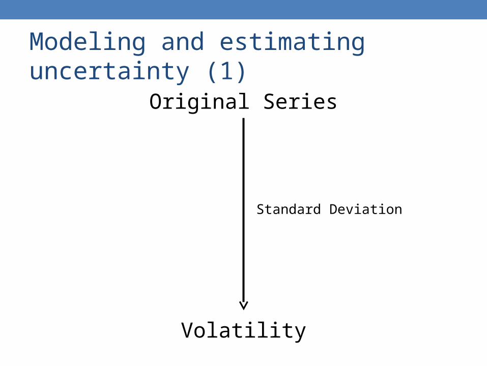
Modeling and estimating uncertainty (1)

Original Series

Volatility

Standard Deviation

Modeling and estimating uncertainty (2)

Original Series

Detrended Residuals

Volatility

HP Filter / Polynomial Detrending

Standard Deviation

Modeling and estimating uncertainty (3)

Original Series

Detrended Residuals

Detrended + Decycled Residuals

Volatility

HP Filter / Polynomial Detrending

Fourier Decomposition

Standard Deviation

Empirical proxies for volatility in the literature

SD of raw series

• Aizenman et al. (2011), “Adjustment patterns to commodity terms of trade shocks: the role of exchange rate and international reserves policies”, NBER WP 17692.

• Larrain & Parro (2006), “Chile menos volátil”, Instituto de Economía, Universidad Católica de Chile.

• Mendoza (1994), “Terms-of-trade uncertainty and economic growth. Are risk indicators significant in growth regressions?”, International Finance Discussion Papers (Vol 491).

SD of detrended residuals

Distinguish between predictable (regular part) and unpredictable (uncertainty) components of a variable.

• Kim (2007), “Openness, external risk, and volatility: implications for the compensation hypothesis”, Cambridge Univ Press.

• Wolf (2004), “Volatility: Definitions and Consequences”, Draft Chapter for Managing Volatility and Crises.

• Dehn (2000), "Commodity price uncertainty in developing countries”, World Bank (Series 2426)

• Baxter (2000), “International trade and business cycles”, in Grossman and Rogoff .

Empirical proxies for volatility in the literature

How to determine the residuals: warnings about proper detrending

“Much care has to be dedicated to the detrending procedure since a wrong specification can bias severely the subsequent analysis” (Bee Dagum)

“Different detrending procedures are alternative windows which look at the series from different perspectives” (Canova)

• Bee Dagum et al. (2006), “A critical investigation on detrending procedures for non-linear processes”, Journal of Macroeconomics (vol 28).

• Kauermann et al. (2008), “Smoothing parameter selection for spline estimation”,

• Kauermann et al. (2011), "Filtering time series with penalized splines", Studies in Nonlinear Dynamics and Econometrics, (vol 15(2))

• Canova (1998), “Detrending and business cycle facts: A user’s guide”, Journal of Monetary Economics (vol 41).

Data and procedureData:Argentina TOT and GDP logged from index1993=100. 1810 – 2010 (Ferreres & INDEC)

Detrending:a. Cubic polynomial detrendingb. HP filter detrending (lambda = 100)

Decycling:a. Fourier decomposition

TOT and GDP cubic polynomial detrending

-.6

-.4

-.2

.0

.2

.4

.6

3.2

3.6

4.0

4.4

4.8

5.2

1825 1850 1875 1900 1925 1950 1975 2000

Residual Actual Fitted

-.4

-.2

.0

.2

.4

.6

6

8

10

12

14

1825 1850 1875 1900 1925 1950 1975 2000

Residual Actual Fitted

TOT Cubic DetrendingTrend and Residuals

GDP Cubic DetrendingTrend and Residuals

Fourier decompositionFollowing Bolch and Huang, the decomposition of a series into its periodic components is done using:

where

and

101 101

0 0

cos 2 sin 2at i ii i

t tZ i iT T

ˆat at atZ Y Y

1 logt tY TOT 2 logt tY GDP

Fourier decomposition

Relative Cumulative

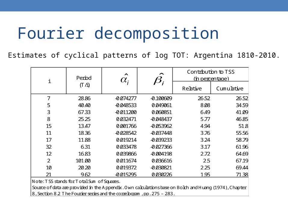
7 28.86 -0.074277 -0.100609 26.52 26.525 40.40 -0.048533 0.049061 8.08 34.593 67.33 -0.011200 0.060851 6.49 41.098 25.25 0.032471 -0.048437 5.77 46.8515 13.47 0.001766 -0.053962 4.94 51.811 18.36 -0.028542 -0.037448 3.76 55.5617 11.88 0.019214 -0.039233 3.24 58.7932 6.31 0.033478 -0.027366 3.17 61.9612 16.83 0.039866 -0.004198 2.72 64.692 101.00 0.011674 0.036616 2.5 67.1910 20.20 0.019372 -0.030821 2.25 69.4421 9.62 -0.015295 0.030226 1.95 71.38

Contribution to TSS(in percentage)

Note: TSS stands for Total Sum of Squares. Source of data are provided in the Appendix. Own calculations base on Bolch and Huang (1974), Chapter 8, Section 8.2 The Fourier series and the correlogram, pp. 275 – 283.

iPeriod(T/i)

Estimates of cyclical patterns of log TOT: Argentina 1810-2010.

ˆi

i

Comments on TOT decomposition I. The most important cycle:• period: 28.86 years • frequency: observed only seven times in 202

years • acounts for 26.52% of the total sum of squares.

II. The first five most important cycles account for 51.8% of the total sum of squares

Relative Cumulative

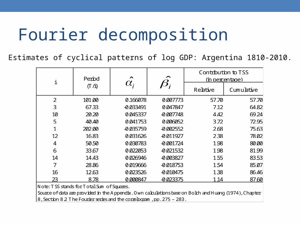
2 101.00 0.166078 0.007773 57.70 57.703 67.33 -0.033491 0.047847 7.12 64.8210 20.20 0.045337 -0.007748 4.42 69.245 40.40 0.041753 0.006052 3.72 72.951 202.00 -0.035759 -0.002552 2.68 75.6312 16.83 0.031626 -0.011927 2.38 78.024 50.50 0.030783 -0.001724 1.98 80.006 33.67 0.022053 -0.021532 1.98 81.9914 14.43 0.026946 -0.003827 1.55 83.537 28.86 0.019666 -0.018753 1.54 85.0716 12.63 0.023526 -0.010475 1.38 86.4623 8.78 0.000847 -0.023375 1.14 87.60

Contribution to TSS(in percentage)

Note: TSS stands for Total Sum of Squares. Source of data are provided in the Appendix. Own calculations base on Bolch and Huang (1974), Chapter 8, Section 8.2 The Fourier series and the correlogram, pp. 275 – 283.

iPeriod(T/i)

Fourier decompositionEstimates of cyclical patterns of log GDP: Argentina 1810-2010.

ˆi

i

Comments on GDP decomposition (1)I. The most important cycle:• period: 101 years • frequency: observed twice in 202 years • acounts for 57.70 percent of the total sum of

squares.

II. Another important cycle:• Period: 202 years • frequency: observed once in 202 years • acounts for 2.68 percent of the total sum of

squares.

Is it meaningful to assume that the 202-year super-cycle exists as a long run

process of GDP?

•Cycles should not be taken mechanically

•Their economic relevance has not a clear interpretation

For analytical purposes we have kept all cycles

Comments on GDP decomposition (2)

How many of the cycles are to be removed from the detrended series?

• For TOT we extracted approximately 55% of variability

• For GDP we extracted approximately 80% of variability

The results obtained proved to be robust to different choices of end points

Removed cycles and decycled residuals

-.3

-.2

-.1

.0

.1

.2

.3

.4

1825 1850 1875 1900 1925 1950 1975 2000

TOT Removed Cycles

-.3

-.2

-.1

.0

.1

.2

.3

.4

1825 1850 1875 1900 1925 1950 1975 2000

GDP Removed Cycles

-.3

-.2

-.1

.0

.1

.2

.3

.4

1825 1850 1875 1900 1925 1950 1975 2000

Decycling TOT

-.3

-.2

-.1

.0

.1

.2

.3

1825 1850 1875 1900 1925 1950 1975 2000

Decycling GDPDecycled TOT Decycled GDP

TOT Removed Cycles GDP Removed Cycles

This measure drops monotonically when more knowledge on cycles is attributed to the

economic agents

TOT GDP

SD SD

0 0.172 0.152

1 0.146 0.099

2 0.137 0.089

3 0.130 0.084

4 0.124 0.079

5 0.118 0.074

6 0.112 0.071

7 0.108 0.068

8 0.104 0.065

9 0.101 0.062

10 0.097 0.059

Number of cycles removed

Note: SD stands for standard deviation.Source of data: Own estimations

A scalar measure of volatility (1810-2010)

Volatility = SD in a five-year rolling sample

of the decycled residual series

A proxy for volatility

TOT and GDP volatility (1815-2010) SD (five years) of cubic detrending and Fourier decycling

.00

.05

.10

.15

.20

.25

1850 1900 1950 2000

TOT Volatility

.00

.05

.10

.15

.20

.25

1850 1900 1950 2000

GDP VolatilityTOT volatility

(extracting 55% of variability)GDP volatility

(extracting 80% of variability)

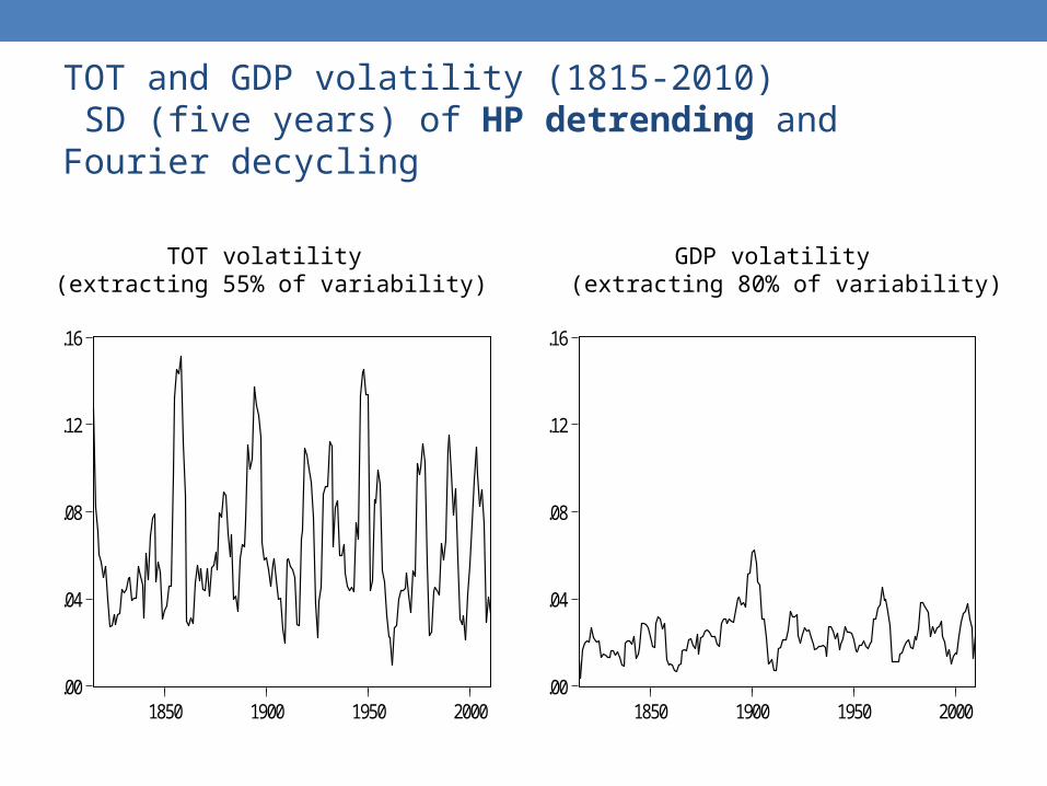
TOT and GDP volatility (1815-2010) SD (five years) of HP detrending and Fourier decycling

TOT volatility (extracting 55% of variability)

GDP volatility (extracting 80% of variability)

.00

.04

.08

.12

.16

1850 1900 1950 2000

SD of log tot detrending (HP) and decycling(extrancting 55% of variability)

.00

.04

.08

.12

.16

1850 1900 1950 2000

SD of log GDP detrending (HP) and decycling(extrancting 80% of variability)

IIIAnalysis of the results

Is TOT volatility overestimated in empirical analysis?

SD of TOT HP residuals

SD of TOT detrendig (HP) and decycled

Mean  0.087  0.064Std. Dev.  0.044  0.031

.00

.04

.08

.12

.16

.20

.24

1825 1850 1875 1900 1925 1950 1975 2000

SD of TOT HP residualsSD of TOT detrendig and decycling

Is GDP volatility overestimated in empirical analysis?

.00

.02

.04

.06

.08

.10

.12

1825 1850 1875 1900 1925 1950 1975 2000

SD of GDP detrendig and decyclingSD of GDP HP residuals

SD of GDP HP

residuals

SD of GDP detrendig (HP) and

decycled

 Mean  0.039  0.023 Std. Dev.  0.027  0.010

Does TOT volatility Granger-cause GDP volatility?

Is it the level, trend, cycles, volatility or other statistical property of TOT relevant?

Do TOT affect the level, the volatility, the growth rate or some other characteristic of GDP?

If there is a relation between them, which is its sign?

Insights of TOT volatility effects

Evidence related to causality is very heterogeneous

Many variables (degree of openness, concentration of X and M, the financial system, etc.) may explain the heterogeneous empirical

results

Direct relationship between TOT volatility and GDP volatility seems to prevail in the

literature

TOT index positive trend, and large fluctuations.Irregular GDP growth

20

40

60

80

100

120

140

160

1825 1850 1875 1900 1925 1950 1975 2000

TOT

-.3

-.2

-.1

.0

.1

.2

.3

1825 1850 1875 1900 1925 1950 1975 2000

GDPTOT index 1993=100 (1810-2010)

GDP growth (1811-2010)

1909: 146

1987: 852000: 1062010: 141

1948: 150

1922: 71

1897: -21%2001: - 13%

1890: -8% Baring Crisis

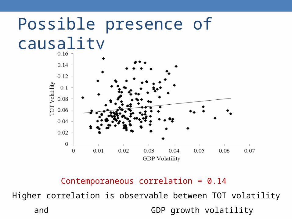
Possible presence of causality

Contemporaneous correlation = 0.14

Higher correlation is observable between TOT volatility and

GDP growth volatility

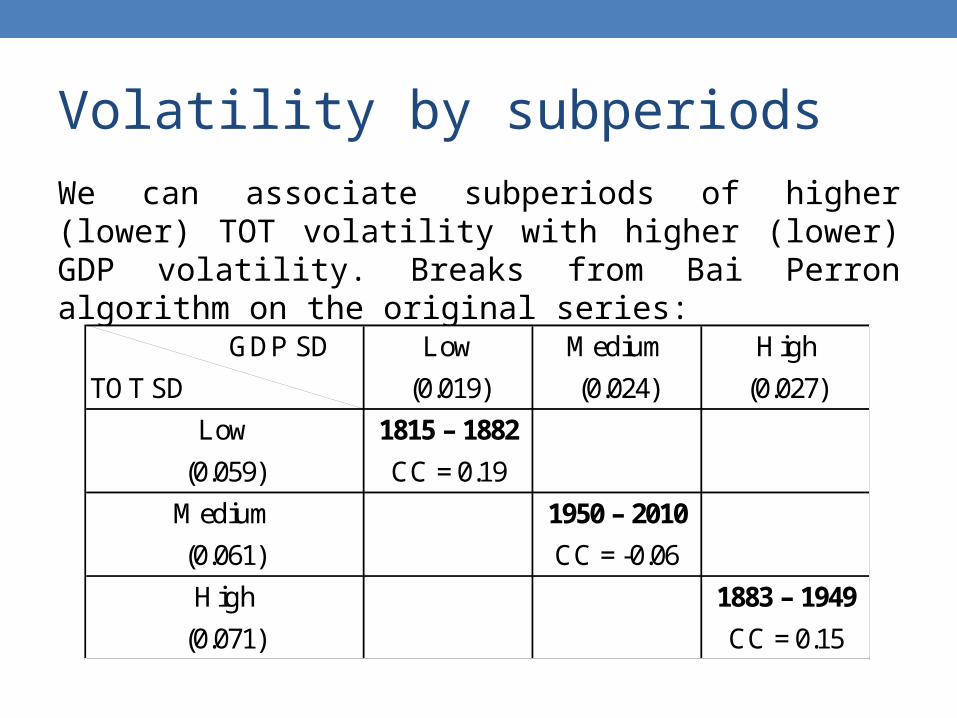
Volatility by subperiodsWe can associate subperiods of higher (lower) TOT volatility with higher (lower) GDP volatility. Breaks from Bai Perron algorithm on the original series:

GDP SD

TOT SD

1815 – 1882

CC = 0.19

1950 – 2010

CC = -0.06

1883 – 1949

CC = 0.15

Low

(0.019)

Medium

(0.024)

High

(0.027)

Low

(0.059)

Medium

(0.061)

High

(0.071)

Exercise on VAR estimationSpecifications:

• Assumption of small open economy – SOE

• Variables (in order):

SD (five years) of TOT detrending and decycled residuals

SD (five years) of GDP detrending and decycled residuals

• Sample: 1815 – 2010

• Control variables: grade of openness, export price index, investment.

VAR impulse response functionOnce-and-for-all 1-standard deviation shock

to TOT volatility on GDP volatility

IVConcluding remarks

Concluding remarks• Alternative definitions of volatility may be used to measure the degree of uncertainty in the evolution of an economic variable.

• From a methodological point of view the variability of an economic time series overestimates its volatility.

• The choice of a specific method might impinge on the magnitude, and other statistical properties of the volatility of a variable.

• Relevant structural features of the Argentine economy determined by its land abundance: concentration of exports on agricultural commodities generates volatility on TOT.

• Impact on income distribution, external liquidity and solvency, instability of fiscal budgets, preference for flexibility on investment.

Policy implications

Extensions• Identification of statistical breaks in TOT volatility. Cubic Splines Detrending.

• Further modeling with regard to the relationship between TOT volatility and GDP volatility. Channels of transmition. Control variables (Investment, Grade of Openness, Balance of Payments, etc). Not readily available over such long time span.

• We use barte TOT. Berlinski (2003) documented a wide gap between internal and external terms of trade.

Extensions Continued• Sudden TOT changes bring about severe distributive conflicts because Argentina is a big exporter of wage goods.

• Wolf (2004): uncertainty proxied by SD might be better measured by a weighting procedure which does not rely on symmetry.

• Wolf (2004): the relationship between TOT and GDP may be subject to threshold effects not captured by a linear model.

Thank You

Assessing terms of trade volatility in Argentina

1810 - 2010.A Fourier approach to decycling.

José Luis ArrufatAlberto M. Díaz Cafferata

María Victoria AnauatiSantiago Gastelu

Instituto de Economía y Finanzas. Facultad de Ciencias Económicas

Universidad Nacional de Córdoba

ReferencesAizenmanEdwardsRiera-Crichton (2011)Larrain, Parro (2006)Mendoza (1994)Kim (2007)Wolf (2004)Dehn (2000)Baxter (2000)