Al

JJa

b

c

d

e

a

ARRA

KCDSVW

1

trti2vgrcvteaaie

0h

Ecological Modelling 266 (2013) 131– 143

Contents lists available at ScienceDirect

Ecological Modelling

jo ur nal ho me page: www.elsev ier .com/ locate /eco lmodel

ssessing potential climate change effects on vegetation using ainked model approach

essica E. Halofskya,∗, Miles A. Hemstromb, David R. Conklinc,oshua S. Halofskyd, Becky K. Kernse, Dominique Bacheletc

School of Environmental and Forest Sciences, University of Washington, Box 352100, Seattle, WA 98195-2100, USAUSDA Forest Service, Forestry Sciences Laboratory, 620 SW Main St., Suite 400, Portland, OR 97205, USAConservation Biology Institute, 136 SW Washington Avenue, Suite 202, Corvallis, OR 97333, USAWashington Department of Natural Resources, PO Box 47000, 1111 Washington Street SE, Olympia, WA 98504-7000, USAUSDA Forest Service, Forestry Sciences Laboratory, 3200 SW Jefferson Way, Corvallis, OR 97331, USA

r t i c l e i n f o

rticle history:eceived 21 February 2013eceived in revised form 14 June 2013ccepted 1 July 2013

eywords:limate change

a b s t r a c t

We developed a process that links the mechanistic power of dynamic global vegetation models withthe detailed vegetation dynamics of state-and-transition models to project local vegetation shifts drivenby projected climate change. We applied our approach to central Oregon (USA) ecosystems using threeclimate change scenarios to assess potential future changes in species composition and community struc-ture. Our results suggest that: (1) legacy effects incorporated in state-and-transition models realisticallydampen climate change effects on vegetation; (2) species-specific response to fire built into state-and-

ynamic global vegetation modelstate-and-transition modelsegetation dynamicsildfire

transition models can result in increased resistance to climate change, as was the case for ponderosa pine(Pinus ponderosa) forests, or increased sensitivity to climate change, as was the case for some shrublandsand grasslands in the study area; and (3) vegetation could remain relatively stable in the short term,then shift rapidly as a consequence of increased disturbance such as wildfire and altered environmentalconditions. Managers and other land stewards can use results from our linked models to better anticipatepotential climate-induced shifts in local vegetation and resulting effects on wildlife habitat.

. Introduction

Climate, in concert with local topoedaphic factors, dictates vege-ation distribution through thermal and water constraints on plantegeneration, establishment, growth, and mortality. Global vegeta-ion patterns are already shifting in response to observed increasesn temperature and changing precipitation patterns (Parmesan,006; Allen et al., 2010). Anticipating potential shifts in localegetation is critical for land managers to develop adaptive strate-ies. However, predicting vegetation response to climate changeequires consideration of interacting physical and biological pro-esses at multiple spatial and temporal scales. Dynamic globalegetation models (DGVMs) are currently considered to be amonghe most advanced tools to assess climate change effects oncosystems (Fischlin et al., 2007). DGVMs integrate state-of-the-rt knowledge of plant physiology, biogeography, biogeochemistry,

nd biophysics, with climate model projections to simulate changesn vegetation structure and composition (biogeography) as well ascosystem function (biogeochemistry) through time (Prentice et al.,

∗ Corresponding author. Tel.: +1 206 543 9138.E-mail address: jhalo@uw.edu (J.E. Halofsky).

304-3800/$ – see front matter © 2013 Elsevier B.V. All rights reserved.ttp://dx.doi.org/10.1016/j.ecolmodel.2013.07.003

© 2013 Elsevier B.V. All rights reserved.

1989, 2007; Foley et al., 1998; Cramer et al., 2001). MC1 (Daly et al.,2000; Bachelet et al., 2001) is a DGVM that integrates biogeogra-phy, biogeochemistry, and fire into a single modeling environmentand has been used for regional- to global-scale assessments ofpotential climate change effects on ecosystems (e.g., Bachelet et al.,2000, 2003; Lenihan et al., 2008a,b; Gonzalez et al., 2010; Rogerset al., 2011; Shaw et al., 2011). DGVMs simulate broad plant func-tional types that combine numerous species into single entities(e.g., evergreen needleleaf trees), and thus they are incapable ofsimulating community- and species-level changes at the landscapescale (Hickler et al., 2004). However, because they focus on mecha-nisms, their projections of future outcomes are more reliable thansimple correlations of location with current climate conditions. Totake full advantage of their strength, their results can be translatedinto directions and magnitude of change applicable to community-and species-level dynamics, making output more useful for sub-regional management and planning efforts (e.g., Halofsky et al.,2011).

State-and-transition models (STMs) simulate trends in veg-

etation community response to a variety of local disturbancesand management strategies by explicitly incorporating landscapelegacy, succession rules and species-specific sensitivity to disturb-ance. STMs are based on transition matrix methods that simulate

1 l Mod

vtersbFtcrF2lpsaetAc

lsvScaitiO

2

2

ag2dtc

32 J.E. Halofsky et al. / Ecologica

egetation dynamics using transition probabilities between vege-ation states (e.g., Horn, 1975; Noble and Slatyer, 1980; Westobyt al., 1989; Laycock, 1991). The landscape is divided into statesepresenting combinations of cover type (dominant species) andtructural stage (e.g., diameter class, canopy density, and num-er of canopy layers) within a particular biophysical environment.or example, a state could represent dry ponderosa pine forest inhe 25–38 cm diameter class with closed tree canopy and a singleanopy layer. States are linked by transitions that represent natu-al disturbances, management actions, or successional processes.or example, high-severity fire could drive a ponderosa pine forest,5–38 cm diameter class, closed-canopy state to an open grass-

and state. STMs are run at scales appropriate for management andlanning efforts (units typically range from 10 s to 1000 s of ha inize). They have been extensively used for regional to sub-regionalssessments (e.g., Hemstrom et al., 2001, 2002, 2007; Merzenicht al., 2003; Forbis et al., 2006; Weisz et al., 2009). However, withhe exception of some very recent developments (Provencher andnderson, 2011), STMs have not incorporated the effects of climatehange.

Here we present results from a novel modeling approach thatinks the mechanistic power of a DGVM with the community-pecific control of state-and-transition models to project localegetation shifts. We linked a DGVM (MC1) with a set of eightTMs, each representing a major vegetation type in a study area inentral Oregon, to assess potential changes in species compositionnd community structure under different climate change scenar-os. Our objectives are to (1) describe the approach we used to linkhe DGVM with STMs; and (2) project potential future changesn species composition and community structure for the centralregon study area.

. Materials and methods

.1. Study area

The study area is a landscape of forests, woodlands, shrublands,nd grasslands that is 1,023,808 ha in size, located in central Ore-on, USA (Fig. 1). Elevations vary from about 1200 m to above

400 m. The climate is transitional between moist, maritime con-itions west of the Cascade Mountains (which are oriented northo south; Fig. 1) and continental conditions to the east. Annual pre-ipitation varies from over 2000 mm along the Cascade Crest to less

Fig. 1. Study area in central Oregon, USA. Ecoregions show

elling 266 (2013) 131– 143

than 350 mm along lower treeline and 250 mm at the lowest eleva-tions in shrub-steppe environments (PRISM Group, 2012). Most ofthe precipitation falls as rain and snow during the winter months,with snow packs of more than 2 m common in upper elevations.Summers are warm and dry, often with several weeks of very lowor no precipitation and warmest temperatures at lower elevationsexceeding 30 ◦C.

2.2. The MC1 model

MC1 (Bachelet et al., 2001) is a DGVM that simulates: life-form mixtures, classifying them into potential vegetation classes(PVCs); the fluxes and pools of carbon, nitrogen, and water throughecosystems; and natural fire occurrence and effects. MC1 rou-tinely generates century-long, local to global-scale simulations(e.g., Bachelet et al., 2003; Daly et al., 2000; Lenihan et al., 2003,2008a; Hayhoe et al., 2005; Rogers et al., 2011). The model readssoil and monthly climate data, and calls interacting modules thatsimulate biogeography, biogeochemistry, and fire disturbance.

The biogeography module, which was developed using some ofthe biogeography rules from the MAPSS model (Neilson, 1995), sim-ulates life-form mixtures of evergreen needleleaf or broadleaf, anddeciduous needleleaf or broadleaf trees, as well as temperate (C3)and warm-season (C4) grasses. An algorithm is used to determinelife-form mixture at each annual time-step as a function of annualaverage minimum monthly temperature and growing season pre-cipitation (see Bachelet et al., 2001; Daly et al., 2000). Tree andgrass life-form mixtures, their biomass simulated by the biogeo-chemistry module, as well as climate indices are used to determinewhich of several dozen possible PVCs occurs in each simulated gridcell each year (see Bachelet et al., 2001; Daly et al., 2000).

The biogeochemistry module is a modified version of the CEN-TURY model (Parton et al., 1993), which simulates plant growth,organic matter decomposition, and the movement of water andnutrients through ecosystems. The biomass and hydrology algo-rithms from CENTURY were retained and linked to the dynamicbiogeography driver. Life-form specific parameters (e.g., maximumproduction rate of evergreen trees) are determined annually bymodifying their original values as a function of their dominance

along the two-dimensional climatic gradient defined by growingseason precipitation and annual average minimum monthly tem-perature (Bachelet et al., 2001). In this study, plant growth wasassumed not to be limited by nutrient availability; the nitrogen

n are Omernik Level III Ecoregions (Omernik, 1987).

l Mod

dtottmpbalw

rfipfCaotb([mcie

deaesferoTatmfafeo

2

stsudgdfiCmCuctb

J.E. Halofsky et al. / Ecologica

emand was estimated and met assuming biological nitrogen fixa-ion would provide what deposition did not. The direct effect of thebserved increase in atmospheric carbon dioxide (CO2) concentra-ion was simulated using a beta factor (Friedlingstein et al., 1995)hat increases maximum potential productivity and reduces the

oisture constraint on productivity. Grasses compete with woodylants for soil moisture and nutrients in the upper soil layers whereoth are rooted, while the deeper-rooted woody plants have soleccess to water in deeper layers. The growth of grasses is alsoimited by reduced light levels due to increased plant density as

ell as shading by woody plants.The MC1 fire module (Lenihan et al., 1998) simulates the occur-

ence, behavior, and effects of fire in all PVCs. The model simulatesre initiation and the behavior of a fire event in terms of theotential rate of fire spread, fireline intensity, and the transitionrom surface to crown fire (Rothermel, 1972; van Wagner, 1973;ohen and Deeming, 1985). Estimates of fuel bed characteristicsre required to simulate fire behavior, and are provided by thether two MC1 modules. The current life-form mixture is usedo select factors that allocate the simulated live and dead car-on pools into classes of live fuels (grass leaves) and dead fuels1-h [<0.64 cm diameter], 10-h [0.64–2.54 cm diameter], 100-h2.54–7.6 cm diameter], and 1000-h [7.6–20.3 cm diameter]). The

oisture content of the live fuels is derived from soil moisture cal-ulated in the biogeochemistry module. Dead fuel moisture contents estimated from the climate drivers using different functions forach of four dead fuel size-classes (Cohen and Deeming, 1985).

Fire events are initiated in the model when the fine fuel moisturerops below a defined threshold and fuel buildup simultaneouslyxceeds a defined threshold. Sources of ignition (e.g., lightning)re assumed to be always available. Area burned is not simulatedxplicitly as fire spread within a given cell (potential rate of firepread, mentioned above, is used to determine plant mortality anduel consumption); instead, the fraction of a cell burned by a firevent is estimated as a function of set minimum and maximum fireeturn intervals for the dynamically-simulated PVC and the numberf years since the last simulated fire event (Lenihan et al., 2008a).he fire effects simulated by the model include plant mortalitynd consumption of vegetation carbon, which is removed from (orransferred to) the appropriate carbon pools in the biogeochemistry

odule. Fire-driven mortality and consumption are simulated as aunction of fireline intensity and tree canopy structure (Petersonnd Ryan, 1986). Dead biomass consumption is simulated usingunctions of fuel moisture that are fuel-class specific (Andersont al., 2005). See Bachelet et al. (2001) for additional informationn general MC1 model formulation and parameterization.

.3. Climate projections

Climate data sets required for running the MC1 model in thistudy consisted of monthly values of four variables: precipitation,he monthly means of diurnal extreme temperatures, and a mea-ure of atmospheric water content. For the historical period, wesed the PRISM (Parameter–elevation Relationships on Indepen-ent Slopes Model) climate data set on a 30-arcsec grid (∼800 mrain; Daly et al., 1997, 2008). The PRISM group provided monthlyata for the years 1895–2008 for the conterminous U.S. Threeuture climate projections from general circulation models (GCMs)ncluded in the World Climate Research Programme’s (WCRP’s)oupled Model Intercomparison Project phase 3 (CMIP3) multi-odel dataset and subsequently in the Intergovernmental Panel on

limate Change (IPCC) Fourth Assessment Report (IPCC, 2007) were

sed to drive MC1 projections for the 21st century. We obtainedomplete time series of the four necessary climate variables fromhe data repository at Lawrence Livermore Laboratories producedy the MIROC 3.2 medres (Hasumi and Emori, 2004), CSIRO Mk3

elling 266 (2013) 131– 143 133

(Gordon et al., 2002), and Hadley CM3 (Gordon et al., 2000; Johnset al., 2003) GCMs (hereafter MIROC, CSIRO, and Hadley, respec-tively) for the IPCC SRES A2 emissions scenario (Nakicenovic andSwart, 2000). We used the A2 carbon dioxide emissions scenario. Afull century transient series from 2010 to 2100 was used as inputto MC1.

Mote and Salathé (2010) compared projections from 21 GCMsused in the IPCC AR4 to historical climate data (University of EastAnglia Climatic Research Unit version 2.02; Mitchell et al., 2004)for the Pacific Northwest over the 1970–1999 period. Comparedto the other models assessed by Mote and Salathé (2010), Hadleyproduced a relatively low precipitation bias (or mean differencebetween model projections and historical climate data; both annu-ally and seasonally), but failed to show an increasing trend in meanannual temperature over the 20th century. MIROC showed a rela-tively low temperature bias but high precipitation bias. CSIRO wasranked highest for reproducing the trend in mean annual temper-ature over the 20th century, but had a high positive temperaturebias.

For the U.S. Pacific Northwest, CSIRO projects a relatively cooland wet future conditions (+2.6 ◦C and +176 mm mean annualprecipitation in 2070–2099), MIROC projects relatively hot andwet conditions (+4.2 ◦C and +82 mm mean annual precipitation in2070–2099), and Hadley projects relatively hot and dry conditions(+4.2 ◦C and −78 mm mean annual precipitation in 2070–2099)(Rogers et al., 2011). For all three GCMs, temperature increasesare generally greater in summer than in winter, while precipita-tion increases in winter and decreases in summer. Mean monthlysummer (June, July, August) precipitation decreases by as much as5 mm under CSIRO, 10 mm under MIROC, and 15 mm under Hadley,with historical mean monthly summer precipitation of 30–50 mmover most of Oregon and Washington (Rogers et al., 2011).

The spatial grids used by the MIROC, CSIRO, and Hadley GCMsare coarse (2.8 × 2.8 degrees for MIROC, 1.9 × 1.9 degrees for CSIRO,and 2.5 × 3.75 degrees for Hadley). We down-scaled the coarsegrid GCM data to a 30-arcsec grid using a “delta” or “anomaly”method (Fowler et al., 2007). We first calculated a historical climatebaseline (mean values for each month) for 1971–2000, our refer-ence period, using PRISM data. We also calculated a coarse-scalehistorical baseline for the same reference period using the GCMprojections. Secondly, for each month of each year of the futureperiod, we calculated the difference (for temperature and vaporpressure) or the ratio (for precipitation) of the future value and thereference historical baseline climate from each GCM (the “delta”).We then down-scaled the coarse-scale deltas to the fine (30-arcsec)grid using bilinear interpolation. Finally, we calculated the fine gridclimate values for each month of each year of the future periodusing the PRISM historical baseline modified by the fine-scale deltas(meaning that topographic effects are incorporated in the down-scaled climate data to the extent that they are represented in thePRISIM data). Difference deltas were added to the baseline whileratio deltas were multiplied with the baseline.

2.4. State-and-transition models (STMs)

The STM approach characterizes vegetation in terms of statesthat are linked together by transitions, which describe processesthat cause change among vegetation states (Westoby et al., 1989;Laycock, 1991). We used, and in some cases modified, previously-developed STMs for our study area (Hann et al., 1997; The NatureConservancy, 2006; Hemstrom et al., 2007; Evers, 2010). ExistingSTMs were developed in the Vegetation Development Dynamics

Tool (VDDT; ESSA Technologies Ltd., 2007). VDDT is stand-alonesoftware that allows development of STMs and simulates vege-tation dynamics by dividing the landscape into states, assigningprobabilities to transitions between states, and simulating the state

134 J.E. Halofsky et al. / Ecological Modelling 266 (2013) 131– 143

Fig. 2. (a) Potential vegetation types mapped from imputation of inventory plots, and (b) potential vegetation classes simulated by MC1 for the recent historical period( getatic atially

obmob((iSp

itcrslo(Paifg

d

1971–2000). We matched the potential vegetation types in (a) to corresponding velass corresponded with multiple potential vegetation types, we chose the most sp

f the landscape over time using Monte Carlo methods. Transitionsetween states may be either deterministic or probabilistic. Deter-inistic transitions are specified to occur after a certain number

f time steps within a state (e.g., succession), whereas proba-ilistic transitions are defined by an annual transition probabilitye.g., wildfire). Recently, VDDT was folded into the Path interfaceApexRMS and ESSA, 2011), which has improved model build-ng and analysis features and facilitates running spatially-explicitTMs. Thus, model simulations were run using the Path modelinglatform using annual time-steps.

The previously-developed set of STMs used for this studyncluded 11 STMs, each representing a single potential vegeta-ion type (PVT; Fig. 2a). However, to incorporate climate-inducedhanges in vegetation from MC1 in the STMs, we chose a rep-esentative STM for each PVC that was simulated by MC1 in thetudy area. To choose representative STMs, we used spatial over-ays of historical (1971–2000) MC1 results (Fig. 2b) and our mapsf current PVT distribution (Fig. 2a), generating a crosswalk tableTable 1). In cases where a single PVC corresponded with multipleVTs, we chose the most spatially extensive PVT within the PVCrea. MC1 simulations for the future showed a new PVC occurringn the study area, warm-season grassland. Thus, we chose an STM

rom a more southern modeling zone to represent warm-seasonrassland.

Previously-developed STMs for the study area were indepen-ent, meaning that once a given area of land was classified into a

on classes in (b) using spatial overlays. In cases where a single potential vegetation extensive potential vegetation type within the potential vegetation class area.

certain PVT, represented by a single STM, it could not be reclassifiedinto another PVT over time in the model simulations. Thus, whilea given area could move among different states within an indi-vidual STM over time due to management, natural disturbances,and vegetation development, that area could not change PVTs. Wechanged this by modifying the model structure, developing onelarge interconnected STM, and allowing shifts among PVTs with cli-mate change and disturbance. We assumed that the PVC changesprojected by MC1 could be approximated by changes among similaror representative PVTs that currently exist in the study area or occurin adjacent landscapes (Table 1). Our selected PVTs are used to rep-resent future vegetation types that we assume will have generallysimilar internal vegetation dynamics and disturbance relations.

STMs for forested PVTs (large green boxes in Fig. 3) includedstates (combinations of vegetation composition and structure;small gray boxes in Fig. 3) defined by overstory cover type andstructural conditions. Cover types were defined by the dominanttree species in the upper-most canopy layer. For example, theSTM for the ponderosa pine-lodgepole pine PVT included bothponderosa pine and lodgepole pine cover types. Within covertypes, structural classes were defined by combinations of treediameter class (quadratic mean diameter of the largest 20% of

the trees; 0 cm Diameter at Breast Height (DBH) = Grass/forb;<13 cm DBH = seedling/sapling; 13–25 cm DBH = pole; 25–38 cmDBH = small; 38–51 cm DBH = medium; 51–76 cm DBH = large;>76 cm DBH = giant), overstory canopy cover (<10% = grass/forb,

J.E. Halofsky et al. / Ecological Modelling 266 (2013) 131– 143 135

Table 1MC1 potential vegetation classes and their corresponding state-and-transition model (STM) potential vegetation types in the study area. We chose one representative STMfor each MC1 potential vegetation class (representative STMs are underlined in the STM potential vegetation type column). Mapped current extent is derived from imputationof inventory plot characteristics across the study area. MC1 current extent represents current conditions as simulated by the MC1 model.

MC1 potential vegetation classes STM potential vegetation types Common species Imputed currentextent (%)

MC1 currentextent (%)

Subalpine forest Mountain hemlock andsubalpine fir forests

Mountain hemlock (Tsuga mertensiana), whitebarkpine (Pinus albicaulis), Engelmann spruce (Piceaengelmannii), subalpine fir (Abies lasiocarpa), andlodgepole pine (Pinus contorta)

2 2

Cool needleleaf forest Moist mixed conifer forests Douglas-fir (Pseudotsuga menziesii), white fir (Abiesconcolor), Shasta red fir (Abies × shastensis[magnifica × procera]), ponderosa pine (Pinusponderosa), western hemlock (Tsuga heterophylla),and western redcedar (Thuja plicata)

11 4

Temperate needleleaf forest Ponderosa pine, lodgepolepine, and dry mixed coniferforests

Ponderosa pine, lodgepole pine, Douglas-fir, andgrand fir (Abies grandis)

59 67

Temperate needleleaf woodland Mountain big sage—westernjuniper woodland andshrubland

Western juniper (Juniperus occidentalis), andmountain big sagebrush (Artemisia tridentata ssp.vaseyana)

14 6

Temperate shrubland Wyoming big sage shrubland Wyoming big sagebrush (Artemisia tridentata ssp.wyomingensis), and antelope bitterbrush (Purshiatridentata)

12 18

Xeromorphic shrubland Salt desert shrubland Greasewood (Sarcobatus vermiculatus), saltbush(Atriplex canescens), and Wyoming big sagebrush

2 <1

Temperate grassland Bluebunchwheatgrass–Sandberg

Idaho fescue (Festuca idahoensis), bluebunchwheatgrass (Pseudoroegneria spicata), and

rass (B

<1 3

(Pleu

1lecrwsfi(teibeWl

s

Fsabrr

bluegrass grassland cheatgWarm-season grassland Warm-season grassland Galleta

0–40% = low, 40–60% = medium, >60% = high), and canopyayering (single or multiple). A grass-forb state representedarly-successional conditions before establishment of a signifi-ant tree canopy. We also included post-disturbance states thatesulted from a stand-replacing disturbance (insect outbreak orildfire) prior to any salvage logging and, consequently, containing

tanding snags and downed wood. In similar fashion, our STMsor arid land PVTs (all woodlands, shrublands, and grasslandsn Table 1) included vegetation states defined by cover typesdominant species composition) and structural conditions. Coverypes reflected varying amounts of native, semi-degraded, andxotic herbaceous and shrub states, and different phases of junipernvasion, where applicable. For example, the STM for the Wyomingig sage shrubland PVT included both Wyoming big sage withxotic annual grasses and native perennial grass cover types.ithin cover types, structural classes reflected percent cover by

ife-form (grasses, shrubs, or trees).To characterize the PVT (Fig. 3a) for each 30-m pixel on the land-

cape and determine which STM to use for that pixel, we acquired

ig. 3. Simplified illustration of state-and-transition models (STMs; green boxes), each rtates (combinations of vegetation composition and structure; gray boxes), with transitind succession. To incorporate climate change in our set of previously-independent STMsased on MC1 vegetation change and fire output (red arrows). Transitions among PVTs oepresented by State A). Our actual climate-informed STM included eight potential vegeferences to color in this figure legend, the reader is referred to the web version of this a

romus tectorum) (non-native)raphis spp.) 0 0

forested PVT maps from ecoshare (http://ecoshare.info/), and aridlands PVT maps were downloaded from the Integrated LandscapeAssessment Project website (http://oregonstate.edu/inr/ilap/). Toinform initial vegetation conditions (vegetation composition andstructure, i.e., states) for each 30-m pixel within a PVT, existingvegetation maps for forests were downloaded from the Land-scape Ecology, Modeling, Mapping and Analysis website (LEMMA,http://www.fsl.orst.edu/lemma), and existing vegetation maps forarid lands were downloaded from the Integrated Landscape Assess-ment Project website (http://oregonstate.edu/inr/ilap/). Both PVTand existing vegetation maps were derived from imputations of themeasured vegetation in inventory plots to 30-m pixels using gra-dient nearest neighbor (Ohmann and Gregory, 2002) and randomforest methods (Crookston and Finley, 2007). These methods essen-tially assign inventory plots and associated data to 30-m pixels as astatistical function of LANDSAT-TM imagery and a variety of topo-

graphic, land ownership, and other data. In forested PVTs, each pixelwas first assigned a cover type based on the importance value of thedominant tree species (using expert-developed importance value

epresenting a single potential vegetation type, or PVT. STMs are characterized byons among states (black arrows) representing natural disturbances, management,, we developed one large, interconnected STM that allowed transitions among PVTsnly occurred when vegetation was in an early-successional, open condition (here

etation types with MC1-based transitions among them. (For interpretation of therticle.)

1 l Mod

tsblpa

bstroaiOpw4abaiSIoeWedtTefss

aSFbs(“

iim

2

ibAMPdooatrccft

36 J.E. Halofsky et al. / Ecologica

o cover type crosswalk tables). Then the pixel was assigned to atructural stage based on tree size, percent canopy cover, and num-er of canopy layers (categories described above). Total existing

and area in each PVT-cover-structure combination was then com-uted to reflect current conditions, and we used that informations the initial conditions for STM runs.

The STMs used in the study included major natural distur-ances for the study area, including wildfire (low, mixed, and higheverity), insect outbreaks, wind disturbance, and drought mor-ality. With the exception of fire, disturbance-related transitionates incorporated in the models were developed through expertpinion. We developed empirical wildfire probabilities based on annalysis of wildfire data for the 1984–2008 time period (Monitor-ng Trends in Burn Severity (MTBS); Eidenshink et al., 2007) in theregon East Cascades ecological region. MTBS data includes burnerimeters and burn severity classes for all fires over 405 ha in theestern United States over a 25 year time span (1984 to 2008). The

05 ha threshold results in smaller fires being omitted from thenalysis, potentially reducing our calculated wildfire probabilities,ut since the area covered by these <405 ha fires is relatively smallt the scale of large landscapes, the effect of not including these firesn the analysis was likely minor. To obtain wildfire probabilities forTMs, MTBS burn perimeter polygons were overlaid in a Geographicnformation System with our PVT map. We classified each PVT intone of five fire regime categories (dry forests, moist forests, high-levation forests, semi-desert shrub steppe, mesic shrub steppe).e then calculated the number of hectares burned each year for

ach PVT category. Annual fire probabilities were obtained byividing the number of hectares burned in each potential vegeta-ion group by the size of the area in the potential vegetation group.hese annual values became the wildfire probabilities in our mod-ls. While we used empirical data to determine fire return intervalsor each PVT, we did not modify the expert-derived values repre-enting the proportion of each state burning at different wildfireeverities.

STMs for each PVT were built as separate entities. However, tollow shifts among PVTs, we constructed one large, interconnectedTM that aggregated all the selected STMs for the study area (e.g.,ig. 3). We then added transitions to allow a given area of land toe reclassified into a different PVT according to PVC transition ratesimulated by MC1 under the selected climate change scenariossee Section 2.5 for more detail). Thus, we built one interconnectedclimate-informed” STM (climate-informed STM hereafter).

Although effects of management can be explicitly incorporatedn STM simulations, for the purpose of illustrating the process ofncorporating climate change in STMs, we did not include manage-

ent in our simulations.

.5. MC1–STM integration

To incorporate changes in vegetation from MC1 in our large,nterconnected STM, we identified PVC changes simulated by MC1etween 2010 and 2100 for three climate change scenarios (MIROC-2, CSIRO-A2, and Hadley-A2), and used the PVC changes fromC1 under the three climate scenarios to inform probability of

VT changes in the STM (meaning the STM was run under threeifferent scenarios of climate and vegetation change). We selectednly those PVC changes that affected at least 1% of the study areaver the 2010–2100 time period. We calculated the average prob-bility for each selected PVC change by dividing the area in whichhe PVC change occurred each year by the total area of the studyegion, yielding a percent of the study area in which that PVC

hange occurred for annual timesteps, and averaging the area per-entages for each change across all years. Average probabilitiesor PVC changes were incorporated in the interconnected STM asransitions that lead from post-disturbance and early-successional

elling 266 (2013) 131– 143

states of a source PVT to the same (or functionally similar) struc-tural state in a different PVT. We assumed that these new climatechange transitions would occur from open vegetation states orfollowing stand-replacing disturbances. Thus, when an area of veg-etation was simulated to be in an open or post-stand-replacingdisturbance state in a given PVT, there was a certain probabil-ity of that area shifting to each of the other PVTs based on MC1output (in some cases that probability would be zero, depend-ing on the PVT to PVT shift). Whether a shift actually occurreddepended on the “roll of the dice” in the Monte Carlo simula-tions.

In addition to incorporating the average probabilities for eachPVC change across the entire MC1 simulation, we incorporatedthe trends in magnitude of those changes over time in the MC1simulation through the use of trend multipliers in the STM. Wecomputed the annual departure of each PVC transition from themean change (across the entire simulation) for that transition. Foreach year simulated by MC1, a trend multiplier indicated how muchthe PVC trend was above or below the average trend across theentire simulation. This method allowed us to track in our STM theyear-to-year changes in PVCs simulated by MC1. The trend multi-pliers were applied to scale the proportional annual movement ofarea among the relevant states and PVTs in the STM. Thus, althoughPVC changes occur in individual cells in MC1, we did not translatethe finer-scale spatial patterns in PVC changes into the STM, butrather incorporated broader landscape-scale trends in PVC changesinto the STM.

We used MC1 projections for annual fraction of grid cells burnedfor each climate scenario in the study area to apply climate-inducedchanges in fire probabilities in our STM. Patterns in annual areaburned for forested and arid land vegetation types were analyzedseparately. Since MC1 was run without fire suppression, projec-tions for historical area burned from MC1 were higher than recordsindicated had historically burned in the area given fire suppres-sion (Westerling et al., 2006; Littell et al., 2010). Similarly, underfuture climate projections, future fire amounts from MC1 werelikely higher than what might actually occur given our expectationthat fire suppression will continue in the future. We compensatedfor the lack of fire suppression in the MC1 model by using an empir-ical data set (MTBS) from the fire suppression era (1984–2008) toscale MC1 fire area burned projections (equally across the entiresimulation period). We compared MTBS area burned observationsto historical area burned simulated by MC1 over the 1984–2008period. We assumed differences were due to fire suppression andadjusted the multipliers to scale future projections of fire areaburned from MC1 accordingly.

In addition to trend values, we used the scaled future projectionsof area burned to create another layer of annual temporal multi-pliers called Monte Carlo multipliers (MCMs). MCMs were createdfor each climate scenario for both forest and arid lands. MCM val-ues represent randomized sequences of numbers which reflect thatsome years are characterized by more natural disturbance thanothers. To create wildfire MCM values, we first ordered the scaledfuture projections of area burned from smallest to largest. We thenranked the values for the 90-year MC1 projection. Those valuesranking in the 0–80th percentile represented a normal fire year interms of area burned, while those values in the 80–95th percentilerepresented severe fire years, and the remaining values representedextreme fire years. We then averaged and normalized those valueswithin each category to create our wildfire MCM multipliers. Nor-malizing the values ensured the overall fire return interval assignedto the PVT was constant over the simulation period. Once the MCM

multipliers were generated, we ran the climate-informed STM with30 Monte Carlo simulations for each climate scenario, and ran eachsimulation for 90 years (for the 2010 to 2100 time period) withannual time-steps.

J.E. Halofsky et al. / Ecological Modelling 266 (2013) 131– 143 137

F dal veg .

3

3s

fpvopepapfltonmv(

b

ig. 4. Potential vegetation class simulations from MC1 for (a) recent historical (moeneral circulation model climate change projections for the A2 emissions scenario

. Results

.1. Historical period potential vegetation and wildfire—MC1imulation results

Temperate needleleaf forests were the simulated dominant PVCor the study area for the entire historical period (Fig. 4a). However,ercent of the landscape simulated as temperate needleleaf forestaried over time; temperate needleleaf forests were simulated toccupy from 50% to 70% of the area over the thirty year historicaleriod. This agreed reasonably well with our maps of existing veg-tation for the study area in which the corresponding ponderosaine/lodgepole pine forests occupied about 59% of the landscaperea (Table 1). In addition to temperate needleleaf forests, MC1rojected significant amounts of cool needleleaf forests, subalpineorests, temperate shrublands, and temperate needleleaf wood-ands (Fig. 4a), but area simulated in each of these PVCs varied overime. Landscape area simulated as temperate grasslands variedver time, but was generally minor. Neither historical simulationsor current vegetation maps showed significant areas of xero-orphic shrublands or warm-season grasslands. These simulated

alues also compared well with our estimated current conditionsTable 1).

For the historical period, MC1 simulated mean annual areaurned of 0.01% for forests and 0.09% for arid lands. Area burned

getation class over the 1971–2000 period) and (b) future (2100) under the MIROC

in any single year over the historical period did not exceed 7% offorested area and 15% of the study area in arid lands.

3.2. Future vegetation conditions—MC1 simulation results

MC1 simulation results varied among climate scenarios, butmany overall trends were similar (Figs. 4b and 5). For example,simulated area of temperate needleleaf forests decreased mid-to late-century under all three scenarios, but temperate needle-leaf forests composed at least 50% of the landscape by the end ofthe century under all three climate scenarios. Simulated area ofsubalpine and cool needleleaf forests declined by the end of thecentury under all three scenarios. Temperate needleleaf woodlandsincreased in area mid-century under all three scenarios, but thendeclined to 10% of the landscape under the MIROC and Hadley sce-narios. Simulated area of temperate shrublands was highly variableunder all three scenarios, with large mid-century increases in areabut sharp declines late in the century. Temperate grasslands simi-larly expanded by mid-century under all three scenarios, and thendeclined to <5% by the end of the century. Xeromorphic shrublandsincreased in the late part of the century under all three scenarios.

Warm-season grasslands were simulated to occur in the study areaunder all three scenarios by mid- to late-century, with negligible(<1%) area under all but the Hadley scenario, under which simulatedarea was almost 10% of the landscape by late-century.

138 J.E. Halofsky et al. / Ecological Modelling 266 (2013) 131– 143

F OC, (be

3

ategaebteswfdbbdtd

ig. 5. MC1 projections of annual extent of selected vegetation types using (a) MIRmissions scenario.

.3. Future wildfire—MC1 simulation results

The MIROC-A2 scenario produced highly variable wildfire inrid lands with fires burning over 80% of the study area severalimes between 2040 and 2100 (Fig. 6a). Wildfire frequency andxtent increased over time in forested lands, but amounts wereenerally much lower than those in arid lands. The relatively coolnd wet CSIRO-A2 simulation generated lower frequency andxtent of wildfire in both forested and arid lands (Fig. 6b). Wildfireurned less than 20% of forest lands in most years, but often morehan 50% of arid lands. Interestingly, the greatest single wildfirevent for both forests and arid lands and in any climate changecenario occurred just after 2060 in the CSIRO-A2 simulation,hen nearly all the landscape area burned (Fig. 6b). On average,

uture wildfires burned the most area under the relatively hot andry Hadley-A2 scenario, especially in forests (Fig. 6c). Wildfireurned more than three-quarters of forested lands several times

etween 2070 and 2100. Wildfire in arid lands was higher in earlyecades, compared to that in forested lands, and burned more thanhree-quarters of the area several times in the fourth decade, theneclined somewhat.

) CSIRO, and (c) Hadley general circulation model climate projections under the A2

3.4. Future vegetation conditions—STM simulation results

Under the relatively hot and wet MIROC-A2 scenario, thetemperate needleleaf forest PVT dominated the study area,though temporal variation in extent increased, especially in thelast two decades (Fig. 7a, Table 2). Both cool needleleaf forestsand subalpine forests declined by 2100. There was significantexpansion of xeromorphic shrublands, which were absent untilthe last three decades, then increased to nearly 20% of the area.Temperate needleleaf woodlands slowly increased to 20% of thelandscape, but declined sharply in the last decade. Simulated areaof temperate shrublands and temperate grasslands fluctuated overtime, but area in both declined by 2100. Warm-season grasslandswere never present in any significant amount.

In the relatively cool and wet CSIRO-A2 scenario, temperateneedleleaf forests increased in dominance (Fig. 7b, Table 2), butexperienced wide temporal variation in extent in the sixth and

seventh decades following very large wildfire episodes in the sixthdecade. Cool needleleaf forests and subalpine forests declined by2100. Temperate needleleaf woodlands increased to >20% of thearea in the sixth decade, then declined to about 10% by the end of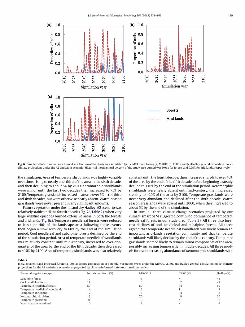

J.E. Halofsky et al. / Ecological Modelling 266 (2013) 131– 143 139

F d by thc nt of t

toaw2ag

rlattpowqt

TIp

ig. 6. Simulated future annual area burned as a fraction of the study area simulatelimate projections under the A2 emissions scenario. Historical mean annual perce

he simulation. Area of temperate shrublands was highly variablever time, rising to nearly one-third of the area in the sixth decade,nd then declining to about 5% by 2100. Xeromorphic shrublandsere minor until the last two decades then increased to >5% by

100. Temperate grasslands increased in area to over 5% in the thirdnd sixth decades, but were otherwise nearly absent. Warm-seasonrasslands were never present in any significant amounts.

Future vegetation under the hot and dry Hadley-A2 scenario waselatively stable until the fourth decade (Fig. 7c, Table 2), when veryarge wildfire episodes burned extensive areas in both the forestsnd arid lands (Fig. 6c). Temperate needleleaf forests were reducedo less than 40% of the landscape area following those events,hen began a slow recovery to 60% by the end of the simulationeriod. Cool needleleaf and subalpine forests declined by the end

f the simulation period. Area of temperate needleleaf woodlandsas relatively constant until mid-century, increased to over one-

uarter of the area by the end of the fifth decade, then decreasedo <10% by 2100. Area of temperate shrublands was also relatively

able 2nitial (current) and projected future (2100) landscape composition of potential vegetatrojections for the A2 emissions scenario, as projected by climate-informed state-and-tra

Potential vegetation type Initial conditions (%)

Subalpine forest 2

Cool needleleaf forest 11

Temperate needleleaf forest 59

Temperate needleleaf woodland 14

Temperate shrubland 12

Xeromorphic shrubland 2

Temperate grassland <1

Warm-season grassland 0

e MC1 model using (a) MIROC, (b) CSIRO, and (c) Hadley general circulation modelhe study area burned was 0.01% for forests and 0.09% for arid lands, respectively.

constant until the fourth decade, then increased sharply to over 40%of the area by the end of the fifth decade before beginning a steadydecline to <10% by the end of the simulation period. Xeromorphicshrublands were nearly absent until mid-century, then increasedsteadily to >20% of the area by 2100. Temperate grasslands werenever very abundant and declined after the sixth decade. Warmseason grasslands were absent until 2060, when they increased toabout 5% by the end of the simulation.

In sum, all three climate change scenarios projected by ourclimate smart STM suggested continued dominance of temperateneedleleaf forests in our study area (Table 2). All three also fore-cast declines of cool needleleaf and subalpine forests. All threeagreed that temperate needleleaf woodlands will likely remain animportant arid-lands vegetation community and that temperate

shrublands will likely decline by the end of the century. Temperategrasslands seemed likely to remain minor components of the area,possibly increasing temporarily in middle decades. All three mod-els forecast increasing abundance of xeromorphic shrublands with

ion types under the MIROC, CSIRO, and Hadley general circulation model climatensition models.

MIROC (%) CSIRO (%) Hadley (%)

<1 <1 <13 2 <1

59 74 6013 11 7

3 4 820 9 20

0 <1 01 <1 4

140 J.E. Halofsky et al. / Ecological Modelling 266 (2013) 131– 143

F otentm an of

ttcnwstais

4

Mi(aestdsd

ig. 7. Climate-informed state-and-transition model simulation of potential future podel climate projections under the A2 emissions scenario. Lines represent the me

he hot and dry Hadley-A2 scenario showing that they may becomehe dominant arid-land vegetation community by the end of theentury. The Hadley-A2, and to a lesser extent the MIROC-A2, sce-arios suggest increasing abundance of warm-season grasslands,hich are currently not present. Overall, linked DGVM-STM model

imulations under these three climate scenarios suggest that, athe end of the century, central Oregon will have a landscape witht least half its area in ponderosa pine forests and arid lands dom-nated by either temperate needleleaf woodlands or xeromorphichrublands, with reduced area of temperate shrublands.

. Discussion

We have shown how projections of vegetation shifts from theC1 DGVM (Fig. 5) differ from those produced by a climate-

nformed STM (Fig. 7). For example, the climate-informed STMFig. 7) showed much less variability in the extent of temper-te needleleaf forest (associated with ponderosa pine forest inastern OR) during the 21st century than MC1 (Fig. 5). Includingpecies-specific fire resistance and realistic constraints on vegeta-

ion change owing to the legacy of existing vegetation in the STMampens, in a biologically correct way, the frequency of vegetationhifts and results in greater vegetation resilience. On-going DGVMevelopment includes defining new plant functional types based

ial vegetation type trends for (a) MIROC, (b) CSIRO, and (c) Hadley general circulation30 Monte Carlo simulations for each climate scenario.

on physiological traits such as fire sensitivity. However physiolog-ical traits are still restricted to a handful of species, challengingthe DGVM modelers to make their improvements relevant at largescales.

Despite dampening year-to-year fluctuations by using 10-yearaverage climate (a 10-year period was used in this version ofthe model but could be modified to represent a longer interval),vegetation types in MC1 fluctuate sharply as climate conditionsevolve. The model does not simulate realistically long lags betweenchanges in environmental conditions and the actual replacement ofthe existing vegetation. This is particularly true on the West coastof the USA and the Pacific Northwest, where trees have survived forcenturies despite changing climates. STMs are specifically parame-terized to include empirically-defined successional trajectories thatlast decades to centuries unless a stand-replacement disturbancetriggers a switch to a different PVT. These ecological constraints onvegetation type change are predicated on the theory that disturb-ance will be the catalyst for vegetation shifts with changing climate(Littell et al., 2010). Furthermore, STMs incorporate species-specificresistance to disturbance that DGVMs cannot express, since they do

not simulate species. For example, with increased fire frequencyin STMs, more landscape area moves into an open, large-diameterponderosa pine state. Because ponderosa pine trees are very resis-tant to fire (Agee, 1993), fire does not frequently result in a state

l Mod

cmioSv

ltWbpwSricoabpmwPnbd

cbttptaaihifc

icepitoWtt

lfieawsrNwf

a

J.E. Halofsky et al. / Ecologica

hange when it occurs in the open, large-diameter pine state. Thus,uch of the area in the open, large-diameter pine state remains

n that state in STM simulations. In this way, ecological constraintsn vegetation type change and resistance to disturbance built intoTMs can produce decade- to century-long lags in climate-inducedegetation shifts.

Climate-informed STM simulations did not show some shrub-ands and grasslands being as resistant to climate change ashe DGVM. For example, temperate shrublands, associated with

yoming big sage in central Oregon, declined to a greater degreey 2100 in the STM simulations than in the MC1 simulations. Tem-erate grasslands that could be identified locally as Bluebunchheatgrass–Sandberg bluegrass were more abundant in MC1 than

TM simulations. This was also likely due to the species-specificesistance to disturbance (or lack thereof) that was built empir-cally into STMs. Species that comprise shrubland and grasslandommunities in central Oregon are generally not as fire resistantr long-lived as many of the tree species in dry forest types; thebove-ground portions of grasses and shrubs are generally killedy fire, and they recolonize via sprouting and stored or dispersedropagules. Thus, when a fire (even low-severity fire) occurs, com-unities shift to early-successional or open condition states, athich point available resources and lack of competition facilitate

VT shifts. Thus, we might expect similar landscapes dominatedow and in the future by shrublands and grasslands to be less sta-le than fire-resistant dry forests, unless pest outbreaks decimaterought-stressed forests.

Although episodic shifts in vegetation were dampened inlimate-informed STMs, results suggested that while there maye relative stability in vegetation conditions during the first threeo four decades of the 21st century, higher volatility in vegeta-ion conditions may occur mid-century, and stabilize again to lessroductive drought-adapted communities late in the 21st cen-ury. This might mean that habitat for species of interest and

variety of ecosystem services will appear relatively stable for few decades, then experience wide swings during the follow-ng decades, a future reminiscent of the green-up/brown-downypothesis whereby warming would first cause higher productivity

n energy- (temperature) limited systems that would soon after suf-er from drought conditions as warming continued and eventuallyaused widespread mortality.

Projected shifts in fire regimes and vegetation by climate-nformed STMs are generally consistent with other projections oflimate-induced change in the study region and elsewhere. Forxample, statistical models developed by McKenzie et al. (2004)rojected that the extent of the area burned by wildfires would

ncrease by a factor of 1.4–5 for most western states with a meanemperature increase of 2 ◦C. Similarly, statistical models devel-ped by Littell et al. (2010) for the eastern Cascades in Oregon andashington suggested that fire area burned will double or triple by

he 2080s. MC1 has projected such increases at various scales overhe region (Lenihan et al., 2008b; Rogers et al., 2011).

The decline in the extent of cool needleleaf forests in our simu-ations is consistent with a study by Littell et al. (2010) using datarom Rehfeldt et al. (2006), which showed a potential decreasen the areas of climatically suitable habitat for Douglas-fir in theastern Cascades of Washington. Douglas-fir is limited by watervailability during summer at lower elevations in the Pacific North-est (Littell et al., 2008). Increasing temperatures, lower winter

nowpack, and early snowmelt with climate change will likelyesult in decreased summer soil moisture in parts of the Pacificorthwest (Elsner et al., 2010). Decreased summer soil moisture

ill likely lead to a loss of climatically suitable habitat for mesic

orest types dominated by Douglas-fir east of the Cascade crest.The continued dominance of ponderosa pine forests in the study

rea is consistent with a study by Coops et al. (2005) who projected

elling 266 (2013) 131– 143 141

the expansion of ponderosa pine on the east side of the CascadeMountains using the 3-PG model. In contrast, Rehfeldt et al. (2006)projected decreases in the area of climatically suitable habitat forponderosa pine in the study area. However, the climate envelopemodeling approach used by Rehfeldt et al. (2006) omitted severalimportant factors addressed by our linked model approach, includ-ing fire dependency, CO2 fertilization effects, and biotic feedbacks.

4.1. Limitations to our approach

Our approach has several limitations:

• We have assumed that wildfire suppression will remain as effec-tive in the future as it is currently. However, extreme fire weathermay become more frequent with climate change (Abatzoglou andBrown, 2011) such that fire frequency and size may exceed ourassumptions.

• The MC1 version we used for this project did not include insectoutbreaks. STMs do incorporate insect outbreaks, but parametersare based on empirical data from past outbreaks, assuming sim-ilar conditions in the future. STMs could accommodate changesin the occurrence and intensity of insect or other disturbances ifestimates of potential changes in future disturbance frequencyand severity were readily available. On-going research in themodeling community to simulate insect population dynamicsand climate-driven outbreaks will likely provide such informa-tion in the near future.

• In the STMs, we restricted PVT changes to instances when vege-tation is in an early-successional or open condition or there is astand-replacement disturbance. Thus, we did not account for PVTshifts that may occur following mixed-severity disturbances.

• We did not build in lag times for species migration in theSTMs. Paleoecological records indicate that migration rates fortree species could be approximated to 200–300 m yr−1, with alarge associated uncertainty and species-specific response lags(Fischlin et al., 2007). We restricted all PVCs projected to occurin the three climate futures examined in this study to those thatcurrently exist in or near to our study area, making incorporationof migration lags in the models less critical.

• We have assumed that the known dynamics of plant communitiesand PVTs will be relevant in the future under different climaticconditions. However, vegetation growth rates, succession rates,and species interactions are likely to change in the future.

• To link MC1 with our STMs, we in some cases represented sev-eral PVTs with a single STM, thus resulting in loss of ecologicaldetail. This loss of ecological detail may have resulted in us miss-ing important PVT-specific responses to changes in climate anddisturbance.

Despite these limitations, results from climate-informed STMscan help to better understand potential interactions betweenregional-scale climate drivers, fine-scale vegetation dynamics, andshifts in disturbance regimes. Our results illustrated that legacyeffects incorporated in our STM confer resilience to some plantcommunities under changing climate. However, results also sug-gested that vegetation could appear to be stable in the early partof the 21st century, then shift rapidly with increased fire andaltered environmental conditions. Managers, in collaboration withscientists, can use output from this linked model process to con-sider potential climate-induced shifts in local vegetation conditionsand develop management actions that could minimize unwantedeffects of climate change. For example, in central Oregon, climate-

informed STM results showed that dry ponderosa pine forests arelikely to remain dominant across the landscape, but moist foreststhat are currently providing habitat for the northern spotted owlwill likely decline. Such results can provide a base of information

1 l Mod

fplricwi

A

tIAPNWh

R

A

A

A

A

A

B

B

B

C

C

C

C

D

D

D

E

E

42 J.E. Halofsky et al. / Ecologica

or interactions between scientists and managers to strategicallylan adaptive management actions (e.g., increase connectivity of

ate-successional forests for northern spotted owl). A forthcomingesearch effort will involve running different management scenar-os (developed through scientist-manager collaborations) in ourlimate-informed STM to determine what management activities inhat locations will likely maximize desirable vegetation conditions

n the central Oregon study area under a changing climate.

cknowledgments

This work was funded by the Western Wildland Environmen-al Threat Assessment Center, and was conducted as a part of thentegrated Landscape Assessment Project, which was funded by themerican Recovery and Reinvestment Act, the USDA Forest Serviceacific Northwest Research Station, the USDA Forest Service Pacificorthwest Region, and the USDA Forest Service Southwest Region.e thank Crystal Raymond and two anonymous reviewers for their

elpful suggestions to improve the manuscript.

eferences

batzoglou, J.T., Brown, T.J., 2011. A comparison of statistical downscaling meth-ods suited for wildfire applications. International Journal of Climatology 32,772–780.

gee, J.K., 1993. Fire Ecology of Pacific Northwest Forests. Island Press, Washington,DC.

llen, C.D., Macalady, A.K., Chenchouni, H., Bachelet, D., McDowell, N., Vennetier, M.,Kitzberger, T., Rigling, A., Breshears, D.D., Hogg, E.H., Gonzalez, P., Fensham, R.,Zhang, Z., Castro, J., Demidova, N., Lim, J., Allard, G., Running, S.W., Semerci, A.,Cobb, N., 2010. A global overview of drought and heat-induced tree mortalityreveals emerging climate change risks for forests. Forest Ecology and Manage-ment 259, 660–684.

nderson, G.K., Ottmar, R.D., Prichard, S.J., 2005. CONSUME 3.0 User’s Guide. USDAForest Service, Pacific Northwest Research Station, Seattle, WA.

pexRMS, ESSA, 2011. Path Landscape Model Online Documentation. Apex ResourceManagement Solutions Ltd. and ESSA Technologies Ltd., Ottawa, ON. Availableat: 〈http://wiki.pathmodel.com〉.

achelet, D., Lenihan, J.M., Daly, C., Neilson, R.P., 2000. Interactions between fire,grazing and climate change at Wind Cave National Park, SD. Ecological Modelling134, 229–244.

achelet, D., Lenihan, J.M., Daly, C., Neilson, R.P., Ojima, D.S., Parton, W.J., 2001. MC1,A Dynamic Vegetation Model for Estimating the Distribution of Vegetation andAssociated Carbon and Nutrient Fluxes, Technical Documentation Version 1.0.General Technical Report PNW-GTR-508. USDA Forest Service, Pacific NorthwestStation, Portland, OR.

achelet, D., Neilson, R.P., Hickler, T., Drapek, R.J., Lenihan, J.M., Sykes, M.T., Smith,B., Sitch, S., Thonicke, K., 2003. Simulating past and future dynamics of naturalecosystems in the United States. Global Biogeochemical Cycles 17, 1045.

ohen, J.D., Deeming, J.E., 1985. The National Fire-Danger Rating System: BasicEquations. General Technical Report PSW-GTR-82. USDA Forest Service PacificSouthwest Research Station, Berkeley, CA.

oops, N.C., Waring, R.H., Law, B.E., 2005. Assessing the past and future distributionand productivity of ponderosa pine in the Pacific Northwest using a processmodel, 3-PG. Ecological Modelling 183, 107–124.

ramer, W., Bondeau, A., Woodward, F.I., Prentice, E., Betts, R.A., Brovkin, V., Cox,P.M., Fisher, V., Foley, J.A., Friend, A.D., Kucharik, C., Lomas, M.R., Ramankutty,N., Sitch, S., Smith, B., White, A., Young-Molling, C., 2001. Global responseof terrestrial ecosystem structure and function to CO2 and climate change:results from six global dynamic vegetation models. Global Change Biology 7,357–373.

rookston, N.L., Finley, A.O., 2007. yaImpute: an R package for k-NN imputation.Journal of Statistical Software 23, 1–16.

aly, C., Bachelet, D., Lenihan, J.M., Neilson, R.P., Parton, W., Ojima, D., 2000. Dynamicsimulation of tree–grass interactions for global change studies. Ecological Appli-cations 10, 449–469.

aly, C., Halbleib, M., Smith, J.I., Gibson, W.P., Doggett, M.K., Taylor, G.H., Curtis, J.,Pasteris, P.P., 2008. Physiographically sensitive mapping of climatological tem-perature and precipitation across the conterminous United States. InternationalJournal of Climatology 28, 2031–2064.

aly, C., Taylor, G.H., Gibson, W.P., 1997. The PRISM approach to mapping precip-itation and temperature. In: Proceedings of the 10th American MeteorologicalSociety Conference on Applied Climatology. American Meteorological Society,Reno, NV, pp. 10–12.

idenshink, J., Schwind, B., Brewer, K., Zhu, Z.L., Quayle, B., Howard, S., 2007. A projectfor monitoring trends in burn severity. Fire Ecology 3, 3–20.

lsner, M.M., Cuo, L., Voisin, N., Deems, J.S., Hamlet, A.F., Vano, J.A., Mickelson, K.E.B.,Lee, S., Lettenmaier, D.P., 2010. Implications of 21st century climate change forthe hydrology of Washington State. Climatic Change 102, 225–260.

elling 266 (2013) 131– 143

ESSA Technologies Ltd., 2007. Vegetation Dynamics Development Tool User Guide,Version 6.0. Vancouver, British Columbia.

Evers, L., 2010. Modeling Sage-grouse Habitat Using a State-and-Transition Model.Ph.D. Dissertation. Oregon State University, Corvallis, OR.

Fischlin, A., Midgley, G.F., Price, J.T., Leemans, R., Gopal, B., Turley, C., Rounsevell,M.D.A., Dube, O.P., Tarazona, J., Velichko, A.A., 2007. Ecosystems, their proper-ties, goods, and services. In: Parry, M.L., Canziani, O.F., Palutikof, J.P., van derLinden, P.J., Hanson, C.E. (Eds.), Climate Change: Impacts, Adaptation, and Vul-nerability: Contribution of Working Group II to the Fourth Assessment Reportof the Intergovernmental Panel on Climate Change. Cambridge University Press,Cambridge, UK, pp. 211–272.

Foley, J.A., Levis, S., Prentice, I.C., Pollard, D., Thompson, S.L., 1998. Coupling dynamicmodels of climate and vegetation. Global Change Biology 4, 561–579.

Forbis, T.A., Provencher, L., Frid, L., Medlyn, G., 2006. Great Basin land managementplanning using ecological modeling. Environmental Management 38, 62–83.

Fowler, H.J., Blenkinsop, S., Tebaldi, C., 2007. Linking climate change modeling toimpacts studies: recent advances in downscaling techniques for hydrologicalmodeling. International Journal of Climatology 27, 1547–1578.

Friedlingstein, P., Fung, I., Holland, E., John, J., Brasseur, G., Erickson, D., Schimel, D.,1995. On the contribution of CO2 fertilization to the missing biospheric sink.Global Biogeochemical Cycles 9, 541–556.

Gonzalez, P., Neilson, R.P., Lenihan, J.M., Drapek, R.J., 2010. Global patterns in thevulnerability of ecosystems to vegetation shifts due to climate change. GlobalEcology and Biogeography 19, 755–768.

Gordon, C., Cooper, C., Senior, C.A., Banks, H.T., Gregory, J.M., Johns, T.C., Mitchell,J.F.B., Wood, R.A., 2000. The simulation of SST, sea ice extents and ocean heattransports in a version of the Hadley Centre coupled model without flux adjust-ments. Climate Dynamics 16, 147–168.

Gordon, H.B., Rotstayn, L.D., McGregor, J.L., Dix, M.R., Kowalczyk, E.A., Farrell, S.P.,Waterman, L.J., Hirst, A.C., Wilson, S.G., Collier, M.A., Watterson, I.G., Elliott,T.I., 2002. The CSIRO Mk3 Climate System Model. CSIRO Atmospheric ResearchTechnical Paper No. 60. CSIRO Atmospheric Research.

Halofsky, J.E., Peterson, D.L., O’Halloran, K.A., Hawkins Hoffman, C. (Eds.), 2011.Adapting to Climate Change at Olympic National Forest and Olympic NationalPark. General Technical Report PNW-GTR-844. USDA Forest Service, PacificNorthwest Research Station, Portland, OR.

Hann, W.J., Jones, J.L., Karl, M.G., Hessburg, P.F., Keane, R.E., Long, D.G., Menakis,J.P., McNicoll, C.H., Leonard, S.G., Gravenmier, R.A., Smith, B.G., 1997. Land-scape Dynamics of The Basin. In: Quigley, T.M., Arbelbide, S.J. (Eds.), AnAssessment of Ecosystem Components in the Interior Columbia Basin andPortions of the Klamath and Great Basins. General Technical Report PNW-GTR-405. USDA Forest Service, Pacific Northwest Research Station, Portland, OR,pp. 337–1055.

Hasumi, H., Emori, S. (Eds.), 2004. K-1 Coupled Model (MIROC) Description. TechnicalReport 1. University of Tokyo, Center for Climate System Research, Tokyo.

Hayhoe, K., Cayan, D., Field, C., Frumhoff, P., Maurer, E., Miller, N., Moser, S., Schnei-der, S., Cahill, K., Cleland, E., Dale, L., Drapek, R., Hanemann, R., Kalkstein, L.,Lenihan, J., Lunch, C., Neilson, R., Sheridan, S., Verville, J., 2005. Emission path-ways, climate change, and impacts on California. Proceedings of the NationalAcademy of Sciences 101, 12422–12427.

Hemstrom, M.A., Korol, J.J., Hann, W.J., 2001. Trends in terrestrial plant communitiesand landscape health indicate the effects of alternative management strate-gies in the interior Columbia River basin. Forest Ecology and Management 153,105–125.

Hemstrom, M.A., Merzenich, J., Reger, A., Wales, B., 2007. Integrated analysis of land-scape management scenarios using state and transition models in the upperGrande Ronde River Subbasin, Oregon, USA. Landscape and Urban Planning 80,198–211.

Hemstrom, M.A., Wisdom, M.J., Hann, W.J., Rowland, M.M., Wales, B.C., Gravenmier,R.A., 2002. Sagebrush-steppe vegetation dynamics and restoration potential inthe Interior Columbia Basin, U.S.A. Conservation Biology 16, 1243–1255.

Hickler, T., Smith, B., Sykes, M.T., Davis, M.B., Sugita, S., Walker, K., 2004. Using ageneralized vegetation model to simulate vegetation dynamics in northeasternUSA. Ecology 85, 519–530.

Horn, H.S., 1975. Markovian properties of forest succession. In: Cody, M.L., Diamond,J.M. (Eds.), Ecology and Evolution of Communities. Harvard University Press,Cambridge, MA, pp. 196–211.

IPCC [Intergovernmental Panel on Climate Change], 2007. In: Solomon, S., Qin, D.,Manning, M., Chen, Z., Marquis, M., Avery, K.B., Tignor, M., Miller, H.L. (Eds.),Contribution of Working Group I to the Fourth Assessment Report of the Inter-governmental Panel on Climate Change. Cambridge University Press, Cambridgeand New York.

Johns, T.C., Gregory, J.M., Ingram, W.J., Johnson, C.E., Jones, A., Lowe, J.A., Mitchell,J.F.B., Roberts, D.L., Sexton, D.M.H., Stevenson, D.S., Tett, S.F.B., Woddage, M.J.,2003. Anthropogenic climate change for 1860 to 2100 simulated with theHadCM3 model under updated emissions scenarios. Climate Dynamics 20,583–612.

Laycock, W.A., 1991. Stable states and thresholds of range condition on North Amer-ican rangelands: a viewpoint. Journal of Range Management 44, 427–433.

Lenihan, J.M., Bachelet, D., Neilson, R.P., Drapek, R., 2008a. Response of vegetationdistribution, ecosystem productivity, and fire to climate change scenarios for

California. Climatic Change 87 (Suppl 1), S215–S230.

Lenihan, J.M., Bachelet, D., Neilson, R.P., Drapek, R.J., 2008b. Simulated response ofconterminous United States ecosystems to climate change at different levels offire suppression, CO2 emission rate, and growth response to CO2. Global andPlanetary Change 64, 16–25.

l Mod

L

L

L

L

M

M

M

M

N

N

N

O

O

P

P

J.E. Halofsky et al. / Ecologica

enihan, J.M., Daly, C., Bachelet, D., Neilson, R.P., 1998. Simulating broad-scale fireseverity in a dynamic global vegetation model. Northwest Science 72, 91–103.

enihan, J.M., Drapek, R.J., Bachelet, D., Neilson, R.P., 2003. Climate changes effectson vegetation distribution, carbon, and fire in California. Ecological Applications13, 1667–1681.

ittell, J.S., Oneil, E.E., McKenzie, D., Hicke, J.A., Lutz, J.A., Norheim, R.A., Elsner, M.M.,2010. Forest ecosystems, disturbance, and climatic change in Washington State,USA. Climatic Change 102, 129–158.

ittell, J.S., Peterson, D.L., Tjoelker, M., 2008. Douglas-fir growth in mountain ecosys-tems: water limits tree growth from stand to region. Ecological Monographs 78,349–368.

cKenzie, D.H., Gedalof, Z., Peterson, D.L., Mote, P., 2004. Climatic change, wildfire,and conservation. Conservation Biology 18, 890–902.

erzenich, J., Kurz, W.A., Beukema, S., Arbaugh, M., Schilling, S., 2003. Determin-ing forest fuel treatments for the Bitterroot front using VDDT. In: Arthaud, G.J.,Barrett, T.M. (Eds.), Systems Analysis in Forest Resources. Kluwer AcademicPublishers, Dordrecht, pp. 47–59.

itchell, T.D., Carter, T.R., Jones, P.D., Hulme, M., New, M., 2004. A ComprehensiveSet of High-Resolution Grids of Monthly Climate for Europe and the Globe: TheObserved Record (1901–2000) and 16 Scenarios (2001–2100). University of EastAnglia, Norwich, UK.

ote, P.W., Salathé Jr., E.P., 2010. Future climate in the Pacific Northwest. ClimaticChange 102, 29–50.

akicenovic, N., Swart, R. (Eds.), 2000. Special Report on Emissions Scenarios. ASpecial Report of Working Group III of the Intergovernmental Panel on ClimateChange. Cambridge University Press, Cambridge and New York.

eilson, R.P., 1995. A model for predicting continental-scale vegetation distributionand water balance. Ecological Applications 5, 362–385.

oble, I.R., Slatyer, R.O., 1980. The use of vital attributes to predict successionalchanges in plant communities subject to recurrent disturbances. Vegetatio 43,5–21.

hmann, J., Gregory, M.J., 2002. Predictive mapping of forest composition and struc-ture with direct gradient analysis and nearest neighbor imputation in coastal OR,USA. Canadian Journal of Forest Research 32, 725–741.

mernik, J.M., 1987. Ecoregions of the coterminous United States. Annals of theAssociation of American Geographers 77, 118–125.

armesan, C., 2006. Ecological and evolutionary responses to recent climate change.Annual Review of Ecology, Evolution, and Systematics 37, 637–669.

arton, W.J., Scurlock, J.M.O., Ojima, D.S., Gilmanov, T.G., Scholes, R.J., Schimel, D.S.,Kirchner, T., Menaut, J.C., Seastedt, T., Garcia Moya, E., Kamnalrut, A., Kinya-mario, J.I., 1993. Observations and modeling of biomass and soil organic matterdynamics for the grassland biome worldwide. Global Biogeochemical Cycles 7,785–809.

elling 266 (2013) 131– 143 143

Peterson, D.L., Ryan, K.C., 1986. Modeling postfire conifer mortality for long-rangeplanning. Environmental Management 10, 797–808.

Prentice, I.C., Bondeau, A., Cramer, W., Harrison, S., Hickler, T., Lucht, W., Sitch, S.,Smith, B., Sykes, M., 2007. Dynamic global vegetation modeling: quantifyingterrestrial ecosystem responses to large-scale environmental change. In:Canadell, J.G., Pataki, D., Pitelka, L.F. (Eds.), Terrestrial Ecosystems in a ChangingWorld. Springer-Verlag, Berlin, pp. 175–192.

Prentice, I.C., Webb, R.S., Ter-Mikhaelian, M.T., Solomon, A.M., Smith, T.M., Pitovra-nov, S.E., Nikolov, N.T., Minin, A.A., Leemans, R., Lavorel, S., Korzukhin, M.D.,Helmisaari, H.O., Hrabovszky, J.P., Harrison, S.P., Emanuel, W.R., Bonan, G.B.,1989. Developing a Global Vegetation Dynamics Model: Results of an IIASA Sum-mer Workshop. Research Report RR-89-7. International Institute for AppliedSystems Analysis, Laxenburg.

PRISM Group, 2012. Parameter-elevation Regressions on Independent Slopes ModelClimate Mapping System. Available at: http://www.prism.oregonstate.edu/

Provencher, L., Anderson, T., 2011. Climate Change Revisions to Nevada’s WildlifeAction Plan: Vegetation Mapping and Modeling Report to the Nevada Depart-ment of Wildlife. The Nature Conservancy, Reno, NV.

Rehfeldt, G.E., Crookston, N.L., Warwell, M.V., Evans, J.S., 2006. Empirical analysis ofplant-climate relationships for the western United States. International Journalof Plant Sciences 167, 1123–1150.

Rogers, B.M., Neilson, R.P., Drapek, R., Lenihan, J.M., Wells, J.R., Bachelet, D., Law, B.E.,2011. Impacts of climate change on fire regimes and carbon stocks of the U.S.Pacific Northwest. Journal of Geophysical Research 116, G03037.

Rothermel, R., 1972. A Mathematical Model for Fire Spread Predictions in WildlandFuels: Research Paper INT-RP-115. USDA Forest Service, Ogden, UT.

Shaw, M.R., Pendleton, L., Cameron, D.R., Morris, B., Bachelet, D., Klausmeyer, K.,MacKenzie, J., Conklin, D.R., Bratman, G.N., Lenihan, J., Haunreiter, E., Daly, C.,Roehrdanz, P.R., 2011. The impact of climate change on California’s ecosystemservices. Climatic Change 109 (Suppl 1), S465–S484.

The Nature Conservancy, USDA Forest Service, and Department of the Interior,2006. LANDFIRE Vegetation Dynamics Modeling Manual, Version 4.1. Boulder,CO.

van Wagner, C.E., 1973. Height of crown scorch in forest fires. Canadian Journal ofForest Research 3, 373–378.

Weisz, R., Triepke, J., Truman, R., 2009. Evaluating the ecological sustainability ofa ponderosa pine ecosystem on the Kaibab Plateau in northern Arizona. FireEcology 5, 100–114.

Westerling, A.L., Hidalgo, H.G., Cayan, D.R., Swetnam, T.W., 2006. Warming andearlier spring increase western U.S. forest wildfire activity. Science 313,940–943.

Westoby, M., Walker, B., Noy-Meir, I., 1989. Opportunistic management for range-lands not at equilibrium. Journal of Range Management 42, 266–276.