ASSESSING POLICIES FOR REDUCING GREENHOUSE GAS EMISSIONS FROM PASSENGER VEHICLES

Jillian Mallory BSc.Eng, University of New Brunswick, 2000

RESEARCH PROJECT SUBMITTED IN PARTIAL FULFILLMENT OF THE REQUIREMENTS FOR THE DEGREE OF

MASTER OF RESOURCE MANAGEMENT

In the School of Resource and Environmental Management

of Simon Fraser University

0 Jillian Mallory, 2007

SIMON FRASER UNIVERSITY

Fall 2007

All rights reserved. This work may not be reproduced in whole or in part, by photocopy

or other means, without permission of the author.

APPROVAL

Name:

Degree:

Jillian Mallory

Master of Resource Management

Report No.: 437

Title of Research Project: Assessing Policies for Reducing Greenhouse Gas Emissions from Passenger Vehicles

Examining Committee:

Chair: Bill Tubbs

Date Approved:

MarkJaccard Senior Supervisor Professor, School of Resource and Environmental Management Simon Fraser University

Nic Rivers Supervisor Research Associate, Ph.D Candidate, School of Resource and Environmental Management Simon Fraser University

Declaration of Partial Copyright Licence

The author, whose copyright is declared on the title page of this work, has granted to Simon Fraser University the right to lend this thesis, project or extended essay to users of the Simon Fraser University Library, and to make partial or single copies only for such users or in response to a request from the library of any other university, or other educational institution, on its own behalf or for one of its users.

The author has further granted permission to Simon Fraser University to keep or make a digital copy for use in its circulating collection (currently available to the public at the "Institutional Repository" link of the SFU Library website <www.lib.sfu.ca> at: ~http:Nir.lib.sfu.calhandlell8921112~) and, without changing the content, to translate the thesislproject or extended essays, if technically possible, to any medium or format for the purpose of preservation of the digital work.

The author has further agreed that permission for multiple copying of this work for scholarly purposes may be granted by either the author or the Dean of Graduate Studies.

It is understood that copying or publication of this work for financial gain shall not be allowed without the author's written permission.

Permission for public performance, or limited permission for private scholarly use, of any multimedia materials forming part of this work, may have been granted by the author. This information may be found on the separately catalogued multimedia material and in the signed Partial Copyright Licence.

While licensing SFU to permit the above uses, the author retains copyright in the thesis, project or extended essays, including the right to change the work for subsequent purposes, including editing and publishing the work in whole or in part, and licensing other parties, as the author may desire.

The original Partial Copyright Licence attesting to these terms, and signed by this author, may be found in the original bound copy of this work, retained in the Simon Fraser University Archive.

Simon Fraser University Library Burnaby, BC, Canada

Revised: Fall 2007

ABSTRACT

Passenger vehicles are a large and growing source of greenhouse gas (GHG)

emissions. Policies aimed at inducing technological change in vehicles will liltely

contribute to curbing emissions. A hybrid energy-economy model of the passenger

vehicle sector was built to evaluate policies in reducing emissions, and in particular,

increasing the adoption of zero-emission vehicles (ZEVs). The model is technologically

explicit, behaviourally realistic and incorporates drivers of technological change. It was

applied to California to assess a tax on GHG emissions, a standard mandating ZEV

adoption, a ZEV purchase subsidy and a research and development subsidy for ZEVs.

Combinations of these policies were also examined. A standard combined with a tax

was found to most cost-effectively reduce emissions and increase ZEV diffusion. The

purchase subsidy was least cost-effective. More moderate emission reductions can be

achieved with diffusion of ultra low-emission vehicles, but deep reductions will likely

require adoption of zero-emission vehicles.

Keywords: technological change; zero-emission vehicles; hybrid model; climate change policy; transportation model; uncertainty

Subject Terms: Transportation, Automotive -- Environmental aspects; Technological innovations -- Environmental aspects; Climatic changes -- Government policy; Climatic changes -- Economic aspects; Environmental policy -- Economic aspects; Climatic changes -- Mathematical models

ACKNOWLEDGEMENTS

I would like to thank Mark Jaccard for providing both vision and inspiration in my

beginning and completing this project. I valued Mark's leadership and enthusiasm

throughout this project. Nic Rivers offered assistance throughout this research on many

levels. I thank Nic for his exceptional input as well as his endless encouragement. I

thank all the members of the Energy and Materials Research Group, particularly Jotham

Peters for sharing his extensive knowledge of economic costing, as well as Jonn Axsen,

Bill Tubbs, Steve Groves and Katherine Muncaster for their valued input and support. I

also appreciate the insight Hadi Dowlatabadi provided at the beginning of this project.

I thank the National Science and Engineering Research Council of Canada, the British

Columbia Automobile Association, and the Canadian Lnstitute of Energy for funding

support.

Lastly, I thank Ian Bruce and my family for their encouragement and support throughout

the completion of this project.

TABLE OF CONTENTS . . Approval .......................................................................................................................... 11

... ............................................................................................................................. Abstract 111

Acknowledgements ......................................................................................................... iv

Table of Contents ............................................................................................................... v . . List of Figures ............................................................................................................... VII

... List of Tables .................................................................................................................. viii

List of Equations .............................................................................................................. ix

Abbreviations ..................................................................................................................... x

Chapter 1: Introduction and Background .......... ... ............ ..... ......................................... 1 1.1 Technological Change and Environmental Policy ................................................ 2

1.1.1 Technological Change. the Environment and the Potential for Policy ........... 2 1 . 1.2 Environmental Policies .................................................................................. 4

1.2 Technological Change in Light Duty Vehicles ..................................................... 8 1.2.1 Trends in the Light Duty Vehicle Sector ........................................................ 8 1.2.2 Status of Zero-Emission Vehicle Technologies ........................................... 10

1.3 Alternative Environmental and Technology Policies in Light Duty Vehicles ............................................................................................................... 14

1.3.1 Analysis of Light Duty Vehicle Sector Policies ........................................... 18 1.4 Study Scenario: The California Light Duty Vehicle Sector ............................... 19 1.5 Modelling Considerations .................................................................................... 21 1.6 Research Objectives ............................................................................................. 24

Chapter 2: Methods ......................................................................................................... 26 2.1 The Model ............................................................................................................ 26

2.1.1 Technology Competition .............................................................................. 27 2.1.2 Endogenous Technological Change ............................................................. 30

........................................................................................... 2.1.3 Feedback Effects 35 2.1.4 Summary of Model ....................................................................................... 36

............................................................................................. 2.2 Analysis of Policies 37 ................................................................................................. 2.2.1 Policy Target 38

2.2.2 Evaluating the Cost of Policy Measures ....................................................... 40 2.3 Input Assumptions and Application to California ............................................... 42

........................... 2.3.1 Demand Forecast and Vehicle Ownership Characteristics 42 2.3.2 Vehicle Technology Characteristics ............................................................. 43 2.3.3 Other Key Model Parameters ....................................................................... 49

.................................................................... 2.3.4 Fuel Costs and Characteristics 51 2.4 Policies Assessed ................................................................................................. 54

.................................................................................... 2.5 Incorporating Uncertainty 56

Chapter 3: Results and Discussion ................................................................................. 59 .................................................................................. 3.1 Business as Usual Forecast 59

............................................................................. 3.2 Results of Policy Comparison 62 ................................................................................................ 3.2.1 Policy Details 63

......................................................................... 3.2.2 Greenhouse Gas Emissions 66 .............................................................................................. 3.2.3 ZEV Diffusion 71

................................................... 3.2.4 Key Characteristics of Policy Alternatives 73 ......................................................................... 3.2.5 Costs of Policy Alternatives 76

.................................................................................... 3.2.6 Are ZEVs Required? 86 3.3 Single Parameter Sensitivity Analysis ................................................................. 88

........................... 3.3.1 Sensitivity of Cost Comparisons to Social Discount Rate 88 ....................................................... 3.3.2 Determining Key Uncertain Parameters 91

Chapter 4: Summary and Conclusions .......................................................................... 99 .............................................................................................................. 4.1 Summary 99

............................................ 4.2 Model Limitations and Areas for Future Research 103 .......................................................................... 4.2.1 Full-Equilibrium Analysis 103

............................................................................ 4.2.2 Firm-level representation 104 ................................................ 4.2.3 Further Policy Alternatives to be Assessed 106

.......................................................... 4.2.4 Treatment of Technological Change 107 ........................................................................................................ 4.3 Conclusions 108

Reference List ................................................................................................................. 110

LIST OF FIGURES

Figure 1 : Figure 2: Figure 3: Figure 4:

Figure 5:

Figure 6: Figure 7:

Figure 8: Figure 9: Figure 10: Figure 1 1: Figure 12: Figure 13 : Figure 14: Figure 15:

Figure 16: Figure 17:

Figure 18:

Figure 19: Figure 20: Figure 2 1 :

Figure 22: Figure 23: Figure 24: Figure 25:

Selected Policies within Spectrum of Compulsoriness .................................. 5 Light Duty Vehicle Competition .................................................................. 28 Diagram of California Light Duty Vehicle Sector Model ............................ 37 Declining Capital Cost (Single Factor Learning Curve) Battery Electric Cars ................................................................................................. 47 Declining Capital Cost (Two factor Learning Curve) Battery Electric Cars ................................................................................................. 47 Intangible Cost Curve for Battery Electric Cars .......................................... 49 Fuel Costs per GJ (2000 U.S.dollars) ........................................................... 52

Indirect Emissions Scenario ......................................................................... 54 BAU Emissions Forecast (Direct and Indirect Emissions) .......................... 60 BAU New Market Share Forecast ................................................................ 61 EIA Forecast ................................................................................................ 62 Direct GHG Emissions for Simulated Policies ............................................ 66 2045 GHG Emissions Levels .................................................................. 67 Cumulative Direct GHG Emissions ............................................................. 69 Breakdown of Cumulative GHG Emissions - Direct and Indirect Emissions .................................................................................................... -70 2045 ZEV New Market Share (%) ............................................................... 73

Cost of Policy Alternatives - discounted to 1990 at 3%/year, 2000 U.S dollars .................................................................................................... 78 Cost-Effectiveness of Policy Alternatives per tonne C 0 2 reduced - costs discounted to 1990 at 3%/year, 2000 U.S dollars ............................... 79

Median Costs by Discount Rate (2000 U.S. dollars) ................................. 82 Median Cost-effectiveness by Discount rate ($/tonne GHG reduced) ......... 83 Impact of R&D Investment on Discounted Costs of Policy - discounted at 3% .......................................................................................... 85

....................... Sensitivity of Median Policy Costs to Social Discount Rate 90 .............. Sensitivity of Median Cost-effectiveness to Social Discount Rate 90

Single Parameter Sensitivity -2045 C02e Emissions (Mt) ......................... 93 Single Parameter Sensitivity - Selected Policies 2045 ZEV New Market Share ................................................................................................ 96

vii

LIST OF TABLES

Table 1: Table 2:

Table 3: Table 4:

Table 5: Table 6: Table 7: Table 8:

Table 9: Table 10:

Vehicle Ownership Characteristics .............................................................. 43 Summary of Vehicle Characteristics for Cars .............................................. 46

Summary of Intangible Vehicle Characteristics for Cars ............................. 48

Other Key Model Parameters ...................................................................... 51 Direct Emission Factors ............................................................................... 52 Summary of Policies Assessed ..................................................................... 56 Policy Details ............................................................................................. 63 ZEV Diffusion in Policy Alternatives Tested .............................................. 71

Highlighted Characteristics of Policy Alternatives ...................................... 74 ULEV-ZEV Standard Compared with ZEV Standard and Standard plus tax ................................ .. .................................................................... 87

LIST OF EQUATIONS

......................................................................................................................... Equation 1 9 Equation 2 ......................................................................................................................... 28 Equation 3 ......................................................................................................................... 30

Equation 4 ......................................................................................................................... 31

Equation 5 .................................................................................................................... 32 Equation 6 ......................................................................................................................... 33

Equation 7 ......................................................................................................................... 33

Equation 8 .................................. .... ............................................................................. 35 Equation 9 ......................................................................................................................... 36

ABBREVIATIONS

AEEI

BAU

BEV

BPHEV

CARB

co2

C02e

ESUB

GHG

GJ

HEV

HFCV

IPCC

suv

ULEV

VMT

ZEV

Autonomous Energy Efficiency Index

Business as usual

Battery electric vehicle

Biofuel plug-in hybrid electric vehicle

California Air Resources Board

Carbon dioxide

Carbon dioxide equivalent

Elasticities of Substitution

Greenhouse gas

Gigajoule

Hybrid-electric vehicle

Hydrogen he1 cell vehicle

Intergovernmental Panel on Climate Change

Megatonnes

Research and development

Sport utility vehicle

Ultra-low emission vehicle

Zero-emission vehicle

CHAPTER 1: INTRODUCTION AND BACKGROUND

There is a near consensus among climate experts that anthropogenic greenhouse

gas emissions will have to be significantly constrained to stabilize their concentrations in

the atmosphere and thus prevent "dangerous interference" with the climate system. New

technology is often cited as a way to reconcile conflicts between the need to reduce

emissions and economic well-being. There is a particular interest for assessing how

various policies can stimulate the innovation and adoption of low or zero greenhouse gas

emitting technologies.

Light duty vehicles are a large and growing source of greenhouse gas emissions in

many jurisdictions.' Several new technologies hold promise for eliminating the

greenhouse gas emissions of cars and trucks. These so-called zero-emission technologies

are at an early stage in their development and diffusion, and policies to support their

innovation, demonstration and adoption may be warranted. However, there continues to

be debate surrounding which policy instruments would be best suited for this task.

In thls study, I analyzed several policies under a dual goal of reducing greenhouse

gas emissions and promoting the innovation and adoption of zero-emission vehicles. For

this analysis, I built a model of the passenger-vehicle transportation sector. The model

characterizes how consumers make decisions when purchasing a vehicle. Key features of

the process of technological development and adoption were included in the model. As a

I Light duty vehicles are generally characterized as passenger vehicles. In the U.S. they are defined as vehicles weighing less than 8,500 Ibs (Environmental Protection Agency [EPA], 2006a). In this study I use light duty vehicles and passenger vehicles interchangeably.

case study, I applied this model to California, comparing how various policies perform

based on this dual goal in California over the mid to long-term.

In the following chapter, I introduce a number of topics that are significant to this

study. First, I examine the connections between technology and environmental policy

and introduce various types of policy (Section 1.1). Second, I analyze trends in the light

duty vehicle sector and discuss why investigating policy to reduce emissions and

stimulate the innovation and adoption of new technologies in this sector is particularly

relevant (Section 1.2). Third, I identify a number of policies that are pertinent to the light

duty vehicle sector and summarize previous policy analyses targeted at this sector. This

informs the selection of policies which I assessed (Section 1.3). Fourth, I detail the

scenario under which selected policies were compared and describe why California

provides a good case study for this analysis (Section 1.4). Finally, I briefly discuss a

number of considerations in modelling the passenger vehicle sector (Section 1.5). I

conclude by summarizing and outlining my research objectives (Section 1.6).

1.1 Technological Change and Environmental Policy

1.1.1 Technological Change, the Environment and the Potential for Policy

Addressing climate change will require substantial efforts over a long timescale to

stabilize greenhouse gas emissions at what is considered an acceptable or "safe" level

(International Panel on Climate Change [IPCC], 2007). New technologies and processes

hold promise for resolving the inherent conflict between economic prosperity and our

desire for a stable climate system (Jaffe & Stavins, 1995). Through the adoption of new

technologies, we may benefit from the same or better goods and services while emitting

fewer greenhouse gases. For example, in the transportation sector, the adoption of hybrid

electric vehicles can lower greenhouse gas emissions while meeting the same consumer

demands for vehicle travel.

The discovery and use of new technologies and processes is referred to as

technological change. However, technological change is not simply a substitution of one

technology for another but is characterized by a number of stages (Grubler, Nakicenovic,

& Victor, 1999).~ Typically, when a technology is invented it is uncompetitive for two

reasons. First, the financial costs of the invented technology may be higher than

competing technologies. Second, the new technology may have some real or perceived

drawbacks that contribute to its non-competitiveness (Walls, 1996). For instance, the

consumer may perceive a loss of quality with the new technology or an increase in risk

because the technology lacks a record of past performance. These non-financial costs are

termed intangible costs.

R&D investments and demonstration projects can improve a new technology such

that the financial and intangible costs decline. These cost improvements allow the new

technology to become viable in small markets not addressed by existing products. Once

the technology is able to compete successfully in these so-called niche markets, its costs

are expected to further decline as cumulative experience with the technology increases

(Boston Consulting Group, 1968). This may lead to the standardization and mass

production of the technology, known as diffusion.

Uncertainty and non-linearities are prevalent in the process of technological change. For example, many technologies that are invented are not widely adopted. Further, related technologies have been observed to evolve in clusters, as the benefits of one technology are amplified by the adoption of a related technology (Grubler et al., 1999).

Technological change occurs naturally in markets and depending on its direction

and extent, technological change has the potential to both increase and decrease our

emissions. Increasingly, a pathway of technological change that lowers emissions

without changes in human activity is thought to be the "line of least resistance" for

reducing society's greenhouse gas emissions (Azar & Dowlatabadi, 1999). Thus,

policymakers are interested in influencing the direction of technological change by

promoting the innovation and adoption of less greenhouse gas intensive technologies.

Technological change stimulated through policy is known as induced technological

change (Goulder, 2004).

It is generally agreed that environmental policy can induce technological change

(for a review of the literature see Jaffe, Newell, & Stavins, 2002). However, much debate

remains on what kinds of policies are most likely to generate innovative, low-cost

solutions to environmental problems. In the following, I present commonly discussed

environmental policies.

1.1.2 Environmental Policies

One approach in categorizing environmental policy is in terms of a policy's

compulsoriness, or the extent to which certain behaviour is required by the government.

Within a range of compulsoriness, various policies and proposals employ an array of

incentives to induce technological change and reduce greenhouse gas emissions. Figure

1 shows where a selection of policies fall within this spectrum of compulsoriness. In the

following, I describe each of these policies, beginning with the most compulsory policies

and progressing to less compulsory policies.

Figure 1: Selected Policies within Spectrum of Compulsoriness

More Less Compulsory Compulsory

Spectrum of Compulsoriness 4 t

t

Command and Control policies Performance standards Technology standards

Market-based policies Emission taxes Purchase subsidies R&D subsidies

Cap and trade system Standard with credit trading

Conzmand-and-control regulations, such as performance and technology

standards, regulate specific emission levels or technologies which a firm or individual

must meet or adopt. These compulsory policies are enforced through financial or legal

penalties. These policies may create a viable market for targeted low-emission

technologies. Performance and technology standards can further induce technological

change by explicit "technology-forcing", which is mandating the use of technologies that

are in their early stages or not fully developed.

Technology-forcing standards are intended to exploit natural tendencies of

technological change by providing a market for new technologies regarded as

environmentally superior. A new technology may benefit from increased market share

by two means, learning-by-doing and the neighbour effect. Learning-by-doing describes

a phenomenon in which the financial costs of new technologies are observed to decline

with increases in cumulative experience with a technology (McDonald & Schrattenholzer,

2001). Further, as the market share of a technology increases, there is some evidence to

suggest that the intangible costs of a technology also decline. This observation, deemed

the neighbour effect, is attributed to factors such as consumers' increased perceptions of a

technology's reliability and learning from other consumers' experiences with the new

technology (Yang & Allerby, 2003).

Market basedpolicies, such as pollution taxes and subsidies, incite the firm or

consumer to take socially desirable actions simply by acting out of financial self-interest

(Stavins, 2001). Unlike command-and-control policies, firms and individuals decide how

much to reduce their emissions to avoid paying an emissions tax (or at least some of it).

Taxes can raise the price of carbon-intensive fuels and technologies by putting a price on

carbon emissions. This price signal stimulates technological change by increasing the

reward for discovering andlor adopting a low-emission technology. In the case of

subsidies, the cost of low-emission technologies is lowered, with the aim of increasing

their market share. R&D subsidies, in contrast, focus on increasing investment in low-

emission technologies, attempting to stimulate technological change through

improvements garnered by R&D.

Hybrids of these two categories of policies also exist. A cap and trade system, for

example, combines a regulatory policy of a cap on emissions with market-based elements

of tradable permits. The cap and trade system stimulates technological change in much

the same way as a tax, by restricting emissions associated with the use of carbon

intensive fuels, resulting in an increase in the cost of emissions or of fuels associated with

these emissions. Another hybrid policy is aperformance standard with a credit trading

system, whereby firms who exceed the standard can collect and sell credits to firms that

cannot economically meet the standard. Credit trading of this kind aims to lower the cost

of the command and control policy.

Economists typically argue that market-based policies that put a price on

emissions, namely taxes, are the most economically efficient tool to meet environmental

objectives (Jaffe et a]., 2002). Such a tax would account for the environmental cost of

greenhouse gas emissions not included in market prices of goods and services (negative

externalities) and signal to firms and individuals to reduce emissions based on their true

cost to society. Because of its flexibility, a tax should theoretically be an economically

efficient means of cutting emissions, as emission reductions occur where they are least

costly.

However, the analysis of a broader set of policies is warranted for other reasons.

In particular, governments are interested in non-price policies to address environmental

problems. Taxes are politically unpopular, often portrayed by opponents as an attempt by

government to increase the tax burden (Svendson, Daugberg, Hjollund, & Pederson,

2001). A tax that is high enough to have significant impact on emissions and

technological change may be susceptible to public backlash, thereby making it politically

unacceptable. The limited number of price-based policies implemented in practice

highlights this challenge.

Further, if a specific technological outcome is sought, emissions pricing may not

stimulate sufficient market shifts for the desired technologies to enter the market and

begin to benefit from both learning-by-doing and the neighbour effect (Sanden & Azar,

2005). Finally, spillover, a market failure resulting from the inability of firms to

appropriate all of the benefits of their research and development investment, results in

7

less R&D investment than would be desirable for society. Spillovers imply that solely

accounting for environmental costs through emission pricing may not be sufficient to

induce socially optimal levels of innovation in climate-friendly technologies (Popp,

2006).~

In the following section, I will discuss why an analysis of various policy

instruments targeted at reducing greenhouse gas emissions and inducing technological

change is particularly salient for the light duty vehicle sector.

1.2 Technological Change in Light Duty Vehicles

In the U.S., the transportation sector emits 33% of total energy-related C 0 2

emissions, and is experiencing more growth than any other energy-using sector (Energy

Information Administration [EIA], 2005). Passenger vehicle transportation in the form of

cars and light duty trucks (vans, sport utility vehicles, pick-up trucks) contributes 62% of

the transportation greenhouse gas (GHG) emissions. Further, GHG emissions from the

passenger vehicle sector grew 19% from 1990 to 2003 (EPA, 2006b). Because of the

magnitude and continued growth of light duty vehicle emissions, any plan for dramatic

reductions in GHG emissions will likely address passenger vehicle emissions.

1.2.1 Trends in the Light Duty Vehicle Sector

GHG emissions from the light duty vehicle sector are determined by several

factors, namely population, vehicle ownership, vehicle usage and the composition of the

vehicle fleet in terms of both fuel economy and fuel type. The identity in Equation 1

While the effect of spillovers has significant impact on the broader economy, solely addressing this market failure without correcting the negative externality associated with environmental costs would be unlikely to lead to innovation in climate-friendly technologies, but rather developments in energy-using (or climate-damaging) technologies.

8

where Pop is population, E is energy, i is the class of vehicle (for example small car or

light truck) and j indexes the file1 type, can be used to calculate GHG emissions from the

passenger vehicle sector. A number of trends in the elements making up Equation 1

drive the growth in U.S. emissions.

Vehicles " Vehicles, Miles, E~ GHG, GHG = Pop. .-.-

Pop Vehicles Vehicles, Miles, E, Equation 1

First, both population and vehicle ownership have increased. Between 1990 and

2005, the U.S. population grew 16% (U.S. Census Bureau, 2007). Between 1990 and

2003, vehicle ownership grew from 0.72 to about 0.78 vehicles per person (Oak Ridge

National Laboratory, 2006). Further, in the past decade, consumer preferences have

shifted increasingly to light trucks and sport-utility vehicles (SUVs) which tend to have

lower fuel economy and therefore higher GHG emissions per mile relative to cars (EPA,

2006b).~ vehc le use has also increased. Overall vehicle travel in the passenger vehicle

sector increased 34% between 1990 and 2003 (EPA, 2006b).

In addition to increases in vehicle usage, the energy efficiency or fuel economy of

vehicles is an important contributor to overall GHG emissions. The fuel economy of

vehicles in the U.S. fleet has improved very little over the last several decades. There

was some inlprovement in the fuel economy of cars and light trucks in the 1980s, largely

induced by the Corporate Average Fuel Efficiency (CAFE) standard implemented by the

4 This trend has begun to reverse somewhat because of increases in the price of gasoline observed in 2005 (Edmonds.com, 2006).

9

U.S. government. However, since then fuel economy has remained relatively flat for

both cars and trucks (EPA, 2006b).

Finally, the fuel used in vehicles influences GHG emissions. A number of

alternative fuels have a lower GHG intensity per unit of energy than gasoline. Currently

gasoline is the dominant fuel type, followed by diesel. Some low-GHG intensity

alternative fuels, namely ethanol and natural gas, play a minor role. However, gasoline is

expected to continue to dominate fuel consumption with alternative fuels forecasted to

comprise only 2.2% of light-duty vehicle fuel consumption by 2025 (EIA, 2006) .~

There are two channels by which GHG emissions can be reduced in the passenger

vehicle sector. The first channel is by reducing the demand for vehicle usage and the

second is by inducing technological change towards more climate-friendly vehicles and

fuels. Much attention has been given to the promise of zero-emission vehicles to reduce

emissions in the passenger vehicle sector. This study focuses on technological change,

particularly the potential for zero-emission vehicles in significantly reducing emissions in

this sector.

1.2.2 Status of Zero-Emission Vehicle Technologies

There are a number of technologies that have the potential to reduce the GHG

intensity of vehicles. I define zero-emission vehicles (ZEVs) as having zero tailpipe

emissions (also referred to as direct emissions) or, in the case of biofuel vehicles, where

combustion GHG emissions are captured by the plant cycle during growth of fuel

5 The EIA's forecast does not include the recently announced low-carbon fuel standard in California. The initial goal of the policy is to reduce the GHG-intensity of fuels sold in California by 10% by 2020 (Crane & Prusnek, 2007). Much of this goal is expected to be met by increasing the amount of ethanol blended into gasoline fuel.

10

biomass, as having zero full-cycle emissions6 There are a number of vehicle propulsion

technologies and fuel combinations that have potential for ZEVs (Maclean & Lave, 2003;

Odgen, Williams, & Larson, 2004). Here I review the technologies most typically

considered for substantially decreasing the GHG intensity of cars and trucks, namely,

battery electric vehicles, fuel cell vehicles, hybrid electric vehicles, plug-in hybrids and

biofuel vehicles.

Battery electric vehicles run on an onboard battery powered by electricity. The

largest technical challenge for battery electric vehicles has been their limited range (the

distance they can travel on a single charge). Additionally, batteries are still very costly

(McLean & Lave, 2003). Thus, for the time being battery electric vehicles have been

relegated to more targeted applications such as travel within gated communities and

business parks (Lanue, 2003). Battery research, to improve the performance and cost of

these vehicles, is ongoing (United States Council for Automotive Research, 2006).

Fuel cell vehicles are powered by a fuel cell that generates electricity from an

electric motor. Fuel cell vehicles may use other fuels but their zero-emission option is

typically predicted to use hydrogen. While fuel cell vehicles are expected to have a

greater range than batteiy electric vehicles, the costs of fuel cells are still prohibitive.

Additionally, there remains technical uncertainty about on-board fuel storage and the

infrastructure requirements needed for significant market penetration of hydrogen fuel

cell vehicles (Farrell, Keith, & Corbett, 2003). Hydrogen fuel cell vehicles are

experiencing considerable private and public R&D investment (Hanisch, 2000; Office of

6 I define full-cycle emissions as emissions from biofuel combustion minus emissions captured in the plant cycle during growth of fuel biomass. I define life-cycle emissions of biotiels as the full-cycle emissions plus the emissions resulting from energy used in the cultivation and processing of biomass.

I I

Technology Policy, 2003). Nonetheless, the potential of this technology is still highly

uncertain and mass commercialization is at least a decade or more away (McLean &

Lave, 2003).

Fuels made entirely out of biomass, known as biofuels, also have the potential to

reduce the GHG-intensity of vehicles. While biofuels are carbonaceous, the emissions

released during their combustion are captured by the plant cycle while growing the fuel

biomass. Depending on how they are produced, biofuels could eventually result in net

zero life-cycle emissions (International Energy Agency, 2004). Ethanol, an alcohol-based

biofuel largely produced from corn, and biodiesel, a biofuel produced from plant oils

with similar properties to petroleum diesel, are in use today in low volumes. In practice,

both ethanol and biodiesel may be mixed with fossil-fuels to lower oil consumption and

reduce GHG emissions. However, engine modifications can be made for vehicles to run

purely on biofuel.

Biofuels share similar properties to fossil fuels and as such require less vehicle

adjustments from conventional vehicles and limited changes in infrastructure. However,

unlike electricity and hydrogen, vehicles combusting biofuels also produce many of the

same air pollutants as fossil fuels. Further, resource availability in terms of feedstocks, as

well as water and land-use concerns might limit their ability to substitute fossil fuels in

vehicles (MacLean & Lave, 2003).

Increasingly, plug-in hybrid technology has been identified as a promising zero or

near-zero-emission technology that may have fewer challenges than battery electric and

fuel cell vehicles (Romm, 2006). Plug-in hybrids build on the relatively successful

penetration of gasoline-electric hybrid vehicles, which run on gasoline but are also

propelled by an electric drive train.

Gasoline-electric hybrids had a market share of 1.2% of new U.S. vehicles in

2005 and their share is predicted to grow over the coming years (R.L. Polk & Co., 2006;

J.D. Power and Associates, 2005). Hybrid electric vehicles have lower GHG intensities

than vehicles of a similar make and model. However, there are questions regarding their

ability to sizably reduce GHG emissions without some form of policy. For example,

many new hybrid vehicles are being used to increase the power of larger vehicles,

effectively negating many of their fuel economy benefits.

Plug-in hybrids would allow even further reductions in gasoline consumption than

hybrids, by allowing it to be supplemented with electricity. Plug-in hybrids have larger

onboard batteries, charged by electricity, to enable significant range by battery alone. For

longer trips, this electricity-only range can be extended by using gasoline. The precise

level of emissions from plug-in hybrid vehicles is uncertain as it largely depends on the

fuel mix of gasoline versus electricity used in practice. However, a plug-in hybrid that

uses electricity and replaces gasoline with a fuel that results in zero greenhouse gas

emissions, such as hydrogen or biofuel would result in a zero-emission vehicle.

For the purposes of this study, I have selected three technologies that hold

promise as ZEVs: battery electric vehicles, hydrogen fuel cell vehicles and biofuel plug-

in electric hybrid vehicles. This selection was made based on my judgement of the

technology's potential, prominence in the literature and ongoing R&D interest. To gain

market share, all of these technologies will require further R&D investment,

demonstration projects and niche market development. Moreover, there is uncertainty in

13

the extent of effort required and the probability of success. In the following section, I

review a number of policies typically proposed to induce technological change and

reduce emissions in the passenger vehicle sector.

1.3 Alternative Environmental and Technology Policies in Light Duty Vehicles

As discussed in Section 1.1, while price-based policies tend to be favoured by

economists, a broader portfolio of policies are generally preferred by politicians. A

number of the policies described in Section 1.1.2 have either been proposed or

implemented in the passenger vehicle sector in varying form and degree. Here I review a

subset of these, examining five policies aimed at reducing GHG emissions and inducing

technological change in this ~ e c t o r . ~

First, a greenhouse gas emissions tax (carbon tax) requires emitters to pay a fee

per unit of greenhouse gas released into the atmosphere. Implementing such a tax

effectively puts a price on the greenhouse gas emissions of fossil-fuel based products,

like gasoline and diesel, used for t r an~~or ta t ion .~ Carbon taxes would be generally

applied to the producer or importer of these fuels, the cost of which would largely be

passed down to the consumer. The increase in the price of fossil-fuel based products

would provide incentives to reduce vehicle usage as well as make cars and trucks that use

relatively large amounts of these fuels more costly to operate than vehicles that are more

fuel-efficient or that use lower emission fuels. This policy would foster a market for less

GHG intensive vehicles and fuels, thus providing an incentive for innovation.

' This list is not exhaustive but encapsulates the principal instruments typically proposed for significant emission reductions in this sector.

Biohels, while carbonaceous, have the potential to have net zero life-cycle emissions. These fuels would be exempt from a carbon tax.

14

As discussed, a GHG emission tax should theoretically result in an economically

efficient means of reducing emissions. The flexibility of a tax results in emission

reductions occurring in the economy where they are least costly. Greenhouse gas taxes

have been applied in Sweden, Denmark, Finland, Norway, and the Netherlands, but the

share of GHG reductions from their passenger vehicle sectors has not been quantified.

However, increases in the price of gasoline (one result of a carbon tax) are shown to

decrease vehicle usage and gasoline consumption (Comeau & Chapman, 2002). As

noted, taxes tend to face some public and industry opposition.

Second, subsidies can be used to provide an incentive to consumers for

purchasing zero-emission vehicles. A subsidy improves the competitiveness of zero-

emission vehicles with respect to other vehicles. A purchase subsidy targets the upfront

cost of a technology, which has been shown to have a considerable weight in consumer

decision-malting (Kurani & Turrentine, 2004; Jaffe & Stavins, 1995). Purchase

incentives in the form of tax credits have been used to boost the competitiveness of

hybrid vehicles in several jurisdictions, including the U.S., Japan, the European Union

and a number of Canadian provinces. Additionally, tax credits for zero-emission

vehicles have been implemented in Japan, France and various U.S. states. While

subsidies are a popular instrument with governments because of their political

acceptability, subsidies may be expensive to governments (and not as effective) because

of the high numbers of free-riders who benefit from such programs (Sutherland, 2000).~

Further, subsidies do not send any signal to reduce rates of vehicle use and because

9 Free-riders are consumers who would have bought the targeted vehicle without the subsidy.

15

subsidized technologies like zero-emission vehicles may actually reduce the cost of

driving such a policy could result in increases in vehicle use.

Third, performance standards (a form of regulation) mandate characteristics of

the vehicles sold. Performance standards can come in several forms. Average fuel-

efficiency or average greenhouse gas eflciency standurds direct the overall vehicle fleet

of the regulated entity to meet a mandated level of fuel or greenhouse gas efficiency.

Such standards are often directed at the manufacturer level. A vehicle emission standard

mandates minimum market shares for certain types of technologies, such as zero-

emission and/or near-zero-emission vehicles. The mandated market share generally

grows over time, creating a niche market for technologies that meet the mandate. These

standards have a penalty associated with not meeting the required fleet or market-share

performance, as well as a system in which credits received for exceeding the standard

may be traded among regulated firms. Depending on their design, standards may provide

incentive to firms to innovate as long as the standard pushes the frontiers of available

technology, encouraging firms to cross-subsidize new or more efficient technologies

from sales of conventional vehicles and apply their marketing efforts to these new, lower

emission technologies.

The U S . has had CAFE, an average fuel efficiency standard, in place for a

number of years. Japan and China have also implemented fuel efficiency standards. The

state of California has recently implemented a GHG efficiency standard. Vehicle

emission standards for local air emissions have been applied first in California, followed

by New York, Vermont and Massachusetts. Careful design and monitoring of

performance standards is critical. Standards will also likely face opposition from

automakers. Both fuel efficiency and vehicle emissions standards do not provide a signal

to reduce vehicle usage and could therefore result in increases in vehicle use from

ensuing reductions in the cost of driving.

Finally, szibsidiesfor R&D investment into zero-emission vehicles are common

and tend to be a popular instrument with governments. The state of California has

provided R&D subsidies for electric battery technology and has recently shifted to

investing in fuel cells. The U.S. government has also invested in R&D for electric and

fuel cell vehicles. Canada, Japan and France all have provided R&D support to zero-

emission vehicles. While subsidies may increase R&D investment, they do not provide a

signal to increase market penetration of zero-emission vehicles or reduce vehicle use.

Additionally, R&D subsidies may suffer from the free-rider problem, where public

investment in R&D ends up substituting for rather than adding to private investment that

would have occurred without the policy (Kemp, 2000; Popp, 2006).

In practice, policy instruments may be combined to form an overall GHG

reduction strategy. The U.S. has a federal average fuel efficiency standard while also

providing incentives for low and zero-emission vehicles. California has applied a vehicle

emission standard for local air emissions, an average GHG efficiency standard, incentives

for low and zero-emission vehicles as well as R&D support for zero-emission

technology. Norway has a greenhouse gas tax in addition to tax incentives for electric

and fuel cell vehicles. Some theoretical research has shown that certain policy

instruments perform better in combination (Popp, 2006). Policy combinations must be

implemented with care to ensure that they are complementary, not counterproductive, and

that the administration and implementation of various policies does not become

burdensome (Gunningham & Sinclair, 1999).

1.3.1 Analysis of Light Duty Vehicle Sector Policies

Policy analysis targeted at the light duty vehicle sector has largely focused on

incremental improvements to the fuel economy of vehicles, with a large number of

studies examining the effectiveness of the CAFE average fuel efficiency standard (e.g.

Greene, 1998; National Research Council, 2002). Further to this, a number of studies

have compared CAFE-like policies to gasoline taxes. These studies generally reach the

conclusion that gasoline taxes would be more economically efficient than the CAFE

standard (Congressional Budget Office, 2003); however, the tax required to produce

equivalent reductions in fuel consumption to the CAFE may be too large for public

acceptability (Goldberg, 1998).

The use of vehicle emission standards has also been discussed in the literature. A

number of analysts argue that the vehicle emission standard targeted at zero-emission

vehicles, namely the ZEV mandate as implemented in California, largely contributed to

the technical gains in electric drive trains, hybrids and hydrogen fuel cells (Kemp, 2002;

Calef & Goble, 2005). However, others criticize the mandate for not meeting its stated

goals of ZEV penetration and being too expensive an approach for reducing emissions,

particularly, in the short term (Larrue, 2003; Dixon, Porche, & Kulick, 2002).

Analysts who take a more long-term view have generally focused on the costs of

technological pathways to zero-emission vehicles and not necessarily on the policies

needed to meet this requirement (e.g. Odgen et al., 2004; Schafer, Heywood, & Weiss,

2006; Azar, Lindgren, & Andersson, 2003). Some analysts have put forward suggestions

for policy packages for aggressive emission reductions and a transition to zero-emission

vehicles, but do not compare various policy instruments under these goals (Greene &

Plotkin, 2001; Ogden, Williams, & Larson, 2001).

1.4 Study Scenario: The California Light Duty Vehicle Sector

There has been little assessment of policies under the goal of deep emission cuts

and a transition to zero-emission vehicles. In the following analysis, I aim to begin to fill

this gap in the literature by exploring a scenario in which zero-emission vehicles are

deemed a requirement to meet our long-term objectives regarding climate change.

In order to make the results of this analysis more meaningful I have chosen to

apply this model to California. California's light duty vehicle sector was selected for a

number of reasons. First, California has identified a need for deep cuts in GHG

emissions and air pollutants from its light duty vehicle sector (California Air Resources

Board [CARB], 2005; Aufhammer, Hanemann, & Szambelan, 2006). Second, California

has a strong history of environmental regulation with respect to the light duty vehicle

sector. As described above, the state has established a vehicle emission standard

mandating minimum market shares of zero and near-zero-emission vehicle technologies

(CARB, 2006). Thus, California provides a good case for examining how other policies,

such as greenhouse gas taxes or R&D subsidies, compare to the vehicle emission

standard currently legislated in the state. Finally, the size of California's market makes it

a good test case for policy. California's vehicle market is likely too large for automakers

to dismiss even when faced with stringent environmental policy. While this study

focuses on California, I expect that the results could be more broadly applied.

19

This paper therefore compares a diverse set of policies, over the period from 1990

to 2045, under the following two-fold target.

1. Deep Emissions Reductions: Reduce California's passenger vehicle GHG

emissions to 60% below 1990 levels by 2045.

2. Widespread ZEV d$usion: One-half (50%) of all vehicle stock in

California is zero-emission by 2045.

All policies tested must be stringent enough to result in deep emission reductions

as well as widespread ZEV diffusion as defined above. The goal of deep emission

reduction is based on California's target of reducing its overall emissions to 80% below

1990 levels by 2050 (Office of Governor, 2006). In selecting this goal, I assumed that

some sectors would likely have lower costs in reducing GHG emissions and thus be

required to reduce more than the vehicle sector. The goal of widespread ZEV diffusion

was chosen such that ZEVs in the vehicle stock are sufficiently high to depict their mass

commercialization.

There has been debate on the validity of ZEV diffusion as a policy goal,

particularly with respect to cost-effectiveness (Dixon et al., 2002). Deep emission

reductions may be possible without ZEV diffusion, for example through the adoption of

low-emission vehicles such as hybrid electric gasoline vehicles. To understand how

separating these two policy goals may affect the results, analysis was also completed to

explore how the emission reduction target may be met without ZEV diffusion.

Policies selected for analysis include a greenhouse gas tax, vehicle purchase

subsidies, performance standards, R&D subsidies and combinations of these. Policies

will be assessed primarily on their costs in meeting the two-fold target. This analysis will

assist policy-makers in understanding the trade-offs associated with one policy

instrument over another, particularly when other factors (such as political acceptability)

may make certain instruments less desirable. Further details on how selected policies are

simulated and assessed, including the definition of policy cost used in this study, are

discussed in the following chapter.

To evaluate these policies, a model is required. In the next section, I give a brief

overview of key issues in developing such a model.

1.5 Modelling Considerations

Energy-economy simulation models are often used to assess and rank policy

alternatives in meeting environmental objectives. In the past, energy-economy models

have generally fit into two categories: "top-down" and "bottom-up" models (Jaccard,

2005).

"Top-down" models use historical data and a high level of aggregation to

estimate relationships between energy and other inputs to the economy such as capital

and labour. These relationships are linked to sector and economy-wide outputs, typically

in an equilibrium framework. Two key relationships are used to model the response of

consumers and firms to changing conditions. First, elasticities of substitution (ESUBs)

are used to represent the substitution of inputs driven by price. Second, an autonomous

energy efficiency index (AEEI) is used to represent non-price induced energy efficiency

improvements in the economy. Both ESUBs and AEEI are generally derived from long-

run data of market behaviour. Thus, where informed by data, top-down models are

considered to have a high degree of behavioural realism.

However, there are two pitfalls to a top-down modelling approach. First, it may

not be realistic to assume that the relationships used in top-down models based on

historical trends will persist in the long-run (Grubb, Kohler, & Anderson, 2002). Second,

top-down models are aggregated depictions of the economy, usually lacking technical

detail. Therefore, modelling non-price policies that target specific technologies such as a

performance standard is not possible.

On the other hand, "bottom-up" models are disaggregated depictions of the

energy-economy and tend to emphasize the details of energy technologies such as their

financial costs and performance characteristics. In a bottom-up model, a technology is

adopted when it becomes financially cheaper than the current technology that provides

the same service. Thus, conventional bottom-up models lack information on how firms

and households make decisions, such as the influence of intangible factors such as risk

and quality. Further, this approach does not account for macroeconomic feedbacks, such

as the rebound effect, where increased energy efficiency can decrease the cost of energy

and thus stimulate increased consumption. Therefore, bottom-up models tend to

overestimate market share predictions for efficient technology and underestimate the true

costs of technological change.

To reduce the weaknesses and build on the strengths of these two approaches,

modelling efforts, including passenger vehicle sector models, are increasingly moving

towards the hybridization of these two types of models (EIA, 2001 ; Greene, Patterson,

Singh, & Li, 2005). A hybrid model aims to contain technological detail (like bottom-up

22

models) while maintaining a high degree of behavioural realism (Bohringer, 1998; Rivers

& Jaccard, 2005)

The treatment of technological change in models used to analyze environmental

policy has been shown to have a significant impact on modelling results (Azar &

Dowlatabadi, 1999; Carrero, Gerlaght, & van der Zwaan, 2003). Some models that

contain technical detail use the concept of learning-by-doing to endogenize technological

change.'' These models incorporate a function that allows the costs of technologies to

decline with cumulative production of the technology. On the other hand, more

aggregated models may endogenize technological change by including R&D investment

as an input factor and incorporating relationships between R&D investment and the other

factors in the model. Few models characterize the connection between market share of a

technology and consumers' perceptions of the technology's intangible costs, the so-called

neighbour effect. Because the development and dissemination of zero-emission vehicles

may involve R&D investments, learning-by-doing and the neighbour effect, ideally all of

these elements are integrated into the model.

CIMS is a hybrid energy-economy model housed at Simon Fraser University

(Jaccard, Nyboer, Bataille, & Sadownik, 2003). Its transportation component, CIMS-T,

contains a variety of transportation technologies, such as gasoline vehicles, hybrid

electric vehicles and fuel cell vehicles (Jaccard, Murphy, & hvers, 2004). CIMS-T uses

empirically estimated parameters to represent consumers' preferences and purchase

decisions regarding transportation technologies. CIMS-T endogenizes technological

change by allowing capital costs to decline as a function of cumulative production

'O Endogenous technological change refers to technological change that is determined in part by other parameters and the workings of a model.

23

(learning-by-doing) and intangible costs to decline as a function of market share

(neighbour effect). CIMS-T can be used in isolation, or within the whole CIMS model,

which incorporates macroeconomic feedbacks and shifts in energy supply and demand.

In this study, I develop a model of the California passenger vehicle sector based

on CIMS-T functions and algorithms. Using this model, I seek to assess various policies

in reducing emissions and inducing technological change in the transportation sector.

The model is run under a set of assumptions simulating an unconstrained business-as-

usual (BAU) scenario and then under the same set of assumptions simulating a policy.

The results of the policy run are then compared to the BAU with respect to GHG

emissions, penetration of zero-emission vehicles and cost. The model used in this

analysis is discussed in further detail in Chapter 2.

1.6 Research Objectives

While the connection between environmental policy and technological change has

been made in the literature, there remain gaps in our understanding of how various policy

instruments perform under diverse criteria such as policy cost, inducing technological

change and reducing emissions. The main objectives of this research are to:

1. Build a behaviourally realistic and technically explicit model of the

California light duty vehicle sector, incorporating endogenous

technological change.

2. Compare several policies and policy combinations under the criteria of

GHG emission reduction, ZEV diffusion and cost.

3. Perform analysis to understand how uncertainties in various parameters

affect the results and the rank order of the policy instruments under each

criterion.

The remainder of this paper discusses the implementation of these objectives.

Chapter 2 describes the methodology used, including details of the model, the criteria by

which policies where assessed, the selection of policies tested and the uncertainty

analysis undertaken. Chapter 3 provides the results of the policy assessment. Chapter 4

concludes with a discussion of implications for policymakers and provides

recommendations for future research in this area.

CHAPTER 2: METHODS

In this chapter, I describe the model developed for this analysis. I detail the

functions that characterize technological change (Section 2. l) , the criteria by which the

various policy measures will be assessed (Section 2.2), the input parameters used in

applying this model to the state of California (Section 2.3), and the policies selected for

this study (Section 2.4). Finally, I present how the uncertainty of the results is analyzed

(Section 2.5).

2.1 The Model

A model, based on CIMS-T, was developed in order to assess the application of

various policies to the light duty vehicle sector. The basic approach is to simulate how

the characteristics of the light duty vehicle sector, such as vehicle stock and demand for

vehicle use, might change over time from a business as usual scenario when a policy is

applied. The resulting simulation estimates the reduction in greenhouse gas emissions

from the policy, the change in vehicle stock, the cost of the policy and the change in

demand for vehicles and vehicle use.

The model simulates the evolution of the vehicle stock over the period of 1990 to

2045. The simulation is based on a forecast of demand for vehicle use measured in

vehicle-miles-travelled (VMT), assumptions regarding the average VMT per vehicle per

year and the lifespan of vehicles. A portion of the vehicle stock is retired each year based

on lifespan. New vehicles enter the stock as required to meet the demand for VMT.

Using this method, the model produces a depiction of the various vintages in the light

duty vehicle stock at any given time.

A forecast for demand for VMT in the business-as-usual scenario is supplied to

the model. In policy simulations, the demand for VMT is adjusted endogenously

depending on the overall cost of vehicles and vehicle usage. Technological change is

also endogenous to the model. This model represents a partial equilibrium scenario as

n~acroeconomic feedbacks, such as shifts in energy supply and demand, are excluded and

energy prices are supplied exogenously." I provide details on the model's technology

competition function, technological change dynamics and other feedback effects in the

following sections.

2.1.1 Technology Competition

The model contains a range of vehicles representing the characteristics of

conventional gasoline cars and trucks. Alternative car and truck technologies available

today and promising technologies forecasted to be available in the future are also

represented in the model. Car and truck passenger vehicles are defined by fuel type and

efficiency. Figure 2 shows the technologies available in the passenger vehicle model.

The technical and cost characteristics of these technologies are defined in Section 2.3.2.

I I An exogenous variable is supplied externally and is not determined by the workings of the model. As noted, as part of the economy-wide model ClMS, CIMS-T can incorporate macroeconomic feedbacks due to shifts in energy supply and demand. However, an economy-wide hybrid model of California was unavailable for this study. In addition, excluding macroeconomic feedbacks accelerates the run-time of the model increasing the practicality of the uncertainty analysis discussed later in this chapter.

27

Figure 2: Light Duty Vehicle Competition

Passenger Vehicles (VMV

Gasoline Medium Efficiency Gasoline High Efficiency Diesel Ethanol Gasoline-Electric Hybrid Plug-in Hybrid Biofuel Plug-in Hybrid Battery Electric Hydrogen Fuel Cell

Gasoline Medium Efficiency Gasoline High Efficiency Diesel Ethanol Gasoline-Electric Hybrid Plug-in Hybrid Biofuel Plug-in Hybrid Battery Electric Hydrogen Fuel Cell

Figure 2 depicts the light duty vehicle competition between the technologies.

The technology competition simulates how vehicles are acquired and enter the stock to

meet the demand for VMT. The model has a nested competition, whereby there is a

competition among vehicles in the same class (either car or truck) as well as competition

between the truck and car classes, to meet the overall demand for passenger VMT.

The function used in the light duty vehicle competition is shown in Equation 2.

This technology competition function, developed for the CI'MS model, attempts to

capture the key factors affecting how consumers make vehicle purchase decisions. The

function calculates the market share of each type of vehicle purchased each period.

Equation 2

Market share is allocated between K technologies where M,cij is the market share

of technology j relative to the set of K technologies. This function is based on the costs

of a technology over its lifespan (life-cycle costs) and attempts to capture the various

factors that go into a consumer purchase decision. CC,, MC, and EC, are the capital,

maintenance and energy costs of technology j respectively.

Three behavioural parameters are incorporated into the function. First, b, the

perceived intangible costs ofj, represents the non-financial aspects of adopting a

technology. Second, r, the perceived discount rate, represents the trade-offs made by

consumers between present costs and benefits and future costs and benefits. Finally, v,

the variance parameter, is a measure of market heterogeneity to enable a more realistic

allotment of market share between the various technologies. The market share function

used in the model is a logistic curve whose slope is determined by the v parameter. The v

parameter represents the sensitivity of the technology competition to relative life-cycle

costs of the technology. A high v will result in the lowest life-cycle cost technology

capturing almost all new market share, whereas a low v will result in a more even

distribution in market shares despite costs. Together the i, r and v parameters represent

consumer behaviour.

For simplicity, the number of technologies and vehicle models allowed to

compete is limited. For example, the model contains only one variety of each alternative

vehicle and three varieties of gasoline vehicles. In reality, there are numerous varieties of

gasoline vehicles on the market. Moreover, while alternative vehicles generally have

limited availability as they enter the market, availability could increase as market share in

an alternative technology grows.

The difference in model availability between gasoline and alternative vehicles

can be considered an intangible cost that one would expect to decline as market share

increases and more models become available. Therefore, I attributed a larger intangible

cost to less available alternative technologies to reflect the differences in model

availability between conventional and alternative vehicles. These intangible costs are

modelled to decline as market share increases and more models become available,

potentially rivalling the availability of gasoline vehicles. The function used to capture

declining intangible costs is discussed in the following section.

2.1.2 Endogenous Technological Change

By making several factors in Equation 2 dynamic, technological change is

endogenized in the model. The CIMS model currently includes functions to allow capital

and intangible costs to decline with cumulative experience and market share respectively

(Rivers & Jaccard, 2006). I included both of these functions in the model.

Learning-by-Doing

To model learning-by-doing, the declining capital cost function allows CC,, the

capital costs of technology j , to decline with cumulative production of the technology.

This declining capital cost function is shown in Equation 3:

Equation 3

CC,(t) represents the cost of technology j at time t, CC, (to) is the cost of

technology j at to, the beginning of the simulation period. N,(t) is cumulative production

of technology j up to but not including time t and Nj(to) represents cumulative production

of technology j at the initial simulation period, to. PR is the progress ratio representing

the speed of learning. The progress ratio denotes how much costs decline for every

doubling of cumulative production.

Neighbour Effect

The neighbour effect represents how consumers' perceived intangible costs of a

tech.nology decline with increases in the technology's market share. The neighbour effect

is represented in the model using the function shown in Equation 4:

i, (t) = io + + A e k * , ~ / s , ( l - ~ ) Equation 4

Where i,(t) is the intangible cost of a given technology at time t, iFi is the fixed

portion of the intangible cost of the technology, g(0) is the initial variable intangible cost

of a technology, MS,(t-I) is the market share of the technology at time t-I. Splitting the

intangible costs into a fixed and variable portion allows the analyst to attribute some (or

none) of the intangible cost of a technology to factors considered to be unaffected by

market share. The A and k parameters generate the shape of the intangible cost curve and

the rate of change of the intangible cost expected from increases in market share.

The declining capital cost function described above is widely accepted in the

literature as a method to capture learning-by-doing (Loeschel, 2002). On the other hand,

the declining intangible cost function to capture a "neighbour effect" is a relatively new

proposition that has only begun to be tested empirically and implemented in models

(Mau, 2005; Axsen, 2006a).

3 1

Learning-by-Searching

As discussed, I drew on functions currently used in CIMS to capture the dynamics

of learning-by-doing and the neighbour effect. However, improvements garnered from

R&D activity, so-called learning-by-searching, are not included in CIMS. I have

endeavoured to include learning-by-searching in the model because of the importance of

R&D, particularly with respect to the potential of zero-emission vehicles.

As noted in Chapter 1, while endogenizing R&D is relatively straightforward in

more aggregated models, it is challenging in a model that contains explicit technical

detail. Researchers have begun to address this challenge by building on the experience

curves used to model learning-by-doing by combining these curves with the effect of

R&D investment (Barreto & Kypreos, 2004). These new curves are deemed two-factor

learning curves and they generally take the form depicted in Equation 5:

Equation 5

Where b is the learning-by-doing index, RD,(t) is the R&D investment up to but

not including time t towards technology j, RD, (to) represents cumulative R&D

investment at time 0 in technology j and c is the learning-by-searching index,

representing how much costs decline with cumulative investments in R&D. Because of

the disaggregated formulation of the two-factor learning curve, a technology's learning-

by-doing indexes b and PR used in Equation 3 and Equation 5 respectively will differ.

R&D investment contributes to knowledge, which then results in technology

improvements. However, there may be a time lag between R&D investment and

technology improvement; additionally knowledge gained by R&D investment may

depreciate over time. Incorporating these attributes of R&D using a so-called knowledge

stock function has been found to better represent the effects of R&D investment (Criqui,

Klaassen, & Schrattenholzer, 2000; Miketa & Schrattenholzer, 2004). The knowledge

stock function is shown in Equation 6:

Kj I = (1-6)*Kjcl +RDj1+ Equation 6

Where I$, is the knowledge stock in year t of technology j, K,I-I is the knowledge

stock in year t-1, S is the annual depreciation rate of knowledge, RD,r-H is the lagged

annual R&D expenditures for the technology j and n is the lag in years between R&D

expenditures and knowledge stock. Incorporating knowledge stock into 2-factor learning

curve is shown in Equation 7:

Equation 7

Where K,(t) represents the cumulative knowledge stock at time t, and K,(to) is the

cumulative knowledge stock at time 0. Thus, capital costs of a technology, CCj, will

decline with increases in knowledge stock (and thus increases in cumulative R&D

investment) in addition to increases in production. As in Equation 5, b is the learning-by-

doing index, whereas d is the learning-by-searching index, now representing the

effectiveness of the knowledge stock in lowering costs. Equation 7 was used in the

3 3

model to predict the effect on a technology's market share given an exogenously supplied

R&D investment.

However, the incorporation of this formulation alone does not equate to a

complete endogenous treatment of R&D. To endogenize R&D investment fully, levels of

technology-specific R&D investment need to be allocated dynamically within the model.

In one approach, Fisher and Newell (2005) endogenize R&D investment in a two-period

model that assumes firm profit-maximizing behaviour. In their model, which contains

minimal technical detail, R&D investment is allocated endogenously in the first period

such that the firms' profit is maximized over both periods. The allocation and amount of

R&D investment depends on the price to be paid for the technology to be researched,

namely the demand for the technology, the returns to R&D and how much of the returns

are appropriable to the investing firm (the effect of spillover).

Few modellers have attempted to endogenize R&D investment in technology

explicit models. In one example, Barreto and Kypreos (2004) use a two-factor learning

curve in their bottom-up optimization model. In their model, they use a "central planner"

to endogenously allocate R&D investment optimally for the least cost emission

reductions.

While I made several attempts to develop a reasonable approach for endogenizing

R&D in this model, a tenable method was not found. First, this model does not rely on a

central planner for R&D allocation, it instead simulates the aggregate effect of decisions

by individual agents. Second, the model simulates vehicle stocks and new vehicle sales

but does not track firm profits. Modelling R&D investment based on profit maximization

would require a function that determines firm profits based on vehicle sales. An even

3 4

more critical challenge is modelling a profit-maximization function over several

sequential periods and over a number of new technologies. This proved to be

computationally impractical. Therefore, learning-by-searching was implemented

exogenously through the function described in Equation 7. The endogenous treatment of

R&D in a hybrid simulation model was left as an area for future research.

Similar to the declining intangible cost function, the two-factor learning curve

formulation has been used by a small number of modellers and has had limited empirical

testing. Further, while exogenously specifying R&D allows some exploration on how

R&D investment may influence the cost of policies, not endogenizing R&D limits the

model's capacity to analyze the influence of a policy on R&D investment. As a result,

the model cannot test a policy's impact in correcting for the positive externality

associated with spillovers. Thus, the effect of spillover is not included in the costs and

emission reductions results from this model.

2.1.3 Feed back Effects

Elasticities were used in the model to represent how demand for both vehicles and

vehicle miles travelled (VMT) may vary with changes in their respective costs resulting

from a policy. Equation 8 shows how change in the demand for vehicles with a policy is

characterized in the model.

Where D,,, ,,,e,,,,, ( t ) and D,,ehiclc,,HAl, ( t ) are the demand for vehicles in business-as-

usual (BAU) and policy (POL) scenario at time t, CC, and MS, are the capital cost and

3 5

market share of technology j in BAU and POL scenario respectively. Multiplying

CC, and IMS, together and summing over all technologies provides the weighted

average capital cost of vehicles. Finally, e,,h,,,,, is the elasticity of demand for vehicles.

Therefore, a 1 % change in the aggregated capital costs of vehicles from BAU to POL will

change the demand for new vehicles in the policy scenario by an elasticity, er,ehic/es.

Equation 9 below represents the "rebound effect" in the model, whereby a policy

may induce increases in VMT by reducing the cost of driving and vice versa.

This formulation takes the same form as Equation 8. However, in Equation 9

changes in the aggregated cost of driving, Cd, causes changes in demand for VMT. Cd,

is the cost of driving one mile, namely the sum of the fuel costs, operations and

maintenance charges for the vehicle and any emissions charges of technology j in BAU

and POL scenario. D ~ J ~ ~ ~ ~ ~ ( o and DvM~BAu(I) is the demand for VMT in BAU and policy

scenario at time t , MS, is the market share of technology j in BAU and POL scenario.

Finally, e v ~ ~ is the elasticity of demand for vehicles. A 1% change from BAU in the

cost of driving due to a policy will result in a change in demand from BAU for VMT in

the policy by e ~ b f ~ .

2.1.4 Summary of Model

Figure 3 provides a diagram summarizing the passenger vehicle model as

described above.

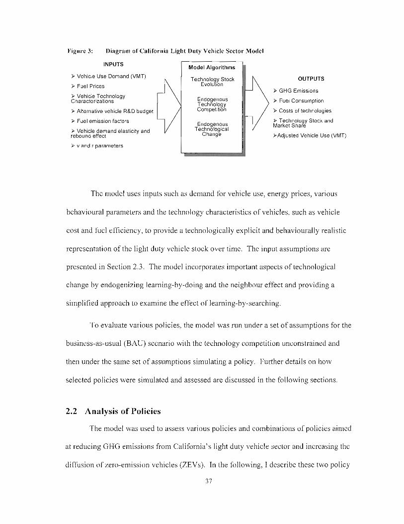
Figure 3: Diagram of California Light Duty Vehicle Sector Model

INPUTS Model Algorithms

9 Vehicle Use Demand (VMT) I P Fuel Prices

9 Vehicle Technology Characterizations

3 Alternative vehicle R&D budget I A 9 Fuel emission factors 'I/ I 9 Vehicle demand elasticity and rebound effect " I 9 v and r parameters

Technolo y Stock ~volu?ion

Endogenous Technology Competition

Endogenous Technologcal

Change

OUTPUTS

3 GHG Emissions

9 Fuel Consumption

k Costs of technologies

9 Technology Stock and Market Share

&-Adjusted Vehicle Use (VM

The model uses inputs such as demand for vehicle use, energy prices, various

behavioural parameters and the technology characteristics of vehicles, such as vehicle

cost and fuel efficiency, to provide a technologically explicit and behaviourally realistic

representation of the light duty vehicle stock over time. The input assumptions are

presented in Section 2.3. The model incorporates important aspects of technological

change by endogenizing learning-by-doing and the neighbour effect and providing a

simplified approach to examine the effect of learning-by-searching.

To evaluate various policies, the model was run under a set of assumptions for the

business-as-usual (BAU) scenario with the technology competition unconstrained and

then under the same set of assumptions simulating a policy. Further details on how

selected policies were simulated and assessed are discussed in the following sections.

2.2 Analysis of Policies

The model was used to assess various policies and combinations of policies aimed

at reducing GHG emissions from California's light duty vehicle sector and increasing the

diffusion of zero-emission vehicles (ZEVs). In the following, I describe these two policy

3 7

goals, GHG emission reductions and ZEV diffusion, under which the selected policies

were assessed. The cost of policy is a key tool in assessing diverse policy measures.

Therefore, I also describe a range of approaches to reporting the costs of actions

attributable to various policies and present how I have chosen to report cost.

2.2.1 Policy Target

The selected policies were compared in the period from 1990 to 2045 under a

two-fold target:

1 . Deep Emissions Reductions: Reduce emissions to 60% below BAU 1990

levels by 2045.

2. Widespread ZE V diffusion: One-half (50%) of all vehicle stock is ZEV by

2045.

In order to compare the policies, each policy was adjusted until it met the two-

fold target. In holding the target constant across the alternative policies, I can consider

differences in the costs of the policies while the benefits of the policy remain primarily

the same. Because emission reductions are possible without the diffusion of ZEVs, I also

conducted analysis to explore how the emission reduction target defined above may be

met without the adoption of ZEVs. The details of this analysis are presented later in this

paper.

Deep Emission Reductions

Under this goal, I adjusted the policy such that it arrives at th le targeted level of

direct GHG emissions by 2045. Direct GHG emissions represent the "tail-pipe"

emissions of the vehicles. Therefore, to meet the deep emission reduction component of

3 8

the target, the policy's direct emissions in 2045 must be 60% lower than the direct

emissions in the business-as-usual scenario in 1990.

While direct emissions provide a good starting point for assessing a policy's

environmental impact, indirect emissions contribute considerably to total emissions in the

transportation sector. I define indirect emissions as those resulting from upstream fuel-

related activities, for example from the extracting, refining and transportation of crude oil

in the case of conventional gasoline vehicles, or from the generation of electricity used in

powering a battery electric vehicle. Therefore, I also examined the impact of indirect

emissions on the total GHG emission levels of the policies assessed.

Incorporating indirect emissions adds a layer of complexity to the analysis. For

instance, an economy-wide policy that taxes greenhouse gases would induce

technological change in the upstream sectors of electricity generation and potentially in

the oil and gas sectors. Such a tax on greenhouse gas emissions would likely result in

decreasing the indirect emissions intensity of electricity generation. However, because

the model represents partial equilibrium, a policy's effect on the indirect emissions and

energy prices is not endogenous. To capture some of these impacts exogenously, the

indirect emission factors are adjusted in the model over time under the policy scenario.

The indirect emissions under the policy scenario are discussed in further detail in Section

2.3.

Widespread ZEV Diffusion

Under this goal, I ensured that the selected policy meets the desired level of ZEV

market penetration. That is, at least 50% of the 2045 vehicle stock is zero-emission

vehicles. As the 2045 vehicle stock is made up of several vintages of vehicles, zero- 3 9

emission vehicle penetration in previous periods has to be sufficiently high to meet this

goal. Note that this goal is not tied to a specific ZEV technology.

2.2.2 Evaluating the Cost of Policy Measures

The principle criterion by which these diverse policies were evaluated is cost. In

order to calculate the cost of a policy my model was soft-linked to a cost accounting

to01.'~ This cost accounting tool was originally developed to link with CIMS in order to

cost a diverse portfolio of policies and thus is well suited for this study. For a detailed

explanation of the cost-accounting tool, see Peters (2006).

The cost of a policy can be defined and measured in a variety of ways. The cost

accounting tool has the ability to return three measures of cost, the financial, perceived

and expected resource cost of a policy. Financial cost of a technology is estimated as the

sum of its capital costs and the present value of its operating costs over its lifespan,

discounted using a social discount rate. The financial costs of a policy represent the

traditional "bottom-up" cost measure, in which consumers make purchase decisions on

the financial life-cycle costs of a technology alone, all consumers are assumed to have the

same cost of adoption, and technology risks are considered non-existent.

The perceived cost provided by the cost accounting tool is defined as the

conventional "top-down" definition of cost. The perceived costs include the intangible

costs of a technology, a discount rate which takes into account real and perceived risks

associated with the technology, and a heterogeneous consumer base. A cost (financial

and/or non-financial) is incurred whenever a consumer deviates from their initial choice

12 As opposed to physically connecting two models, soft-linking involves generating outputs from one model to use as inputs for another model.

4 0

of technology due to a policy. Similarly, a cost occurs when a consumer deviates from

their initial demand for vehicles and/or vehicle use. Both of these costs make up the

perceived cost of a policy.

The expected resource cost provided by the cost accounting tool attempts to

capture the exposte costs of switching or adopting a new technology due to a policy.

Thus, the expected resource cost includes the financial costs and some portion of

intangible costs, a risk premium and market heterogeneity to the extent that /hese values

are real and not a result of marketfailures (for example consumers having imperfect

information when purchasing a vehicle). Like the perceived cost, expected resource cost

would also include welfare costs associated with changes in demand for vehicle use

associated with a policy.'3

The parameters used by the cost accounting tool to calculate the exposte costs of

technologies must be provided by the user. These parameters include the financial costs

and the portion of intangible costs, discount rate and consumer heterogeneity not

attributable to market failures. As discussed below a number of researchers have begun

to collect these data for the light duty vehicle sector. Using these data, I was able to

provide an estimate of the expected resource cost of alternative policies. Therefore, in

this analysis, I report and compare the expected resource costs of the selected policies.

The expected resource costs of policies provides the exposte cost of consumers

switching or adopting a new technology due to a policy. However, to conclude this

discussion of cost, it should be noted what is not included in this definition of cost. First,

13 Welfare costs represent intangible losses of consumer value associated with abandoning a technology or using it less.

4 1

because this cost definition represents the social costs of a policy, emission charges paid

under a tax policy are excluded. Taxes are a transfer of income from payer to the

government and are therefore assumed to represent a gain elsewhere in society and not a

social cost. Second, administration costs associated with alternative policies are not

included. Third, infrastructure costs related to the rollout of new technologies are not

included. Fourth, I did not include any allocation for benefits from emission reductions

in these calculations. Fifth, any macroeconomic costs, for example any costs associated

with a loss of economic activity from a policy, are not reflected in the costs presented

here.

2.3 Input Assumptions and Application to California

In order for the model to simulate various policies for the vehicle sector in

California a number of input assumptions are required. I present the main assumptions

used in the business as usual scenario and their sources below. There is uncertainty

associated with these parameter assumptions. The incorporation of uncertainty analysis

is discussed in Section 2.5.

2.3.1 Demand Forecast and Vehicle Ownership Characteristics

The demand for vehicle use for years 1990 to 2045, measured in passenger

vehicle miles travelled (VMT), is based on data and forecasts generated by the California

Department of Transportation (2005). The demand for 1990 to 2005 is based on actual

data, while the demand for 2005 to 2045 is based on their projected growth rates.

Data from the California Department of Transportation (2005) were also used to

generate an assumption for the average vehicle miles travelled per year per vehicle and

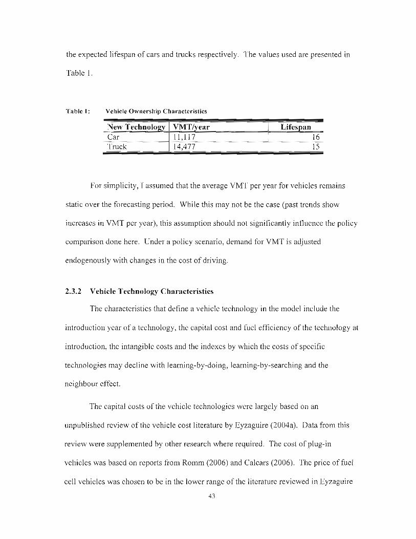
the expected lifespan of cars and trucks respectively. The values used are presented in

Table 1 .

Table 1 : Vehicle Ownership Characteristics

New Technology Car

For simplicity, I assumed that the average VMT per year for vehicles remains

static over the forecasting period. While this may not be the case (past trends show

increases in VMT per year), this assumption should not significantly influence the policy

comparison done here. Under a policy scenario, demand for VMT is adjusted

endogenously with changes in the cost of driving.

Truck 1 14,477

2.3.2 Vehicle Technology Characteristics

The characteristics that define a vehicle technology in the model include the

introduction year of a technology, the capital cost and fuel efficiency of the technology at

introduction, the intangible costs and the indexes by which the costs of specific

technologies may decline with learning-by-doing, learning-by-searching and the

neighbour effect.

VMTIyear 11.117

15

The capital costs of the vehicle technologies were largely based on an

Lifespan 16

unpublished review of the vehicle cost literature by Eyzaguire (2004a). Data from this

review were supplemented by other research where required. The cost of plug-in

vehicles was based on reports from Romm (2006) and Calcars (2006). The price of fuel

cell vehicles was chosen to be in the lower range of the literature reviewed in Eyzaguire

4 3

(2004a) because a relatively conservative introduction year was selected for this vehicle

type. Trucks were assumed to be 25% more expensive than cars of the same technology

type (e.g. gasoline or battery electric) and 30% less fuel efficient relative to the same

cars. Trucks were also assumed to have equivalent declining cost characteristics to the

cars of the same technology type.

The fuel efficiency of vehicle technologies was based on the same review by

Eyzaguire (2004a) and supplemented where needed by fuel efficiency figures provided

by the EPA (2006a). The fuel efficiency of most vehicles was assumed to improve

autonomously at a rate of 0.1% per year. For vehicles that are considered at their early

stages of market diffusion, such as ethanol, hybrid electric, plug-in hybrid and fuel cell

vehicles, the fuel efficiency improvement was assumed to be 0.2% per year.

Several flexible fuel vehicles were included in the model. Ethanol vehicles were

assumed to have a 15/85 split between gasoline consumption and ethanol consumption.

Plug-in electric hybrids were assumed to have a 15/85 split between gasoline and

electricity consumption respectively. Biofuel plug-in electric hybrids were assumed to

have a 15/85 split between ethanol and electricity consumption.

Declining capital costs for technologies were enabled based on the stage of a

technology's development and diffusion. Mature technologies that have reached high

levels of market penetration, like conventional gasoline vehicles, were assumed to be

unaffected by learning-by-doing or learning-by-searching. I assumed that gasoline-

electric hybrids, plug-in hybrids, battery electric and hydrogen fuel cell vehicles could all

benefit from learning. As a technology matures and high levels of market share are

reached, the cost savings resulting from learning was assumed to decline and eventually

44

plateau. Therefore, for those technologies impacted by learning, I specified a cost at

maturity. The cost at maturity was assumed to vary depending on the technology type,

but was set to be a specified level above the lowest cost gasoline vehicle.

There is little empirical evidence for the rate of learning with respect to specific

vehicle technologies. The model-T ford was estimated to have a learning index of 85%

(Abernathy & Wayne, 1974) and the average for manufactured goods is estimated to be

80% (Argotte & Epple, 1990). Electronic devices, which may mimic the curves of many

of the alternative vehicle technologies because of their use of batteries and other

electronic features, have an index from between 72-87% (Dino, 1985). I used subjective

judgment given the range of figures discussed here, and based on the state of the selected

technology's development and diffusion, to establish learning indexes for technology-

specific single-factor learning curves. Note that the learning-by-doing index for a single

factor curve is different from that of a two-factor learning curve because of its more

aggregated formulation.

There is even less evidence for the learning-by-searching index, with the minimal

literature available focusing on the electricity sector (Criqui et al., 2000; Miketa &

Schrattenholzer, 2004; Watanabe, Wakabayashi, & Miyazawa, 2000). I set the values for

selected vehicle technologies to correspond with technologies in the electricity sector that

I deemed as having similar characteristics and diffusion levels. I set the lag between

R&D expenditure and knowledge stock to be five years as per Criqui and colleagues'

(2000) assumption with respect to photovoltaic technology.

A summary of the vehicle characteristics as described above is found in Table 2.

These characteristics are subjected to uncertainty analysis discussed in Section 2.5.

45

Table 2: Summary of Vehicle Characteristics for Cars

Technology Intro. Year

Efficiency Gasoline, High 1 1990 / $12,895 1 1 0.0039

Capital Cost (2000 USD)

Cars Gasoline, Low Efficiency Gasoline, Mid

USD)

0.006 1

Examples of the single-factor and two-factor declining capital cost function for

Cost At

Maturity (2000

--- 1990

1990

Efficiency Diesel Ethanol Gasoline Hybrid Electric Gasoline Plug-in Hybrid Biofuel Plug-in Hybrid Hydrogen Fuel Cell Battery Electric

battery electric cars are shown in Figure 4 and Figure 5. The costs in the single-factor

$23,341

curve decline with increases in experience, expressed as cumulative vehicle stock. In the

F.E. (vmVGJ)

$18,685

1990 1995 2000

2010

201 0

2025

1995

two-factor curve, costs decline with both cumulative experience (in Figure 5 cumulative

0.005 1

production is assumed to be zero) and increases in knowledge stock, driven by

LBD Single- factor

$17,140 $17,174 $23,866

$22,866

---- $22,866

$66,000

$37,776

cumulative R&D investment.

LBD Two- factor

$19,485

$19,485

$19,485

$20,185

$20,685

LBS Two- factor

0.0043 0.0055 0.0028

0.0022

0.0023

0.0037

0.0014

0.95

0.9

0.9

0.75

0.78

-0.17 -0.05

-0.2 -0.07

-0.15

-0.27

-0.25

-0.07

-0. I I

-0.07

Figure 4: Declining Capital Cost (Single Factor Learning Curve) Battery Electric Cars

Cumulative Stock (Vehicles)

Figure 5: Declining Capital Cost (Two factor Learning Curve) Battery Electric Cars

Knowledge Stock($)

A final element defining the vehicle technologies in the model is intangible costs

and dynamics. The values of intangible costs and their dynamics for passenger vehicles

has been the object of various research efforts (Axsen, 2006a; Mau, 2005; Eyzaguire,

47

2004b). For the technologies used in the model, the intangible costs and their dynamics

(i.e. the A and k parameters) were based on empirical research by Axsen (2006a) and an

unpublished report by Axsen (2006b).

As previously discussed, the intangible costs are broken down into two

components, first a fixed component that is not affected by market share of the

technology and second, a dynamic component influenced by market share. This

approach assumes that some elements of certain technologies, for example limited range

or inconvenient fuelling, will always have an intangible cost associated with them

independent of market share and the neighbour effect. Note that a negative number

indicated for intangible cost represents a benefit consumers perceive from that

technology. The intangible characteristics for trucks are similar to those of cars;

however, a premium of -$675O was added to the fixed intangible costs of the trucks to

account for the current preferences of consumers for trucks and SUVs. There remains a

large range of uncertainty surrounding intangible cost characteristics, therefore these

parameters were included in the uncertainty analysis discussed in Section 2.5.

Table 3: Summary of Intangible Vehicle Characteristics for Cars

Technology Fixed Intangible Cost

Variable Intangible Cost

A k

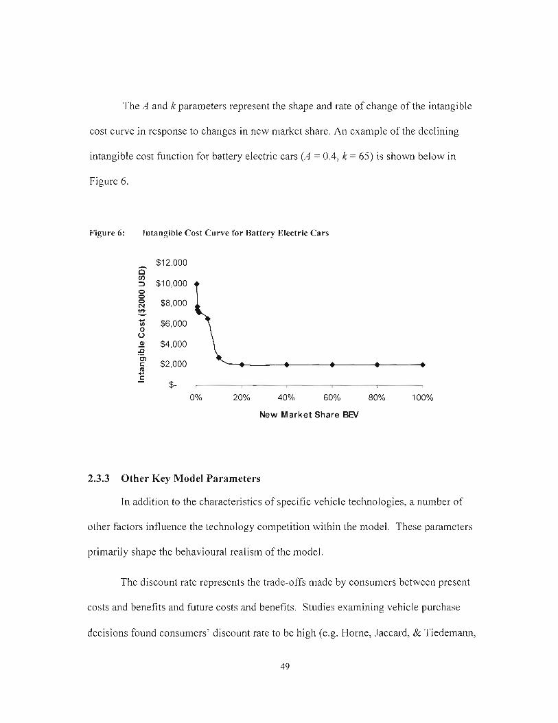
The A and k parameters represent the shape and rate of change of the intangible

cost curve in response to changes in new market share. An example of the declining

intangible cost function for battery electric cars ( A = 0.4, k = 65) is shown below in

Figure 6.

Figure 6: Intangible Cost Curve for Battery Electric Cars

New Market Share BEV

2.3.3 Other Key Model Parameters

In addition to the characteristics of specific vehicle technologies, a number of

other factors influence the technology competition within the model. These parameters

primarily shape the behavioural realism of the model.

The discount rate represents the trade-offs made by consumers between present

costs and benefits and future costs and benefits. Studies examining vehicle purchase

decisions found consumers' discount rate to be high (e.g. Horne, Jaccard, & Tiedemann,

2005). This high discount rate is attributed to a lack of information, limited time to make

decisions, perceptions of risks of new products and the value of waiting for more

information (Dixit & Pindyk, 1994; Hasset & Metcalf, 1994). I chose to use a discount

rate of 25%, which was the value found for California in recent a study (Axsen, 2006a).

This value falls within the range of other studies (Train, 1985; Home et al., 2005).

The so-called variance (v) parameters used in this model enable a more

behaviourally realistic allotment of market share to the various vehicle technologies. A

high v means that the technology with the lowest life-cycle costs captures almost all of

the new equipment stocks, whereas with a low v, equipment market shares would be

distributed more evenly regardless of differences in life-cycle costs. I followed the recent

report compiled by Axsen (2006b) and used a v of 15 for competition within class (i.e.

between cars) and a v of 7 for competition between classes (i.e. between cars and trucks).

As discussed, the overall vehicle demand elasticity and the rebound effect provide

important feedback effects of the model. The vehicle demand elasticity represents the

response of consumers to changes in vehicle price. Once again, there is a range of

vehicle demand elasticities found in the literature (e.g. McCarthy, 1996; Bordley, 1993).

I used a value of 0.5, which is within the range found in the literature. A 1% increase in

the average capital cost of vehicles will result in a 0.5% decrease in the demand for

vehicles and vice versa.

Rebound effect represents the elasticity of the demand for vehicle miles travelled

(VMT) with changes in the cost of driving. The rebound effect characterizes how

increases in efficiency (in this case fuel efficiency) will generally reduce the cost of

driving and thus stimulate some additional use. This phenomenon has considerable

5 0

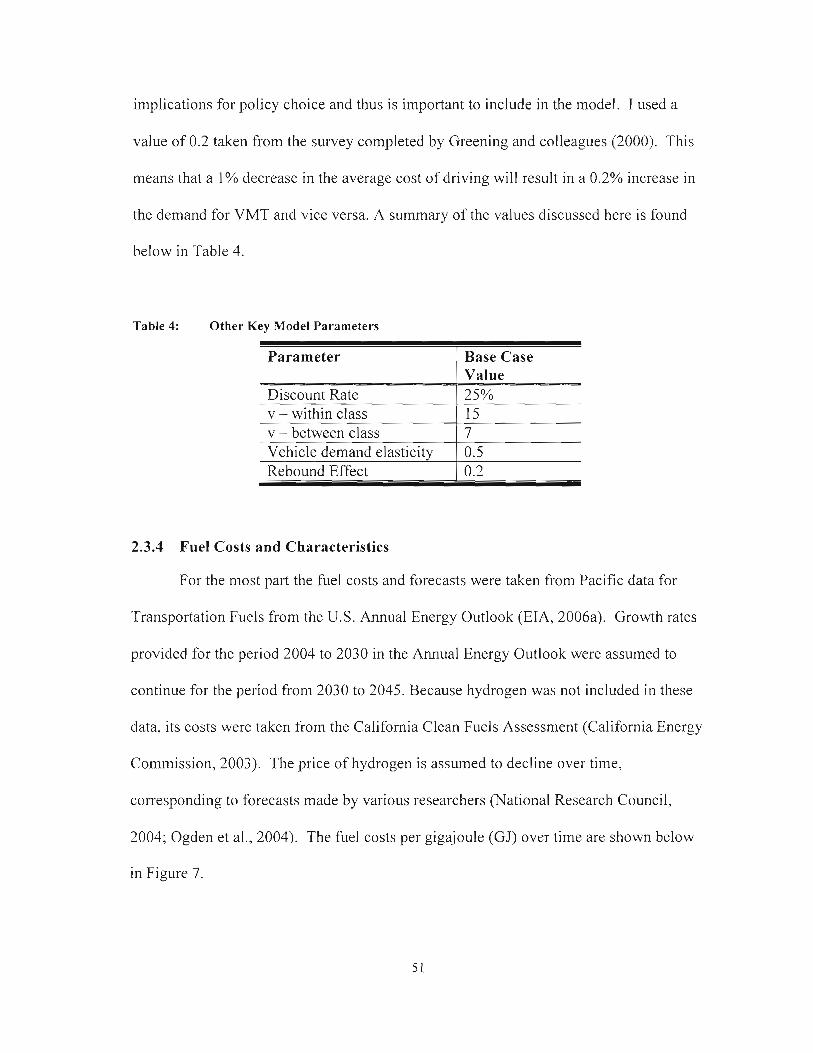
implications for policy choice and thus is important to include in the model. I used a

value of 0.2 taken from the survey completed by Greening and colleagues (2000). This

means that a 1% decrease in the average cost of driving will result in a 0.2% increase in

the demand for VMT and vice versa. A summary of the values discussed here is found

below in Table 4.

Table 4: Other Key Model Parameters - -

Parameter Value

v - within class v - between class

2.3.4 Fuel Costs and Characteristics

For the most part the fuel costs and forecasts were taken from Pacific data for

Transportation Fuels from the U.S. Annual Energy Outlook (EIA, 2006a). Growth rates

provided for the period 2004 to 2030 in the Annual Energy Outlook were assumed to

continue for the period from 2030 to 2045. Because hydrogen was not included in these

data, its costs were taken from the California Clean Fuels Assessment (California Energy

Commission, 2003). The price of hydrogen is assumed to decline over time,

corresponding to forecasts made by various researchers (National Research Council,

2004; Ogden et al., 2004). The fuel costs per gigajoule (GJ) over time are shown below

in Figure 7.

15 7

Vehicle demand elasticity Rebound Effect

0.5 0.2

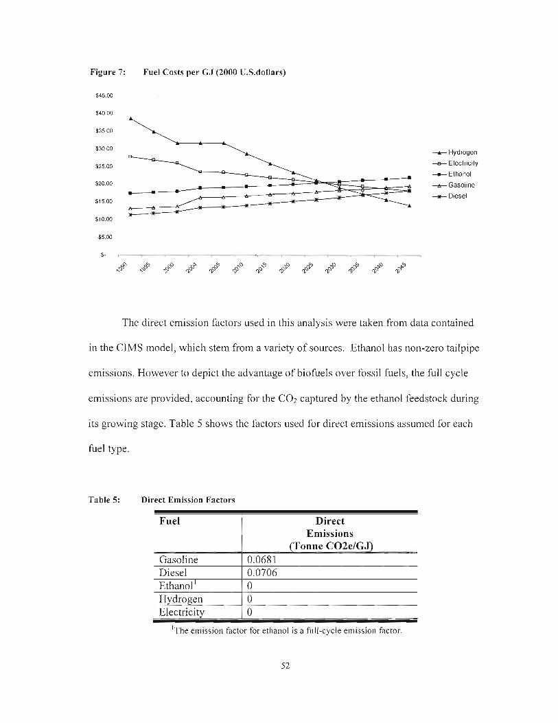
Figure 7: Fuel Costs per CJ (2000 U.S.dollars)

$40.00

$35.00

$30.00 -A- Hydrogen

$25.00 -e- Electricity

-m- Ethanol

$20.00 -A- Gasoline

+Diesel $15.00

$10.00

The direct emission factors used in this analysis were taken from data contained

in the CIMS model, which stem from a variety of sources. Ethanol has non-zero tailpipe

emissions. However to depict the advantage of biofuels over fossil fuels, the full cycle

emissions are provided, accounting for the COz captured by the ethanol feedstock during

its growing stage. Table 5 shows the factors used for direct emissions assumed for each

fuel type.

Table 5: Direct Emission Factors

Fuel Direct Emissions

Gasoline Diesel

Electricity / 0 I The emission factor for ethanol is a full-cycle emission factor.

0.068 1 0.0706

Ethanol ' Hvdro~en

0 0

The indirect emissions for many of the fuels were derived from forecasts made by

Weiss and colleagues (2000). The indirect emissions from California electricity

generation were obtained from Bemis and Allen (2005). The indirect emissions were

assumed to change exogenously over time. I assumed that a moderate economy-wide

policy aimed at reducing greenhouse gas emissions would be in place during the

forecasting period. Therefore, changes in the indirect emissions intensities of various

fuels over time were based on a cap and trade scenario for the U.S. described in EIA

(2006b). However, I assumed that the emissions factors for electricity and hydrogen

decreased more rapidly than the EIA scenario based on California's recently announced

commitment to reduce emissions by 80% by 2050 (Office of Governor, 2006). I assumed

that California's targets would have less impact on the upstream emissions for fuels such

as gasoline and diesel than the electricity sector. Figure 8 shows the indirect emissions

scenario assumed for the forecast period.

Figure 8:

0.12

0.1

0.08

z 1

N

8 0.06 al

c 0 C

0.04

0.02

lndirect Emissions Scenario

--t Hy drogen

-e- Electricity

-m- Ethanol

-A- Gasoline

+Diesel

2.4 Policies Assessed

Section 1.3 in the opening chapter described in general terms the policies selected

for this analysis. Four different policy types were considered. Each policy type was

assumed to have been implemented beginning in 1995. The policies examined were:

a tax on greenhouse gas emissions applied to the direct emissions of

vehicle fuels,

a standard mandating zero-emission vehicle market share requirements,

a purchase subsidy applied to battery electric vehicles (BEVs),

a R&D subsidy targeted at biohel plug-in electric vehicles (BPHEVs).

The purchase subsidy was targeted at BEVs because of its availability in the

1990s as opposed to the other ZEV technologies. The R&D subsidy was targeted at

biofuel plug-in electric vehicles (BPHEVs), a technology currently unavailable, but

which is considered to hold future promise.

Policy combinations were also tested, specifically a purchase subsidy combined

with a tax and a standard combined with a tax. In addition, combining a R&D subsidy

with a tax and a standard respectively was assessed. For these policy combinations, R&D

subsidies were applied from 1990 to 2005 such that the cost of BPHEVs in their first year

available (20 10) was significantly lowered.14

Another part of the policy analysis included the assessment of a delay strategy. In

the delay strategy, no action is taken until 2035 and then either a tax or a standard is put

in place to meet the required target.

Finally, there has been debate on the validity of ZEV diffusion as a policy goal,

particularly with respect to cost-effectiveness (Dixon et al., 2002). Therefore, to explore

how removing ZEV diffusion as a policy goal may affect the results, I also assessed a

ULEV-ZEV standard that allows ultra low-emission vehicles (ULEVs) such as hybrid

electric, plug-in hybrids and ethanol vehicles, in addition to ZEVs, to meet its market

share requirements. This enabled an understanding of some of the trade-offs involved in

attaining a less prescriptive target than the target selected for this study. A summary of

the policy alternatives assessed is provided in Table 6.

14 Battery electric and fuel cell vehicles would also likely benefit from R&D subsidies. However, because of the lack of data to characterize the impact of R&D investment on vehicle costs, testing R&D policies was limited. I targeted BPHEVs to understand how lowering the cost of BPHEV early in the policy run with a R&D subsidy may lower the costs of various policies.

55

Table 6: Summary of Policies Assessed

Tax

ZEV Standard

Purchase Subsidies

R&D Subsidies

ZEV only Standard then Tax

Purchase Subsidies plus Tax

R&D Subsidy plus ZEV Standard

R&D Subsidy plus Tax

Delay then Tax

Delay then ZEV Standard

ULEV-ZEV Standard

Tax applied to direct GHG ernissions of fuels

ZEV new market share mandated

Subsidy is provided to consumer for each BEV purchased.

R&D subsidy is provided for BPHEV research.

ZEV new market share mandated from 1990 to 20 I0 followed by a tax applied to direct GHG emissions of fuels

Purchase subsidy provided for consumers buying BEVs and a tax is applied to direct GHC emissions of fuels

R&D subsidy is provided for BPHEV research and ZEV new market share is mandated R&D subsidy is provided for BPHEV research and a tax is applied to direct GHG emissions of fuels. No policy until 2035 then a tax is applied to direct GHG emissions of hels.

No policy until 2035 then ZEV new market share is mandated

More flexible standard, both ULEVs and ZEVs qualify to meet a market share mandate.

Each policy presented in Table 6 was set such that the target of deep emission

reductions and widespread ZEV diffusion described in Section 2.2 was reached. The

stringency required for each policy to meet this target is detailed in the following chapter.

2.5 Incorporating Uncertainty

Explicit reporting of uncertainty is a key component of a credible and useful

policy analysis (Morgan & Henrion, 1990). This model is a simplified version of reality

that attempts to make predictions over a relatively long period. In particular, predicting

the path of R&D activities and new technology diffusion is fraught with uncertainty.

Section 2.3 describes the input assumptions used in the model's base scenario.

While significant effort was expended to find the most appropriate parameters for this

base scenario, there is inevitable uncertainty around the parameters and input 5 6

assumptions used in this analysis. Therefore, a range of high and low values around the

base scenario assumptions was attributed to the key uncertain parameters. The ranges of

the uncertain parameters were chosen based on subjective judgment in conjunction with

consideration of the ranges provided in literature. I used two approaches for analyzing

the effect of uncertainty on the results, namely, sensitivity analysis and Monte Carlo

analysis.

Sensitivity Analysis

Sensitivity analysis can be used to highlight key areas of considerable uncertainty,

serving two purposes. First, it demonstrates how results may change given changes in

parameters. Second, sensitivity analysis can be used to prioritize uncertainties in the

parameters to inform future research in an effort to narrow the range of results. Single

value sensitivity analysis was performed to understand how single parameter changes

influenced the results. The high and low values of key uncertain parameters are changed

one at a time, the model is then run and the results are recorded. The results are then

presented in a tornado diagram, which helps to evaluate and rank how each uncertain

parameter affects the results. A limitation to this approach is that it does not capture the

effect of multiple uncertainties on the results.

Monte Carlo Analysis

In many cases, using a model with the "best values" for each uncertain parameter

will generate considerably different results than incorporating a more explicit

probabilistic analysis (Morgan & Henrion, 1990). Monte Carlo simulation is a

commonly used technique to capture the effects of uncertainty in large models with a

number of uncertain parameters. Unlike sensitivity analysis, this method may capture the

effects of multiple uncertainties. Monte Carlo simulation was used to estimate a range of

uncertainty in emissions and costs for each policy given a number of uncertain inputs.

I specified a normal probability distribution for each uncertain input. For each

uncertain parameter, the base scenario assumption described in Section 2.3 was selected

as the mean of this distribution and the range of high and low values, described above,

was considered one standard deviation from the mean. The Monte Carlo simulation takes

a random draw from the probability distribution of each uncertain parameter and runs the

model. This was repeated 1000 timesJ5. The distribution of the simulation outputs,

emissions and costs, provides a characterization of the uncertainty of these outputs. The

Monte Carlo simulation was developed using a Visual Basic Macro.

Finally, i t should be noted that other sources of uncertainty in the results exist that

are not fully captured by the sensitivity or Monte Carlo analysis described here. This is

discussed in more detail in Chapter 4.

15 Running the model 1000 times was chosen to balance between model run-time and quality o f results.

5 8

CHAPTER 3: RESULTS AND DISCUSSION

Using the model described in Chapter 2, this chapter presents the results of the

policy analysis. To begin I describe the business-as-usual forecast generated by the

model (Section 3.1). Next, the policy simulations are detailed (Section 3.2). First, I

describe the stringency required for each policy to meet the two-fold target. Second, I

examine the impact of these policies on greenhouse gas emissions and the diffusion of

zero-emission vehicles. Third, I analyze key features of the policies and compare the

costs of policy alternatives. A measure of the uncertainty of the results is provided using

Monte Carlo analysis. Finally, I present sensitivity analysis to understand the

significance of selected uncertain parameters on the results (Section 3.3).

3.1 Business as Usual Forecast

A business as usual (BAU) forecast for greenhouse gas emissions, representing a

scenario in which no additional greenhouse gas (GHG) policy is applied, was generated.

Monte Carlo analysis was used to produce this forecast. The forecast of California's

passenger vehicle emissions, that includes both direct and indirect GHG emissions, was

compared to a similar forecast produced by the California Air Resources Board (CARB,

2004) in Figure 9.

Figure 9: BAU Emissions Forecast (Direct and Indirect Emissions)

300

MODEL .*---i!r-- I - -a- - Nbdel mean +I- 1 standard deviation I

The model's forecast represents the mean of the Monte Carlo analysis and the

error bars depict one standard deviation in each direction from the mean. The standard

deviation around the mean of the forecast increases over time, indicating the increased

uncertainty in predictions of technological change as the forecasting period lengthens.

The forecasts are within 5% of each other and follow a similar increasing trend.

CARB's forecast is slightly higher than my forecast. This variation can be attributed to a

number of possible factors, such as differing assumptions regarding indirect emission

intensities, the policy efforts assumed to be included in the BAU, and assumptions about

the market acceptance of various vehicle types.

The model's BAU forecast for new market share of vehicle technologies is shown

in Figure 10. In the BAU scenario, conventional gasoline vehicles begin to lose market

share over time, as diesel, hybrid electric vehicles, biofuel and plug-in hybrid electric

60

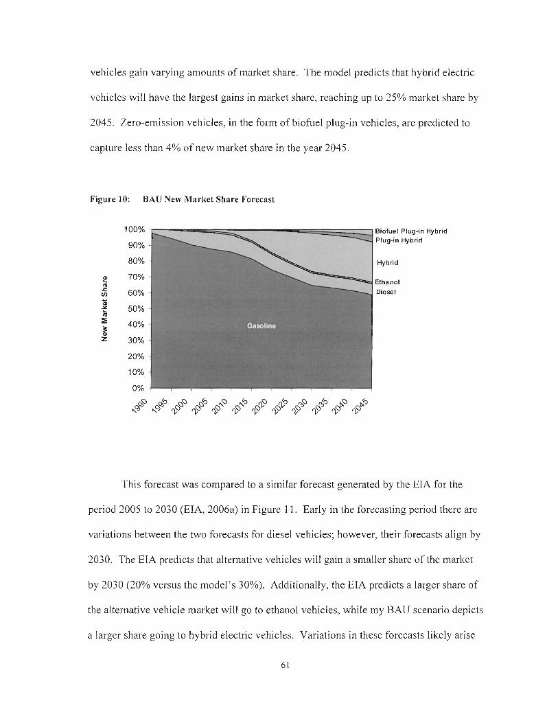
vehicles gain varying amounts of market share. The model predicts that hybrid electric

vehicles will have the largest gains in market share, reaching up to 25% market share by

2045. Zero-emission vehicles, in the form of biofuel plug-in vehicles, are predicted to

capture less than 4% of new market share in the year 2045.

Figure 10: BAU New Market Share Forecast

Biofuel Plug-in Hybrid Plug-in Hybrid

Hybrid

Ethanol Diesel

This forecast was compared to a similar forecast generated by the EIA for the

period 2005 to 2030 (EIA, 2006a) in Figure 11. Early in the forecasting period there are

variations between the two forecasts for diesel vehicles; however, their forecasts align by

2030. The EIA predicts that alternative vehicles will gain a smaller share of the market

by 2030 (20% versus the model's 30%). Additionally, the EIA predicts a larger share of

the alternative vehicle market will go to ethanol vehicles, while my BAU scenario depicts

a larger share going to hybrid electric vehicles. Variations in these forecasts likely arise

from different assumptions regarding the projected costs and market uptake of hybrid and

ethanol vehicles as well as the incorporation of the outcomes of various policy efforts in

the BAU. Uncertainty analysis will in part account for such variations in BAU

assumptions.

Figure I I: EIA Forecast

Hybrid

Ethanol

Diesel

3.2 Results of Policy Comparison

As discussed, the selected policies were set to meet the following two-fold target:

1. Deep Emissions Reductions: Reduce (direct) emissions to 60% below

BAU 1990 levels by 2045.

2. Widespread ZEV dij5usion: One-half (50%) of all vehicle stock is ZEVs

by 2045.

The policies were adjusted using the base scenario parameters to be as stringent

(or as large in the case of incentives) as necessary to meet the target. For simplicity, the

stringency of most of the policies were simply increased (or decreased) linearly over time

as required to meet the target.

3.2.1 Policy Details

The specifics of the policy simulations are detailed in Table 7. The percentage

provided for the ZEV standard is the minimum new market share for zero-emission

vehicles mandated by the policy. For the purchase subsidy, the amount indicated is the

subsidy per battery electric vehicle purchased.

Table 7: Policy Details

ZEV Standard

Purchasc Subsidics

ZEV only Standard then Tan

Purchase Subsidies plus Tax

Delay then Tax

Delay then ZEV Standard

S/ tonne 0 295 310 326 342 360 378 398 418 439 462 485 co, ZEV PA)

2 5 10 15 20 30 50 60 70 80 90

Sk/ BEV 0 15.8 15.5 15.1 14.7 14.3 14.0 13.7 13.3 13.0 12.6 12.3

ZEV 2 5 10 15 25 - f %)

Y tonne - - 425 425 425 425 425 425 C02

In addition to the policies described in Table 7, the use of a research and

development (R&D) subsidy as a policy lever was explored. Combining a R&D subsidy

with a tax or a ZEV standard was also examined. For these policy combinations, R&D

subsidies were applied in the first period (from 1990 to 2005) such that the capital cost of

biofuel plug-in vehicles in their introduction year, 201 0, decreased from $22,866 to

$20,170, which is 80% of their maximum possible reduction in cost. I assumed that

cumulative experience and learning-by-doing is required, in addition to R&D, to reach

the lowest possible cost of a technology.

The stringency of the tax and ZEV standard policies remained the same as

denoted in Table 7. This simplification was chosen because of the lack of empirical

evidence relating to the size and impact of automaker R&D on vehicle capital costs. This

approach allowed for a comparison of the cost-effectiveness of a policy (tax or standard)

with and without the effects of R&D investment, thus providing a crude estimate of the

possible value of R&D investment in meeting the target.

Interestingly, it was found that solely subsidizing R&D (that is not combining the

subsidy with other policies) results in minimal change from the BAU, and does not meet

the target. In the model, R&D investment affects capital costs of a technology but does

not provide any incentive to consumers to adopt the technology. Therefore, few

consumers adopt the new technology and its intangible costs remain high. Since

intangible costs are a significant hurdle for new technologies entering the market, lower

capital costs garnered from R&D investment do not necessarily equate to substantial

gains in market share.

The stringency of the policies should be noted. The tax reaches $485/tonne of

C 0 2 by 2045, translating into an over $4.00/gallon increase in the cost of gasoline. This

equates to an over 150% increase in California's current price of gasoline. The standard

eventually requires 90% ZEV new market share by 2045. Moreover, the subsidy

required for battery electric vehicles is over $10,000 per vehicle, just under one third the

vehicle's capital cost in its first year of availability. As would be expected, the policies

that delay action until 2035 necessitate even higher incentives and more stringent

regulations than those that are applied beginning in 1995.

The stringency of the regulations and size of the market-based incentives required

to meet the target reflect the extent of the challenge in inducing technological change in

the passenger vehicle sector. Stringent policies are necessary even when declining

capital and intangible costs from increases in market share have been endogenized in the

model. However, a number of caveats must be considered when interpreting Table 7.

First, the model does not allow for vehicle technologies that have significantly

decreased in market share to "die out" and become unavailable for the technology

competition. Therefore, the model lacks the ability to depict how a technology could

begin to dominate the market as other technologies become unavailable (Pratt & Hoffer,

1990). More importantly, because R&D investment is not endogenous to the model,

additional innovation and the resulting cost improvements likely motivated by various

policies are not captured. Nevertheless, the caveats described above should have minimal

effect on the comparison of policy alternatives, a key objective of this study.

Next, I present the impact of the policies described above on direct and indirect

emissions and ZEV diffusion.

65

3.2.2 Greenhouse Gas Emissions

Direct GHG Emissions

Direct emissions must reach 40Mt by 2045 in order to be 60% below 1990 levels.

All policies reach this goal in a base scenario, when model parameters are set to their

mean values (Figure 12). Business-as-Usual (BAU) direct emissions reach 201 Mt by

2045,20% lower than the combined indirect and direct emissions considered in Figure 9.

Note that subsidy here refers to a purchase subsidy and not an R&D subsidy.

Figure 12: Direct GHG Emissions for Simulated Policies

- i' 160 w N

140 - VI

6 120 ,- 111 111 .- 2 l oo C)

5 80 'i; .! 60 0

40

20 60% below 1990 Emissions

-2EVStandard

--t Subsidy

+Standard + tax

--c Subsidy + tax

-Delay + standard

-Delay + tax 1

As noted, the stringency of each policy measure was defined using the base

scenario parameters. Subsequently, Monte Carlo simulation was used to analyze how

GHG emissions may be impacted given uncertainty in these parameters (Figure 13).

These data are presented in box-plot form indicating the median, shown with the symbol

+; the interquartile range, which provides a measure of the dispersion of the Monte Carlo

66

results; and the minimum and maximum values resulting from the Monte Carlo runs. In

the box-plot, the interquartile range, represented by the box, depicts the range between

the 25% and the 75% quartile. About half of the data fall within the interquartile range

(hereafter referred to as the "range"). The lines outside the boxes indicate the possible

spread of data up to the data's minimum and maximum values.

Figure 13: 2045 GHG Emissions Levels

1 60% below 1990 Emission levels

Given uncertainty in the model parameters, all of the policies' median 2045

emissions, except the subsidy, hover around the 40 Mt target. The subsidies have a wide

range and their median emissions do not meet the target. These results indicate that the

emission levels resulting from the subsidies are much more sensitive to changes in model

parameters than the other policies. Moreover, while it is possible to reach very low

emissions with subsidies, overall, these policies are less likely to meet stipulated emission

reductions.

Policies incorporating a standard have the narrowest range. Therefore, their

resulting emission levels can be considered the most resilient to change in the uncertain

parameters. This is due to the compulsoriness of standards where tech.nological change is

mandated through regulation. Of the two types of market-based policies assessed, taxes

and subsidies, the taxes have a much narrower range and their resulting emission levels

are thus considered more resilient to uncertainty.

The higher uncertainty of the subsidies can be attributed to their reliance on a

single lever for inducing technological change, that is, consumers' acceptance of a

subsidy towards the purchase of battery electric vehicles (BEVs). If the market

conditions change slightly, for example a change in the predicted cost of BEVs relative to

other vehicles, then consumer acceptance varies widely. All or very few consumers may

be compelled to collect the subsidy and purchase BEVs, resulting in two extremes, either

very low or very high GHG emissions.

The emissions resulting from a tax are less uncertain because of the tax's inherent

flexibility for the decision maker. For example, under a high tax, if the capital cost of an

alternative technology like the BEV is higher than predicted, other competing low-

emission technologies will be adopted in place of the BEV andlor consumers will reduce

their demand for vehicle use.

These results highlight the importance of careful policy design, particularly with

respect to subsidies. For example, creating more options for consumers by broadening

the scope of the subsidy to include all zero-emission technologies would likely reduce its

68

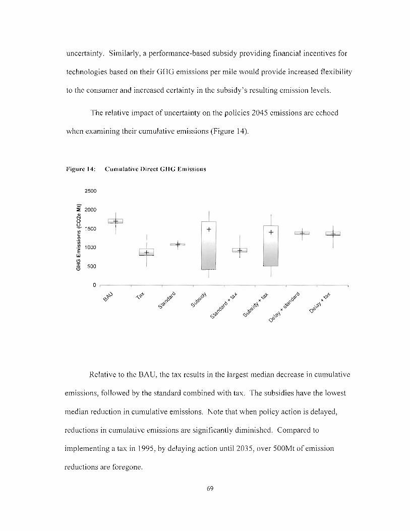
uncertainty. Similarly, a performance-based subsidy providing financial incentives for

technologies based on their GHG emissions per mile would provide increased flexibility

to the consumer and increased certainty in the subsidy's resulting emission levels.

The relative impact of uncertainty on the policies 2045 emissions are echoed

when examining their cumulative emissions (Figure 14).

Figure 14: Cumulative Direct GHG Emissions

Relative to the BAU, the tax results in the largest median decrease in cumulative

emissions, followed by the standard combined with tax. The subsidies have the lowest

median reduction in cumulative emissions. Note that when policy action is delayed,

reductions in cumulative emissions are significantly diminished. Compared to

implementing a tax in 1995, by delaying action until 2035, over 500Mt of emission

reductions are foregone.

Indirect GHG Emissions

The target stipulated reducing direct GHG emissions from the passenger sector.

However, to fully capture the effect of the selected policies on emissions, indirect GHG

emissions must also be considered (Figure 15).

Figure 15:

2,500

- 2,000 s a,

8 2 1,500 U) c 0 .- V) V) 'i 1,000 W C3 I

500

Breakdown of Cumulative GHG Emissions - Direct and Indirect Emissions

'I a lnd~rect

Drect

I Tolal i

(hdirect+Dreclj

Indirect emissions make up 20% of cumulative emissions in BAU and between

25-35% of cumulative emissions of the various policies. Due to the high penetration of

zero-emission vehicles resulting from the policies, when total (indirect and direct)

emissions are considered, the policies' 2045 emissions levels only reach between 19%

and 25% below 1990 levels (rather than 60%). Zero-emission vehicles have zero direct

emissions but do contribute to indirect GHG emissions from the production of alternative

fuels, for example electricity generation.

As discussed in Chapter 2, the indirect emission intensities of the various fuel

types, particularly electricity, were assumed to be decreasing over time. Nonetheless, it

was found that these emission sources play a significant role in overall GHG emissions

for all of the policies. This highlights the importance of considering the upstream

emissions of fuels in policy proposals targeted at reducing emissions from the passenger

vehicle sector.

3.2.3 ZEV Diffusion

The target set out in this study was to reduce GHG emissions while also

increasing the diffusion of zero-emission vehicles (ZEVs) to at least 50% of the total

vehicle stock by 2045. The vehicle stock is made up of several vintages of vehicles,

therefore to meet the goal, ZEVs must be purchased over several periods. The level of

ZEV diffusion varied depending on the policy (Table 8).

Table 8: ZEV Diffusion in Policy Alternatives Tested

2045 New ZEV MS

Share of ZEV in 3% 55% 2045 Stock

79% 77% 62% 78% 75% 55%

Using the base scenario parameters, all policies result in ZEVs contributing to

over 50% of the stock in 2045 (the target level) and at least 60% ZEV new market share

in 2045. The tax is predicted to have the lowest amount of ZEV diffusion. The tax

7 1

results in more diverse means, for example low-emission vehicles and reductions in

vehicle use, being employed to reach the emissions goal. The lower ZEV diffusion

resulting from the tax may be in part attributed to the model's inability to fully capture all

of the aspects of technological change, particularly how one technology may gain

momentum and begin to dominate the market as other technologies "die out". It is highly

uncertain a tax would result in a diverse set of technologies and approaches used to

reduce emissions, as depicted by the model, rather than in a single technology dominating

the market.

Figure 16 shows the Monte Carlo simulation results for 2045 ZEV new market

share for each policy assessed. As expected, by mandating ZEV market share through

regulation, the standard has a high amount of certainty associated with its results. The

market-based policies, particularly the purchase subsidies, have a considerable

uncertainty in their resulting ZEV market share, depicted by their wide range.

Figure 16: 2045 ZEV New Market Share (%)

3.2.4 Key Characteristics of Policy Alternatives

While each policy results in ZEVs making up over 50% of the vehicle stock by

2045, the mix of ZEV technologies that gain share in the market varies by policy. As

expected, the subsidized battery electric vehicle (BEV) dominates the ZEV market share

in the subsidies, whereas the tax induces increases in the market share of the biofuel plug-

in electric vehicle (BPHEV). The ZEV standards result in a split in market share over

time between BEVs and BPHEVs. In the standard, BEVs increase in market share early

in the forecast period, but upon BPHEV introduction, BPHEVs gradually gain and

eventually dominate ZEV market share. These variations in ZEV market share highlight

the potential for policy type, as well as its timing and design, to influence technological

change.

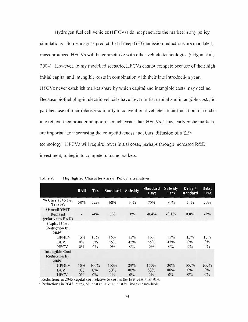
Hydrogen fuel cell vehicles (HFCVs) do not penetrate the market in any policy

simulations. Some analysts predict that if deep GHG emission reductions are mandated,

mass-produced HFCVs will be competitive with other vehicle technologies (Odgen et al,

2004). However, in my modelled scenario, HFCVs cannot compete because of their high

initial capital and intangible costs in combination with their late introduction year.

HFCVs never establish market share by which capital and intangible costs may decline.

Because biohel plug-in electric vehicles have lower initial capital and intangible costs, in

part because of their relative similarity to conventional vehicles, their transition to a niche

market and then broader adoption is much easier than HFCVs. Thus, early niche markets

are important for increasing the competitiveness and, thus, diffusion of a ZEV

technology. HFCVs will require lower initial costs, perhaps through increased R&D

investment, to begin to compete in niche markets.

Table 9: Highlighted Characteristics of Policy Alternatives

% Cars 2045 (vs. Trucks)

50% 72% (58% 70% 75%

Overall VMT Demand -4% I % I % -0.4%

(relative to BAU) Capital Cost Reduction by

2045' BPHEV 15% 15% 15% 15% 15% BEV 0% 0% 45% 45% 45% HFCV 0% 0% 0% 0% 0%

Intangible Cost Reduction by

2045' BPHEV 30% 100% 100% 29% 100% BEV 0% 0% 60% 80% 80% H FCV 0% 0% 0% 0% 0%

' Reductions in 2045 capital cost relative to cost in the fust year available. 2 Reductions in 2045 intangible cost relative to cost in first year available.

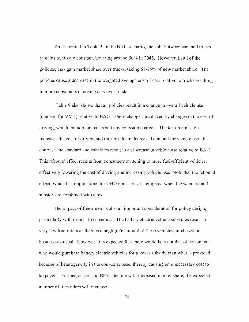
As illustrated in Table 9, in the BAU scenario, the split between cars and trucks

remains relatively constant, hovering around 50% in 2045. However, in all of the

policies, cars gain market share over trucks, taking 68-75% of new market share. The

policies cause a decrease in the weighted average cost of cars relative to trucks resulting

in more consumers choosing cars over trucks.

Table 9 also shows that all policies result in a change in overall vehicle use

(demand for VMT) relative to BAU. These changes are driven by changes in the cost of

driving, which include fuel costs and any emission charges. The tax on emissions

increases the cost of driving and thus results in decreased demand for vehicle use. In

contrast, the standard and subsidies result in an increase in vehicle use relative to BAU.

This rebound effect results from consumers switching to more fuel-efficient vehicles,

effectively lowering the cost of driving and increasing vehicle use. Note that the rebound

effect, which has implications for GHG emissions, is tempered when the standard and

subsidy are combined with a tax.

The impact of free-riders is also an important consideration for policy design,

particularly with respect to subsidies. The battery electric vehicle subsidies result in

very few free-riders as there is a negligible amount of these vehicles purchased in

business-as-usual. However, it is expected that there would be a number of consumers

who would purchase battery electric vehicles for a lower subsidy than what is provided

because of heterogeneity in the consumer base, thereby causing an unnecessary cost to

taxpayers. Further, as costs in BEVs decline with increased market share, the expected

number of free-riders will increase.

75

Finally, the impact of various policies on the capital and intangible cost of ZEVs

is also depicted in Table 9. A policy that results in lower costs for ZEVs early in the

forecasting period will similarly enable a lower cost of ZEV diffusion. In the BAU, the

capital cost of the biofuel plug-in vehicle (BPHEV) reaches its lowest value, a 15%

reduction from its initial cost, by 2045. In contrast, due to increased BPHEV market

share, all policies except the subsidies result in BPHEVs attaining their minimum capital

cost by 2020 (versus 2045 in BAU). The intangible costs of BPHEVs represent an even

larger variation between the BAU and the policy scenarios. In the BAU, BPHEV

intangible costs are reduced from their initial value by 30% by 2045. The tax and the

standard policies result in the intangible costs of BPHEVs reduced by 100% by 2025.

The standard and the subsidies also result in increases in battery electric vehicle

(BEV) market share and thus significant reductions in the capital and intangible costs of

BEVs. Because hydrogen fuel cell vehicles (HFCVs) do not penetrate the market in any

policy simulations, no reductions in their costs are observed. As noted the path of ZEV

costs relative to BAU plays a significant role in the cost of policies, discussed in the

following section.

3.2.5 Costs of Policy Alternatives

This analysis uses expected resource costs to estimate the cost of the policies

relative to BAU. The expected resource cost of a policy is comprised of the cost

associated with consumers switching from technologies that they would have otherwise

adopted in the BAU and the costs associated with shifts in demand for vehicles andlor

vehicle use (VMT). As described in Section 2.2.2, the expected resource cost assumes a

heterogeneous consumer base and includes financial costs, some portion of intangible

76

costs and premium for risk, to the extent that these values are real and not a result of

market failures. Monte Carlo analysis was performed to estimate uncertainty in policy

cost.

First, I compare the cost of policy alternatives implemented in 1990. Next, I

examine how an injection of R&D investment for both the tax and the standard affects

their costs. Finally, I explore the impact of delaying action until 2035 on policy cost.

Policies Implemented in 1990

The costs of policies implemented in 1990 are presented in Figure 17. The costs

are discounted back to 1990 at the rate of 3% per year and presented in year 2000 U.S.

dollars. Discounting costs attempts to capture society's preferences for present versus

future con~urnption. '~ The social discount rate (opportunity cost of capital) was chosen

to fall between the range of 0.5% and 6% per year observed in the literature (IPCC,

1995). The sensitivity of the results to the selected discount rate are explored in Section

3.3. Once again, a box-plot is chosen to present the results. Positive numbers represent a

cost, whereas negative numbers represent benefits derived from the policy. Negative

costs or welfare improvements may occur when the intangible and capital costs of a new

technology decline such that consumers benefit from adopting a vehicle with lower

operating costs (generally fuel costs).

'' Note that the discount rate used here is different from that used in the model to capture how consumers value present and future costs when purchasjng a vehicle.

77

Figure 17: Cost of Policy Alternatives - discounted to 1990 at 3%/year, 2000 U.S dollars

The standard then tax has the lowest median cost, followed by the standard alone

and the combination of a purchase subsidy with a tax. The tax and the subsidy

implemented on their own have the highest median costs. Once again, the purchase

subsidy policies have the widest range of their costs, indicating more uncertainty in their

results.

Because of differences in their cumulative emission reductions, examining the

cost of the policies per tonne of COz reduced, allows a more informative comparison

between the policy alternatives. This so-called cost-effectiveness analysis will remove

the differences in cumulative emission reductions between policies, allowing a

determination of the lowest cost option for meeting the target. Figure 18 shows the cost-

effectiveness or average expected resource cost of the policies per tonne of CO;! reduced.

Note that while costs are discounted in these results, emissions are not.

Figure 18: Cost-Effectiveness of Policy Alternatives per tonne C02 reduced -costs discounted to 1990 a t 3%/year, 2000 U.S dollars

The cost-effectiveness analysis presents a different rank order of the policies than

that based on total costs. The standard and tax combination still has the lowest median

cost per tonne of COz reduced. The tax, standard and the combination of subsidy and tax

are comparable in terms of their median cost-effectiveness."

The combination of subsidy with tax has a much wider range than the tax or the

standard policies. The range of the subsidy-tax combination is $1 05 whereas the range

for the tax is $1 8 and standard is $3 1. The subsidy is the least cost-effective as it has the

17 For a linear marginal abatement curve, we would expect the average costhonne of the tax policy to be half the tax rate applied. For the tax policy, the average cost presented here ($27/tonne) is much lower than the applied tax (tax increases over time to $425/tonne) for several reasons. First, the cost presented here is discounted while the emissions are not (this will lower the average cost/tonne). Second, the tax rate changes over time, however the cost presented here is over the entire forecasting period. Upon adjusting for these factors, it was noted that the average costltonne in a single period was about one third of the tax rate applied in that period. Thus, the shape of the marginal abatement curve for emission reductions in this sector is not linear but likely quadratic.

highest median cost per tonne of C02 reduced. Its costs also have the highest uncertainty.

The relatively poor cost-effectiveness of the subsidy is due to its unpredictable emission

reductions and its reliance on battery electric vehicles, a relatively expensive technology,

to reduce GHG emissions. Note the substantial improvement in the cost-effectiveness of

the subsidy when it is combined with a tax.

The standard and tax policy is most cost-effective as it induces gains in the market

share of ZEVs early in the forecastjng period resulting in reductions in the capital and

intangible costs of ZEV technologies. Then, when the tax is implemented, ZEV market

share continues to grow at relatively low cost to the consumer while other cost-effective

methods of reducing emissions are also introduced, namely the growth in hybrid electric

vehicle market share. Further, the tax neutralizes increases in the demand for vehicle use

caused by the adoption of more fuel-efficient vehicles (rebound effect).

In contrast, while a simple tax results in reductions in the demand for vehicle use

and increases in the penetration of ZEVs, it also relies on a more diversified response and

therefore less early concentration of ZEVs. Thus, the cost savings in the ZEV

technologies are not gained early in the forecasting period. The standard forces

consumers to adopt ZEVs even when more cost-effective reductions could be garnered by

adopting low emission technology or reducing demand. The standard then tax policy

provides the benefits of both the tax and standard by balancing between reducing the

costs of ZEVs for emission reductions in the future and using other cost-effective means

to reduce emissions in the present.

A number of caveats should be highlighted in extrapolating these results from the

modelled environment. First, these simulations assume that both government and the

80

firm are myopic and thus unable to predict and act on the lowest cost path for present and

future emission reductions. That is, both the policy-maker and the firm cannot foresee

the potential reductions in both intangible and capital costs of the various technologies to

be garnered from experience. If one assumes that firms and governments have some

foresight, the results presented here likely overestimate the costs of the policies. This is

particularly relevant for the tax policy as the standard automatically captures many of the

cost savings from experience by forcing the adoption of ZEVs. Second, as previously

discussed, the model does not take into account innovation induced from policy, which

would likely affect the policy costs. In the following section, I present results comparing

the most cost-effective policy discussed above, the standard then tax, with a delay then

act strategy.

Act Early versus Delay Strategy

There remains controversy around the optimal timing of policy to reduce GHG

emissions (Grubb, 1997). To explore how this debate might influence the policy

comparison performed here, I compared the costs of implementing policy in 1990 (with

the cost-effective standard then tax policy) with delaying action until 2035. As discussed

above, a key difference between taking early action and delaying is the large variation in

cumulative emissions between the two strategies. Here I evaluate both the median costs

of the policies (Figure 19) as well as the median cost-effectiveness of the policies (Figure

20). Because of the significance of discount rate in analyzing act now versus delay

strategies, all of these results are shown with varying assumptions of the discount rate.

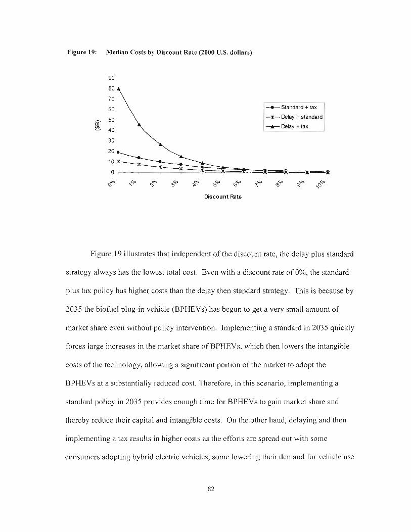
Figure 19: Median Costs by Discount Rate (2000 U.S. dollars)

1 --e standard +tax I I -x- Delay + standard 1

Figure 19 illustrates that independent of the discount rate, the delay plus standard

strategy always has the lowest total cost. Even with a discount rate of 0%, the standard

plus tax policy has higher costs than the delay then standard strategy. This is because by

2035 the biofuel plug-in vehicle (BPHEVs) has begun to get a very small amount of

market share even without policy intervention. Implementing a standard in 2035 quickly

forces large increases in the market share of BPHEVs, which then lowers the intangible

costs of the technology, allowing a significant portion of the market to adopt the

BPHEVs at a substantially reduced cost. Therefore, in this scenario, implementing a

standard policy in 2035 provides enough time for BPHEVs to gain market share and

thereby reduce their capital and intangible costs. On the o.ther hand, delaying and then

implementing a tax results in higher costs as the efforts are spread out with some

consumers adopting hybrid electric vehicles, some lowering their demand for vehicle use

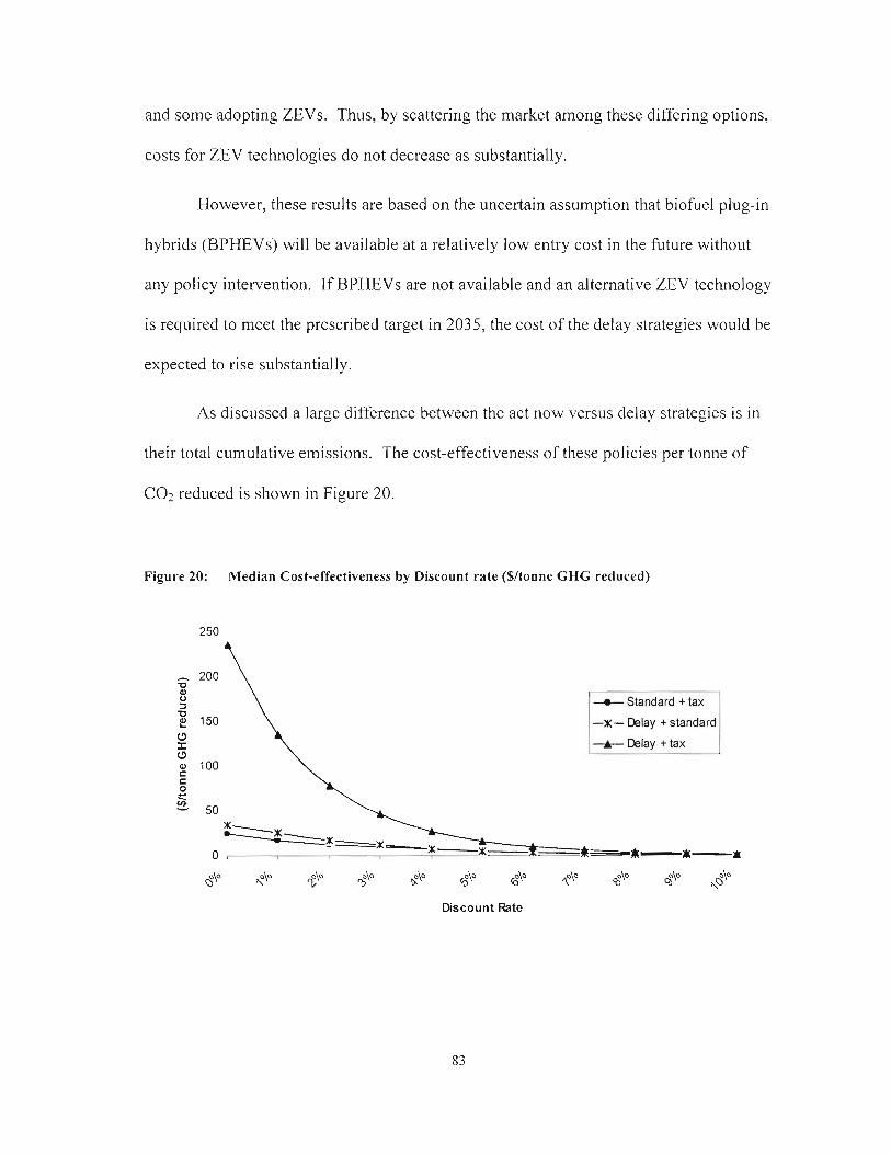
and some adopting ZEVs. Thus, by scattering the market among these differing options,

costs for ZEV technologies do not decrease as substantially.

However, these results are based on the uncertain assumption that biofuel plug-in

hybrids (BPHEVs) will be available at a relatively low entry cost in the future without

any policy intervention. If BPHEVs are not available and an alternative ZEV technology

is required to meet the prescribed target in 2035, the cost of the delay strategies would be

expected to rise substantially.

As discussed a large difference between the act now versus delay strategies is in

their total cumulative emissions. The cost-effectiveness of these policies per tonne of

CO;! reduced is shown in Figure 20.

Figure 20: Median Cost-effectiveness by Discount rate ($/toone GHG reduced)

/ L Standard + tax I I 1 -x- Delay + standard I

I -A- Delay + tax i-

Based on their median results, for a discount rate from 0-6%, the standard then tax

is the most cost-effective policy, followed by the delay plus standard strategy. This is

because the cost of the standard then tax is divided over its large cumulative emission

reductions. However, if the discount rate is increased to 7%, the delay plus standard

strategy becomes the most cost-effective policy. This illustrates the power of

discounting, particularly when examining act now versus delay strategies.

Therefore, if decision-makers can foresee that the cost of BPHEVs will decline

without a policy and they can forego the cumulative emission reductions lost by deferring

action, delaying may be the lowest-cost strategy. However, there is risk involved as the

technological pathway of BPHEVs is uncertain, meaning that delay could involve

significant costs. In a future study, one could account for such risks by determining the

probabilities associated with the technological pathway of ZEVs, such as their costs and

their availability. Using probabilities to establish the expected costs of policies, the risks

of these approaches could be compared.

Potential Impact of R&D Investment on Policy Cost

The potential impact of R&D investment on the discounted costs of select policies

is depicted in Figure 2 1. For these simulations, it is assumed that the R&D subsidy is

targeted at the biofuel plug-in vehicle (BPHEVs) technology from 1990 to 2005. This

R&D subsidy results in a substantial reduction in the capital cost of BPHEVs. The cost

of the policy with and without this R&D investment is compared. Note that the R&D

investment is not included in the cost of the R&D policies shown here.

Figure 21: Impact of R&D Investment on Discounted Costs of Policy - discounted at 3%

As expected the R&D subsidy results in lowering the median cost of both the tax

and the standard policy. It is interesting to note that the R&D investment has a

substantially larger impact on reducing the costs of the tax policy. The standard policy

already has lower BPHEV costs gained through experience without the R&D investment.

In essence, what this exercise is telling us is that if the discounted R&D subsidy is

less than the cost difference between the policy with and without the R&D investment, it

is cost-effective to invest in R&D. Therefore, for the standard, the discounted R&D

subsidy would have to be less than $2B. For the tax, a greater R&D subsidy, up to $10B,

is warranted. Comparing these findings relative to previous government R&D subsidies

targeted at clean vehicle technology shows that over a long period it is not unrealistic to

assume that R&D subsidies could amount to $2B. For instance, the R&D budget for

Partnership for a New Generation of Vehcles (PNGV), a consortium made up of U.S.

government agencies and automakers dedicated to alternative vehicle research, was

$950M in the period from 1997-2000 (Burke, Kurani, & Kenney, 2000). However, a

state acting alone would likely have more limited resources.

It may also be useful to interpret these results through the lens of a firm whereby

they would invest in R&D if it were profitable under a policy scenario. For example, if

firms are required to subsidize BPHEVS so that consumers purchase the vehicles under a

ZEV standard, firms may choose to invest in R&D to lower the cost of BPHEVs and

increase their profit. Alternatively, if firms under the tax policy observe that reducing the

cost of BPHEVS will increase their sales and their profit, they will be motivated to invest

in R&D. Both of these figures presented above are within the realms of the R&D

budgets of the big five automakers. For instance, Ford and Toyota spent just over $7B

and $6B on R&D in 2004 respectively (Technology Review, 2005). Additionally, GM is

reported to have spent $1 B on the development of an electric car (Shnayerson, 1996).

Note that this is a very rudimentary treatment of R&D investment and is meant

only to begin the process of exploring how R&D investment may affect policy cost.

First, there is significant uncertainty around predicting the success and effect of R&D

investment. Second as discussed, this treatment does not incorporate endogenous R&D

induced by policy or the effect of spillover.

3.2.6 Are ZEVs Required?

To understand the emission and costs trade-offs involved in prescribing ZEV

diffusion as part of the target, two additional scenarios were examined. First, I examined

whether the GHG target could be met without the adoption of ZEVs. I calculated the

GHG emissions of a stock entirely comprised of ultra-low emission vehicles (ULEVs),

specifically hybrid electric, plug-in hybrids and ethanol vehicles, all of which have lower

initial capital and intangible costs than ZEVs. It was found that a vehicle stock of 100%

ULEVs would result in significant reductions in GHG emissions over time, but unlike

ZEVs, ULEVs eventually plateau in their capability to reduce GHG emissions. Thus, a

vehicle stock comprised of ULEVs does not result in emissions reaching 60% below

1990 levels by 2045. A stock comprised of 100% ULEVs has 2045 median GHG

emissions almost 60 Mt higher than the 40 Mt target.

Unless vehicle usage is significantly constrained, the diffusion of ZEVs are

required for deep GHG reductions. The next scenario explores the cost and emission

trade-offs if the goal of ZEV diffusion is removed. To this end, a standard policy with

the same market share requirements as the ZEV standard detailed in Section 3.2.1 was

simulated. However, in this more flexible policy, ULEVs, in addition to ZEVs, are

allowed to qualify in meeting the mandated market share (ULEV-ZEV standard).

Table 10 compares the median results of this ULEV-ZEV standard with both the

ZEV only standard and those of the most cost-effective ZEV policy, the standard then

tax.

Table 10: ULEV-ZEV Standard Compared with ZEV Standard and Standard plus tax

Cumulative CHG Emission Reductions ??A / ; l o 771

(C0,e Mt) L L U U 1 0 1 1 2

2045 GHG Emissions (COze Mt) 155 4 0 42

Average Costftonne reduced ($)I 20 29 9

' Costs discounted at 3%/year to 1990 in year 2000 U.S. dollars.

As expected, the ULEV-ZEV standard results in much more moderate emission

reductions then the other policies. However, the ULEV-ZEV standard has a lower

average costltonne than the ZEV standard. Thus, by allowing ULEVs to meet the market

share requirements of the standard, it improves the standard's cost-effectiveness.

However, even with this increased flexibility, the ULEV-ZEV standard remains less cost-

effective than the ZEV standard plus tax policy. The significant emission reductions of

the standard and tax policy over the forecasting period, as well as its ability to capitalize

on the dynamics of technological change, contribute to its cost-effectiveness.

ULEV technology has lower initial costs, less infrastructure requirements and

more certainty about future costs and performance. Thus, depending on the policy

design, if more moderate emission reductions are required, adding an objective of ZEV

diffusion may increase costs. Combining a ULEV policy with a policy that reduces

demand for vehicle use or reduces the GHG intensity of fuels would have even more

impact on emissions (but also on costs). However, for very deep reductions in GHG

emissions from the passenger vehicle sector, ULEV technology is unlikely to be

sufficient and a transition to ZEVs is likely required.

3.3 Single Parameter Sensitivity Analysis

3.3.1 Sensitivity of Cost Comparisons to Social Discount Rate

As noted, there is a considerable range in the discount rates used in policy

analysis. While the social discount rate has particular implications in the debate

surrounding whether we should act now or delay action, it also may affect the results of

the other policy comparisons. A sensitivity analysis was completed to understand the

effect of the discount rate on median policy costs (Figure 22) and cost-effectiveness

(Figure 23).

The rank order of policies in terms of cost and cost-effectiveness is only

marginally sensitive to discount rate. The standard and tax combination has the lowest

total cost over a social discount rate of 0% to 8%. With a discount rate of 9% and lo%,

the subsidy policies become slightly less expensive than the standard plus tax. The

subsidies' costs are generally consistent over time, whereas the standard plus tax's costs

decline over time. Since a higher discount rate emphasizes near-term costs, it favours the

subsidies. The costs of the standard and the subsidy are most sensitive to discount rate

illustrated by the steepness of their curves in both figures. Both of these policies are

predicted to have higher median costs out in time making their results more sensitive to

the chosen discount rate. The standard then tax is the most cost-effective policy over all

tested values of the discount rate.

Figure 22: Sensitivity of Median Policy Costs to Social Discount Rate

&Tax

-x- Standard

+Subsidy

--e Standard+tax i+ SUbsidy+tA

Figure 23: Sensitivity of Median Cost-effectiveness to Social Discount Rate

I 1 4- Tax I -x- Standard

+Subsidy

-o- Standard+tax

i--

Discount Rate

3.3.2 Determining Key Uncertain Parameters

While Monte Carlo simulation provides an aggregated depiction of the influence

of uncertainty on the results, it cannot be used to differentiate between the effects of one

uncertain parameter over another. In this section, I perform single parameter sensitivity

analysis, quantifying the fluctuation of selected results by a change in a single parameter

in the model. This analysis allows for a better understanding of where key uncertainties

lie and may help to inform future research and modelling endeavours, for example by

prioritizing efforts in narrowing the uncertainty of certain parameter values.

The following results are broken up into two parts. First, I examine the sensitivity

of the 2045 GHG emission levels of the selected policies (Figure 24). Second, I explore

the sensitivity of 2045 ZEV new market share (Figure 25). For this analysis, the high and

low values of key uncertain parameters were changed one at a time. For each scenario,

the results from the five parameters that contribute to the most fluctuation from the base

scenario are presented, from highest deviation from the base scenario to lowest deviation,

in a tornado diagram.

The bars of the tornado diagram represent the change in output with a change in

the corresponding parameter. The value of the changed parameter is written beside the

bar. For example, Figure 24 - BAU, analyzes the sensitivity of BAU 2045 emission

levels to changes in uncertain parameters. The BAU base parameter emissions are 201

Mt, represented by the vertical line in the diagram. The discount rate shown here

represents the value used in the model to capture vehicle purchase decision-making, not

the social discount rate discussed in the previous section. Decreasing the discount rate,

from its base value, 25%, to 20% reduces the emissions to 179 Mt; similarly increasing

the discount rate to 30% increases the emissions to 21 1 Mt. The BAU emissions are

most sensitive to the variance parameter characterizing the heterogeneity of consumers

within a class of vehicles (within class v). Decreasing v to 11, malting consumers more

sensitive to life-cycle costs of technologies, decreases emissions to 173 Mt. On the other

hand, decreasing consumers' sensitivity to life-cycle costs by increasing v to 19,

increases emissions to 2 13 Mt.

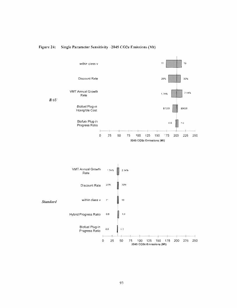
Figure 24: Single Parameter Sensitivity -2045 C02e Emissions (Mt)

within class v

Discount Rate

VMT Annual Growth Rate

BAU

Biofuel Plug-~n Intangible Cost

Biofuel Plug-in Progress Ratio

*-++I 1 -: 0 25 50 75 100 125 150 175 200 225 250

2045 COZe Emissions (Mt)

VMT Annual Growth 1.74% 14%

Rate 0 Discount Rate 20" 1 30%

within class v

Hybrid Progress Ratio 0.8 1 1.0

Biofuel Plug-in Progress Ratio

0 8 1 1.0

0 25 50 75 100 125 150 175 200 225 250 2045 C02e Emissions (Mt)

Figure 24 continued.

Biofuel Plug-in Progress Ratio

0.8 b 7.0

within class v r + l 19

Discount Rate 20% dl 30%

I VMT Annual Growth I 2.14%

Rate

+ ' 1 I !-I 1 -4

0 25 50 75 100 125 150 175 200 225 250

2045 C02e Emissions (Mt)

$29.779

Battery Electrc Vehicle Capital Cost

Battery Electric - - - Vehicle ProgressO.78 o 98

Ratio Suhsidv I

$45.779

- within class v 11

$7000 1 $9000

Battery Electric Intangible Cost

19

Discount Rate 2 0 1

- - - -. ~- 30%

I

I-T- I . - ,--- -t+.-'

0 25 50 75 100 125 150 175 200 225 250

2045 C02e Emissions (Mt)

As in the case of the Monte Carlo analysis, the purchase subsidy emissions are

most sensitive to changes in uncertain parameters. For example, a shift in the starting

capital cost of battery electric vehicle from the base value of $37,779 to $29,779

decreases 2045 emissions from 39 Mt to only 1 Mt. A similar increase in the capital cost

results in an increase in emissions to 20 1 Mt. The subsidy is also very sensitive to the v

parameter and the discount rate. As expected, the subsidy is highly sensitive to the

parameters characterizing the battery electric vehicle (BEV) technology, such as capital

and intangible costs and the progress ratio, which dictates how quickly costs of electric

vehicles will decline with experience.

The standard is the least sensitive to uncertainty because of its compulsory nature.

Therefore, its emissions change only very slightly with changes in the parameter values.

The BAU and policy runs are sensitive to a number of common parameters. The BAU,

the tax and the standard results are all sensitive to the discount rate, the within class v

parameter and the annual growth rate for vehicle use (VMT). While the subsidy is most

sensitive to changes in the characteristics of battery electric vehicles, the BAU, standard

and tax are more affected by changes in the parameters of the biofuel plug-in and the

hybrid electric vehicles.

Figure 25 shows the sensitivity of 2045 ZEV new market share to changes in the

parameters.'s For the most part these results echo those found in Figure 24. Once again,

the subsidy is the most sensitive to uncertain parameters. Again, both the BAU and the

policies are sensitive to the within class v parameter and the discount rate. The ZEV

diffusion of the tax is sensitive to the plug-in vehicle progress ratio. For the market-

'' The standard was not included in Figure 25 as it mandates ZEV market share. Thus, changes in uncertain parameters will not affect the standard's 2045 ZEV new market share.

9 5

based policies, ZEV penetration is sensitive to the relative costs of other competing

technologies.

Figure 25: Single Parameter Sensitivity -Selected Policies 2045 ZEV New Market Share

19

within class v

$7000

Biofuel Plug-in IT^'^^^^ Intangible Cost 1 1 (

20% h 30%

Discount Rate

Hybrid Progress Ratio 0'8n1 O

Biofuel Plug-in Progress Ratio

F- -- I i i

0 Oh 20% 40% 60% 80% 100%

ZEV 2045 Market Penetration

Figure 25 continued.

Biofuel Plug-in 1 0 Progress Ratio

within class v 11

Plug-in Progress Ratio

Discount Rate

Hybrid Progress Ratio 0.8 0 1.0

1 L I I

0% 20% 40% 60% 80% 100%

2045 ZEV Market Penetration

$29,776

Battery Electric Capital Cost I 1 1

.

within class v "1

Battery Electric $7000 $9000

Intangible Cost

Battery Electric - Progress Ratio

Discount Rate 30%

b t - ' + 0% 20% 40% 60% 80% 100%

2045 ZEV New Market Share

0.98

To summarize, results presented here are most sensitive to changes in the following:

the variance parameter, which characterizes the heterogeneity of

consumers purchasing within a vehicle class, such as cars,

the discount rate used to characterize vehicle purchase decisions,

the forecast for vehicle use,

zero-emission vehicle characteristics, specifically their capital and

intangible costs and the rate in which costs decline with increases in

market share and experience,

ultra-low-emission vehicle specifications, such as hybrid electric vehicles

and plug-in electric vehicles.

CHAPTER 4: SUMMARY AND CONCLUSIONS

4.1 Summary

The objective of this research was to assess various policies for increasing the

market penetration of zero-emission vehicles and reducing greenhouse gas emissions in

the passenger vehicle sector. Policies evaluated included a tax on GHG emissions, a

standard mandating ZEV market shares and a purchase subsidy for battery electric

vehicles. Combinations of these policies were examined, as was the potential for

research and development investment to lower the cost of meeting these objectives.

In order to assess the policies, I built a model of the passenger vehicle sector and

applied it to California. It incorporated both widely accepted dynamics of technological

change, such as learning-by-doing, as well as more novel concepts, such as a declining

intangible cost function to capture the neighbour effect and a two-factor learning curve to

explore R&D effects. The model was used in tandem with a cost-accounting too! in order

to estimate the expected resource costs of selected policies. Monte Carlo simulation was

used to assess how policies may be affected by uncertainty.

Policy alternatives were assessed in meeting a two-fold target of reducing GHG

emissions from the passenger vehicle sector to 60% below 1990 levels in 2045 while

increasing ZEV diffusion to at least 50% of vehicle stock by 2045. For each policy, I

reported the direct and indirect GHG emissions, the ZEV diffusion and the cost of the

policy. In addition, the impact of uncertainty on each of these factors was presented.

The policies differed in their cumulative GHG emission reductions. The tax

resulted in the largest cumulative reduction in emissions. The tax not only induced

technological change but also had the largest impact on consumer demand for vehicle

use, lowering overall demand for vehicle-miles-travelled (VMT) by 4%. The standard

and purchase subsidy both resulted in a 1% increase in the total demand for VMT, a

rebound effect resulting from the lowered cost of driving induced by these policies.

Indirect emissions from upstream fuel production were found to be an important

contributor to overall emissions in both the BAU and policy simulations. Indirect

emissions were estimated to make up 20% of total GHG emissions in BAU, and from 25-

35% of total GHG emissions of various policy alternatives. When indirect emissions

were included, the 2045 GHG emissions were found to reach only 19-25% below 1990

levels, rather than the target of 60% below 1990 levels.

The standard then tax policy, which consisted of a relatively conservative

standard (reaching 25% ZEV market share in the period from 1990 to 201 5) followed by

a strong tax ($425/tonne of C02) for the remainder of the forecasting period, had the

lowest median total cost and was found to be the most cost-effective policy per tonne of

C02 reduced.lg The standard then tax policy had a median average expected resource

cost of $9/tonne COz reduced, three times less than the second most cost-effective policy,

the tax alone, at $27/tonne COz. Three of the policies tested were comparable in terms of

cost-effectiveness, the standard, the purchase subsidy combined with tax and the tax

alone. The purchase subsidy was estimated to be the least cost-effective policy, having

19 Unless otherwise noted, all policy cost information refers to a case when costs are discounted at 3%/year back to 1990.

100

the highest median costhonne reduced at $1 601 tonne C02. The standard then tax policy

was the most cost-effective alternative over discount rates of zero to ten percent.

The standard then tax policy was found to be the most cost-effective policy for

two reasons. First, this policy forces market concentration in ZEV technology early in

the forecasting period, resulting in declining ZEV capital and intangible costs. Second,

by implementing a tax when the standard is removed, a signal is sent for consumers to

lower their demand for vehicle use tempering any rebound effect from the increased fuel-

efficiency of the vehicle fleet. Additionally, the tax portion of this policy also increases

cost-effectiveness as it allows more flexibility in how consumers respond (for instance

purchasing a hybrid electric vehicle rather than a ZEV). A standard or a tax,

implemented on its own, provides a portion of these benefits but not all of them, resulting

in higher costs relative to the combination of a standard then tax.

Given a successful R&D program targeted at reducing the capital cost of biofuel

plug-in hybrids (BPHEVs), R&D investment could lower the cost of a policy. R&D

investment was estimated to lower the expected resource cost of the tax and the standard

policies by approximately $1 OB and $2B respectively. These findings can be interpreted

as an estimate of the maximum expected resource cost savings to be gained from

successful R&D investment in meeting the prescribed target. In the context of this study

and its assumptions, the benefits of R&D investment over $10B and $2B for a tax and

standard do not outweigh the resulting savings in their expected resource costs. However,

the depiction of R&D in this analysis is rudimentary and further work in this area is

required.

Further, it was observed that the prescribed target could be met even if policy

action was delayed until 2035. However, by delaying, over 500 Mt of cumulative

emission reductions would be lost. Implementing a standard then tax policy in 1990 was

found to be more cost-effective than delaying action until 2035 for a discount rate of less

than 6%. Because of the long forecasting period, the results of this comparison are

particularly sensitive to the assumptions regarding the discount rate.

It was observed that in order to meet the target, the policy alternatives had to be

relatively stringent. The size of the tax, subsidy or market share mandate of the policies

suggests that the challenges involved in transitioning the passenger vehicle sector to zero-

emission technology are substantial. Finally, the diffusion of ZEV technology was found

to be required to reduce 2045 emissions to 60% below 1990 levels. Ultra-low-emission

vehicles, while providing moderate reductions will not result in this level of deep

emission reductions. In the near term, ULEVs have lower life-cycle costs than ZEVs.

Therefore, there may be a trade-off between attaining cost-effective GHG emissions

reductions in the present versus transitioning the vehicle stock to zero-emission

technology to achieve deep emission reductions in the future.

Uncertainty analysis was reported for all of the major findings. While all of the

predictions made for the selected policies are subject to uncertainty, the results estimated

for the purchase subsidies are particularly uncertain. The parameters that have the most

influence on the results are assumptions regarding the heterogeneity of consumers

purchasing within a specific class of vehicles, the discount rate characterizing vehicle

purchase decisions, the forecast for vehicle use and the costs of zero-emission and ultra

low-emission vehicles.

4.2 Model Limitations and Areas for Future Research

This study used a model of the passenger vehicle sector to assess a variety of

policy alternatives in inducing ZEV diffusion and reducing GHG emissions in the sector.

While this model provides a satisfactory representation of the vehicle sector and of

technological change, it also has a number of limitations. In particular, I identify four

caveats in extrapolating the results from the modelled environment. These limitations in

the model may provide good areas for future research. Areas in which this analysis could

be further extended are: (1) full-equilibrium analysis (2) firm-level representation (3)

evaluation of other policy measures (4) treatment of technological change.

4.2.1 Full-Equilibrium Analysis

The model used in this analysis represents a partial equilibrium system. While

demand changes due to shifts in the price of vehicles and the cost of driving were

endogenous in the model, the cost of fuels and the indirect emissions intensity of fuel

types were exogenous. Further, macro-economic effects such as changes in GDP or

income due to a policy are not included in the model's cost results.

Therefore, changes in the cost of fuel from variations in fuel demand due to

policies were excluded from this analysis. In general, the policies assessed resulted in a

decrease in the demand for gasoline while the demand for electricity and/or biofuel

increased significantly. Such changes in the demand for fuels would likely influence the

costs of these fuels thereby altering the results. Enabling a full-equilibrium analysis

would account for any of these supply-side effects.

Further, a full equilibrium analysis would enable a more thorough depiction of

how shifts in the indirect emissions intensities of various fuels may be influenced through

policy. This would allow a more accurate assessment of policies targeted at both indirect

and direct vehicle emissions, such as an economy-wide tax on greenhouse gas emissions

or a low-carbon fuel standard. Finally, a model that moves towards full-equilibrium

would enable more complete cost results by capturing any macro-economic effects of the

policies such as changes in economic activity, government revenues and employment.

The model used in this study is based on CIMS-T, a component of the economy-wide

model CIMS. Building a California CIMS, and incorporating the model, would enable

modelling efforts to move toward full equilibrium.

4.2.2 Firm-level representation

The decision-agent in the model is the consumer. When there is demand for new

vehicles, the market share of vehicle technologies is determined by an algorithm based on

the life-cycle costs, discount rate and heterogeneity of vehicle consumers. This approach

operates under the assumption that vehicle technologies appear to supply consumer

demand. How firms (in this case automakers) supply this demand is represented in the

model in two ways.

First, when market share in a technology increases, the costs of a new technology

may decline with learning-by-doing in part as the firm gains experience with the

technology. Likewise, an influx of R&D investment may reduce a technology's capital

costs through firm-level research. This provides a representation of many elements that

influence vehicle stock turnover and technological change. However, there are a number

of potentially significant factors regarding the firm that are not incorporated in this

lo4

analysis. Therefore, the model is unable to fully capture how firms may affect (or be

influenced to affect) technological change.

First, the analysis does not incorporate how policies may drive innovation through

greater R&D investment and how spillovers may influence the firms' R&D decisions.

Second, this analysis assumes that firms have no foresight with respect to future policies

and the outcomes of R&D and experience. Varying assumptions regarding firm foresight

would affect the policy results. Third, this study does not analyze the concept of cross-

subsidization, where a firm may subsidize the sale of clean vehicle technologies using

profits from other vehicle sales in order to meet a regulation or influence the market.

While this may be implicit in the model when simulating a standard, quantifying cross-

subsidization would require further research.

Enhancing firm-level representation, whether incorporated into the model used

here or by linking this model with a firm-level model, would enable many of these effects

to be incorporated into the policy assessment. Future studies should seek to endogenize

firm-level decisions in their analysis, particularly with respect to spillover and foresight.

The impact of cross-subsidization and R&D investment on vehicle technology is

not well documented in the literature. A significant hurdle to this research is a lack of

data, which are rarely released by automakers for competitive reasons. Creative methods

will be required to analyze these areas, perhaps forming partnerships with automakers to

exchange information or using estimates to create scenarios for analyzing how these

effects may influence policy.

4.2.3 Further Policy Alternatives to be Assessed

In this analysis, a subset of policy alternatives was selected based on their

relevance in meeting the goal of deep emission reductions and increased ZEV diffusion.

The policy alternatives were then determined using trial and error to meet these goals.

Because of modelling complexity and programming limitations, none of these policies

was optimized for the lowest cost path for the prescribed target. Therefore, a so-called

optimal policy was not determined. Such an optimal policy would provide a good a basis

from which to compare the policy alternatives tested here. Note that an optimal policy is

not exempt from uncertainty; therefore, uncertainty analysis must also be incorporated

into such an evaluation. This could be considered in future studies.

Further, to maintain a reasonable scope, the number of policies assessed were

limited. However, future research efforts could include evaluation of policies that

influence indirect emissions, such as the low carbon fuel standard recently introduced in

California. Additionally, it was found that policies used in combination were proven to

be a cost-effective method of reducing GHG emissions and inducing technological

change. This research could be extended to include additional policy combinations with

varying stringencies to better understand the mechanics of how policies act in

combination. Finally, policies were simulated to begin in 1990 and while it is expected

that the findings can be extended to the present, it warrants performing further analysis to

confirm this assumption. The model developed for this study is capable of simulating

additional policies.

4.2.4 Treatment of Technological Change

While the model attempts to capture a large portion of the dynamics of

technological change, there remain areas in which the representation of technological

change could be further enhanced. For instance, it was observed that relatively stringent

policies were required to induce substantial technological change. The rigidity of the

model to relatively strong policy signals may be attributed to a number of factors that

could be investigated. First, as discussed above, the model does not endogenize

innovation resulting from R&D investment driven by policy. Second, the model does not

allow for technologies that see a sharp decrease in market share due to a policy to become

unavailable for competition. Implementing a so-called "sunset" function, described in

Peters (2006), would likely result in requiring less stringent policies for inducing

technological change.

The results are sensitive to a number of uncertain parameters. The results were

found to be most sensitive to the assumptions regarding consumer heterogeneity, the

discount rate and selected technology characteristics such as capital costs. Because of

their potential impact on policy assessment, these areas warrant further empirical study to

reduce the uncertainty about these values.

Further, while working with the model, I observed that both the BAU and the

policy forecasts were very sensitive to the initial intangible costs selected for the various

vehicle technologies. Research into the intangible costs of vehicle technologies is

relatively limited, and given their importance in the results in hybrid models, I

recommend that empirical research in the non-financial costs of vehicles be continued.

At a minimum, research incorporating vehicle intangible costs must undertake

considerable uncertainty analysis on these parameters.

4.3 Conclusions

Understanding the limits of this model and inherent uncertainties in forecasting

over a fifty-year period, there remain lessons for both the researcher and policy-maker.

In the following, I present a number of conclusions that can be reached from this

analysis.

First, relying solely on technological change to meet a reduction of 60% below

1990 levels by 2045 in the passenger vehicle sector will require a transition to zero-

emission vehicles. This transition will require strict regulations and/or strong market-

based signals.

Second, a policy combination of a standard then a tax cost-effectively leverages

key aspects of technological change such as learning-by-doing and the neighbour effect.

The standard lowers capital and intangible costs of targeted technologies by forcing their

adoption. Once technology costs are lowered, implementing a tax tempers any rebound

effect and allows consumers more flexibility to cost-effectively reduce their emissions.

Such combinations hold promise for minimizing the cost of inducing technological

change towards zero-emission vehicles and reducing GHG emissions.

Third, intangible costs are likely to play a vital role in technological change and

therefore policies should aim to induce both declining capital and intangible costs. For

instance, R&D policies on their own may not affect intangible costs of technologies and

therefore may be more successful when combined with other policies.

Fourth, the impact of indirect GHG emissions will become increasingly

significant with the adoption of ultra low and zero-emission vehicles. Therefore, in

addition to policies aimed at reductions in direct GHG emissions from the passenger

vehicle sector, policies that target indirect emissions should be explored.

Fifth, the cost of deep GHG emission reductions in the passenger vehicle sector

should be compared to the cost of reducing emissions in other sectors in the economy.

To meet economy-wide emission targets, it may be less costly to reduce GHG emissions

from other sectors while seeking more moderate emission reductions from the passenger

vehicle sector. Depending on the policy design, if only moderate GHG emission

reductions are required from the passenger vehicle sector, abandoning zero-emission

technology for ultra-low emission technology may provide more cost-effective GHG

reductions. The emission reductions available from the diffusion of ultra-low emission

technology are limited compared to those available from zero-emission technology.

Sixth, uncertainty analysis has important implications for policy comparison. The

robustness of a policy's expected results varies by policy type. Market-based policies

that are not flexible, such as purchase subsidies targeted at a single technology, are

subject to the most uncertainty.

Finally, future research of a similar nature should consider the following areas:

moving to full-equilibrium analysis

increasing firm-level representation

enhancing the treatment of technological change, particularly

endogenizing R&D.

REFERENCE LIST

Abernathy, W.J., & Wayne, K. (1974). Limits of the learning curve. Harvard Business Review, September - October.

Argotte, L., & Epple, D. (1990). Learning curves in manufacturing, Science, 247,920- 924.

Aufhamrner, M., Hanemann, M., & Szambelan, S. (2006). Transportation in Managing Greenhouse Gas Emissions in CalifOrnia. UC Berkeley: The California Climate Change Center. Retrieved December 12,2006, from http://calclimate. berkelev.edu

Axsen, J. (2006a). Consumer preference dynamics for hybrid electric vehicles: Combining stated and revealed choice models to inform CIMS. Unpublished Master's of Resource and Environmental Management, Simon Fraser University.

Axsen, J. (2006b). Recommendationsfor Transportation Behuvioural Parameters (v, i, r). Simon Fraser University, Burnaby, BC: Energy and Materials Research Group.

Azar, C., & Dowlatabadi, H. (1 999). A review of technical change in assessment of climate policy. Annual Review of Energy and the Environment, 24, 5 13-544.

Azar, C., Lindgren, K., & Andersson, B.A. (2003). Global energy scenarios meeting stringent C 0 2 constraints - cost-effective he1 choices in the transportation sector. Energy Policy, 31, 961 -976.

Barreto, L., & Kypreos, S. (2004). Endogenizing R&D and market experience in the "bottom-up" energy-systems ERIS model. Technovation, 24(8), 61 5-629.

Bemis, G., & Allen, J. (2005). Inventory ofCalifornia greenhouse gas emissions and sinks: 1990 to 2002 update. California Energy Commission Staff Report, California. Retrieved December 12, 2006, from http://www.energy.ca.gov/2005pub1ications/CEC-600-2005-025/CEC-600-2005- 025 .PDF

Bohringer, C. (1998). The synthesis of bottom-up and top-down in energy policy modelling. Energy Economics, 20, 234-248.

Bordley, R. (1 993). Estimating Automotive Elasticities from Segment Elasticities and First ChoiceISecond ChoiceData. The Review of Economics and Statistics, WOn/(3), 401-408.

Boston Consulting Group (1 968). Perspectives on Experience. Boston Consulting Group Inc.

Burke, A.F, Kurani, K.S, & Kenney, E.J. (2000). Study ofthe Secondary Benefits of the ZEV Mandate. Prepared for California Air Resources Board. August 2000.

Calcars. (2006). All About Plug-in Hybrids. Retrieved December 12, 2006, from http://www.calcars.or~vehicles.html

Calef, D., & Goble, R. (2005). The Allure ofirechnology: How France and Cal$ornia Promoted Electric Vehicles to Reduce Urban Air Pollution. Fondazione Eni Enrico Mattei. Retrieved November 14, 2005, from http://ideas.repec.org/p/fem/femwpa/2005.7.html

California Air Resources Board. (2004). Staflproposal regarding the maximum feasible and cost-eflective reduction of greenhouse gas emissionsj?om motor vehicles. Staff Report. California. Retrieved December 12, 2006, from http://www.arb.ca.gov/cc/factsheets/cc isor.pdf

California Air Resources Board. (2005). The Calqornia Almanac of Emissions and Air Quality. Retrieved November 18,2005, from http://www.arb.ca.gov/aqd/almanac/almanacO5/almanac2OO5all.pdf

California Air Resources Board. (2006). The California Low Emissions Regulations.

California Department of Transportation. (2005). California Motor Vehicle Stock, Travel and Fuel Forecast. Retrieved December 12,2006, from http://www.dot.ca.gov/hq/tsip/otfalmtab/MVSTAFF/MVSTAFFO5 .pdf

California Energy Commission. (2003). Calrfornia Clean Fuels Assessment. Retrieved December 12,2006, from http://energy,ca.~ov/reports/2003-08-2 1 600-03-0 15C.PDF

Carrero, C., Gerlaght, R., & van der Zwaan, B. (2003). Endogenous technical change in environmental macroeconomics. Resource and Energy Economics, 25, 1 - 10

Comeau, D. & Chapman, J. (2002). Gasoline Taxes, CAFE and the Kyoto Protocol. Ecological Economics, 40, 3 17-320.

Congressional Budget Office. (2003).The Economic Costs of Fuel Economy Standards Versus a Gasoline Tax. Washington, D.C.: Congress of the United States, Congressional Budget Office.

Crane, D., & Prusnek, B. (2007). The role of a low carbonfuel standard in reducing greenhouse gas emissions andprotecting our economy. California: Office of the Governor. Retrieved June 10,2007, from http://~ov.ca, g;ov/pdf/gov/alternativeFuels.pdf

Criqui P., Klaassen G., Schrattenholzer L. (2000). "The Efficiency of Energy R&D Expenditures". Proceedings of the Worhhop on Economic Modelling of Environmental Policy and Endogenous Technological Change. November 16- 17, 2000. Amsterdam, The Netherlands.

Dino, R.N. (1985). Forecasting the price evolution of new electronic products. Journal of Forecasting, 4(1).

Dixit, A. K., & Pindyck, R. S. (1994). Investment under Uncertainty. Princeton: Princeton University Press.

Dixon, L., Porche, I., & Kulick, J. (2002). Driving Emissions to Zero: Are Benefits of Calfornia's Zero Emission Vehicle Program Worth the Costs. RAND. Retrieved December 10, 2006, from http://www.rand.orglp~1blicationslMR~MR1578

Edmunds. com Looks Back at 2005 and Forecasts 2006 Automotive Trends (2006) http://wwcv.edmunds.corn/help/about/press/l089 14/article.html

Energy Information Administration. (2001). The Transportation Sector Model of the National Energy Modeling System Model Documentation Report. DOEIEIA- M070. Washington, D.C. : U.S. Department of Energy.

Energy Information Administration. (2005). Emissions of Greenhouse Gases in the United States 2005. DOEIEIA-0573 Washington, D.C.: Office of Integrated Analysis and Forecasting, U.S. Department of Energy.

Energy Information Administration. (2006a). Annual Energy Outlook 2006. Supplemental Tables, Transportation Retrieved December 12,2006, from http://www.eia.doe.aov/oiaf/aeo/supplement/sup tran.xls

Energy Information Administration. (2006b). Energy Market linpacts of Alternative Greenhouse Gas Intensity Reduction Goals. Retrieved December 12,2006, from http://tonto.eia.doe.~ov/FTPROOT/service/sroiaf(200G~Ol .pdf

Environmental Protection Agency. (2006a). Retrieved December 12,2006, from http://www.fueleconomy .gov/

Environmental Protection Agency. (2006b). Greenhouse Gas Emissions@om the U.S. Tramportation Sector, 1990 - 2003. E P A 420 R06 003. Retrieved December 12, 2006, from www.epa.gov/otaq/climate.htm

Eyzaguire, J. (2004a). Personal Vehicle Data Review. Simon Fraser University, Burnaby, BC: Energy and Materials Research Group.

Eyzaguirre, J. (2004b). Simulating market transformation dynamics using a hybrid energy economy model: A look at the adoption of hydrogen fuel cell vehicles. Unpublished Master's of Resource and Environmental Management, Simon Fraser University.

Farrell, A.E., Keith, D.W., & Corbett, J.J. (2003). A strategy for introducing hydrogen into transportation. Energy Policy, 31, 1357-1 367.

Fisher, C., & Newell, R. (2005). Environmental and Technology Policies for Climate Change and Renewable Energy. Resourcesfor the Future Discussion Paper 04- 05. Resources for the Future, Washington, DC.

Goldberg, P.K. (1 998). The effects of the Corporate Average Fuel Efficiency Standards in the U.S. Journal ofIndustria1 Economics, 46(1), 1-33.

Goulder, L. H. (2004). Induced technological change and climate policy. Arglington, VA: Pew Center on Global Climate Change.

Greene, D.L., & S.E. Plotkin (2001). Energy futures for the US transport sector. Energy Policy, 29, 1255-1 270.

Greene, D.L. (1998). Why CAFE worked. Energy Policy, 26, 595-6 13.

Greene, D.L., Patterson, P.D., Singh, M., & Li, J. (2005). Feebates, rebates and gas- guzzler taxes: a study of incentives for increased fuel economy. Energy Policy, 33, 757-775.

Greening, L.A., Greene, D.L. & Difiglio, C. (2000). Energy efficiency and consumption - the rebound effect - a survey. Energy Policy, 28(6), 389-401.

Grubb, M. (1997). Technologies, energy systems and the timing of COz emissions abatement. Energy Policy, 25, 159-172.

Grubb, M., Kohler, J., & Anderson, D. (2002). Induced technical change in energy and environmental modelling: Analytic approaches and policy implications. Annual Review of Energy and the Environment, 27,271 -308.

Grubler, A., Nakicenovic, N., & Victor, D.G. (1999). Dynamics of energy technologies and global change. Energy Policy, 25,247-280.

Gunningham, N., & Sinclair, D. (1999). Regulatory Pluralism: Designing Policy Mixes for Environmental Protection. Law und Policy, 21(1), 49-76.

Hanisch, C. (2000). Partnerships and investments are driving fuel cell technology advances, and the move from prototype car to everyday use is on the horizon. Environmental Scietzce and Technology, 33,458A-462A.

Hasset, K., & Metcalf, G. (1994). Energy Conservation Investments: Do Consumers Discount the Future Correctly? Energy Policy, 21 (6), 71 0-71 6.

Home, M., Jaccard, M., & Tiedemann, K. (2005). Improving behavioural realism in hybrid energy-economy models using discrete choice studies of personal transportation decisions. Energy Economics, 27(1), 59.

International Energy Agency. (2004). Biofuelsfor transport: an hternational Perspective. OECD. Paris. Retrieved August 20, 2007, from http://www.iea.or~/textbase/nppdf/free/2004/biofuels2004.pdf

Intergovernmental Panel on Climate Change. (1 995). Summaryfor Policymakers: The Economic and Social Dimensions ofclimate Change. Contribution of Working group I11 to the Second Assessment Report of the Intergovernmental Panel on Climate Change. New York: Cambridge University Press.

Intergovernmental Panel on Climate Change. (2007). IPCC Fourth Assessment Report. World Meteorological Organization. United National Environment Program. New York: Cambridge University Press.

J.D. Power and Associates. (2005). Hybrid vehicle market share expected to peak at 3 percent. Retrieved December 12,2006, from http://www.idpower.com/corporate/news/releases/pressrelease.asp?ID=2OO5O13& search= 1

Jaccard, M. (2005). Hybrid Energy-Economy Models and Endogenous Technological Change. In R.Loulou, J-P. Waab & G. Zaccour (Eds.), Energy and Environment (pp. 81-1 10). Springer.

Jaccard, M., Murphy,R., & Rivers,N. (2004). Energy-environmental policy modeling of endogenous technological change with personal vehicles: combining top-down and bottom-up methods. Ecological Economics, 51, 3 1-46.

Jaccard, M., Nyboer, J., Bataille, C., & Sadownik, B. (2003). Modelling the cost of climate policy: Distinguishing between alternative cost definitions and long-run cost dynamics. The Energy Journal, 24(1), 49.

Jaffe, A.B.,& Stavins, R.N. (1 995). Dynamic Incentives of Environmental Regulations: The Effects of Alternative Policy Instruments on Technology Diffusion. Journal of Environmental Economics and Management, 29(3), 43-63.

Jaffe, A.B., Newell, R.G., & Stavins, R.N. (2002). Environmental Policy and Technological Change. Environmental and Resource Economics, 22,4 1-69.

Kemp, R. (2000). Technology and Environmental Policy: Innovation Effects of Past Policies and Suggestions for Improvement. Paper for OECD workshop on Innovation and Environment, 19 June 2000, Paris. Retrieved December 1,2005, from http://meritbbs.unimaas.nl/rkemp/pdf/oecd.pdf

Kemp, R. (2002). Zero emission vehicle mandate in Calqornia: Misguidedpolicy or example of enlightened leadership? MERIT and TNO-STB.

Kurani, K. S., & Turrentine, T. S. (2004). Automobile buyer decisions about fuel economy andfile1 eflciency. No. ITS-RR-04-3 1 , Davis CA: Institute of Transportation Studies.

Larrue, P. (2003). Lessons Learned from the California ZEV Mandate: From a "technology-forcing" to a "market-driven " regulation. Groupement de Recherches Economiques et Sociales. Retrieved November 14,2005, from http://bea~le.u-bordeaux4.fr/gres/publications/2003/2003-07,pdf

Loeschel, A. (2002). Technical Change in Economic Models of Environmental Policy: A Survey. Ecological Economics, 43, 105- 126.

MacLean, H.L., & Lave, L.B. (2003). Evaluating automobile fuel/propulsion system technologies. Progress in Energy and Combustion Science, 29, 1-69.

Mau, P. (2005). Modelling consumer preferences and technological change: Survey of attitudes to hybrid vehicles. Unpublished Master's of Resource and Environmental Management, Simon Fraser University.

McCarthy, P. (1996). Market Price and Income Elasticities of New Vehicle Demands. The Review of Economics and Statistics, WUNII(3), 543-547.

McDonald, A., & Schrattenholzer, L. (2001). Learning Rates for Energy Technologies. Energy Policy, 29, 255-26 1.

Miketa, A., & Schrattenholzer, L. (2004). Experiments with a methodology to model the role of R&D expenditures in energy technology learning processes; first results. Energy Policy, 32(15), 1679- 1692.

Morgan, M., & Henrion, M. (1990). Uncertainty: A guide to dealing with uncertainly in quantitative risk andpolicy analysis. Cambridge, U K : Cambridge University Press.

National Research Council. (2002). ESfectiveness and Impact of Corporate Average Fuel E C O ~ O ~ ~ ( C A F E ) Standards. Washington, D.C.: National Academy Press.

National Research Council. (2004), The Hydrogen Economy: Opportunities, Costs, Barriers, and R&D Needs. Washington, D.C.: National Academies Press.

Oak Ridge National Laboratory. (2006). Transportation Energy Data Book: Edition 25. Retrieved December 12, 2006, from http://cta.ornl.gov/data~download25.shtml

Office of Governor. (2006). Gov. Schwarzenegger Signs Landmark Legislation to Reduce Greenhouse Gas Emissions. Press Release. California. Retrieved December 12,2006, from http://www.climatechan~e.ca.g0v/documents/2006-09-27 AB32 GOV NEWS

Office of Technology Policy. (2003). Fuel Cell Vehicles: Race to a New Automotive Future. U.S. Department of Commerce.

Ogden, J.M., Williams, R.H., & Larson, E.D. (2001). Toward a Hydrogen-Based Transportation System, final draft, 8 May 2001 Retrieved December 12, 2006, from http://www.princeton.edul-energy/publications/pdfl2OO l/Ogden 01 %20Toward a hydrogen based transportation system.pdf

Ogden, J.M., Williams, R.H. & Larson, E.D. (2004). Societal lifecycle costs of cars with alternative fuelslengines. Energy Policy 32, 7-27.

Pratt, M.D., & Hoffer, G.E. (1990). The efficiency of used vehicle markets: the case of technological obsolescence and differential repair records. Applied Economics, 22, 1205-1213.

Peters, J. (2006). The road ahead for energy-economy policy models: integrating market dynamics, expectations and wel$are costs. Unpublished Master's of Resource and Environmental Management, Simon Fraser University.

Popp, D. (2006). R&D Subsidies and Climate Policy: Is there a "Free Lunch". Clinzatic Change, 77,3 1 1-34 1.

Rivers, N., & Jaccard, M. (2005). Combining top-down and bottom-up approaches to energy-economy modelling using discrete choice methods. The Energy Journal, 26(1), 83.

Rivers, N., & Jaccard, M. (2006). Useful models for simulating policies to induce technological change. Energy Policy, 34(1), 2038-2047.

R.L. Polk & Co. (2006). R.L. Polk & Co. Latest News. Retrieved December 12,2006. from http://www.usa.polk.com

Romm, J. (2006). The car and fuel of the future. Energy Policy, 34(17), 2609-2612

Sanden, B., & Azar, C. (2005). Near-term technology policies for long-term climate targets - economy wide versus technology specific approaches. Energy Policy, 33, 1557-1 576.

Schafer, A., Heywood, J.B., & Weiss, M.A. (2006). Future fuel cell and internal combustion engine automobile technologies: A 25 life cycle and fleet impact assessment. Energy, 31,2064-2087.

Shnayerson, M. (1996). The Car that Could: The Inside Story of GMS Revolutionary Electric Vehicle. New York: Random House.

Stavins, R.N. (200 1). Lessons from American Experiment wilh Market-Based Environmental Policies. Discussion Papers dp-0 1-53. Washington, D.C.: Resources for the Future.

Sutherland, R. J. (2000). No-Cost' Efforts to reduce carbon emissions in the U.S.: An Economic Perspective. Energy Journal, 21, 89-1 12.

Svendsen, G., Daugberg, C., Hjollund, L. & Pederson, A. (2001). Consumers, industrialist, and the political economy of green taxation: CO;! taxation in the OECD. Energy Policy 29(6), 489-497.

Technology Review (2005). The corporate R&D scorecard 2004. Technology Review. September 2005.

Train, K. (1 985). Discount rates in consumers' energy-related decisions: A review of the literature. Energy, 10(12), 1243-1253.

Walls, M. (1996). Characteristics of natural gas vehicles: An implicit markets approach. The Review of Economics and Statistics, 78(2), 266-276.

Watanabe, C., Wakabayashi, K., & Miyazawa, T. (2000). Industrial dynamism and the creation of a "virtuous cycle" between R&D, market growth and price reduction - the case of photovoltaic power generation (PV) development in Japan. Technovation, 20(6), 299-3 12.

Weiss, M. A., Heywood, J.B., Drake, E.M., Schafer, A., & Au Yeung, F.F. (2000). On the Road in 2020: A Life-Cycle Analysis of New Automobile Technologies. Cambridge, M A , MIT.

United States Council for Automotive Research. (2006). Retrieved August 20, 2007, from http://www.uscar.ora/Ruest/view tlc.php?tlc id=3

U.S. Census Bureau. (2007). Statistical Abstract of the United States (126"' Edition). Washington D.C. Retrieved September 4,2007, from http://www.census.gov/statab/www/

Yang, S., & Allenby, G. M. (2003). Modelling interdependent consumer preferences. JMR, Journal of Marketing Research, 40(3), 282.