Assessing long-term fiscal developments: A new approach

Journal of International Money and Finance 30 (2011) 130–146

Contents lists available at ScienceDirect

Journal of International Moneyand Finance

journal homepage: www.elsevier .com/locate/ j imf

Assessing long-term fiscal developments: A new approachq

António Afonso a,b,c,*, Luca Agnello a,d, Davide Furceri d,e, Ricardo M. Sousa f,g

a European Central Bank, Directorate General Economics, Kaiserstraße 29, D-60311 Frankfurt am Main, Germanyb ISEG/TULisbon – Technical University of Lisbon, Department of Economics, R. Miguel Lupi 20, 1249-078 Lisbon, PortugalcUECE – Research Unit on Complexity and Economics, R. Miguel Lupi 20, 1249-078 Lisbon, PortugaldUniversity of Palermo, Department of Economics, ItalyeOECD, Department of Economics, 2, rue André-Pascal, 75775 Paris Cedex 16, FrancefUniversity of Minho, Department of Economics and Economic Policies Research Unit (NIPE), Campus of Gualtar, 4710-057 Braga,Portugalg London School of Economics, Financial Markets Group (FMG), Houghton Street, London WC2 2AE, United Kingdom

JEL classification:E62H50

Keywords:Fiscal deteriorationFiscal sustainability

q The opinions expressed herein are those of thethe OECD and its Member Countries.* Corresponding author. European Central Bank, D

Germany.E-mail addresses: [email protected]

(L. Agnello), [email protected], furceri@econ(R.M. Sousa).

0261-5606/$ – see front matter � 2010 Elsevier Ltdoi:10.1016/j.jimonfin.2010.08.001

a b s t r a c t

We use a new approach to assess long-term fiscal developments. Byanalyzing the time-varying behaviour of the two components ofgovernmentspendingandrevenue– responsivenessandpersistence–,a feature not captured by automatic stabilisers, we are able to inferabout the sources of fiscal deterioration (improvement). Drawing onquarterly data, we estimate recursively these components withina system of government revenue and spending equations usingaThree-Stage Least Squaremethod for eight EuropeanUnion countriesplus the US. The results suggest that significant changes in the fiscalstance (including those related to the current crisis) are reflected in theestimates of persistence and responsiveness.

� 2010 Elsevier Ltd. All rights reserved.

1. Introduction

Unit root and cointegration tests are commonly used to examine the sustainability of public financesand the possibility of fiscal deterioration if past fiscal policies are to be kept in the future. Standardempirical strategies focus on testing if the first differences of the debt series are stationary or if

authors and do not necessarily reflect those of the ECB or the Eurosystem,

irectorate General Economics, Kaiserstraße 29, D-60311 Frankfurt amMain,

a.eu, [email protected] (A. Afonso), [email protected] (D. Furceri), [email protected], [email protected]

d. All rights reserved.

mailto:[email protected]







www.sciencedirect.com/science/journal/02615606

www.elsevier.com/locate/jimf

http://dx.doi.org/10.1016/j.jimonfin.2010.08.001

http://dx.doi.org/10.1016/j.jimonfin.2010.08.001

A. Afonso et al. / Journal of International Money and Finance 30 (2011) 130–146 131

government spending and revenue are cointegrated. Common practice is to interpret rejection of thesetests as evidence against either strong or weak fiscal sustainability, depending on how far from unity isthe coefficient for government spending in the cointegration relationship between governmentspending and revenue. This interpretation is based on the work of Hamilton and Flavin (1986), Trehanand Walsh (1988, 1991), Ahmed and Rogers (1995) and Quintos (1995). In this framework, the empir-ical assessments of fiscal sustainability have been usually carried out on a country basis.

More recently fiscal developments have also been assessed for the OECD and European Union (EU)country groupings, given that several economic and econometric arguments support the use of panelanalysis for such purpose. Notably, Afonso and Rault (2008, 2010) used 1st and 2nd generation panel unitroot tests as well as recent panel cointegration techniques that allow for correlation to be accommodatedbothwithinandbetweenunits.Withinsuchstrandof research,fiscalpolicies seemtohavebeensustainablefor the EU panel while estimations point to past fiscal developments being an issue in some countries.

The long-term(i.e. cointegration) relationshipbetweenprimarybudgetbalancesandgovernmentdebt,essentially a fiscal reaction function, also provides evidence on the sustainability features of publicfinances.1 On the other hand, Bohn (2007) argues that rejection of sustainability based on standard(country specific) cointegration tests are invalid because the present-value borrowing constraint could besatisfied even if government spending and revenue are not cointegrated nor deficit and debt are differ-ence-stationary. In light of these results, this paper proposes a new approach to assess long-term fiscalbehaviour, i.e. possible fiscal deterioration or fiscal improvement. Building upon Afonso et al.(forthcoming), we study the pattern of government spending and revenue and their desegregation intwomain components: persistence and responsiveness. Focusing on the difference in responsiveness andpersistence (a feature not captured by automatic stabilisers) between government spending and revenue,we infer about budget deficit evolution over time and the existence of possible fiscal deterioration.

Using this approach, we assess long-term fiscal developments for nine countries: Belgium, Finland,France, Germany, Italy, theNetherlands, Spain, theUKand theUSFor this purposeweuse a set of quarterlyfiscal data taken fromnational accounts (in the case of theUS and the UK) or computed by drawing on thehigher frequency (monthly) availability of fiscal cash data (in the other cases).2 This is also a novelty withrespect to the existing related literature which generally focuses on annual data to analyse a broad set ofcountries.3

The results suggest that significant changes in fiscal positions (including those related to the crisis)are well captured in our estimates of the responsiveness and persistence components of governmentspending and revenue. In particular, the results show that for Belgium, and the Netherlands, the fiscalimprovement has been mainly driven by a higher persistence of government revenue, vis-à-visgovernment spending. Regarding the more recent period, our results reflect a reduction in theresponsiveness of government revenue to the economic cycle for most countries (compared to theresponsiveness of government spending) implying a deterioration of the capacity of the fiscalauthorities to use automatic stabilizers to counteract the negative effects of the crisis.

The remainder of the paper is organized as follows. Section 2 presents our empirical methodologyused to assess fiscal developments. Section 3 presents the data and how they are constructed. Section 4reports and discusses the empirical results for assessing fiscal deterioration (or fiscal improvement).Finally, Section 5 concludes.

2. Empirical methodology

In order to assess the existence of fiscal deterioration, we estimate recursively for each country i(with i¼ 1,.,N) the following system of structural equations:

1 See Trehan and Walsh (1991), while Afonso (2008) also assesses such type of fiscal reaction functions for primary budgetbalances in a panel framework for the EU countries.

2 The country selection was determined by the practical possibility of using quarterly fiscal data for the EU countries plusthe US.

3 Studies that also use higher frequency data in the context of fiscal sustainability, either quarterly or monthly, are: Hakkioand Rush (1991), MacDonald (1992), Haug (1995) and Quintos (1995) for US, Smith and Zin (1991) for Canada, Baglioni andCherubini (1993) for Italy, and Hatemi-J (2002) for Sweden. Afonso (2005) provides a broader review of empirical evidence.

A. Afonso et al. / Journal of International Money and Finance 30 (2011) 130–146132

8<:

log�Gi;t

� ¼ aGik þ bGik log�Yi;t

�þ gGik log�Gi;t�1

�þ 3Gik;t ðt ¼ 1;2;.; TÞlog

�Ri;t

� ¼ aRik þ bRik log�Yi;t

�þ gRik log�Ri;t�1

�þ 3Rik;t ðt ¼ 1;2;.; TÞ ; (1)

where G is real government spending, R is real government revenue and Y is real GDP. For each sampleof length k (where k ¼ kþ h and h ¼ 1;2;.; T � k)4,the country-specific coefficient bik measures theresponsiveness of fiscal policy, that is, the behaviour of fiscal policy over the business cycle, while thecoefficient gik represents a measure of fiscal persistence, i.e. the degree of dependence of the currentfiscal behaviour from its own past setting.

Difficulties in estimating system (1) are related to the presence of lagged endogenous variables amongthe explanatory variables. In order to insure consistent estimates from (1), we use a Three-Stage LeastSquare (TSLS) method (see e.g. Zellner and Theil,1962). In particular, to avoid any endogeneity bias due tothe simultaneity in the determination of output, government spending and revenue, we instrument forcurrent GDP (Y) with two lags of GDP, the index of oil prices (see e.g. Fatás and Mihov, 2003, 2006), andthe lagged value for revenue and spending, respectively in the spending and revenue equation.

After estimating recursively the system (1), we compute, for each country i and for each of theðT � kþ 1Þ sets of parameters estimates (i.e. one set for each sample period), theWald-statistics to testthe following joint restrictions:

H0 : gGik ¼ gR

ik^bGik ¼ bRik: (2)

Testing jointly for the equality between the parameters of responsiveness and persistence associ-ated to the government spending and revenue equations implies to investigate whether potentialepisodes of fiscal deterioration occurred throughout time. If we accept the null hypothesis, weconclude that the behaviour of both government spending and revenue evolve dynamically in sucha way to avoid any structural change of the fiscal position. On the contrary, rejection of the nullhypothesis signals structural changes in the fiscal behaviour towards deterioration or improvement. Inparticular, in order to discriminate between these two cases, and to assess whether changes in thefiscal position are due to different responsiveness or persistence between government spending andrevenue, we test the following single hypothesis:

H0 : gGik ¼ gR

ik H1 : gGiksgRik; (3)

H0 : bGik ¼ bRik H1 : bGiksbRik: (4)

From the analysis of the single tests, and the analysis of the estimates of the parameters we canobtain three possible outcomes: i) fiscal deterioration (due to fiscal persistence and/or to fiscalresponsiveness); ii) fiscal improvement (due to persistence and/or responsiveness); iii) indeterminacy,when government spending persistence is bigger than revenue persistence ðgGik > gR

ikÞ, but spendingresponsiveness is lower than revenue responsiveness ðbGik < bRikÞ, and vice versa ðgG

ik < gRik; b

Gik > bRikÞ.

3. Data

This section provides a summary description of the data employed in the empirical analysis. Adetailed description is provided in the Appendix.

We use quarterly data for nine countries: Belgium, Finland, France, Germany, Italy, Netherlands,Spain, UK, and US National currency data for all years prior to the switch of the euro area countries tothe euro have been converted using the fixed euro conversion rate in order to provide comparableseries across time for each country. All variables are seasonally adjusted and are expressed in naturallogarithms of real terms.

4 k is the length of the sample window used to initialize the recursive estimation procedure. In our analysis, we set thewindow size equal to fifteen years, i.e. k ¼ 60 quarters.

Table 1Recursive window estimates for responsiveness and persistence.

Country First 60 quarters Full sample

Responsiveness Persistence Wald tests Responsiveness Persistence Wald tests

bbG bbR bgG bgR Wb Wg Wjoint bbG bbR bgG bgR Wb Wg Wjoint

BEL �0.15 0.46*** 0.17** 0.18 16.04*** 0.01 17.81*** �0.01 �0.43*** 0.26*** 0.66*** 6.14*** 12.90*** 32.77***ESP 0.46*** 0.80*** 0.52*** 0.35*** 4.27** 1.91 5.18* 0.05 0.05 0.81*** 0.78*** 0.00 0.09 0.14FIN 1.03*** 1.29*** 0.37*** �0.18 0.40 3.68* 35.42** 0.11** 0.56*** 0.90*** 0.51*** 14.4*** 16.25*** 17.08***FRA 0.19* 0.07 0.44*** 0.33*** 2.21 2.12 5.36* 0.48*** 0.40*** 0.50*** 0.48*** 2.31 0.23 12.73***GER �0.00 0.43*** 0.18* �0.20*** 14.93*** 10.38*** 18.38*** 0.05 0.24*** 0.22** 0.28*** 7.11** 0.38 9.90**ITA 1.23** 1.26*** �0.03 0.28** 0.01 3.48** 13.66*** 0.37*** 0.69*** 1.84* 0.37*** 7.46*** 3.96** 38.56***NLD 0.23** 0.40*** 0.68*** 0.59*** 1.63 0.54 1.80 �0.08** �0.05 0.68*** 0.79*** 0.64 3.37* 3.39UK 0.25*** 0.26*** 0.83*** 0.85*** 0.00 0.04 1.13 0.05*** 0.05** 0.95*** 0.94*** 0.00 0.10 3.54US 0.12 0.33*** 0.91*** 0.70*** 2.71* 4.10** 4.89* 0.02 0.13*** 0.98*** 0.87*** 5.62** 6.82*** 8.34**

Notes: Wb – Wald test forbG ¼ bR . Wg – Wald test forgG ¼ gR . Wjoint – Wald test forbG ¼ bR^gG ¼ gR .*, **, ***, respectively significant at 10%, 5% and 1%.

A.A

fonsoet

al./Journal

ofInternational

Money

andFinance

30(2011)

130–146

133

Table 2Sub-period estimates for responsiveness and persistence.

Country [., 1991Q4] [1992Q1, .]

Responsiveness Persistence Wald tests Responsiveness Persistence Wald tests

bbG bbR bgG bgR Wb Wg Wjoint bbG bbR bgG bgR Wb Wg Wjoint

BEL �0.57* 0.38*** 0.69*** 0.23 6.82*** 3.09* 10.91*** 0.02 �0.81*** 0.28** 0.52*** 8.94*** 2.58 10.75***ESP 1.55*** 2.08*** �0.33** �0.11 1.94 1.31 21.82*** �0.01 �0.03 0.77*** 0.76*** 0.06 0.00 0.06FIN 0.42*** 1.04*** 0.73*** 0.17 4.94** 7.31*** 15.34*** 0.10** 0.41*** 0.41*** 0.54*** 4.64** 0.50 19.09***FRA 0.32*** 0.31*** 0.40*** 0.31*** 1.25 1.87 6.35** 0.46*** 0.23 0.40*** 0.51*** 4.02** 1.53 4.06GER 0.04 0.49*** 0.09 �0.28** 15.42*** 9.16*** 17.98*** 0.08* 0.15* 0.53*** 0.70*** 0.56 1.78 3.66ITA 0.99*** 1.51*** 0.21 0.18 1.83 0.02 5.26* 0.06 0.54*** �0.03 0.09 6.67*** 0.62 8.75**NLD 0.23** 0.40*** 0.69*** 0.62*** 1.57 0.37 1.85 �0.17*** �0.15** 0.30*** 0.44*** 0.16 1.32 1.44UK 0.08*** 0.09** 0.93*** 0.92*** 0.05 0.15 0.74 0.05** 0.31*** 0.97*** 0.71*** 6.35*** 7.87*** 9.63***US 0.05 0.34*** 0.96*** 0.68*** 6.87*** 10.21*** 12.80*** 0.02 0.02 1.00*** 0.96*** 0.00 0.65 4.99*

Notes: Wb – Wald test forbG ¼ bR. Wg – Wald test forgG ¼ gR . Wjoint – Wald test forbG ¼ bR^gG ¼ gR .*, **, ***, respectively significant at 10%, 5% and 1%. For the US the two sub-period cut-off date is 1987Q3.

A.A

fonsoet

al./Journal

ofInternational

Money

andFinance

30(2011)

130–146

134

Fig. 1. Belgium (1980:1–2009:4).


For thegovernmentfinancestatistics– that is, government spendingandgovernment revenue–and, inthe case of the euro area countries,we use budgetary data on a cashbasis.5 It normally refers to the CentralGovernment, therefore, with the exclusion of the Local and/or the Regional Authorities. The data aretypically disseminated through themonthly publications of the General Accounting Offices, Ministries ofFinance, National Central Banks and National Statistical Institutes of the respective countries. The latestfigures are also published in the Special Data Dissemination Standard (SDDS) section of the InternationalMonetary Fund (IMF)website, towhich EUMember States contribute. For the US, we consider the FederalGovernment spendingand revenue,whilst, for theUK,figures correspond to thePublic Sector. That is, bothfor the US and the UK, quarterly fiscal data is available directly from national accounts.

For GDP and GDP deflator, we use the International Financial Statistics from the IMF.Our analysis covers the following samples: 1980:1–2009:3, for Belgium; 1970:1–2009:3, for Finland;

1970:1–2009:3, for France; 1979:1–2009:3, forGermany;1980:1–2009:3, for Italy; 1977:1–2009:3, for theNetherlands; 1985:1–2009:3, for Spain; 1955:1–2009:2, for the UK; and, 1967:2–2009:2, for the US.6

5 Onorante et al. (2008) discuss the accounting procedures, the methods of compilation, the timing of recording of trans-actions, and the coverage of budgets in the case of infra-annual budgetary cash data. The authors show that it can be useful forfiscal forecasting in the euro area.

6 Some infra-annual budgetary cash data is interpolated due to the existence of missing values: for France, January andFebruary of the years of 1970 and 1976–1993. In the case of Germany, we also include: (i) one dummy for the period after 1991:1 (inclusive), corresponding to the German reunification; and (ii) another dummy for 2000:3, to track the spike in governmentrevenue associated with the sale of UMTS (Universal Mobile Telecommunications System) licenses. For Belgium, we adda dummy for the period after 1991:1 (inclusive) to account for the substantial fall in government spending. Finally, for France,we add a dummy to track the spike in government spending in the period 1993:4.

Fig. 2. France (1970:2–2009:3).


4. Results and discussion

In this sectionwe report and discuss the estimates of ormeasures of responsiveness and persistence,as well as the tests discussed in the second section, for each country in our sample. Table 1 summarisesthe recursive estimates of the responsiveness and persistence coefficients. In addition, Table 2 providesthe estimates of those measures for two sub-periods: before and after 1992, for the European Unioncountries (Maastricht); and with a split in 1987:3 for the US (before and after Greenspan).

Belgium

The case of Belgium is a particularly interesting one. As it is possible to see from Fig. 1d, Belgium hasbeen characterized byfiscal deterioration at the beginning of the 1980s, and byfiscal consolidation until2007. Our results seem to confirm this evidence. In Fig. 1a and b, we report the recursive estimates overtime of our measures of persistence and responsiveness for government spending and revenue.We canobserve that theestimatesofpersistenceof government revenuearehigher than theonesof governmentspending over the entire period, while the estimates of responsiveness of government revenue arehigher until 2002. In particular,Wald tests indicate that the discrepancy in the behaviour of governmentspending and revenue is highly significant for most of the sample windows (see also Table 1). Theanalysis confirms the consolidation of public balances and suggests that it has been driven by the higherresponsiveness and persistence of government revenue, compared to government spending.

The analysis of the estimates of responsiveness and persistence also signals a potential shift of thefiscal regime due to crises-related developments. In particular, Fig. 1a and b displays a decrease ofrevenue responsiveness and an increase of spending responsiveness in recent years, which point tofiscal deterioration.

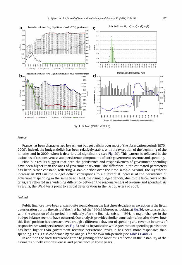
Fig. 3. Finland (1970:1–2009:3).


France

France has been characterized by resilient budget deficits overmost of the observationperiod (1970–2009). Indeed, the budget deficit has been relatively stable, with the exception of the beginning of thenineties and in 2009, when it deteriorated significantly (see Fig. 2d). This pattern is reflected in theestimates of responsiveness and persistence components of both government revenue and spending.

First, our results suggest that both the persistence and responsiveness of government spendinghave been higher than the ones of government revenue. The difference in the estimated parametershas been rather constant, reflecting a stable deficit over the time sample. Second, the significantincrease in 1993 in the budget deficit corresponds to a substantial increase of the persistence ofgovernment spending in the same year. Third, the rising budget deficits, due to the fiscal costs of thecrisis, are reflected in a widening difference between the responsiveness of revenue and spending. Asa results, the Wald tests point to a fiscal deterioration in the last quarters of 2009.

Finland

Public finances have been always quite sound during the last three decades (an exception is the fiscaldeterioration during the crisis of the first half of the 1990s).Moreover, looking at Fig. 3d, we can see thatwith the exception of the period immediately after the financial crisis in 1991, no major changes in thebudget balance seem to have occurred. Our analysis provides similar conclusions, but also shows howthis fiscal position has been achieved trough a different behaviour of spending and revenue in terms ofresponsiveness andpersistence (see Fig. 3a andb). Inparticular,while government spendingpersistencehas been higher than government revenue persistence, revenue has been more responsive thanspending. This is also confirmed by the analysis for the two sub-periods (see Tables 1 and 2).

In addition the fiscal turbulence at the beginning of the nineties is reflected in the instability of theestimates of both responsiveness and persistence in those years.


Germany

The pattern of the budget balance depicted in Fig. 4d suggests that fiscal balances have been quitestable in the last threedecades. Thishypothesishasbeenconfirmedbyouranalysis. In fact, as it is possibleto see by the joint and the single tests (see Fig. 4a–c), the difference, both in terms of responsiveness andpersistence, between government spending and revenue is not statistically significant for most of thesample period. Nevertheless, it is interesting to observe that the fiscal consolidation that occurred in the1990s has been notably related to a higher responsiveness and persistence of government revenue.

Italy

Budget deficits have been considerably high and increasing during the 1970s and the 1980s, andonly started decreasing after the beginning of the 1990s (see Fig. 5d). Our analysis, which starts in1980:1, uncovers empirical evidence for fiscal consolidation in the period after the Maastricht Treaty(see Table 2). Moreover, from the analysis of the coefficients and the associated Wald tests, we canargue that fiscal improvements in the second half of the 1990s have been achieved rather trough higherrevenue responsiveness (see Fig. 5b). Indeed, the null hypothesis of identical government revenue andspending responsiveness is mostly rejected after 1997.

Netherlands

Fiscal balances have improved in the Netherlands in the 1990s, after some deterioration in the1980s. This is (partly) captured by our analysis, which suggests that fiscal consolidation has been drivenby higher persistence of government revenue. In particular, looking at the pattern of the estimates ofresponsiveness and persistence, we can see that around 1996 government revenue has become morepersistent than government spending, after several years where the situation was the opposite (see

Fig. 4. Germany (1979:1–2009:3).

Fig. 5. Italy (1980:1–2009:3).

Fig. 6. Netherlands (1977:1–2009:3).



Fig. 6a). In contrast, regarding responsiveness, government revenue and spending do not seem to havediffered in statistically significant terms after 1999 (see Fig. 6b), when spending responsivenessdecreased and the budget position improved (see Fig. 6d).

Spain

Analyzing the pattern for fiscal budget balances in Spain, we can see that there has beena process of fiscal consolidation from 1995 onwards. In fact the budget deficit passed from above6% of GDP in 1995 to a surplus of 2.3% of GDP in 2007. Our analysis points out that the fiscalconsolidation has been driven by the higher responsiveness of government revenue than ofgovernment spending. Although we are using a short-period sample, the analysis also suggestssome recent changes in fiscal developments. Indeed, government revenue responsiveness(which has been the driver of the fiscal consolidation) seems to have decreased significantly atthe end of the sample period, while the responsiveness of government spending was stable,implying fiscal deterioration (Fig. 7).

United Kingdom

Fiscal balances in the UK have been quite stable, with the debt-to-GDP ratio decreasing throughoutthe 1970s and 1980s (see Fig. 8d). In particular, except for 2000 and 2001 (due to relatively high GDPgrowth), and in 2009 (related to the crisis), it is possible to argue that there were not significantchanges towards fiscal improvement or deterioration. This was mainly due to the fact that highergovernment spending and revenue showed a very similar behaviour in terms of persistence andresponsiveness (see Fig. 8a and b). Regarding the most recent years and in view of the widening budgetdeficit due to the crisis, our analysis signals possible fiscal tensions, as reflected in the joint Wald test

Fig. 7. Spain (1985:1–2009:3).

Fig. 8. United Kingdom (1955:2–2009:2).

Fig. 9. United States (1967:2–2009:2).



that decreases markedly. This result is mainly due to a reduction of the responsiveness of governmentrevenue to the economic cycle, therefore, reflecting a deterioration of the capacity of fiscal policy to useautomatic stabilizers to counteract the negative effects of the crisis.

US

Similarly to the UK, the fiscal balances in the US have been quite stable, although in deficit, with animprovement of the fiscal position between 1992 and 2000 (see Fig. 9d). Overall, it is possible to arguethat there has not been any significant long-term change towards fiscal consolidation or deterioration.In addition, the somewhat stable budget deficit seems to be driven by the higher persistence ofgovernment spending vis-à-vis government revenue, which is partially offset by the higher respon-siveness of government spending. The recent increase of the budget deficit, as a result of the economicand financial crisis, is reflected in the significant drop in the responsiveness of government revenue.

5. Conclusion

In this work, we propose a new approach to assess long-term fiscal developments. By analyzing thetime-varying behaviour of the two components of government spending and revenue – that is,responsiveness and persistence –, we are able to infer about the sources of fiscal deterioration and/orfiscal improvement. Drawing on quarterly data we use a Three-Stage Least Square method and recur-sively estimate those components within a system of government revenue and spending equations.

The estimates of responsiveness and persistence reveal significant changes in fiscal positions(including those related to the crises).

Nevertheless, and in general, the fiscal position has not significantly changed for Finland, France,Germany, the United Kingdom and the US – apart from the more recent years in the sample (the 2009financial crisis) – whilst it has improved moderately for Belgium, Spain, Italy, and Netherlands.However, one should notice that the occurrence of the recent crisis deeply reversed the fiscalimprovements obtained prior to the crisis, as our analysis clearly highlights.

We show that for Belgium and for the Netherlands, the fiscal improvement has beenmainly driven bya higher persistence of government revenue, vis-à-vis government spending. In addition, a higherresponsivenessofgovernmentrevenuerelative togovernmentspendingwasobserved in Italy, FinlandandSpain. Additionally, for Germany and the UK, the empirical evidence suggests a similar behaviour in termsof the persistence and responsiveness components of government spending and government revenue.

As already mentioned, regarding the more recent period that encompasses the economic andfinancial crisis, our results reflect a reduction of the responsiveness of government revenue to theeconomic cycle for most countries, compared to the responsiveness of government spending. There-fore, these results signal a deterioration of the capacity of fiscal authorities to use automatic stabilizersto counteract the negative effects of the crisis.

Acknowledgements

Wearegrateful to SilviaAlbrizio andMatthijs Lof for researchassistance and to the editorMichaelMelvinfor very useful comments. NIPE and UECE are supported by FCT (Fundação para a Ciência e a Tecnologia,Portugal), financed by ERDF and Portuguese funds.

Appendix. Data description and sources

A.1. Belgium data

GDPThe source is the IMF, International Financial Statistics (series “IFS.Q.124.9.9B.B$$.Z.W.$$$”).We seasonallyadjust quarterly data using Census X12 ARIMA, and the series comprise the period 1980:1–2009:4.


Price deflatorAll variables were deflated by the GDP deflator (2005¼100). The source is the IMF, InternationalFinancial Statistics (series “IFS.Q.124.9.9B.BIP.Z.F.$$$”). We seasonally adjust quarterly data usingCensus X12 ARIMA, and the series comprise the period 1980:1–2009:4.

Government spendingThe source is the Belgium Ministry of Finance. Government spending is defined as State Governmentexpenditure on a cash basis (series “BISM.M.FJHC.BE.91”). We seasonally adjust quarterly data usingCensus X12 ARIMA, and the series comprise the period 1967:1–2009:4.

Government revenueThe source is the Belgium Ministry of Finance. Government revenue is defined as State Governmentrevenue on a cash basis (series “BISM.M.FJBC.BE.91”). We seasonally adjust quarterly data using CensusX12 ARIMA, and the series comprise the period 1967:1–2009:4.

A.2. Finland data

GDPThe source is the IMF, International Financial Statistics (series “IFS.Q.172.9.9B.B$$.Z.W.$$$”). Weseasonally adjust quarterly data using Census X12 ARIMA, and the series comprise the period 1970:1–2009:3

Price deflatorAll variables were deflated by the GDP deflator (2005¼100). The source is the IMF, InternationalFinancial Statistics (series “IFS.Q.172.9.9B.BIP.Z.F.$$”). We seasonally adjust quarterly data using CensusX12 ARIMA, and the series comprise the period 1970:1–2009:3.

Government spendingThe source is the IMF via Finnish Ministry of Finance. Government spending is defined as StateGovernment expenditure on a cash basis (series “IFS.M.17282.ZF.”). We seasonally adjust quarterlydata using Census X12 ARIMA, and the series comprise the period 1970:1–2009:3.

Government revenueThe source is the IMF via Finnish Ministry of Finance. Government revenue is defined as StateGovernment revenue on a cash basis (series “IFS.M.17281.ZF.”). We seasonally adjust quarterly datausing Census X12 ARIMA, and the series comprise the period 1970:1–2009:3.

A.3. France data

GDPData for GDP are quarterly, seasonally adjusted, and comprise the period 1970:1–2009:3. The source isthe IMF, International Financial Statistics (series “IFS.Q.132.9.9B.B$C.Z.F.$$$”).

Price deflatorAll variables were deflated by the GDP deflator (2005¼100). Data are quarterly, seasonally adjusted,and comprise the period 1970:1–2009:3. The source is the IMF, International Financial Statistics (series“IFS.Q.132.9.9B.BIR.Z.F.$$$”).

Government spendingThe source is the IMF via French Ministry of Finance. Government spending is defined as StateGovernment expenditure on a cash basis (series “IFS.M.13282z.ZF.”). We seasonally adjust quarterlydata using Census X12 ARIMA, and the series comprise the period 1970:1–2009:3.


Government revenueThe source is the IMF via French Ministry of Finance. Government revenue is defined as StateGovernment revenue on a cash basis (series “IFS.M.13281.ZF.”). We seasonally adjust quarterly datausing Census X12 ARIMA, and the series comprise the period 1970:1–2009:3.

A.4. Germany data



Government spendingThe source is the Bundesbank and the Monthly Reports released by the German Ministry of Finance.Government spending is defined as general government total expenditure on a cash basis. Weseasonally adjust quarterly data using Census X12 ARIMA, and the series comprise the period1979:1–2009:3.

Government revenueThe source is the Bundesbank and the Monthly Reports released by the German Ministry of Finance.Government revenue is defined as general government total revenue on a cash basis. We seasonallyadjust quarterly data using Census X12 ARIMA, and the series comprise the period 1979:1–2009:3.

A.5. Italy data



Government spendingThe source is the Bank of Italy and the Italian Ministry of Finance. Government spending is defined asCentral Government primary expenditure on a cash basis. We seasonally adjust quarterly data usingCensus X12 ARIMA, and the series comprise the period 1960:1–2009:3.

Government revenueThe source is the Bank of Italy and the Italian Ministry of Finance. Government revenue is defined ascentral government total revenue on a cash basis. We seasonally adjust quarterly data using CensusX12 ARIMA, and the series comprise the period 1960:1–2009:3.

A.6. Spain data




Government spendingThe source is the IMF via Spanish Ministry of Finance. Government spending is defined as StateGovernment expenditure on a cash basis (series “IFS.M.18482.Zf.”). We seasonally adjust quarterlydata using Census X12 ARIMA, and the series comprise the period 1985:1–2009:3.

Government revenueThe source is the IMF via Spanish Ministry of Finance. Government Revenue is defined as StateGovernment revenue on a cash basis (series “IFS.M.18481.Zf.”). We seasonally adjust quarterly datausing Census X12 ARIMA, and the series comprise the period 1985:1–2009:3.

A.7. Netherlands data

GDPThe source is the IMF, International Financial Statistics (series “IFS.Q.138.9.9B.B$C.Z.W.$$$”).Weseasonallyadjust quarterly data using Census X12 ARIMA, and the series comprise the period 1970:1–2009:3.

Price deflatorAll variables were deflated by the GDP deflator (2005¼100). The source is the IMF, InternationalFinancial Statistics (series “IFS.Q.138.9.9B.BIR.Z.F.$$$”). We seasonally adjust quarterly data usingCensus X12 ARIMA, and the series comprise the period 1970:1–2009:3.

Government spendingThe source is the IMF via Dutch Ministry of Finance. Government spending is defined as StateGovernment expenditure on a cash basis (series “IFS.M.138.C.C2.$$$.C.G.$$$”). We seasonally adjustquarterly data using Census X12 ARIMA, and the series comprise the period 1977:1–2009:3.

Government revenueThe source is the IMF via Dutch Ministry of Finance. Government revenue is defined as StateGovernment revenue on a cash basis (series “IFS.M.138.C.C1.$$$.C.G.$$$”). We seasonally adjustquarterly data using Census X12 ARIMA, and the series comprise the period 1977:1–2009:3.

A.8. UK data

GDPData for GDP are quarterly, seasonally adjusted, and comprise the period 1955:1–2009:2. The source isthe Office for National Statistics, Release UKEA, Table A1 (series “YBHA”).

Price deflatorAll variables were deflated by the GDP deflator. Data are quarterly, seasonally adjusted, and comprisethe period 1955:1–2009:2. The source is the Office for National Statistics, Release MDS, Table 1.1 (series“YBGB”).

Government spendingThe source is the Office for National Statistics (ONS), Release Public Sector Accounts. Governmentspending is defined as total current expenditures of the Public Sector ESA 95 (series “ANLT”) less netinvestment (series “ANNW”). We seasonally adjust quarterly data using Census X12 ARIMA, and theseries comprise the period 1947:1–2009:2.


Government revenueThe source is the Office for National Statistics (ONS), Release Public Sector Accounts. Governmentrevenue is defined as total current receipts of the Public Sector ESA 95 (series “ANBT”). We seasonallyadjust quarterly data using Census X12 ARIMA, and the series comprise the period 1947:1–2009:2.

A.9. US data

GDPThe source is Bureau of Economic Analysis, NIPA Table 1.1.5, line 1. Data for GDP are quarterly,seasonally adjusted, and comprise the period 1947:1–2009:3.

Price deflatorAll variables were deflated by the GDP deflator. Data are quarterly, seasonally adjusted, and comprisethe period 1967:1–2009:3. The source is the Bureau of Economic Analysis, NIPA Tables 1.1.5 and 1.1.6,line 1.

Government spendingThe source is Bureau of Economic Analysis, NIPA Table 3.2. Government spending is defined as totalFederal Government Current Expenditure (line 39). Data are quarterly, seasonally adjusted, andcomprise the period 1960:1–2009:2.

Government revenueThe source is Bureau of Economic Analysis, NIPA Table 3.2. Government revenue is defined asgovernment receipts at annual rates (line 36). Data are quarterly, seasonally adjusted, and comprise theperiod 1947:1–2009:2.

References

Afonso, A., 2005. Fiscal sustainability: the unpleasant European case. FinanzArchiv 61 (1), 19–44.Afonso, A., 2008. Ricardian fiscal regimes in the European Union. Empirica 35 (3), 313–334.Afonso, A., Rault, C., 2008. 3-Step analysis of public finances sustainability: the case of the European Union. ECB working paper

no. 908.Afonso, A., Rault, C., 2010. What do we really know about fiscal sustainability in the EU? A panel data diagnostic. Review of

World Economics 125 (4), 731–755.Afonso, A., Agnello, Furceri, D., 2010. Fiscal policy responsiveness, persistence and discretion. Public choice, forthcoming.Ahmed, S., Rogers, J., 1995. Government budget deficits and trade deficits. Are present value constraints satisfied in long-term

data? Journal of Monetary Economics 36, 351–374.Baglioni, A., Cherubini, U., 1993. Intertemporal budget constraint and public debt sustainability: the case of Italy. Applied

Economics 25, 275–283.Bohn, H., 2007. Are stationarity and cointegration restrictions really necessary for the intertemporal budget constraint? Journal

of Monetary Economics 54 (7), 1837–1847.Fatás, A., Mihov, I., 2003. The case for restricting fiscal policy discretion. Quarterly Journal of Economics 118, 1419–1447.Fatás, A., Mihov, I., 2006. The macroeconomics effects of fiscal rules in the US states. Journal of Public Economics 90, 101–117.Hakkio, G., Rush, M., 1991. Is the budget deficit too large? Economic Inquiry 29, 429–445.Hamilton, J., Flavin, M., 1986. On the limitations of government borrowing: a framework for empirical testing. American

Economic Review 76, 808–816.Hatemi-J, A., 2002. Fiscal policy in Sweden: effects of EMU criteria convergence. Economic Modelling 19, 121–136.Haug, A., 1995. Has federal budget deficit policy changed in recent years? Economic Inquiry 33, 104–118.MacDonald, R., 1992. Some tests of the government’s intertemporal budget constraint using U.S. data. Applied Economics 24,

1287–1292.Onorante, L., Pedregal, D., Pérez, J., Signorini, S., 2008. The usefulness of infra-annual government cash budgetary data for fiscal

forecasting in the euro area. ECB working paper no. 901.Quintos, C., 1995. Sustainability of the deficit process with structural shifts. Journal of Business & Economic Statistics 13,

409–417.Smith, G., Zin, S., 1991. Persistent deficits and the market value of government debt. Journal of Applied Econometrics 6, 31–44.Trehan, B., Walsh, C., 1988. Common trends, the government’s budget constraint, and revenue smoothing. Journal of Economic

Dynamics and Control 12, 425–444.Trehan, B., Walsh, C., 1991. Testing intertemporal budget constraints: theory and applications to U.S. federal budget and current

account deficits. Journal of Money, Credit, and Banking 23, 206–223.Zellner, A., Theil, H., 1962. Three stage least squares: simultaneous estimation of simultaneous equations. Econometrica 30 (1),

54–78.

Assessing long-term fiscal developments: A new approach

Documents

Transcript of Assessing long-term fiscal developments: A new approach