Assessing Land Use and Regulations

in Rural

King County, WA*

*Prepared April 29,2014 for website

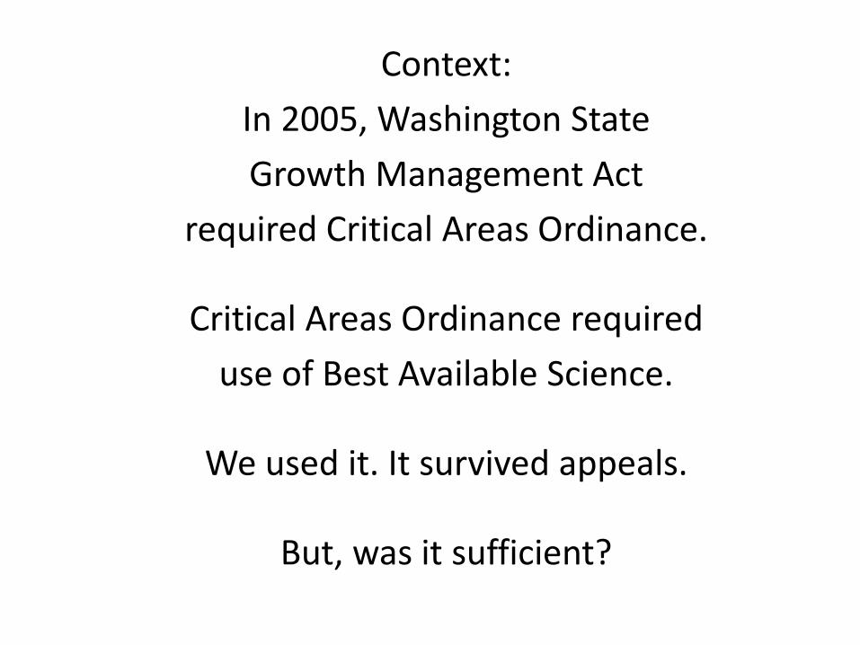
Context: In 2005, Washington State Growth Management Act

required Critical Areas Ordinance.

Critical Areas Ordinance required use of Best Available Science.

We used it. It survived appeals.

But, was it sufficient?

Critical Areas Ordinances (CAO)*

K.C.C. 21A Critical Areas Zoning code (Ord. 15051) K.C.C. 16.82

Clearing & Grading (Ord. 15053)

K.C.C. 16.82 Stormwater (Ord. 15052)

Best Available Science: *Also have non-regulatory measures, e.g., stewardship and tax incentive programs,

acquisitions, transfer of development rights, and habitat restoration projects

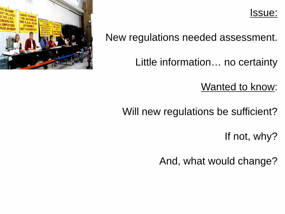
Issue:

New regulations needed assessment.

Little information… no certainty

Wanted to know:

Will new regulations be sufficient?

If not, why?

And, what would change?

To find out, we: – built an experimental framework,

and – conducted an experiment.

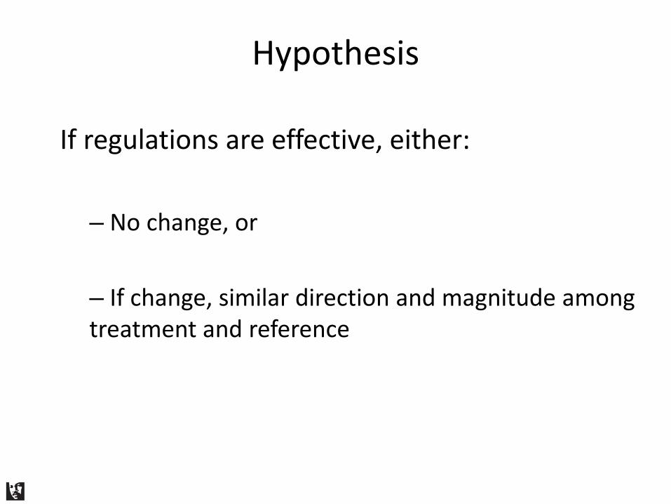
Hypothesis

If regulations are effective, either:

– No change, or

– If change, similar direction and magnitude among treatment and reference

Key Questions:

• Did the environment change (respond)? If so, was it related to CAO implementation?

• If response, how might the CAO be modified? • How well were regulations followed?

• Did non-compliance have an effect?

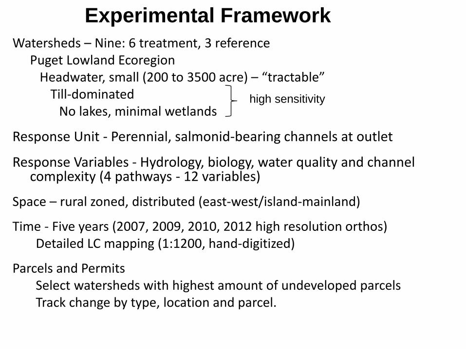
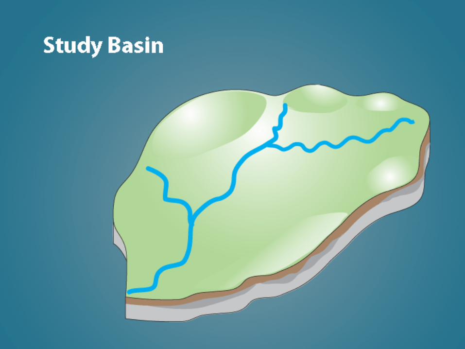
Watersheds – Nine: 6 treatment, 3 reference Puget Lowland Ecoregion Headwater, small (200 to 3500 acre) – “tractable”

Till-dominated No lakes, minimal wetlands

Response Unit - Perennial, salmonid-bearing channels at outlet

Response Variables - Hydrology, biology, water quality and channel complexity (4 pathways - 12 variables)

Space – rural zoned, distributed (east-west/island-mainland)

Time - Five years (2007, 2009, 2010, 2012 high resolution orthos) Detailed LC mapping (1:1200, hand-digitized)

Parcels and Permits Select watersheds with highest amount of undeveloped parcels Track change by type, location and parcel.

Experimental Framework

high sensitivity

and… a priori design:

– BACI w/ multiple sites & response indicators

– Time and Space (no space-for-time substitution)

– Statistically strong to minimize Type II Error (likelihood of concluding no effect when, in fact, there was one)

Assessed history (legacies)

Reference scenarios: historic, full build-out (worst-case) and urban

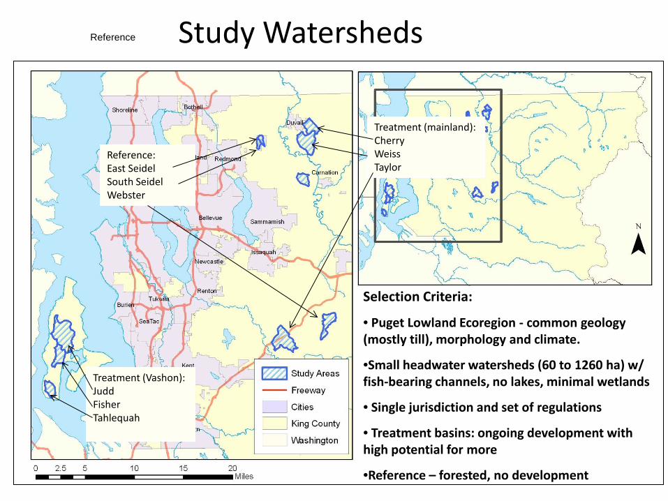
Study Watersheds

Treatment (Vashon): Judd Fisher Tahlequah

Reference: East Seidel South Seidel Webster

Treatment (mainland): Cherry Weiss Taylor

Selection Criteria:

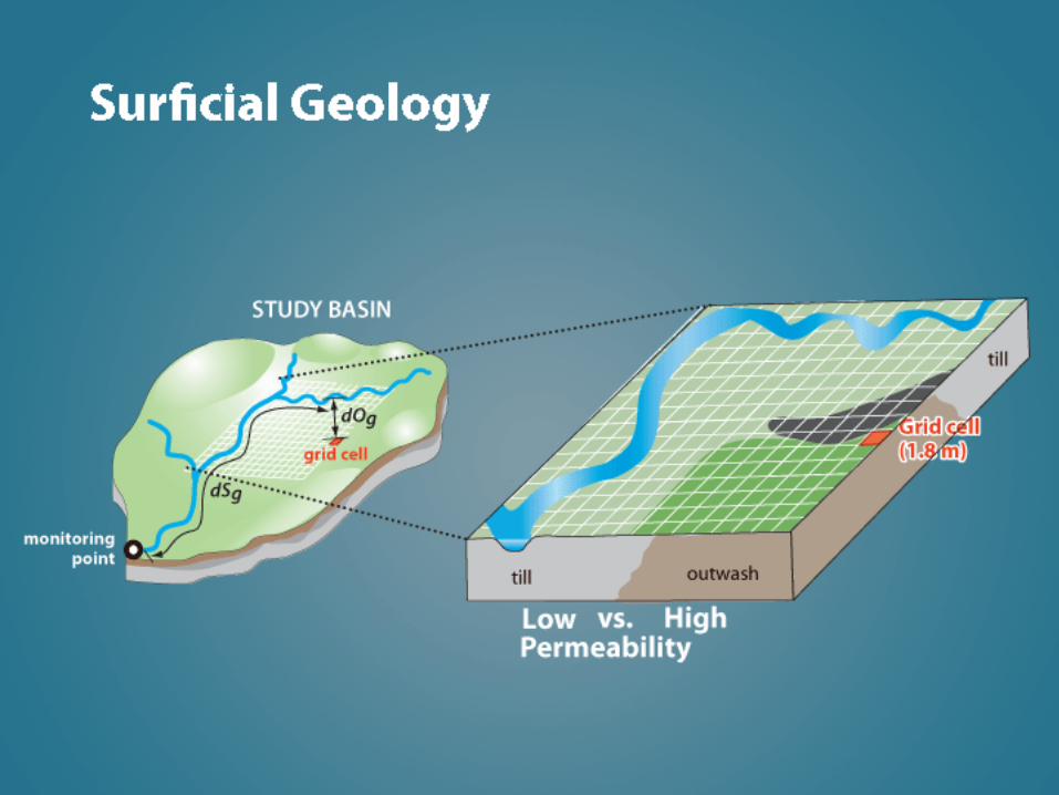
• Puget Lowland Ecoregion - common geology (mostly till), morphology and climate.

•Small headwater watersheds (60 to 1260 ha) w/ fish-bearing channels, no lakes, minimal wetlands

• Single jurisdiction and set of regulations

• Treatment basins: ongoing development with high potential for more

•Reference – forested, no development

Reference

Measuring Environmental Response

Hydrology – High Pulse Counts

Biology Macro-invertebrates BIBI

Water Quality Conductivity, Temperature

Channel Complexity Reach-Averaged Velocity (salt tracers) EMAP – substrate, thalweg, pools, LWD

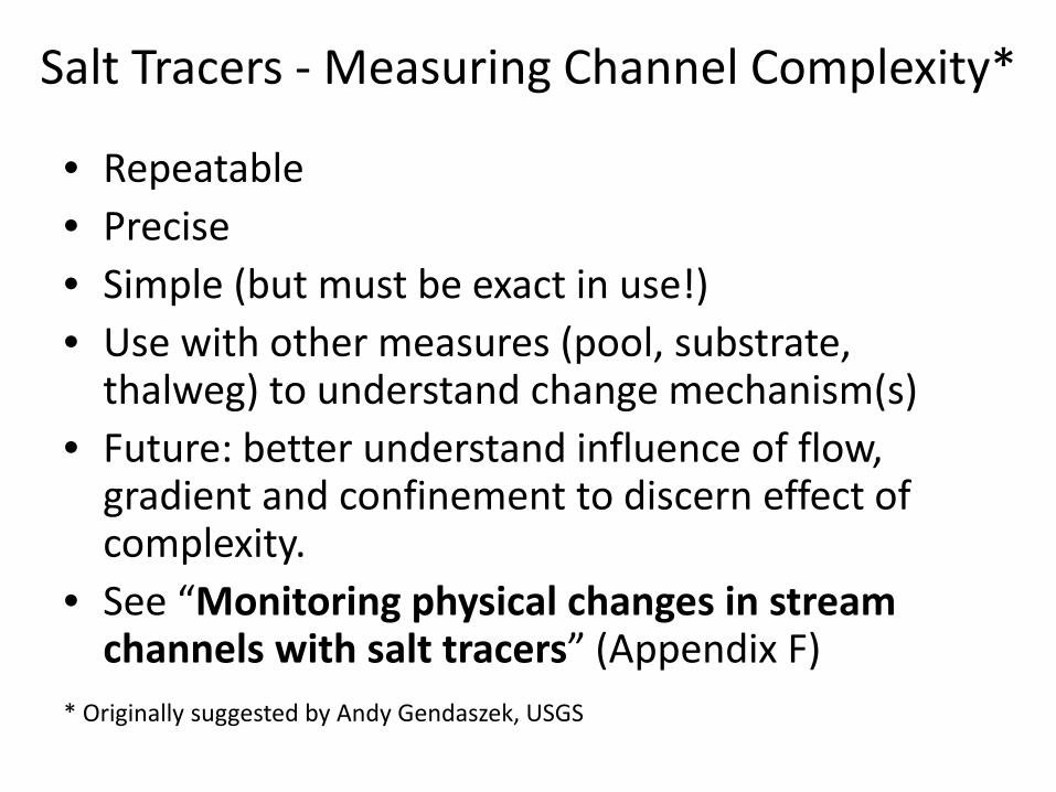
Salt Tracers - Measuring Channel Complexity*

• Repeatable • Precise • Simple (but must be exact in use!) • Use with other measures (pool, substrate,

thalweg) to understand change mechanism(s) • Future: better understand influence of flow,

gradient and confinement to discern effect of complexity.

• See “Monitoring physical changes in stream channels with salt tracers” (Appendix F)

* Originally suggested by Andy Gendaszek, USGS

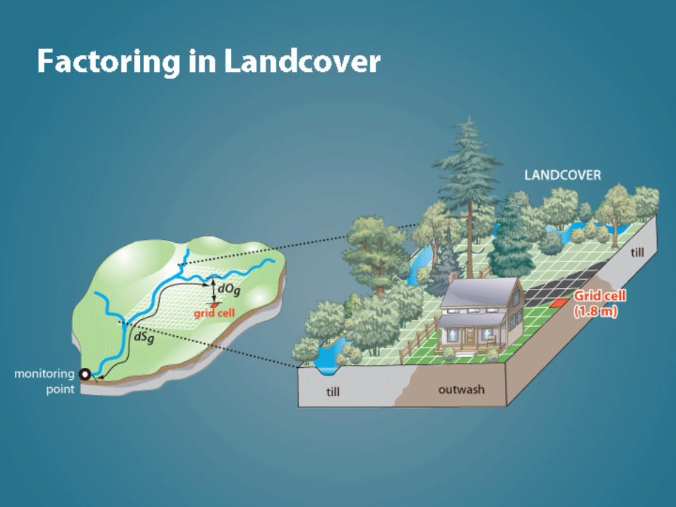
Measuring Land Cover change as “treatment”

0

100

200

300

400

500

600

700

2000 2001 2002 2003 2004 2005 2006 2007 2008 2009 2010 2011 2012 2013*

Dwelling-Single

Dwelling-Modular

Dwelling-Mobile

Basic

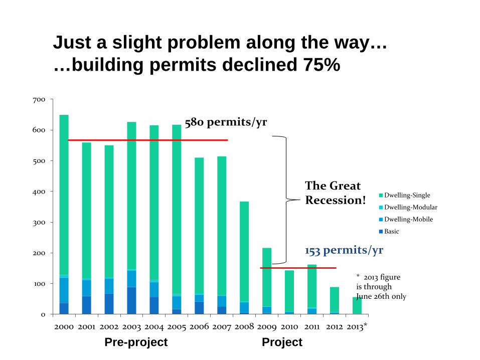
* 2013 figure is through June 26th only

580 permits/yr

The Great Recession!

Just a slight problem along the way… …building permits declined 75%

153 permits/yr

Pre-project Project

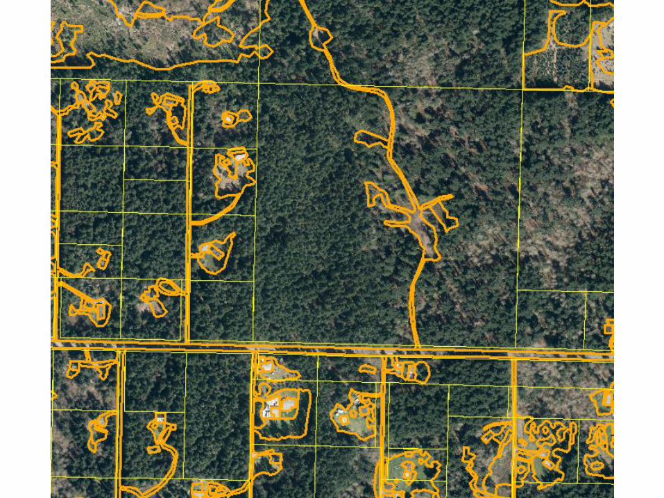
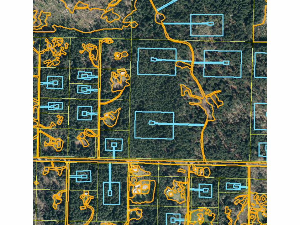
Land Cover Scenarios (putting the present in perspective) •Project (2007 – 2012) – hand-digitized land covers, high resolution (0.3 m) orthophotos (2007, 2009, 2010, 2012)

•Historic (~1900 to 2007) – are there “Ghosts of land use past” (Harding et al 1998)? Used reports and maps, aerial photos, satellite (see Michalak et al 2013 Appendix D) • Full Build-out – possible “worst case”? Apply development footprint on undeveloped parcels to assess potential change. •Urban – 2007 Juanita Creek

The Past - Data Timeline*

All Basins

Land Cover 30 m pixels

1965 1936

Vashon and

Control

1948

Aerials

All Basins

1911 1907-08

Timber

Cruise

Soil Survey

Vashon Eastern and

Control

*Michalak e t al. 2013.

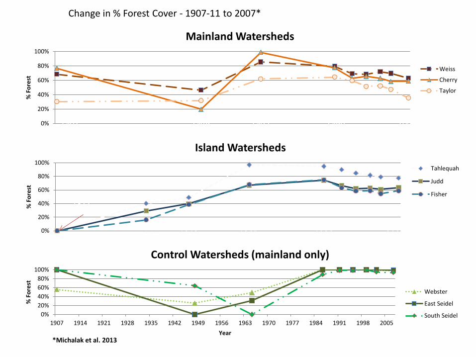
Change in % Forest Cover - 1907-11 to 2007*

0%

20%

40%

60%

80%

100%

% F

ores

t Mainland Watersheds

Weiss

Cherry

Taylor

0%

20%

40%

60%

80%

100%

% F

ores

t

Island Watersheds

Tahlequah

Judd

Fisher

0%20%40%60%80%

100%

1907 1914 1921 1928 1935 1942 1949 1956 1963 1970 1977 1984 1991 1998 2005

% F

ores

t

Year

Control Basins

Webster

East Seidel

South Seidel

1907 1948 1965 1986 2007

1911

1948 1965 1986 2007 1936

0%20%40%60%80%

100%

1907 1914 1921 1928 1935 1942 1949 1956 1963 1970 1977 1984 1991 1998 2005

% F

ores

t

Year

Control Watersheds (mainland only)

Webster

East Seidel

South Seidel

*Michalak et al. 2013

Estimating the

Future Condition

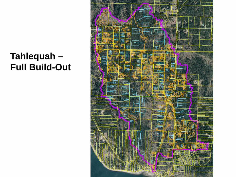
Tahlequah – Full Build-Out

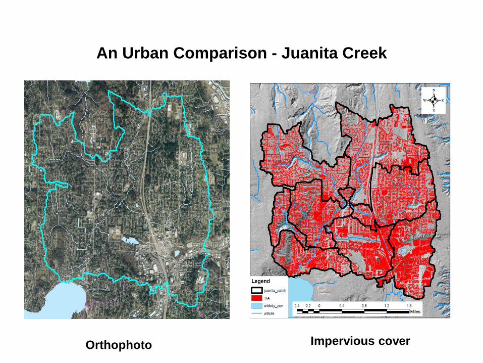
An Urban Comparison - Juanita Creek

Orthophoto Impervious cover

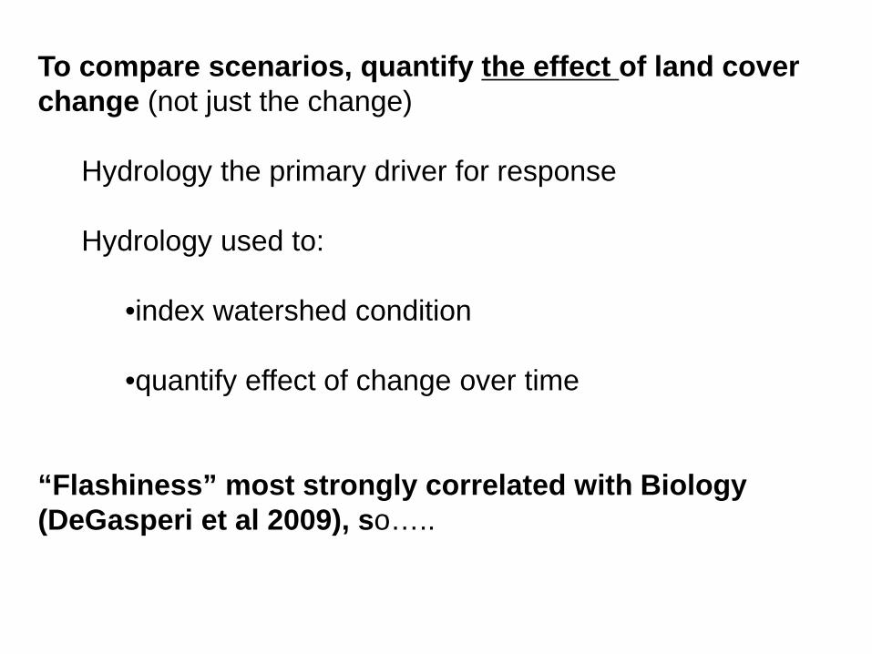
To compare scenarios, quantify the effect of land cover change (not just the change)

Hydrology the primary driver for response Hydrology used to:

•index watershed condition

•quantify effect of change over time “Flashiness” most strongly correlated with Biology (DeGasperi et al 2009), so…..

Pre-development Post-development

High Pulse Counts*

* From Horner 2013

High Pulse Counts* Effect of geology and land cover

* Modeled 61-year averages for pre-existing watershed models used to model the HCI

accounting for land cover, geology and distance

CAUTION

SPATIALLY

EXPLICIT CONTENT

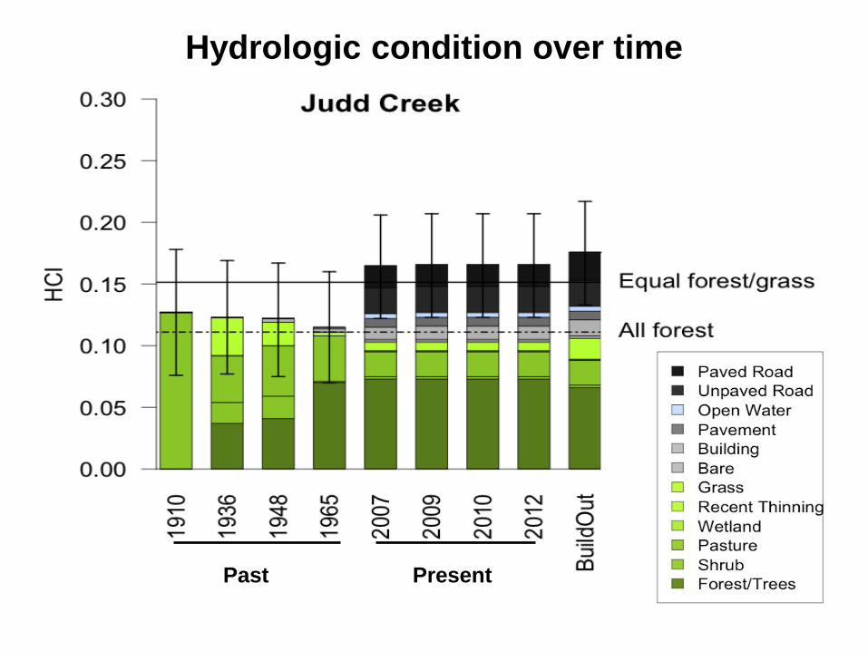
HCI = watershed hydrologic condition measuring stick

Accounts for spatial configuration of

land covers and geology

X-axis - improved precision

Models used to estimate HPCs :

•Accuracy fair (r2 ≥ 0.6) to excellent (r2 ≥0.9) for in simulating hourly flow rates and HPCs, •are being used for other major assessments (e.g., WRIA 9 Stormwater Retrofit Planning)

•are BAS

Model accuracy and utility

Average Watershed HCI Average Regulatory Stream Buffer HCI

r p-value r p-value Watershed Percent Impervious 0.94 <0.01 0.68 0.07 Watershed Percent Forest -0.91 <0.01 -0.58 0.12 Average Watershed HCI - - 0.71 0.06 Average Regulatory Stream Buffer HCI 0.71 0.06 - - Ratio of watershed and buffer HCIs 0.05 0.46 -0.66 0.08 High Pulse Count 0.88 0.01 0.96 <0.01 Average Annual Temp at Baseflow 0.20 0.36 0.6 0.10 Conductivity at Baseflow 0.08 0.44 -0.24 0.33 Percent Pool Length of Thalweg 0.44 0.19 -0.03 0.96 CV of Thalweg Depth -0.44 0.19 -0.55 0.13 Average Velocity at MAD 0.36 0.24 0.85 0.02 Average Residual Pool Depth 0.08 0.44 0.68 0.07 Large Wood per 100m 0.64 0.09 0.55 0.13 Percent Silt and Sand -0.36 0.24 -0.78 0.03 BIBI 0.42 0.21 0.56 0.12 X7DADMax 0.94 <0.01 0.68 0.07

Project timeframe averages for six treatment watersheds

Putting it all together

Present Past

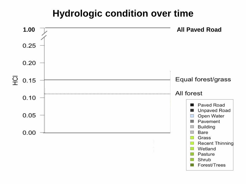
Hydrologic condition over time 1.00 1.00 All Paved Road

Present Past

Hydrologic condition over time 1.00 1.00 All Paved Road

Present Past

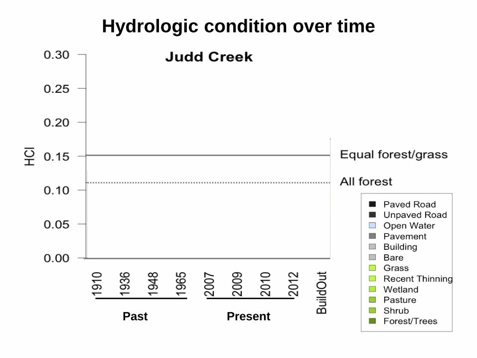
Hydrologic condition over time

Present Past

Hydrologic condition over time

Present Past

Hydrologic condition over time

Present Past

Hydrologic condition over time

Present Past

Hydrologic condition over time

“Worst Case”

Least Most Level of current development

Treatment Watersheds

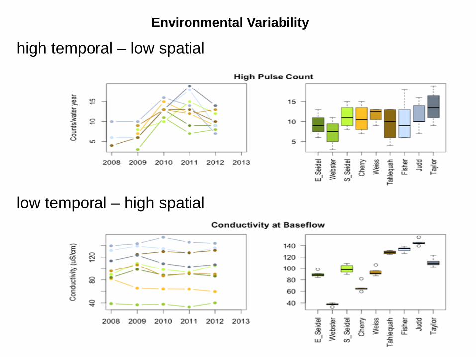
low temporal – high spatial

high temporal – low spatial

Environmental Variability

Environmental Response?

No change except,

Two (secondary) habitat variables –

•thalweg length & % Pool

•But, in opposite direction predicted if CAO not effective, and

•both subject to high measurement error.

Juanita Creek (urban) comparison

1.2Xs = largest change 2012 and FBO

3.9Xs > Taylor Creek at FBO

1.2Xs = largest change between 2012 and FBO

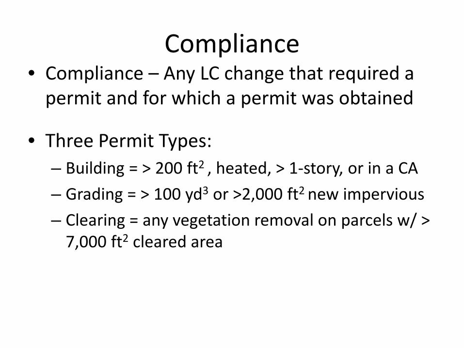
Compliance • Compliance – Any LC change that required a

permit and for which a permit was obtained

• Three Permit Types: – Building = > 200 ft2 , heated, > 1-story, or in a CA – Grading = > 100 yd3 or >2,000 ft2 new impervious – Clearing = any vegetation removal on parcels w/ >

7,000 ft2 cleared area

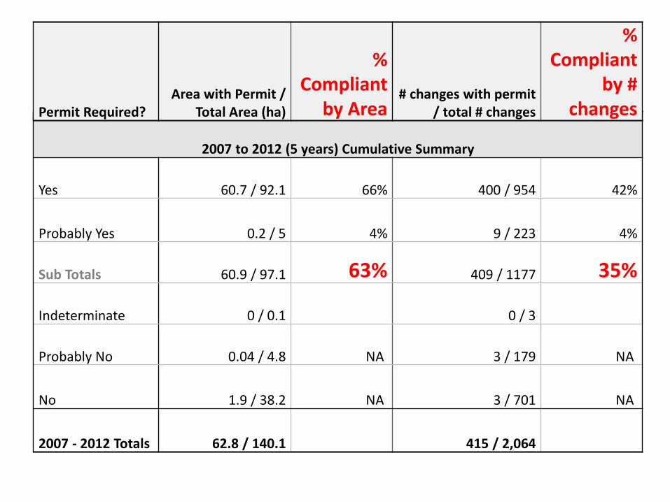
2007 to 2012 (5 years) Cumulative Summary

Yes 60.7 / 92.1 66% 400 / 954 42%

Probably Yes 0.2 / 5 4% 9 / 223 4%

Sub Totals 60.9 / 97.1 63% 409 / 1177 35%

Indeterminate 0 / 0.1 0 / 3

Probably No 0.04 / 4.8 NA 3 / 179 NA

No 1.9 / 38.2 NA 3 / 701 NA

2007 - 2012 Totals 62.8 / 140.1 415 / 2,064

Permit Required? Area with Permit /

Total Area (ha)

% Compliant

by Area # changes with permit

/ total # changes

% Compliant

by # changes

Extent

Area (ha)

% area with no

LC change

% area with LC change*

% area with Compliant LC change

% area with Non- compliant

LC Change

Watershed 4105 96.6% 3.4% 2.4% 1.0%

Regulatory Stream Buffer

417 99.3% 0.7% 0.5% 0.2%

Land cover change over 5-years

Compliance rate not great but area was small.

r2 = 0.15, p = 0.03

Buildings Clearing and Grading

r2 = 0.64, p<0.01

Compliance by Area and Permit Type

No permit needed:

•if outside a regulatory buffer

•only to extent necessary to remove the hazard Turns out…

- ~ 25% of forest cover removal within 150’ (~ one site-potential-tree-height) of a building -In three watersheds (Judd, Taylor and Fisher), 75% of forest cover loss w/in 1 SPTH of a building

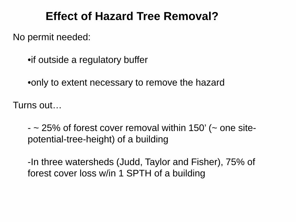
Effect of Hazard Tree Removal?

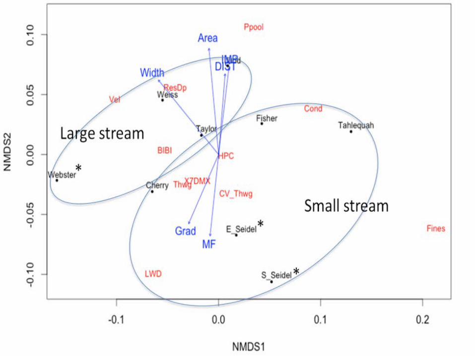
Ordination

• Exploratory – “Putting things in order”

• Squeezing three dimensions into two

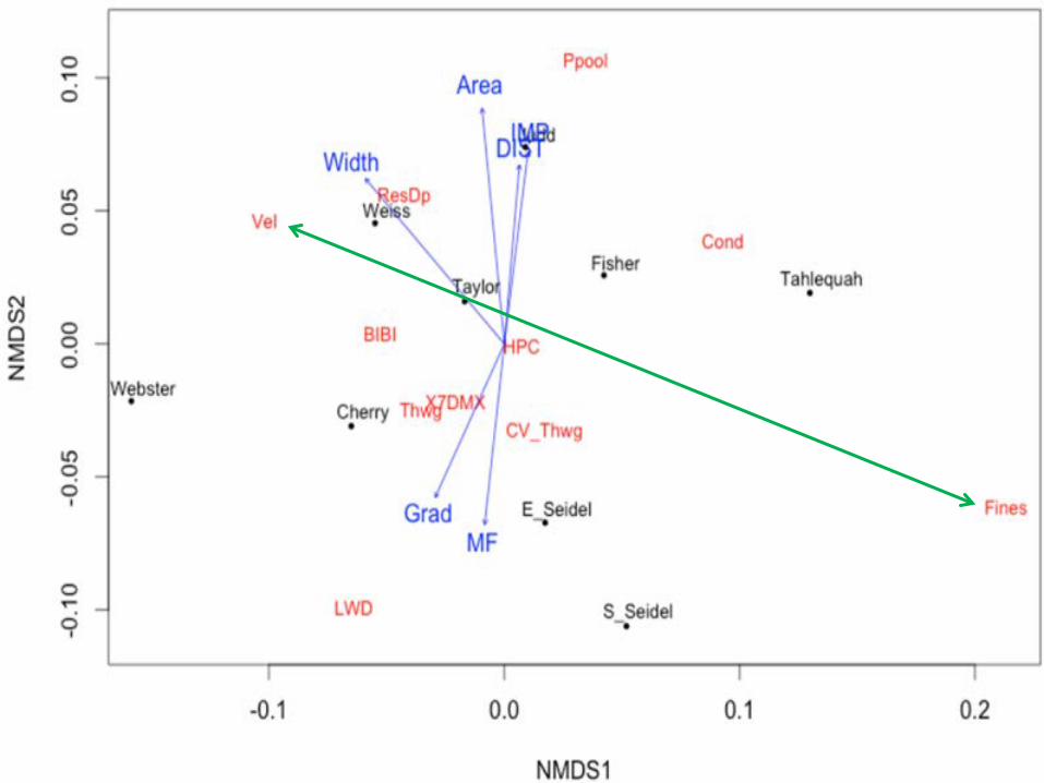
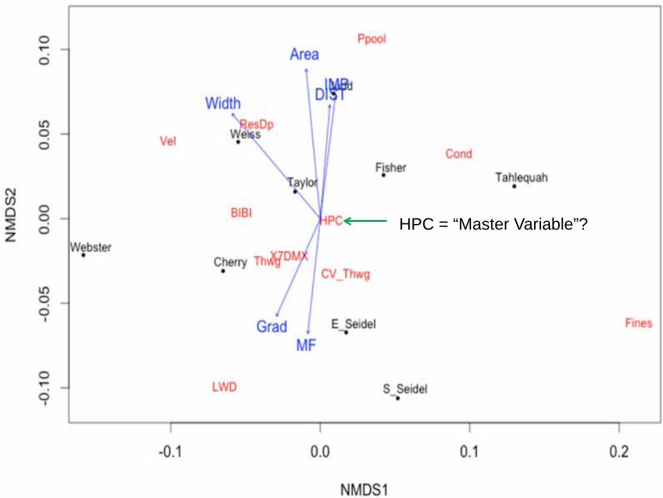
HPC = “Master Variable”?

Conclusions,

Recommendations,

Additional value

Are regulations effective?

To say definitively – more treatment and/or time needed

HCIs suggest:

• Small change over time among rural scenarios, and

• Urban much worse than rural worst case.

Study provides:

• Valuable baseline and new information

• Indication that regulations may be protective of watershed hydrology, and

• May facilitate restoration – not likely to be undone by degrading watershed.

Compliance? Was it a problem?

Could be better.

Still, o no detectable effect of non-compliance (rates high, but

actual area affected was small)

o no observed rampant or egregiously bad actions, and

o regulatory stream buffers much less affected/better condition

Should the CAO be modified? No change recommended - no obvious problem

so no basis

Follow-up/future work? Assess more treatment and/or time in the study

watersheds. Apply framework elsewhere in PS Lowland

Ecoregion

Prevention of Toxics? Protection of Wildlife?

Potential Additional Uses

• “Watershed Laboratory” - nine “wired” watersheds

• HCI – no need to build expensive hydrology models

everywhere

Potential Additional Uses (cont.) • Ordination –

– Structuring study designs and databases – Hypothesis testing

• Time and Space Analyses – historic, current, future conditions analyses – parcel-based assessment could be nested in reach

and watershed scale

• Tracers – – precise assessment of channel change – Improved understanding of eco-hydraulics

Summary – What we did LC Change – Present, Past and Future Environmental Response – Four Pathways,

standard metrics plus tracers

Permitting and Compliance – How much?

Website and Final Report:http://www.kingcounty.gov/environment/data-and-trends/monitoring-data/critical-areas.aspx

Acknowledgements : 11 groups – over 60 people! Funders: USEPA & King County Tech Collaborators: EPA (Jayshika Ramrakha, Tony Fournier, Gretchen Hayslip,

Krista Mendelman, Mike Rylko, John Gabrielson), UW UERL (Marina Alberti,

Julia Michalak), USGS (Christian Torgersen, Rich Sheibley, Andrew Gendaszek,

Bob Black), Assistance: WDOE (Stephen Stanley) VCC, GRCC GIS Lab, KC Interns KC Project Team:

DNRP – Gino Lucchetti (Project Manager), Josh Latterell, Ray Timm, Leska Fore, Jennifer Vanderhoof, Jeff Burkey, Dan Smith (gaging), Dan Smith (database), Charlie Zhen, David Funke, Stephanie Hess, Jo Wilhelm, Chris Gregersen, Chris Knutson, Ken Rauscher, Bob Fuerstenberg (ret.), Klaus Richter (ret.)

DDES - Harry Reinert, Paul McCombs, Jon Petersen, Steve Bottheim, Betsy MacWhinney, Pesha Klein