Carlos Pestana Barros & Nicolas Peypoch

A Comparative Analysis of Productivity Change in Italian and Portuguese Airports

WP 006/2007/DE _________________________________________________________

António Afonso and Sónia Fernandes

Assessing Hospital Efficiency: Non-parametric Evidence for Portugal

WP 07/2008/DE/UECE _________________________________________________________

Department of Economics

WORKING PAPERS

ISSN Nº 0874-4548

School of Economics and Management TECHNICAL UNIVERSITY OF LISBON

Assessing Hospital Efficiency: Non-parametric

Evidence for Portugal *

António Afonso # and Sónia Fernandes $

February 2008

Abstract

We compute DEA efficiency scores and Malmquist indexes for a panel data set comprising 68 Portuguese public hospitals belonging to the National Health System (NHS) in the period 2000-2005, when several units started being run in an entrepreneurial framework. With data on hospital services’ and resource quantities we construct an output distance function, we assess by how much can output quantities be proportionally expanded without changing input quantities Our results show that, on average, the NHS hospital sector revealed positive but small productivity growth between 2000 and 2004. The mean TFP indices vary between 0.917 and 1.109, implying some differences in the Malmquist indices across specifications. Furthermore, there are significant fluctuations among NHS hospitals in terms of individual efficiency scores from one year to the other. JEL classification: C14, C61, D24, H51, I12 Keywords: Public hospitals, Data Envelopment Analysis, Malmquist indices, Portugal

* The opinions expressed herein are those of the authors and do not necessarily reflect those of the author’s employers. # ISEG/TULisbon – Technical University of Lisbon, Department of Economics; UECE – Research Unit on Complexity and Economics, R. Miguel Lupi 20, 1249-078 Lisbon, Portugal, email: aafonso@iseg.utl.pt. UECE is supported by FCT (Fundação para a Ciência e a Tecnologia, Portugal), financed by ERDF and Portuguese funds. $ Court of Accounts, Av. da República, 65, 1069-045 Lisbon, Portugal, email: sonfer1@sapo.pt.

2

Contents

1 – Introduction .......................................................................................................................... 3

2 – Overview of the Portuguese public hospital sector .............................................................. 4

3 – Productivity measurement .................................................................................................... 8

3.1 – Literature review................................................................................................................ 8

3.2 – Malmquist Productivity Index......................................................................................... 14

4 – Empirical analysis .............................................................................................................. 18

4.1 – Data.................................................................................................................................. 18

4.2 – Model specifications........................................................................................................ 24

4.3 – Results and discussion..................................................................................................... 27

5 – Conclusion.......................................................................................................................... 34

References ................................................................................................................................ 35

3

1 – INTRODUCTION

During the period 1992-2003 Portuguese health care expenditure has rapidly increased

with the share of public spending in total health spending also increasing from 60% in

1992 to around 70% in 2003. On the other hand, under a new legal framework, the

enterprising model for the health sector was the option gradually preferred by the

Government. For instance, in the end of 2002 the legal status of 31 hospitals (40 per

cent) changed, from public institutions of the Administrative Public Sector (SPA) into

hospital enterprises (SA) with limited liabilities. Whether such changes can spur

increases in performance and efficiency regarding the services provided to the public is

then a paramount issue in a context of limited public resources.

Data Envelopment Analysis (DEA) has been widely used to calculate changes in Total

Factor Productivity within the public hospitals sector, where price data is difficult to

find and multi-output production is relevant, since it does not require the imposition of

any behavioural assumptions such as revenue maximization or cost minimization

(Lovell, 2000). DEA analysis has also been used recently to assess the efficiency of the

public sector in cross-country analysis for overall public sector efficiency analysis

(Afonso et al., 2005), and to asses local government spending efficiency (for instance

for Portugal, Afonso and Fernandes, 2006).

The aim of this paper is to estimate in a non-parametrical framework, measures of

hospital technical efficiency across 68 Portuguese hospitals belonging to the National

Health System (NHS) during the period 2000-2005. For that purpose we will use both

DEA analysis and compute Malmquist indexes. Additionally, the paper also examines

heterogeneity and efficiency resulting from the recent “privatisation” of some

Portuguese hospitals.

The paper is organised as follows. Section two gives an overview of the Portuguese

public hospital sector. Section three reviews the literature on the non-parametric

measurement of hospital efficiency and explains the analytical framework used in the

paper. Section four conducts our empirical efficiency analysis and discusses the results.

Section five concludes.

4

2 – OVERVIEW OF THE PORTUGUESE PUBLIC HOSPITAL SECTOR

Regarding the institutional framework the Portuguese National Health Care System

(NHS) was created in 1979, following the approval of the Constitution in 1976. The

health service model then put in place1 was characterized by universal coverage, equity

concerns, and financed via tax revenues. In fact, the Constitution guaranteed to all

citizens ‘the right to health’, to be provided by a universal National Health Service,

comprehensive and free of charge.

New principles were introduced in 1990 for the organization and functioning of the

health system and assigned an explicit role to the private for-profit and non-for-profit

sectors through contracting with the NHS.2 The objectives of the NHS in promoting

efficiency, quality, accountability and devolution of power were also emphasised (see

Oliveira and Pinto, 2005; Bentes et al., 2004).

In what concerns hospital care, traditionally it was a much centralised sector dominated

by public provision, and according to several authors it was characterized by

inefficiency and performed poorly in terms of cost containment.3 Recently, and

following health reform trends in other European countries, a new hospital management

law was passed through Portuguese Parliament in 2002.4 The purpose of this Law was

to “enable the changeover of some institutions into public enterprises as well as the set

up of a series of entrepreneurial principles such as freedom of choice by the patient,

budget contracting, and activity based payment of professionals” (Bentes et al., 2004,

pp. 16)).

1 According to the definition of Docteur and Oxley (2003), the Portuguese health system was put in place as a “public-integrated” model. Nowadays, this model also exists in the Nordic countries, Australia, Italy and Greece. 2 Law nº 48/90 (see Base XXIV). The reforms introduced in the 1990s have been pushing the Portuguese health system put in place in the late 1970s towards a “public-contract model”, characterized by an increased role and participation of the private sector (see Docteur and Oxley, 2003). 3 See, for example, Dixon and Mossialos (2000) and Oliveira and Pinto (2005). Oliveira (2002) argues that inefficiency arises among Portuguese public hospitals for several reasons such as: (1) the payment system to doctors, traditionally based on collective contracts, gives little incentives for productivity and results mainly in a lack of doctors in the public system; (2) hospital administrations are not encouraged to keep within budgets limits because traditionally they are not penalised for overruns; (3) hospital administrations have little autonomy in what concerns management decisions about investments and human resources. 4 Law nº 27/2002 that introduced amendments to the 1990 NHS Law.

5

There are several implications of the new hospital management law (see Lima and

Whynes, 2003). First, collective contracts were replaced by individual labour contracts,

with hospitals being now free to hire personnel and use different payment systems.5

Second, it introduced more flexibility in the NHS hospitals management structures and

allowed the coexistence of public entities with private entities acting in a cooperative

way and sharing the same objective of satisfying patient needs. Third, the traditional

concept of the “NHS hospital” was replaced by the new concept of “Network of health

care providers”, which according to article 2, nº 1 of Law nº 27/2002, includes four

types of hospitals: 6

i. Public providers with financial and administrative autonomy, under public

management rules;7

ii. Public providers with administrative, financial and asset management autonomy,

under private management;

iii. Providers under corporate law, with equity shares and the State as the exclusive

shareholder;8

iv. Strictly private providers contracted by the State.

Among the four possible types of hospitals presented under the new legal framework,

the enterprising model was the option preferred by the Government. In the end of 2002

the legal status of 31 hospitals (40 per cent) changed, from public institutions of the

Administrative Public Sector (SPA) into hospital enterprises (SA) with limited liabilities.

In 2005, all hospital enterprises (SA) along with 2 hospitals that traditionally belonged

to SPA were transformed into corporate public entities (EPE).9 The purpose of this

restructuring strategy was to increase hospital efficiency in terms of output production

and financing. At the end of 2006, the NHS comprised the total number of public

hospitals (SPA and EPE) but with different financing and accountability rules.

5 As mentioned by Oliveira and Pinto (2005, pp. 213), this change “(…) is expected to increase the mobility of human resources, improve performance incentives and reduce inefficiencies in hospitals where the lack of doctors has acted as a constraint on the use of resources.” 6 See article 1, nº 1, Law nº 27/2002. 7 See Decree-Law nº 188/2003. 8 See Decree-Law nº 558/1999. 9 See Decree-Law nº 233/2005.

6

From a financing perspective, over the last two decades, Portuguese health care

expenditure has rapidly increased as a percentage of GDP. Figure 1 reports the annual

growth rate of public per capita expenditure on health, in real terms, for the period

1992-2003. The annual growth rate of public per capita expenditure averaged 9.2

percent between 1995 and 2000, and then decreased thereafter. Additionally, the share

of public spending in total health spending also increased form 60% in 1992 to around

70% in 2003.

Figure 1 – Public expenditure on health 1990-2004 (Portugal)

58.0

60.0

62.0

64.0

66.0

68.0

70.0

72.0

1990

1991

1992

1993

1994

1995

1996

1997

1998

1999

2000

2001

2002

2003

2004

% o

f GD

P

-2

0

2

4

6

8

10

12

14

16

real

gro

wth

(%)

% of public spending in total health spending (lhs)

Real grow th of per capita spending on health (rhs)

Source: OECD.

Although the 1990-2004 period was characterized by increases in public hospitals’

provision, namely in the number of outpatient consultations, public health expenditure

however grew at a faster rate than production (see Table 1). What is more, for most of

the period, length of stay decreased and occupancy rates did not significantly improve.

According to Oliveira (2005:215), these contradictory trends “(…) may be interpreted

as an indicator for the lack of any efficiency gains.”

7

Table 1 – Hospital utilisation and supply indicators, Portugal (1990-2004) (Variation in relation to previous year is shown below)

1990

1991

1992

1993

1994

1995

1996

1997

1998

1999

2000

2001

2002

2003

2004

Out

patie

nt c

onsu

ltatio

ns (p

atie

nts

obse

rved

, by

des

tinat

ion)

/145

446

6,7

497,

252

054

159

0,1

578,

560

962

763

367

772

1,3

753,

480

084

60,

030,

070,

050,

040,

09-0

,02

0,05

0,03

0,01

0,07

0,07

0,04

0,06

0,06

Aver

age

leng

th o

f sta

y /1

9,6

9,3

8,8

8,4

8,3

8,2

87,

88

7,9

8,5

8,2

7,9

7,8

7,8

-0,0

3-0

,05

-0,0

5-0

,01

-0,0

1-0

,02

-0,0

30,

03-0

,01

0,08

-0,0

4-0

,04

-0,0

10,

00

Occ

upan

cy ra

te (%

) /1

74,2

75,3

69,3

75,9

75,9

75,2

74,6

73,7

74,4

74,9

75,8

75,5

75,9

76,2

76,2

Tota

l exp

endi

ture

on

heal

th p

er c

apita

, USD

PPP

/267

073

180

687

594

111

3411

9513

4113

6514

6915

9416

9317

5817

97n.

a0,

090,

100,

090,

080,

210,

050,

120,

020,

080,

090,

060,

040,

02-

Shar

e of

pub

lic e

xpen

ditu

re o

n To

tal e

xpen

ditu

re o

n he

alth

per

cap

ita (%

) /3

65,5

62,8

59,6

6363

,461

,764

,764

,865

,467

,669

,470

,670

,569

,7n.

aAn

nual

gro

wth

rate

of p

ublic

per

cap

ita e

xpen

ditu

re o

n he

alth

, in

real

term

s /4

-8,

21,

714

,710

,94,

75,

97,

811

,34,

7-0

,5-0

,3n.

aPe

r cap

ita e

xpen

ditu

re o

n ho

spita

l car

e, U

SD P

PP /5

198

241

282

319

346

379

388

n.a.

--

--

--

-

Note

s:n.

a. -

not a

vaila

ble.

/1

Inst

itute

of H

ealth

Fin

anci

al M

anag

emen

t and

Info

rmat

ics

- IG

IF (1

995-

1996

) and

IGIF

Con

tas

Glo

bais

do

SNS,

199

9, 2

000;

Dire

cção

-Ger

al d

a Sa

úde,

Cen

tros

de S

aúde

e H

ospi

tais

- R

ecur

sos

e Pr

oduç

ão d

o SN

S, 2

000-

2004

;O

ECD

Hea

lth D

ata,

200

3, 2

nd e

ditio

n; O

ECD

Hea

lth D

ata,

200

5./2

Dat

a fo

r 199

1-19

94: O

ECD

Hea

lth D

ata,

199

8; W

HO

Hea

lth fo

r All

Dat

abas

e 19

99, I

HS-

Hea

lthEc

on c

alcu

latio

ns 1

999.

D

ata

for 1

990

and

1995

-199

9: W

HO

Hea

lth fo

r All D

atab

ase,

Jun

e 20

03, I

HS

Hea

lthEc

on c

alcu

latio

ns 2

004;

OEC

D H

ealth

Dat

a, 2

003,

2nd

edi

tion;

/3 D

ata

for 1

991-

1994

: OEC

D H

ealth

Dat

a, 1

998;

WH

O H

ealth

for A

ll da

taba

se 1

999,

IHS-

Hea

lthEc

on c

alcu

latio

ns 1

999.

D

ata

for 1

990

and

1995

-199

9: W

HO

Hea

lth fo

r All D

atab

ase,

Jun

e 20

03, I

HS

Hea

lthEc

on c

alcu

latio

ns 2

004;

OEC

D H

ealth

Dat

a, 2

003,

2nd

edi

tion;

Dat

a fo

r 200

0-20

03: O

ECD

Hea

lth D

ata,

200

3, 2

nd e

ditio

n; O

ECD

Hea

lth D

ata,

200

5./4

Dat

a fo

r 199

2-20

03: O

ECD

Hea

lth D

ata,

200

5./5

WH

O H

ealth

for A

ll Dat

abas

e, J

une

2003

, IH

S-H

ealth

Econ

cal

cula

tions

200

4.

8

3 – PRODUCTIVITY MEASUREMENT

In this section we briefly review the literature on non-parametric measurement of

efficiency, notably regarding the hospital sector, and we also explain the analytical

framework used in the paper.

3.1 – Literature review

Following Farrell (1957), economic efficiency, also referred to as X-efficiency, has two

distinct components: “allocative efficiency” (AE) and “technical efficiency” (TE). Both

components are put together in the overall efficiency (OE) relation as follows:

AETEOE ×= . (1)

Technical efficiency (TE) refers to producing the maximum output from a set of given

inputs (output-oriented) or, alternatively, the capacity to minimise inputs to produce the

same level of output (input-oriented). Thus, a decision-making unit (DMU), e.g. a

public hospital, is technically efficient when it operates on its production frontier. On

the other hand, allocative efficiency (AE) reflects the DMU ability to use the inputs in

optimal proportions, in other words, it refers to the use of an input mix that maximizes

revenue given output prices. A firm is overall efficient (OE) when it operates on its cost

or revenue frontier.

Farrell’s efficiency analysis (1957) was proposed in a cross-sectional context. However,

dynamic approximations with the objective of quantifying efficiency changes over a

period of time are also possible. These are commonly done within the framework of

productivity measurement.10 In this context, productivity is defined as “the ratio of an

index of output to an index of input use” and productivity change as “the change of

productivity over time”.11

Index numbers are used to measure the changes in the levels of output produced and

input used, between a base period and the current period. There are several index

10 See, for example, Coelli, Rao and Battese (1998) and Balk (1998). 11 Hollingsworth, Dawson and Maniadakis (1999, pp. 162).

9

number formulas. The most popular indices are the Laspeyres and Paasche indices (the

former uses the base-period data on quantities or prices as weights, whereas the latter

uses current-period’s as weights), the Fisher index (a geometric average of Laspeyres

and Paasche indices) and the Törnqvist index (which is often presented in a log-change

form and is the weighted average change in the log of the price or quantity of a

particular good). 12

All those indices mentioned above rely on two important assumptions about the DMUs’

behaviour and technology: (a) DMUs are economically efficient; (b) and technologies

exhibit global constant returns to scale.

To allow for inefficiencies one should replace production functions13 by distance

functions (OECD, 2001). Distance functions are representations of multi-output and

multi-input technologies which assume neither decision-making units’ efficient

behaviour nor constant returns to scale. Furthermore, they require only data on input

and output quantities (Färe et al., 1994) and can be computed in either the input or

output orientations.

The Malmquist (1953) productivity index (MPI), first proposed and later introduced in

the productivity measurement literature by Caves, Christensen and Diewert (1982), is

defined in terms of distance functions and it is based on Malmquist's proposal to

construct quantity indices as ratios of distance functions in the context of consumer

theory .

The MPI measures the total factor productivity (TFP) change between two data points

in terms of ratios of distance functions. Färe et al. (1994) extended further the MPI to

measure hospital productivity. These authors took the Malmquist index defined in

Caves, Christensen and Diewert (1982), and illustrated how the component distance

12 For the measurement of the rates of change of outputs, inputs and productivity, these indices are usually linked together to make annual comparisons of consecutive years over a given period. This means that for every index for period t+1, period t provides the base. There is a strong preference in the literature in favour of chained indices because they involve only comparisons with consecutive periods, measuring smaller changes. Therefore, and according to Coelli, Rao and Battese (1998), some of the approximations involved in the derivation of theoretically meaningful productivity indices are more likely to hold. 13 Production functions are representations of technologies which assume that firms operate technically in a efficient way.

10

functions could be estimated using Data Envelopment Analysis (DEA), a non-

parametric technique. Moreover, they were the first to show how the resulting TFP

indices could be decomposed into an efficiency change part and a technical change part

(see Balk (1998)).

The advantage of the Malmquist index is that, when panel data are used, it allows the

description of multi-output and multi-input production technologies requiring neither a

priori behavioural assumptions about the production technology nor input or output

price data (Coelli, Rao and Battese, 1998). Instead, it replaces them “with information

on the structure of best practice service delivery technology” (Lovell, 2006, pp. 151).

Furthermore, once the production technology is estimated, this measurement technique

is capable of decomposing TFP into its two component parts: efficiency change and

frontier change.

The properties mentioned above make the Malmquist index approach more appealing

for measuring technical efficiency and productivity change in the public sector.14

Indeed, price data are not in general available in the public sector or, if they exist, they

do not reflect the marginal costs. This is particularly true in the case of public hospitals

producing multiple outputs.

There are two main frontier estimation methods that are based either directly or

indirectly upon a Malmquist index of the change in TFP: (i) stochastic frontier analysis

(SFA) and (ii) data envelopment analysis (DEA). Although both SFA and DEA are

efficiency measurement techniques capable of dealing with panel data, they do differ

remarkably between each other. On one hand, stochastic production functions measure

deviations from the ideal production frontier with an additional error term which

denotes the inefficiency in the production. Despite of attempting to distinguish the

effect of noise from the effect of inefficiency, SFA distance functions are parametric

and deterministic and as such they may confound “the effect of omitted variables and

measurement errors, as well as possible misspecification of the functional form”

(Jacobs, Smith and Street, 2006).15

14 See Jacobs, Smith and Street (2006). 15 The parametric approach in efficiency measurement was introduced by Aigner, Lovell and Schmidt (1977) and Meeusen and van den Broeck (1977). According to several authors (Coelli, 2002;

11

On the other hand, DEA is a non-parametric16 local index, which means that it needs

fewer assumptions about the form of the production technology than SFA, allowing

productivity change and its components to be “producer-specific” (Jacobs, Smith and

Street, 2006). By contrast, it cannot distinguish between statistical noise and

inefficiency.

However, DEA became widely used to calculate changes in TFP within the public

hospitals sector, where price data is difficult to find and multi-output production is

relevant, because it needs fewer assumptions about the form of the production

technology than SFA, thus not requiring the imposition of any behavioural assumptions

such as revenue maximization or cost minimization. DEA analysis has also been used

recently to assess the efficiency of the public sector in cross-country analysis in such

areas as education, health (Afonso and St. Aubyn, 2005, 2006), for overall public sector

efficiency analysis (Afonso et al., 2005), and to asses local government spending

efficiency (Afonso and Fernandes, 2006).

Among dynamic approximations with the objective of quantifying the evolution of

productivity over a period of time, the most widely used in DEA environment is the

Malmquist productivity index.17 In Table 2 we review some non-parametric applications

measuring hospital efficiency with panel data.

Hollingsworth, Dawson and Maniadakis, 1999; 162), the main reference in this field is Nishimizu and Page (1982), because it was only afterwards that productivity changes started to be attributed to an efficiency component besides the technological one. Nishimizu and Page (1982) applied the linear programming methods proposed by Aigner and Chu (1968) to social sector panel data of Yugoslavia to construct parametric production frontiers and measured productivity growth as the sum of two components: efficiency change and technical change. 16 Nonparametric frontier methods measure the efficiency of a DMU by the distance between the DMU’s observed level of inputs and outputs and the best practice production frontier. This distance measure was introduced by Shepard (1970) and first made operational by Farrell (1957). Charnes, Cooper and Rhodes (1978) formulated it into a linear programming model (DEA). For a survey of DEA methodologies, see for example, Seiford and Thrall (1990). 17 See Grosskopf (1993), Färe, Grosskopf and Roos (1997), Coelli, Rao and Battese (1998), Hollingsworth, Dawson and Maniadakis (1999) and Hollingsworth (2003).

12

Table 2 – Non-Parametric Hospital Efficiency with Panel Data

Variables Reference Data sample Method (a) Input Output

Färe, Grosskopf, Lindgren and Roos (1994)

Small and middle-sized non-teaching hospitals in Sweden (1970-1985)

DEA Real labour input; real non-labour input. (b)

Inpatient discharges; long-term patient bed days (representative cost drivers of long-term chronic care); doctors’ visits (proxy of ambulatory care). (c)

Burgess and Wilson (1995)

U.S. hospitals (1985-1988)

DEA Acute care inpatient days; case-mix weighted acute care inpatient discharges; long-term care inpatient days; number of outpatient visits; ambulatory surgical procedures; inpatient surgical procedures.

Direct outputs: number of acute-care hospital beds, weighted by a scope-of-services index; number of long-term hospital beds; registered nurses measured in FTE; licensed practical nurses measured in FTE; other clinical labour measured in FTE; non-clinical labour measured in FTE; long-term care labour measured in FTE. (d)

Linna (1998) Acute care hospitals in Finland (1988-1994)

DEA; SFA

Cost variable: net operating costs; Fixed factor variable: total number (TN) of beds; Price variables: average hourly wage rate of labour; annual price index for local government health care expenditure.

Outputs: Total number (TN) of emergency visits; total sum of schedule and follow-up visits; DRG-weighted number of total admissions; TN of bed-days exceeding the cut-off point defined in the outlier analysis; Number of residents receiving 1 year of training; TN of on-the-job training weeks of nurses; TN of impact-weighted scientific publications; Exogenous variables: teaching dummy indicating the teaching status of the hospital; readmission rate for the admissions; year of the observation.

Maniadakis, Hollingsworth and Thanassoulis (1999)

Hospitals in Scotland (1991-1996)

DEA Doctors; nurses; other personnel; beds; 100 cubic meters of building; admissions for stroke; admissions for fractured neck of femur; admissions for myocardial infraction.

Intermediate outputs: accident and emergency attendances; adjusted outpatient attendances; adjusted day cases; adjusted inpatient discharges. (e) Output (final): Standardised survivals after admission for stroke; standardised survivals after admission for fractured neck of femur; standardised survivals after admission for myocardial infraction. (f)

McCallion, Glass, Jackson, Kerr and McKillop (2000)

Northern Ireland hospitals in UK (1986-1992)

DEA Nursing staff; administrative staff; ancillary staff; specialists; bed complement.

Total number of inpatients (using discharges rather than length of stay) and outpatients registered in the following four output categories: general surgery; general medical; maternity; accident and emergency.

Sommersguter-Reichmann (2000)

Hospitals in Austria (1994-1998)

DEA Full-time-equivalent of labour; total number of beds; total expenses for external medical services.

Number of patients treated in the outpatient care unit; total number of credit points according to the crucial sector multiplied with a steering factor.

Maniadakis, and Thanassoulis (2000)

Acute hospitals in Scotland (1991-1996)

DEA Doctors (WTE); nurses (WTE); other personnel (WTE); beds (annual staffed); cubic meters (per 100); price variables.

Accident and emergency attendances; adjusted outpatients; adjusted day cases; adjusted inpatients.

Zere (2000); Zere, McIntyre and Addison (2001)

Non-academic Western Cape (South Africa) hospitals (1992-1998)

DEA Hospitals Level I and II: total recurrent expenditure (including salaries of personnel, expenditure on drugs and other supplies); bed-size. Hospitals Level III: recurrent expenditure.

Inpatient days; outpatient visits.

13

Table 2 (cont.) Variables Reference Data sample Method

Input Output Chirikos and Sear (2000)

Florida (USA) acute care hospitals (1982-1993)

DEA; SFA

Cost or annual expenses are broken down by six categories: (1) wage and salary payments to personnel engaged in patient care activities; (2) wage and salary payments to personnel engaged in all non-patient care centres; (3) other expenses in patient care cost centres; (4) capital costs - adjusted depreciation charges - for plant assets; (5) adjusted depreciation charges for fixed and movable equipment; (6) other non-patient (administrative) costs attributable to capital use. (g)

Intermediate products: total admissions scaled by mean DRG weights; inpatient days net of the day of admission divided by three categories - Medicare; Medicaid; Blue Cross, other private payers, and self-pay patients; two composite indexes of outpatient service activity - one reflects the provision of special tests and procedures and it is cast in admission-equivalent terms, and the other measures the level of activity in ambulatory centres generating outpatient revenue in emergency room-equivalent terms.

Linna (2000) Finnish hospitals (1988-1994)

DEA Personnel: number of doctors in full time equivalents; number of other staff in full time equivalents; Cost variables: total cost of material and equipment; Beds: total number.

Outpatient treatment: total number of emergency visits; total sum of scheduled and follow-up visits; Inpatient treatment: DRG-weighted number of total admissions; DRG-weighted number of total episodes; total number of bed-days exceeding the cut-off point defined in the outlier analysis; Teaching variables: number of residents receiving one year of training at the hospital; total number of on-the-job training weeks of nurses; Research variable: total number of impact-weighted scientific publications.

Solà and Prior (2001)

Spanish (Catalan) hospitals (1990-1993)

DEA Health staff: full-time medical and nursing personnel; Other staff: other non-health care staff, also full-time; Beds: number of beds assigned to continuous care of patients admitted; Materials: total value of current purchases in Spanish pesetas.

Outputs Acute: in-patient days spent in medical care, surgery, obstetrics, gynaecology and paediatrics; Long-stay: in-patient days spent in long-stay care and psychiatry; Intensive: in-patient days spent in intensive care; Visits: medical care on an outpatient basis, for the diagnosis, treating and monitoring of illness. (h) ‘Undesirable outputs’ (i) Prevalence of nosocomial infections: number of clinically active infections divided by the number of patients studied.

Notes: (a) DEA - Data Envelopment Analysis; SFA - Stochastic Frontier Analysis. (b) Real labour input was estimated in two steps: first, average labour expenditure per hour is estimated for four types of labour in the hospital sector; then, a labour expenditure index is estimated for each hospital, which is used to deflate annual total labour expenditure. The consumer price index was used to deflate non-labour hospital expenditures. (c) See Breyer (1987). (d) FTE - Full Time Equivalents. (e) Three intermediate outputs were adjusted for case-mix. (f) This input-output set tries to capture the quality of services produced. (g) These six categories are used directly in the DEA model; the sum of the six items is used to construct the dependent variable in the SFA model. Annual cost is scaled by a cross-sectional, state hospital price index that adjusts for nominal differences in input prices across local hospital markets. (h) The authors understand “in-patient days” as the combination of night stay and the time corresponding to the serving of a main meal (lunch or supper). (i) The authors understand “undesirable outputs” as lack of quality.

14

3.2 – Malmquist Productivity Index

In this sub-section we briefly explain the Malmquist productivity index (MPI), which

we will use ahead in the empirical analysis. We begin by specifying the production

technology using the output set as follows:

P(x) = {y: x can produce y}, (2)

where P(x) represents the set of all outputs vector, y, which can be produced using

the input vector, x. Assuming that technology satisfies several axioms,18 the distance

function (output oriented) is defined by

{ }.)()/(:min),(0 xPyyxd ∈= δδ (3)

If y is an element of P(x), the scalar δ will assume a value equal or inferior to one if

y is on or above the production possibilities frontier, respectively. The values given

by (3) are then used to calculate the MPI.

Following Färe et al. (1994), the output-oriented Malmquist TFP19 change between

period t and period t+1 is given by:

,),(

),(),(

),(),,,(

2/1

111

111

11 ⎥⎦

⎤⎢⎣

⎡×= +

+++

++++

ttto

ttto

ttto

ttto

tttto xydxyd

xydxyd

xyxym (4)

where ),( 11 ++ ttto xyd represents the distance from the period t+1 observation and the

period t technology. A value of om >1 indicates growth in productivity from period t

to period t+1 whereas a value of om <1 indicates a decline.

This approach differs from the formulation of the Malmquist productivity index

proposed by Caves, Christensen and Diewert (1982) because equation (4) is the

18 See Coelli, Rao and Battese (1998). 19 In an output distance function, the objective is to maximize the proportional expansion of the output vector for a given input vector.

15

geometric mean of the shift in technology between the two periods, t and t+1. The

first uses reference technology corresponding to period t, whereas the second does

the same for period t+1. This procedure is used to avoid the necessity to arbitrarily

choose one or other period as the reference base.

Färe et al. (1994) further decomposed the Malmquist index into two components: one

measuring efficiency change and another measuring frontier change as follows:

,),(

),(),(

),(),(

),(),,,(

2/1

111

11111

1

11 ⎥⎦

⎤⎢⎣

⎡××= +

+++

+++++

++tt

to

ttto

ttto

ttto

ttto

ttto

tttto xydxyd

xydxyd

xydxyd

xyxym (5)

or equivalently TEM ×= .

The ratio outside the square brackets in the right-hand side of (5), denoted as E,

indicates the levels of efficiency relative to the boundaries for years t and t+1 and

whether or not a movement towards or away from the best-practice frontier has

occurred between these two periods, t and t+1. The expression inside the square

brackets in the right-hand side of (5), denoted by T, reflects technical change measured

by the geometric mean of the movements experienced by the best-practice technology

between period t and t+1. The interpretation of the results is similar for both

coefficients: a value greater than one indicates improvement from period t to period

t+1, whereas a value of less than one indicates a decline.

Figure 2 illustrates the definition and measurement of the output-oriented Malmquist

index for the simple case where a DMU (e.g. a public hospital) uses only a single type

of input, x, to produce a single type of output, y.

In the example depicted in Figure 2, the DMU is producing at a level of productivity

less than what is feasible under each period’s production frontier. The MPI indicates

under constant returns to scale technology the potential rise in productivity as the

frontier shifts from period t to t+1. For example, the DMU at time t could produce

output yp for input xt; with the same input xt it could produce output yq at period t+1.

16

Figure 2 – Output-oriented Malmquist Productivity Index (MPI) Using Constant Returns to Scale

The decomposition of the Malmquist index according to equation (5) is given by the

distance functions in equations (6) and (7):

pt

rt

yyyy

E//1+= (6)

2/1

1

1

//

//

⎥⎥⎦

⎤

⎢⎢⎣

⎡×=

+

+

qt

pt

rt

qt

yyyy

yyyy

T . (7)

According to equations (6) and (7), efficiency change (E) is the ratio of the output-

oriented measure of Farrell technical efficiency in period t+1 to that in period t and

technical change (T) is the geometric mean of the shift in technology between period

t+1 and t.

17

If we calculate the Malmquist index in a DEA environment assuming constant returns to

scale technology (CRS), then four linear programming problems should be solved for

each hospital to compute the four distance functions which appear in equation (4) in

each pair of adjacent time periods. The four output-oriented DEA linear programs are

given in equations (8) to (11):

{ }

00

0..

max),(

11,

11,

,1

111

≥

≥−

≥+Φ−

Φ=

++

++

−

+++

λλ

λ

λφ

tti

tti

ttt

XxYy

tsxyd

; (8)

where Φ is the technical efficiency, Y is the output matrix, ( 1)Nλ × is a vector of

constants, and X is the input matrix,

{ }

00

0..

max),(

,

,

,1

≥

≥−

≥+Φ−

Φ=−

λλ

λ

λφ

tti

tti

ttt

XxYy

tsxyd

; (9)

{ }

00

0..

max),(

1,

1,

,11

≥

≥−

≥+Φ−

Φ=

+

+

−+

λλ

λ

λφ

tti

tti

ttt

XxYy

tsxyd

; (10)

{ }

00

0..

max),(

11,

1,

,1

11

≥

≥−

≥+Φ−

Φ=

+

+

−

++

λλ

λ

λφ

XxYy

tsxyd

ti

tti

ttt

. (11)

Equations (8) and (9) represent the case where a data point observed in a period is

18

compared to the frontier of that period. Similarly, in equations (10) and (11), data points

are compared to the frontier of the previous period. Equations (8) to (10) should be

solved once for each DMU.

To construct a chain index, it is necessary to solve for N*(3T-2) linear programs, where

N is the number of DMUs and T is the number of time periods (Coelli, Rao and Battese,

1998). For example, in the case of 68 hospitals across five years, our maximum data set,

it is necessary to solve 884 linear programs, i.e. [68*(3*5-2)].

4 – EMPIRICAL ANALYSIS

4.1 – Data

In our analysis we envisage individual or merged NHS hospital as organizations that

annually transform health services (y) from the consumption of several factors of

production or inputs (x). Data on hospital production were sourced mainly from the

Portuguese Health General Directorate’s annual statistics, Centros de Saúde e Hospitais

- Recursos e Produção do SNS. These annual statistics measure consistently since 2000

the same aspects of hospital activity, which allows overcoming some of the problems

that may occur when dealing with longitudinal data.20

Our data set consists of 68 annual observations regarding hospital production during the

period 2000-2005. The number of our observations does not change over the period, in

order to construct a balanced panel.21

In Portugal, hospitals are classified within three categories: central, district and district

level one. This classification indicates the number of specialities which a given hospital

is equipped to treat, reflecting the type of services it may offer. For example, district

hospitals level one (DH1) only provide internal medicine, surgery and a few basic

specialities whereas district hospitals (DH) provide a considerable range of specialized

20 As pointed by Jacobs, Smith and Street (2006), longitudinal data on hospital production can be affected by changes over time in data collection methods, technology, and by hospitals’ merger activity. 21 We excluded from our data set Psychiatric Hospitals, Regional Centers of Alcohology (Centros Regionais de Alcoologia), Recovering Psychiatric Centers (Centros Psiquiátricos de Recuperação), and Oncology Institutes (IPO). Indeed, the aforementioned NHS entities are defined by the Portuguese Health General Directorate as specialized health institutions.

19

services.22 By contrast, central hospitals (CH) provide specialized services with

advanced technology and highly qualified human resources. In this context, hospitals

with the fewest number of specialities treat simpler cases, and if we compare them with

DH and CH they are less equipped with advanced medical technology such as the

computerised axial tomography scanners (CAT).

In Table 3 the 68 hospitals are distributed among the abovementioned three categories

within each region. Accordingly, 46 per cent of the hospitals observed are district

hospitals (DH), of which 41 per cent are in the Centro region. On the other hand, 29 per

cent of the hospitals are central hospitals (CH),23 of which 55 per cent belong to the LVT

region. District hospitals level one (DH1) represent 25 per cent of our sample, of which

almost 60 per cent belong to Centro region. It should be noted that there are no CH or

DH1 in either Alentejo or in Algarve regions.

Table 3 – Distribution of observations by hospital category and by region (2005)

Type of Hospital/Merger Region CH DH (a) DH1

Total

Alentejo - 3 - 3 Algarve - 1 - 1 Centro 2 13 10 25 LVT (b) 11 6 2 19 Norte 7 8 5 20 Total 20 31 17 68

Notes: (a) The hospital Amadora-Sintra was included in this category. (b) Lisboa e Vale do Tejo.

In 2005, only 57 per cent of the hospitals observed belonged to the general government

sector (SPA).24 The remaining 41 per cent had been transformed, in 2002, into hospital

companies (SA).25

As mentioned by Quintela, Carvalho and Tranquada (2006:5), changes in hospital

output may occur due to “(…) merging, splitting, creation and disappearance of units”.

In contrast, “(…) the [hospital] output trend should not be affected by changes in the

22 See OECD (2004, pp. 57). 23 Of which 3 are teaching hospitals: S. João (in Porto), Santa Maria (in Lisbon) and Universidade de Coimbra (in Coimbra). 24 The hospital Amadora-Sintra was included in distinct category named “others”. 25 In 2005, all hospitals SA were transformed into entrepreneurial public entities (EPE) along with 2 more SPA hospitals (see article 1 of Decree-Law nº 233/2005). Tables I and II in the Appendix list all SPA and SA/EPE hospitals in function by 2006.

20

legal status especially when the unit continues to be engaged in the same activity the

same way.” Having this in mind, we only consider in the analysis those mergers26 that

were created before or during 2000. As for the identification of the hospitals’ legal

status, the distinction between SA (henceforth, EPE) and SPA hospitals that came into

force only in 2003, was applied to our sample from 2000 onwards.

In what concerns the input variables, we use the number of active doctors (DOCTORS),

nurses (NURSES) and other staff (OTHERSTAFF) to measure labour input, and the

number of available beds for inpatient treatment (BEDS) to proxy capital input.

Moreover, a range of outputs are considered in our analysis (see Table 4).27 These

variables consist of volume measures that according to the literature reflect the quantity

of hospital service provision (intermediate output) and not hospital outcomes (improved

health status).

26 Hospitals’ merger activity refers to the congregation of two or more hospitals of different nature but with resource centralization. 27 Since no information is available on the relative importance of certain outputs, we do not apply weight restrictions in the analysis.

21

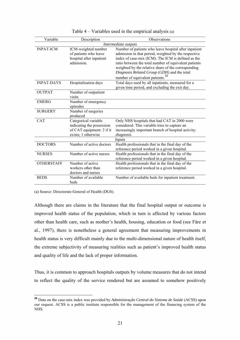
Table 4 – Variables used in the empirical analysis (a) Variable Description Observations

Intermediate outputs INPAT-ICM ICM-weighted number

of patients who leave hospital after inpatient admission.

Number of patients who leave hospital after inpatient admission in that period, weighted by the respective index of case-mix (ICM). The ICM is defined as the ratio between the total number of equivalent patients weighted by the relative share of the corresponding Diagnosis Related Group (GDH) and the total number of equivalent patients.28

INPAT-DAYS Hospitalisation days Total days used by all inpatients, measured for a given time period, and excluding the exit day.

OUTPAT Number of outpatient visits

EMERG Number of emergency episodes

SURGERY Number of surgeries produced

CAT Categorical variable indicating the possession of CAT equipment: 2 if it exists; 1 otherwise

Only NHS hospitals that had CAT in 2000 were considered. This variable tries to capture an increasingly important branch of hospital activity: diagnosis. Inputs

DOCTORS Number of active doctors Health professionals that in the final day of the reference period worked in a given hospital.

NURSES Number of active nurses Health professionals that in the final day of the reference period worked in a given hospital.

OTHERSTAFF Number of active workers other than doctors and nurses

Health professionals that in the final day of the reference period worked in a given hospital.

BEDS Number of available beds

Number of available beds for inpatient treatment.

(a) Source: Directorate-General of Health (DGS).

Although there are claims in the literature that the final hospital output or outcome is

improved health status of the population, which in turn is affected by various factors

other than health care, such as mother’s health, housing, education or food (see Färe et

al., 1997), there is nonetheless a general agreement that measuring improvements in

health status is very difficult mainly due to the multi-dimensional nature of health itself,

the extreme subjectivity of measuring realities such as patient’s improved health status

and quality of life and the lack of proper information.

Thus, it is common to approach hospitals outputs by volume measures that do not intend

to reflect the quality of the service rendered but are assumed to somehow positively

28 Data on the case-mix index was provided by Administração Central do Sistema de Saúde (ACSS) upon our request. ACSS is a public institute responsible for the management of the financing system of the NHS.

22

influence the health status of the population (Breyer, 1987).29 In this context, we

measure the number of hospitalised treated patients weighted by the respective index of

case-mix (INPAT-ICM),30 the total number of inpatient days (INPAT-DAYS), of

outpatient visits (OUTPAT), of emergency episodes (EMERG-TOT) and of surgeries

produced (SURGERY). We also consider a categorical variable indicating if a given

hospital has or has not CAT equipment since 2000 (CAT).

Table 5 summarises the descriptive statistics of our data set, where we observe the

significant positive relative change of both the number of outpatient visits and of

surgeries between 2000 and 2005. By contrast, there was a slight decrease in the

average number of available beds and in hospitalisation days for the same period.

29 See also Grosskopf and Valdmanis (1987). 30 To take into account the hospital case-mix, we weighted the number of treated patients by the corresponding index of case-mix (ICM) that is annually estimated by Instituto de Gestão Informática e Financeira da Saúde (IGIF) – variable INPAT-ICM.

23

Table 5 – Descriptive statistics of input and output variables Indicators 2000 2001 2002 2003 2004 2005

Beds Mean 296 313 283 282 281 283 Min. 28 13 17 8 22 18 Max. 1628 1628 1525 1530 1548 1505

Doctors Mean 189 204 192 185 185 189 Min. 8 7 7 8 8 8 Max. 1401 1401 1146 1090 1081 1148

Nurses Mean 313 333 319 323 332 342 Min. 24 25 25 27 27 32 Max. 1535 1542 1616 1559 1692 1727

Other Health Staff Mean 481 506 484 508 495 504 Min. 56 56 58 54 73 74

Inpu

ts

Max. 2143 2293 2165 4185 2401 2481 Inpatient Days

Mean 81745 85531 78293 78174 78176 79552 Min. 2912 2722 3804 1405 3145 2818 Max. 456801 456801 433207 441944 443051 437080

Outpatient Visits Mean 77350 85719 84206 90913 97424 102819 Min. 5554 8544 5259 8271 9146 9941 Max. 370046 394482 414475 444505 467734 495145

Emergencies Mean 81272 86148 81540 86243 79953 81802 Min. 4196 4346 707 3991 2462 781 Max. 225597 230609 225727 249420 233600 235111

Emergencies: treatment in the same hospital

Mean 6757 7823 7078 7247 7221 7152 Min. 24 276 174 143 215 195 Max. 28369 28517 28524 27374 25214 25161

Emergencies: transfer to another hospital

Mean 2358 2557 2670 2608 2530 2475 Min. 8 14 9 8 10 12 Max. 11419 11419 11277 9154 7586 6739

Inpatients weighted by ICM Mean 10887 11955 11395 11629 11848 12128 Min. 1325 1089 1202 492 544 1118 Max. 61722 62697 66404 66267 72745 69785

Surgeries Mean 4948 5681 5302 5727 5885 6045 Min. 314 382 233 233 15 426

Out

puts

Max. 35457 37428 33132 32444 28970 34199

24

4.2 – Model specifications

We use data on hospital services’ and resource quantities to construct an output distance

function, thus addressing the question: by how much can the (intermediate) output

quantities increase proportionally without changing input quantities? This approach is

consistent with the assumption that hospital managers behave as “resource-constrained

service maximisers” (see Lovell, 2002).

Valdmanis (1992), based on Nunamaker (1985), recommends that researchers should

specify within a DEA analysis different models from the dataset to evaluate whether the

ranking and efficiency of an individual DMU is variable-specific (or model-specific) or

whether the results are robust to changes in dataset specifications.31 Consequently, first

we defined a basic model and then we introduce changes that took the form of

alternative input/output definitions and/or the definition and selection of different

populations within our dataset.

In Table 6 we characterise the alternative models used in our analysis. In our basic

model (Model I) we only consider input and output variables for which we have

information for all the 68 hospitals for the 2000-2005 period (4 input and 5 output

variables), thus guaranteeing a balanced panel.

In order to test the effect of decreasing the number of input and output variables, we

specify Model II (2 input and 3 output variables).

As noted before, the classification of the hospitals may to some degree take account of

hospital’s case-mix and factors likely to affect the service rendered such as staffing

qualifications and medical technology used. To also take into account these differences

in our analysis, we specified Models III and IV where we selected within our dataset

only district hospitals and district level one hospitals. However, we added to the

analysis two more output variables because there is more information for this subgroup

in terms of outputs compared to the basic model (Model I). The cross-section sample

31 Another option is to compare the results of a DEA study with results from other efficiency evaluation methods (e.g. SFA) applied to the same dataset.

25

belonging to this group consists of 48 hospitals, 31 of which are district hospitals, and

17 are district hospitals level one.

The instability of the environmental context and of the regulatory regime of the NHS

hospitals spurred by the 2002 reform motivated the specification of Models V and VII,

where we individualize two sub-groups, SPA hospitals and SA/EPE hospitals,

respectively. In Model V and VII we use the same input and output variables specified

for Model I. Model VI and VIII only differ from the previous models in what concerns

the output measures used.

In order to test the homogeneity of our observations, we define two sub-groups of

hospitals based on the following criteria: those with CAT equipment since 2000 (34

hospitals), and those without CAT equipment since 2000 (34 hospitals), thus dividing

our initial sample into two equal parts.

26

Table 6 – Model Specifications Indicators Nº of

DMUs Description Models

Inputs # Outputs # I BEDS; DOCTORS;

NURSES; OTHERSTAFF

4 INPAT-DAYS; OUTPAT; EMERG-TOT; INPAT-ICM; SURGERY.

5

II BEDS; HEALTHSTAFF

2 OUTPAT; EMERG-TOT; INPAT-ICM. 3

68

These models include all observations.

III BEDS; DOCTORS; NURSES; OTHERSTAFF.

4 INPAT-DAYS; OUTPAT; EMERG-TOT; INPAT-ICM; SURGERY.

5

IV BEDS; DOCTORS; NURSES; OTHERSTAFF.

4 INPAT-DAYS; OUTPAT; EMERG-TOT; EMERG-NONTRANSF; EMERG-TRANSF; INPAT-ICM; SURGERY.

7

48

These models only consider district (DH) and district level-one (DH1) hospitals.

V BEDS; DOCTORS; NURSES; OTHERSTAFF.

4 INPAT-DAYS; OUTPAT; EMERG-TOT; INPAT-ICM; SURGERY.

5

VI BEDS; DOCTORS; NURSES; OTHERSTAFF.

4 INPAT-DAYS; OUTPAT; EMERG-TOT; EMERG-NONTRANSF; EMERG-TRANSF; INPAT-ICM; SURGERY.

7

34

These models only consider SPA hospitals.

VII BEDS; DOCTORS; NURSES; OTHERSTAFF.

4 INPAT-DAYS; OUTPAT; EMERG-TOT; INPAT-ICM; SURGERY.

5

VIII BEDS; DOCTORS; NURSES; OTHERSTAFF.

4 INPAT-DAYS; OUTPAT; EMERG-TOT; EMERG-NONTRANSF; EMERG-TRANSF; INPAT-ICM; SURGERY.

7

28

These models only consider SA/EPE hospitals.

IX BEDS; DOCTORS; NURSES; OTHERSTAFF

4 INPAT-DAYS; OUTPAT; EMERG-TOT; INPAT-ICM; SURGERY.

5

X BEDS; DOCTORS; NURSES; OTHERSTAFF.

4 INPAT-DAYS; OUTPAT; EMERG-TOT; EMERG-NONTRANSF; EMERG-TRANSF; INPAT-ICM; SURGERY.

7

34

These models only consider hospitals with CAT equipment in 2000.

XI BEDS; DOCTORS; NURSES; OTHERSTAFF.

4 INPAT-DAYS; OUTPAT; EMERG-TOT; INPAT-ICM; SURGERY.

5

XII BEDS; DOCTORS; NURSES; OTHERSTAFF.

4 INPAT-DAYS; OUTPAT; INPAT-ICM; SURGERY.

4

34

These models only consider hospitals without CAT equipment in 2000, regardless of having bought it afterwards.

XIII BEDS; DOCTORS; NURSES; OTHERSTAFF.

4 INPAT-DAYS; OUTPAT EMERG-TOT; INPAT-ICM; SURGERY.

5

XIV BEDS; DOCTORS; NURSES; OTHERSTAFF.

4 INPAT-DAYS; OUTPAT EMERG-TOT; EMERG-NONTRANSF; EMERG-TRANSF; INPAT-ICM; SURGERY.

7

62

These models only consider hospitals with emergency service information

27

Finally, we test two models (Models XIII and XIV) where only the NHS hospitals with

emergency service information were considered.32

4.3 – Results and discussion

We now turn to evaluate the productivity growth in the service provision of hospitals by

subjecting the data to a Malmquist index analysis.33 Additionally, in order to test if there

is any potential for efficiency and productivity improvements by the Portuguese NHS

hospitals and, if so, to quantify the corresponding magnitudes, the data was further

subjected to a yearly DEA analysis. Here, it is assumed that hospital managers attempt

to maximise the services that they provide and that such services can be approximated

by the indicators discussed in the preceding section. The DEA formulation that we use

in this study corresponds to the Charnes, Cooper and Rhodes (1978) formulation.34

Table 8 shows the evolution (annual means) of the Malmquist TFP index and of its

technological (T) and efficiency (E) components between 2000 and 2005 for Model I.

Table 8 – Mean Productivity Indices for Model I (2000-2005)

Efficiency Change (E)

Technical Change (T)

TFP /1

00/01 0.973 1.058 1.029 01/02 1.030 0.974 1.003 02/03 1.016 0.994 1.010 03/04 0.991 1.019 1.010 04/05 1.051 0.924 0.971 Mean 1.012 0.993 1.004

/1 TFP - Total Factor Productivity.

Preliminary estimates for our basic model (Model I) show that, on average, the NHS

hospital sector revealed positive but small productivity growth (TFP) levels between

2000 and 2004, whereas in 2005 there was a slight decrease in TFP. It is also possible to

32 Hospitals without emergency service information are the following ones: H. Santa Marta, H. Pulido Valente, H. Santa Cruz, H. Ortopédico de Outão, H. Joaquim Urbano and Instituto Oftalmológico Gama Pinto. 33 Measures of DEA distance functions and of Malmquist TFP index and its components (EC and TC) were estimated using the DEAP programme. The estimated DEA model imposes constant returns to scale, an option in line with the literature reviewed in Table 3. 34 For a detailed description of the DEA linear programming problem imposing constant returns to scale, see Grifell-Tatjé and Lovell (1995) and Coelli, Rao and Battese (1998).

28

conclude from Table 8 that the “efficiency change” component of TFP plays, on

average, a major role in productivity growth than the “technical change” component.

Furthermore, the TPF summary estimates for individual hospitals (annual means)

indicate that more than half of the NHS hospitals observed (42 out of 68) show either

positive or no relative change in TFP between 2000 and 2005, whereas the remaining

hospitals (26) show TFP decline (see Table A4 in the Appendix).

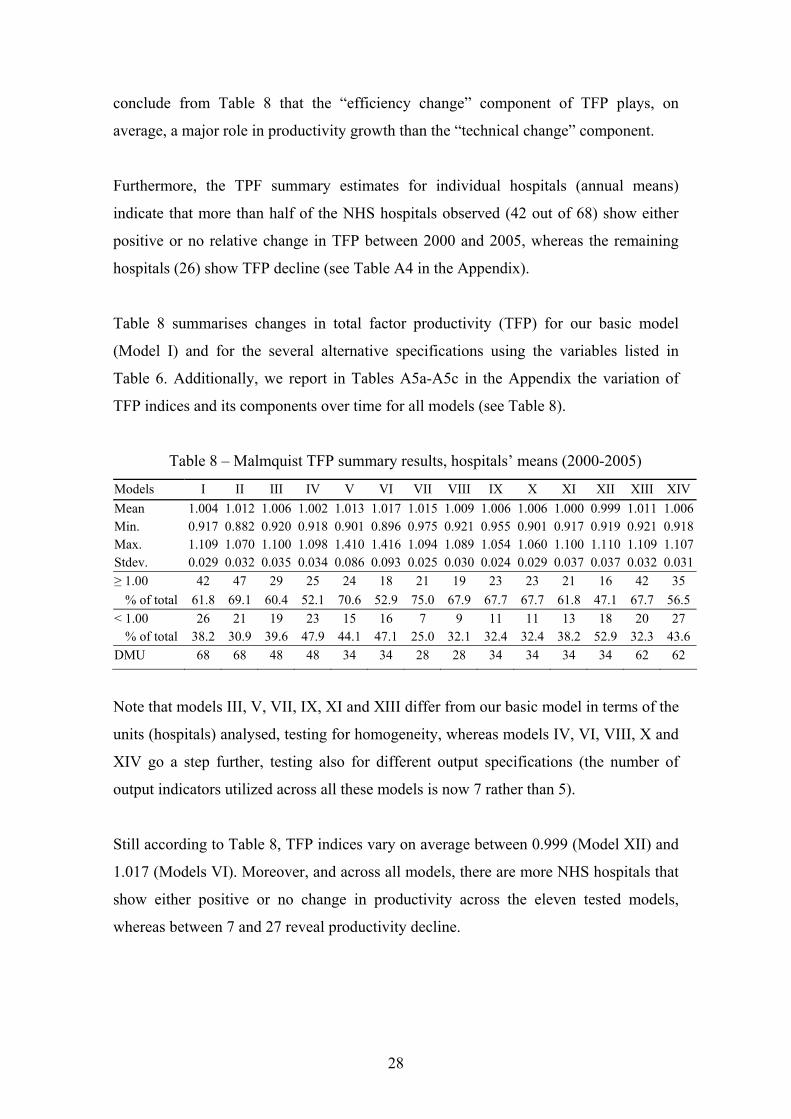
Table 8 summarises changes in total factor productivity (TFP) for our basic model

(Model I) and for the several alternative specifications using the variables listed in

Table 6. Additionally, we report in Tables A5a-A5c in the Appendix the variation of

TFP indices and its components over time for all models (see Table 8).

Table 8 – Malmquist TFP summary results, hospitals’ means (2000-2005)

Models I II III IV V VI VII VIII IX X XI XII XIII XIVMean 1.004 1.012 1.006 1.002 1.013 1.017 1.015 1.009 1.006 1.006 1.000 0.999 1.011 1.006Min. 0.917 0.882 0.920 0.918 0.901 0.896 0.975 0.921 0.955 0.901 0.917 0.919 0.921 0.918Max. 1.109 1.070 1.100 1.098 1.410 1.416 1.094 1.089 1.054 1.060 1.100 1.110 1.109 1.107Stdev. 0.029 0.032 0.035 0.034 0.086 0.093 0.025 0.030 0.024 0.029 0.037 0.037 0.032 0.031≥ 1.00 42 47 29 25 24 18 21 19 23 23 21 16 42 35

% of total 61.8 69.1 60.4 52.1 70.6 52.9 75.0 67.9 67.7 67.7 61.8 47.1 67.7 56.5 < 1.00 26 21 19 23 15 16 7 9 11 11 13 18 20 27

% of total 38.2 30.9 39.6 47.9 44.1 47.1 25.0 32.1 32.4 32.4 38.2 52.9 32.3 43.6 DMU 68 68 48 48 34 34 28 28 34 34 34 34 62 62

Note that models III, V, VII, IX, XI and XIII differ from our basic model in terms of the

units (hospitals) analysed, testing for homogeneity, whereas models IV, VI, VIII, X and

XIV go a step further, testing also for different output specifications (the number of

output indicators utilized across all these models is now 7 rather than 5).

Still according to Table 8, TFP indices vary on average between 0.999 (Model XII) and

1.017 (Models VI). Moreover, and across all models, there are more NHS hospitals that

show either positive or no change in productivity across the eleven tested models,

whereas between 7 and 27 reveal productivity decline.

29

The results of our sensitivity analysis highlight the specificity of Models XI and XII,

both with the lowest TFP averages observed (1.000 and 0.990, respectively), and

differing from each other only in terms of output specification.

The sub-group of 34 NHS hospitals analysed under these two models – hospitals not

having CAT equipment in the year 2000, regardless of having bought it afterwards –

registers the highest percentage of hospitals without emergency service information (62

percent). By contrast, only 24 percent (8 out of 34) of hospitals with CAT equipment in

the year 2000 didn’t have emergency service information.

If we compare Model I with those representing changes to it in terms of the units

included - Models III, V, VII, IX, XI and XIII –, from Table 8 it is possible to conclude

that:

- TFP behaves constantly through time across all these models until the period

2003-2004; from then on, both models V and IX depart from their previous

trend in what concerns TFP growth through time, but in opposite directions: as

for the first (second) model, TFP indices (average) decrease (increase) between

2003 and 2004, but then significantly increase (decrease) between 2004 and

2005;

- Model VII - which only considers SA/EPE hospitals - has the highest mean TFP

(1.015), but also the smallest number of DMU’s (28) within this context;

- Model V - which only considers SPA hospitals - has the second highest mean

TFP (1.013), but also the highest standard deviation, revealing more

heterogeneity within this sub-group of hospitals than, for instance, Models VII

and IX which consider SA/EPE hospitals and NHS hospitals with CAT

equipment in 2000, respectively;

- Model XIII - where only the NHS hospitals with emergency service information

were considered (62 hospitals) – registers a mean TFP slightly higher than that

reported for model I (1.011 and 1.004, respectively). It is interesting to note that

in this model the number of units with TFP mean values equal or greater than

unity equalizes that observed for model I (42 units). Therefore, the reduction in

the number of DMU’s from 68 to 62 improves TFP mean values because the six

30

DMU’s that are now missing were, in model I, within the group of those DMU’s

with TFP mean values inferior to unity (worse performers).

In general, the specification of models differing from the baseline specification only

differ in terms of the units considered, i.e., using the same set of input and output

variables but applying it to different sub-groups of hospitals, had by effect a general

increase of the TFP mean, with the exception of model XI.

The specification of a model (model II) to test the reduction of both input and output

indicators previously included in model I had by effect the increase of both the number

of units with TFP mean values equal or greater than unity (from 42 to 47 units) and of

the TPF mean (1.012, a value slightly higher than the reported for model I, 1.004).

Comparing TFP indices observed in our basic model with the several variations both in

terms of the units included and of the number of output indicators defined 35 - e.g.

Models IV, VI, VIII, X and XIV- it is possible to conclude from Table 8 that the mean

TFP does not significantly change, the exception being model VI - which refers to SPA

hospitals -, with a mean TFP slightly higher than that reported for model I (1,017 and

1,004, respectively). However, this increase was achieved at the expense of a wider

dispersion of the TFP mean values and of a reduction in the number of DMU’s observed

(from 68 to 34).

In general, increasing the number of (output) indicators translated into a reduction in the

number of hospitals with mean values of TFP equal or greater than unity.

It is possible to conclude that there are some differences in the computed Malmquist

indices across specifications. That circumstance motivated the examination of whether

the NHS hospitals change their efficiency scores within a particular model specification

across time.36

35 Increasing the number of output indicators from 5 to 7. 36 See Odeck (2005).

31

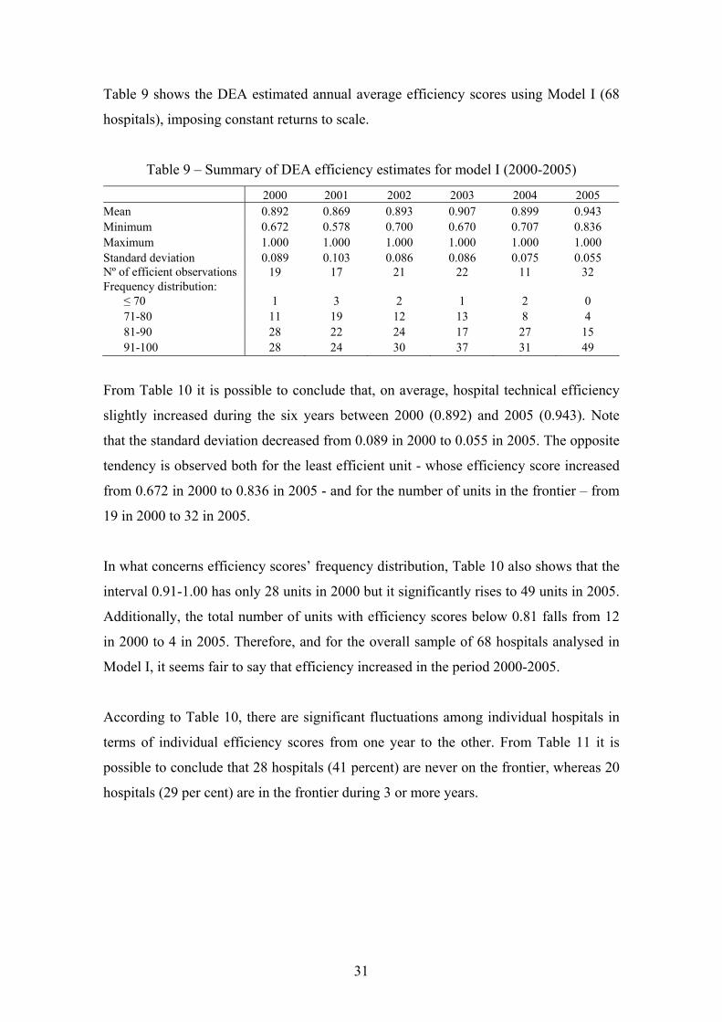
Table 9 shows the DEA estimated annual average efficiency scores using Model I (68

hospitals), imposing constant returns to scale.

Table 9 – Summary of DEA efficiency estimates for model I (2000-2005)

2000 2001 2002 2003 2004 2005 Mean 0.892 0.869 0.893 0.907 0.899 0.943 Minimum 0.672 0.578 0.700 0.670 0.707 0.836 Maximum 1.000 1.000 1.000 1.000 1.000 1.000 Standard deviation 0.089 0.103 0.086 0.086 0.075 0.055 Nº of efficient observations 19 17 21 22 11 32 Frequency distribution:

≤ 70 1 3 2 1 2 0 71-80 11 19 12 13 8 4 81-90 28 22 24 17 27 15 91-100 28 24 30 37 31 49

From Table 10 it is possible to conclude that, on average, hospital technical efficiency

slightly increased during the six years between 2000 (0.892) and 2005 (0.943). Note

that the standard deviation decreased from 0.089 in 2000 to 0.055 in 2005. The opposite

tendency is observed both for the least efficient unit - whose efficiency score increased

from 0.672 in 2000 to 0.836 in 2005 - and for the number of units in the frontier – from

19 in 2000 to 32 in 2005.

In what concerns efficiency scores’ frequency distribution, Table 10 also shows that the

interval 0.91-1.00 has only 28 units in 2000 but it significantly rises to 49 units in 2005.

Additionally, the total number of units with efficiency scores below 0.81 falls from 12

in 2000 to 4 in 2005. Therefore, and for the overall sample of 68 hospitals analysed in

Model I, it seems fair to say that efficiency increased in the period 2000-2005.

According to Table 10, there are significant fluctuations among individual hospitals in

terms of individual efficiency scores from one year to the other. From Table 11 it is

possible to conclude that 28 hospitals (41 percent) are never on the frontier, whereas 20

hospitals (29 per cent) are in the frontier during 3 or more years.

32

Table 10 – DEA-CRS estimates per hospital for model I (2000-2005)

Hospitals

2000

2001

2002

2003

2004

2005

n. times on

frontier H. Águeda 1,000 1,000 1,000 1,000 0,863 1,000 5 H. Infante D. Pedro / Aveiro 0,881 0,825 0,835 0,913 0,857 0,966 0 H. São Miguel / Oliveira de Azeméis 0,975 1,000 1,000 1,000 0,895 1,000 4 H. São João da Madeira 0,875 0,882 1,000 0,971 0,808 1,000 2 H. São Sebastião da Feira 1,000 1,000 1,000 1,000 1,000 1,000 6 H. José Luciano de Castro / Anadia 0,820 0,851 0,700 1,000 0,841 0,962 1 H. Dr. Francisco Zagalo / Ovar 0,855 0,920 0,918 0,915 0,872 1,000 1 H. Nossa Senhora da Ajuda / Espinho 1,000 1,000 1,000 1,000 1,000 1,000 6 H. Visconde de Salreu / Estarreja 0,847 0,804 1,000 0,942 0,903 1,000 2 H. São Marcos / Braga 0,872 0,884 0,943 0,948 0,886 0,935 0 H. Santa Maria Maior / Barcelos 0,795 0,833 0,886 0,875 0,811 1,000 1 H. São João de Deus / Famalicão 0,809 0,770 0,700 0,761 0,747 0,814 0 H. Senhora da Oliveira / Guimarães 1,000 1,000 1,000 1,000 0,970 1,000 5 H. São José / Fafe 1,000 0,852 0,833 0,882 0,842 0,972 1 H. Bragança 1,000 0,922 0,870 1,000 0,902 1,000 3 H. Mirandela 0,848 0,941 1,000 0,862 0,744 0,896 1 H. Macedo de Cavaleiros 1,000 0,968 1,000 1,000 1,000 1,000 5 H.C. Cova da Beira (H. Covilhã; H. Fundão) 0,921 0,797 0,820 0,780 0,886 0,861 0 H. Amato Lusitano / Castelo Branco 0,797 0,785 0,770 0,768 0,756 0,832 0 H. Universidade de Coimbra 0,868 0,874 0,900 0,880 0,903 0,940 0 H. Figueira da Foz 0,742 0,762 0,755 0,795 0,823 0,923 0 H. Arcebispo João Crisóstomo / Cantanhede 0,900 0,999 0,899 0,999 0,903 0,794 0 H. Espírito Santo / Évora 0,846 0,743 0,796 0,820 0,831 0,756 0 H. Faro 0,849 0,837 0,854 0,883 0,948 0,925 0 H. Sousa Martins / Guarda 0,903 0,879 0,874 0,971 0,836 1,000 1 H. Nossa Senhora da Assunção / Seia 0,907 1,000 1,000 1,000 1,000 1,000 5 H.C. Caldas da Rainha 1/ 0,886 0,578 0,813 0,808 0,894 0,844 0 H. Santo André / Leiria 0,977 0,893 0,942 1,000 0,906 1,000 2 H. Bernardino Lopes de Oliveira / Alcobaça 1,000 1,000 1,000 1,000 1,000 1,000 6 H. Pombal 1,000 1,000 1,000 1,000 1,000 1,000 6 H. São Pedro Gonçalves Telmo / Peniche 1,000 1,000 1,000 1,000 0,995 1,000 5 H. Prof. Dr. Fernando Fonseca 1,000 0,973 0,855 0,873 0,996 1,000 2 H. Curry Cabral 1,000 1,000 0,906 1,000 0,964 0,993 3 H. Egas Moniz 0,834 0,816 0,801 0,808 0,836 0,921 0 H. Pulido Valente 0,816 0,780 0,750 0,798 0,910 0,862 0 H. Santa Cruz 1,000 1,000 1,000 1,000 1,000 1,000 6 H. Santa Maria 0,985 0,934 0,886 0,844 0,940 0,842 0 H. Santa Marta 0,847 0,878 1,000 1,000 0,983 1,000 3 H. São Francisco Xavier 0,916 0,879 0,889 0,902 0,959 0,936 0 Oftalmologic Institute Gama Pinto 1,000 1,000 1,000 1,000 1,000 1,000 6 Maternity D.Estefânia 0,815 0,723 0,836 0,812 0,991 0,939 0 Maternity Alfredo da Costa 0,855 0,712 0,788 0,823 0,948 1,000 1 H. Reinaldo dos Santos / V. F. Xira 1,000 0,858 0,933 0,918 1,000 1,000 3 H. Dr. José Maria Grande / Portalegre 0,878 0,807 0,906 0,957 0,821 1,000 1 H. Santa Luzia / Elvas 0,774 0,797 0,790 0,854 0,824 0,869 0 H.C. Vila Nova de Gaia 1/ 0,833 0,828 0,828 0,769 0,924 0,873 0 H. Joaquim Urbano 1,000 1,000 1,000 1,000 0,766 1,000 5 H. Maria Pia 0,706 0,640 0,769 0,670 0,796 0,910 0 H. Santo António 0,889 0,875 1,000 0,857 0,979 0,988 1

33

Table 10 (cont.)

Hospitals

2000

2001

2002

2003

2004

2005

n. times on frontier

H. São João 0,850 0,792 0,849 0,855 0,887 0,867 0 Maternity Júlio Dinis 0,672 0,857 0,916 0,749 0,763 0,907 0 H.C. Padre Américo / Vale de Sousa 0,913 0,768 0,830 0,887 0,943 1,000 1 H. Nossa Senhora da Conceição / Valongo 1,000 1,000 1,000 1,000 1,000 1,000 6 H. Pedro Hispano 37 0,956 0,907 1,000 0,976 0,973 1,000 2 H. Conde de São Bento / Santo Tirso 0,847 0,835 0,946 0,953 0,928 1,000 1 H. São Gonçalo / Amarante 0,744 0,714 0,958 1,000 0,893 1,000 2 H. Santarém 0,806 0,773 0,839 0,875 0,937 0,935 0 H. Ortopédico Santiago do Outão 0,855 0,899 0,954 0,914 0,938 0,954 0 H de S. Bernardo / Setúbal 0,838 0,842 0,846 0,785 0,975 0,851 0 H. Garcia de Orta / Almada 0,866 0,804 0,857 0,824 0,934 1,000 1 H. Nossa Senhora do Rosário / Barreiro 0,735 0,703 0,754 0,755 0,860 0,836 0 H. Litoral Alentejano / Santiago do Cacém38 1,000 1,000 1,000 1,000 0,868 0,926 4 H. Montijo 0,720 0,768 0,716 0,779 0,706 0,767 0 H. Chaves 0,770 0,728 0,762 0,807 0,784 0,781 0 H. Lamego 0,917 0,777 0,897 0,948 0,707 1,000 1 H. São Teotónio / Viseu 0,842 0,830 0,849 0,946 0,890 0,987 0 H. Cândido de Figueiredo / Tondela 1,000 1,000 0,774 1,000 0,875 0,863 3 H.C. Coimbra 0,983 1,000 0,947 0,980 1,000 0,899 2 Summary statistics Mean 0,892 0,869 0,893 0,907 0,899 0,943 Minimum 0,672 0,578 0,700 0,670 0,706 0,756 Maximum 1,000 1,000 1,000 1,000 1,000 1,000 Standard deviation 0,091 0,105 0,092 0,090 0,082 0,071 Notes: H.- Hospital; H.C.- Hospital Center.

Looking at the number of hospitals in the production possibility frontier maintaining

their relative positions, only 7 hospitals (10 per cent) stay on the frontier during all the

period of observation (6 years), of which 5 are SPA hospitals 2 are EPE hospitals. Of

these 7 efficient hospitals, only 2 are Central (H. Santa Cruz, I.O. Gama Pinto), and the

remaining 5 are District (H. São Sebastião da Feira, H. Nossa Senhora da Ajuda /

Espinho, H. Bernardino Lopes de Oliveira / Alcobaça, H. Pombal, H. Nossa Senhora da

Conceição / Valongo). Additionally, the mean efficiency scores of 15 per cent of the

hospitals have fallen between 2000 and 2005, eventually indicating some difficulties in

terms of productive efficiency over time, and signalling a theoretical corresponding

margin of manoeuvre for improvements.

37 Matosinhos’ Local Health Unit (Unidade Local de Saúde). 38 Previously, Hospital Conde do Bracial.

34

Table 10 also shows that the efficiency four hospitals (H. Águeda, H. Senhora da

Oliveira / Guimarães, H. São Pedro Gonçalves Telmo / Peniche, H. Joaquim Urbano)

are consistently on the frontier over time. Finally, it is also possible to conclude that

mean efficiency scores have been improving since 2000, for the entire set of 68

hospitals (Model I) of the NHS.

5 – CONCLUSION

In this study we used a data set of contiguous panel data comprising a sample of 68

Portuguese public hospitals in the years 2000-2005. Estimates for our baseline model

show that, on average, the NHS hospital sector revealed positive but small productivity

growth (Total Factor Productivity – TFP) levels between 2000 and 2004, whereas in

2005 there was a slight decrease in TFP.

Taking into account our basic model and several alternative specifications it is possible

to see that the mean TFP indices vary between 0.917 and 1.109, implying that there are

some differences in the computed Malmquist indices across specifications. That

circumstance motivated the estimation of annual DEA efficiency scores for each model

specification. In fact, there are significant fluctuations among NHS hospitals in terms of

individual efficiency scores from one year to the other. Looking at the number of

hospitals located in the production possibility frontier that maintain their relative

positions, 27 out of 68 units appear on the frontier more than once and only 7 hospitals

(10 percent) stay on the frontier in all years of the analysis.

Additionally, the mean efficiency scores of 15 per cent of the hospitals have fallen

between 2000 and 2005, eventually indicating some difficulties in terms of productive

efficiency over time, and signalling a theoretical corresponding margin of manoeuvre

for improvements. Indeed, the analyses suggests that there is scope for developing

performance indicators at hospital level, and also using panel data, in order to assess

how hospitals can move towards the efficiency frontier. Finally, and in terms of future

work, a two-step approach could also be used to study the possible determinants of

inefficiencies observed in our sample of NHS hospitals.

35

REFERENCES

Afonso, A. and St. Aubyn, M. (2005). “Non-parametric Approaches to Education and Health Efficiency in OECD Countries”, Journal of Applied Economics, 8 (2), 227-246. Afonso, A. and St. Aubyn, M. (2006). “Cross-country Efficiency of Secondary Education Provision: a Semi-parametric Analysis with Non-discretionary Inputs”, Economic Modelling, 23 (3), 476-491. Afonso, A. and Fernandes, S. (2006). “Measuring local government spending efficiency: Evidence for the Lisbon Region”, Regional Studies, 40 (1), 39-53. Afonso, A.; Schuknecht, L. and Tanzi, V. (2005). “Public Sector Efficiency: an International Comparison,” Public Choice, 123 (3-4), 321-347. Aigner, D. and Chu, S. (1968). “On estimating the Industry Production Frontiers”, American Economic Review, 58, 826-839. Aigner, D; Lovell, C. and Schmidt, P. (1977). “Formulation and estimation of Stochastic Frontier Production Function Models”, Journal of Econometric, 6, 21-37. Balk, B. (1998), Industrial Price, Quantity and Productivity Indices, The Micro-economic Theory and an Application, Kluwer Academic Publishers. Bentes, M; Dias, C.; Sakellarides, C. (2004). Health care systems in transition: Portugal, Copenhagen, WHO Regional Office for Europe on behalf of the European Observatory on Health Systems and Policies. Breyer, F. (1987). “The Specification of a Hospital Cost Function – A Comment on the Recent Literature”, Journal of Health Economics, 6, 147-157. Burgess, J. and Wilson, P. (1995), “Decomposing hospital productivity changes, 1985-1988: A non-parametric Malmquist approach, Journal of Productivity Analysis, 6, 342-363. Caves, D. , Christensen, L. and Diewert, W. (1982).”The Economic Theory of Index Numbers and the Measurment of Input, Output and Productivity”, Econometrica, 50, 1393-1414. Charnes, A.; Cooper, W. and Rhodes, E. (1978). “Measuring the Efficiency of Decision Making Units”, European Journal of Operational Research, 2 (6), 429-444. Chirikos, T. and Sear, A. (2000) "Measuring hospital efficiency: A comparison of two approaches", Health Services Research, 34 (6), 1389-408. Coelli, T.; Rao, D. and Battese, G. (1998). An Introduction to Efficiency and Productivity Analysis, Sixth Printing (2002), Massachusetts, Kluwer Academic Publishers.

36

Coelli, T. (2002). “A Comparison of Alternative Productivity Growth Measures: With Application to Electricity Generation”, in: Fox, Kevin J. (ed.), Efficiency in the Public Sector, Kluwer, 169-200. Dixon, A. and Mossialos, E. (2000). “Has the Portuguese NHS achieved its objectives of equity and efficiency?”, International Social Security Review, 53(4), 49-78. Docteur, E. and H. Oxley (2003). Health-Care Systems: Lessons from the Reform Experience, OECD Health Working Papers, No. 9, OECD Publishing. Färe, R.; Grosskopf, S., Lindgren, B. and Poullier, J. P. (1997). “Productivity growth in health cared delivery”, Medical Care, 35, 354-366. Färe, R.; Grosskopf, S., Lindgren, B. and Roos, P. (1994). “Productivity developments in Swedish hospitals: A Malmquist output index approach”, in: Charnes, A.; Cooper, W., Lewin, A. and Seiford L. (eds.), Data Envelopment Analysis: Theory, Methodology and Applications, Boston, Kluwer, 253-272. Farrell, M. (1957). “The Measurement of Productive Efficiency”, Journal of the Royal Statistical Society Series A (General), 120 (3), 253-281. Grifell-Tatjé, E. and Lovell, C. (1995). “A Note on the Malmquist Productivity Index”, Economics Letters, 47, 169-75. Grosskopf, S. (1993). “Efficiency and Productivity”, in Fried H. O., Lovell, C. A. K. and Schmidt, S. S. (eds.), The Measurement of Productive Efficiency: Techniques and Applications, New York, Oxford University Press, 160-194. Hollingsworth, B. (2003), “Non-parametric and Parametric Applications Measuring Efficiency in Health Care”, Health Care Management Science, 6, 203-218. Hollingsworth, B.; Dawson, P. and Maniadakis, N. (1999). “Efficiency measurement of health care: A review of non-parametric methods and applications”, Health Care Management Science, 2, 161–172. Jacobs, R.; Smith, P. and Street, A. (2006). Measuring Efficiency in Health Care, Cambridge, Cambridge University Press. Lima, E. and Whynes, D. K. (2003). Finance and Performance of Portuguese Hospitals, Working Paper nº 20, Núcleo de Investigação em Microeconomia Aplicada, Braga, Universidade do Minho. Linna, M. (1998). “Measuring hospital cost efficiency with panel data models”, Health Economics, 7, 415-427. Linna, M. (2000). “Health Care Financing Reform and the Productivity Change in Finnish Hospitals”, Jpurnal of Health Care Financing, 26(3), 83-100.

37

Lovell C. (2000). “Measuring Efficiency in the Public Sector”, in: Blank, Jos L. T. (ed.), Public Provision and Performance, Amsterdam, North-Holland, 23-53. Lovell, C. (2002). “Performance Assessment in the Public Sector”, in: Fox, Kevin J. (ed.), Efficiency in the Public Sector, Kluwer Academic Publishers, 11-35. Lovell, C. (2006). “Malmquist Productivity Index – Government Funded Education Services”, in: Avkiran, Necmi K. (ed.), Productivity Analysis in the Service Sector with Data Envelopment Analysis, third edition, publisher Necmi K. Avkiran, University of Queensland, Brisbane-Australia, 149-161. Malmquist, S. (1953). “Index numbers and indifference surfaces”, Trabajos de Estatistica, 4, 209-242. Maniadakis N.; Hollingsworth, B. and Thanassoulis, E. (1999). “The Impact of the Internal Market on Hospital Efficiency, Productivity and Service Quality”, Journal of Health Care Management Science , 2(2), 75-85. Maniadakis, N and Thanassoulis, E. (2000). “Changes in Productivity of a Sample of Scottish Hospitals: A Cost Index Approach”, Applied Economics, 32, 1575-1589. McCallion, G.; Glass, J. , Jackson, R., Kerr, C. and McKillop, D. (2000). “Investigating productivity change and hospital size: A non-parametric approach”, Applied Economics, 32, 161–174. McKee, M. and Healy, J. (eds.) (2002). Hospitals in a changing Europe, European Observatory on Health Care Systems Series, Buckingham, Open University Press. Meeusen, W. and van den Broeck, J. (1977). “Efficiency estimation from Cobb-Douglas Production Functions with Composed Error”, International Economic Review, 18, 435-444. Nishimizu, M. and Page, J. (1982). “Total Factor Productivity Growth, Technical Progress and Technical Efficiency Change: Dimensions of Productivity Change in Yugoslavia, 1965-78”, Economic Journal, 92, 920-936. Nunamaker, T. (1985). “Using Data Envelopment Analysis to Measure the Efficiency of Non-Profit Organizations: A Critical Evaluation”, Managerial and Decision Economics, 6(1), 50-58. Odeck, J. (2005). “Evaluating Target Achievements in the Public Sector: An Application of a Rare Non-Parametric DEA and Malmquist Indices” Journal of Applied Economics, 8(1), 171-190. OECD (2001). Measuring Productivity: Measurement of Aggregate and Industry Level Productivity Growth, OECD, Paris. Available in 26.11.2006 in the following URL: http://www.oecd.org/dataoecd/59/29/2352458.pdf OECD (2004). OECD Health Data 2004. OECD, Paris.

38

OECD (2005). OECD Health Data 2005. OECD, Paris. Oliveira, M. (2002). “Will hospital Management Reform in Portugal Work?”, Euro Observer. Newsletter of the European Observatory on Health Care Systems, 4, 3-4. Oliveira, M. and Pinto, C. (2005). “Health care reform in Portugal: an evaluation of the NHS experience”, Health Economics, 14, 203-220. Portuguese Observatory on Health Care Systems (2001). Conhecer os Caminhos da Saúde, Spring Report, ENSP: Lisbon. Quintela, I.; Carvalho, A. and Tranquada, S. (2006). “The Portuguese Experience: Estimation of the output of hospitals according to different methodologies”, Paper presented for the joint OECD/ONS/Government of Norway workshop, Measurement of non-market output in education and health, London, October 3-5. Seiford, L. and Thrall, R. (1990). “Recent Developments in DEA: The Mathematical Programming Approach to Frontier Analysis”, Journal of Econometrics, 46, 7-38. Shepard, R. W. (1970). Theory of Cost and Production Functions, Princeton, Princeton University Press. Solà, M. and Prior, D. (2001), “Measuring productivity and Quality Changes using Data Envelopment Analysis: An Application to Catalan Hospitals”, Financial Accountability and Management, 17(3), 219-245. Sommersguter-Reichmann, M. (2000). “The impact of the Austrian hospital financing reform on hospital productivity: empirical evidence on efficiency and technology changes using a non-parametric input-based Malmquist approach”, Health Care Management Science, 3, 309-321. Valdmanis, V. (1992). “Sensitivity analysis for DEA models: An empirical example using public vs. NFP hospitals”, Journal of Public Economics, 48, 185–205. Zere, E. (2000), Hospital Efficiency in Sub-Saharan Africa Evidence from South Africa, Working Paper 187 (June), World Institute for Development Economics Research: The United Nations University. Zere E.; McIntyre D. and Addison T. (2001). “Technical efficiency and productivity of public sector hospitals in three South African provinces”, South African Journal of Economics, 69(2), 336-358.