Assessing heterogeneity in meta-analysis: Q statistic or I2 index?

University of ConnecticutDigitalCommons@UConn

CHIP Documents Center for Health, Intervention, and Prevention(CHIP)

6-1-2006

Assessing heterogeneity in meta-analysis: Q statisticor I2 index?Tania Huedo-MedinaUniversity of Connecticut, [email protected]

Julio Sanchez-MecaUniversity of Murcia, Spane

Fulgencio Marin-MartinezUniversity of Murcia, Spain

Juan BotellaAutonoma University of Madrid, Spain

Follow this and additional works at: http://digitalcommons.uconn.edu/chip_docs

Part of the Psychology Commons

Recommended CitationHuedo-Medina, Tania; Sanchez-Meca, Julio; Marin-Martinez, Fulgencio; and Botella, Juan, "Assessing heterogeneity in meta-analysis:Q statistic or I2 index?" (2006). CHIP Documents. 19.http://digitalcommons.uconn.edu/chip_docs/19

http://lib.uconn.edu/?utm_source=digitalcommons.uconn.edu%2Fchip_docs%2F19&utm_medium=PDF&utm_campaign=PDFCoverPages

http://lib.uconn.edu/?utm_source=digitalcommons.uconn.edu%2Fchip_docs%2F19&utm_medium=PDF&utm_campaign=PDFCoverPages

http://digitalcommons.uconn.edu?utm_source=digitalcommons.uconn.edu%2Fchip_docs%2F19&utm_medium=PDF&utm_campaign=PDFCoverPages

http://digitalcommons.uconn.edu/chip_docs?utm_source=digitalcommons.uconn.edu%2Fchip_docs%2F19&utm_medium=PDF&utm_campaign=PDFCoverPages

http://digitalcommons.uconn.edu/chip?utm_source=digitalcommons.uconn.edu%2Fchip_docs%2F19&utm_medium=PDF&utm_campaign=PDFCoverPages

http://digitalcommons.uconn.edu/chip?utm_source=digitalcommons.uconn.edu%2Fchip_docs%2F19&utm_medium=PDF&utm_campaign=PDFCoverPages

http://digitalcommons.uconn.edu/chip_docs?utm_source=digitalcommons.uconn.edu%2Fchip_docs%2F19&utm_medium=PDF&utm_campaign=PDFCoverPages

http://network.bepress.com/hgg/discipline/404?utm_source=digitalcommons.uconn.edu%2Fchip_docs%2F19&utm_medium=PDF&utm_campaign=PDFCoverPages

http://digitalcommons.uconn.edu/chip_docs/19?utm_source=digitalcommons.uconn.edu%2Fchip_docs%2F19&utm_medium=PDF&utm_campaign=PDFCoverPages

ASSESSING HETEROGENEITY IN META-ANALYSIS:

Q STATISTIC OR I2 INDEX?

Tania B. Huedo-Medina,1 Julio Sánchez-Meca,1 Fulgencio Marín-Martínez,1

and Juan Botella2

Running head: Assessing heterogeneity in meta-analysis

2006

1 University of Murcia, Spain2 Autónoma University of Madrid, Spain

Address for correspondence:

Tania B. Huedo-Medina

Dept. of Basic Psychology & Methodology, Faculty of Psychology, Espinardo Campus,

Murcia, Spain

Phone: + 34 968 364279

Fax: + 34 968 364115

E-mail: [email protected]

* This work has been supported by Plan Nacional de Investigación Científica,Desarrollo e Innovación Tecnológica 2004-07 from the Ministerio de Educación yCiencia and by funds from the Fondo Europeo de Desarrollo Regional, FEDER(Proyect Number: SEJ2004-07278/PSIC).

Assessing heterogeneity in meta-analysis 2



Abstract

In meta-analysis, the usual way of assessing whether a set of single studies are

homogeneous is by means of the Q test. However, the Q test only informs us about the

presence versus the absence of heterogeneity, but it does not report on the extent of such

heterogeneity. Recently, the I2 index has been proposed to quantify the degree of

heterogeneity in a meta-analysis. In this paper, the performances of the Q test and the

confidence interval around the I2 index are compared by means of a Monte Carlo

simulation. The results show the utility of the I2 index as a complement to the Q test,

although it has the same problems of power with a small number of studies.

KEY WORDS: Meta-analysis, effect size, heterogeneity, I2 index, Monte Carlo method.




In the last 25 years meta-analysis has been widely accepted in the social and health

sciences as a very useful research methodology to quantitatively integrate the results of

a collection of single studies on a given topic. In a meta-analysis the result of every

study is quantified by means of an effect-size index (e.g., standardized mean difference,

correlation coefficient, odds ratio, etc.) that can be applied to all studies, enabling us to

give the study results in the same metric (Cooper, 1998; Cooper & Hedges, 1994;

Egger, Smith, & Altman, 2001; Glass, McGaw, & Smith, 1981; Hedges & Olkin, 1985;

Hunter & Schmidt, 2004; Rosenthal, 1991; Sutton, Abrams, Jones, Sheldon, & Song,

2000; Whitehead, 2002).

Typically, meta-analysis has three main goals: (a) to test whether the studies

results are homogeneous, (b) to obtain a global index about the effect magnitude of the

studied relation, joined to a confidence interval and its statistical significance, and (c) if

there is heterogeneity among studies, to identify possible variables or characteristics

moderating the results obtained. Here, we focus on how to assess the heterogeneity

among the results from a collection of studies. Basically, there can be two sources of

variability that explain the heterogeneity in a set of studies in a meta-analysis. One of

them is the variability due to sampling error, also named within-study variability. The

sampling error variability is always present in a meta-analysis, because every single

study uses different samples. The other source of heterogeneity is the between-studies

variability, which can appear in a meta-analysis when there is true heterogeneity among

the population effect sizes estimated by the individual studies. The between-studies

variability is due to the influence of an indeterminate number of characteristics that vary

among the studies, such as those related to the characteristics of the samples, variations

in the treatment, in the design quality, and so on (Brockwell & Gordon, 2001; Erez,

Bloom, & Wells, 1996; Field, 2003; Hunter & Schmidt, 2000; National Research

Council, 1992).

To assess the heterogeneity in meta-analysis is a crucial issue because the

presence versus the absence of true heterogeneity (between-studies variability) can

affect the statistical model that the meta-analyst decides to apply to the meta-analytic


database. So, when the studies’ results only differ by the sampling error (homogeneous

case) a fixed-effects model can be applied to obtain an average effect size. By contrast,

if the study results differ by more than the sampling error (heterogeneous case), then the

meta-analyst can assume a random-effects model, in order to take into account both

within- and between-studies variability, or can decide to search for moderator variables

from a fixed-effects model (Field, 2001, 2003; Hedges, 1994; Hedges & Olkin, 1985;

Hedges & Vevea, 1998; Overton, 1998; Raudenbush, 1994).

The usual way of assessing whether there is true heterogeneity in a meta-

analysis has been to use the Q test, a statistical test defined by Cochran (1954). The Q

test is computed by summing the squared deviations of each study’s effect estimate

from the overall effect estimate, weighting the contribution of each study by its inverse

variance. Under the hypothesis of homogeneity among the effect sizes, the Q statistic

follows a chi-square distribution with k – 1 degrees of freedom, k being the number of

studies. Not rejecting the homogeneity hypothesis usually leads the meta-analyst to

adopt a fixed-effects model because it is assumed that the estimated effect sizes only

differ by sampling error. In contrast, rejecting the homogeneity assumption can lead to

applying a random-effects model that includes both within- and between-studies

variability. A shortcoming of the Q statistic is that it has poor power to detect true

heterogeneity among studies when the meta-analysis includes a small number of studies

and excessive power to detect negligible variability with a high number of studies

(Alexander, Scozzaro, & Borodkin, 1989; Cornwell, 1993; Cornwell & Ladd, 1993;

Hardy & Thompson, 1998; Harwell, 1997; Osburn, Callender, Greener, & Ashworth,

1983; Paul & Donner, 1992; Sackett, Harris, & Orr, 1986; Sagie & Koslowsky, 1993;

Sánchez-Meca & Marín-Martínez, 1997; Spector & Levine, 1987). Thus, a non-

significant result for the Q test with a small number of studies can lead a reviewer to

erroneously assume a fixed-effects model when there is true heterogeneity among the

studies; and vice versa. On the other hand, the Q statistic does not inform us of the

extent of true heterogeneity, only of its statistical significance.1

1 It is important to note that the low statistical power of the Q test for small number of studies haspromoted the undesirable practice among some meta-analysts of ignoring the results of Q when it is notstatistically significant, and searching for moderator variables. On the other hand, the meta-analyst can apriori adopt a statistical model (fixed- or random-effects model) on conceptual grounds. For example, ifthe meta-analyst wishes to generalize the meta-analytic results to a population of studies with similarcharacteristics than those of represented in the meta-analysis, a fixed-effects model can be selected. If, on


Another strategy for quantifying the true heterogeneity in a meta-analysis

consists of estimating the between-studies variance, τ2. Assuming a random-effects

model, the between-studies variance reflects how much the true population effect sizes

estimated in the single studies of a meta-analysis differ. As the τ2 depends on the

particular effect metric used in a meta-analysis, it is not possible to compare the τ2

values estimated from meta-analyses that have used different effect-size indices (e.g.,

standardized mean differences, correlation coefficients, odds ratios, etc.).

In order to overcome the shortcomings of the Q test and the τ2, Higgins and

Thompson (2002; see also Higgins, Thompson, Deeks, & Altman, 2003) have proposed

three indices for assessing heterogeneity in a meta-analysis: the H2, R2, and I2 indices.

As they are inter-related, here we focus on the I2 index, because of its easy

interpretation. The I2 index measures the extent of true heterogeneity dividing the

difference between the result of the Q test and its degrees of freedom (k – 1) by the Q

value itself, and multiplied by 100. So, the I2 index is similar to an intraclass correlation

in cluster sampling (Higgins & Thompson, 2002). The I2 index can be interpreted as the

percentage of the total variability in a set of effect sizes due to true heterogeneity, that

is, to between-studies variability. For example, a meta-analysis with I2 = 0 means that

all variability in effect size estimates is due to sampling error within studies. On the

other hand, a meta-analysis with I2 = 50 means that half of the total variability among

effect sizes is caused not by sampling error, but by true heterogeneity between studies.

Higgins and Thompson (2002) proposed a tentative classification of I2 values with the

purpose of helping to interpret its magnitude. Thus, percentages of around 25% (I2 =

25), 50% (I2 = 50), and 75% (I2 = 75) would mean low, medium, and high

heterogeneity, respectively. The I2 index and the between-studies variance, τ2, are

directly related: the higher the τ2, the higher the I2 index. However, following Higgins

and Thompson (2002), an advantage of the I2 index in respect to τ2 is that I2 indices

obtained from meta-analyses with different numbers of studies and different effect

metrics are directly comparable.

the contrary, the meta-analytic results have to be generalized to a wider population of studies, a random-effects model should be the best option (Field, 2001; Hedges & Vevea, 1998).


Together with this descriptive interpretation of the I2 index, Higgins and

Thompson (2002) have derived a confidence interval for it that might be used in the

same way as the Q test is used to assess heterogeneity in meta-analysis. Thus, if the

confidence interval around I2 contains the 0% value, then the meta-analyst can hold the

homogeneity hypothesis. If, on the contrary, the confidence interval does not include the

0% value, then there is evidence for the existence of true heterogeneity. Using the I2

index and its confidence interval is similar to applying the Q test. Because the I2 index

assesses not only heterogeneity in meta-analysis, but also the extent of that

heterogeneity, it should be a more advisable procedure than the Q test in assessing

whether or not there is true heterogeneity among the studies in a meta-analysis.

However, the performance of the confidence interval around I2 has not yet been studied

in terms of the control of Type I error rate and statistical power.

The purpose of this paper is to compare, by a Monte Carlo simulation, the

performance of the Q test and the confidence interval around the I2 index, in terms of

their control of Type I error rate and statistical power. Different effect-size indices were

used and both the extent of true heterogeneity and the number of studies were varied.

Thus, it is possible to test whether the confidence interval for I2 overcomes the

shortcomings of the Q test.

Effect-size indices

For each individual study, we assume two underlying populations representing the

experimental versus control groups on a continuous outcome. Let µE and µC be the

experimental and control population means, and σE and σC the population standard

deviations, respectively. By including a control condition in the typical design we

restrict the applicability of our results to research fields in which such designs make

sense (e.g., treatment outcome evaluation in behavioral sciences, education, medicine,

etc.). Under the assumptions of normal distributions and homoscedasticity, the usual

parametric effect-size index is the standardized mean difference, δ, defined as the

difference between the experimental and control population means, µE and µC, divided

by the pooled population standard deviation, σ (Hedges & Olkin, 1985, p. 76, eq. 2),


σµµδ CE −

= . (1)

The best estimator of the parametric effect size, δ, is the sample standardized

mean difference, d, proposed by Hedges and Olkin (1985, p. 81, eq. 10) and computed

by

S

yymcd CE −

= )( , (2)

with Ey and Cy being the sample means of the experimental and control groups,

respectively, and S being a pooled estimate of the within-group standard deviation,

given by (Hedges & Olkin, 1985, p. 79),

( ) ( )2nn

S1nS1nS

CE

2CC

2EE

−+−+−

= , (3)

with 2

ES , 2

CS , nE, and nC being the sample variances and the sample sizes of the

experimental and control groups, respectively. The term c(m) is a correction factor for

the positive bias suffered by the standardized mean difference with small sample sizes

and estimated by (Hedges & Olkin, 1985, p. 81, eq. 7),

14

31

−−=

mc(m) , (4)

with m = nE + nC – 2. The sampling variance of the d index is estimated by Hedges and

Olkin (1985, p. 86, eq. 15) as

( )CE

2

CE

CE2d nn

d

nn

nnS

++

+=

2. (5)

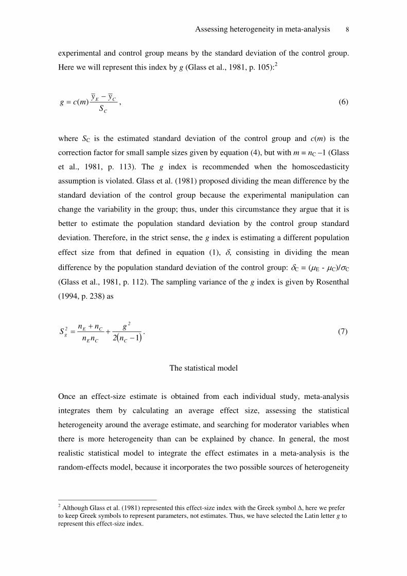
Another effect-size index from the d family is that proposed by Glass et al.

(1981; see also Glass, 1976), consisting of dividing the difference between the


experimental and control group means by the standard deviation of the control group.

Here we will represent this index by g (Glass et al., 1981, p. 105):2

C

CE

S

yymcg

−= )( , (6)

where SC is the estimated standard deviation of the control group and c(m) is the

correction factor for small sample sizes given by equation (4), but with m = nC –1 (Glass

et al., 1981, p. 113). The g index is recommended when the homoscedasticity

assumption is violated. Glass et al. (1981) proposed dividing the mean difference by the

standard deviation of the control group because the experimental manipulation can

change the variability in the group; thus, under this circumstance they argue that it is

better to estimate the population standard deviation by the control group standard

deviation. Therefore, in the strict sense, the g index is estimating a different population

effect size from that defined in equation (1), δ, consisting in dividing the mean

difference by the population standard deviation of the control group: δC = (µE - µC)/σC

(Glass et al., 1981, p. 112). The sampling variance of the g index is given by Rosenthal

(1994, p. 238) as

( )1−+

+=

C

2

CE

CE2g n2

g

nn

nnS . (7)

The statistical model

Once an effect-size estimate is obtained from each individual study, meta-analysis

integrates them by calculating an average effect size, assessing the statistical

heterogeneity around the average estimate, and searching for moderator variables when

there is more heterogeneity than can be explained by chance. In general, the most

realistic statistical model to integrate the effect estimates in a meta-analysis is the

random-effects model, because it incorporates the two possible sources of heterogeneity

2 Although Glass et al. (1981) represented this effect-size index with the Greek symbol ∆, here we preferto keep Greek symbols to represent parameters, not estimates. Thus, we have selected the Latin letter g torepresent this effect-size index.


among the studies in a meta-analysis: first, statistical variability caused by sampling

error and, second, substantive variability.

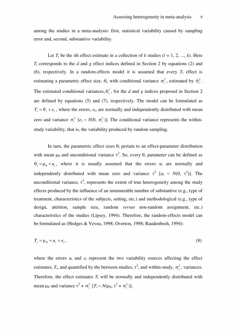
Let Ti be the ith effect estimate in a collection of k studies (i = 1, 2, ..., k). Here

Ti corresponds to the d and g effect indices defined in Section 2 by equations (2) and

(6), respectively. In a random-effects model it is assumed that every Ti effect is

estimating a parametric effect size, θi, with conditional variance 2iσ , estimated by 2

iσ̂ .

The estimated conditional variances, 2iσ̂ , for the d and g indices proposed in Section 2

are defined by equations (5) and (7), respectively. The model can be formulated as

iii eT +θ= , where the errors, ei, are normally and independently distributed with mean

zero and variance 2iσ [ei ∼ N(0, 2

iσ )]. The conditional variance represents the within-

study variability, that is, the variability produced by random sampling.

In turn, the parametric effect sizes θi pertain to an effect-parameter distribution

with mean µθ and unconditional variance τ2. So, every θi parameter can be defined as

i iuθθ = µ + , where it is usually assumed that the errors ui are normally and

independently distributed with mean zero and variance τ2 [ui ∼ N(0, τ2)]. The

unconditional variance, τ2, represents the extent of true heterogeneity among the study

effects produced by the influence of an innumerable number of substantive (e.g., type of

treatment, characteristics of the subjects, setting, etc.) and methodological (e.g., type of

design, attrition, sample size, random versus non-random assignment, etc.)

characteristics of the studies (Lipsey, 1994). Therefore, the random-effects model can

be formulated as (Hedges & Vevea, 1998; Overton, 1998; Raudenbush, 1994):

iii euT ++µ= θ , (8)

where the errors ui and ei represent the two variability sources affecting the effect

estimates, Ti, and quantified by the between-studies, τ2, and within-study, 2iσ , variances.

Therefore, the effect estimates Ti will be normally and independently distributed with

mean µθ and variance τ2 + 2iσ [Ti ∼ N(µθ, τ2 + 2

iσ )].


When there is no true heterogeneity among the effect estimates, then the

between-studies variance is zero (τ2 = 0), and there only will be variability due to

sampling error, which is represented in the model by the conditional within-study

variance, 2iσ . In this case, all the studies estimate one parametric effect size, θi = θ, and

the statistical model simplifies to i iT e= θ+ , thus becoming a fixed-effects model. So,

the fixed-effects model can be considered as a particular case of the random-effects

model when there is no between-studies variability and, as a consequence, the effect

estimates, Ti, are only affected by sampling error, 2iσ , following a normal distribution

with mean θ (being in this case θ = µθ) and variance 2iσ [Ti ∼ N(θ, 2

iσ )] for large

sample sizes.

Assessing the extent of heterogeneity in a meta-analysis helps to decide which of

the two models is the most plausible and this decision affects, at least, the weighting

factor used to obtain an average effect size. The usual estimate of a mean effect size

consists of weighting every effect estimate, Ti, by its inverse variance, wi:

i ii

ii

wTT

w=∑∑

. (9)

In a fixed-effects model, the weighting factor for the ith study is estimated by wi =

1/ 2iσ̂ . In a random-effects model, the weights are estimated by 2 2

i iˆ ˆ1/(τ )w = +σ . For the

d and g indices the estimated within-study variances, 2iσ̂ , are defined in equations (5)

and (7), respectively. A commonly used estimator of the between-studies variance, τ2, is

an estimator based on the method of moments proposed by DerSimonian and Laird

(1986):

≤

>−−

=

1)-(for

1)-(for

0

1)(

τ2

kQ

kQ

c

kQ

ˆ (10)


being c

2i

ii

wc w

w= −∑∑ ∑

(11)

where wi is the weighting factor for the ith study assuming a fixed-effects model (wi =

1/ 2iσ̂ ), k is the number of studies, and Q is the statistical test for heterogeneity proposed

by Cochran (1954) and defined in equation (12). To avoid negative values for 2τ̂ when

Q ≤ (k – 1), 2τ̂ is equated to 0. Note that due to this truncation, 2τ̂ is a biased estimator

for τ 2.

Assessing heterogeneity in meta-analysis

Quantifying the extent of heterogeneity among a collection of studies is one of the most

troublesome aspects of a meta-analysis. It is important because it can affect the decision

about the statistical model to be selected, fixed- or random-effects. On the other hand, if

significant variability is found, potential moderator variables can be sought to explain

this variability.

The between-studies variance, τ2, is the parameter in the statistical model that

mainly represents the true (substantive, clinical) heterogeneity among the true effects of

the studies. Therefore, a good procedure for determining whether there is true

heterogeneity among a collection of studies should be positively correlated with τ2. At

the same time, it should not be affected by the number of studies, and should be scale-

free in order to be comparable among meta-analyses that have applied different effect-

size indices.

The statistical test usually applied in meta-analysis for determining whether

there is true heterogeneity among the studies’ effects is the Q test, proposed by Cochran

(1954) and defined as (Hedges & Olkin, 1985, p. 123, eq. 25):

( )2

i iQ w T T= −∑ , (12)


where wi is the weighting factor for the ith study assuming a fixed-effects model, and T

is defined in equation (9). If we assume that the conditional within-study variances, 2iσ ,

are known3, then under the null hypothesis of homogeneity (Ho: δ1 = δ2 = ... = δk; or

also Ho: τ2 = 0), the Q statistic has a chi-square distribution with k – 1 degrees of

freedom. Thus, Q values higher than the critical point for a given significance level (α)

enable us to reject the null hypothesis and conclude that there is statistically significant

between-study variation.

One problem with the Q statistic is that its statistical power depends on the

number of studies, with power being very low or very high for a small or a large

number of studies, respectively. To solve the problems of the Q statistic and the non

comparability of the between-studies variance, τ2, among meta-analyses with different

effect-size metrics, Higgins and Thompson (2002) have recently proposed the I2 index.

The I2 index quantifies the extent of heterogeneity from a collection of effect sizes by

comparing the Q value to its expected value assuming homogeneity, that is, to its

degrees of freedom (df = k – 1):

≤

>×−−

=1)-(for

1)-(for

0

%1001)(

2

kQ

kQQ

kQ

I (13)

When the Q statistic is smaller than its degrees of freedom, then I2 is truncated to zero.

The I2 index can easily be interpreted as a percentage of heterogeneity, that is, the part

of total variation that is due to between-studies variance, 2τ̂ . Therefore, there is a direct

relationship between 2τ̂ and I2 that can be formalized from the equations (10) and (13)

as,

Q

ˆcI

22 τ= (14)

3 In practice, the population within-study variances never will be known, so they will have to be estimatedfrom the sample data. For example, equations (5) and (7) are used to estimate the within-study variancesfor d and g indices.


To show empirically this relation, Figure 1 presents the results of a simulation,

assuming a random-effects model with δ = 0.5, k = 50, an average sample size N = 50

(nE = nC for every study), and manipulating the parametric between-studies variance, 2τ ,

with values from 0.0 to 0.45, and 5 replications per condition. Figure 1 represents the

obtained values of 2τ̂ and I2 for every replication. So, for the manipulated conditions

2τ̂ values around 0.025, 0.05, and 0.15 correspond to I2 values of 25%, 50%, and 75%,

respectively. Further, note that beyond a certain value of 2τ there is relatively little

increase in I2. In particular, I2 values higher than 85% will subsequently increase only

slightly even if the between-studies variance increases substantially. Therefore, the I2

index seems particularly useful in describing heterogeneity in a meta-analysis with a

medium-to-low between-studies variance, and not so useful for large 2τ values.

Higgins and Thompson (2002) have also developed a confidence interval for I2.

The interval is formulated by calculating another of their proposed measures of

heterogeneity, the H2 index obtained by (Higgins & Thompson, 2002, p. 1545, eq. 6),

QH=

k-2

1, (15)

also known as Birge’s ratio (Birge, 1932). Then they define I2 in terms of H2 by means

of (Higgins & Thompson, 2002, p. 1546, eq. 10),

22

2

1100%

HI

H

−= × . (16)

This allows us to express inferences of H2 in terms of I2. For practical

application, Higgins and Thompson (2002, p. 1549) recommend a confidence interval

for the natural logarithm of H, ln(H), assuming a standard normal distribution, that

implies the Q statistic and k, given by,

[ ]{ }/ 2exp ln( ) SE ln( )H z Hα± , (17)

where |zα/2| is the (α/2) quantile of the standard normal distribution, and SE[ln(H)] is the

standard error of ln(H) and is estimated by


[ ]2

1 ln( ) ln( 1)if

2 (2 ) (2 3)SE ln( )

1 11 if

2( 2) 3( 2)

Q kQ k

Q kH

Q kk k

− − > − −= − ≤ − −

(18)

The confidence limits obtained by equation (15) are in terms of the H index.

Consequently, they can be easily translated into the I2 metric by applying equation (16)

to both confidence limits.

An example will help to illustrate the calculations for the Q statistic and the I2

index. Figure 2 presents some of the results of a meta-analysis about the effectiveness of

delinquent rehabilitation programs (Redondo, Sánchez-Meca, & Garrido, 1999). In

particular, Figure 2 presents the results of eight studies that compared a control group

with one of two different correctional programs: three studies that compared a control

group with a cognitive-behavioral treatment (CBT) and five studies that compared a

control group with a therapeutic community program (TC). The comparisons were

measured by the d index such as it is defined by equation (2). The purpose of the

example is to illustrate the problems of the Q statistic and how the I2 index is able to

solve them.

As Figure 2 shows, the forest plot for the two groups of studies (the three studies

for CBT and those for TC) reflect high heterogeneity in both cases, but heterogeneity is

more pronounced for CBT studies than for TC studies. In fact, the estimated between-

studies variance, 2τ̂ , for CBT is clearly higher than for TC (0.24 and 0.06, respectively).

However, the Q statistic is very similar and statistically significant in both cases [CBT:

Q(2) = 11.647, p = .003; TC: Q(4) = 11.931, p = .018]. Thus, a direct comparison of the

two Q values is not justified because their degrees of freedom differ, and can

erroneously lead to the conclusion that the two groups of studies are similarly

heterogeneous. But if we calculate the I2 index for both groups, then differences in the

extent of heterogeneity are clearly apparent: whereas CBT studies present an I2 value of

82.8%, implying high heterogeneity, the TC studies present an I2 value of medium size

(66.5%). Thus, the I2 index has been able to reflect differences in the degree of


heterogeneity between two groups of studies when the Q statistic offers very similar

results for them.

The Q statistic is only useful for testing the existence of heterogeneity, but not

the extent of heterogeneity. The I2 index quantifies the magnitude of such heterogeneity

and, if a confidence interval is calculated for it, then it can also be used for testing the

heterogeneity hypothesis. In the example, the confidence limits obtained for the I2 index

applying equation (15) were for CBT studies from 47.6% to 94.4%, and for TC studies

from 12.7% to 87.1%. In both cases, the 0% value is not contained by the confidence

interval, showing the existence of heterogeneity and coinciding with the results obtained

with the Q statistic. On the other hand, the width of the I2 CI informs about the accuracy

of the true heterogeneity estimation. Thus, as the number of CBT studies is higher than

that of TC studies its true heterogeneity estimation is more accurate (confidence width =

46.8% and 74.4%, respectively). Therefore, the I2 index with its confidence interval can

substitute for the Q statistic, because it offers more information.

To further show the usefulness of the I2 index to compare the extent of

heterogeneity among different meta-analyses, Table 1 presents the results of four meta-

analyses about treatment outcome in the social and behavioral sciences, in terms of their

Q tests and I2 indices. As every meta-analysis has a different number of studies (k), the

Q values are not comparable. However, the I2 indices enable to assess the extent of true

heterogeneity as a percentage of total variation. So, for the three first meta-analyses

their respective Q values only inform about the existence of heterogeneity, while the I2

values allow us to identify the Sánchez-Meca et al. (1999) meta-analysis as showing the

largest heterogeneity (I2 = 90.8%; 95% CI: 88.6% and 92.9%), in comparison to the

other two (I2 = 67.3%, 95% CI: 57% and 75.2%; and I2 = 74.2%; 95% CI: 64.8% and

82.3%). On the other hand, the only meta-analysis with a nonsignificant Q test

coincides with a I2 = 0%.

Method

The simulation study was programmed in GAUSS (Aptech Systems, 1992). For

simulating each individual study, we have assumed a two-groups design (experimental

versus control) and a continuous outcome. Two different effect-size indices, both


pertaining to the d metric, were defined: the standardized mean difference d index

defined by Hedges and Olkin (1985) and the g index proposed by Glass et al. (1981).

The main difference between them is the standard deviation used, as noted above.

To simulate a collection of k single studies we assumed a random-effects model.

Thus, from a normal distribution of parametric effect sizes, θi, with mean µθ = 0.5 and

between-studies variance τ2 [θi ∼ N(0.5, τ2)], collections of k studies were randomly

generated. The mean effect-size parameter was fixed at µθ = 0.5, as it can be considered

an effect of medium magnitude (Cohen, 1988).4 Once a θi value was randomly selected,

two distributions (for the experimental and control groups) were generated, with means

µE = θi and µC = 0, variance for the control group equal to 1 (σC2 = 1) and variance for

the experimental group equal 1, 2, or 4 (σE2 = 1, 2, or 4), depending on the ratio

between σE2 and σC

2. The distributions for scores in experimental and control groups

might be normal or non-normal, with different values of skewness and kurtosis in the

non-normal cases. Then, two random samples (experimental and control) were selected

from the two distributions with sizes nE = nC, and the means ( Ey and Cy ) and standard

deviations (SE and SC) were obtained. Thus, the standardized mean differences, d (eq. 2)

and g (eq. 6), and their sampling variances, Sd2 (eq. 5) and Sg

2 (eq. 7), were calculated.

The calculations for the d and g indices, and their sampling variances, were repeated for

each one of the k studies of each simulated meta-analysis. Then, for every set of effect

estimates (d and g indices), the calculations to obtain the Q statistic with its statistical

significance and the I2 index with its confidence interval were carried out, applying

equations (11), (12), and (15), respectively. Thus, the following factors were

manipulated in the simulations:

(a) The between-studies variance, τ2, with values 0, 0.04, 0.08, and 0.16. When τ2 =

0, the statistical model becomes a fixed-effects model, because there is no

between-studies variance. The selected values of τ2 were similar to those used

in other simulation studies (Biggerstaff & Tweedie, 1997; Brockwell & Gordon,

2001; Erez et al., 1996; Field, 2001; Hedges & Vevea, 1998; Overton, 1998).

4 Additional simulations varying the value of µθ showed similar results to that of µθ = 0.5 for the Qstatistic and the I2 index. Thus, we maintained fixed µθ to simplify the simulation design.


(b) The number of studies for each meta-analysis, k, with values 5, 10, and 20.

These values for k are common in real meta-analyses and they were selected to

study the performance of Q and I2 when the number of studies is small, because

the literature suggests poor performance under these conditions (Hardy &

Thompson, 1998; Harwell, 1997; Sánchez-Meca & Marín-Martínez, 1997).

(c) The within-study variances for experimental and control groups were varied

using ratios for experimental and control groups, respectively, of 1:1, 2:1, and

4:1 as suggested in the literature (e.g., McWilliams, 1991; Wilcox, 1987). The

variance of the experimental group was increased in comparison to that of the

control group because increases in variability are more plausible when there is

experimental manipulation (e.g., a psychological treatment) (Glass et al., 1981).

(d) Usually, the studies integrated in a meta-analysis have different sample sizes.

Thus, the mean sample size for each generated meta-analysis was varied with

values N = 30, 50, and 80. The sample-size distribution used in the simulations

was obtained by a review of the meta-analyses published in 18 international

psychological journals. This review enabled us to obtain a real sample-size

distribution characterized by a Pearson skewness index of +1.464 (more

detailed information is given in Sánchez-Meca & Marín-Martínez, 1998). In

accord with this value, three vectors of five Ns each were selected averaging 30,

50, or 80, with the skewness index given above to approximate real data: [12,

16, 18, 20, 84], [32, 36, 38, 40, 104], and [62, 66, 68, 70, 134]. Each vector of

Ns was then replicated either 2 or 4 times for meta-analyses of k = 10 and 20

studies, respectively. The within-study sample sizes for the experimental and

control groups were equal (nE = nC , being N = nE + nC, for each single study).

For example, the sample sizes vector [12, 16, 18, 20, 84] means that the

experimental and control group sample sizes were, respectively, [nE = nC = 6, 8,

9, 10, 42].

(e) Scores for the experimental and control participants in each pseudo-study were

generated assuming a variety of different distributions: both normal

distributions and non-normal distributions. To generate non-normal

distributions, the normality pattern was manipulated to obtain skewed

distributions by means of the Fleishman (1978) algorithm, with the following

values of skewness/kurtosis: 0.5/0, 0.75/0, and 1.75/3.75. These values of


skewness and kurtosis can be considered of a moderate magnitude (DeCarlo,

1997; Hess, Olejnik, & Huberty, 2001).

To simplify the design of the simulation study we did not cross all of the

manipulated factors. In the condition of normal distributions for the experimental and

control groups in the single studies, we crossed all the factors mentioned above,

obtaining a total of 4 (τ2 values) x 3 (k values) x 3 (variance ratios) x 3 ( N values) =

108 conditions. For the three conditions in which the score distributions of the single

studies were non-normal, the design of the simulation was simplified by reducing the

number of studies in each meta-analysis to only two conditions: k = 5 and 20. Thus, the

number of conditions was 3 (τ2 values) x 2 (k values) x 3 (variance ratios) x 3 ( N

values) x 3 (non-normal distributions) = 162. Therefore, the total number of

manipulated conditions was 108 (normal distributions) + 162 (non-normal distributions)

= 270 conditions. For each of the 270 conditions, 10,000 replications were generated.

To obtain estimates of the Type I error rate and statistical power for the Q statistic and

the confidence interval for the I2 index, assuming a significance level of α = .05, the

following computations over the 10,000 replications in each condition were carried out,

(a) In conditions where the between-studies variance was zero (τ2 = 0), the

proportion of false rejections of the null hypothesis of homogeneity in the

10,000 replications was the empirical Type I error rate for the Q statistic.

Similarly, the proportion of replications in which the confidence interval for

I2 did not contain the value τ2 = 0 represented its empirical Type I error rate.

Following Cochran (1952) we assumed that good control of the Type I error

rate for α = 0.05 implies empirical rates in the range 0.04-0.06.

(b) In conditions with non zero between-studies variance (τ2 > 0), the proportion

of rejections of the homogeneity hypothesis was the empirical power for the

Q statistic, and the proportion of replications in which the confidence interval

for I2 did not contain the value τ2 = 0, was an estimate of the power of this

procedure. Following Cohen (1988), we adopted 0.80 as the minimum

advisable power.


Results

First, we will present the results obtained through the manipulated conditions in respect

to the control of Type I error rates achieved by the Q test and the confidence interval of

I2 (I2 CI) both for the d and g indices. Then, the results in terms of statistical power will

be shown.5

Type I error rate.

Estimated Type I error rates were obtained when the between-studies variance was zero

(τ2 = 0). For each condition, the Type I error rate was calculated dividing by 10,000 the

number of replications in which the null hypothesis was incorrectly rejected using the Q

test, or the number of replications in which the value zero was not in the I2 CI. Figure 3

presents results for Type I error rates as a function of the number of studies and the

average sample size under the conditions assuming normality and homoscedasticity in

the experimental and control groups’ distributions. As Figure 3 shows, good control of

the Type I error rate is achieved with both the Q test and the I2 CI when the d index is

used, but not with the g index. The good control of the Type I error for Q and I2 CI with

the d index is neither affected by the number of studies nor by the average sample size

in the meta-analysis. However, note that the Type I error rate for I2 CI with the d index

is slightly lower than the .04 limit that we have assumed as representing a good

adjustment to the .05 nominal significance level. On the other hand, with the g index, Q

and I2 CI present Type I error rates clearly higher than the nominal α = .05, and

importantly above the .06 limit. This poor performance slightly increases with the

number of studies, but diminishes with the average sample size.

When the experimental- and control-group distributions were normal but the

homoscedasticity assumption was not met, both Q and I2 CI maintained good control of

the Type I error rate with the d index (although the Type I error rate for I2 CI being

slightly under the .04 limit). This result was not affected by the number of studies and

the average sample size, as Figure 4 shows. However, with the g index, a dramatic

increase of the Type I error rate for Q and I2 CI was found as the ratio between


experimental and control groups’ variances was increased. As Figure 4 shows, the poor

performance of Q and I2 CI for the g index is affected by the number of studies and the

average sample size, with trends similar to those obtained assuming normality and

homoscedasticity.

When the experimental- and control-group distributions were non-normal and

the homoscedasticity assumption was met, the control of the Type I error rate was good

for both the Q test and I2 CI computed for the d index. However, as the distributions

deviated from normality, the Type I error rates of Q and the I2 CI for the g index

suffered a drastic increase. Finally, when the normality and homoscedasticity

assumptions were not met, the Type I error rates of Q and I2 CI for the d index

maintained their proximity to the nominal α = .05, whereas the performance of Q and I2

CI for the g index remained very poor (see Figure 5).

Statistical power.

The estimated power values were obtained when between-studies variance was higher

than zero (τ2 > 0). For each condition, the power value was calculated by dividing by

10,000 the number of replications in which the null hypothesis is correctly rejected

using the Q test, or the number of replications in which the zero value was not in the

confidence interval of I2.

Figure 6 shows the estimated power values when the normality and

homoscedasticity assumptions were met, as a function of the number of studies and the

between-studies variance. As expected, the estimated power for all of the procedures

increased as the number of studies and the between-studies variance increased. The

results also showed that the recommended 0.8 power value (Cohen, 1988) was reached

only when there were 20 or more studies and a large between-studies variance (τ2 ≥

0.16). Similar power results were obtained as a function of the average sample size.

With normal distributions and heteroscedastic variances the power values for Q

and I2 CI showed similar trends as a function of the number of studies: the higher the

number of studies the higher the power (see Figure 7). Although the trend was similar

5 Because of space limitations, not all of the tables and figures for all of the manipulated conditions are


for all of the procedures, Q and I2 CI achieved a higher power when the g index was

used in comparison with the d index. The better power obtained with the g index under

heterogeneous variances occurred because g uses the control group standard deviation,

whereas the d index uses a pooled standard deviation obtained from the experimental

and control groups. In our simulations we assumed, as Glass suggested (Glass et al.,

1981), control-group standard deviations smaller than those of the experimental groups.

This circumstance leads to higher heterogeneity among g indices than among d indices.

As a consequence, it is easier for Q and I2 CI to detect heterogeneity among g indices.

Finally, similar power results were obtained when the normality and homoscedasticity

assumptions were not met. As Figure 8 shows, Q and I2 CI achieved higher power

values with the g index than with the d index. However, the inflated Type I error rates

obtained with the g index implies an inappropriate performance of Q and I2 CI with this

index.

Discussion

Traditionally, the Q test has been the normal procedure in assessing the heterogeneity

hypothesis in meta-analysis (Cooper & Hedges, 1994). Recently, a new statistic named

I2, and a confidence interval around it, has been proposed to estimate the extent of

heterogeneity, as well as its statistical significance (Higgins & Thompson, 2002;

Higgins et al., 2003). Assessing heterogeneity in meta-analysis is a crucial issue because

the meta-analyst’s decision to select the statistical model to be applied in a meta-

analysis (fixed- versus random-effects model) can be affected by the result of a

homogeneity test. Due to the importance of this issue, the purpose of this paper was to

compare the performance of two procedures, the Q test and I2 CI, to assess the

heterogeneity among a set of single studies in a meta-analysis. In particular, Type I error

rates and statistical power of the two procedures were examined by means of Monte

Carlo simulation as a function of the number of studies, the average sample size, the

between-studies variance, and the normality and homoscedasticity of the experimental-

and control-group distributions. On the other hand, two different effect-size indices

pertaining to the d family were used to calculate the Q test and the I2 CI: d and g

indices. A comparison between the Q test and the I2 CI has not yet been carried out.

presented. Interested readers can request the complete set of tables and figures from the authors.


Therefore, the results of our study cast some light on the performance of both

procedures in assessing heterogeneity in a meta-analysis.

The results of the simulation study helped us reach several conclusions related to

our goals. In respect to the control of Type I error rate, the performance of the Q test

and the I2 CI was very similar. In fact, there were more differences between the

procedures based on d and g indices than between the Q test and the I2 CI. In particular,

with the d index both procedures achieved good control of the Type I error rate, whereas

the performance of the Q test and the I2 CI calculated with the g index was very poor.

On the other hand, Type I error rates for both procedures with the d index were not

affected by the number of studies and the average sample size. However, the

performance of the Q test and the I2 CI depend on the effect-size metric. Therefore,

confidence intervals around I2 obtained from meta-analyses with different effect-size

metrics should be interpreted cautiously, because they may not be comparable.

In respect to statistical power, there were no notable differences between the Q

test and the I2 CI. As expected, both procedures exhibited higher power as the number

of studies, the average sample size, and the between-studies variance increased.

However, with a small number of studies (k < 20) and/or average of sample size ( N <

80), the power is under the minimum advisable value 0.8. In fact, both procedures

calculated with the d index reached power values as small as 0.3 in some conditions.

Therefore, the I2 CI suffers the same problem as the Q test in terms of statistical power.

On the other hand, the power of these procedures calculated with the g index

was higher than that obtained with the d index. However, the highest power for

summaries of the g index was achieved at the expense of an inadmissibly large Type I

error rate. Therefore, the performance of the Q test and I2 CI with the g index is poor. In

any case, the usefulness of our results for the g index should be limited to real meta-

analyses where systematically the variability in the experimental groups is higher than

that of the control groups; this only will happen when the implementation of a treatment

produces an overdispersion of the subject scores in comparison to the control group

scores. The poor Type I error performance of the Q test and the I2 index with g index

under normality and homoscedasticity raises various concerns, including the accuracy

of the sampling variance of this index. Our results also show a negligible effect on the


Type I error rates and statistical power of the Q test and the I2 CI with the d index when

the usual assumptions about the experimental- and control-group distributions

(normality and homoscedasticity) are not met.

In summary, our findings show that the I2 CI performs in a similar way to the Q

test from an inferential point of view. But the I2 index has important advantages in

respect to the classical Q test. First, it is easily interpretable because it is a percentage

and does not depend on the degrees of freedom. Another advantage is that it provides a

way of assessing the magnitude of the heterogeneity in a meta-analysis, whereas the Q

test reports about the statistical significance of the homogeneity hypothesis. On the

other hand, the I2 CI informs about the accuracy of the true heterogeneity estimation.

In addition, the I2 index can be used to assess the degree of misspecification

error when a qualitative moderator variable is tested. In particular, for every category of

the moderator variable, an I2 index can be calculated and their values are directly

compared in order to determine which categories show a good fit to the statistical model

and which ones do not. On the other hand, the I2 index can be useful to compare the

fitting of alternative models with different moderator variables regardless of their

degrees of freedom. Future research in this area can help to ascertain the usefulness of

the I2 index when the statistical model in a meta-analysis includes moderator variables.

Some warnings for the use of the I2 index have to be taken into account. The

confidence interval around I2 used to assess the homogeneity hypothesis in meta-

analysis suffers the same problems of low power that the Q test does when the number

of studies is small. The I2 CI does not solve the shortcomings of the Q test. Therefore,

using either the I2 CI or the Q test to decide upon the statistical model (fixed- versus

random-effects model) in a meta-analysis can be misleading. With a small number of

studies (k < 20) both the I2 CI and the Q test should be interpreted very cautiously.

As the I2 index and its confidence interval allow us to assess simultaneously both

the statistical significance and the extent of heterogeneity, the meta-analyst can obtain a

more complete picture of heterogeneity than that offered by the Q test. Therefore, we

propose using I2 and its confidence interval to assess heterogeneity in meta-analysis,


although taking into account its low statistical power when the number of studies is

small.

On the other hand, our results comparing the d and g indices have shown very

different performances for the I2 CI depending on the effect-size metric. Under our

manipulated conditions, the g index systematically showed an inappropriate control of

the Type I error rate and, therefore, using the Q test or the I2 CI with this index is

unadvisable. However, the poor performance that we have found for the Q test and the

I2 CI with the g index is only applicable when the studies systematically present a

higher variability in the experimental group than in the control group. More research

should be carried out to study the comparability of the I2 index with other effect-size

metrics, such as correlation coefficients, odds ratios, and so on. Finally, it should be

noted that the results of our study are limited to the simulated conditions. Consequently,

additional research efforts manipulating other factors, or examining different levels of

these factors, can help to assess the generalizability of our findings.

References

Alexander, R. A., Scozzaro, M. J., & Borodkin, L. J. (1989). Statistical and empirical

examination of the chi-square test for homogeneity of correlations in meta-

analysis. Psychological Bulletin, 106, 329-331.

Aptech Systems, Inc. (1992). The GAUSS system (Vers. 3.0). Kent, WA: Author.

Biggerstaff, B. J., & Tweedie, R. L. (1997). Incorporating variability estimates of

heterogeneity in the random effects model in meta-analysis. Statistics in

Medicine, 16, 753- 768.

Birge, R. T. (1932). The calculation of errors by the method of least squares. Physical

Review, 40, 207-227.

Brockwell, S. E., & Gordon, R. I.(2001) A comparison of statistical methods for meta-

analysis. Statistics in Medicine, 20, 825- 840.

Cochran, W. G. (1952). The χ2 test of goodness of fit. Annals of Mathematical

Statistics, 23, 315-345.

Cochran, W. G. (1954). The combination of estimates from different experiments.

Biometrics, 10, 101-129.


Cohen, J. ( 1988). Statistical power analysis for the behavioral sciences (2nd ed.). New

York: Academic Press.

Cooper, H. (1998). Integrating research: A guide for literature reviews (3rd ed.).

Newbury Park, CA: Sage.

Cooper, H., & Hedges, L. V. (Eds.). (1994). The handbook of research synthesis. New

York: Russell Sage Foundation.

Cornwell, J. M. (1993). Monte Carlo comparison of three tests for homogeneity of

independent correlations. Educational & Psychological Measurement, 53, 605-

618.

Cornwell, J. M., & Ladd, R. T. (1993). Power and accuracy of the Schmidt and Hunter

meta-analytic procedures. Educational & Psychological Measurement, 53, 877-

895.

DeCarlo, L. T. (1997). On the meaning and use of kurtosis. Psychological Methods, 2,

292-306.

DerSimonian, R., & Laird, N. (1986) Meta-analysis in clinical trials. Controlled

Clinical Trials, 7, 177-188.

Egger, M., Smith, G. D., & Altman, D. G. (Eds.). (2001). Systematic reviews in health

care: Meta-analysis in context (2nd ed.). London: BMJ Publishing Group.

Erez. A., Bloom, M. C., & Wells, M. T. (1996). Using random rather than fixed effects

models in meta-analysis: Implications for situational specificity and validity

generalization. Personnel Psychology, 49, 275-306.

Field, A. P. (2001). Meta-analysis of correlation coefficients: A Monte Carlo

comparison of fixed- and random-effects methods. Psychological Methods, 6,

161-180.

Field, A. P. (2003). The problems in using fixed-effects models of meta-analysis on

real-world data. Understanding Statistics, 2, 77-96.

Fleishman, A. I. (1978). A method for simulating nonnormal distributions.

Psychometrika, 43, 521-531.

Glass, G. V. (1976). Primary, secondary, and meta-analysis of research. Educational

Research, 5, 3-8.

Glass, G. V., McGaw, B., & Smith, M. L. (1981). Meta-analysis in social research.

Newbury Park, CA: Sage.

Hardy, R. J., & Thompson, S. G. (1996). A likelihood approach to meta-analysis with

random effects. Statistics in Medicine, 15, 619-629.


Hardy, R. J., & Thompson, S. G. (1998). Detecting and describing heterogeneity in

meta-analysis. Statistics in Medicine, 17, 841-856.

Harwell, M. (1997). An empirical Study of Hedge’s homogeneity test. Psychological

Methods, 2, 219-231.

Hedges, L. V. (1994). Fixed effects models. In H. Cooper & L. V. Hedges (Eds.), The

handbook of research synthesis (pp. 285-299). New York: Russell Sage

Foundation.

Hedges, L. V., & Olkin, I. (1985). Statistical methods for meta-analysis. Orlando, FL:

Academic Press.

Hedges, L. V., & Vevea, J. L. (1998). Fixed- and random-effects models in meta-

analysis. Psychological Methods, 3, 486-504.

Hess, B., Olejnik, S., & Huberty, C. J. (2001). The efficacy of two improvement-over-

chance effect sizes for two-group univariate comparisons under variance

heterogeneity and nonnormality. Educational & Psychological Measurement,

61, 909-936.

Higgins, J. P. T., & Thompson, S. G. (2002). Quantifying heterogeneity in a meta-

analysis. Statistics in Medicine, 21, 1539-1558.

Higgins, J. P. T., Thompson, S. G., Deeks, J. J., & Altman, D. G. (2003). Measuring

inconsistency in meta-analyses. British Medical Journal, 327, 557-560.

Hunter, J. E., & Schmidt, F. L. (2000). Fixed effects vs random effects meta-analysis

models: Implications for cumulative research knowledge. International Journal

of Selection & Assessment, 8, 275-292.

Hunter, J. E., & Schmidt, F. L. (2004). Methods of meta-analysis: Correcting error and

bias in research findings (2nd ed.). Newbury Park, CA: Sage.

Lipsey, M. W. (1994). Identifying potentially interesting variables and analysis

opportunities. In H. Cooper & L. V. Hedges (Eds.), The handbook of research

synthesis (pp. 111-123). New York: Russell Sage Foundation.

McWilliams, L. (1991, April). Variance heterogeneity in empirical studies in education

and psychology. Paper presented at the annual colloquium of the American

Educational Research Association, San Francisco.

Moreno, P. J., Méndez, F. X., & Sánchez-Meca, J. (2001). Effectiveness of cognitive-

behavioural treatment in social phobia: A meta-analytic review. Psychology in

Spain, 5, 17-25.


National Research Council. (1992). Combining information: Statistical issues and

opportunities for research. Washington, DC: National Academy Press.

Osburn, H. G., Callender, J. C., Greener, J. M., & Ashworth, S. (1983). Statistical

power of tests of the situational specificity hypothesis in validity generalization

studies: A cautionary note. Journal of Applied Psychology, 68, 115-122.

Overton, R. C. (1998). A comparison of fixed-effects and mixed (random-effects)

models for meta-analysis tests of moderator variable effects. Psychological

Methods, 3, 354-379.

Paul, S. R., & Donner, A. (1992). Small sample performance of tests of homogeneity of

odds ratios in K 2x2 tables. Statistics in Medicine, 11, 159-165.

Raudenbush, S. W. (1994). Random effects models. In H. Cooper and L. V. Hedges

(Eds.), The handbook of research synthesis (pp. 301-321). New York: Russell

Sage Foundation.

Redondo, S., Garrido, V., & Sánchez-Meca, J. (1997). What works in correctional

rehabilitation in Europe: A meta-analytic review. In S. Redondo, V. Garrido, J.

Pérez, & R. Barberet (Eds.), Advances in psychology and law: International

contributions (pp. 499-523). Berlin: De Gruyter.

Redondo, S., Sánchez-Meca, J., & Garrido, V. (1999). The influence of treatment

programs on the recidivism of juvenile and adult offenders: An European meta-

analytic review. Psychology, Crime & Law, 5, 251-278.

Rosenthal, R. (1991). Meta-analytic procedures for social research (rev. ed.). Newbury

Park, CA: Sage.

Rosenthal, R. (1994). Parametric measures of effect size. In H. Cooper and L. V.

Hedges (Eds.), The handbook of research synthesis (pp. 231-244). New York:

Russell Sage Foundation.

Sackett, P. R., Harris, M. M., & Orr, J. M. (1986). On seeking moderator variables in

the meta-analysis of correlational data: A Monte Carlo investigation of statistical

power and resistance to Type I error. Journal of Applied Psychology, 71, 302-

310.

Sagie, A., & Koslowsky, M. (1993). Detecting moderators with meta-analysis: An

evaluation and comparison of techniques. Personnel Psychology, 46, 629-640.

Sánchez-Meca, J., & Marín-Martínez, F. (1997). Homogeneity tests in meta-analysis: A

Monte Carlo comparison of statistical power and Type I error. Quality &

Quantity, 31, 385-399.


Sánchez-Meca, J., & Marín-Martínez, F. (1998). Weighting by inverse variance or by

sample size in meta-analysis: A simulation study. Educational & Psychological

Measurement, 58, 211-220.

Sánchez-Meca, J., Olivares, J., & Rosa, A.I. (1999). The problem of tobacco addiction:

Meta-analysis of behavioural treatments in Spain. Psychology in Spain, 3, 36-45.

Shadish, W. R., & Haddock, C. K. (1994). Combining estimates of effect size. In H.

Cooper & L. V. Hedges (Eds.), The handbook of research synthesis (pp. 261-

281). New York: Russell Sage Foundation.

Spector, P. E., & Levine, E. L. (1987). Meta-analysis for integrating study outcomes: A

Monte Carlo study of its susceptibility to Type I and Type II errors. Journal of

Applied Psychology, 72, 3-9.

Sutton, A. J., Abrams, K. R., Jones, D. R., Sheldon, T. A., & Song, F. (2000). Methods

for meta-analysis in medical research. Chichester, UK: Wiley.

Whitehead, A. (2002). Meta-analysis of controlled clinical trials. Chichester, UK:

Wiley.

Wilcox, R. R. (1987). New designs in analysis of variance. Annual Review of

Psychology, 38, 29-60.


Table 1. Q tests and I2 indices for several meta-analyses.

Source Issue k Q p I295% C I

Ll – Lu

Redondo, Garrido, &Sánchez-Meca(1997)

Correctional treatmentoutcome

57 171.27 <.0001 67.3% 56.96% - 75.16%

Redondo, Sánchez-Meca, & Garrido(1999)

Correctional treatmentoutcome

32 124.07 <.0001 74.2% 64.82% - 82.26%

Sánchez-Meca,Olivares, & Rosa(1999)

Tobacco addictiontreatment outcome

36 389.07 <.0001 90.8% 88.55% - 92.93%

Moreno, Méndez, &Sánchez-Meca(2000)

Social phobia treatmentoutcome

39 19.163 >.05 0% -

k: number of studies. Q: homogeneity test. p: probability level associated to the Q test. I2: I2 index. 95%CI: 95% confidence interval around I2. Ll and Lu: lower and upper confidence limits for I2.


Figure 1. Results of the simulation relating I2 values to estimated between-studies variance.

0,00 0,05 0,10 0,15 0,20 0,25 0,30 0,35 0,40 0,45 0,50

0

25

50

75

100I2

Ind

ex

Between-studies variance τ2


Figure 2. Forest plot of three studies for cognitive-behavioral treatment (CBT) and five studies for

therapeutic community (TC). N1 and N2: sample sizes for treatment and control groups, respectively.

Effect: standardized mean difference following equation (2) (d index). StdErr: standard error of the d

index, obtained by calculating the square root of the equation (5). Filled circles represent the individual

effect size for every study; the boxes refer to the average effect sizes for CBT studies, TC studies, and all

of the studies; the horizontal lines around the circles and boxes indicate the width of confidence intervals;

and the central vertical line represents the null effect size.

Type Citation N1 N2 Effect StdErr

CBT Study 1 64 106 ,14 ,16CBT Study 2 29 29 1,22 ,29CBT Study 3 38 38 ,64 ,24

CBT (3) 131 173 ,46 ,12

TC Study 4 280 834 ,26 ,07TC Study 5 42 38 ,10 ,22TC Study 6 12 12 ,69 ,42TC Study 7 70 61 ,65 ,18TC Study 8 61 61 -,17 ,18

TC (5) 465 1006 ,25 ,06

Combined (8) 596 1179 ,29 ,05

-2,00 -1,00 0,00 1,00 2,00

Favors Control Favors Treatment


(a) (b)

Figure 3. Type I error rates when normality and homogenous variances for experimental and control

groups are assumed as a function of: (a) the number of studies, and (b) the sample size, for the Q statistic

using d index by Hedges (QH), and g index by Glass (QG), and for the confidence interval of I2 with d by

Hedges (I2H), and g by Glass (I2G) indexes.

0 5 10 15 20 25Number of Studies

0.0

0.05

0.10

0.15

0.20

0.25

0.30

Typ

eIE

rror

Ra

tes

I2H

QHI2G

QG

20 30 40 50 60 70 80 90 100Sample Size

0.0

0.05

0.10

0.15

0.20

0.25

0.30

Typ

eIE

rror

Ra

tes

I2H

QHI2G

QG


(a) (b)

Figure 4. Type I error rates when normality and heterogeneous variances for experimental and control

groups (ratio EG:CG = 2:1) are assumed as a function of: (a) the number of studies and (b) the sample

size, for the Q statistic using d index by Hedges (QH), and g index by Glass (QG), and for the confidence

interval of I2 using d index by Hedges (I2H), and g index by Glass (I2G).


0.0

0.15

0.30

0.45

0.60

Typ

eIE

rro

rR

ate

s

I2HQHI2G

QG

20 30 40 50 60 70 80 90 100Sample Size

0.0

0.15

0.30

0.45

0.60

Typ

eIE

rror

Rat

es

I2HQHI2GQG


0.5;0 0.75;0 1.75;3.75Skewness; Kurtosis

0.0

0.2

0.4

0.6

0.8

1.0

Typ

eIE

rror

Rat

es

I2H

QHI2G

QG

0.5;0 0.75;0 1.75;3.75Skewness; Kurtosis

0.0

0.2

0.4

0.6

0.8

1.0

Typ

eIE

rror

Rat

es

I2HQHI2GQG

(a) Variance ratio EG:CG = 2:1 (b) Variance ratio EG:CG = 4:1

Figure 5. Type I error rates when non-normality and heterogeneous variances for experimental and

control groups are assumed as a function of the levels of skewness and kurtosis, using a variance ratio of:

(a) EG:CG= 2:1 and (b) EG:CG= 4:1, for the Q statistic using d index by Hedges (QH), and g index by

Glass (QG), and for the confidence interval of I2 using d index by Hedges (I2H), and g index by Glass

(I2G).


(a) τ2 = 0.04 (b) τ2 = 0.16

Figure 6. Power values rates when normality and homogenous variances for experimental and control

groups are assumed as a function of the number of studies when: (a) τ2 = 0.04, and (b) τ2 = 0.16, for the Q

statistic using d index by Hedges (QH), and g index by Glass (QG), and for the confidence interval of I2

using d index by Hedges (I2H), and g index by Glass (I2G).


0.0

0.2

0.4

0.6

0.8

1.0

Pow

er

Va

lues

Ra

tes

I2H

QHI2G

QG


0.0

0.2

0.4

0.6

0.8

1.0

Pow

er

Va

lues

Ra

tes

I2H

QHI2G

QG


(a) Variance ratio EG:CG = 2:1 (b) Variance ratio EG:CG = 4:1

Figure 7. Power values rates (τ2 = 0.08) when normality and heterogeneous variances for experimental

and control groups are assumed as a function of the number of studies when: (a) ratio EG:CG = 2:1 (b)

ratio EG:CG = 4:1, for the Q statistic using d index by Hedges (QH), and g index by Glass (QG), and for

the confidence interval of I2 using d index by Hedges (I2H), and g index by Glass (I2G).


0.0

0.2

0.4

0.6

0.8

1.0

Pow

erV

alu

esR

ate

s

I2H

QHI2G

QG


0.0

0.2

0.4

0.6

0.8

1.0

Pow

er

Val

ues

Ra

tes

I2H

QHI2G

QG


(a) τ2 = 0.04 (b) τ2 = 0.16

Figure 8. Power values rates when no normality and heterogeneous variances for experimental and

control groups (ratio EG:CG = 2:1) are assumed as a function of levels of skewness and kurtosis when:

(a) τ2 = 0.04 y (b) τ2 = 0.16, for the Q statistic using d index by Hedges (QH), and g index by Glass (QG),

and for the confidence interval of I2 using d index by Hedges (I2H), and g index by Glass (I2G).

0.5;0 0.75;0 1.75;3.75Skewness ; Kurtosis

0.0

0.2

0.4

0.6

0.8

1.0

Pow

er

Val

ues

Rat

es

I2H

QHI2G

QG

0.5;0 0.75;0 1.75;3.75Skewness ; Kurtosis

0.0

0.2

0.4

0.6

0.8

1.0

Pow

er

Val

ues

Rat

es

I2H

QHI2G

QG

Assessing heterogeneity in meta-analysis: Q statistic or I2 index?

Documents

Transcript of Assessing heterogeneity in meta-analysis: Q statistic or I2 index?