CIP – Climate Impacts and Policy Division

WORKING PAPER N. 02.2007

Assessing Climate Change Impacts: Agriculture

Francesco Bosello Dip. di Scienze Economiche Aziendali e Statistiche Università Statale di

Milano, Fondazione Eni Enrico Mattei and Climate Impacts and Policy Division, CMCC

Jian Zhang EEE Program, Abdus Salam International Center of Theoretical Physics

July 2005

Assessing Climate Change Impacts: Agriculture Summary The economy-wide implications of climate change on agricultural sectors in 2050 are estimated using a static computable general equilibrium model. Peculiar to this exercise is the coupling of the economic model with a climatic model forecasting temperature increase in the relevant year and with a crop-growth model estimating climate change impact on cereal productivity. The main results of the study point out on the one hand the limited influence of climate change on world food supply and welfare; on the other hand its important distributional consequences as the stronger negative effects are concentrated on developing countries. The simulation exercise is introduced by a survey of the relevant literature. Keywords: Climate change, Computable General Equilibrium Models, Agriculture JEL Classification: D58, C68, N50, Q54 Address for correspondence: Francesco Bosello Divisione CIP - CMCC c/o Fondazione Eni Enrico Mattei Castello 5252 I- 30122 Venezia E-mail: francesco.bosello@feem.it

1

1. Introduction The relationships between climate change and agriculture are complex and manifold. They

involve climatic and environmental aspects, social and economic responses. These last can take

either the form of autonomous reactions or of planned economic or technological policies. This

picture is complicated further: indeed climate change and agriculture interdependencies evolve

dynamically over time, they often span over a large time and space scale and are still surrounded

by large uncertainties.

In what follows we review how the relevant scientific literature approached the problem, starting

from the first studies in the early nineties to today’s large coupling exercises, emphasizing the

different solutions and methodologies used to respond to the different challenges.

Section 2 presents the main issues characterizing the relationship between climate change and

agriculture, section 3 offers an historical background introducing when and why these different

issues arose in the debate, section 4 describes the different analytical methodologies used, while

section 5 summarizes the results obtained highlighting the main findings.

Section 6 proposes a simple integrated assessment simulation exercise coupling a climate model,

a crop-growth model and a CGE model to assess the systemic general equilibrium effect of a

hypothetical climate change on the agricultural industries in 2050.

Section 7 concludes.

2. Climate change and agriculture: Issues in modeling.

The environmental and the socio-economic dimensions are strongly intertwined in modeling the

relationship between climate change and agriculture. Both need to be accurately taken into

account in order to eventually produce a reliable picture of the complexities involved. The

subsequent sub sections present the most relevant aspects to be considered.

2.1. Environmental issues

- The role of temperature. Higher temperatures will influence production patterns. Directly, as

some plant growth and health may benefit from fewer freezes and chills, while some other crops

2

may be damaged by higher temperatures; or indirectly through the temperature effect on water

demand and supply, on the expansion of insects and plant diseases, on weeds expansion into

different-latitude habitats.

- The interaction between soil moisture and changing precipitation patterns (extreme

events). Based on a global warming of 1.4 to 5.8 °C over the next 100 years, climate models

project that both evaporation and precipitation will increase, as will the frequency and intensity of

rainfalls. While some regions may become wetter, in others the net effect of an intensified

hydrological cycle will be a loss of soil moisture and increased erosion. Some regions that are

already drought-prone may suffer longer and more severe dry spells. Moreover with changes in

precipitation patterns soil moisture will decline in some mid-latitude continental regions during

the summer, while rain and snow will probably increase at high latitudes during the winter.

- The interaction between carbon dioxide concentration and crops’ productivity. In

principle, higher levels of CO2 should stimulate photosynthesis in certain plants as they tend to

suppress their photo-respiration. This should be true for the majority of species globally and

especially in cooler and wetter habitats, including wheat, rice, barley, cassava and potato.

Positive, but smaller effects on yields should be observed for tropical crops as maize, sugar cane,

sorghum and millet, which are important for the food security of many developing countries, as

well as pasture and forage grasses.

- Interaction with rangelands, pastures and livestock. For example, livestock would become

costlier if agricultural disruption leads to higher grain prices or can depreciate where it depends

more fully on the productivity and quality of the rangelands, which may become degraded.

- The feedback of agriculture on climate change. In general, agriculture contributes marginally

to total GHG emissions. This apport is consistently reduced if the forestry sector - usually acting

as a negative emitter providing a source of sinks for CO2 - is considered part of agriculture.

Nonetheless, the agricultural sector remains the main emitter of nitrous oxide, coming from

fertilizers and manure and methane coming from livestock and wetland or paddy rice farming.

Moreover, deforestation is the second largest source of carbon dioxide. Accordingly any effect of

climate change on agriculture and forestry inevitably feeds back to the climate system.

2.2. Socioeconomic issues

Agriculture is one of the most important human activities. It is still one of the main sources of

income and productive sector in developing countries. In developed countries, notwithstanding its

3

reduced share in the total economic activity, it still provides a fundamental contribution to welfare

and socioeconomic development.

Accordingly, a relevant shock affecting the agricultural sector is likely to originate a whole set of

responses in the socio-economic system. These responses span from the farm level up to the

world economic level. They can be considered adaptation processes to the changing environment;

in some cases they are autonomous reactions driven by self-regulatory mechanisms, in some other

cases they respond to specific and planned policy interventions.

- Adaptation at the farm level. In history there are numerous examples of farmers’ adaptation to

changing climatic conditions. These possibilities are today increased by technological

development and availability of information. Adaptation strategies vary from changing cultivation

timing, mix and location, to preservation of the original environmental conditions (e.g. irrigation

programs to counterbalance water scarcity or greenhouses to preserve humidity), to research and

development (e.g. selection/production of more climate-change resistant varieties, improved

warning system for extreme events etc.).

- Adaptation at the national level. Agriculture and forestry are economic sectors part of national

economic systems. A climate-change induced shock on agricultural inputs (e.g. land or water) or

outputs (e.g. on quantity/quality of crop production) propagates to the rest of the economy:

changing prices reflecting changes in scarcity induce an autonomous substitution process between

all factors of production, all goods demanded and all goods produced. The higher the flexibility of

the economic system the lower is the final effect compared to the direct impact.

- Adaptation at the global level. Like sectors, countries cannot be considered in isolation: they

are part of the world economic system. Linkages are provided by international flows of factors of

production, goods and services. Climate-change shocks on agriculture are likely to be different in

the different countries because of nation-specific environmental, socioeconomic and institutional

factors. These asymmetries translate in different price changes for domestic goods and factors

stimulating international trade flows. These mechanisms may benefit some countries and damage

others working both as buffers or multipliers of the initial impact.

- The role of policy and of planned adaptation: At each of the three levels described above,

autonomous socioeconomic reply can be strengthened or corrected by specific planned strategies

decided by policy decision makers. National and international economic regulation, sectoral

development strategies, environmental concerns can influence rural development and shape

particular path for adaptation.

4

Summarizing, a modeling effort devoted to investigate the effect of climate change on the

agricultural sector should in principle:

- consider changes in climate variables: temperature increase and variability, increase in CO2

concentration, changes in precipitation patterns,

- consider a set of additional climate-change induced environmental consequences: changes in

land quality, water availability, frequency and intensity of extreme events,

- determine the physiological effects on crops’ rate of growth and diffusion,

- consider at least the principal farm-level adaptation strategies: changes in cultivation timing,

mix and location,

- consider the impact on/of main economic adjustment mechanisms at the national and

international level: price effects, shifts in domestic and international supply and demand,

- finally, possibly take into consideration the feedback of the changed conditions on climate.

As can be seen the task is challenging. In particular, it is obvious that such an effort cannot rely

on just one kind of modeling tool. On the contrary a comprehensive picture should couple Global

Circulation Models (GCM), environmental impact models, crop growth models, land use models

and economic models.

In the following sections we are going to analyze how all these issues have been dealt in the

relevant literature.

3. Climate change and agriculture: Main Topics. Since the beginning of an agricultural activity (traditionally placed after the last ice age 10,000

years ago), the role of environmental conditions in influencing soil properties, crops’ growth and

then land productivity and production has always been a paramount interest to farmers and then,

much later, to agricultural scientists.

In modern times the empirical and experimental observation has been backed by the use of

mathematical models for descriptive and simulation purposes.

Nonetheless these modeling exercises and typologies started to leave the restricted field of

agricultural sciences to enter as a fundamental component the larger family of socioeconomic

researches only in the 80s of this century.

5

Two important facts contributed to this process:

- Firstly the growing recognition of a demographic/poverty issue. Early warnings came from

the 1972 “Meadows Report” and the 1974 UN-FAO World Food Conference in Rome.

Subsequently, with a world population projected to increase to more than 8.9 billions by

2050, with about 85% of that population living in developing countries, it appeared crucial to

study food production and security both under the perspective of adequacy of total supply to

an increasing demand and in term of its socially equitable/sustainable distribution among

richer and poorer world regions.

- Secondly the recognition of a global climate change issue. Since the beginning of the 1980s,

many climatologists predicted significant global warming in the coming decades due to

increasing atmospheric concentration of carbon dioxide and other trace gases. In 1988 the

Intergovernmental Panel on Climate Change (IPCC) was established by the United Nations

Environmental Programme (UNEP) and the World Meteorological Organization (WMO) to

assess the scientific, technical and socioeconomic information relevant for the understanding

of human induced climate change, its potential impacts and options for mitigation and

adaptation. Major possible changes in atmospheric, soil and hydrological regimes were

forecasted to occur with a direct impact on food supply and demand.

The need to answer to the concerns posed by population growth and climate change on food

production with their implications for welfare and socioeconomic development induced a

flourishing modeling literature characterized, since its beginning, by the attempt to melt

ecological and economic aspects. With the increasing knowledge accumulated on socioeconomic

and environmental dynamics as well as the development and improvement of computational

capacity of computers, modeling exercises became wider in scope and finer in methodology.

Food security was the main issue in earlier 1990s (Kane et al., 1992) and the investigation was

generally focused on regional or domestic agricultural impact. (see e.g.: Louise, 1988; Martin et

al., 1988; Adams et al., 1990; Sian Mooney and Arthur, 1990). Quite soon the recognition of the

global nature of climate change and of the interdependencies between economies led successively

to various attempts to introduce international trade into the picture (see e.g.: Rosenzweig et al.,

1993; Reilly, 1994; Fischer et al., 1993; Adams et al., 1990). The mid 90s saw two further

important steps toward reality. The first was the explicit consideration of adaptation

opportunities. The previous researches only considered the passive impact of climate change on

agriculture assuming no changes in farmers behavior (the so-called “dumb-farmer hypothesis”).

Ignoring adaptation is obviously inadequate and can lead to serious misjudgment of the likely

6

impact. Farmers’ response to the climate and natural environmental change was thus taken into

account (see e.g.: Mendelsohn 1994, 1999, Reilly 1994, Adams et al., 1988, 2000). The second,

was the recognition of the physical and economic relationship of the agricultural sector with the

rest of the economy. Competing uses of typical agricultural inputs like water and land were

introduced (see e.g.: Darwin, 1995; Tsigas, 1996; Darwin, 1999).

Finally sustainability, vulnerability and uncertainty appeared in the research agenda. Latter

studies examined vulnerability defined in terms of yield, farm profitability, regional economy and

hunger explicitly considering uncertainty about future climate-change impacts (Reilly, 1999;

Schimmelpfennig et al., 1996). The measure of uncertainty related to extreme events and optimal

risk management is one of the main topics under this line. In particular, with the increasing

accumulation of meteorological evidence, the role of extreme events in particular of El Niño and

La Niña Southern Obscillation (ENSO) driven phenomena appeared into the investigation (see

e.g. Adams et al., 1999; Adams et al., 2003).

4. Climate change and agriculture: comparing methodologies

Since the first modeling exercises to the last studies, many different methodological approaches

and techniques have been used. Notwithstanding differences two broad categories appeared: what

can be called “agriculturally oriented” and “economically oriented” researches. The first strand of

studies concentrates on the ecological and biological response of soils and crops to climatic

variation, considering economic interactions only partially and in a very simplified form. The

second emphasized market mechanisms, analyzing agriculture as an industry part of the economic

system necessarily oversimplifying the natural mechanisms at the base of crop growth and

reaction to climate.

It is however important to stress how today the increasing tendency to a wider multidisciplinarity

has blurred this distinction. As said, seminal studies already interfaced climatic information, crop

growth models and at least some economic feedback. Then, the development in computer

capacity and software flexibility allowed to build increasingly large and complex modeling

frameworks called Integrated Assessment models (see e.g. the IMAGE model (IMAGE team,

2001), the IGSM-MIT model (Prinn et al., 1999), the AIM model (Kainuma et al. 2002)). Within

these models, in which agriculture is only a part of the picture, Global Circulation Models,

environmental impact models and economic models are linked together in a balanced and

coherent manner. In principle this approach allows either specificity or a bottom-up perspective,

7

as any sub model can be developed to a high level of detail, and comprehensiveness or the top-

down view, given that no impact on any sector is considered in isolation and a general picture can

be drawn.

4.1. The treatment of crops’ response.

The first step in assessing the climate change impact on agriculture is to describe and simulate the

bio-physical reactions of different crops to changing environmental conditions. As said, in the

literature both a bottom-up and a top-down vein can be identified.

The first is based on the use of plant physiology models and of vegetation distribution models.

The first set of models, considering a wide range of environmental and plant characteristics,

basically describes how a given vegetal specimen grows and reproduces, the second on the basis

of different climatic factors describes how vegetation distributes. Jointly these models can thus

simulate how crops’ varieties change their rate of growth and diffusion across the cultivated land

responding to climate. Examples of plant physiology models are: CERES–Maize (Ritchie et al.,

1989), CERES-Wheat (Godwin et al., 1989), SOYGRO (Jones et al., 1988) for major grains,

SIM-POTATO (Hodges et al., 1992) for potatoes.

Examples of vegetation models are MAPPS (Neilson, 1993, 1995), DOLY (Woodward et al.,

1995) and LPJ model (Criscuolo et al., 2004).

Impact assessment exercises using this approach are for example: Adams et al. 1995; Adams et al.

1999.

The top-down approach does not model directly the physiological mechanism driving plant

reaction, but infers evolution in crop productivity through observation. Observing different yields

of the same crops at different latitudes or during different periods of the year it is possible to

derive what crops reaction would be to changing climatic conditions. This approach called spatial

analog is based on statistical estimation and uses cross sectional data. Accordingly it depends on

the data reliability and representatives and on the ability of statistical analysis to isolate

confounding effects (Schimmelpfennig et al., 1996).

The method of spatial analogs is widely used see e.g.: Mendelsohn et al., 1994, Chen et al. 2000,

Darwin et al., 1995, 1999, 2001.

8

4.2. The treatment of human response.

The crucial aspect of human responses at the farm level has been incorporated in most advanced

agricultural studies only recently.

Basically two approaches can be identified.

The first is the above mentioned spatial approach. Already used to simulate crops’ responses as

an alternative to crop models, it has been applied to describe human reactions as well. The second

is referred to as the “structural” approach. The distinction is not always clear in the literature;

moreover those labels are somewhat misleading as both approaches share the “analogous regions

concept” (Darwin, 1999): by looking at the choices, strategies and technologies being adopted

now by farmers in different locations under different climatic regimes, it is possible to infer how

farmers are likely to respond to a changing climate when it will take analogue characteristics.

Consequently it is also possible to consider the capacity of these adaptation strategies to reduce

the initial negative impact (or to enhance the positive one) in term of land values.

The true difference between the two approaches relies on the way this information is used.

In spatial analogue models, no matter how farm-level adaptation is estimated (trough cross-

sectional statistic and econometric techniques like e.g. in Mendelsohn et al (1994), (1996), Chen

et al. (2000) or through geographic information systems like in the FARM GIS exercise (Darwin,

1999)), the consequent variation in land values is assumed to reflect exactly the welfare

implication of climate-change impacts on agriculture. In other words it is assumed that the crop

and farmer responses to climate are already present in the observed data such that the biophysical

and economic adjustments imposed by climate change have been made across the landscape or

time. This methodology would present the advantage of bypassing the need to accurately model

yield and water demand and supply physical implications of climate change as well as economic

adjustments (McCarl et al. 2001). According to Mendelsohn et al., (1996) this can be legitimate if

changes in land prices would not feed back on agricultural prices and on the prices of all the other

inputs and outputs in the rest of the economy. Nevertheless this is unrealistic and constitutes also

one of the major drawbacks of this approach if used in isolation. Indeed neglecting price changes,

the feedback on domestic and foreign supply and demand are completely lost.

The structural approach, on the contrary goes one step further as changes in land values are fed

into more or less sophisticated economic modules to explicitly consider the responses of all the

economic agents. This methodology requires a sufficient structural detail on farm management

practices and becomes particularly problematic when it has to be applied to the large scale

9

(region, country or macroregion) as usually only few existing observations have to be considered

representative of behaviors and adjustments in vast areas (Schimmelpfennig et al., 1996).

Next section will explicitly focus on the way the economic dimension has been treated by the

structural approach.

Here we conclude reporting three important criticisms common to the two approaches, related to

the nature of the “analog region concept” highlighted by Schneider (1997). This procedure can be

reliable only if: variations across time and space are equivalent, only one steady state occurs per

set of exogenous conditions and the - by necessity - limited amount of climatic variables usually

considered, is able to capture all the relevant information about climate change and its impacts on

agriculture. All these three conditions are unlikely to hold therefore this calls for additional

cautiousness in interpreting results.

4.3 The treatment of the economic dimension

In the treatment of the economic dimension, it is possible to identify a progressive shift from a

partial equilibrium view to a general equilibrium approach.

Studies can be partial in sectoral and/or geographical coverage.

There are studies offering a worldwide coverage, but modeling only the agricultural sectors. In

these cases, changes in crops production and productivity – typical supply-side shocks in

economic terms – influence agricultural commodity prices affecting domestic demand and

import-export fluxes. These on their turn feed back on agricultural production and demand

through world food trade models. Usually these studies provide a high disaggregation in term of

crop varieties and offer a detailed description of substitution processes within agricultural

industries. Nonetheless they fail to capture the crucial aspect of factor reallocation and demand

shifts toward sectors different from agriculture. Examples of such studies are e.g. Kane et al. 1992

and Reilly et al. 1994, using the SWAPSIM world food model. This model identifies supply and

demand of 20 agricultural commodities for 36 world regions including international trade fluxes,

but abstracts from other economic sectors and does not explicitly incorporates resource inputs.

A slightly different class of partial equilibrium researches does consider extensively the role of

intersectoral economic effects, but focuses only on the implication for world food production by

the agricultural sector. Accordingly results reported do not (and are not intended to) provide a

comprehensive assessment of all the welfare effects. Studies like e.g. Fisher et al. 1993 and

10

Rosenzweig and Parry 1994 belong to this vein. Their assessment of climate change impacts on

world food supply is based on the IIASA BLS framework which is a general equilibrium

economic system composed by 35 interlinked regional and national models representing all the

major economic sectors. Nevertheless the analysis is then confined to impacts on agriculture and

the implications for the rest of the economic system are put aside.

Other studies are partial both in the sectoral and geographical coverage as they analyze the

agricultural sector in a particular country or region. International allocation movements of goods

and factors are usually highly simplified and limited to import/export of agricultural commodities.

Climate change impacts on US agricultural sector are the most represented in this strand of

literature (see e.g. Adams et al. 1995a, 1999, 2001). Relatively few national studies exist on

developing countries (see e.g. Butt et al., 2004; Butt, 2002, Downing, 1992). Typical exercises of

this kind have been performed also to evaluate the economic consequences for agriculture of

extreme climate-related events (see e.g. Adams et al., 1999 for ENSO consequences for the US

agriculture and Adams et al., 1995b and 2002 to assess the value to farmers of an early warning

system for extreme events in the US and Mexico respectively).

Finally there are studies treating comprehensively the economic part. Common tools used for this

purpose are General Equilibrium Economic Models (GEMs).

GEMs describe the economy through the behaviour of optimising producers and households

which demand and supply goods and factors. Adjustment processes to excess demand and supply

determine equilibrium prices in all markets. Profit maximisation under perfect competition and

free market entrance guarantee zero profits and the optimal distribution of resources. All markets

being linked, the main feature of GEMs is exactly the ability to capture the propagation

mechanism induced by a localized shock onto the international context via price and quantity

changes and vice versa.

At the beginning, GEMs were developed mainly to analyze international trade policies and

relationships. Soon, because of their great flexibility, they become a common tool for economists

to investigate the consequences of the most diverse economic perturbations including those

provoked by climate change. Indeed, notwithstanding their complexity, those consequences can

be represented as changes in productivity, production or demand for the different inputs and

outputs. This kind of information can be processed by GEMs and the final welfare implications

can be determined.

11

In the specific case of the economic evaluation of climate change impacts on agriculture, the

empirical literature proposes different solutions.

The simpler is to impose directly the observed change in the production factor(s) – typically land

- stock and/or productivity as an exogenous shock to the economic model. The change in the

quality/quantity of the input in the production function generates a readjustment to price and

quantity changes whose final result can be measured in terms of welfare and utility. This is for

example the approach followed by the study presented in the next section, but also by e.g. Deke et

al.(2002) and Darwin and Tol (2001)1 using respectively the GTAP (Hertel, 1997), DART and

FARM economic general equilibrium models.

Often land is considered as a homogeneous production factor. In fact, because of climate and soil

characteristics, land in different locations has specific properties and there are limits to crops’

switching. One possibility to account for this is to differentiate land according to agro-climatic

zones (see e.g. Lee, 2004). In this case there are different land inputs which are imperfectly

substitutable in the production function within, but not across climatic zones. Accordingly the

reaction of the economic system to prices and quantity is exposed to one more rigidity.

Instead of building land differences “inside” the economic model, another possibility is to do this

“outside” the model, developing autonomous modules accounting for different land

characteristics and uses. This is the route followed e.g. by the FARM-GIS exercise (Darwin,

1999) where a half-degree grid Geographic Information System is used to identify six land

classes and thresholds in crop production possibilities. This module can evaluate changes in land

rent due to climatic variation; this information is then processed by the FARM-CGE economic

model.

Finally, an alternative methodology couples the yield and economic information with a land use

model. These models, starting from prices, predict how land is allocated among competing uses.

These are not limited to different cultivation types, but include also urban development. In this

way the additional feedback from land/crop prices to land allocation is added. In principle the

process should be iterated until a reasonable convergence can be found. This route is

computationally and modeling demanding, usually it is pursued in large integrated assessment

exercises like the abovementioned IGST, IMAGE, AIM. Each of this exercise couples a land use

model with a CGE (respectively EPPA, WORLDSCAN, AIM-CGE).

1 In these two studies the negative shock on agricultural land stock was a consequence of sea level rise, but the reasoning is exactly the same of a cultivation loss induced directly by climate change.

12

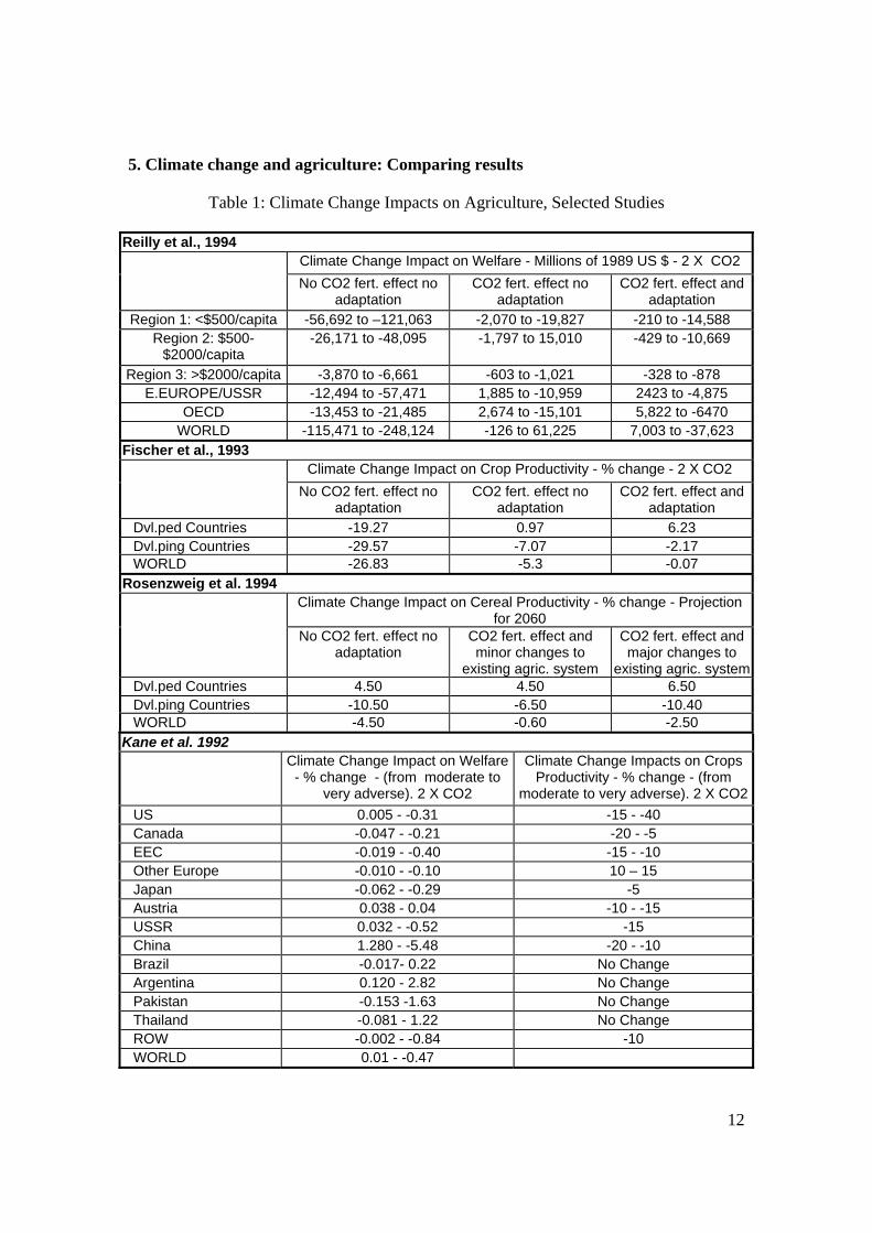
5. Climate change and agriculture: Comparing results

Table 1: Climate Change Impacts on Agriculture, Selected Studies

Reilly et al., 1994 Climate Change Impact on Welfare - Millions of 1989 US $ - 2 X CO2 No CO2 fert. effect no

adaptation CO2 fert. effect no

adaptation CO2 fert. effect and

adaptation Region 1: <$500/capita -56,692 to –121,063 -2,070 to -19,827 -210 to -14,588

Region 2: $500-$2000/capita

-26,171 to -48,095 -1,797 to 15,010 -429 to -10,669

Region 3: >$2000/capita -3,870 to -6,661 -603 to -1,021 -328 to -878 E.EUROPE/USSR -12,494 to -57,471 1,885 to -10,959 2423 to -4,875

OECD -13,453 to -21,485 2,674 to -15,101 5,822 to -6470 WORLD -115,471 to -248,124 -126 to 61,225 7,003 to -37,623

Fischer et al., 1993 Climate Change Impact on Crop Productivity - % change - 2 X CO2

No CO2 fert. effect no adaptation

CO2 fert. effect no adaptation

CO2 fert. effect and adaptation

Dvl.ped Countries -19.27 0.97 6.23 Dvl.ping Countries -29.57 -7.07 -2.17 WORLD -26.83 -5.3 -0.07

Rosenzweig et al. 1994 Climate Change Impact on Cereal Productivity - % change - Projection

for 2060

No CO2 fert. effect no adaptation

CO2 fert. effect and minor changes to

existing agric. system

CO2 fert. effect and major changes to

existing agric. systemDvl.ped Countries 4.50 4.50 6.50 Dvl.ping Countries -10.50 -6.50 -10.40 WORLD -4.50 -0.60 -2.50

Kane et al. 1992 Climate Change Impact on Welfare

- % change - (from moderate to very adverse). 2 X CO2

Climate Change Impacts on Crops Productivity - % change - (from

moderate to very adverse). 2 X CO2US 0.005 - -0.31 -15 - -40 Canada -0.047 - -0.21 -20 - -5 EEC -0.019 - -0.40 -15 - -10 Other Europe -0.010 - -0.10 10 – 15 Japan -0.062 - -0.29 -5 Austria 0.038 - 0.04 -10 - -15 USSR 0.032 - -0.52 -15 China 1.280 - -5.48 -20 - -10 Brazil -0.017- 0.22 No Change Argentina 0.120 - 2.82 No Change Pakistan -0.153 -1.63 No Change Thailand -0.081 - 1.22 No Change ROW -0.002 - -0.84 -10 WORLD 0.01 - -0.47

13

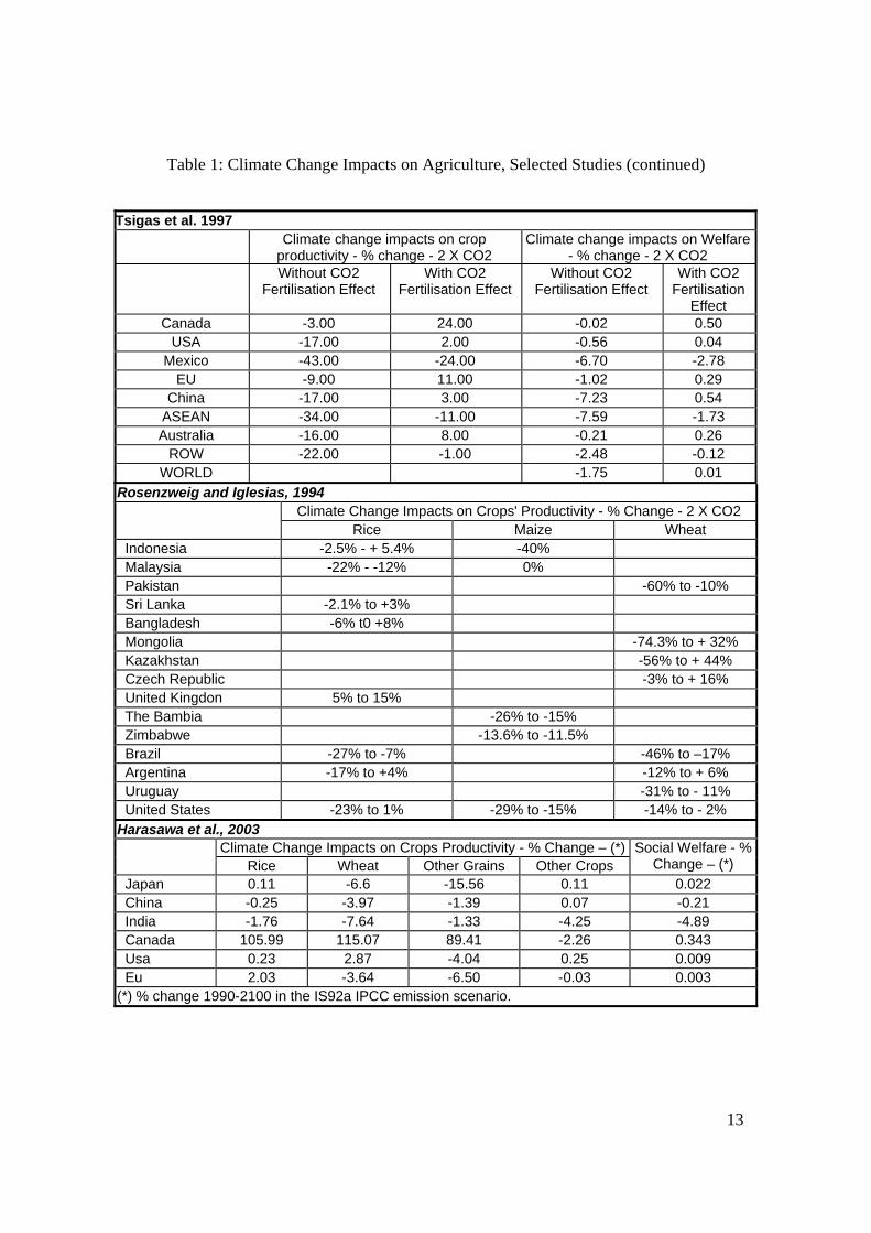
Table 1: Climate Change Impacts on Agriculture, Selected Studies (continued)

Tsigas et al. 1997 Climate change impacts on crop

productivity - % change - 2 X CO2 Climate change impacts on Welfare

- % change - 2 X CO2 Without CO2

Fertilisation Effect With CO2

Fertilisation Effect Without CO2

Fertilisation Effect With CO2

Fertilisation Effect

Canada -3.00 24.00 -0.02 0.50 USA -17.00 2.00 -0.56 0.04

Mexico -43.00 -24.00 -6.70 -2.78 EU -9.00 11.00 -1.02 0.29

China -17.00 3.00 -7.23 0.54 ASEAN -34.00 -11.00 -7.59 -1.73 Australia -16.00 8.00 -0.21 0.26

ROW -22.00 -1.00 -2.48 -0.12 WORLD -1.75 0.01

Rosenzweig and Iglesias, 1994 Climate Change Impacts on Crops' Productivity - % Change - 2 X CO2

Rice Maize Wheat Indonesia -2.5% - + 5.4% -40% Malaysia -22% - -12% 0% Pakistan -60% to -10% Sri Lanka -2.1% to +3% Bangladesh -6% t0 +8% Mongolia -74.3% to + 32% Kazakhstan -56% to + 44% Czech Republic -3% to + 16% United Kingdon 5% to 15% The Bambia -26% to -15% Zimbabwe -13.6% to -11.5% Brazil -27% to -7% -46% to –17% Argentina -17% to +4% -12% to + 6% Uruguay -31% to - 11% United States -23% to 1% -29% to -15% -14% to - 2%

Harasawa et al., 2003 Climate Change Impacts on Crops Productivity - % Change – (*) Rice Wheat Other Grains Other Crops

Social Welfare - % Change – (*)

Japan 0.11 -6.6 -15.56 0.11 0.022 China -0.25 -3.97 -1.39 0.07 -0.21 India -1.76 -7.64 -1.33 -4.25 -4.89 Canada 105.99 115.07 89.41 -2.26 0.343 Usa 0.23 2.87 -4.04 0.25 0.009 Eu 2.03 -3.64 -6.50 -0.03 0.003

(*) % change 1990-2100 in the IS92a IPCC emission scenario.

14

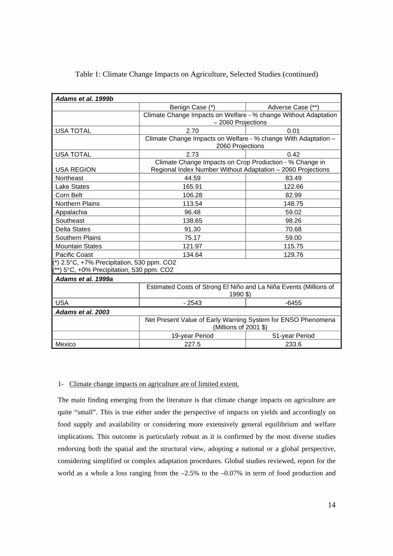
Table 1: Climate Change Impacts on Agriculture, Selected Studies (continued)

Adams et al. 1999b Benign Case (*) Adverse Case (**)

Climate Change Impacts on Welfare - % change Without Adaptation

– 2060 Projections USA TOTAL 2.70 0.01

Climate Change Impacts on Welfare - % change With Adaptation –

2060 Projections USA TOTAL 2.73 0.42

USA REGION Climate Change Impacts on Crop Production - % Change in

Regional Index Number Without Adaptation – 2060 Projections Northeast 44.59 83.49 Lake States 165.91 122.66 Corn Belt 106.28 82.99 Northern Plains 113.54 148.75 Appalachia 96.48 59.02 Southeast 138.65 98.26 Delta States 91.30 70.68 Southern Plains 75.17 59.00 Mountain States 121.97 115.75 Pacific Coast 134.64 129.76

(*) 2.5°C, +7% Precipitation, 530 ppm. CO2 (**) 5°C, +0% Precipitation, 530 ppm. CO2 Adams et al. 1999a

Estimated Costs of Strong El Niño and La Niña Events (Millions of

1990 $) USA - 2543 -6455 Adams et al. 2003

Net Present Value of Early Warning System for ENSO Phenomena

(Millions of 2001 $) 19-year Period 51-year Period Mexico 227.5 233.6

1- Climate change impacts on agriculture are of limited extent.

The main finding emerging from the literature is that climate change impacts on agriculture are

quite “small”. This is true either under the perspective of impacts on yields and accordingly on

food supply and availability or considering more extensively general equilibrium and welfare

implications. This outcome is particularly robust as it is confirmed by the most diverse studies

endorsing both the spatial and the structural view, adopting a national or a global perspective,

considering simplified or complex adaptation procedures. Global studies reviewed, report for the

world as a whole a loss ranging from the –2.5% to the –0.07% in term of food production and

15

ranging from the –0.047% to the 0.01% in term of welfare in case of a doubling CO2

concentration. In regional studies, welfare changes range between the –5.48% and the +2.73% .

It is interesting to note that in general national and partial equilibrium studies report higher

impacts respect to global, general equilibrium studies. As said this confirms the role of

intersectoral and international substitution processes as smoothers. There is however an additional

subtler reason for that: a general equilibrium approach naturally takes into account the welfare of

all the agents within the economic system, and usually losses to one agents turn out to be gains

for another. Typical example is a decrease in consumers’ surplus that is automatically balanced

by the increase in producers’. The net effect is thus reduced.

2- Crucial Role of Adaptation.

It is particularly important to highlight that the limited influence of climate change on agriculture

is mainly due to natural or human adaptation mechanisms. In general strong negative impacts

highlighted by exercises neglecting adaptation turn into much smaller losses or even slight gains

when proper adaptation options are modeled. Interestingly, when it is explicitly taken into

account (see e.g. Reilly et al. 1994; Fischer et al. 1993, Rosenzweigh et al. 1994), the fertilization

effect due to the increased CO2 concentration - that can be considered as an autonomous natural

adaptation process – contributes more to damage reduction than human adaptation. All the studies

confirm in any case the fundamental role of economic adaptation in smoothing adverse climatic

effects.

It is worth to stress here the uncertainty surrounding the modeling of CO2 fertilization effect and

especially of human adaptation options. There are various views about adaptation. Scientists

disagree whether the rate of change of climate and the required adaptations would add

significantly to the disruption that farming will experience form future changes in economic

conditions, technology and resource availabilities (see e.g. Kane and Reilly, 1993; Reilly 1994).

Indeed there are many questions still puzzling regarding to adaptation. For example: how can

agriculture adjust? Rapidly and autonomously, slowly and only with careful guidance? Is there

little scope for adjustment? Does response of the system require planning by farmers specifically

taking into account climate change, and if so what is their capability to detect change and respond

(Reilly, 1999)?

This is an important qualification of the highlighted results. Should adaptation be less effective,

strong adverse consequences of climate change on agricultural production and welfare cannot be

excluded.

16

3- Uneven Distribution of Effects

Agricultural sectors in different regions are likely to be affected and to respond differently to

climate change. In particular results highlight a higher vulnerability of the developing world. On

the one hand this is due to a purely physical fact: the latitude where most part of developing

countries are located. Though employing different methods and scenarios, most studies (see e.g.

Rosenzweig, et al. 1994, Kane et al. 1992, Darwin et al., 1995) generally support the conclusion

that low latitude yields will fall and middle and northern latitude yields will rise with a doubling

of CO2 levels.

On the other hand this is related to their lower capacity to adapt2.

Again, negative impacts are not “big”, but this outcome needs to be carefully qualified: apart

from uncertainties, many developing countries are already experiencing severe risk of hunger and

malnutrition problems. Accordingly even a slight worsening of an already dramatic situation is a

worrying eventuality.

4 – Role of Extreme Events

When climate change is considered only as a variation in average conditions, impacts on

agriculture can be positive and negative. They become unambiguously negative when extreme

events, representing changes in extreme conditions, are taken into account (Adams et al., 1998;

Solow et al., 1998, Chen et al., 2000). Also agriculture reflects this typical characterization of the

relationship between climate change and adaptation: average change is slow and usually falls

within the “coping range” of systems, extreme change is abrupt and often outside this coping

range.

6. The modeling exercise

As an introduction of the modeling exercise performed, we firstly describe the approach used and

place it in the stream of the reviewed literature.

6.1. The modeling approach.

Our investigation is an integrated assessment exercise, conducted at the world level, coupling

with the so-called “soft-link” approach a GCM, an agricultural sub-model and an economic

model. The GCM used is a reduced-form of the Schneider-Thompson GCM: starting from CO2

17

emissions, it provides information on the expected increase in average world temperature and

CO2 concentration in the atmosphere. This average data is then disaggregated into 22 geo-

climatic zones following Giorgi and Mearns (2002) and fed into a crop productivity change

module. This module (Tol, 2004) extrapolates changes in yields respect to a given scenario of

temperature increase. It is based on data from Rosenzweig and Hillel, 1998 which report detailed

results from an internally consistent set of crop modeling studies for 12 world regions and 6

crops’ varieties. The role of CO2 fertilization effect is explicitly taken into account. Finally

changes in yields are used as input in the global economic model in order to assess the systemic

general equilibrium effects.

To do this, we made an unconventional use of a standard multi-country world CGE model: the

GTAP model (Hertel, 1996), in the version modified by Burniaux and Truong (2002), and

subsequently extended by ourselves.

In a first step, we derived benchmark data-sets for the world economy “without climate change”

at some selected future years (2010, 2030, 2050), using the methodology described in Dixon and

Rimmer (2002). This entails inserting, in the model calibration data, forecasted values for some

key economic variables, to identify a hypothetical general equilibrium state in the future.

Since we are working on the medium-long term, we focused primarily on the supply side:

forecasted changes in the national endowments of labour, capital, land, natural resources, as well

as variations in factor-specific and multi-factor productivity.

We obtained estimates of the regional labour and capital stocks by running the G-Cubed model

(McKibbin and Wilcoxen, 1998) and of land endowments and agricultural land productivity from

the IMAGE model version 2.2 (IMAGE Team, 2001). We ran this model by adopting the most

conservative scenario about the climate (IPCC B1), implying minimal temperature changes.

In the second step we imposed over these benchmark equilibria the climate change shock on

agriculture that we model as a change in the productivity of land devoted to the production of the

different crops in the different regions.

Tsigas et al. 1997, perform a similar exercise measuring general equilibrium effect of climate

change in agriculture using the GTAP model. The basic differences between their and our

approach are: firstly the climate scenario, they refer to a doubling of CO2, while we project

directly the temperature increase consistent with the emissions from the economic model;

2 Lower capacity does not mean lower knowledge, skill or ability. Rather it refers to the usually lower amount of resources available for adaptation options or to stronger technological or market constraints to

18

secondly the economic benchmark, they use the model calibrated in 1997, while as said, we

pseudo-calibrated the model in 2050; thirdly the economic shocks, they implemented climate

change as a Hicks neutral technical change in the crop sectors in each region, that is productivity

changes affect uniformly all the production factors used by the agricultural industries while, in

our case climate change intervenes, we believe more realistically, only on land-productivity-

augmenting technical change.

This exercise suffers also from some major limitations. We mention the following:

- firstly an analysis at the world level requires heroic simplifications and generalizations of

both climatic conditions and crop responses. A very narrow number of observations is used to

provide information on vast areas inducing an unrealistic uniformity,

- secondly - apart from temperature and CO2 fertilization effects - other important impacts of

climate change on agriculture are missing, primarily interrelations with water availability and

with livestock,

- thirdly adaptation at the farm level is partly disregarded especially decisions on cultivation

timing as the exercise is purely static. Moreover there is not a land use model defining the

optimal allocation of land among competing alternatives; land is a production factor used

only by the agricultural sector and not for instance by the residential or the industrial sectors,

as a consequence also the mechanism governing the decision on cultivation location results

highly simplified,

- finally the exercise concentrates only on few kinds of cereal crops.

Nonetheless, the exercise is particularly useful in highlighting substitution mechanisms and

transmission channels within and between economic systems. It allows to represent and

disentangle those adaptation mechanisms at work in the modern economies that can amplify or

smooth an initial shock and produce a final effect largely different from the original stimulus.

This crucial role of autonomous national and international socioeconomic adaptation is the matter

of the next subsection.

the adoption of adaptation opportunities in developing countries respect to developed economies.

19

6.2. Results and comments.

In what follows we are reporting results for 2050 when, according to our calculations,

temperature is expected to increase 0.93°C respect to year 2000. Results for the other benchmark

years are qualitatively similar.

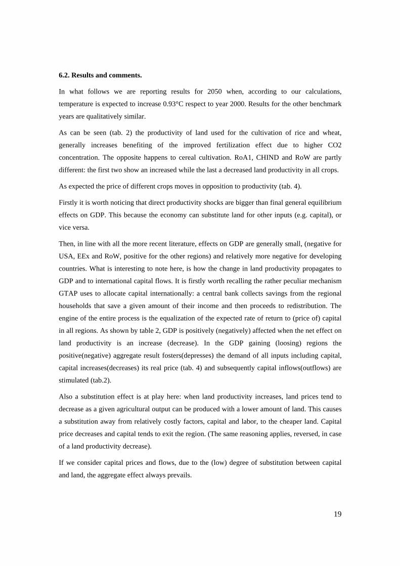
As can be seen (tab. 2) the productivity of land used for the cultivation of rice and wheat,

generally increases benefiting of the improved fertilization effect due to higher CO2

concentration. The opposite happens to cereal cultivation. RoA1, CHIND and RoW are partly

different: the first two show an increased while the last a decreased land productivity in all crops.

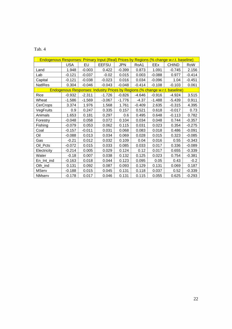
As expected the price of different crops moves in opposition to productivity (tab. 4).

Firstly it is worth noticing that direct productivity shocks are bigger than final general equilibrium

effects on GDP. This because the economy can substitute land for other inputs (e.g. capital), or

vice versa.

Then, in line with all the more recent literature, effects on GDP are generally small, (negative for

USA, EEx and RoW, positive for the other regions) and relatively more negative for developing

countries. What is interesting to note here, is how the change in land productivity propagates to

GDP and to international capital flows. It is firstly worth recalling the rather peculiar mechanism

GTAP uses to allocate capital internationally: a central bank collects savings from the regional

households that save a given amount of their income and then proceeds to redistribution. The

engine of the entire process is the equalization of the expected rate of return to (price of) capital

in all regions. As shown by table 2, GDP is positively (negatively) affected when the net effect on

land productivity is an increase (decrease). In the GDP gaining (loosing) regions the

positive(negative) aggregate result fosters(depresses) the demand of all inputs including capital,

capital increases(decreases) its real price (tab. 4) and subsequently capital inflows(outflows) are

stimulated (tab.2).

Also a substitution effect is at play here: when land productivity increases, land prices tend to

decrease as a given agricultural output can be produced with a lower amount of land. This causes

a substitution away from relatively costly factors, capital and labor, to the cheaper land. Capital

price decreases and capital tends to exit the region. (The same reasoning applies, reversed, in case

of a land productivity decrease).

If we consider capital prices and flows, due to the (low) degree of substitution between capital

and land, the aggregate effect always prevails.

20

Nevertheless this is not generally true considering the land price where the productivity effects

dominate the aggregate effect. An example particularly clear is CHIND: here land productivity

unambiguously increases with a positive effect on GDP, but land price decreases.

Note also that generally terms of trade effects act as smoothers: a relative decrease in GDP

induces a shift toward domestic goods by domestic and foreign consumers attracted by decreasing

prices. This decreases the price of imports and increases the price of exports. Again this is not

always the case. In three regions terms of trade effects amplify rather than smooth the GDP result:

USA, where changes in terms of trade strengthen the negative performance of production and

JPN and CHIND where they reinforce the positive one.

The interplay between terms of trade and capital flows explains also the different sign that

sometimes is observable in the household utility index respect to GDP.

Finally tab. 3 reports industrial production. In general positive GDP and productivity changes

translate in similar changes in production level, particularly of agricultural industries.

21

Tab. 2

Exogenous Shocks on Land Productivity in Different

Agricultural Industries (% change w.r.t. baseline)

Endogenous Responses (% change w.r.t. baseline)

Rice Wheat Cereal

Crops GDP Private Utility Index

Co2 Emissions

Terms of

Trade

Internat. Capital Flows

USA 1.214 1.497 -1.702 -0.023 -0.047 -0.056 -0.183 -0.152 EU 1.811 1.046 -1.134 0.006 -0.005 -0.004 -0.048 0.019 EEFSU 1.856 3.641 -0.822 0.011 0.008 0.001 -0.016 0.037 JPN 0.973 0.399 -1.999 0.004 0.012 0.035 0.023 0.082 RoA1 6.624 8.993 3.619 0.067 0.046 0.032 -0.080 0.1 EEx 1.349 2.063 -1.659 -0.013 0.047 0.010 0.214 -0.002 CHIND 3.962 5.068 0.870 0.212 0.215 0.012 0.095 0.98 RoW -1.791 -1.599 -4.891 -0.126 -0.099 -0.175 0.076 -0.35

Tab. 3

Endogenous Responses: Industry Output by Region (% change w.r.t. baseline) USA EU EEFSU JPN RoA1 EEx CHIND RoW Rice -0.581 -0.498 0.045 -0.086 1.867 -0.015 0.461 -0.505 Wheat -1.025 -0.507 0.513 -3.835 5.851 -0.94 0.715 -2.604 CerCrops -0.523 0.867 0.794 0.511 5.304 0.228 1.7 -3.335 VegFruits -0.386 0.379 0.129 0.206 0.08 -0.111 0.352 -0.355 Animals -0.348 0.112 0.096 0.024 0.182 -0.077 0.4 -0.435 Forestry -0.011 0.023 0.023 -0.022 -0.057 0.022 -0.082 0.01 Fishing 0.126 -0.033 0.017 0.004 -0.11 -0.01 0.082 0.032 Coal 0.05 -0.021 -0.012 -0.127 -0.079 -0.008 -0.153 0.194 Oil 0.08 0.005 -0.003 -0.079 -0.071 -0.004 -0.223 0.205 Gas 0.089 0.018 -0.016 -0.053 -0.191 -0.012 -0.666 0.438 Oil_Pcts -0.077 -0.006 0.015 0.01 0.078 -0.014 0.162 -0.04 Electricity 0.02 -0.006 -0.013 -0.012 -0.135 0.002 -0.051 0.094 Water 0.004 0.003 0.006 -0.008 0.016 0.035 -0.037 0.008 En_Int_ind 0.145 -0.027 -0.042 -0.094 -0.276 -0.076 -0.332 0.257 Oth_ind -0.165 0.027 0.032 0.058 -0.072 -0.054 0.284 -0.345 MServ 0.015 -0.012 -0.012 -0.002 -0.018 0.007 0.082 0.085 NMserv 0.004 -0.004 0.005 -0.008 0.022 0.034 -0.076 0.017

22

Tab. 4

Endogenous Responses: Primary Input (Real) Prices by Regions (% change w.r.t. baseline) USA EU EEFSU JPN RoA1 EEx CHIND RoW Land 1.948 -0.003 0.422 -0.399 0.873 1.091 -0.745 2.156Lab -0.121 -0.037 -0.02 0.015 0.003 -0.088 0.977 -0.414Capital -0.121 -0.038 -0.023 0.016 0.034 -0.096 1.04 -0.451NatlRes 0.304 -0.046 -0.043 -0.048 -0.414 -0.108 -0.103 0.061

Endogenous Responses: Industry Prices by Regions (% change w.r.t. baseline) Rice -0.932 -2.311 -1.726 -0.826 -4.646 -0.916 -4.924 3.515Wheat -1.586 -1.569 -3.067 -1.776 -4.37 -1.488 -5.439 0.911CerCrops 3.374 1.976 1.568 1.761 -0.409 2.635 -0.315 4.395VegFruits 0.9 0.247 0.335 0.157 0.521 0.618 -0.017 0.73Animals 1.653 0.181 0.297 0.6 0.495 0.648 -0.113 0.782Forestry -0.048 0.058 0.072 0.104 0.034 0.048 0.744 -0.357Fishing -0.079 0.053 0.062 0.115 0.031 0.023 0.354 -0.275Coal -0.157 -0.011 0.031 0.068 0.083 0.018 0.486 -0.091Oil -0.088 0.013 0.034 0.069 0.028 0.015 0.323 -0.085Gas -0.21 0.012 0.032 0.109 0.04 0.016 0.55 -0.343Oil_Pcts -0.072 0.015 0.033 0.085 0.033 0.017 0.336 -0.089Electricity -0.214 0.005 0.029 0.124 0.12 0.017 0.655 -0.339Water -0.18 0.007 0.038 0.132 0.125 0.023 0.754 -0.381En_Int_ind -0.163 0.018 0.044 0.123 0.095 0.05 0.43 -0.2Oth_ind 0.131 0.092 0.087 0.093 0.129 0.131 0.069 0.187MServ -0.188 0.015 0.045 0.131 0.118 0.037 0.52 -0.339NMserv -0.178 0.017 0.046 0.131 0.115 0.055 0.625 -0.293

23

7. Conclusions

In this paper we offered a survey of the various approaches used to describe, model and measure

the complex relationships between climate change and agriculture. The main message that can be

grasped from the relevant literature is that climatic, agricultural and economic information need

to be consistently melted in order to provide a reliable and sound impact assessment analysis in

this field. This is witnessed by the constant effort to expand the comprehensiveness of the

investigation that has recently led to the construction of large modeling frameworks coupling

global circulation models, crop growth models, land use models and economic, usually general

equilibrium, models. A robust finding of all these modeling efforts is that climate change impact

on food supply and on welfare are of limited extent. Nevertheless this outcome is largely

determined by the working of socio-economic autonomous and planned adaptation processes,

whose real costs and potential in limiting adverse consequences from climate change are highly

controversial and uncertain. Another robust result is that, notwithstanding adaptation, agricultural

sectors in the developing world will be adversely affected with negative consequences either in

terms of food availability or of welfare. Considering the already dramatic situation faced by many

developing countries even “small” worsening can lead to serious threats to their socio-economic

development. This also raises the crucial issue of proper re-distributional policies from developed

to developing countries.

Finally we proposed an integrated assessment exercise to evaluate climate change impact on

agriculture. As it is standard to the approach we coupled a global circulation model, with a crop-

growth model, with an economic model. Original to our approach is the determination of the

climatic scenario, endogenously produced by the economic model and the benchmarking of the

economic model itself, reproducing a hypothetical world economic system in 2010, 2030 and

2050. The results we get are in line with the existing literature confirming both the limited impact

of climate change on agricultural sectors, largely determined by the smoothing effect of economic

adaptation, but also the relative higher penalization of the developing world.

Acknowledgements

We had useful discussions about the topics of this paper with Roberto Roson, Richard Tol, Katrin

Rehdanz, Kerstin Ronneberger, Filippo Giorgi, Marzio Galeotti, Carlo Carraro, Hom Pant, Guy

24

Jakeman, Huey Lin Lee and Luca Criscuolo. The Ecological and Environmental Economics

programme at ICTP-Trieste provided welcome financial support.

25

References

Adams, R. M. (1999), 'On the Search for the Correct Economic Assessment Method', Climatic Change, 41 (3-4), 363-370.

Adams, R. M., Bryant, K. J., McCarl, B. A., Legler, D.M, O’Brian, J., Solow, A and R. Weiher (1995b) 'Value of Improved Long-Range Weather Information, ' Contemporary Economic Policy, XIII, 10-19.

Adams, R. M., Chen, C.-C., McCarl, B. A., and Weiher, R. F. (1999), 'The Economic Consequencs of ENSO Events for Agriculture', Climate Research, 13, 165-172.

Adams, R. M., Chen, C.-C., McCarl, B. A., and Schimmelpfenning, D.E. (2000), ' Climate Variablility and Climate change: Implications for Agriculture. In The Long Term Economics of Climate Change, ' Volume 3, Advances in the Econmics of Environmental Resources. Hall, D and Howarth, R. Eds. Elsevier Science Publisher, New York, NY.

Adams, R. M., Fleming, R. A., Chang, C. C., McCarl, B. A., and Rosenzweig, C. (1995a), 'A Reassessment of the Economic Effects of Global Climate Change on U.S. Agriculture', Climatic Change, 30, 147-167.

Adams, R. M., Glyer, J.D., McCarl, B. A., and Dudek, D.J. (1988), ' The Implications of Global Change for Western Agriculture, ' Western Journal of Agriculture Economics, 13, 348-356.

Adams, R. M., Houston, L. L., McCarl, B. A., Tiscareno, L.M, Matus, G.J. and R. Weiher (2003), 'The Benefits to MexicanAgriculture of an ENSO Early Warning System, ' Agricultural and Forest Meteorology, 115, 183-194.

Adams, R. M., Hurd, B.H. and J. Reilly (2001), 'Impacts on the US Agricultural Sector', PEW report Climate Change: Science, Strategies and Solutions , 47-64.

Adams, R. M., McCarl, B. A., Segerson, K., Rosenzweig, C., Bryant, K. J., Dixon, B. L., Conner, R., Evenson, R. E., & Ojima, D. (1999), ' The Economic Effects of Climate Change on U.S. Agriculture, ' in The Impact of Climate Change on the United States Economy, R. O. Mendelsohn & J. E. Neumann, eds. (eds.), Cambridge University Press, Cambridge, pp. 18-54.

Adams, R.M., Rosenzweig, C., Peart, R.M., Ritchie, J.T., McCarl, B.A., Glyer, J.D., Curry, R.B., Jones, J.W., Boote, K.J., and Allen Jr. L.H. (1990) , 'Global Climate Change and U.S. Agriculture, ' Nature 345: 219-224.

26

Arthur, L. (1988), 'The Greenhouse Effect and the Canadian Prairies, ' in G. Johnston, D. Freshwater and P. Favero, eds., Natural Resource and Environmental Policy Issues, Boulder, CO: Westview, pp. 233-52.

Bosello, F., Lazzarin, M., Roson, R., and Tol, R.S.J. (2004), 'Economy-Wide Estimates of the Implications of Climate Change: Sea-Level Rise,' FEEM working paper forthcoming.

Burniaux J-M., Truong, T.P., (2002) GTAP-E: An Energy-Environmental Version of the GTAP Model, GTAP Technical Paper n.16 (www.gtap.org).

Butt, T.A. (2002), ' The Economic and Food Security Implications of Population, Climate Change, and Technology – A Case Study For Mali,' unpublished PhD Dissertation, Department of Agricultural Economics, Texas A&M University, College Station, TX.

Butt, T.A., McCarl, B., Angerer, J., Dyke, P., Kim, M., Kaitho, R. and J. Smith (2004), 'Agricultural Climate Change Impact, General Concerns and Findings from Mali, Kenya, Uganda and Senegal, ' Presented at the USAID SANREM CRSP Sustainable Natural Resource Management Accomplishment Workshop. Washington D.C., June 15, 2004.

Chen, C.C., B.A. McCarl, and D. Schimmelpfennig (2000), 'Yield Variability as Influenced by Climate: A Statistical Investigation, ' report under USGCRP Assessment http://ageco.tamu.edu/faculty/mccarl/climchg.html .

Criscuolo, L., Knorr, W. and E. Ceotto (2003), 'Integrated Ecosystem and Crop Modelling for Global Carbon Cycle Assessment', paper presented at the 2nd NCRR International Summer School Grindelwald, Switzerland.

Darwin, R. F. (1997), ' World Agriculture and Climate Change: Current Questions ', World Resource Review, 9 (1), 17-31.

Darwin, R. F. and Tol, R. S. J. (2001), ' Estimates of the Economic Effects of Sea Level Rise, ' Environmental and Resource Economics, 19, 113-129.

Darwin, R. F., Tsigas, M., Lewandrowski, J., & Raneses, A. (1995), World Agriculture and Climate Change - Economic Adaptations, U.S. Department of Agriculture, Washington, D.C., 703.

Darwin, R. F. (1999), 'A FARMer's View of the Ricardian Approach to Measuring Agricultural Effects of Climatic Change, ' Climatic Change, 41 (3-4), 371-411.

Deke, O., Hooss, K. G., Kasten, C., Klepper, G., & Springer, K. 2001, 'Economic Impact of Climate Change: Simulations with a Regionalized Climate-Economy Model, ' Kiel Institute of World Economics, Kiel, 1065.

Dixon, P. and Rimmer, M., (2002) Dynamic General Equilibrium Modeling for Forecasting and Policy, North Holland.

27

Downing, T (1992), 'Climate Change and Vulnerable Places: Global Food Security and Country Studies in Zimbabwe, Kenya, Senegal and Chile,' Research Report No. 1, Environmental Change Unit, University of Oxford, Oxford

Fischer, G., Frohberg, K., Parry, M. L., & Rosenzweig, C. (1993), 'Climate Change and World Food Supply, Demand and Trade,' in Costs, Impacts, and Benefits of CO2 Mitigation, Y. Kaya et al., eds. (eds.), pp. 133-152.

Fischer, G., Frohberg, K., Parry, M. L., & Rosenzweig, C. (1996), 'Impacts of Potential Climate Change on Global and Regional Food Production and Vulnerability, ' in Climate Change and World Food Security, T. E. Downing, ed. (eds.), Springer-Verlag, Berlin, pp. 115-159.

Giorgi, F. and L.O. Mearns (2001), 'Calculation of Average, Uncertainty Range, and Reliability of Regional Climate Changes from AOGCM Simulations via the Reliability Ensemble Averaging (REA) Method,’ Journal of Climate, 15, 1141-1158.

Godwin, D., Ritchie, J., Singh, U. and Hunt, L. (1989). A User’s Guide to CERES-Wheat – V2.10. Muscle Shoals, AL: International Fertilizer Development Center.

Hertel, T.W., (1997) Global Trade Analysis: Modeling and applications, Cambridge University Press.

Hodges, T., Johnson, S.L. and Johnson, B.S. (1992). 'A Modular Structure for Crop Growth Simulation Models: Implemented in the SIMPOTATO Model, ' Agronomy Journal 84: 911-15.

IMAGE (2001), The IMAGE 2.2 Implementation of the SRES Scenarios, RIVM CD-ROM Publication 481508018, Bilthoven, The Netherlands.

IPCC. (1996). Climate Change 1995: The IPCC Second Assessment Report, Volume 2: Scientific-Technical Analyses of Impacts, Adaptations, and Mitigation of Climate Change, Watson, R.T., Zinyowera, M.C. and Moss, R.H.(eds). Cambridge University Press: Cambridge and New York.

Jones, J.W., Boote, K.J., Jagtap, S.S., Hoogenboom, G. and Wilkerson, G.G., (1988). SOYGRO v5.41: Soybean Crop Growth Simulation Model User’s Guide. Florida Agricultural Experiment Station Journal No.8304, University of Florida: IFAS.

Kainuma, M., Matsuoka, Y. and Morita, T. (2003), (eds), Climate Policy Assessment Asia-Pacific Integrated Modeling, Springer-Verlag.

Kane, S., Reilly, J. M., and J. Tobey (1992), 'An Empirical Study of the Economic Effects of Climate Change on World Agriculture', Climatic Change, 21, 17-35.

Lee, H.L. (2004), 'Incorporating Agro-Ecologically Zoned Land Use Data Into the GTAP Framework, ' Paper Presented at the 7Th Annual GTAP Conference on Trade, Poverty and the Environment, Washington D.C., June 17-19.

28

McCarl, B.A., Adams, R.M. and B.H. Hurd (2001), 'Global climate change impacts on agriculture', DRAFT

McKibbin, W.J, Wilcoxen, P.J., (1998), 'The Theoretical and Empirical Structure of the GCubed Model, ' Economic Modelling, vol. 16(1), pp. 123–48.

Mendelsohn, R. O., Nordhaus, W. D., and Shaw, D. (1994), ' The Impact of Global Warming on Agriculture: A Ricardian Analysis', American Economic Review, 84 (4), 753-771.

Mendelsohn, R. O., Nordhaus, W. D., and Shaw, D. (1996), 'Climate Impacts on Aggregate Farm Value: Accounting for Adaptation', Agricultural and Forest Meteorology, 80, 55-66.

Mendelsohn, R. O., Nordhaus, W. D., & Shaw, D. (1999), ' The Impact of Climate Variation on U.S. Agriculture, ' in The Impact of Climate Change on the United States Economy, R. O. Mendelsohn & J. E. Neumann, eds. (eds.), Cambridge University Press, Cambridge, pp. 55-74.

Mooney, S. and Arthur, L., (1990). ' The Impacts of Climate Change on Agriculture in Manitoba, ' Canadian Journal of Agricultural Economics, 38, 685-94.

Neilson, R.P. (1993). 'Vegetation redistribution: A possible biosphere source of CO2 during climatic change, ' Water, Air and Soil Pollution, 70, 659-673.

Neilson, R.P. (1995). 'A model for predicting continental scale vegetation distribution and water balance, ' Ecological Applications, 5, 362-385.

Prinn, R., Jacoby, H., Sokolov, A., C. Wang, X. X., Yang, Z., Eckaus, R., Stone, P., Ellerman, D., Melillo, J., Fitzmaurice, J., Kicklighter, D., Holian, G. and Liu Y. (1999), 'Integrated Global System Model for Climate Policy Assessment: Feedbacks and Sensitivity Studies, ' Climatic Change, 41(3/4), 469-546.

Reilly, J. M. (1994), 'Crops and Climate Change', Nature, 367, 118-119.

Reilly, J. M., Hohmann, N., and Kane, S. (1994), 'Climate Change and Agricultural Trade: Who Benefits, Who Loses?', Global Environmental Change, 4 (1), 24-36.

Reilly, J. M. and Schimmelpfennig, D. (1999), 'Agricultural impact assessment, vulnerability, and the scope for adaptation,' Climatic Change, 43, 745-788.

Ritchie, J.T., Baer, D.B. and Chou, T.W. (1989). Appendix C, 'The Potential Effects of Global Climate Change on the U.S., ' Smith, J.B. and Tirpak, D.A. eds. Washington, dc: U.S. Environmental Protection Agency.

Rosenzweig, M. R. and Binswanger, H. P. (1993). 'Wealth, Weather Risk and the Composition and Profitability of Agricultural Investments,' Economic Journal, 103, 56-78.

29

Rosenzweig, C., and Hillel, D.(1998). ' Climate Change and the Global Harvest: Potential Impacts of the Greenhouse Effect on Agriculture. ' Oxford University Press. New York, N.Y..

Rosenzweig, C. and Iglesias, A. (eds). (1994). Implications of Climate Change for International Agriculture: Crop Modeling Studying. EPA 230-B-94-003.

Rosenzweig, C. and Parry, M. L. (1994). 'Potential Impact of Climate Change on World Food Supply, ' Nature, 367, 133-138.

Schimmelpfennig, D., Lewandrowski, J., Reilly, J. M., Tsigas, M., & Parry, I. W. H. (1996). Agricultural Adaptation to Climate Change -- Issues of Longrun Sustainability, US Department of Agriculture, Washington, D.C., 740.

Schneider, S. (1997), 'Integrated Assessment Modelling of Global Climate Change: Transparent Tools for Policy Making or Opaque Screen Hiding Value-Laden Assumptions? ' Environmental Assessment and Modelling, 2, 229-249.

Solow, A. R., Adams, R. F., Bryant, K. J., Legler, D. M., O'Brien, J. J., McCarl, B. A., Nayda, W., and Weiher, R. F. (1998), 'The Value of Improved ENSO Prediction to U.S. Agriculture', Climatic Change, 39, 47-60.

Tsigas, M.E., Frisvold, G.B. and B. Kuhn (1997), 'Global Climate Change in Agriculture' in Global Trade Analysis: Modeling and Applications. Thomas W. Hertel, editor, Cambridge University Press.

Woodward, F.I., Smith, T.M. and Emanuel, W.R. (1995), 'A global primary productivity and phytogeography model', Global Biogeochemical Cycles 9, 471-490.