Assessing and Testing Hydrokinetic Turbine Performance and ... · Assessing and Testing...
40
Assessing and Testing Hydrokinetic Turbine Performance and Effects on Open Channel Hydrodynamics: An Irrigation Canal Case Study March 2017
Transcript of Assessing and Testing Hydrokinetic Turbine Performance and ... · Assessing and Testing...

Assessing and Testing Hydrokinetic Turbine Performance and Effects on Open Channel Hydrodynamics: An Irrigation Canal Case Study March 2017

(This page intentionally left blank)

Acknowledgments i
AcknowledgmentsThis research was made possible through funding from the Department of Energy’s EERE Office’s Wind and Water Power Technologies Office and the Bureau of Reclamation’s Science and Technology Program. Instream Energy Systems Corp. provided the installation and operation of the HK unit and Reclamation’s Pacific Northwest Region allowed use of the Roza Main Canal and site access. Sandia National Laboratories is a multi- mission laboratory managed and operated by Sandia Corporation, a wholly owned subsidiary of Lockheed Martin Corporation, for the U.S. Department of Energy’s National Nuclear Security Administration under contract DE-AC04-94AL85000.
This report was prepared by:
Budi Gunawan, Water Power Technologies Department, Sandia National Laboratories, Albuquerque, NM, USA
Vincent S. Neary, Water Power Technologies Department, Sandia National Laboratories, Albuquerque, NM, USA
Josh Mortensen, Technical Service Center, Hydraulic Investigations and Laboratory Services, United States Bureau of Reclamation, Denver, CO, USA
Jesse D. Roberts, Water Power Technologies Department, Sandia National Laboratories, Albuquerque, NM, USA

HK IN OPEN CHANNELS REPORT
ii List of Acronyms
List of AcronymsADCP acoustic Doppler current profiler
ADV acoustic Doppler velocimeter
AEP annual energy production
BP battery-powered
CEC current energy converter
CFD Computational Fluid Dynamics
CH conventional hydropower
CS cross-section
D Dimension
DOE Department of Energy
EGL energy grade line
FEMA Federal Emergency Management Agency
FIS flood insurance studies
GPS global positioning system
HGL hydraulic grade line
HK hydrokinetic
MBE multi-beam depth echo sounders
MOU Memorandum of Understanding
MHK marine hydrokinetic
MV moving vessel
NGVD National Geodetic Vertical Datum
RC remote controlled
RTK real-time kinematic
SBE single-beam depth echo sounders
TSR tip-speed ratio
WPTO Water Power Technologies Office

Nomenclature iii
NomenclatureA flow area
b bottom width
Cd turbine drag coefficient
Cp turbine power coefficient
di flow depth normal to flow at section i
D hydraulic depth
Dt instantaneous drag force
E Modulus of Elasticity of the strut
Fr Froude number
g gravitational acceleration
hb energy loss due to turbine blockage
hf friction losses
hm minor losses
ht energy extracted by turbine
L reach length
Ls characteristic length scale of the channel geometry
M bending momentp pressure
P wetted perimeter
PT instantaneous mechanical turbine power
Q flow discharge
r strut diameter R hydraulic radius
Re Reynolds number
So longitudinal channel bed slope
T top width
u, v, w instantaneous streamwise, cross stream and vertical velocities
ui instantaneous velocity components u, v, w
ui’ fluctuating part of ui
ūi mean part of ui or characteristic mean velocity
ū∞ upstream approach velocity at hub height
ūx hub height velocity an x distance downstream of the turbine
ūdef hub height velocity deficit
Ub bulk or section mean velocity
Vi streamwise velocity at section i
Vm velocity component of the velocity head
x, y, z streamwise, cross stream and vertical axes
xi x, y, z axes
y flow depth
yi vertical distance from channel bottom to water surface at section i
zi distance from datum line to channel bottom at section i
Z side slope
αi Coriolis coefficient at section i
ε energy dissipation rate per unit mass
ε_ bending strain
h Kolomogorov microscale
l tip-speed ratio
ν kinematic viscosity
ρ density of water
t instantaneous torque
ω instantaneous turbine angular velocity
cfs cubic feet per second
kW kilowatt
m meter
cm centimeter
m/s meters per second

HK IN OPEN CHANNELS REPORT
iv Executive Summary
Executive SummaryHydrokinetic energy from flowing water in open channels has the potential to support local electricity needs with lower regulatory or capital investment than impounding water with more conventional means. MOU agencies involved in federal hydropower development have identified the need to better understand the opportunities for hydrokinetic (HK) energy development within existing canal systems that may already have integrated hydropower plants. This document provides an overview of the main considerations, tools, and assessment methods, for implementing field tests in an open-channel water system to characterize current energy converter (CEC) device performance and hydrodynamic effects. It describes open channel processes relevant to their HK site and perform pertinent analyses to guide siting and CEC layout design, with the goal of streamlining the evaluation process and reducing the risk of interfering with existing uses of the site. This document outlines key site parameters of interest and effective tools and methods for measurement and analysis with examples drawn from the Roza Main Canal, in Yakima, WA to illustrate a site application.
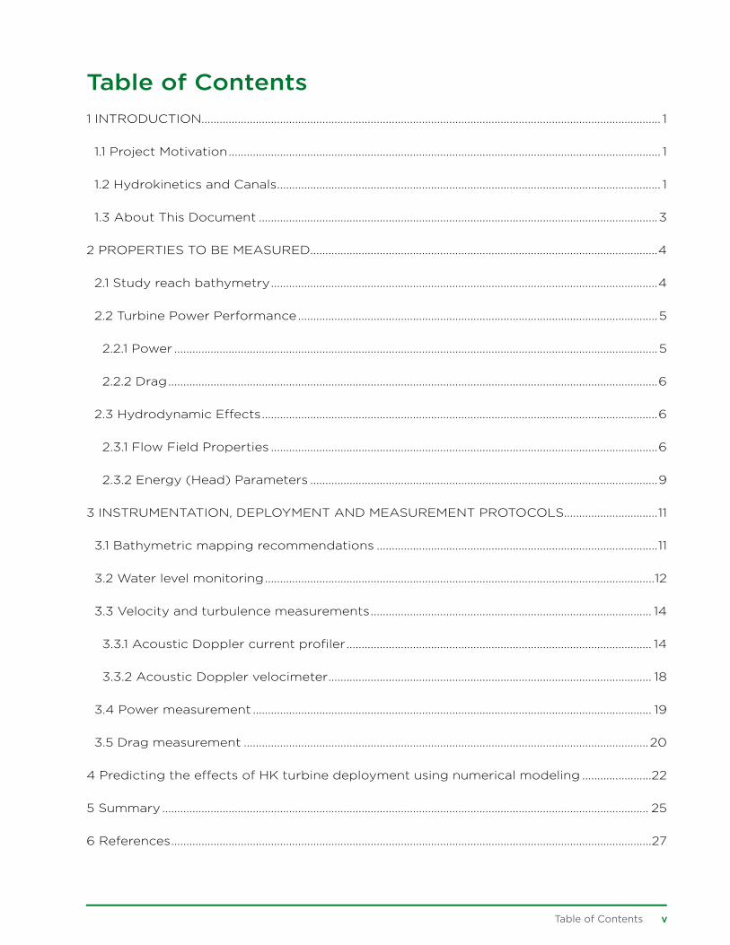
Table of Contents v
Table of Contents1 INTRODUCTION........................................................................................................................................................ 1
1.1 Project Motivation ............................................................................................................................................... 1
1.2 Hydrokinetics and Canals ............................................................................................................................... 1
1.3 About This Document ....................................................................................................................................3
2 PROPERTIES TO BE MEASURED...................................................................................................................4
2.1 Study reach bathymetry ................................................................................................................................4
2.2 Turbine Power Performance .......................................................................................................................5
2.2.1 Power ................................................................................................................................................................5
2.2.2 Drag ..................................................................................................................................................................6
2.3 Hydrodynamic Effects ...................................................................................................................................6
2.3.1 Flow Field Properties ................................................................................................................................6
2.3.2 Energy (Head) Parameters ...................................................................................................................9
3 INSTRUMENTATION, DEPLOYMENT AND MEASUREMENT PROTOCOLS ...............................11
3.1 Bathymetric mapping recommendations .............................................................................................11
3.2 Water level monitoring .................................................................................................................................12
3.3 Velocity and turbulence measurements ............................................................................................. 14
3.3.1 Acoustic Doppler current profiler ..................................................................................................... 14
3.3.2 Acoustic Doppler velocimeter ........................................................................................................... 18
3.4 Power measurement .................................................................................................................................... 19
3.5 Drag measurement ......................................................................................................................................20
4 Predicting the effects of HK turbine deployment using numerical modeling .......................22
5 Summary ................................................................................................................................................................. 25
6 References ...............................................................................................................................................................27

HK IN OPEN CHANNELS REPORT
vi List of Figures
List of FiguresFigure 1. Canal cross-section (left) and profile (right) parameters ..................................................4
Figure 2. Sketch defining flow coordinate system and mean, instantaneous flow profiles,
and flow changes induced by a turbine (Neary et al. 2011). ............................................8
Figure 3. Energy grade line between two locations along a channel in open-channel flow,
adapted from Te Chow (1959). ................................................................................................... 10
Figure 4. The remote control survey boat with real-time kinematic GPS correction. ............11
Figure 5. An example of a coarse bathymetric survey using a single-beam echo sounder
at the Roza Canal site, showing the raw data (left) and the interpolated data
(right).........................................................................................................................................................12
Figure 6. Water level time series at the Roza Canal site, at 50 m and 700 m upstream of
the turbine. ...........................................................................................................................................13
Figure 7. Top left: An example of water level pressure transducer; the length of the
transducer in picture is 15 cm. Top right: Transducer, deployed using a PVC pipe
at the channel’s side wall.
Bottom: angle iron profiles mounted on the channel’s side wall. ................................ 14
Figure 8. Different types of ADCP beam configurations (RDI 2011) ...............................................15
Figure 9. Boat capsize due to highly turbulent flow and uneven water surface
downstream of a turbine. .................................................................................................................15
Figure 10. A cableway deployment with a tensioned tagline (the white line), that is
attached to the ADCP boat. ......................................................................................................... 16
Figure 11. ADCP velocity contours (looking downstream), as shown in the RD Instrument’s
WinRiver software, at four cross-sections at the Roza Canal test site: 50 m
upstream of the turbine, 10 m downstream of the turbine, 20 m downstream of
the turbine, and 30 m downstream of the turbine. The x axis shows the length
of the ADCP travel path while traversing the canal. ..........................................................17
Figure 12. Spatiotemporally-averaged velocity contour (looking downstream), 10 m
downstream of the turbine, at Roza Canal under high tip-speed ratio. Flow
discharge was approximately 55 m3/s. Black scatters in the top figure indicate
the locations of velocity measurements. .................................................................................17
List of Figures and Tables vii
Figure 13. Streamwise velocity contours, interpolated from MV ADCP survey. Left: near-
surface velocities, right: hub-level velocities. The white circle indicates the
locations of the Instream turbine. ............................................................................................. 18
Figure 14. Cable-deployed ADVs (in circles) with sounding weight (Photograph courtesy
of Bob Holmes, USGS, 2010). ....................................................................................................... 19
Figure 15. Sandia’s mobile ADV deployment system for canal measurements. On top is the
schematic of the system and a picture of the unit deployed in the field is shown
on the bottom. .................................................................................................................................... 19
Figure 16. The torque sensor system mounted to the Instream’s turbine shaft at Roza
Canal. The small brown rectangular sensor to the left of the torque sensor
system is a strain gauge used for drag measurements. .................................................20
Figure 17. An example of a battery-powered wireless strain sensor system, for torque or
thrust measurement (www.binsfeld.com). ...........................................................................20
Figure 18. An example of a turbine performance curve for different tip-speed ratios. .......20
Figure 19. Strain gauge mounting location for measuring turbine drag on cross-flow wind
turbine (Griffith et al. 2011). ...........................................................................................................21
Figure 20. Model-predicted velocity contours for Roza Main Canal site (at turbine mid-
span, flow is from top to bottom). The left figure shows the whole simulation
domain, with a turbine positioned near the outflow boundary. The right figure
is the velocity contour at the turbine location. Legend units are in meter/
second. .................................................................................................................................................. 23
Figure 21. Measured and simulated wake velocities at turbine mid-span at Roza Main
Canal, as a function of distance from the turbine. ........................................................... 23
Figure 22. Simulated Energy Grade Lines and Hydraulic Grade Lines (water surface
elevations along the reach) at Roza Main Canal with and without the turbine’s
presence. ............................................................................................................................................... 24
List of TablesTable 1 Recommended measurements for the assessment of potential impacts from open-channel
HK operations. .............................................................................................................................................. 25

(This page intentionally left blank)
Introduction 1
1 INTRODUCTION
1.1 Project MotivationIn 2010, a Memorandum of Understanding (MOU) regarding federal hydropower development in the U.S. was signed by the Department of Energy (Office of Energy Efficiency and Renewable Energy), the Department of the Interior (Bureau of Reclamation), and the Department of the Army (Corps of Engineers), and was later re-signed in 20151. The 2015 Phase II MOU Action Plan developed by the MOU agencies identified the need to better understand the potential for hydrokinetic (HK) energy development within existing canal systems that may already have integrated hydropower plants. Because HK generation of electricity from flowing water in open channels may be less infrastructure intensive than conventional hydropower, that impounds free flowing water, it has the potential to support local electricity needs with lower regulatory or capital investment. This work is specifically aligned with renewable energy development goals of the Department of Energy (DOE) and the Department of the Interior (DOI) by investigating how much excess energy is available for electricity generation via hydrokinetic technologies, while still meeting the design requirements of the existing water supply systems and needs of the water users. As an ancillary benefit of this work, many of the methods and tools developed will be directly transferable to the MHK industry for future potential developments in large rivers, tidal channels, and open ocean currents. This aligns well with the primary goal of the DOE Water Power Technologies Office (WPTO) to efficiently develop and utilize the country’s marine hydrokinetic (MHK) and conventional hydropower (CH) resources.
1.2 Hydrokinetics and CanalsCurrent energy conversion (CEC) technologies are a class of marine and hydrokinetic (MHK) technologies that convert kinetic energy of canal, river, tidal or ocean water currents to generate electricity. Most CEC technologies under development are water turbines, or hydrokinetic (HK) turbines, that are modeled after wind turbines. The two common classes of HK turbines are axial-flow turbines, in which the rotor shaft is oriented parallel to the water current, and cross-flow turbines, in which the rotor shaft is oriented perpendicular to the water current. The shaft of cross-flow turbines can be oriented either vertically or horizontally. Both of these HK turbine classes can be deployed in rivers and canals with additional design work and considerations to maximize energy generation from natural and man-made features.
National MHK resource assessments have been conducted for wave, ocean current, tidal and river sites (EPRI 2011; Yang et al. 2015; Defne et al. 2012; EPRI 2012, respectively) with funding from the DOE. The EPRI 2012 report determined a theoretical resource availability of 1,381 TWh/year from river currents in the U.S., a significant resource. Nearly 72,000 river segments with mean annual flow greater than 1,000 cubic feet per second (cfs) were included in the assessment. The assessment, however, did not include canals and waterways. Therefore, the overall potential for hydrokinetic energy production in these types of water conveyance channels is uncertain. Nevertheless, high current speeds and resource predictability in canals and their general accessibility may be favorable for energy generation through HK technologies.
The US canal system comprises tens of thousands of miles of canals. Existing canals come in a variety of shapes and sizes to meet their primary objective of conveying water to support irrigation, navigation, and hydropower developments. Canals are either earthen (unlined) or lined (often with concrete) to minimize unwanted changes
1 More information on the Federal Hydropower MOU is available at: http://en.openei.org/wiki/Federal_Memorandum_of_Understanding_for_Hydropower
Hydrokinetic energy from flowing water in open channels has the potential to support local electricity needs with lower regulatory or capital investment than impounding water with more conventional means.

HK IN OPEN CHANNELS REPORT
2 Introduction
to canal specifications that may result from scour, vegetation, etc. Those for navigation usually have low current speeds, often well below turbine cut in speeds, and generally do not hold great potential for hydrokinetic development. Many irrigation canals and power canals that feed into or out of hydropower dams display the characteristics needed for HK energy development (i.e. have sufficient current speeds and water depths). In all cases, the development of HK in canals requires strict coordination with existing canal owners to avoid interference with the canal’s primary objective. Each canal type presents unique design challenges and opportunities for HK energy development.
While not all of these canals are suitable for HK energy development, some will have flow speeds, water depths, and other attributes, e.g., proximity to grid connection, favorable for commercial HK energy development. Favorable characteristics for cost-effective HK energy development can include high current speeds (>1.5 m/s) corresponding to high resource; high free-board level (vertical distance between the water surface and top of the channel) to allow greater flexibility of water level variation prior to water exceeding freeboard limits of the canal; and good site access (ability to bring equipment to the canal’s edge). Lined channels are also generally more favorable than unlined channels, as they are more resistive to scour. Channels that do not have protected organisms living in them, will have comparatively, less environmental compliance requirements.
Potential concerns include disrupting water supply operations (by affecting head-discharge conditions at irrigation canal intakes), increasing flood risks (by increasing water levels as a result of blockage and backwater effects), reducing power generation of hydropower plants (by affecting plant inflow, tailwater levels and net head at hydropower dam or discharge), and causing channel instabilities that lead to unfavorable morphological changes. Furthermore, man-made canals are generally designed for a specific purpose and operating regime, such that the design velocities and flow depths are given careful consideration to meet the canals primary objective. HK canal deployments would necessarily change the hydrodynamics of the canal. It is critical to account for these changes to ensure adverse effects, e.g., unwanted sediment deposition (silting), scouring, overtopping, diversion, and reduction in CH energy production, are avoided.
The amount of water conveyed by a canal or a river is variable throughout the year due to, for example, seasonal rainfall and irrigation demands. Therefore, the HK resource in rivers and canals varies seasonally. Adding hydrokinetic turbines to these systems would also change the local/reach hydrodynamics, which if not carefully accounted for could cause unwanted events, such as flooding, silting and scouring. All of these factors should be taken into account in the design, operation, and overall development of hydrokinetics in these resources. Furthermore, there may be opportunities to design new canals to maximize HK potential through features or geometries and also to deploy HK in rivers. For example, unconventional techniques could allow for harvesting energy from rapids, maximizing natural and/or engineered characteristics of rivers and canals.
Feasibility studies for HK energy development must demonstrate that HK operations will not adversely affect canal operations and other stakeholders. A combination of field measurements and numerical modeling can be used for impact assessment of HK projects by evaluating changes to basic
Although resource assessments have been conducted for wave, ocean current, tidal, and river sites, the potential for HK energy production in canals and waterways is uncertain. However, certain canals, including irrigation and power canals, have flow speeds, water depths, and site characteristics that are favorable for commercial HK energy development.
Potential concerns, such as disrupting water supply operations, increased flood risks, reduced power at hydropower plants, unfavorable morphological changes, and seasonal water variability, should be taken into account in the planning, design, and operation of a HK energy project.
Introduction 3
hydrodynamic parameters, such as changes to water surface elevations and velocities at different locations along and across the canal resulting from an HK project.
1.3 About This DocumentThis document is intended as a “how to” manual for conducting hydrokinetic (HK) performance testing in canals and rivers, and assessing the effects of HK device deployment on hydrodynamics. Although this manual provides detailed information based on a single HK case study in a conduit canal with known flow velocity, the methodology presented here is highly applicable to a variety HK design opportunities and infrastructure additions in other types of canals and rivers. This manual is largely written for engineers and researchers who have background knowledge on turbine performance and open channel hydraulic measurement, analysis, and field testing. Other users will benefit from the methods and experience shared in this manual. The methods presented in this manual may not be suitable for all sites, but users are expected to adapt the presented measurement methods, or other methods, for their site and technology specific conditions.
The manual provides information for designing and implementing testing in an open channel system for characterizing device performance and the hydrodynamic effects of single device and array deployments. Chapter 2 outlines the recommended parameters for analyzing device performance and hydrodynamic effects. These parameters include power coefficient, turbine tip-speed ratio, inflow velocity, and water level. Some of the Chapter 2 contents are summarized from the case study manual for river and tidal sites (Neary et al. 2011). Chapter 3 focuses on the types of instrumentation and methods to be used for characterization, including data post-processing methodology. Emphasis is placed upon acoustic-Doppler current profiler (ADCP) and acoustic Doppler velocimeter (ADV) instruments for collecting hydrodynamic measurements, as these instruments represent the most practical and economical tools for use in the MHK industry. Chapter 4 describes the ability of numerical models, of varying fidelity, to predict the hydrodynamic changes induced by HK deployments and how they may be used in conjunction with field measurements.
Much of the insights and materials presented in chapters 3 and 4 are gained from a hydrokinetic turbine case study at the Roza Main Canal, Yakima, WA. The Roza Main Canal is approximately 11 miles long and diverts flow from the Yakima River to the Roza Irrigation District where it supplies water for approximately 72,000 acres of valuable farm land. It typically operates for about 11 months out of the year and shuts down for one month for inspections and maintenance. The 11 mile reach features both lined and unlined sections as well as a bifurcation at the downstream end where a portion of the flow is diverted to a power plant and then returns to the Yakima River. Instream Energy Systems Corp. is currently using the Roza Main Canal site for testing a vertical-axis hydrokinetic turbine. Readers interested in the details of ADV and ADCP measurement and data post processing can refer to the guidance manuals Gunawan and Neary (2011) and Gunawan et al. (2011), which provide detailed methods and protocols for the application of these instruments for MHK reconnaissance, feasibility, design and testing studies .This document provides an overview of the main considerations for an open-channel CEC deployment site and the tools and protocols to help guide the reader through a thorough site and technology assessment. It describes open channel processes relevant to their HK site and perform pertinent analyses to guide siting and CEC layout design, with the goal of streamlining the evaluation process and reducing the risk of interfering with existing uses of the site. This document outlines key site parameters of interest and effective tools and methods for measurement and analysis with examples drawn from the Roza Main Canal, in Yakima, WA to illustrate a site application.
Using the Roza Main Canal in Yakima, WA as a case study, this document provides readers with an overview of key considerations, tools, and protocols to conduct open-channel system site assessments and performance testing.
HK IN OPEN CHANNELS REPORT
4 2 Properties to be Measured
2 PROPERTIES TO BE MEASURED
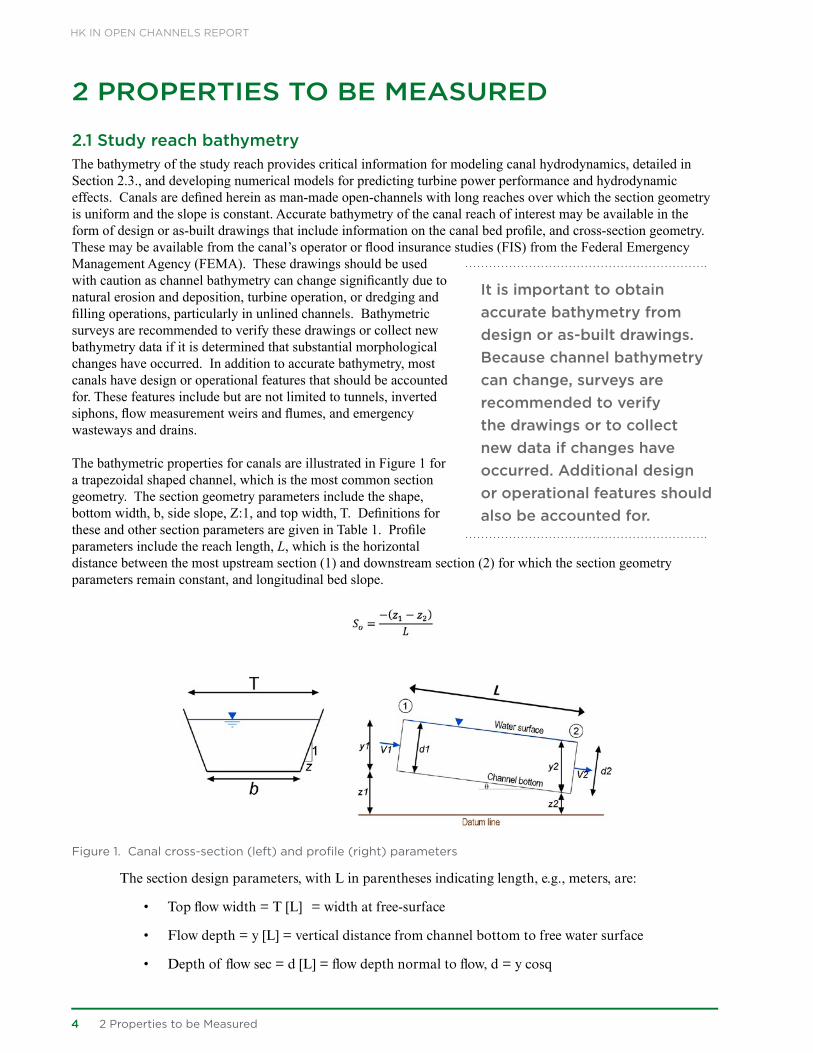
2.1 Study reach bathymetryThe bathymetry of the study reach provides critical information for modeling canal hydrodynamics, detailed in Section 2.3., and developing numerical models for predicting turbine power performance and hydrodynamic effects. Canals are defined herein as man-made open-channels with long reaches over which the section geometry is uniform and the slope is constant. Accurate bathymetry of the canal reach of interest may be available in the form of design or as-built drawings that include information on the canal bed profile, and cross-section geometry. These may be available from the canal’s operator or flood insurance studies (FIS) from the Federal Emergency Management Agency (FEMA). These drawings should be used with caution as channel bathymetry can change significantly due to natural erosion and deposition, turbine operation, or dredging and filling operations, particularly in unlined channels. Bathymetric surveys are recommended to verify these drawings or collect new bathymetry data if it is determined that substantial morphological changes have occurred. In addition to accurate bathymetry, most canals have design or operational features that should be accounted for. These features include but are not limited to tunnels, inverted siphons, flow measurement weirs and flumes, and emergency wasteways and drains.
The bathymetric properties for canals are illustrated in Figure 1 for a trapezoidal shaped channel, which is the most common section geometry. The section geometry parameters include the shape, bottom width, b, side slope, Z:1, and top width, T. Definitions for these and other section parameters are given in Table 1. Profile parameters include the reach length, L, which is the horizontal distance between the most upstream section (1) and downstream section (2) for which the section geometry parameters remain constant, and longitudinal bed slope.
Figure 1. Canal cross-section (left) and profile (right) parameters
The section design parameters, with L in parentheses indicating length, e.g., meters, are:
• Top flow width = T [L] = width at free-surface
• Flow depth = y [L] = vertical distance from channel bottom to free water surface
• Depth of flow sec = d [L] = flow depth normal to flow, d = y cosq
It is important to obtain accurate bathymetry from design or as-built drawings. Because channel bathymetry can change, surveys are recommended to verify the drawings or to collect new data if changes have occurred. Additional design or operational features should also be accounted for.

2 Properties to be Measured 5
• Flow area = A [L2] = cross-sectional area normal to flow direction
• Wetted perimeter = P [L] = length of channel boundary in contact with water
• Hydraulic radius = R [L] = A/P
• Hydraulic depth = D [L] = A/T
2.2 Turbine Power PerformanceTurbine power performance tests typically measure the mechanical power of the turbine, the drag (thrust) force acting on the turbine, and the hydrodynamic force of the approach flow over a range of tip-speed ratios (TSR). The ratio of the mechanical power to the hydrokinetic power of the approach flow, the power coefficient, is a measure of the efficiency of the CEC technology. The ratio of the drag force to the hydrodynamic force of the approach flow is defined as the drag coefficient, which is equivalent to the thrust coefficient when the turbine is stationary (fixed position) because the drag and thrust forces are in balance. These metrics provide essential information that allow CEC technology developers to assess the performance of their turbine technologies relative to other turbine technologies, and to calculate the technical annual energy production (AEP) for hydrokinetic power projects. They are also required data for certifying CEC technologies.
2.2.1 PowerInstantaneous turbine power can be determined from synchronous torque and rotor position measurements (mechanical power). Instantaneous mechanical turbine power, PT , is the product of instantaneous torquet, and instantaneous turbine angular velocity, ω.
The TSR is defined as the ratio of the rotor tip speed to the speed of the approaching flow,
where w is the instantaneous angular velocity. Turbine power coefficient, Cp, can be calculated as,
where A is the turbine’s flow facing area, p is the density of water and u is the instantaneous inflow velocity over the turbine’s flow facing area. The turbine’s flow facing area is the multiple between the rotor diameter and rotor height for vertical axis turbines (essentially a rectangular flow facing area) while an axial flow turbine has a circular flow facing area calculated from the diameter of the turbine only. In the calculation of Cp, the divisor term indicates the theoretical resource availability in the channel, therefore the inflow velocity needs to be measured far enough upstream of the turbine such that turbine drag has little to no effect on the upstream velocity. A distance of three to five turbine diameters is typically sufficient for this purpose (Hill et al. 2014; Hill et al. 2014; Neary et al. 2013).
Note that the term Cp is often used to describe power coefficient derived from the electrical power output instead of mechanical power. The electrical power output is the power generated after taking into account the total efficiency of the system. The total efficiency of the system can include efficiencies of the gearbox, drive train, and generator. Example values of the efficiencies of these components are presented in publications, such as Hagerman et al.
Measuring the mechanical power of the turbine, drag force on the turbine, and hydrodynamic force of the approach flow is essential to assess the performance of turbine technologies and to calculate the annual energy production for HK power projects.

HK IN OPEN CHANNELS REPORT
6 2 Properties to be Measured
2006, which states a range of efficiencies between 95% to 98%. It is therefore always recommended to state the type of power (mechanical or electrical output) used for calculation when reporting a Cp value.
2.2.2 Drag The hydrodynamic force acting on the rotor can be evaluated using the drag coefficient. The turbine drag coefficient, Cd, can be calculated as,
where Dt is instantaneous drag force. The drag coefficient often varies with the TSR.
2.3 Hydrodynamic EffectsAny object placed in moving water will obstruct the flow and introduce a drag force, or drag. Under subcritical flow conditions, this drag will cause water levels to rise upstream of the obstruction (backwater) and drop downstream (drawdown). Hence deployment of HK turbines can alter water levels at various locations along the canal. One important consideration is whether a HK turbine deployment may raise the water levels enough to encroach the canal’s free-board requirement (maximum flow depth relative to top of canal bank) which increases the risk for overtopping. If a threat of overtopping exists, the extent of the affected area needs to be determined to predict damage and assess mitigation options. One of the mitigation options would be to operate the canal below the normal condition, e.g. reducing the flow in the canal, which is likely undesirable. Continuous water level monitoring along the canal and knowledge of canal’s bathymetry are essential to be able to determine if overtopping could occur and its potential extent.
Another important consideration is whether a HK turbine deployment could create sediment deposition or scouring due to modifications to the flow velocities around the turbine. Too low of a velocity can cause sediment deposition, while too high a velocity can cause sediment scouring. The velocity magnitudes at different locations around the turbine should be sufficient enough to keep sediments in suspension without scouring. Permissible velocities vary for channels with different lining materials and other channel parameters. Permissible velocity can be found in the literature, such as a manual developed by the US Army Corps of Engineer (USACE 1994).
2.3.1 Flow Field PropertiesThe flow field within a canal reach is the distribution of the instantaneous streamwise x, cross stream y, and vertical z components of velocity (u, v, w) and pressure p over space and time.These flow field properties are typically time-averaged to reduce the amount of information to a tractable description of the flow field for engineering analysis (Neary et al. 2011). The time-averaged u can also be spatially averaged over the entire section to determine the bulk or section mean velocity Ub. Instantaneous velocities are also important for determining instantaneous loads that contribute strongly to fatigue failure.
2.3.1.1 Bulk Flow and Section Geometry PropertiesBulk flow properties that characterize the flow at a canal cross-section at the time of measurement include the bulk velocity
Continuous water level monitoring and knowledge of the canal’s bathymetry is needed to determine the potential for overtopping. Velocity magnitudes should be sufficient enough to prevent sediment deposition or scouring.

2 Properties to be Measured 7
where Q is the flow discharge in the channel and A is the cross-section area; and section parameters (flow depth, y, top width, T, flow area, A, hydraulic depth D, wetted perimeter P, and hydraulic radius R) which are calculated from field measurements using the equations described in section 2.1. Methods for estimating the flow resistance parameter, Manning’s n, can be found in common references on open-channel hydraulics (e.g., Sturm (2001)). As the channel discharge (flow) was steady at the time of measurements, these bulk flow properties did not vary with time at any given section in the canal reach. However, the flow in the study reach was nonuniform, meaning these properties vary over the length of the channel.
These properties are used to calculate important non-dimensional parameters that indicate the flow state and flow regime, the Reynolds number Re and the Froude number Fr, which are calculated as,
For Re values above about 2,000 - 4,000 inertial forces dominate over viscous forces, creating flow instabilities and turbulence. Only canals with relatively fast moving, therefore, turbulent flow are suitable for HK deployment. The Re value in these canals is typically well over 105. Fr value below one indicates that the celerity or speed of propagation of a small surface wave is greater than the bulk velocity (i.e. gravitational forces dominate over inertia). Most reaches of canals are designed to ensure subcritical flow regimes to reduce the potential for scour. As a result, flow conditions upstream, e.g., velocity and water depth, are influenced by downstream conditions. For example, the placement of a hydrokinetic turbine at a section in a canal causes a local obstruction that increases the water surface elevation. This local rise in the water surface is transmitted upstream, resulting in higher water surfaces, and reduced velocities upstream.
2.3.1.2 Mean (Time-averaged) inflow velocity and velocity deficit
The instantaneous velocity component is decomposed into its time-mean and turbulent fluctuation, 'iii uuu += along its respective axis as illustrated in Figure 2. The instantaneous velocities u, v, w are
defined herein as the streamwise, cross-stream, and vertical velocity components, respectively. The most common means of characterizing a flow field is to measure the statistics of the flow from the mean velocity up through higher order statistics such as the flow skewness and kurtosis. These statistical measures can provide a wealth of information related to the time or space averaged flow, however, they do not provide a measure of the scale and of the instantaneous, unsteady flow structures that may be important in generating unsteady loads, vibration and noise. These unsteady flow structures tend to have smaller spatial scales with higher magnitude fluctuations and local gradients than the time averaged profiles would suggest.
The instantaneous mean inflow velocity, as discussed in section 2.2., is important for determining device performance and loading. Additionally, the mean streamwise velocity deficit is a common metric used to assess the velocity recovery in the wake downstream of a turbine, and to optimize the turbine layout in a turbine farm. The velocity deficit can be defined as
where is the upstream approach velocity at hub height and is the hub height velocity at position x downstream of the turbine.
Inflow velocity measurements are important for determinining device.

HK IN OPEN CHANNELS REPORT
8 2 Properties to be Measured
Figure 2. Sketch defining flow coordinate system and mean, instantaneous flow profiles, and flow changes induced by a turbine (Neary et al. 2011).
2.3.1.3 Turbulence and periodic motion in the flowWhen flows are turbulent, the flow field properties at any given point, for any instant in time, depart from the mean (time-averaged) flow over relatively small space and time scales as illustrated in Figure 2. These time scales can be characterized from small (i.e., Kolmogorov microscale = ) to large (i.e., convective time-scale = ), where ν is the kinematic viscosity, ε is the energy dissipation rate per unit mass, L is a characteristic length scale of the channel geometry (e.g., flow depth) and is a characteristic mean velocity. Turbulent flow is three-dimensional and three-component, and is characterized by a continuous range of flow scales in the form of rotational motion (vortices or eddies). This range of spatial scales in a turbulent flow is dependent on the Reynolds number, Re, where the higher the Reynolds number the broader the range of scales. The smallest scale in a turbulent flow is limited by the fluid viscosity and is estimated by the Kolmogorov (spatial) microscale, η = (ν3/ε)¼, while the largest spatial scale is characterized by the channel bounding geometry, L or a multiple thereof.
The turbulence intensities are dimensionless parameters that describe the level of turbulence within the flow along each spatial direction. Turbulence speeds up the wake velocity recovery, which allows closer spacing between turbines. Turbulence intensities are defined as the root-mean square of the fluctuating velocity component divided by the mean velocity magnitude,
.
; ;
Turbulence occurs in both wall bounded (solid surfaces such as the bed floor) and in free shear flows such as wakes formed behind HK devices, shown in Figure 2. In addition to these turbulent inflow structures, unsteady downstream flow structures, that may be locally turbulent, may exist such as vortical flow structures and unsteady or cyclic flow shedding. The types of vortical flow structure created is dependent on device design and mounting configuration, but may consist of blade tip vortices, tower/bed-floor junction vortices and Karman vortex street associated with flow shedding off of structures. The downstream wake of the device will consist of both large scale (on the order of the rotor plane) and smaller scale flow structures. The large or macro-scale momentum deficit wake of the device may have a rotational flow pattern related to blade rotation and will have characteristic cyclic frequencies associated with the blade passage frequency. The smaller scale structures will consist of individual wakes, vortices and flow unsteadiness as illustrated in Figure 2. Proper characterization of both the inflow and downstream flow features is important in determining overall device performance in single and array deployments. While the mean flow resource directly impacts long term device power output and powering performance, it is the short term unsteady flow characteristics which create unsteady loads on the device components, vibration, and sound generation.
u
u
mean flow profile
Turbulent inflow
Blade & towerWakes
Tip vortices
Flow shedding
Blade Rate: blade passage frequency
Neary et al 2010Junction vortices
z,w
Information on flow turbulence is useful for numerical models to accurately predict wake velocity recovery.

2 Properties to be Measured 9
2.3.2 Energy (Head) ParametersThe section averaged 1D conservation of energy equation is typically applied, along with continuity (conservation of mass) and the conservation of momentum, to model steady open-channel flow hydraulics in canals, and changes in velocity and water depth due to a variety of modifications, including the deployment of instream structures, water diversion, and energy extraction. All terms in the energy equation are normalized by the unit weight of water, which results in energy head in length units [e.g., N-m/N = m]. The total energy head at any given section consists of the sum of the elevation head, z, the piezometric head (water depth), y, and the velocity (kinetic energy) head, aVm2/2g. As the water flows downstream energy losses due to friction, turbulence, and energy extraction are incurred. Due to the nonuniform velocity distribution in a cross-section, the average velocity head does not equal the velocity head of the average velocity,
A correction factor, the Coriolis coefficient, must, therefore, be applied to make the adjustment in the energy equation,
, where
The hydraulic grade line (HGL) is the water surface profile, which is the line drawn through z + y values at all sections along the canal reach. The energy grade line (EGL) is the profile drawn through the total energy at all sections along the canal reach. Methods for determining friction and minor losses are given in standard open channel hydraulics texts (e.g., Sturm 2001).
= Bed elevation at an upstream location, relative to a datum (m)
= Water sdepth upstream (m)
= Coriolis coefficient upstream (-)
= Mean streamwise velocity upstream (m/s)
g = Gravitational acceleration (m/s2)
= Bed elevation at a downstream location, relative to the datum used for (m)
= Water depth downstream (m)
= Coriolis coefficient downstream (-)
= Mean streamwise velocity downstream (m/s)
= Minor losses (m)
= Friction losses (m)
= Energy extracted by turbine (m)
= Energy loss due to turbine blockage (m)

HK IN OPEN CHANNELS REPORT
10 2 Properties to be Measured
Figure 3. Energy grade line between two locations along a channel in open-channel flow, adapted from Te Chow (1959).
The HGL describes the variation in the water surface upstream, and the potential for overtopping the banks and flooding. The EGL, with HGL, describes variation of velocity head and velocity over the channel reach upstream of the turbine. The velocity is an important bulk parameter (section-averaged) that indicates potential for scour or deposition due to hydraulic changes.
3 Instrumentation, Deployment and Measurement Protocols 11
3 INSTRUMENTATION, DEPLOYMENT AND MEASUREMENT PROTOCOLS
3.1 Bathymetric mapping recommendationsBathymetric mapping techniques recommended for a canal site are survey-grade single and multi-beam depth echo sounders (SBE, MBE) coupled to a global positioning system (GPS) with real-time kinematic (RTK) correction. An RTK correction consist of a rover receiver, mounted to the survey boat, and a stationary on-shore base station which provides corrections to the rover receiver to obtain up to centimeter positioning accuracy. The RTK system is a significant upgrade from the common single-receiver differential GPS system that only has decimeter accuracy. The RTK GPS is especially recommended for sites, such as a narrow canal, where positioning errors can adversely affect the study result significantly.
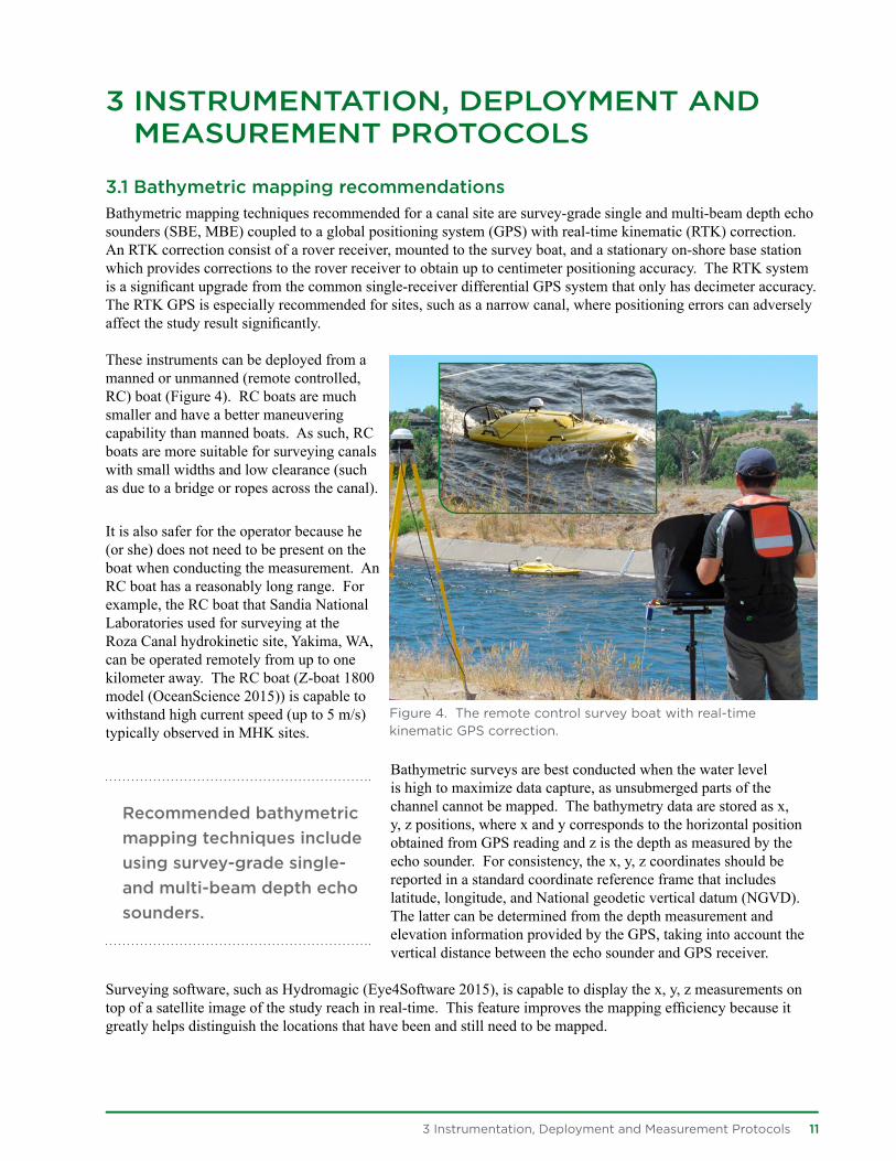
These instruments can be deployed from a manned or unmanned (remote controlled, RC) boat (Figure 4). RC boats are much smaller and have a better maneuvering capability than manned boats. As such, RC boats are more suitable for surveying canals with small widths and low clearance (such as due to a bridge or ropes across the canal).
It is also safer for the operator because he (or she) does not need to be present on the boat when conducting the measurement. An RC boat has a reasonably long range. For example, the RC boat that Sandia National Laboratories used for surveying at the Roza Canal hydrokinetic site, Yakima, WA, can be operated remotely from up to one kilometer away. The RC boat (Z-boat 1800 model (OceanScience 2015)) is capable to withstand high current speed (up to 5 m/s) typically observed in MHK sites.
Bathymetric surveys are best conducted when the water level is high to maximize data capture, as unsubmerged parts of the channel cannot be mapped. The bathymetry data are stored as x, y, z positions, where x and y corresponds to the horizontal position obtained from GPS reading and z is the depth as measured by the echo sounder. For consistency, the x, y, z coordinates should be reported in a standard coordinate reference frame that includes latitude, longitude, and National geodetic vertical datum (NGVD). The latter can be determined from the depth measurement and elevation information provided by the GPS, taking into account the vertical distance between the echo sounder and GPS receiver.
Surveying software, such as Hydromagic (Eye4Software 2015), is capable to display the x, y, z measurements on top of a satellite image of the study reach in real-time. This feature improves the mapping efficiency because it greatly helps distinguish the locations that have been and still need to be mapped.
Recommended bathymetric mapping techniques include using survey-grade single- and multi-beam depth echo sounders.
Figure 4. The remote control survey boat with real-time kinematic GPS correction.

HK IN OPEN CHANNELS REPORT
12 3 Instrumentation, Deployment and Measurement Protocols
The quality of the bathymetry data correlates highly with the measurement point density. Generally, the higher the point density, the better the data quality. A recommended approach for conducting the survey is to follow the lines of the “checkerboard,” starting with measuring the outer boundary of the region to be measured. The next step is to measure along multiple parallel paths within the canal, starting from one bank and finishing at the other bank, starting from the upstream boundary and finishing at the downstream boundary (or vice versa). Creating parallel paths is often difficult in practice, especially if the channel is reasonably narrow. For narrow channels, a zig-zig measurement path can be adopted as it is less difficult to perform than creating parallel paths (see Figure 5). The measurement can be repeated to increase data density as required. One of the main challenges in surveying bathymetry in canal sites is controlling the boat movement, which can be difficult due to high current speeds in the canal.
The raw bathymetry can be interpolated using software such as Matlab, Tecplot, ArcGIS or Hydromagic, to visualize the overall bathymetry of the study reach. Alternatively, it can be used directly as input for generating numerical modeling meshes (Figure 5).
3.2 Water level monitoringTo understand the influence a turbine has on the flow field it is important to perform a hydrodynamic assessment for baseline and turbine operation conditions. The baseline condition is defined as the condition when a turbine is not present in water, while the turbine operation condition is defined as the condition when a turbine is submerged and subject to various states of operation. To enable a valid comparison between baseline and turbine operating conditions, measurements should be made under the same flow conditions. Often flow conditions in a canal are relatively steady for up to several hours and sometimes days. The best way to ensure that canal flow conditions vary is little as possible between measurements in the presence and absence of the turbine is to perform the measurements one after the other with as little time as possible between measurements to avoid changes in the flow conditions. The main goal of the water level measurements is to determine the changes in water level under various states of turbine operation and its extent along the canal.
Measurements should be conducted at several locations upstream and downstream of the turbine location(s) to meet specific project goals. Within 10 to 20 turbine diameters from the turbine it is recommended that measurements are closely spaced (1-5 turbine diameter spacing) in order to obtain high resolution hydraulic and energy grade lines. Further upstream and downstream of the turbine, measurement locations can be more sparsely spaced to simply determine the extent of the disturbance caused by the turbine. The flow in most canals is likely to be subcritical, which means that a relatively persistent water level rise upstream of the turbine, proportional to the turbine thrust, will commonly be observed (i.e. backwater effect). For this reason, measuring water levels at several locations far upstream of the device is necessary for quantifying the extent of the flow disturbance. As an illustration, water level measurements at the Roza Main Canal site show that turbine operation continued to affect water levels up to 700 meters (~233 turbine diameters) upstream of the turbine (furthest upstream water level sensor as restricted by a siphon and logger installation) (Figure 6). A 25 kW vertical-axis hydrokinetic turbine, with a 3-meter diameter and 1.5 meter height was deployed in the Roza Main Canal site when the measurements were taken. Water level increases at 700 m (~233 turbine diameters) upstream were about 70 percent of increases measured at only 50 m (~17 diameters) upstream of the turbine (~2 cm and ~3cm, respectively).
= TURBINE
Figure 5. An example of a coarse bathymetric survey using a single-beam echo sounder at the Roza Canal site showing the satellite image with, no data (left), raw data (middle), and the interpolated data (right).

3 Instrumentation, Deployment and Measurement Protocols 13
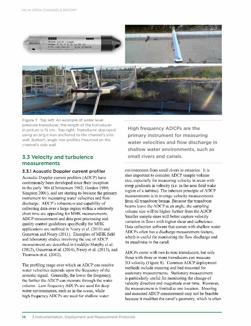
This indicates that the back water effect from the turbine deployment reached well upstream for this particular canal geometry. The extent of the flow disturbance upstream of the turbine is influenced by flow conditions and the canal geometries. As such, it can be difficult to optimize the location of water level sensors to get the most useful information with the minimum amount of expense (i.e. sensor and data processing costs, etc.); however numerical hydrodynamic models can prove useful for this purpose. A common instrument for monitoring water level is a water level pressure transducer. Pressure transducers make point measurements, are battery-powered and, depending on the data sampling rates, can be remotely deployed for measuring water levels for days or weeks (Figure 7). Water level could fluctuate significantly within seconds, therefore the highest sampling rate should be used whenever possible, to allow accurate assessment on water level dynamics. The transducer is commonly deployed at the side wall of a channel, such as the one shown in Figure 7. One way to deploy the transducer is by mounting it on a PVC pipe and sliding the pipe into an angle iron anchored to the channel wall. The water elevation at the measured location relative to a datum can be determined by taking into account the transducer’s depth measurement, the elevation of the top of the angle iron (which can be measured using a total station) and the vertical distance between the top of the angle iron and the transducer location.
While the near bank water level may differ from the centerline water level, the bank water level is the primary interest for water operators such as the USBR and local irrigation districts, because spillways, which release water into neighboring fields to prevent overtopping of the canal, are located at the bank of the canal. For that reason, measuring water levels at the channel’s sidewall is appropriate for overtopping assessment. Energy grade line should ideally be calculated using mean cross-section depths to take into account depth variations across the channel. This can be done using multiple pressure transducers mounted across the channel. However, installation of additional mounting hardware on the bottom is often required, and this is most easily done when no water is present in the canal.
Measuring continuous water levels across the channel requires an instrument that is capable of moving across the channel, such as an echo sounder mounted on a survey boat. Measurements using this method in the wake region are often challenging because of the highly turbulent flow and dynamic water surface elevation in that region.
Figure 6. Water level time series at the Roza Canal site, at 50 m and 700 m upstream of the turbine.
Hydrodynamic assessment should be performed for both baseline and turbine operation conditions. Water level measurements should be taken simultanouesly at several locations upstream and downstream of the turbine(s).
A water level pressure transducer can be used to continuously monitor water levels, and the highest sampling rate should be used if the levels fluctuate. To assess overtopping, water levels should be measured at the channel’s sidewall.
HK IN OPEN CHANNELS REPORT
Figure 7. Top left: An example of water level pressure transducer; the length of the transducer in picture is 15 cm. Top right: Transducer, deployed using an angle iron anchored to the channel’s side wall. Bottom: angle iron profiles mounted on the channel’s side wall.
3.3 Velocity and turbulence measurements3.3.1 Acoustic Doppler current profilerAcoustic Doppler current profilers (ADCP) have continuously been developed since their inception in the early ‘80s (Christensen 1982; Gordon 1989; Simpson 2001), and are starting to become the primary instrument for measuring water velocities and flow discharge. ADCP’s robustness and capability of collecting data over a large region within a relatively short time are appealing for MHK measurements. ADCP measurement and data post processing and quality control guidelines specifically for MHK applications are outlined in Neary et al. (2011) and Gunawan and Neary (2011). Examples of MHK field and laboratory studies involving the use of ADCP measurement are described in Goddijn-Murphy et al. (2012), Gunawan et al. (2014), Neary et al. (2013), and Thomson et al. (2012).
The profiling range over which an ADCP can resolve water velocities depends upon the frequency of the acoustic signal. Generally, the lower the frequency, the farther the ADCP can measure through the water column. Low frequency ADCPs are used for deep water environments, such as in the ocean, while high frequency ADCPs are used for shallow water
environments from small rivers to estuaries. It is also important to consider ADCP sample volume size, especially for measuring velocity in areas with steep gradients in velocity (i.e. in the near field wake region of a turbine). The inherent principle of ADCP measurements is to average velocity measurements from all transducer beams. Because the transducer beams leave the ADCP at an angle, the sampling volume size will be higher further from the ADCP. Smaller sample sizes will better capture velocity variation in flows with higher shear and turbulence. Data collection software that comes with shallow water ADCPs often has a discharge measurement feature, which is useful for monitoring the flow discharge and its steadiness in the canal.
ADCPs come with two to nine transducers, but only those with three or more transducers can measure 3D velocity (Figure 8). Common ADCP deployment methods include mooring and bed mounted for stationary measurements. Stationary measurement is particularly useful for monitoring the change of velocity direction and magnitude over time. However, the measurement is limited to one location. Mooring and mounted ADCP measurement may not be feasible because it modifies the canal’s geometry, which is often
14 3 Instrumentation, Deployment and Measurement Protocols
High frequency ADCPs are the primary instrument for measuring water velocities and flow discharge in shallow water environments, such as small rivers and canals.
3 Instrumentation, Deployment and Measurement Protocols 15
prohibited by the water district that manages the canal operation. Another common ADCP deployment method is the moving-vessel method, where the ADCP takes velocity profile measurements from a floating platform (often a boat) while it is moving. The ADCP can be moved by tethering the ADCP boat or by driving the boat if the boat is equipped with a motor.
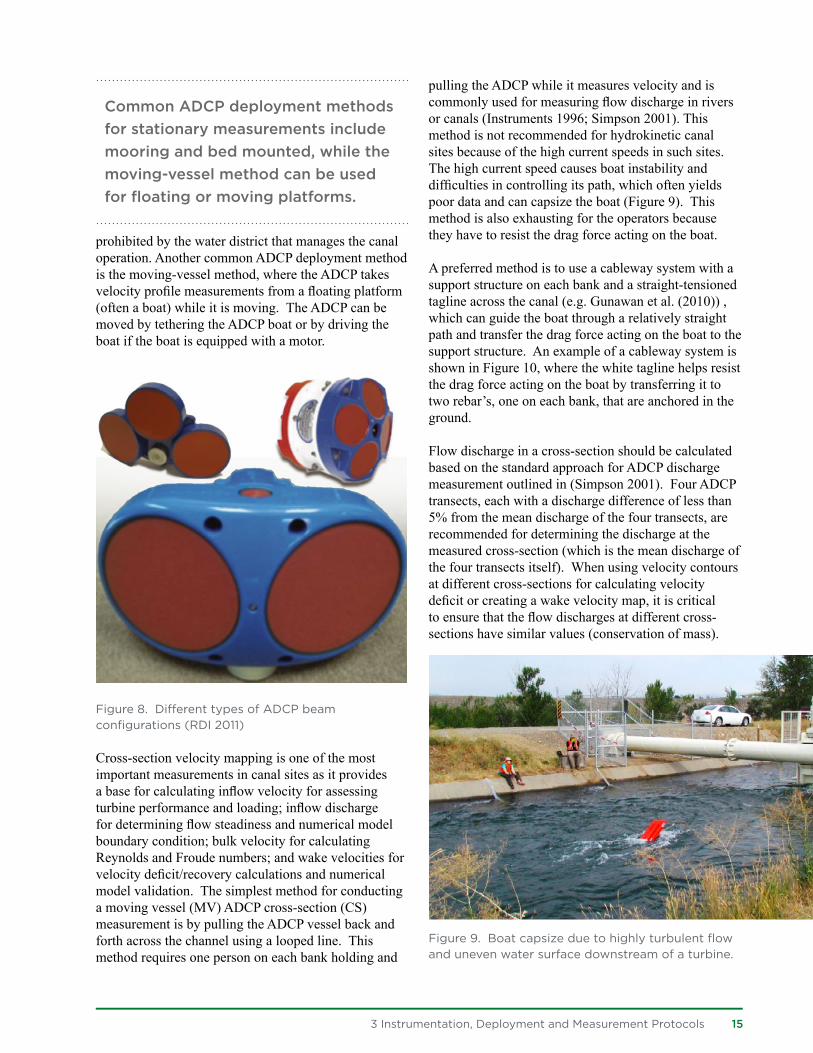
Figure 8. Different types of ADCP beam configurations (RDI 2011)
Cross-section velocity mapping is one of the most important measurements in canal sites as it provides a base for calculating inflow velocity for assessing turbine performance and loading; inflow discharge for determining flow steadiness and numerical model boundary condition; bulk velocity for calculating Reynolds and Froude numbers; and wake velocities for velocity deficit/recovery calculations and numerical model validation. The simplest method for conducting a moving vessel (MV) ADCP cross-section (CS) measurement is by pulling the ADCP vessel back and forth across the channel using a looped line. This method requires one person on each bank holding and
pulling the ADCP while it measures velocity and is commonly used for measuring flow discharge in rivers or canals (Instruments 1996; Simpson 2001). This method is not recommended for hydrokinetic canal sites because of the high current speeds in such sites. The high current speed causes boat instability and difficulties in controlling its path, which often yields poor data and can capsize the boat (Figure 9). This method is also exhausting for the operators because they have to resist the drag force acting on the boat.
A preferred method is to use a cableway system with a support structure on each bank and a straight-tensioned tagline across the canal (e.g. Gunawan et al. (2010)) , which can guide the boat through a relatively straight path and transfer the drag force acting on the boat to the support structure. An example of a cableway system is shown in Figure 10, where the white tagline helps resist the drag force acting on the boat by transferring it to two rebar’s, one on each bank, that are anchored in the ground.
Flow discharge in a cross-section should be calculated based on the standard approach for ADCP discharge measurement outlined in (Simpson 2001). Four ADCP transects, each with a discharge difference of less than 5% from the mean discharge of the four transects, are recommended for determining the discharge at the measured cross-section (which is the mean discharge of the four transects itself). When using velocity contours at different cross-sections for calculating velocity deficit or creating a wake velocity map, it is critical to ensure that the flow discharges at different cross-sections have similar values (conservation of mass).
Figure 9. Boat capsize due to highly turbulent flow and uneven water surface downstream of a turbine.
Common ADCP deployment methods for stationary measurements include mooring and bed mounted, while the moving-vessel method can be used for floating or moving platforms.

HK IN OPEN CHANNELS REPORT
16 3 Instrumentation, Deployment and Measurement Protocols
Figure 10. A cableway deployment with a tensioned tagline (the white line), that is attached to the ADCP boat.
When conducting cross-section measurements, the ADCP should be traversed slowly and at a constant speed to reduce noise in the data. Traversing too fast could introduce measurement errors, which could cause inaccurate discharge measurements. These errors can include invalid bottom tracking (Mueller and Wagner 2009) and bin resolution that is too coarse (Gunawan et al. 2011). At the Roza Canal site, which has a typical bulk velocity value of around 2 m/s and a typical water surface width of around 13 m, a traverse speed of 0.05 m/s was used to obtain consistent single-transect discharge values. The ADCP bin sizes during these measurements were set to 0.2 - 0.25 m. For these conditions, traverse speeds of greater than 0.10 m/s typically caused inconsistent single-transect discharge values. While there are currently no guidelines on optimal ADCP traverse speeds, a general rule of thumb is for the boat travel speed to be less than the water speed (Muller et al. 2013). The optimal
speed will likely be site specific, and is dependent on many parameters that can include, mean water speed, turbulence, suspended sediment concentration, and ADCP settings. Therefore, ADCP operators are advised to figure out the optimal traverse speed on their test site by taking measurements with different traverse speeds, and comparing the results.
Inflow velocity should be measured at an upstream cross-section where the velocity dip due to the presence of the turbine is not observed. The velocity dip diminishes typically at three or more turbine diameters upstream of the turbine. Velocity within the turbine wake begins to recover almost immediately but takes between 10 to 20 turbine diameters downstream of the turbine before the velocity reaches 80%-90% of its original inflow value (Chamorro et al. 2015; Maganga et al. 2010; Myers and Bahaj 2007; Myers and Bahaj 2010; Neary et al. 2013). For that reason, wake velocity measurements should include the region within 20 turbine diameters downstream from the turbine whenever possible. Figure 11 shows examples of an inflow cross-section velocity contour and three wake flow velocity contours measured at three different cross-sections at the Roza Canal site. The inflow velocity magnitudes are relatively uniform across the channel. The wake flow velocity contours show a deceleration in the middle of the channel due to the presence of the turbine, whereas accelerations are observed near the banks. The deceleration and accelerations are more pronounced immediately downstream of the turbine, but gradually diminish with increasing distance from the turbine.
The MV ADCP measurement method essentially collects short period (instantaneous) velocity data at each position of the ADCP. As a result, the velocity measurements contain large fluctuations due to flow turbulence and instrument noise and, hence, do not resemble the smooth-time-averaged velocity profiles generally used for open-channel flow analysis. This method, however, is favorable for most HK-related measurements due to its capability to achieve data from a large region within a short time. Data post-processing, such as spatio-temporal data averaging, is recommended prior to analyzing the data. Dinehart and Burau (2005), Szupiany et al. (2007), Gunawan et al. (2010), proposed spatio-temporal averaging methods to smooth the velocity contours measured using the MV method. Traversing the same transect several times and averaging the measurements at each reduces the fluctuations in velocity profiles, caused by flow turbulence and instrument errors.
A rebar support, anchored to the ground
Cross-section velocity mapping is important to calculate inflow velocity, inflow discharge, bulk velocity, and wake velocities. The preferred method of measurement is to use a cableway system and to traverse the ADCP slowly and at a constant speed.
3 Instrumentation, Deployment and Measurement Protocols 17
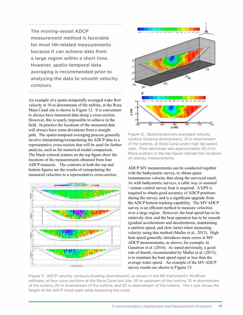
An example of a spatio-temporally averaged wake flow velocity at 10 m downstream of the turbine, at the Roza Main Canal site is shown in Figure 12. It is convenient to always have measured data along a cross-section. However, this is nearly impossible to achieve in the field. In practice the locations of the measured data will always have some deviations from a straight path. The spatio-temporal averaging process generally involve interpolating/extrapolating the ADCP data to a representative cross-section that will be used for further analysis, such as for numerical model comparison. The black-colored scatters on the top figure show the locations of the measurements obtained from four ADCP transects. The contours in both the top and bottom figures are the results of extrapolating the measured velocities to a representative cross-section.
Figure 12. Spatiotemporally-averaged velocity contour (looking downstream), 10 m downstream of the turbine, at Roza Canal under high tip-speed ratio. Flow discharge was approximately 55 m3/s. Black scatters in the top figure indicate the locations of velocity measurements.
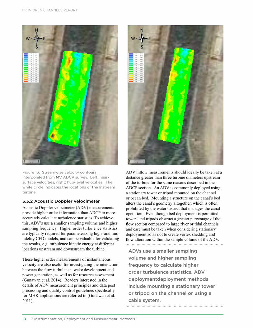
ADCP MV measurements can be conducted together with the bathymetric survey, to obtain quasi-instantaneous velocity data along the surveyed reach. As with bathymetric surveys, a cable way or manned / remote control survey boat is required. A GPS is required to obtain good accuracy of ADCP positions during the survey, and is a significant upgrade from the ADCP bottom tracking capability. The MV ADCP survey is an efficient method to measure velocities over a large region. However, the boat speed has to be relatively slow and the boat operation has to be smooth (gradual accelerations and decelerations, maintaining a uniform speed, and slow turns) when measuring velocity using this method (Muller et al., 2013). High boat speed generally introduces more errors in MV ADCP measurements, as shown, for example, in Gunawan et al. (2016). As stated previously, a good rule of thumb, recommended by Muller et al. (2013), is to maintain the boat speed equal or less than the average water speed. An example of the MV ADCP survey results are shown in Figure 13.
The moving-vessel ADCP measurement method is favorable for most HK-related measurements because it can achieve data from a large region within a short time. However, spatio-temperal data averaging is recommended prior to analyzing the data to smooth velocity contours.
Figure 11. ADCP velocity contours (looking downstream), as shown in the RD Instrument’s WinRiver software, at four cross-sections at the Roza Canal test site: 50 m upstream of the turbine, 10 m downstream of the turbine, 20 m downstream of the turbine, and 30 m downstream of the turbine. The x axis shows the length of the ADCP travel path while traversing the canal.
HK IN OPEN CHANNELS REPORT
Figure 13. Streamwise velocity contours, interpolated from MV ADCP survey. Left: near-surface velocities, right: hub-level velocities. The white circle indicates the locations of the Instream turbine.
3.3.2 Acoustic Doppler velocimeterAcoustic Doppler velocimeter (ADV) measurements provide higher order information than ADCP to more accurately calculate turbulence statistics. To achieve this, ADV’s use a smaller sampling volume and higher sampling frequency. Higher order turbulence statistics are typically required for parameterizing high- and mid-fidelity CFD models, and can be valuable for validating the results, e.g. turbulence kinetic energy at different locations upstream and downstream the turbine.
These higher order measurements of instantaneous velocity are also useful for investigating the interaction between the flow turbulence, wake development and power generation, as well as for resource assessment (Gunawan et al. 2014). Readers interested in the details of ADV measurement principles and data post processing and quality control guidelines specifically for MHK applications are referred to (Gunawan et al. 2011).
ADV inflow measurements should ideally be taken at a distance greater than three turbine diameters upstream of the turbine for the same reasons described in the ADCP section. An ADV is commonly deployed using a stationary tower or tripod mounted on the channel or ocean bed. Mounting a structure on the canal’s bed alters the canal’s geometry altogether, which is often prohibited by the water district that manages the canal operation. Even though bed deployment is permitted, towers and tripods obstruct a greater percentage of the flow section compared to large river or tidal channels and care must be taken when considering stationary deployment so as not to create vortex shedding and flow alteration within the sample volume of the ADV.
ADVs use a smaller sampling volume and higher sampling frequency to calculate higher order turbulence statistics. ADV deploymentdeployment methods include mounting a stationary tower or tripod on the channel or using a cable system.
18 3 Instrumentation, Deployment and Measurement Protocols

3 Instrumentation, Deployment and Measurement Protocols 19
The ADV sampling volume, whenever feasible, should be placed at the turbine hub height or rotor mid height level. This ADV position is anticipated to provide the most representative inflow to the turbine and the maximum deficit in the wake of the turbine. Further, it is beneficial to cover the ADV stem (mounting pole) with a hydrofoil to minimize drag on the ADV support structure. This helps in reducing the vibration of the measurement probe and lessen flow diversions to the location of the sampling volume; both introduce error in the velocity measurement.
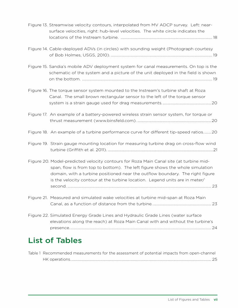
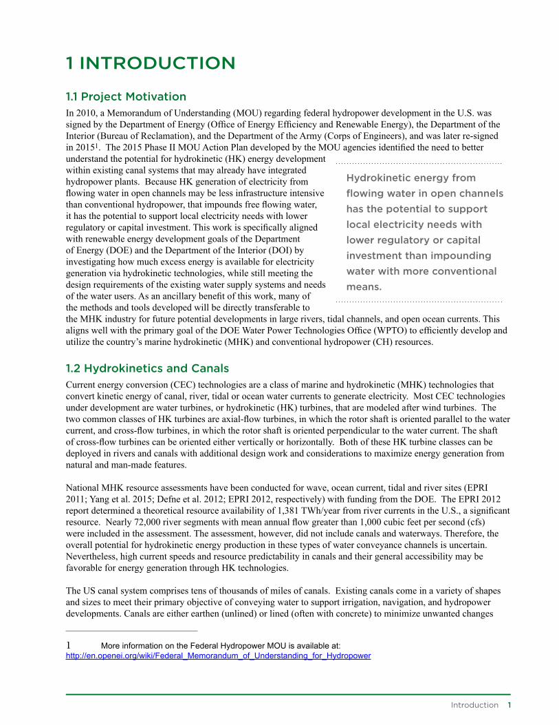
Another ADV deployment method suitable for canal measurements is cable deployment. An example of a cable-deployed ADV using a sounding weight, deployed from a boat, is outlined in Holmes and Garcia (2008) (Figure 14). If the width of the canal is relatively small, a cableway system, mounted at the canal edges, may be used to deploy the ADV (Figure 15). The cabled ADV was mounted to two tensioned-steel wires using an aluminum plate. The system is designed to be able to move the ADV laterally and vertically, and significantly withstand the water flow-induced drag force to up to 1-meter depth below the water surface. It should be noted that the ADV will likely move (swing) during cable deployment due to the flow drag and turbulence. If the errors caused by the ADV motions are significant, the measurement may need to be discarded. Accounting for flow induced motion of the ADV on the velocity measurements is an ongoing research topic. Several researchers have suggested correction methods and performed limited testing using the methods (Thomson et al., 2015, Durgesh et al., 2014, Neary et al., 2012). Readers interested in learning more about these correction methods are advised to review these references.
Figure 15. Sandia’s mobile ADV deployment system for canal measurements. On top is the schematic of the system and a picture of the unit deployed in the field is shown on the bottom.
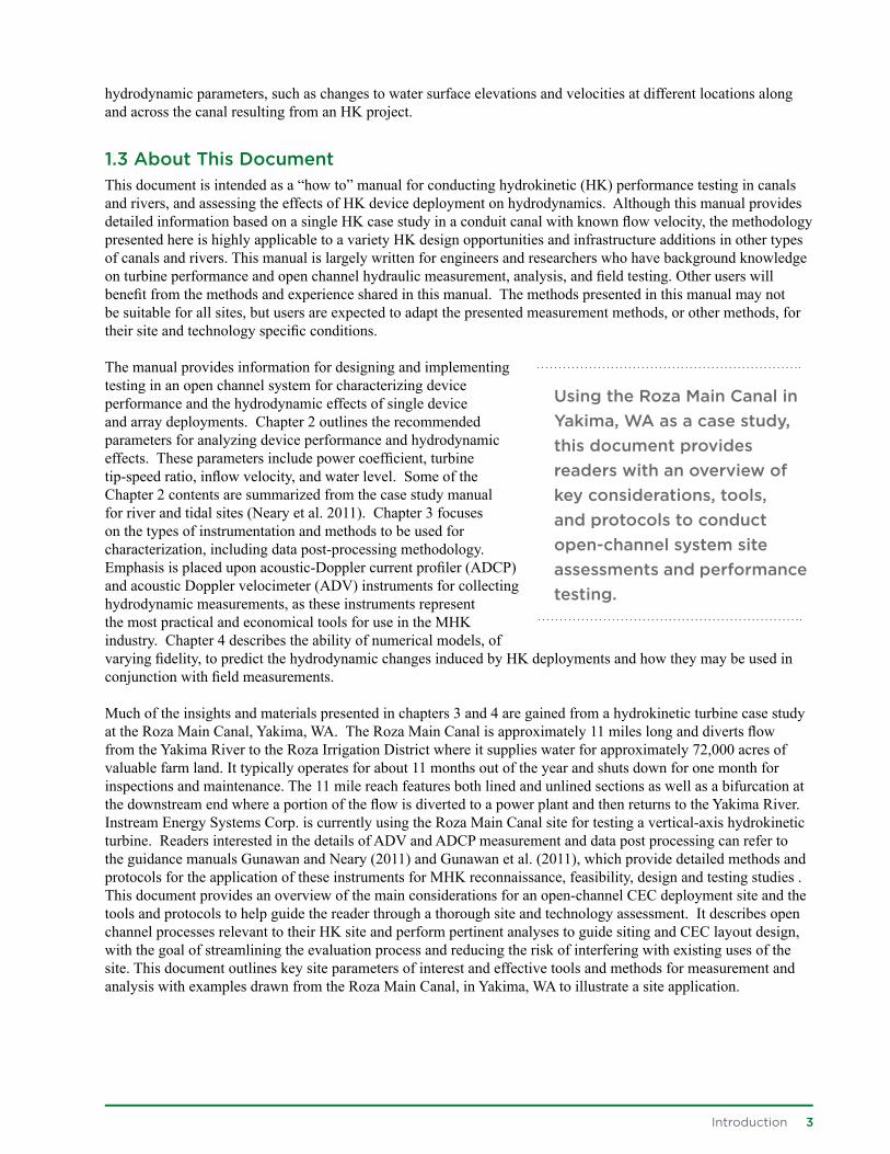
3.4 Power measurementTurbine power time series for assessing power production performance can be obtained from generator output or by measuring the rotor’s mechanical torque and angular velocity. Common methods for torque measurements include mounting a strain gauge at the shaft. The technical challenges for this method are supplying power to the strain gauge through the rotating shaft and sending the signal out of the rotating shaft. Slip rings can be used to interface to the rotating shaft, but they are susceptible to wear and need to be replaced over time. A non-contact method for transferring the power into and signal out of the shaft eliminates the needs of a slip ring. This method typically uses radio telemetry and wireless induced power and an example can be seen in Figure 16. The system in this example consists of a stationary power coil and a rotating collar that needs to be mounted on the shaft. A torque strain gauge is mounted to the shaft and connected to the rotating collar. Wireless power and data transmission occur in the small gap between the stationary coil and rotating collar. The size of the gap is maintained constant while the collar is rotating with the shaft. The collar is equipped with six magnets that can be tracked by the magnet sensor located in the master control unit to enable angular velocity measurement of the shaft.
If only temporary torque measurement is required, a battery-powered wireless system can be used (Figure 17). The torque measurement principle of the battery-powered (BP) system is similar to the wireless collar system. However, a power coil is not needed for the BP system, which reduces the complexity of the system installation significantly. The BP system consists of a radio transmitter that can be mounted to the shaft using a strong tape, such as a fiberglass one, and a receiver
Figure 14. Cable-deployed ADVs (in circles) with sounding weight (Photograph courtesy of Bob Holmes, USGS, 2010).
HK IN OPEN CHANNELS REPORT
20 3 Instrumentation, Deployment and Measurement Protocols
for receiving the measurement signal. A torque strain gauge is mounted to the shaft and connected to the radio transmitter. A single 9V battery will typically last for a few hours of measurements. Multiple batteries allow longer measurements to be performed, but may not be practical because all of the batteries need to be mounted to the shaft.
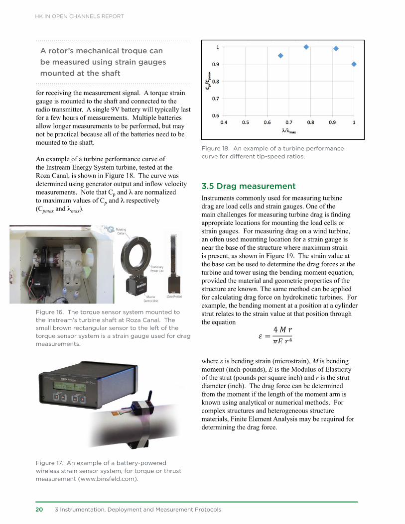
An example of a turbine performance curve of the Instream Energy System turbine, tested at the Roza Canal, is shown in Figure 18. The curve was determined using generator output and inflow velocity measurements. Note that Cp and l are normalized to maximum values of Cp and l respectively (Cpmax and lmax).
Figure 16. The torque sensor system mounted to the Instream’s turbine shaft at Roza Canal. The small brown rectangular sensor to the left of the torque sensor system is a strain gauge used for drag measurements.
Figure 17. An example of a battery-powered wireless strain sensor system, for torque or thrust measurement (www.binsfeld.com).
Figure 18. An example of a turbine performance curve for different tip-speed ratios.
3.5 Drag measurementInstruments commonly used for measuring turbine drag are load cells and strain gauges. One of the main challenges for measuring turbine drag is finding appropriate locations for mounting the load cells or strain gauges. For measuring drag on a wind turbine, an often used mounting location for a strain gauge is near the base of the structure where maximum strain is present, as shown in Figure 19. The strain value at the base can be used to determine the drag forces at the turbine and tower using the bending moment equation, provided the material and geometric properties of the structure are known. The same method can be applied for calculating drag force on hydrokinetic turbines. For example, the bending moment at a position at a cylinder strut relates to the strain value at that position through the equation
where ε is bending strain (microstrain), M is bending moment (inch-pounds), E is the Modulus of Elasticity of the strut (pounds per square inch) and r is the strut diameter (inch). The drag force can be determined from the moment if the length of the moment arm is known using analytical or numerical methods. For complex structures and heterogeneous structure materials, Finite Element Analysis may be required for determining the drag force.
A rotor’s mechanical troque can be measured using strain gauges mounted at the shaft
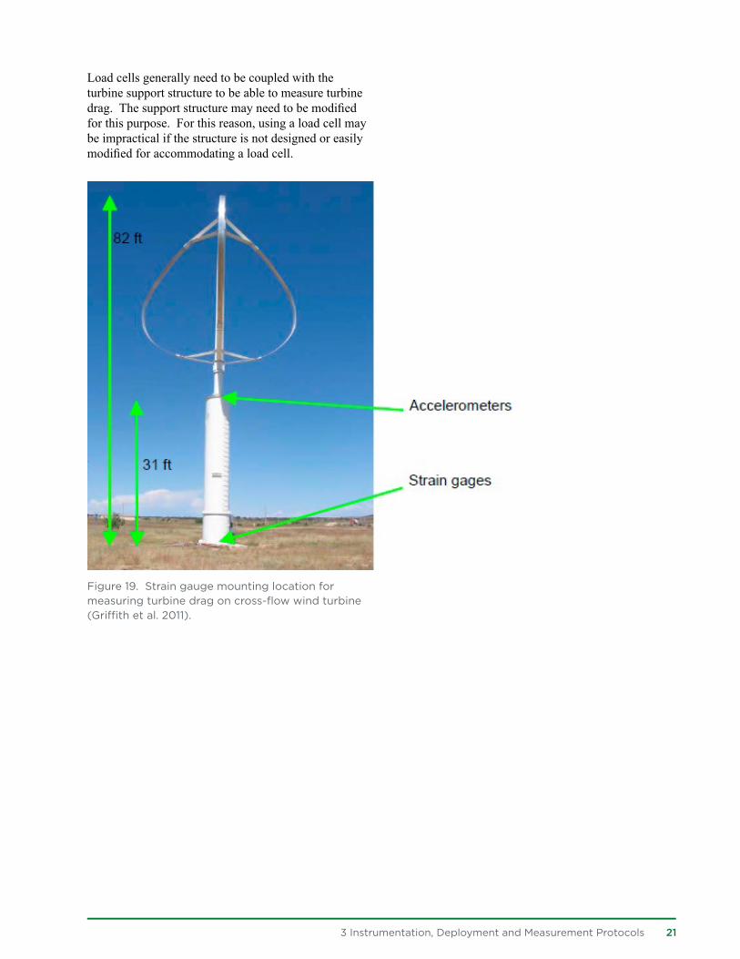
3 Instrumentation, Deployment and Measurement Protocols 21
Load cells generally need to be coupled with the turbine support structure to be able to measure turbine drag. The support structure may need to be modified for this purpose. For this reason, using a load cell may be impractical if the structure is not designed or easily modified for accommodating a load cell.
Figure 19. Strain gauge mounting location for measuring turbine drag on cross-flow wind turbine (Griffith et al. 2011).
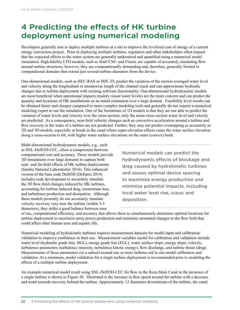
HK IN OPEN CHANNELS REPORT
4 Predicting the effects of HK turbine deployment using numerical modelingDevelopers generally aim to deploy multiple turbines at a site to improve the levelized cost of energy of a current energy conversion project. Prior to deploying multiple turbines, regulators and other stakeholders often request that the expected effects to the water system are generally understood and quantified using a numerical model simulation. High-fidelity CFD models, such as StarCCM+ and Fluent, are capable of accurately simulating flow around turbine structures, however, they are computationally demanding and, therefore, generally limited to computational domains that extend just several turbine diameters from the device.
One-dimensional models, such as HEC-RAS or ISIS 1D, predict the variation of the section averaged water level and velocity along the longitudinal or streamwise length of the channel reach and can approximate hydraulic changes due to turbine deployment with existing software functionality. One-dimensional hydrodynamic models are most beneficial when operational impacts (mainly raised water levels) are the main concern and can predict the quantity and locations of HK installations as an initial estimation over a large domain. Feasibility level results can be obtained faster and cheaper compared to more complex modeling tools and generally do not require a numerical modeling expert to run the simulation. One of the limitations of 1D models is that they are not able to predict the variation of water levels and velocity over the cross-section; only the mean cross-section water level and velocity are predicted. As a consequence, near-field velocity changes such as convective acceleration around a turbine and flow recovery in the wake of a turbine are not predicted. Further, they may not predict overtopping as accurately as 2D and 3D models; especially at bends in the canal where super-elevation effects cause the water surface elevation along a cross-section to tilt, with higher water surface elevations on the outer (convex) bank.
Multi-dimensional hydrodynamic models, e.g., such as SNL-Delft3D-CEC, allow a compromise between computational cost and accuracy. These models provide 3D simulations over large domains to capture both near- and far-field effects of HK turbine deployments (Sandia National Laboratories 2016). This enhanced version of the base code Delft3D (Deltares 2014) includes code development to accurately simulate the 3D flow-field changes induced by HK turbines, accounting for turbine induced drag, momentum loss, and turbulence production and dissipation. Although these models presently do not accurately simulate velocity recovery very near the turbine (within 3-5 diameters), they strike a good balance between ease of use, computational efficiency, and accuracy that allows them to simultaneously determine optimal locations for turbine deployment to maximize array power production and minimize unwanted changes to the flow field that could affect other human uses and aquatic life.
Numerical modeling of hydrokinetic turbines requires measurement datasets for model input and calibration/validation to improve confidence in their use. Measurement variables useful for calibration and validation include water level (hydraulic grade line, HGL), energy grade line (EGL), water surface slope, energy slope, velocity, turbulence parameters (turbulence intensity, turbulence kinetic energy), flow discharge, and turbine thrust (drag). Measurements of these parameters (or a subset) around one or more turbines aid in site model calibration and validation. At a minimum, model validation for a single turbine deployment is recommended prior to modeling the effects of a multiple turbine deployment.
An example numerical model result using SNL-Delft3D-CEC for flow in the Roza Main Canal in the presence of a single turbine is shown in Figure 20. Illustrated is the increase in flow speed around the turbine with a decrease and trend towards recovery behind the turbine. Approximately 12 diameters downstream of the turbine, the canal
22 4 Predicting the effects of HK turbine deployment using numerical modeling
Numerical models can predict the hydrodynamic effects of blockage and drag caused by hydrokinetic turbines and assess optimal device spacing to maximize energy production and minimize potential impacts, including local water level rise, scour, and deposition.

4 Predicting the effects of HK turbine deployment using numerical modeling 23
boundary surface transitions from concrete lining to earthen lining (unlined), and nearly doubles in width. Geometry transitions increase the challenges for in-situ field data collection and numerical modeling. It also complicates the assessment of flow recovery in the lee of the turbine. A common calibration/validation approach for MHK turbine simulations is to compare measured and simulated centerline hub/mid rotor height wake velocities, as shown in the example in Figure 21. Note that the measurement data shown was obtained from MV ADCP measurements (interpolated), which include several along cross-section MV measurements, and a survey measurement in which the ADCP/survey boat was moved in a zig-zag pattern over the measurement area. This is best done in a straight section of channel to minimize aforementioned super-elevation effects. Results from the model compare well with measurements from the collected field data of velocity recovery behind the deployed turbine starting 4 diameters in the wake of the turbine. To maximize power production, it is best to deploy turbines far enough apart such that velocity recovery and rate of recovery from the upstream turbine to the downstream turbine has reached a balance. This often occurs within 7-20 diameters downstream of the upstream turbine (Myers and Bahaj 2010, Stallard et. Al 2013, Chamorro et. Al 2015). Although SNL-Delft3D-CEC doesn’t capture the very near field-field velocity deficit (3-5 diameters) it is still well suited for determining the optimal spacing requirements.
Figure 20. Model-predicted velocity contours for Roza Main Canal site (at turbine mid-span, flow is from top to bottom). The left figure shows the whole simulation domain, with a turbine positioned near the outflow boundary. The right figure is the velocity contour at the turbine location. Legend units are in meter/second.
Numerical simulations also need to be able to predict the Hydraulic and Energy Grade Lines (HGL and EGL) accurately, with and without the turbine’s presence, because they are main parameters for quantifying HK deployment effects. Water level and velocity measurements can be used for assessing the model’s performance in this aspect. The predicted changes of water level and bulk (cross-section averaged) velocity along the reach without the turbine and with the turbine in place can be assessed against measurements. The same measurements can also be used for validating the water surface and energy slope predicted by the model. For example, the model predicted HGLs and EGLs at the Roza Main Canal for baseline (without turbine’s presence) and in the turbine’s presence are shown in Figure 22. The model predicts that adding a turbine at the present location increases water levels by around 6 centimeters immediately upstream of the turbine and around 3 centimeters at 700 m (~233 diameters) upstream of the turbine; these values are close to the 4 and 3 centimeters obtained from
Water level, energy grade line water surface slope, energy slope, velocity, turbulence parameters, flow discharge, and turbine drag are all measurement variables useful for calibrating and validating numeric models.

HK IN OPEN CHANNELS REPORT
24 4 Predicting the effects of HK turbine deployment using numerical modeling
measurements respectively. In addition, the predicted water surface slope along the reach also agrees well with the measured value. Once the single turbine model is calibrated and validated against measurements (e.g. thrust (drag) coefficient), the turbine calibration parameters can be used for multiple-turbine simulation cases, for project optimization.
Figure 21. Measured and simulated wake velocities at turbine mid-span at Roza Main Canal, as a function of distance from the turbine.
Figure 22. Simulated Energy Grade Lines and Hydraulic Grade Lines (water surface elevations along the reach) at Roza Main Canal with and without the turbine’s presence.

5 Summary 25
5 SummaryAlthough a detailed hydrokinetic canal resource assessment does not exist at this time, it is clear that some existing canal systems contain favorable flow speeds, water depths, and other characteristics that are desirable for hydrokinetic power development. Feasibility studies for HK projects must demonstrate that HK operations will not adversely affect water operations. Potential concerns include disrupting water supply operations (by affecting head-discharge conditions at irrigation canal intakes), flooding (when turbine deployment and operation increase water levels above acceptable limits), reduction of power generation in nearby hydropower plant (by affecting the water levels and net head at hydropower dam or discharge), and unfavorable erosion-deposition patterns. Carefully thought out physical and numerical tests can be used to address these issues and determine the viability of a particular canal or section of a canal for various amounts of HK energy development. This document should be viewed as a starting point to identify the parameters to be measured, instrumentation and deployment strategies for their measurements, and protocols for acquiring and processing data, for HK flow effects and turbine performance assessments within canals (and potentially small rivers).
To help estimate the level of effort required for a hydrokinetic assessment and impact study, Table 1 summarizes required data and potential methods for collecting that data. Table 1 assumes a full hydrodynamic impact study with an operational HK turbine installed. This effort could take a few weeks to several months depending on scheduled discharges, site conditions, and HK turbine design. For example, an HK installation that can hoist its own turbine in and out of the flow can be compared to the exact same baseline conditions on the same day and testing could be completed within a matter of days for a given flow condition. In contrast, a HK design that requires a flow shutdown to install or remove the unit may require months to acquire sufficient baseline data and several months after the installation for comparison to HK operational data under similar flow conditions. For a feasibility level study, bathymetry, discharge, and water level data at key locations of the channel (transitions, bifurcations, siphons, flow measurement structures, etc.) are sufficient to help determine if HK deployment is an option. This information is often available from owners and operators of the canal and can be verified using methods identified in Table 1. As previously mentioned, these data can be used with numerical models to support feasibility studies.
Table 1 Recommended measurements for the assessment of potential impacts from open-channel HK operations
Note that the measurements listed in table 1 are also required for numerical model input, and HGL and EGL calculations.
Table 1 Recommended measurements for the assessment of potential impacts from open-channel HK operations
No Measurement Parameters Locations Main Purpose Instrument
Example
1 Bathymetry (or geometry for lined channels)
Along the channel, within 20 - 30 diameter from the turbine, and far upstream of the turbine, at the same locations with far upstream water level measurements
Determine channel bed elevations, or verify the existing bathymetry data (as-built geometry data can suffice for lined channels if verified by a field survey)
echo sounder and remotely-controlled survey boat
2 Water level Cross sections immediately upstream and downstream of the turbine, e.g. every diameter within 5 diameters from the turbine, and every 3-5 diameters between 5 to 20 diameters from the turbine.
Determine impact on water level at locations adjacent to the turbine, where significant difference from baseline (without HK) is often expected
water level logger

HK IN OPEN CHANNELS REPORT
26 5 Summary
No Measurement Parameters Locations Main Purpose Instrument
Example
3 Water level Cross sections far upstream of the turbine, e.g. at -100, -200 and -300 x/D
Determine impact on water level at far upstream of the turbine. Impact at far upstream is typically expected for open channels with subcritical flow.
water level logger
4 Downstream local velocity measurement over entire cross-section
Cross sections every 1 or 2 diameters up to 5 diameters downstream; every 2 to 5 diameters between 5 and 20 diameters downstream
Determine local velocity variations downstream of the turbine, where high velocity gradients are expected. This information is useful for turbine array design and erosion/deposition/scouring/silting analysis.
ADCP
5 Upstream local velocity measurement over entire cross-section
Cross sections at 5 and 10 diameters upstream
Determine inflow velocity for establishing turbine performance curves, as well as velocity gradients.
ADCP
6 Upstream and downstream velocity and turbulence, at a high sampling resolution
Ideally at the same cross sections as the upstream and downstream ADCP measurements, at turbine centerline. A minimum of 3 locations downstream and one location upstream (between 5 to 10 diameter upstream) is required for numerical model input.
Determine turbulence level and unsteady coherent structures on the flow. This information is useful for identifying and quantifying cyclical load on the turbine, and is a critical numerical model input for accurately predicting wake profiles.
ADV
Note that the measurements listed in table 1 are also required for numerical model input, and HGL and EGL calculations.
6 References 27
6 ReferencesChamorro, L. P., Hill, C., Neary, V. S., Gunawan, B., Arndt, R. E. A., and Sotiropoulos, F. (2015). “Effects of energetic coherent motions on the power and wake of an axial-flow turbine.” Physics of Fluids, 27(5), 055104.
Christensen, J. L. H., L.E. (1982). “Mississippi River test “ Vol. 1, U.S. Geological Survey, El Cajon, CA.
Defne, Z., Haas, K. A., Fritz, H. M., Jiang, L. D., French, S. P., Shi, X., Smith, B. T., Neary, V. S., and Stewart, K. M. (2012). “National geodatabase of tidal stream power resource in USA.” Renewable and Sustainable Energy Reviews, 16(5), 3326-3338.
Deltares (2014). “Delft3D: Hydro-Morphodynamics.” Deltares: Delft, Netherlands. p. 712.
Dinehart, R. L., and Burau, J. R. (2005). “Averaged indicators of secondary flow in repeated acoustic Doppler current profiler crossings of bends.” Water Resour Res, 41(9).
Durgesh,V., Thomson, J., Richmond, M.C., Polagye,B. (2014) “Noise correction of turbulent spectra obtained from acoustic doppler velocimeters.” Flow Measurement and Instrumentation, Volume 37, June, Pages 29-41.
EPRI (2011). “Mapping and Assessment of the United States Ocean Wave Energy Resource. .” R. b. E. P. R. I. E. a. N. R. E. L. (NREL). ed., pp 176.
EPRI (2012). Assessment and mapping of the riverine hydrokinetic resource in the continental United States. No. 1026880. Electric Power Research Institute (EPRI).
Eye4Software (2015). “Hydromagic: Professional hydrographic survey software.” Software manual.
Goddijn-Murphy, L., Woolf, D. K., and Easton, M. C. (2012). “Current Patterns in the Inner Sound (Pentland Firth) from Underway ADCP Data.” Journal of Atmospheric and Oceanic Technology, 30(1), 96-111.
Gordon, R. L. (1989). “Acoustic Measurement of River Discharge.” Journal of Hydraulic Engineering-ASCE 115(7):925-936.
Griffith, D. T., Mayes, R., and Hunter, P. (2011). “Excitation Methods for a 60 kW Vertical Axis Wind Turbine.” Structural Dynamics and Renewable Energy, Volume 1, T. Proulx, ed., Springer New York, 329-338.
Gunawan, B., Neary, V., Roberts, J., Dallman, A., Grovue, S., Mortensen, J., and Heiner, B. (2014). “Field measurement test plan to determine effects of hydrokinetic turbine deployment on canal test site in Yakima, WA, USA.” Proceedings of the 2nd Marine Energy Technology Symposium (METS2014) Seattle, WA.
Gunawan, B., and Neary, V. S. (2011). “ORNL ADCP Post processing guide and Matlab algorithms for MHK site flow and turbulence analysis.” ORNL/TML-2011/404.
Gunawan, B., Neary, V. S., and Colby, J. (2014). “Tidal energy site resource assessment in the East River tidal strait, near Roosevelt Island, New York, New York.” Renewable Energy, 71, 509-517.
Gunawan, B., Neary, V. S., Hill, C., and Chamorro, L. (2011). “Accuracy of spatial and temporal averaging of acoustic Doppler current profiler (ADCP) moving boat measurements.” American Geophysical Union Fall Meeting, San Francisco, CA.
Gunawan, B., Neary, V.S. and Hill, C. (2016) “Comparison of fixed and moving vessel ADCP measurements in a large laboratory flume”. Journal of Hydraulic Engineering (in press).

HK IN OPEN CHANNELS REPORT
28 6 References
Gunawan, B., Neary, V. S., and McNutt, J. R. (2011). “ORNL ADV Post processing guide and Matlab algorithms for MHK site flow and turbulence analysis.” ORNL/TML-2011/338.
Gunawan, B., Sterling, M., and Knight, D. W. (2010). “Using an acoustic Doppler current profiler in a small river.” Water Environ J, 24(2), 147-158.
Hill, C., Neary, V. S., Gunawan, B., Guala, M., and Sotiropoulos, F. (2014). “U.S. Department of Energy Reference Model Program, RM1: Experimental Results.” Sandia Report, ed. No. SAND2014-18783R. Sandia National Laboratories (SNL-NM), Albuquerque, NM (United States).
Hill, C., Neary, V. S., Gunawan, B., Guala, M., and Sotiropoulos, F. (2014). “U.S. Department of Energy Reference Model Program, RM2: Experimental Results.” Sandia Report, ed. No. SAND2014-16561 R. Sandia National Laboratories (SNL-NM), Albuquerque, NM (United States).
Holmes, R. R., and Garcia, M. H. (2008). “Flow over bedforms in a large sand-bed river: A field investigation.” Journal of Hydraulic Research, 46(3), 322-333.
Instruments, R. (1996). “Acoustic Doppler Current Profiler: Principles of operation, a practical primer.” Technical manual.
Maganga, F., Germain, G., King, J., Pinon, G., and Rivoalen, E. (2010). “Experimental characterisation of flow effects on marine current turbine behaviour and on its wake properties.” IET Renewable Power Generation, 4(6), 498-509.
Mueller, D. S., and Wagner, C. R. (2009). “Measuring Discharge with Acoustic Doppler Current Profilers from a Moving-Boat.”
Mueller, D.S., Wagner, C.R., Rehmel, M.S., Oberg, K.A,, and Rainville, Francois, (2013), “Measuring discharge with acoustic Doppler current profilers from a moving boat” (ver. 2.0, December 2013): U.S. Geological Survey Techniques and Methods, book 3, chap. A22, 95 p. http://dx.doi.org/10.3133/tm3A22.
Myers, L., and Bahaj, A. S. (2007). “Wake studies of a 1/30th scale horizontal axis marine current turbine.” Ocean Engineering, 34(5-6), 758-762.
Myers, L. E., and Bahaj, A. S. (2010). “Experimental analysis of the flow field around horizontal axis tidal turbines by use of scale mesh disk rotor simulators.” Ocean Engineering, 37(2-3), 218-227.
Neary, V. S., Gunawan, B., Hill, C., and Chamorro, L. P. (2013). “Near and far field flow disturbances induced by model hydrokinetic turbine: ADV and ADP comparison.” Renewable Energy, 60(0), 1-6.
Neary, V. S., Gunawan, B., Polagye, B., Thomson, J., Richmond, M. C., Durgesh, V., Muste, M., and Fontaine, A. (2011). “Field measurements at river and tidal current sites for hydrokinetic energy development: Best practices manual.” ORNL/TML-2011/419.
Neary, V.S., Gunawan, B., Mellin, A. and Smith, B.T (2012) Sensor-fusion technology for accurate measurements in deep water environments. Invention Disclosure 201202876, S-124,449.
OceanScience, T. (2015). “Z-Boat 1800 Remote hydrographic survey boat.” Brochure.
Sandia National Laboratories (2016) “SNL-Delft3D-CEC.” Web article (http://energy.sandia.gov/energy/renewable-energy/water-power/market-acceleration-deployment/snl-delft3d-cec/). Last accessed: 12/19/2016.

6 References 29
Simpson, M. R. (2001). “Discharge Measurements Using a Broad-Band Acoustic Doppler Current Profiler “ open-file report 01-1., S. United States Geological Survey, ed.
Stallard, T., Collings, R., Feng, T., Whelan, J. (2013) “ Interactions between tidal turbine wakes: experimental study of a group of three-bladed rotors.” Phil. Trans. R. Soc. A 2013 371 20120159; DOI: 10.1098/rsta.2012.0159. Published 14 January 2013
Sturm, T. W. (2001). Open channel hydraulics.
Szupiany, R. N., Amsler, M. L., Best, J. L., and Parsons, D. R. (2007). “Comparison of fixed- and moving-vessel flow measurements with an aDp in a large river.” ASCE Journal of Hydraulic Engineering, 133(12), 1299-1309.
Te Chow, V. (1959). Open-channel hydraulics, McGraw-Hill.
Thomson, J., Polagye, B., Durgesh, V., and Richmond, M. C. (2012). “Measurements of Turbulence at Two Tidal Energy Sites in Puget Sound, WA.” IEEE Journal of Oceanic Engineering, 37(3), 363-374.
Thomson, J., Talbert, J., Klerk, A. D., Zippel, S., Guerra., M. and Kilcher, L. (2015) Turbulence measurements from moving platforms, 2015 IEEE/OES Eleveth Current, Waves and Turbulence Measurement (CWTM), St. Petersburg, FL, 2015, pp. 1-5.
US Army Corps of Engineer (1994) “Channel stability assessment for flood control projects.” EM 1110-2-1418, 31 October 1994 (retreived from http://www.publications.usace.army.mil/Portals/76/Publications/EngineerManuals/EM_1110-2-1418.pdf in December 8, 2016).
Yang, X., Haas, K. A., Fritz, H. M., French, S. P., Shi, X., Neary, V. S., and Gunawan, B. (2015). “National geodatabase of ocean current power resource in USA.” Renewable and Sustainable Energy Reviews, 44(0), 496-507.

For more information, visit: energy.gov/eere
DOE/EE-1537 • March 2017