ASME Paper GT2012-69587 Final 20120210 - DLR Portalelib.dlr.de/85778/1/Paper_GT2012-69587_Final.pdf2...

1 Copyright © 2012 by ASME

Proceedings of ASME Turbo Expo 2012 GT2012

June 11-15, 2012, Copenhagen, Denmark

GT2012-69587

DESIGN OF AN ECONOMICAL COUNTER ROTATING FAN – COMPARISON OF THE CALCULATED AND MEASURED STEADY AND UNSTEADY RESULTS

Timea Lengyel-Kampmann German Aerospace Center

Institute of Propulsion Technology Cologne, Germany

Email: [email protected]

Andreas Bischoff German Aerospace Center


Dr. Robert Meyer German Aerospace Center

Institute of Propulsion Technology Berlin, Germany

Dr. Eberhard Nicke German Aerospace Center


ABSTRACT Within the framework of the EU funded Project VITAL,

SNECMA (Group Safran), as the work package leader, developed a counter rotating low-speed fan-concept for a high bypass ratio engine. The detailed aerodynamic and mechanical optimization of one blading version (CRTF2.b) was carried out at the German Aerospace Center (DLR), by applying one of the newest design methods featuring a multi-objective automatic optimization method based on an Evolutionary Algorithm [1].

The final design goals were high efficiency, a sufficient stall margin and adequate acoustic performances for the given cycle parameters. The fan stage developed was tested in an anechoic test facility at CIAM in Moscow. The test routine included the measurement of the performance map based on total pressure and total temperature measurements at the inlet and the outlet of the test rig and acoustic measurement as well.

The unsteady flow field of the low speed Contra-Rotating Turbo Fan has been measured with four hot-wire probes at different axial positions.

In the evaluation the measured data are compared with high resolution CFD results. Special emphasis was given to the comparison of the radial distribution of total pressure and total temperature in the bypass channel, the comparison of the measured and the calculated fan maps and to the comparison of the hot-wire measurements with high resolution, unsteady CFD results. The tests and the URANS-results confirmed the design goals.

INTRODUCTION To reduce the fuel consumption, the NOx, CO2 emissions and the noise simultaneously proved to be a big challenge for the aircraft industry. The report "European Aeronautics: A Vision for 2020" written by the ACARE-Group [2] was the guideline for many national and international research programs like VITAL. A new revolutionary engine technology is necessary to meet the ACARE goals. One promising technology is the ducted counter-rotating fan with very high bypass ratio (BPR).

The project leading company, SNECMA, defined three different versions of counter-rotating fans with different design goals:

• CRTF1 was the baseline design by SNECMA for titanium blades

• CRTF2a has targeted at high level performance and low noise with composite blades, designed by CIAM

• CRTF2b has targeted at high level integration at low cost, which should be realized with a reduced number of blades, reduced axial length and with composite blades. This version was aerodynamically and mechanical designed by DLR.

The mentioned constraints of the CRTF2b, fewer blades,

reduced axial gap between the rotors and composite material for the blades targeted the saving of the engine weight.


The design criteria for composite blades were defined by a detailed blade thickness distribution by SNECMA, which led to significant increased blade thickness compared with CRTF1. Both, 20% reduced blade number and increased blade thickness lead to increased blade loading which are disadvantages to achieve high fan-efficiency. The acoustic impact of changes in blade counts and axial gap was not considered in detail during the design phase. The design and optimization process of the DLR considered and met all the previously mentioned constraints and targets. In spite of them the CFD calculations of the CRTF2b resulted in a high efficiency level. Simultaneously the required stall margin was achieved.

The experimental analysis and the comparison of the experimental and calculated results of the CRTF2b are the main focus of this work. The design and optimization method was described in detail in [2].

A short overview about the design and manufacturing process will be given at the beginning of the paper. The test, the instrumentation and the assembly of the CRTF2b at CIAM will be presented [15]. Hot-wire probes were installed in the test rig to measure the unsteady flow field. The probes were placed upstream of the first rotor, between the two rotors and downstream of the second rotor [6]. With the DLR hot-wire measuring technique, unsteady flow structures (e.g. the wake of each individual rotor blade) were measured and analyzed in detail. The average mean vectors as well as the fluctuating components of the velocity were determined. Parallel to the test additional CFD calculations with high geometrical- and mesh-resolution were carried out for the better comparability of the experimental and CFD results. This will be discussed in this paper as well.

The experimental results were required to validate the CFD results and the reliability of the in-house optimizer AutoOpti [1].

NOMENCLATURE ADP aerodynamic design point AP Aircraft Philipp BL Boundary layer BPR Bypass ratio CR counter rotating CRTF Counter Rotating Fan CIAM Central Institute for Aviation Motors DLR Deutsches Zentrum für Luft- und Raumfahrt m& mass flow nR1 number of first rotor blades nR2 number of second rotor blades NR1 speed of the first rotor NR2 speed of the second rotor N speed ratio OP operating point p pressure r Radius R1 first rotor R2 second rotor

SLS Sea Level Static SM stall margin SR single rotating T temperature VITAL enVIronmenTALly friendly aero engine η efficiency Π total pressure ratio

DESIGN AND MANUFACTURING PROCESS The design and optimization of the CRTF2b with the DLR

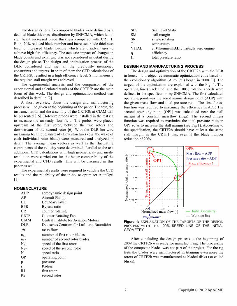
in-house multi-objective automatic optimization code based on the evolutionary algorithm (AutoOpti) began in 2008 [3]. The targets of the optimization are explained with the Fig. 1. The operating line (black line) and the 100% rotation speeds were defined in the specification by SNECMA. The first calculated operating point was the aerodynamic design point (ADP) with the given mass flow and total pressure ratio. The first fitness function was required to maximize the efficiency in ADP. The second operating point (OP1) was calculated near the stall margin at a constant massflow (mSM). The second fitness function was required to maximize the total pressure ratio in OP1 so as to increase the stall margin (see Fig.1). According to the specification, the CRTF2b should have at least the same stall margin as the CRTF1 has, even if the blade number reduction of 20%.

OP0:Mass flow – ADPPressure ratio – ADP! Max. efficiency !

To in

crea

seth

est

all m

argi

n

mSM=konst

Initial GeometryWorking line

OP1

Nor

mal

ized

tota

l pre

ssur

era

tio[-

]

Normalized mass flow [-]

Figure 1: EXPLANATION OF THE TARGETS OF THE DESIGN PROCESS WITH THE 100% SPEED LINE OF THE INITIAL GEOMETRY

After concluding the design process at the beginning of

2009 the CRTF2b was ready for manufacturing. The processing of the composite blades was not part of the project. For the rig tests the blades were manufactured in titanium even more the rotors of CRTF2b was manufactured as bladed disks (so called blisks).


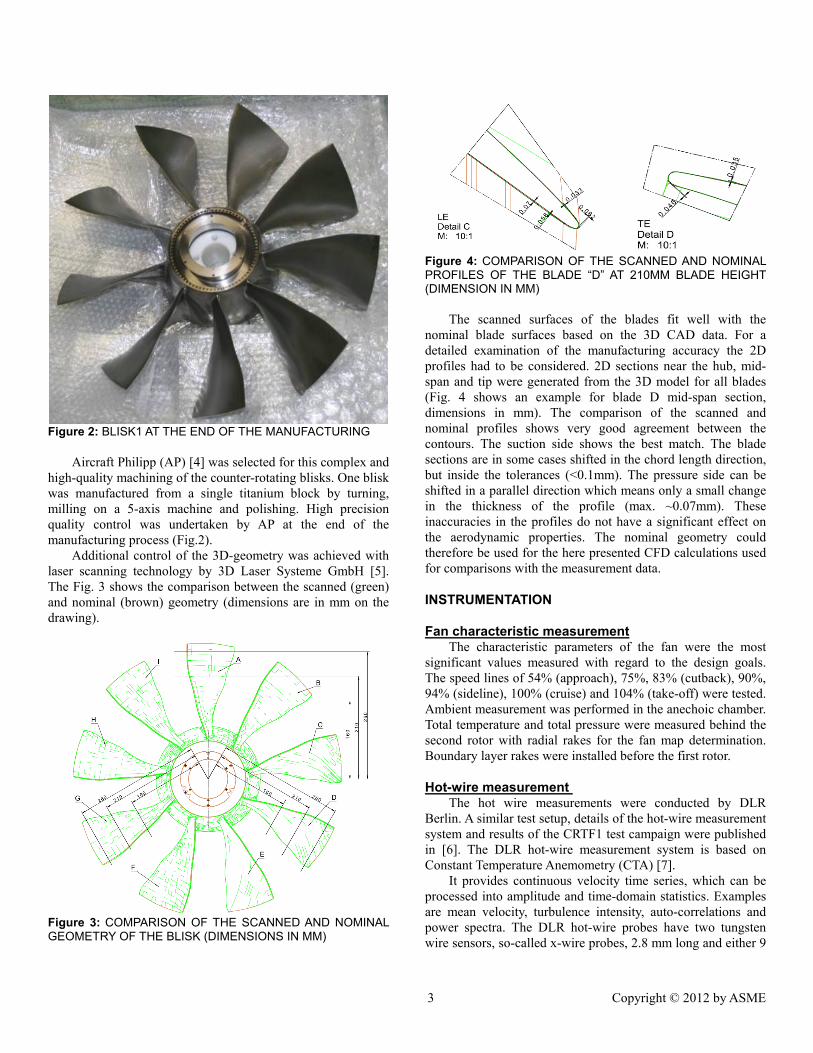
Figure 2: BLISK1 AT THE END OF THE MANUFACTURING

Aircraft Philipp (AP) [4] was selected for this complex and high-quality machining of the counter-rotating blisks. One blisk was manufactured from a single titanium block by turning, milling on a 5-axis machine and polishing. High precision quality control was undertaken by AP at the end of the manufacturing process (Fig.2).

Additional control of the 3D-geometry was achieved with laser scanning technology by 3D Laser Systeme GmbH [5]. The Fig. 3 shows the comparison between the scanned (green) and nominal (brown) geometry (dimensions are in mm on the drawing).

Figure 3: COMPARISON OF THE SCANNED AND NOMINAL GEOMETRY OF THE BLISK (DIMENSIONS IN MM)

Figure 4: COMPARISON OF THE SCANNED AND NOMINAL PROFILES OF THE BLADE “D” AT 210MM BLADE HEIGHT (DIMENSION IN MM)

The scanned surfaces of the blades fit well with the

nominal blade surfaces based on the 3D CAD data. For a detailed examination of the manufacturing accuracy the 2D profiles had to be considered. 2D sections near the hub, mid-span and tip were generated from the 3D model for all blades (Fig. 4 shows an example for blade D mid-span section, dimensions in mm). The comparison of the scanned and nominal profiles shows very good agreement between the contours. The suction side shows the best match. The blade sections are in some cases shifted in the chord length direction, but inside the tolerances (<0.1mm). The pressure side can be shifted in a parallel direction which means only a small change in the thickness of the profile (max. ~0.07mm). These inaccuracies in the profiles do not have a significant effect on the aerodynamic properties. The nominal geometry could therefore be used for the here presented CFD calculations used for comparisons with the measurement data.

INSTRUMENTATION

Fan characteristic measurement The characteristic parameters of the fan were the most

significant values measured with regard to the design goals. The speed lines of 54% (approach), 75%, 83% (cutback), 90%, 94% (sideline), 100% (cruise) and 104% (take-off) were tested. Ambient measurement was performed in the anechoic chamber. Total temperature and total pressure were measured behind the second rotor with radial rakes for the fan map determination. Boundary layer rakes were installed before the first rotor.

Hot-wire measurement The hot wire measurements were conducted by DLR

Berlin. A similar test setup, details of the hot-wire measurement system and results of the CRTF1 test campaign were published in [6]. The DLR hot-wire measurement system is based on Constant Temperature Anemometry (CTA) [7].

It provides continuous velocity time series, which can be processed into amplitude and time-domain statistics. Examples are mean velocity, turbulence intensity, auto-correlations and power spectra. The DLR hot-wire probes have two tungsten wire sensors, so-called x-wire probes, 2.8 mm long and either 9


or 12.5 µm diameter, each mounted on two needle-shaped prongs. This allows the measurement of two velocity components (axial and radial or axial and circumferential) at each probe position.

This measuring technique was applied for the examination of the unsteady behavior of the counter rotating fan particularly with regard to the R1 wakes and the upstream effects of R2 in a plane between the rotors at three operating points. Hot-wire probes (HW) were placed in the contra rotating turbo fan rig upstream of the first rotor, between the rotors and downstream of the second rotor (planes A3, B4 and D1 in Figure 10). Hot-wire probes HW 1 (plane A3) and HW 4 (plane D1) were adjusted in a fixed radial position (50 mm from outer casing). The first one was installed to measure the turbulent intensity which was an important inlet boundary condition for the CFD calculation. The two hot-wire probes HW 2 and HW 3 (plane B4) were mounted on two radial traverses to allow the adjustment of different radial distances. This allowed determination of the velocity flow field with axial, radial and circumferential components in this plane. Since only x-wire probes (with only two wires inclined by about 90° on each probe) were used, two probes were needed to capture the three components of the velocity vector. The immersion distance of these probes was varied between 10 mm and 118 mm from the outer annulus line (roughly 95%-40% of the relative channel height). 11 radial positions for each operating point have in total been measured. The two traverses were placed at the same axial but different circumferential position. The circumferential displacement is exactly one blade pitch of R1.

The sampling rate of the data acquisition is 192 kHz with 24 bit of resolution. This ensures a measurement accuracy of about 283 measurement points per blade pitch.

To minimize the temperature and Mach-number dependence, the hot-wire calibration was made using dimensionless Reynolds and Nusselt numbers [6], instead of voltage and velocity. Therefore, the temperature also has to be measured in each plane during the test.

In parallel with the hot-wire signals the trigger signals (1/ref) of both rotors were recorded. The determination of the mean velocities and the turbulence levels as well as the spectral analysis requires a phase-locked averaging technique based on a detailed rotor trigger interpretation.

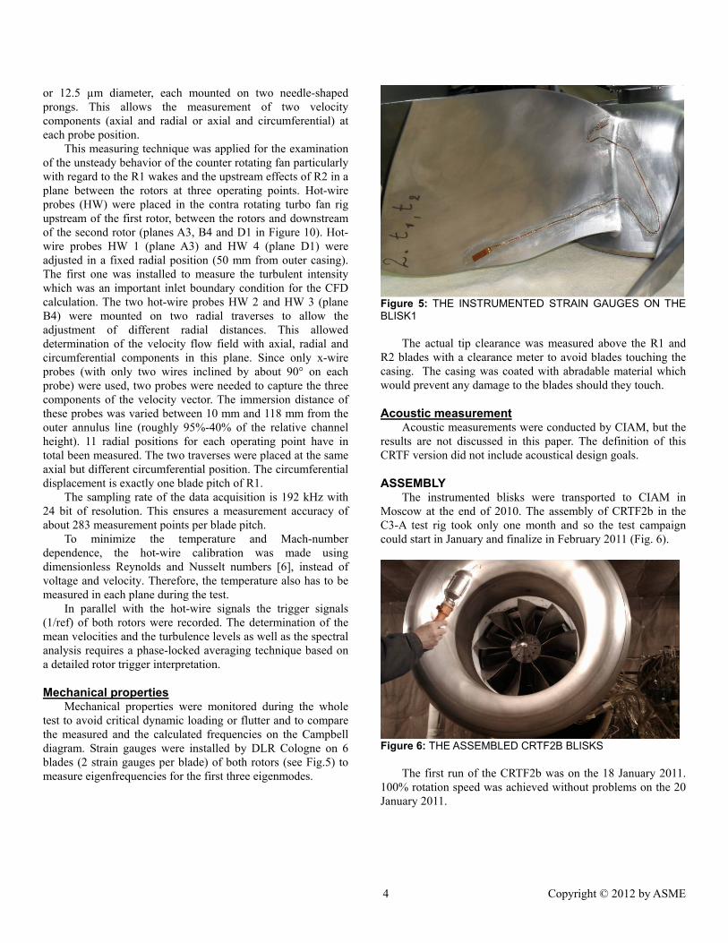
Mechanical properties Mechanical properties were monitored during the whole

test to avoid critical dynamic loading or flutter and to compare the measured and the calculated frequencies on the Campbell diagram. Strain gauges were installed by DLR Cologne on 6 blades (2 strain gauges per blade) of both rotors (see Fig.5) to measure eigenfrequencies for the first three eigenmodes.

Figure 5: THE INSTRUMENTED STRAIN GAUGES ON THE BLISK1

The actual tip clearance was measured above the R1 and R2 blades with a clearance meter to avoid blades touching the casing. The casing was coated with abradable material which would prevent any damage to the blades should they touch.

Acoustic measurement Acoustic measurements were conducted by CIAM, but the

results are not discussed in this paper. The definition of this CRTF version did not include acoustical design goals.

ASSEMBLY The instrumented blisks were transported to CIAM in

Moscow at the end of 2010. The assembly of CRTF2b in the C3-A test rig took only one month and so the test campaign could start in January and finalize in February 2011 (Fig. 6).

Figure 6: THE ASSEMBLED CRTF2B BLISKS

The first run of the CRTF2b was on the 18 January 2011. 100% rotation speed was achieved without problems on the 20 January 2011.


HIGH-RESOLUTION CFD CALCULATION FOR THE COMPARISON

The process of design through the automatic optimizer required a simple calculation domain with a coarse mesh to allow parametric geometry generation, meshing and to save calculation time [1][3]. This mesh was not adequate for a detailed comparison with measurement results. An extended calculation domain, with a high-resolution mesh, was therefore generated to make the comparison.

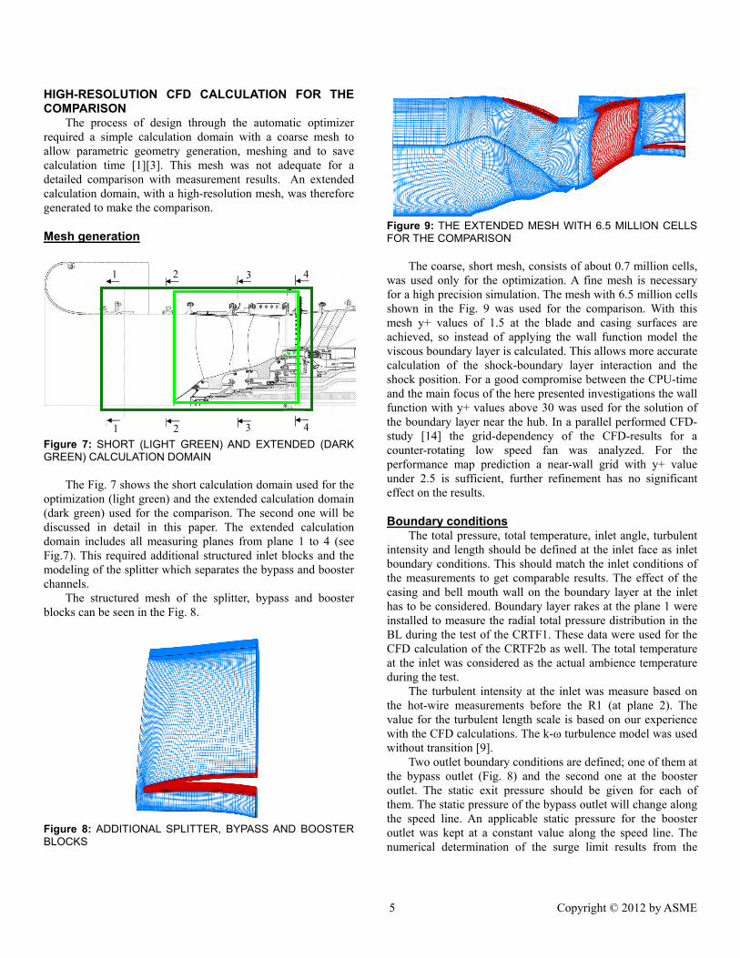
Mesh generation

Figure 7: SHORT (LIGHT GREEN) AND EXTENDED (DARK GREEN) CALCULATION DOMAIN

The Fig. 7 shows the short calculation domain used for the optimization (light green) and the extended calculation domain (dark green) used for the comparison. The second one will be discussed in detail in this paper. The extended calculation domain includes all measuring planes from plane 1 to 4 (see Fig.7). This required additional structured inlet blocks and the modeling of the splitter which separates the bypass and booster channels.

The structured mesh of the splitter, bypass and booster blocks can be seen in the Fig. 8.

Figure 8: ADDITIONAL SPLITTER, BYPASS AND BOOSTER BLOCKS

Figure 9: THE EXTENDED MESH WITH 6.5 MILLION CELLS FOR THE COMPARISON

The coarse, short mesh, consists of about 0.7 million cells,

was used only for the optimization. A fine mesh is necessary for a high precision simulation. The mesh with 6.5 million cells shown in the Fig. 9 was used for the comparison. With this mesh y+ values of 1.5 at the blade and casing surfaces are achieved, so instead of applying the wall function model the viscous boundary layer is calculated. This allows more accurate calculation of the shock-boundary layer interaction and the shock position. For a good compromise between the CPU-time and the main focus of the here presented investigations the wall function with y+ values above 30 was used for the solution of the boundary layer near the hub. In a parallel performed CFD-study [14] the grid-dependency of the CFD-results for a counter-rotating low speed fan was analyzed. For the performance map prediction a near-wall grid with y+ value under 2.5 is sufficient, further refinement has no significant effect on the results.

Boundary conditions The total pressure, total temperature, inlet angle, turbulent

intensity and length should be defined at the inlet face as inlet boundary conditions. This should match the inlet conditions of the measurements to get comparable results. The effect of the casing and bell mouth wall on the boundary layer at the inlet has to be considered. Boundary layer rakes at the plane 1 were installed to measure the radial total pressure distribution in the BL during the test of the CRTF1. These data were used for the CFD calculation of the CRTF2b as well. The total temperature at the inlet was considered as the actual ambience temperature during the test.

The turbulent intensity at the inlet was measure based on the hot-wire measurements before the R1 (at plane 2). The value for the turbulent length scale is based on our experience with the CFD calculations. The k-ω turbulence model was used without transition [9].

Two outlet boundary conditions are defined; one of them at the bypass outlet (Fig. 8) and the second one at the booster outlet. The static exit pressure should be given for each of them. The static pressure of the bypass outlet will change along the speed line. An applicable static pressure for the booster outlet was kept at a constant value along the speed line. The numerical determination of the surge limit results from the

1

1

2

2

3

3

4

4


increase of the static pressure at the bypass outlet in small steps. The limit was detected by a non-convergence calculation.

Tip clearance A nominal hot tip clearance of 0.36 mm for R1 and 0.28

mm for R2 was taken into account for the calculations, because the measured values were not available at the time of the CFD calculations.

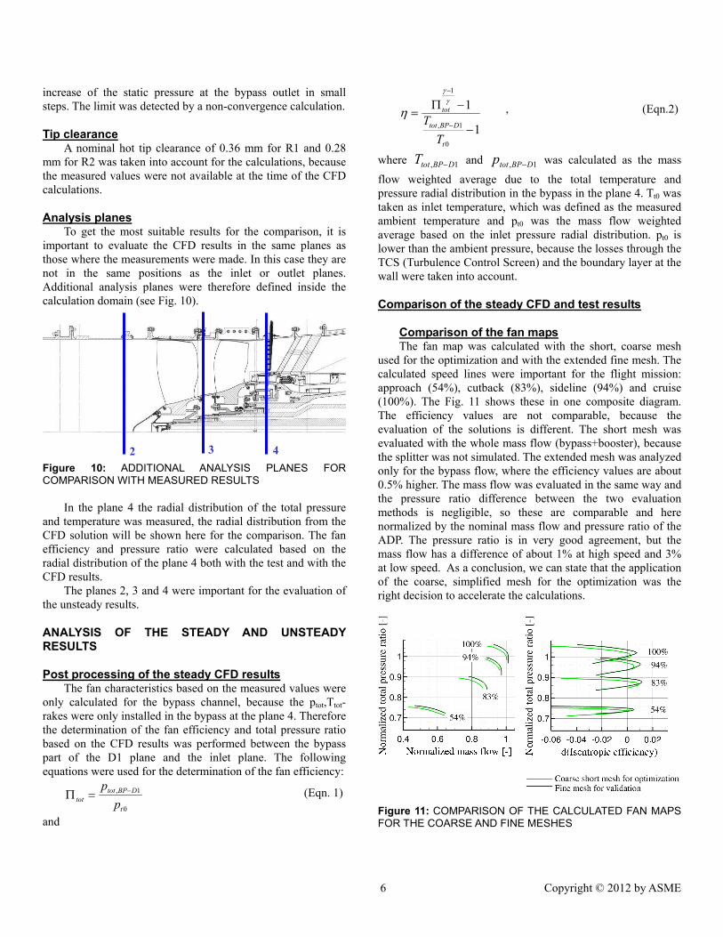
Analysis planes To get the most suitable results for the comparison, it is

important to evaluate the CFD results in the same planes as those where the measurements were made. In this case they are not in the same positions as the inlet or outlet planes. Additional analysis planes were therefore defined inside the calculation domain (see Fig. 10).

Figure 10: ADDITIONAL ANALYSIS PLANES FOR COMPARISON WITH MEASURED RESULTS

In the plane 4 the radial distribution of the total pressure and temperature was measured, the radial distribution from the CFD solution will be shown here for the comparison. The fan efficiency and pressure ratio were calculated based on the radial distribution of the plane 4 both with the test and with the CFD results.

The planes 2, 3 and 4 were important for the evaluation of the unsteady results.

ANALYSIS OF THE STEADY AND UNSTEADY RESULTS

Post processing of the steady CFD results The fan characteristics based on the measured values were

only calculated for the bypass channel, because the ptot,Ttot-rakes were only installed in the bypass at the plane 4. Therefore the determination of the fan efficiency and total pressure ratio based on the CFD results was performed between the bypass part of the D1 plane and the inlet plane. The following equations were used for the determination of the fan efficiency:

0

1,

t

DBPtottot p

p −=Π (Eqn. 1)

and

1

1

0

1,

1

−

−Π=

−

−

t

DBPtot

tot

TT

γγ

η , (Eqn.2)

where 1, DBPtotT − and 1, DBPtotp − was calculated as the mass

flow weighted average due to the total temperature and pressure radial distribution in the bypass in the plane 4. Tt0 was taken as inlet temperature, which was defined as the measured ambient temperature and pt0 was the mass flow weighted average based on the inlet pressure radial distribution. pt0 is lower than the ambient pressure, because the losses through the TCS (Turbulence Control Screen) and the boundary layer at the wall were taken into account.

Comparison of the steady CFD and test results

Comparison of the fan maps The fan map was calculated with the short, coarse mesh

used for the optimization and with the extended fine mesh. The calculated speed lines were important for the flight mission: approach (54%), cutback (83%), sideline (94%) and cruise (100%). The Fig. 11 shows these in one composite diagram. The efficiency values are not comparable, because the evaluation of the solutions is different. The short mesh was evaluated with the whole mass flow (bypass+booster), because the splitter was not simulated. The extended mesh was analyzed only for the bypass flow, where the efficiency values are about 0.5% higher. The mass flow was evaluated in the same way and the pressure ratio difference between the two evaluation methods is negligible, so these are comparable and here normalized by the nominal mass flow and pressure ratio of the ADP. The pressure ratio is in very good agreement, but the mass flow has a difference of about 1% at high speed and 3% at low speed. As a conclusion, we can state that the application of the coarse, simplified mesh for the optimization was the right decision to accelerate the calculations.

Figure 11: COMPARISON OF THE CALCULATED FAN MAPS FOR THE COARSE AND FINE MESHES

4 2 3


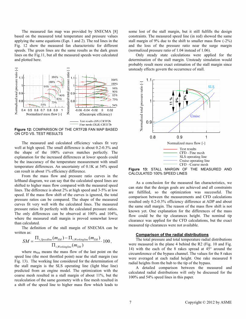
The measured fan map was provided by SNECMA [8] based on the measured total temperature and pressure values applying the same equations (Eqn. 1 and 2). The red lines in the Fig. 12 show the measured fan characteristic for different speeds. The green lines are the same results as the dark green lines on the Fig.11, but all the measured speeds were calculated and plotted here.

Figure 12: COMPARISON OF THE CRTF2B FAN MAP BASED ON CFD VS. TEST RESULTS

The measured and calculated efficiency values fit very well at high speed. The small difference is about 0.2-0.3% and the shape of the 100% curves matches perfectly. The explanation for the increased differences at lower speeds could be the inaccuracy of the temperature measurement with small temperature differences. An uncertainty of 0.1K at 54% speed can result in about 1% efficiency difference.

From the mass flow and pressure ratio curves in the lefthand diagram, we can say that the calculated speed lines are shifted to higher mass flow compared with the measured speed lines. The difference is about 2% at high speed and 3-5% at low speed. If the mass flow shift of the curves is ignored, the total pressure ratios can be compared. The shape of the measured curves fit very well with the calculated lines. The measured pressure ratios fit perfectly with the calculated pressure ratios. The only differences can be observed at 100% and 104%, where the measured stall margin is proved somewhat lower than calculated.

The definition of the stall margin of SNECMA can be written as:

100)(

)()(

,

,, ⋅Π

Π−Π=

SMeWorkinglint

SMeWorkinglintSMSpeedlinet

mmm

SM ,

where mSM means the mass flow of the last point on the speed line (the most throttled point) near the stall margin (see Fig. 13). The working line considered for the determination of the stall margin is the SLS operating line (light blue line) predicted from an engine model. The optimization with the coarse mesh resulted in a stall margin of about 11%, but the recalculation of the same geometry with a fine mesh resulted in a shift of the speed line to higher mass flow which leads to

some lost of the stall margin, but it still fulfills the design constraints. The measured speed line (in red) showed the same stall margin of 9% due to the shift to smaller mass flow (-2%) and the loss of the pressure ratio near the surge margin (normalized pressure ratio of 1.04 instead of 1.06).

Only steady state calculations were applied for the determination of the stall margin. Unsteady simulation would probably result more exact estimation of the stall margin since unsteady effects govern the occurrence of stall.

Figure 13: STALL MARGIN OF THE MEASURED AND CALCULATED 100% SPEED LINES

As a conclusion for the measured fan characteristics, we can state that the design goals are achieved and all constraints are fulfilled, so the optimization was successful. The comparison between the measurements and CFD calculations resulted only 0.2-0.3% efficiency difference at ADP and about the same stall margin. The reason of the mass flow shift is not known yet. One explanation for the differences of the mass flow could be the tip clearances height. The nominal tip clearance was applied for the CFD calculations, but the exact measured tip clearances were not available.

Comparison of the radial distributions The total pressure and total temperature radial distributions

were measured in the plane 4 behind the R2 (Fig. 10 and Fig. 14) with the each of the 8 rakes spread at 45° around the circumference of the bypass channel. The values for the 8 rakes were averaged at each radial height. One rake measured 8 radial heights from the hub to the tip of the bypass.

A detailed comparison between the measured and calculated radial distributions will only be discussed for the 100% and 54% speed lines in this paper.


Figure 14: INSTRUMENTATION OF PLANE 4 WITH THE RADIAL PT/TT RAKES

100% speed line (Figures 15-19) The measured radial distribution from ‘a’ to ‘d’ and the

increase of the total pressure (Fig. 16 left side) and temperature (Fig. 16 right side) can be observed. This is due to the fact that the curve ‘a’ is in choked condition and the throttling was increased from the point ‘a’ to ‘e’. The behavior of the curve ‘e’ is changed; the pt near the tip and the Tt along the blade height decreased compared to point ‘d’. The increased exit static pressure can not provide higher total pressure for the point ‘e’, so the pressure ratio curve on Fig.15 has broken down at point ‘e’. This indicates an operating point close to the surge limit for the measured speed line.

The right hand diagram in Fig. 16 shows the radial distribution of the total temperature at the exit plane (4). Very good agreement can be observed between the temperature gradients; the measured curves run parallel to the calculated curves (except of OP ‘e’).

One measured operating point (‘c’) was selected in Fig. 17 and compared with the equivalent calculated points (‘3’ or ‘4’). The pressure distribution of ‘c’ is fitted to the calculated point ‘3’ and the temperature distribution lies near the curve ‘3’. The differences are about 1-2K. If the accuracy of the applied thermoelements of about 1K is taken into account, we can say, that the results are outstanding. The averaged pressure ratio and efficiency of the operating point ‘c’ matches much better with the calculated point ‘4’.

Figure 15: THE SELECTED OPERATING POINTS FOR THE COMPARISON OF THE RADIAL DISTRIBUTIONS

Figure 16: THE RADIAL DISTRIBUTIONS OF THE TOTAL PRESSURE AND TEMPERATURE

Figure 17: THE RADIAL DISTRIBUTION OF THE TOTAL PRESSURE AND TEMPERATURE FOR 1 MEASURED POINT

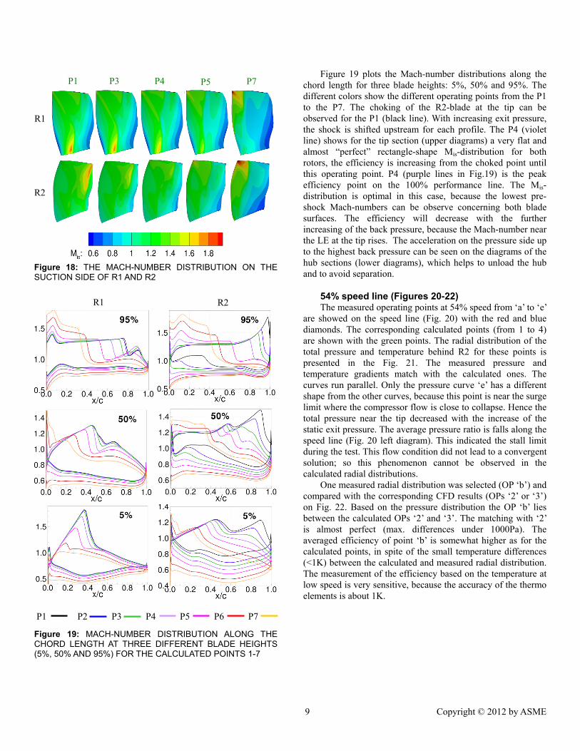
The Mach-number distribution on the suction side of both blades is shown for 5 calculated operating points (1,3,4,5,7) in the Fig. 18. The exit static pressure increases from left to right. The point Nr.7 is the last converged calculated point. The point Nr. 4 has the maximum efficiency.

ΔTt

5K

Test (Test)

10000Pa

Δpt

Test CFD

Δpt ΔTt

5K 10000Pa

CFD


Figure 18: THE MACH-NUMBER DISTRIBUTION ON THE SUCTION SIDE OF R1 AND R2

Figure 19: MACH-NUMBER DISTRIBUTION ALONG THE CHORD LENGTH AT THREE DIFFERENT BLADE HEIGHTS (5%, 50% AND 95%) FOR THE CALCULATED POINTS 1-7

Figure 19 plots the Mach-number distributions along the chord length for three blade heights: 5%, 50% and 95%. The different colors show the different operating points from the P1 to the P7. The choking of the R2-blade at the tip can be observed for the P1 (black line). With increasing exit pressure, the shock is shifted upstream for each profile. The P4 (violet line) shows for the tip section (upper diagrams) a very flat and almost “perfect” rectangle-shape Mis-distribution for both rotors, the efficiency is increasing from the choked point until this operating point. P4 (purple lines in Fig.19) is the peak efficiency point on the 100% performance line. The Mis-distribution is optimal in this case, because the lowest pre-shock Mach-numbers can be observe concerning both blade surfaces. The efficiency will decrease with the further increasing of the back pressure, because the Mach-number near the LE at the tip rises. The acceleration on the pressure side up to the highest back pressure can be seen on the diagrams of the hub sections (lower diagrams), which helps to unload the hub and to avoid separation.

54% speed line (Figures 20-22) The measured operating points at 54% speed from ‘a’ to ‘e’

are showed on the speed line (Fig. 20) with the red and blue diamonds. The corresponding calculated points (from 1 to 4) are shown with the green points. The radial distribution of the total pressure and temperature behind R2 for these points is presented in the Fig. 21. The measured pressure and temperature gradients match with the calculated ones. The curves run parallel. Only the pressure curve ‘e’ has a different shape from the other curves, because this point is near the surge limit where the compressor flow is close to collapse. Hence the total pressure near the tip decreased with the increase of the static exit pressure. The average pressure ratio is falls along the speed line (Fig. 20 left diagram). This indicated the stall limit during the test. This flow condition did not lead to a convergent solution; so this phenomenon cannot be observed in the calculated radial distributions.

One measured radial distribution was selected (OP ‘b’) and compared with the corresponding CFD results (OPs ‘2’ or ‘3’) on Fig. 22. Based on the pressure distribution the OP ‘b’ lies between the calculated OPs ‘2’ and ‘3’. The matching with ‘2’ is almost perfect (max. differences under 1000Pa). The averaged efficiency of point ‘b’ is somewhat higher as for the calculated points, in spite of the small temperature differences (<1K) between the calculated and measured radial distribution. The measurement of the efficiency based on the temperature at low speed is very sensitive, because the accuracy of the thermo elements is about 1K.

R1

R2

P1 P3 P4 P5 P7

P1 P2 P3 P4 P5 P6 P7

R2 R1


Figure 20: THE SELECTED OPERATING POINTS FOR COMPARISON OF THE RADIAL DISTRIBUTIONS

Figure 21: THE RADIAL DISTRIBUTIONS OF THE TOTAL PRESSURE AND TEMPERATURE

Figure 22: THE RADIAL DISTRIBUTION OF THE TOTAL PRESSURE AND TEMPERATURE FOR 1 MEASURED POINT

Evaluation of the time-dependent hot-wire results The measurements were conducted under six different

operating conditions at three different main rotor speeds of the compressor fan stage. These conditions are relevant to noise issues for the whole engine. The rotor speeds were adjusted for the approach (54%), cutback (83%) and sideline (94%) cases.

All data shown in this paper were measured at 54% rotor speeds with the baseline nozzle configuration. Fig. 23 shows an example of the axial velocity (U-component) signal at the HW 2 probe downstream of R1 in a mid-span position (80 mm from outer casing). The blue curve shows the instantaneous velocity for one rotation. The wake flow of each blade differs clearly from blade to blade. In contrast to the blue curve, the red curve shows the result of the phase-locked averaged mean velocity for each individual blade, calculated from about 13,680

rotations. The averaged values show very homogeneous behavior. For the averaged values the minimum velocity in the wake of each blade is about ∆U=24 m/s. For the instantaneous velocity this deficit varies in the range of 18 m/s < ΔU < 33 m/s.

Figure 23: UNSTEADY (BLUE) AND PHASE-LOCKED AVERAGED AXIAL MEAN VELOCITY (RED) DOWNSTREAM OF R1 AND 51% BLADE HEIGHT (80 MM FROM OUTER CASING)

Figure 24: AXIAL MEAN FLOW VELOCITY COMPONENT U DOWNSTREAM OF R1 CORRELATED WITH R1 REVOLUTION COUNTER (BLUE: LOW VELOCITY VALUES DUE TO THE WAKE FLOW OF THE R1 BLADES; RED: HIGH VELOCITY VALUES), REARWARD VIEW

If these time series are arranged in a circumferential

direction on the corresponding radial position, the following contour plot can be generated for each velocity component. The phase lock averaging method can be applied for R1 or R2. Figure 24 shows the axial mean flow velocity U downstream of R1. Here the averaging is performed by keeping the phase-locked with respect to the R1 revolution counter. Downstream

ΔTt

1K

Test 5000Pa

Δpt

CFD

ΔTt

2K

Test (Test) 5000Pa

Δpt

CFD


of each blade of R1, a velocity deficit (wake flow), due to flow losses, can be observed. At mid-span stream these losses are dominated by the blade-profile losses. Close to the outer casing, additional losses due to the leakage flow of the blade-tip gap can be seen.

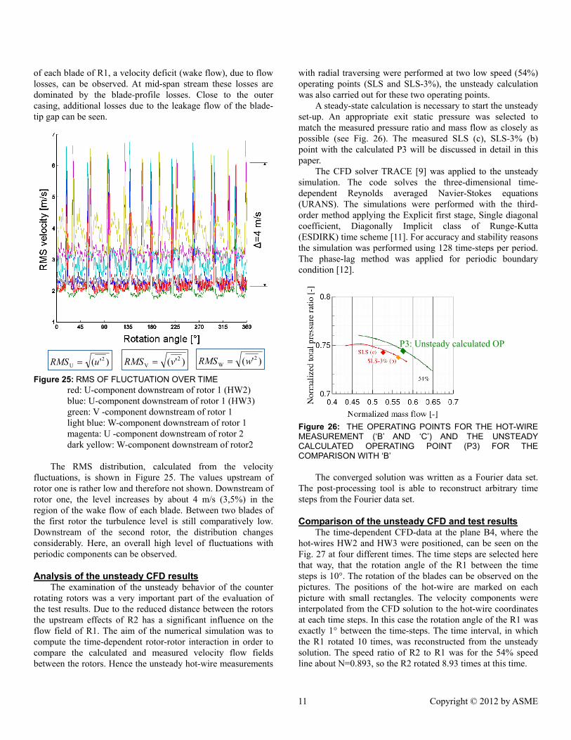
Figure 25: RMS OF FLUCTUATION OVER TIME

red: U-component downstream of rotor 1 (HW2) blue: U-component downstream of rotor 1 (HW3) green: V -component downstream of rotor 1 light blue: W-component downstream of rotor 1 magenta: U -component downstream of rotor 2 dark yellow: W-component downstream of rotor2

The RMS distribution, calculated from the velocity

fluctuations, is shown in Figure 25. The values upstream of rotor one is rather low and therefore not shown. Downstream of rotor one, the level increases by about 4 m/s (3,5%) in the region of the wake flow of each blade. Between two blades of the first rotor the turbulence level is still comparatively low. Downstream of the second rotor, the distribution changes considerably. Here, an overall high level of fluctuations with periodic components can be observed.

Analysis of the unsteady CFD results The examination of the unsteady behavior of the counter

rotating rotors was a very important part of the evaluation of the test results. Due to the reduced distance between the rotors the upstream effects of R2 has a significant influence on the flow field of R1. The aim of the numerical simulation was to compute the time-dependent rotor-rotor interaction in order to compare the calculated and measured velocity flow fields between the rotors. Hence the unsteady hot-wire measurements

with radial traversing were performed at two low speed (54%) operating points (SLS and SLS-3%), the unsteady calculation was also carried out for these two operating points.

A steady-state calculation is necessary to start the unsteady set-up. An appropriate exit static pressure was selected to match the measured pressure ratio and mass flow as closely as possible (see Fig. 26). The measured SLS (c), SLS-3% (b) point with the calculated P3 will be discussed in detail in this paper.

The CFD solver TRACE [9] was applied to the unsteady simulation. The code solves the three-dimensional time-dependent Reynolds averaged Navier-Stokes equations (URANS). The simulations were performed with the third-order method applying the Explicit first stage, Single diagonal coefficient, Diagonally Implicit class of Runge-Kutta (ESDIRK) time scheme [11]. For accuracy and stability reasons the simulation was performed using 128 time-steps per period. The phase-lag method was applied for periodic boundary condition [12].

Figure 26: THE OPERATING POINTS FOR THE HOT-WIRE MEASUREMENT (‘B’ AND ‘C’) AND THE UNSTEADY CALCULATED OPERATING POINT (P3) FOR THE COMPARISON WITH ‘B’

The converged solution was written as a Fourier data set. The post-processing tool is able to reconstruct arbitrary time steps from the Fourier data set.

Comparison of the unsteady CFD and test results The time-dependent CFD-data at the plane B4, where the

hot-wires HW2 and HW3 were positioned, can be seen on the Fig. 27 at four different times. The time steps are selected here that way, that the rotation angle of the R1 between the time steps is 10°. The rotation of the blades can be observed on the pictures. The positions of the hot-wire are marked on each picture with small rectangles. The velocity components were interpolated from the CFD solution to the hot-wire coordinates at each time steps. In this case the rotation angle of the R1 was exactly 1° between the time-steps. The time interval, in which the R1 rotated 10 times, was reconstructed from the unsteady solution. The speed ratio of R2 to R1 was for the 54% speed line about N=0.893, so the R2 rotated 8.93 times at this time.

)'( 2V vRMS =)'( 2

U uRMS = )'( 2W wRMS =

P3: Unsteady calculated OP


The axial velocity components at mid-span (r8) position for the 11 R1-rotations are monitored on the Fig. 28. The wakes of the R1-blades and the upstream effects of the R2-blades can be clearly seen. The periodicity of 440° results from the number of blades and speed ratio. R2 is rotating at this time °=⋅°=⋅°= 9.392893.04404402 NRα . The R1 includes nR1=9 blades, so one pitch is 360°/9=40°. The R2 includes nR2=11 blades, so one pitch is 360°/11=32.73°. While R1 is rotating 440°, during this time 440°/40°=11 pitch of R1 is passed before the hot-wires and 392.9°/32.73=12.00 pitch of R2 is passed behind the hot-wire. This phenomenon can explain the periodicity at 54% speed line. The speed ratio has a very significant influence on the periodicity. A small change of the speed ratio can result in a completely different periodicity. Due to this example, a periodicity of two counter rotating rotors can exist, if there are p1 and p2 integers without common diviser, with them:

2

1

2

1

2

1

nn

NN

pp

⋅= (3)

where p1 is the number of the R1-pitches in one period and p2 is the number of R2-pitches in one period. In this case: p1=11 and p2=12. In the most cases p will be much higher. This speed ratio and blade number composition is a special case.

Figure 27: VELOCITY VALUE INTERPOLATION ON THE HOT WIRE POSITIONS (FORWARD VIEW)

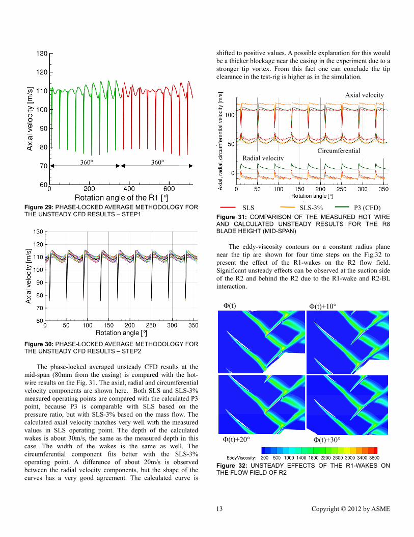
To compare the velocity components calculated and measured, the determination of the phase-locked averaged velocity is necessary. Due to the phase-locked averaging method of the hot-wire results, the time steps with a difference of 360° had to be averaged. The Fig. 29 shows an example for the first (green) and second (red) R1-rotation. The red values were shifted with -360°, so the first and second rotations were lying upon each other. This process was repeated for all eleven rotations until all rotations are positioned from 0° to 360°. The resulted graph can be seen on the Fig. 30 with the different colour curves. Each colour means an other rotation. The 11 curves can be now averaged. The result is shown by the black curve.

The upstream effect of the R2-blades can be clearly seen on the Fig. 27-29. Maximal ±5 m/s velocity fluctuation was observed due to this effect. Eleven velocity peaks can be seen on the full annulus contour plots (Fig. 27) corresponding the number of the R2-blades. The shape of the velocity-curve between the wakes are all different inside one rotation, because the relative position of the R1 and R2 blades is different in each pitch. The shape of the velocity curve repeats after the periodicity of 440° (11 R1-pitch). The upstream-effect of the R2 is therefore wiped out by the R1-based phase-locked averaging method. Each pitch of the averaged (black) curve on the Fig. 30 seems to be the same.

Figure 28: INTERPOLATED AXIAL VELOCITY ON THE R8 (MID-SPAN) HEIGHT

440° 440° 440° 440°

440°

r8 position Φ(t) Φ(t)+10°

Φ(t)+20° Φ(t)+30°

Hot-wire positions


Figure 29: PHASE-LOCKED AVERAGE METHODOLOGY FOR THE UNSTEADY CFD RESULTS – STEP1

Figure 30: PHASE-LOCKED AVERAGE METHODOLOGY FOR THE UNSTEADY CFD RESULTS – STEP2

The phase-locked averaged unsteady CFD results at the mid-span (80mm from the casing) is compared with the hot-wire results on the Fig. 31. The axial, radial and circumferential velocity components are shown here. Both SLS and SLS-3% measured operating points are compared with the calculated P3 point, because P3 is comparable with SLS based on the pressure ratio, but with SLS-3% based on the mass flow. The calculated axial velocity matches very well with the measured values in SLS operating point. The depth of the calculated wakes is about 30m/s, the same as the measured depth in this case. The width of the wakes is the same as well. The circumferential component fits better with the SLS-3% operating point. A difference of about 20m/s is observed between the radial velocity components, but the shape of the curves has a very good agreement. The calculated curve is

shifted to positive values. A possible explanation for this would be a thicker blockage near the casing in the experiment due to a stronger tip vortex. From this fact one can conclude the tip clearance in the test-rig is higher as in the simulation.

Figure 31: COMPARISON OF THE MEASURED HOT WIRE AND CALCULATED UNSTEADY RESULTS FOR THE R8 BLADE HEIGHT (MID-SPAN)

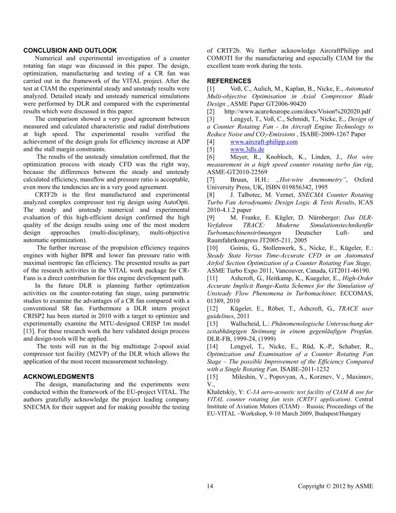
The eddy-viscosity contours on a constant radius plane near the tip are shown for four time steps on the Fig.32 to present the effect of the R1-wakes on the R2 flow field. Significant unsteady effects can be observed at the suction side of the R2 and behind the R2 due to the R1-wake and R2-BL interaction.

Figure 32: UNSTEADY EFFECTS OF THE R1-WAKES ON THE FLOW FIELD OF R2

Φ(t) Φ(t)+10°

Φ(t)+20° Φ(t)+30°

SLS SLS-3% P3 (CFD)

Axial velocity

Circumferential Radial velocity360° 360°


CONCLUSION AND OUTLOOK Numerical and experimental investigation of a counter

rotating fan stage was discussed in this paper. The design, optimization, manufacturing and testing of a CR fan was carried out in the framework of the VITAL project. After the test at CIAM the experimental steady and unsteady results were analyzed. Detailed steady and unsteady numerical simulations were performed by DLR and compared with the experimental results which were discussed in this paper.

The comparison showed a very good agreement between measured and calculated characteristic and radial distributions at high speed. The experimental results verified the achievement of the design goals for efficiency increase at ADP and the stall margin constraints.

The results of the unsteady simulation confirmed, that the optimization process with steady CFD was the right way, because the differences between the steady and unsteady calculated efficiency, massflow and pressure ratio is acceptable, even more the tendencies are in a very good agreement.

CRTF2b is the first manufactured and experimental analyzed complex compressor test rig design using AutoOpti. The steady and unsteady numerical and experimental evaluation of this high-efficient design confirmed the high quality of the design results using one of the most modern design approaches (multi-disciplinary, multi-objective automatic optimization).

The further increase of the propulsion efficiency requires engines with higher BPR and lower fan pressure ratio with maximal isentropic fan efficiency. The presented results as part of the research activities in the VITAL work package for CR-Fans is a direct contribution for this engine development path.

In the future DLR is planning further optimization activities on the counter-rotating fan stage, using parametric studies to examine the advantages of a CR fan compared with a conventional SR fan. Furthermore a DLR intern project CRISP2 has been started in 2010 with a target to optimize and experimentally examine the MTU-designed CRISP 1m model [13]. For these research work the here validated design process and design-tools will be applied.

The tests will run in the big multistage 2-spool axial compressor test facility (M2VP) of the DLR which allows the application of the most recent measurement technology.

ACKNOWLEDGMENTS The design, manufacturing and the experiments were

conducted within the framework of the EU-project VITAL. The authors gratefully acknowledge the project leading company SNECMA for their support and for making possible the testing

of CRTF2b. We further acknowledge AircraftPhilipp and COMOTI for the manufacturing and especially CIAM for the excellent team work during the tests.

REFERENCES [1] Voß, C., Aulich, M., Kaplan, B., Nicke, E., Automated Multi-objective Optimisation in Axial Compressor Blade Design , ASME Paper GT2006-90420 [2] http://www.acare4europe.com/docs/Vision%202020.pdf [3] Lengyel, T., Voß, C., Schmidt, T., Nicke, E., Design of a Counter Rotating Fan - An Aircraft Engine Technology to Reduce Noise and CO2-Emissions , ISABE-2009-1267 Paper [4] www.aircraft-philipp.com [5] www.3dls.de [6] Meyer, R., Knobloch, K., Linden, J., Hot wire measurement in a high speed counter rotating turbo fan rig, ASME-GT2010-22569 [7] Bruun, H.H.: „Hot-wire Anemometry”, Oxford University Press, UK, ISBN 019856342, 1995 [8] J. Talbotec, M. Vernet, SNECMA Counter Rotating Turbo Fan Aerodynamic Design Logic & Tests Results, ICAS 2010-4.1.2 paper [9] M. Franke, E. Kügler, D. Nürnberger: Das DLR-Verfahren TRACE: Moderne Simulationstechnikenfür Turbomaschinenströmungen Deutscher Luft- und Raumfahrtkongress JT2005-211, 2005 [10] Goinis, G., Stollenwerk, S., Nicke, E., Kügeler, E.: Steady State Versus Time-Accurate CFD in an Automated Airfoil Section Optimization of a Counter Rotating Fan Stage, ASME Turbo Expo 2011, Vancouver, Canada, GT2011-46190. [11] Ashcroft, G., Heitkamp, K., Kuegeler, E., High-Order Accurate Implicit Runge-Kutta Schemes for the Simulation of Unsteady Flow Phenomena in Turbomachiner, ECCOMAS, 01389, 2010 [12] Kügeler, E., Röber, T., Ashcroft, G., TRACE user guidelines, 2011 [13] Wallscheid, L.: Phänomenologische Untersuchung der zeitabhängigen Strömung in einem gegenläufigen Propfan. DLR-FB, 1999-24, (1999) [14] Lengyel, T., Nicke, E., Rüd, K.-P., Schaber, R., Optimization and Examination of a Counter Rotating Fan Stage – The possible Improvement of the Efficiency Compared with a Single Rotating Fan. ISABE-2011-1232 [15] Mileshin, V., Popovyan, A., Korznev, V., Maximov, V., Khaletskiy, Y: C-3A aero-acoustic test facility of CIAM & use for VITAL counter rotating fan tests (CRTF1 application). Central Institute of Aviation Motors (CIAM) – Russia; Proceedings of the EU-VITAL –Workshop, 9-10 March 2009, Budapest/Hungary

ASME Paper GT2012-69587 Final 20120210 - DLR Portalelib.dlr.de/85778/1/Paper_GT2012-69587_Final.pdf2...

Documents

Transcript of ASME Paper GT2012-69587 Final 20120210 - DLR Portalelib.dlr.de/85778/1/Paper_GT2012-69587_Final.pdf2...