Asme 125 (Vibration & Acoustic)(1)

Transactionsof the ASME®

EditorLAWRENCE A. BERGMAN

Assistant to the EditorLINDA CONWAY

Past EditorsF. EHRICHT. CONRY

D. J. INMAN

DESIGN ENGINEERING DIVISION

Associate EditorsJ. CUSUMANO „2003…

S. DYKE „2005…G. FLOWERS „2005…

M. I. FRISWELL „2004…J. GINSBERG „2005…

R. P. S. HAN „2003…J. MAIN „2005…. QUINN „2005…

PARKER „2005…. H. TAN „2004…ICKERT „2003…

D ACOUSTICSDIVISION

. KELTIE „2004…OHAYON „2003…

MUNICATIONSd Vice-President

TECHNICAL PAPERS249 Spectrum of High-Frequency Acoustic Noise in Inviscid Liquid-Linear

Approximation for Spherical WavesL. Likhterov and A. Berman

252 Theory on Pitch Noise and Its ApplicationYukio Nakajima

257 Investigation of the Sound Transmission into an Advanced Grid-StiffenedStructure

Jeffrey S. Vipperman, Deyu Li, Ilya Avdeev, and Steven A. Lane

267 Optimal Stiffener Design for Interior Sound Reduction Using a TopologyOptimization Based Approach

Jianhui Luo and Hae Chang Gea

274 New Evaluation Method on Gear Dynamics Using Continuous andDiscrete Wavelet Transforms

Yuji Ohue and Akira Yoshida

282 A Stochastic Model for Simulation and Diagnostics of Rolling ElementBearings With Localized Faults

J. Antoni and R. B. Randall

coelastically

g Volterra

of a

afting

e Gas

ve

ined Beam

Journal of Vibrationand AcousticsPublished Quarterly by The American Society of Mechanical Engineers

VOLUME 125 • NUMBER 3 • JULY 2003

e back cover …

DR.

CJ. W

NOISE CONTROL AN

RR.

BOARD ON COMChair an

OFFICERSPresident, REG

VIR

PUBManaging Dire

THOMA

DirectoPH

MJ

Produ

ProMA

Transactions of the ASME, JournaAcoustics (ISSN 1048-9002)(Jan., April, July, Oct.) by The

Mechanical Engineers, Three Park A10016. Periodicals postage paid

additional mailing offices. POSTMAchanges to Transactions of

Vibration and Acoustics, c/o THE AMEMECHANICAL ENGINEERS, 22

Fairfield, NJ 07007-2300. CHANGES OFreceived at Society headquarters

they are to be eold la

STATEMENT from By-Laws. Thresponsible for statements or opinion

or ... printed in its publicCOPYRIGHT © 2003 by the American S

Engineers. Authorization to phinternal or personal use under circ

within the fair use provisions of the Coby ASME to libraries and otherthe Copyright Clearance Center

Reporting Service provided that thearticle is paid directly to CCC

Danvers, MA 01923. Request for speccopying should be addressed to

Department. INDEXED by Applied MeEngineering Information, Inc.

Services Tax Reg

OZDEN OCHOA

OF THE ASMEINALD VACHON

Exec. DirectorGIL R. CARTER

TreasurerR. E. NICKELL

LISHING STAFFctor, EngineeringS G. LOUGHLIN

r, Technical Publ.ILIP DI VIETRO

anager, JournalsOAN MERANZE

ction CoordinatorRAY RAMONAS

duction AssistantRISOL ANDINO

l of Vibration andis published quarterlyAmerican Society of

venue, New York, NYat New York, NY andSTER: Send addressthe ASME, Journal ofRICAN SOCIETY OFLaw Drive, Box 2300,

ADDRESS must beseven weeks before

ffective. Please sendbel and new address.e Society shall not bes advanced in papersations (B7.1, Par. 3).ociety of Mechanicalotocopy material for

umstances not fallingpyright Act is grantedusers registered with(CCC) Transactional

base fee of $3.00 per, 222 Rosewood Dr.,

ial permission or bulkReprints/Permission

chanics Reviews andCanadian Goods andistration #126148048

290 Nonlinear Dynamic Analysis of a Rotor Shaft System With VisSupported Bearings

Nabeel Shabaneh and Jean W. Zu

299 Nonlinear Parameter Estimation in Rotor-Bearing System UsinSeries and Method of Harmonic Probing

Animesh Chatterjee and Nalinaksh S. Vyas

307 Effect of Thrust Magnetic Bearing on Stability and BifurcationFlexible Rotor Active Magnetic Bearing System

Y. S. Ho, H. Liu, and L. Yu

317 Torsional Vibration Analysis of Complicated Multi-Branched ShSystems by Modal Synthesis Method

Chun-Ping Zou, Duan-Shi Chen, and Hong-Xing Hua

324 Study on the Dynamics of a Rotor in a Maneuvering AircraftFusheng Lin and Guang Meng

328 Control of Self-Excited Vibration of a Rotor System With ActivBearings

Jinhao Qiu, Junji Tani, and Taekyu Kwon

335 Vibration of Flex Circuits in Hard Disk DrivesJ. A. Wickert

343 Vibration Control of a Traveling Suspended System Using WaAbsorbing Control

M. Saigo, K. Tani, and H. Usui

351 Dynamic Stiffness Formulation and Its Application for a Comband a Two Degree-of-Freedom System

J. R. Banerjee

359 Effect of Damping on Asymmetric SystemsPaolo Gallina

„Contents continued on insid

„Contents continued …

Volume 125, Number 3Journal of Vibration and Acoustics JULY 2003

365 The Effect of Actuator and Sensor Placement on the Active Control of Rotor UnbalanceMarty E. Johnson, Luiz P. Nascimento, Mary Kasarda, and Chris R. Fuller

374 Robust Control of a 2D Acoustic EnclosureHemanshu R. Pota, Ian R. Petersen, and Atul G. Kelkar

384 Active Vibration Suppression With Time Delayed FeedbackRifat Sipahi and Nejat Olgac

389 Bayesian Model Screening for the Identification of Nonlinear Mechanical StructuresGaetan Kerschen, Jean-Claude Golinval, and Franc ¸ois M. Hemez

TECHNICAL BRIEFS398 Closed-Form Exact Solution to H` Optimization of Dynamic Vibration Absorbers „Application to Different

Transfer Functions and Damping Systems …

Toshihiko Asami and Osamu Nishihara

405 Determining Stability Boundaries Using Gyroscopic EigenfunctionsAnthony A. Renshaw

407 Rotor Isolation for Vibration and Noise ReductionTimothy A. Brungart and Eric T. Riggs

The ASME Journal of Vibration and Acoustics is abstracted andindexed in the following:Acoustics Abstracts, Aluminum Industry Abstracts, Applied Science & TechnologyIndex, AMR Abstracts Database, Aquatic Science and Fisheries Abstracts, CivilEngineering Abstracts, Compendex (The electronic equivalent of Engineering Index),Corrosion Abstracts, Current Contents, EEA (Earthquake Engineering AbstractsDatabase), Electronics & Communications Abstracts, Engineered Materials Abstracts,Engineering Index, Enviroline (The electronic equivalent of Environment Abstracts),Environment Abstracts, Environmental Engineering Abstracts, Environmental Scienceand Pollution Management, Excerpta Medica, Fluidex, Health & Safety ScienceAbstracts, INSPEC, Materials Science Citation Index, Mechanical & TransportationEngineering Abstracts, Mechanical Engineering Abstracts, METADEX (The electronicequivalent of Metals Abstracts and Alloys Index), Pollution Abstracts, Referativnyi Zhur-nal, Shock & Vibration Digest, Solid State and Superconductivity Abstracts, Steels Alert

L. Likhterov

A. Berman

Institutes for Applied Researchand Dept. of Biotechnology Engineering,

Ben-Gurion University of the Negev,Beer-Sheva, 84105, Israel

Spectrum of High-FrequencyAcoustic Noise in InviscidLiquid-Linear Approximation forSpherical WavesThe high-frequency asymptotics of the acoustic noise spectrum is considered for the caseof spherically symmetric waves propagating in an unbounded inviscid liquid. Using theKirkwood and Bethe hypothesis regarding kinetic enthalpy, the Euler equations, the equa-tion of state in the Tait’s form and following linearization allow the kinetic enthalpy and‘‘reduced’’ pressure to be obtained. The Fourier transform yields the spectral density ofacoustic energy which proves to be inversely proportional to the square frequency anddecreases approximately by 6 decibels per octave with increase of a frequency.@DOI: 10.1115/1.1570446#

1 IntroductionIt is known that the acoustic noise spectrum has some slope in

the high range of frequencies. The typical Knudsen sea-noisespectral slope is about25 decibels per octave@1#, ~see p. 336!.Acoustic noise spectra generated by oscillating bubbles have beenstudied most completely. Analysis of the acoustic energy gener-ated versus frequency@2# suggests that the25 decibels per octavewind dependent ambient noise slopes of the Knudsen curves arecaused by the shorter lifetimes of high-frequency bubbles, ratherthan significantly lower peak pressure. The average of severalacoustic spectra from a single energetic spill was shown a slope of25 decibels per octave over the frequency range up to 8 kHzaccording to the same authors. The experimental data cited byLonguet-Higgins@3# show that deep water bubble noise spectra inhigh-frequency range~over 10 kHz! have the slope of2~5–7!decibels per octave. Pumphrey and Crum@4# have obtained acous-tic power spectra for rain drops falling onto a lake in slightlywindy conditions which have the slope approximately25 deci-bels per octave. In the spacious review by Prosperetti and Oguz@5#, the comparison between measured and computed underwaternoise spectra demonstrates the decrease of sound levels about25.5 decibels per octave. According to Urick@6#, ~see p. 209!, thespectral slope of a spectrum of deep-sea noise is2~5–6! dB/octave in the frequency band from one up to hundred kilohertz,and further, the thermal noise leads to the 6 dB/octave increase ofthe spectrum level. However, such a rise gives the unlimitedacoustic energy (Eac5*0

`Sdv, whereS is the spectral density andv is the frequency!. It is of interest to elucidate analytically theasymptotic behavior of an acoustic spectrum of spherical wavesspreading in unbounded inviscid medium for following compari-son with experimental data.

2 Initial EquationsThe initial system of governing equations is the Navier-Stokes

equations which for inviscid medium are reduced to the Eulerequations~the spherical case is considered and the radial velocityis denotedn r5n omitting the index!:

]n

]t1n

]n

]r52

1

r

]p

]r~ the motion equation! (1)

]r

]t1

2r

rn1r

]n

]r1n

]r

]r50 ~ the continuity equation! (2)

with addition of the Tait’s equation of state for water

p1B

p01B5S r

r0D n

, (3)

whereB5300 MPa'3000 atm andn57.As has been noted by Vogel, Bush and Parlitz@7#, the equation

of state given by Rice and Walsh@8# may be used but this equa-tion can not easily be incorporated into the Gilmore@9# model thathas been developed on the basis of the Kirkwood and Bethe hy-pothesis~limited to ongoing waves! described in the monographby Cole @10#.

Related more rigorous and general results can be obtained forthe radiated pressure from a bubble taking into account the heatconduction in the fluid outside the bubble and the effects of theliquid compressibility@11#. However, the Kirkwood and Bethetheory gives good results and therefore found wide use for study-ing the generation and propagation of shock waves. Beside that, itis assumed that the considered process will be isothermal. In theanalysis that follows, the above-mentioned hypothesis is em-ployed. In terms of the enthalpy,dh5dp/r, the sound speed,c2

5]p/]r, and above-mentioned hypothesis which postulates thatthe kinetic enthalpy propagates in medium with the velocityc1n:

F ]

]t1~c1n!

]

]r GF r S h1n2

2 D G50, (4)

the Euler equations~1! and ~2! can be written according to Cole@10# as

]n

]t1n

]n

]r52

]h

]r, (5)

]n

]r1

2n

r5

1

c02

]h

]t. (6)

It should be noted that Eq.~4! is not an equivalent to@]/]t1(c1n)]/]r #(rw)50, wherew is the flow potential, but its use al-lows the relatively simpler result to be obtained.

According to the Tait’s equation, the enthalpy,h, can be ex-pressed in following form:

Contributed by the Technical Committee on Vibration and Sound for publicationin the JOURNAL OF VIBRATION AND ACOUSTICS. Manuscript received May 2002;Revised February 2003. Associate Editor: R. F. Keltie.

Copyright © 2003 by ASMEJournal of Vibration and Acoustics JULY 2003, Vol. 125 Õ 249

h5c0

n21~p

*n21/n21!, (7)

where c025n/r0(p01B) is the sound speed in undisturbed me-

dium andp* 5p1B/p01B is the ‘‘reduced’’ pressure. The den-sity, r, will then be determined as

r5r0p*1/n . (8)

3 Determination of EnthalpyFrom Eq.~6!, the radial derivative of the velocity is:

]n

]r5

1

c02

]h

]t2

2n

r, (9)

and this expression can be substituted into the motion equation~5!that gives

]n

]t1nF 1

c02

]h

]t2

2n

r G52]h

]r. (10)

Now, differentiating Eq.~10! with respect tor, differentiating thecontinuity equation~6! with respect tot, and subtracting the sec-ond from the first, it follows

F]n

]r G2

2n

c02

]2h

]t]r1

]h

]r1

4

r 2 n25]2h

]r 2 11

c02

]2h

]t2 . (11)

The square of the continuity equation is

F]n

]r G2

24n

r

]n

]r1

4n2

r 2 51

c04 F]h

]t G2

, (12)

and Eq.~11! becomes

1

c04 F]h

]t G2

24n

r

]n

]r1

n

c02

]2h

]t]r1

2

r

]h

]r52

]2h

]r 2 1n

c0

]2h

]t2 .

(13)

Using Eq.~6! once more, Eq.~13! can be rewritten in the follow-ing form:

]2h

]r 2 12

r

]h

]r1

1

c02

]2h

]t2 51

c04 F]h

]t G2

24

r

n

c02

]h

]t2

8n2

r 2 1n

c02

]2h

]t]r,

(14)

where all nonlinear terms are collected in the right-hand part ofthis equation.

The evaluation of the nonlinear terms shows that the first termcontains a multiplierc0

24, the second and fourth terms are propor-tional to c0

21M 21 ~M is the Mach number! and the third termcorresponds to the spherical expansion which can be consideredas sufficiently small at large distances from the source of pertur-bations. Therefore, these terms may be neglected if the linearapproximation is considered, and the linear equation follows fordetermination of the enthalpy:

]2h

]r 2 12

r

]h

]r1

1

c02

]2h

]t2 50. (15)

Assumingh5A(r )e2vt, whereA is a function ofr only, theequation for determination ofA(r ) is obtained:

d2A

dr2 12

r

dA

dr1k2A50, (16)

wherek5v/c0 .Multiplying this equation byr, this equation~connected with

the Bessel’s equation! becomes:

rA912A81k2rA50. (17)

According to the formula~2.101! from the handbook of Kamke@12#, it should be assumedu(r )5rA, and Eq.~17! reduces to thelinear equation

u91k2u50, (18)

whose general solution~for k.0) is

u5C1 coskr1C2 sinkr. (19)

Therefore, the solution of Eq.~17! can be written in the form:

A5C1

1

rcoskr1C2

1

rsinkr, (20)

and, consequently, the solution of Eq.~15! is

h5~C1 coskr1C2 sinkr !1

re2vt. (21)

Since the enthalpy must remain limited, the constantC1 has tobe equated to 0. Using the expression for enthalpy~7!, the ‘‘re-duced’’ pressure is determined as

p* 5F ~n2I !h

c02 11Gn/n21

, (22)

therefore, in the first approximation,

p1B

p01B511

n

c02 h1 . . . (23)

and neglectingp0 as compared withB, the acoustic pressure is

p'Bn

c02 C2

sinkr

re2vt. (24)

The constantC2 can be determined from the condition thatp5p1 at t50 and r 50 taking into account that limr→0@sinkr/r#5k. Then, the expression for the pressure can be written as

p'p1

k

sinkr

re2vt. (25)

4 Acoustic SpectrumThe Fourier transform of an aperiodic function has the form:

p~ t !5E2`

`

L~ iv!eivtdv, (26)

where

L~ iv!51

2p E2`

`

p~ t !e2 ivtdt (27)

is the complex function of the frequency,v.Assuming thatp(t)50 at 2`,t,0, the integral in Eq.~25!

can be calculated making use of the formula 3.351.3 from Grad-stein and Ryzhik@13# ~containing there in a exponent of a powercoefficientn50)

L~ iv!5KE0

`

e2~11 i !vtdt5K1

~11 i !v, (28)

where the coefficientK51/2pp1 /k@sinkr/r# is introduced forbrevity.

The spectral density of an acoustic energy is given by themodulus square ofL( iv):

S~v!5uL~ iv!u2, (29)

250 Õ Vol. 125, JULY 2003 Transactions of the ASME

therefore, with the accuracy up to numerical multiplier, the spec-tral density changes inversely proportional to the frequencysquare:

S;v22. (30)

5 ConclusionThe result obtained shows that a linearization of initial equa-

tions gives the decrease of the spectral density with the frequencygrowth approximately 10 log 222'26 decibels per octave forspherical waves propagating in inviscid medium. This may befound useful for acoustic signal processing on background of anambient noise and separation and classification of acousticsources.

References@1# Medwin, H., and Clay, C. S., 1998,Fundamentals of Acoustical Oceanogra-

phy, Academic Press.@2# Updegraff, G. E., and Anderson, V. C., 1991, ‘‘Bubble Noise and Wavelet

Spills Recorded 1 m Below the Ocean Surface,’’ J. Acoust. Soc. Am.,86, pp.2264–2279.

@3# Longuet-Higgins, M. S., 1990, ‘‘Bubble Noise Spectra,’’ J. Acoust. Soc. Am.,87, pp. 652–661.

@4# Pumphrey, H. C., and Crum, L. A., 1990, ‘‘Bubble Noise Spectra,’’ J. Acoust.Soc. Am.,87, pp. 142–148.

@5# Prosperetti, A., and Oguz, H. M., 1993, ‘‘The Impact of Drops on LiquidSurface and the Underwater Noise of Rain,’’ Ann. Rev. Fluid Mech,25, pp.577–602.

@6# Urick, R. J., 1983,Principles of Underwater Sound, 3rd edition, McGraw-HillBook Company.

@7# Vogel, A., Bush, S., and Parlitz, U., 1996, ‘‘Shock Wave Emission and Cavi-tation Bubble Generation by Picosecond and Nanosecond Optical Breakdownin Water,’’ J. Acoust. Soc. Am.,100~1!, July, 148–165.

@8# Rice, M. H., and Walsh, H. M., 1957, ‘‘Equation of State of Water to 250Kilobars,’’ J. Chem. Phys.,26, pp. 824–830.

@9# Gilmore, R. F., 1952, ‘‘The Growth and Collapse of a Spherical Bubble in aViscous Compressible Fluid,’’ Calif. Inst. Tech. Rep., 26-4.

@10# Cole, R. H., 1948,Underwater Explosions, Princeton U.P., Princeton, NJ.@11# Temkin, S., 1999, ‘‘Radial Pulsation of a Fluid Sphere in a Sound Wave,’’ J.

Fluid Mech.,380, pp. 1–38.@12# Kamke, E., 1959,Differentialgleichungen, Lo¨sungsmethoden und Lo¨sungen,

Vol. 1, Akad. Ver., Leipzig.@13# Gradstein, I. S., and Ryzhik, I. M., 1965,Tables of Integrals, Series and Prod-

ucts, Academic Press, New York.

Journal of Vibration and Acoustics JULY 2003, Vol. 125 Õ 251

Yukio NakajimaBridgestone Corporation

3-1-1, Ogawahigashi-Cho, Kodaira-Shi, Tokyo187-8531, Japan

e-mail: [email protected]

Theory on Pitch Noise and ItsApplicationA theory on pitch noise of a tire has been developed based on the assumption that noiseis approximated by a series of Dirac delta-function. The proposed theory predicts theexistence of special lug shapes where tire noise becomes almost zero. In addition a tirenoise simulation system is developed based on this theory to predict tire noise from CADdata. The prediction of overall noise of various tires with practical patterns is verified tobe in good agreement with the measurement.@DOI: 10.1115/1.1569513#

1 IntroductionNoise nuisance problems have increased due to the increase of

traffic volume and have become a community noise environmentproblem. In order to solve the noise problem, regulations havebecome strict and manufacturers have invested in noise reductionresearch. Vehicle manufacturers have been particularly successfulfor significant noise reduction in engine, exhaustion and transmis-sion systems. Tire manufacturers have also studied a tire noisereduction@1–5#. A tire, however, is becoming a dominant noisesource in a vehicle system and a tire causes 80 percent of totalvehicle noise in steady rolling and 23 percent in acceleration@6#.

Research on tire noise reduction has dealt with tread pattern,sidewall shape, construction, and material. This paper is related tothe research on tire pitch noise generated from tread pattern. Invarious design elements of tread pattern as shown in Fig. 1, thelateral groove called the lug groove has the biggest effect on tirepitch noise. Pitch refers to the distance between one groove on atire’s tread and the corresponding point of the groove adjacent toit along the tire’s circumference. Pitch noise is the noise generatedby the sequence of grooves. In this paper a theory on pitch noiseis developed to predict the effect of the lug angle on tire pitchnoise and a pattern to decrease tire pitch noise is proposed. Fur-thermore a tire noise simulation system is developed based on thistheory to predict tire noise from CAD data. The prediction ofoverall noise of various tires with a practical pattern is verified tobe in good agreement with the measurement. The proposed theoryand the prediction system can be applicable to not only a tire butalso a timing belt or gear where gear or tooth pitch causes noise.

2 Tire Pitch Noise

2.1 Theory on Tire Noise. Tire pitch noise is approximatedby the sequences of the following Dirac delta-function:

f ~ t,x!5(i 51

N

w~x!d~ t2t i~x!!

(1)

t i~x!5yi~x!

V~ i 51 . . .N!

where w(x) is noise amplitude in the meridian direction repre-sented byx, yi(x) is the ith lug position in the circumferentialdirection measured by a reference point, andV is the velocity.d isDirac delta-function defined by

E h~ t !d~ t2t i !dt5h~ t i !. (2)

h(t) is an arbitrary function andt i is included in the range ofintegral.

Assume the lug shape can be described by

yi~x!5gi~x!1j i . (3)

gi(x) is the function of lug shape andj i are coordinates deter-mined by pitch variation. The peak amplitude of tire noise spec-trum is reduced by a pitch variation treatment@7#. The spectrumwith pitch variation treatment is widely distributed in a frequencyrange like the white noise which has the same spectrum amplitudein every frequency. The tonal noise, hence, can be improved by apitch variation treatment.

Substituting Eq.~3! for Eq. ~1! and integrating it with respect tothe meridian direction, tire noiseF(t) is obtained. By applying aFourier transformation,F(t) can be described by noise amplitudean at nth harmonics as follows:

F~ t !5E0

W

f ~ t,x!dx5(i 51

N

ane2 ivnt (4)

whereW is half of tire contact width andvn is given by

vn52pn

T. (5)

T is a cycle of rotation. Thenan can be obtained by the followinginverse Fourier transformation:

an51

p E0

T

F~ t !eivntdt51

p E0

WE0

T

f ~ t,x!eivntdtdx. (6)

Substituting Eqs.~1! and ~3! for Eq. ~6!,

an51

p (j 51

N

ej j /VE0

W

w~x!eivngj ~x!/Vdx (7)

is obtained. In Eq.~7! the term( j 51N ej j /V is related to pitch varia-

tion and the term*0Ww(x)eivngj (x)/Vdx is related to lug shape.

Assume thatw(x) is given by

w~x!51

W$a~W2x!1bx% (8)

wherea andb are noise amplitude at the tire center (x50) andnoise amplitude at the edge of tire footprint (x5W), respectively.

2.2 Theory on Magic Angle †1–2‡. Simplified tire patternis modeled by assuming that the lug is a straight line with thesame lug angleu. The shape of the lug is described by

gi~x!5tanux ~ i 51 . . .N!. (9)

Furthermore, assume that noise amplitude is the same in the me-ridian direction,w(x)51. Substituting Eq.~9! for Eq. ~7! andintegrating it, the following equation is obtained:

ian~u!i25U 2V

vntanusinS vnW

2Vtanu D Udn (10)

Contributed by the Technical Committee on Vibration and Sound for publicationin the JOURNAL OF VIBRATION AND ACOUSTICS. Manuscript received Dec. 2001;Revised Nov. 2002. Associate Editor: R. Keltie.

252 Õ Vol. 125, JULY 2003 Copyright © 2003 by ASME Transactions of the ASME

wherei•i2 is the Euclidian norm anddn is the term related to thepitch variation described by

dn51

p I(j 51

N

ej j /VI2

. (11)

The ratio of noise with lug angleu and noise with zero lug angleis derived by using Eq.~10! as follows:

Pn~u!5ian~u!i2

ian~0!i25U 2V

vnW tanusinS vnW

2Vtanu D U

5U sinS pnW

Ltanu D

pnW

Ltanu

U , (12)

whereL(5TV) is the circumference length of a tire. This equa-tion expresses the effect of the lug angle on pitch noise.Pn(u)possesses multiple zeros where noise is never generated. We callthis lug angle the magic angle described by

u iM5tan21S iL

nWD ~ i 51•••`!. (13)

2.3 Theory on Magic Shape. If a is not equal tob in Eq.~8!, the optimized lug shape, which minimizes pitch noise, is notstraight anymore. Hence, the optimized lug shape called the magicshape must be determined by the optimization technique@8#. As-sume that all lug shapesgj (x) are the same in all pitches andgj (x) is tangent tou2

M ~second magic angle! at tire center. Weapproximategj (x) by

Fig. 2 Magic shape

Fig. 1 Tire noise and design elements of tread pattern


gj~x!5g~x!5x tanu2M1(

i 52

P

bixi (14)

whereP is the order of polynomials.The design variables in the optimization arebi which are the

parameters to express lug shape in Eq.~14!. The objective func-tion is to minimize tire pitch noise. Let’s consider the examplewhereW, L, n, P, a andb are 150 mm, 2000 mm, 50, 5, 1.0 and0.5, respectively. In this example noise amplitude at the centerarea is two times larger than that at the shoulder area. After ap-plying various optimization techniques, the sequential quadraticprogramming generated the best solution in this example.

The optimized lug shape is shown by the dotted line in Fig. 2and the magic angle is shown by solid line as a reference. Theoptimized lug shape is different from the magic angle (u2

M

546.8 degrees) and the tangential slope of the optimized lug be-comes smaller at the shoulder area than at the center area. This isbecause the noise amplitude at the shoulder area is small and theamplitude needs to be increased by decreasing the lug angle at theshoulder to match the amplitude at the center area. Hence, themagic shape depends on the value ofa, b and the footprint shape.The amplitude of noise with the magic shape is one hundredth ofthe noise with the magic angle.

3 Noise Prediction System of Practical PatternThe noise prediction system of a tire with the practical pattern

has been developed by calculatingf (t,x) in Eq. ~1! from CADdata @2,9#. Considering that tire noise with the Dirac delta-function is generated just when the lug rolls in and out of ground,f (t,x) can be easily calculated from CAD drawing as shown inFig. 3. In order to consider the relationship between tire patternand the edge of footprint in a rolling tire, it is convenient to movethe edge of the footprint in the circumferential direction on the tirepattern. Assume that we observe a rolling tire at each time intervalof Dt. When tire velocity isV, the edge of the footprint moves onthe tire pattern by the lengthVDt. If noise amplitude is the samein the meridian direction, noise amplitude is proportional toDxwhich is the lateral component of the length of intersection pointsgenerated by the lug edge and the footprint edges att and t1Dt. If noise amplitude has the distribution in the meridian di-

rection described byw(x), noise amplitude is proportional tow(x)•Dx. By summing up every pattern edges, tire noise in timedomain can be described by the right graph of Fig. 3. In the caseof a small lug angle noise becomes large, since noise amplitudebecomes large in the time domain due to largeDx, and vice versa.

4 Experiment and DiscussionTire noise is measured in an anechoic room by a 3-m indoor

drum the surface of which is paved by a safety-walk. A micro-phone is placed on the tire centerline and the distance from a tireto the microphone is one meter and 0.25 meter height from drumsurface. The tire is a passenger radial tire~175R/70R13!.

In order to verify Eq.~12!, tires with lug angles of 0, 25 and 40degrees measured form the meridian direction are prepared byhand cut. Lugs are grooved at the center area to eliminate theeffect of contact shape. The number of pitches is 60 and there isno pitch variation treatment. Measured data are the average ofoverall noise at 40, 60, 80 and 100 km/h and indicated by blackcircles. The prediction of the proposed theory shows very goodagreement with measurement as shown in Fig. 4. Furthermore, inorder to verify the existence of the magic angle defined by Eq.~13!, a few patterns with different lug angles near the first magicangleu1

M ~56.3 degree! are grooved on a tire. Tire noise is mea-sured near the leading edge and the average of overall noise at 40,60, 80 and 100 km/h is shown in Fig. 5 by a black circle. Thetheory indicated by solid line is in good agreement with measure-ment and the propose theory is still valid near the magic angle.

Then, the predictability of the tire noise prediction system isverified by tires with a practical pattern. Tire noise~overall withA-weighted sound level! is measured in an anechoic room by a3-m indoor drum with a safety-walk and tire speed is 100 km/h. Amicrophone is placed on the tire centerline and the distance froma tire to the microphone is one meter and 0.25 meter height fromthe drum surface. Tires are passenger radial tires with varioussizes from 165R13 to 225/55R15. The following equation is usedfor the prediction:

prediction5(n51

200

iani2An . (15)

Fig. 3 Prediction of pitch noise of a tire with practical pattern


n is the number of harmonics,An is the parameter forA-weightedsound level andiani2 is the amplitude atnth harmonics. In thispredictionw(x) are assumed to be the same in the meridian di-rection and both the leading and trailing edges. Predicted overalltire noise is compared with the measurement as shown in Fig. 6.The prediction is in good agreement with the measurement andthe tire noise prediction system is verified to be effective for pat-tern design for noise reduction.

In order to improve predictability, a database needs to be estab-lished including such data as distribution of noise amplitude in themeridian direction, noise amplitude at the leading and trailingedges, relationship between noise and material characteristics, andrelationship between noise and block stiffness, etc.

5 SummaryThe theory on pitch noise of a tire has been developed based on

the assumption that noise is approximated by a series of Diracdelta-function. Proposed theory predicts the effect of lug angle ontire noise and the existence of special lug angles named magicangles where tire noise becomes zero. The proposed theory wasverified to quantitatively predict the effect of lug angle on tire

Fig. 4 Prediction of lug angle vs tire pitch noise

Fig. 5 Verification of magic angle „measurement …

Fig. 6 Comparison between prediction and measurement


noise level and the existence of magic angles, where tire noise istheoretically zero, by the noise measurement of a grooved tire.

The theory was extended to pitch noise where noise amplitudehas distribution in the meridian direction. In this case, the shape ofthe lug in minimizing tire noise was no longer a straight line andbecame a complicated shape. The optimized lug shape, called themagic shape, was obtained by using optimization technique. Fur-thermore the tire noise prediction system was developed in orderto apply this idea to the practical pattern. The prediction wasverified to be in good agreement with the measurement.

The proposed theory and the prediction system can be appli-cable not only to a tire but also to a timing belt or gear where gearor tooth pitch causes noise.

Nomenclature

iani2 5 amplitude of noise ofnth harmonic numberAn 5 the parameter forA-weighted sound levelbi 5 parameter to express lug shape

f (t,x), F(t): 5 noise in time domaingi(x) 5 function of lug shape

L 5 length of tire circumferencen 5 harmonic numberN 5 number of pitchesT 5 cycle of rotationt i 5 time when lug atx contacts on groundV 5 velocity

w(x) 5 weighting function

W 5 half of tire contact width or lug widthx 5 meridian direction on tire

yi 5 length measured from a reference pointa 5 noise amplitude at tire centerb 5 noise amplitude at tire shoulderj j 5 position of lug in the circumferential directionu 5 lug angle

u iM 5 ith magic angle

References@1# Nakajima, Y., 1980, ‘‘Theory on Pitch Noise~I!,’’ Internal Report, Bridgestone

Corporation.@2# Nakajima, Y., 1981, ‘‘Theory on Pitch Noise~II !,’’ Internal Report, Bridge-

stone Corporation.@3# Nakajima, Y., Inoue, Y., and Ogawa, H., 1993, ‘‘Application of the Boundary

Element Method and Modal Analysis to Tire Acoustics Problems,’’ Tire Sci.Technol.,21, p. 66.

@4# Koike, H., Oshino, Y., and Tachibana, H., 1998, ‘‘Identification of Source ofTire/Road Noise~in Japanese!,’’ Souonseigyo,22, p. 11.

@5# Mukae, T., et al., 1978, ‘‘Clarification of Mechanism of Tire Noise Generation~in Japanese!,’’ Report of JARI, No. 51.

@6# JATMA, 1997,On Noise due to Tire and Road, ~6th edition! ~in Japanese!.@7# Nakajima, Y., and Abe, A., 2000, ‘‘Application of Genetic Algorithms of Op-

timization of Tire Pitch Sequences,’’ Japan Journal of Industrial and AppliedMathematics,17, pp. 403.

@8# Vanderplaats, G. N., 1984,Numerical Optimization Techniques for Engineer-ing Design with Applications, McGraw-Hill.

@9# Yoshida, M., and Takayama, M., 1994, ‘‘Method of Simulating Tire TreadNoise and Simulator Therefore,’’ USA Patent #4,838,330.


Jeffrey S. VippermanAssistant Professor, Associate Mem. ASME,


Deyu LiGraduate Research Assistant

Ilya AvdeevJohn Swanson Graduate Fellow,

Student Mem. ASME

Department of Mechanical Engineering,University of Pittsburgh,

Pittsburgh, PA 15261

Steven A. LaneAerospace Engineer,

Air Force Research Laboratory,Space Vehicles Directorate,

Kirtland AFB, NM 87117

Investigation of the SoundTransmission into an AdvancedGrid-Stiffened StructureThe noise transmission behavior of an advanced grid-stiffened (AGS) composite structurehas been investigated by combining numerical and experimental methods. Structural-acoustic coupling was found to be light, permitting separate analysis of the structure andacoustic cavity. Finite element analysis permitted the resonant frequencies of acousticcavity and structure to be calculated, which play an important role for noise transmissionthrough the structure. Acoustic mode shapes permitted internal coincidence frequencies tobe estimated and provided insight into modal pressure distributions, when consideringpayload location. Experimental structural and acoustic modal analysis permitted theresonant frequencies and damping ratios for the structure and cavity to be determined,which in turn were used to corroborate the FEA model. Finally, direct measurement of thenoise transmission was performed based on noise reduction spectrum (NRS), which iscalculated from spatial averages of the RMS acoustic pressures inside and outside of theshell. It was found that the NRS was dominated by acoustic resonances, which weremarked by sharp dips in the NRS curve. Internal coincidence of the axial wavenumberswas also found to be a significant mechanism for noise transmission. External coinci-dence and ring frequencies were found to provide less of an impact on the overall NRS forthe structure. @DOI: 10.1115/1.1569511#

IntroductionNovel composite structures that have application for use as ex-

pendable launch vehicle fairings are being investigated. Compos-ites are already offering higher strength, less weight, and largerpayload envelopes than current systems. Two examples of inno-vative composite construction are the Advanced Grid-Stiffened~AGS! @1# and Chamber Core designs@2#, which are additionalcontenders to replace the conventional machined-aluminum iso-grid structures. Both are fabricated of filament-wound graphitefiber that has been preimpregnated with an epoxy binder. Theimprovements in weight~40–60% decrease! and strength~1,000%increase along the hoop direction! are accompanied by a worsen-ing of the sound transmission loss~TL! behavior of the structure,which is governed by the physical structural properties~mass,stiffness, and damping! and the geometry. The interior acousticlevels experienced during launch are significant enough to damagethe sensitive cargo.

Initial studies of AGS structures have focused on static or buck-ling strength, the impact of defects, effects of damage or repairs,and rudimentary dynamic behavior@1#. Modeling studies on im-proving the transmission loss in fairings have been conducted forMinotaur-sized launch vehicles where passive@3# and feedbackactive structural-acoustic control~ASAC! @4,5# were numericallyevaluated. Two earlier experimental studies focused on specifictypes of transmission control for the AGS mock-scale prototype,including evaluating the effectiveness of hybrid structural andacoustic control inputs@6# as well as positive position feedback~PPF! controllers @7#, which do not require overly complicatedsystem models and can offer some stability guarantees. An activecontrol study on a full-scale model has shown that actuator controlauthority and power limitations may prove difficult@8#. A morerecent study@9# briefly examined an isotropic, truncated, conicalshell and investigated the effects of cavity resonances and ring

frequencies on measured noise transmission. These prior studiesillustrate the need for a detailed examination of the physicalmechanisms of noise transmission for composite fairingstructures.

The Sound, Systems, and Structures Laboratory at the Univer-sity of Pittsburgh is currently engaged in a more thorough char-acterization of the vibroacoustic behavior of the mock-scale AGSrocket fairing. Methods used combine experimental structural-acoustic modal analysis, finite element analysis~FEA!, directmeasurement of the noise transmission, and an investigation of theeffects of the ring frequency and internal and external coinci-dence. Thorough characterization of the TL behavior of rocketfairings is necessary in order to understand the dominant physicalmechanisms of noise transmission for these types of structures.Such knowledge will aid future efforts to improve the noise trans-mission loss through geometry or property tuning or through theuse of passive or active control techniques.

This paper will present experimental and companion numerical~FEA! study results for the mock-scale AGS rocket fairing system.Measurements include modal analysis of the structure and acous-tic cavity and direct measurement of the noise transmission orreduction for the structure. A novel multi-level finite elementanalysis is developed@10# to predict the decoupled resonant fre-quencies and mode shapes for thein-vacuo structure and rigidwall acoustic modes. Coupling between the structure and acousticcavity was found to be light, as expected, permitting the separateanalyses. The modal analysis results are then related back to thetransmission behavior of the structure, which is governed by reso-nance and coincidence behaviors. Organization of the manuscriptis as follows. The next sections contain a general description oftransmission loss and structural-acoustic behavior, comments onthe fairing construction, the results of the experimental and nu-merical modal analyses of the structure and the acoustic cavity,measurement of the noise-reduction, which is similar to transmis-sion loss, followed by a summary of the findings.

Contributed by the Technical Committee on Vibration and Sound for publicationin the JOURNAL OF VIBRATION AND ACOUSTICS. Manuscript received Feb. 2002;Revised Nov. 2002. Associate Editor: R. F. Keltie.


Acoustic Transmission LossThe ‘‘transmission loss’’~TL! of a panel is defined as

TL510 log10F Winc

WtransG510 log10F1

t G (1)

whereWtrans is the acoustic power transmitted through the panelandWinc is the incident power, and the ratio:t5Wtrans /Winc isreferred to as thetransmission coefficient. Intuitively, the trans-mission of power will depend upon the reactive impedance mis-match of the panel with air~stiffness and mass! as well as anyinternal dissipation mechanisms~damping!. These physical prop-erties of the system in conjunction with the geometry determinethe stiffness-controlled, resonance-controlled, mass-controlled,and coincidence-controlled regions of the TL spectrum. Figure 1presents a typical TL curve for a flat panel with these regionslabeled. ‘‘Good’’ TL is often associated with materials having lowstiffness, high mass, and high damping~e.g. lead!. The panel stiff-ness dominates the TL behavior at very low frequencies wherethere is little inertial effect. Above this region, is the resonance-controlled region where the lowest resonance frequencie~s! of thestructure will create a peaked nature to the TL spectrum. At ap-proximately twice the frequency of the lowest resonance, themass-controlled region begins and it ends at the critical coinci-dence frequency. Since modes radiate with greatest efficiencyabove the coincidence frequency, a dip is observed in the trans-mission loss before resuming a mass-law type behavior.

The TL behavior of a fairing differs from that of a panel in twodistinct ways. First, the curvature of the fairing stiffens the struc-ture at low frequencies and produces coupling between the axialand circumferential modes, and second, an interior acoustic cavityis created. Therefore, the resonance-controlled region of the fair-ing will not be governed solely by the structurally dominant reso-nances, but also by the acoustically dominant cavity resonances.Previous studies have determined that the fairing transmissioncharacteristics are most strongly influenced by the ‘‘acousticallydominant’’ cavity modes, while ‘‘structurally dominant’’ modesare seen to play a lesser role@3–7,11#. The terms ‘‘structurallydominant’’ and ‘‘acoustically dominant’’ are used since the cou-pling between thein-vacuo structural modes and the rigid-wallacoustic modes is found to be very light. As a result, separateexperimental and numerical modal analyses of the structure andthe cavity are performed in order to predict the mode shapes of thestructure and cavity. Coupling between the structural modes,fmn(rW), and acoustic cavity modes,copq(rW), is proportional tothe integral of their product over the shared surface,S, betweenthem @12#:

gSA}ESfmn~rW !copq~rW !dS (2)

wherem, n, o, p, q are modal indices andrW is a position vector.Such coupling is typically complex and dominated by a few com-binations of modes. In particular, internal coincidence between thestructural and acoustic axial wave numbers can occur, as will bediscussed further in the next section.

Note that transmission measurements based on power~Eq. ~1!!would be very difficult to perform for this structure. For example,if substitution techniques are performed by placing a knownpower source inside the acoustic cavity, the acoustic environmentof the cavity itself would be changed. Also, internal sound inten-sity measurements are impractical. Therefore, anin-situ method ofmeasuring the noise transmission into the structure based on noisereduction~NR! @13–17# or noise reduction spectrum~NRS! wasused. The noise reduction spectrum~NRS! was computed fromthe spatial average of the exterior,^pext(v)&2, and internal,^pint(v)&2, pressure measurements as

NRS510 log10F ^pext~v!&2

^pint~v!&2G (3)

Although this measurement is more closely related to energythan power, it has been deemed a good indicator of noise trans-mission behavior and produces results that are similar to TLmeasurements.

Mock-Scale AGS FairingA mock-scale fairing was constructed to perform vibroacoustic

experimental analyses. The shell of the fairing forms a taperedcylinder that is 1.8 mm thick and having end diameters of 61 cmand 38 cm and a height of 56 cm as shown in Fig. 2. Tridirectionalinternal ribs with a cross section of 2.5313 mm line the innersurface of the structure. Two sets crisscross at helix angles thatvary between 6 and 10 degrees as the diameter of the fairingdecreases while the third set of 8 are vertically arranged aroundthe inner circumference of the cone, as will be illustrated later. Acylindrical coordinate system (r ,u,z) is applied as shown inFig. 3 and will be used to describe various positions as well asthe structural and acoustic modes of the system. Other parametersdenoted in Fig. 3 include the height,h, the minor and majorend diameters, 2R1 and 2R2 , respectively, and the conical halfangle,a.

Construction. The following subsection outlines the con-struction of the fairing structure by the Air Force Research Labo-ratory. An automated process has been developed@1# for the Ad-

Fig. 1 Typical transmission loss spectrum for a flat panel


vanced Grid-Stiffened~AGS! fairings whereby the skin and ribsare created using a 5-axis filament winding process that requiresonly a single cure cycle. The relative simplicity of the construc-tion compared to sandwich style composite structures allowslower costs and better quality results. Type IM7 graphite fiberpreimpregnated with 977-2 ‘‘Toughened Epoxy’’ resin was used tocreate the shell and ribs of the fairing. A volume fraction of ap-proximately 60–65% resulted. The presence of voids resulted inreduced stiffness and higher than expected damping in the struc-ture. Theoretical stiffnesses for the graphite-epoxy composite are:E115170 GPa,E22510 GPa,G1255.5 GPa.

Heavy 1.3 cm thick aluminum plates were installed at the topand bottom of the fairing~see Fig. 2! in order to approximateclamped, rigid end conditions. The larger plate was still found tocouple strongly to the interior acoustics so a heavy I-beam framewas added to make it more ‘‘rigid.’’ Ultimately, the end plateswere modeled in the finite element analysis since they possessedresonances within the pertinent range of the fairing structuralresonances and were found to mildly couple with the fairing. AKenwood KFC-W2000 20.3 cm speaker was installed on thesmall end of the structure as shown in Fig. 2. The speaker drivesthe fairing cavity through a hole of 18 cm diameter and excites allacoustic modes well. A restrictor plate with a 2 cmhole allowsapproximate monopole excitation of the cavity with the speaker,but was found to provide unsatisfactory results. Internal micro-

phone measurement points were achieved with a boom that wasinstalled within the acoustic cavity and is capable of traversingboth axially (zP$10,50% cm), azimuthally~uP$0,360% degrees!,and radially (r P$0,28.5% cm). The average mass density of thecomposite material was determined by the water displacementmethod to be 1,500 kg/m3, which agrees well with calculations.The resulting mass per unit area is 3.7 kg/m2.

Special Structural-Acoustic Frequencies. Certainstructural-acoustic frequencies are important in characterizing thesound transmission behavior of cylindrical structures@12,18,19#,including the ring frequency,f R , the critical coincidence fre-quency, f C , and the internal cut-off frequencies,f CO . The ringfrequency occurs when the longitudinal wavelength equals thecircumference and it sets the threshold where the stiffness effectsfrom the curvature no longer impact the vibrational behavior of acylinder. For high frequencies (f @ f R), the vibration and associ-ated acoustic radiation behave much like a flat plate. Transmissionis affected since the internal radiation efficiencies tend to be unityabovef R . Below the ring frequency, the circumferential modes ofthe cylindrical structure will occur in pairs~rotated 90° of eachother!, which are identical for axisymmetric structures. A dip innoise transmission loss is typically observed in the vicinity off Rdue to the high number of internal coincidence phenomena thatoccur@12#. Computation off R is accomplished with the followingformula

f R5cl

2pR, (4)

where both end radii are used to compute two ring frequenciesandcl5AE/r(12n2) is the longitudinal plate wave speed, whereE is the Young’s modulus,r is the density of the structural mate-rial, andn5n125n1350.245 is the Poisson’s ratio for the mate-rial. Since the structure is anisotropic, average effective values forthe modulus and thickness were determined with FEA and used tocompute the wave speeds. It was determined from the FEA modelthat an average isotropic modulus ofEeff547 GPa produces struc-tural natural frequencies that are commensurate with the experi-mentally observed resonance frequencies. Using the value forEeff , the two ring frequencies corresponding to the two end radii(R150.19 m, R250.305 m) are estimated to be:f R1'4,840 Hzand f R2'3,020 Hz. Data presented in a previous study@9# sug-gests that truncated conical shells do not show dips at or betweenf R1 and f R2 , as expected, but may occur abovef R2 .

Fig. 2 Picture of a mock-scale AGS fairing test bed

Fig. 3 Cylindrical coordinate system and dimensions that de-scribe the structure


The critical ‘‘coincidence frequency,’’f C , is where externalcoincidence between the lowest structural wavenumberkb and theacoustic wavenumber,k5v/c, occurs. Stated another way, thebending wave speed and the acoustic wave speed are equal. Struc-tural modes belowf C are termed slow since their radiation effi-ciencies tend to be below unity@18# and thus contribute less to theinterior acoustic levels. Conversely ‘‘fast modes’’ (f . f C) haveunity radiation efficiencies and thus are more efficient at passingacoustic energy to the interior. As such, the mass-controlled regionof the TL spectrum typically ends around the coincidence fre-quency, which can be computed as

f C5c0

2A3

tpcl, (5)

wherec05343 m/s is the speed of sound in air, andt51.8 mm isthickness of the shell. Thus, the approximate coincidence fre-quency for the fairing isf C'6,230 Hz.

Internal coincidence will also occur between the axial wave-numbers of the acoustic and structural modes. Belowf R , an ex-cellent estimate of these coincidence frequencies is provided bythe duct cut-off frequencies@12#, which can be computed from theacoustic radial wavenumberkr

pq as

f C, int' f CO5kr

pqc0

2p(6)

wherep is the number of diametral pressure nodes andq is thenumber of concentric circular pressure nodes. Note that these cut-off frequencies correspond to the natural frequencies for acousticmodes with no axial variation (kz50). The bounds for the firstfour internal coincidence frequencies are computed using the two

end radii and are given in Table 1. In systems with a significantaxial dimension, the lowest cut-off frequency also determineswhether higher-order duct modes can propagate down the cylin-der, which is not an issue for this structure.

Structural Modal AnalysisMany of the structural modes of the tapered fairing resemble

the modes of a uniform cylinder and thus the modes will be iden-tified by indices (m,n) corresponding to the axial~z! and trans-verse~u! coordinates, respectively. The axial index represents thenumber of half wavelengths along thez dimension, and the trans-verse coordinate represents the number of full waves or nodaldiameters @20# around the perimeter. Although the stiffenersmildly prevent true axi-symmetry, most of the circumferentialmodes were still predicted by the FEA to occur in pairs~rotatedby 90 degrees! and with proximal resonant frequencies when be-low f R .

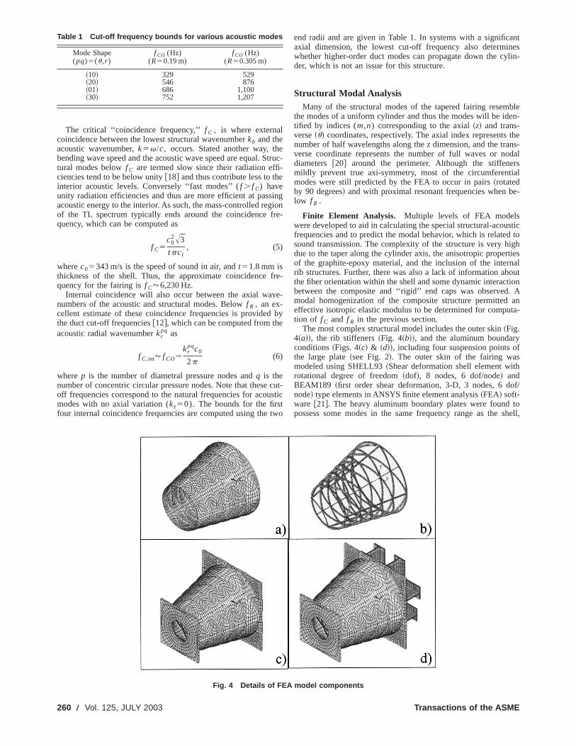
Finite Element Analysis. Multiple levels of FEA modelswere developed to aid in calculating the special structural-acousticfrequencies and to predict the modal behavior, which is related tosound transmission. The complexity of the structure is very highdue to the taper along the cylinder axis, the anisotropic propertiesof the graphite-epoxy material, and the inclusion of the internalrib structures. Further, there was also a lack of information aboutthe fiber orientation within the shell and some dynamic interactionbetween the composite and ‘‘rigid’’ end caps was observed. Amodal homogenization of the composite structure permitted aneffective isotropic elastic modulus to be determined for computa-tion of f C and f R in the previous section.

The most complex structural model includes the outer skin~Fig.4~a!!, the rib stiffeners~Fig. 4~b!!, and the aluminum boundaryconditions~Figs. 4~c! & ~d!!, including four suspension points ofthe large plate~see Fig. 2!. The outer skin of the fairing wasmodeled using SHELL93~Shear deformation shell element withrotational degree of freedom~dof!, 8 nodes, 6 dof/node! andBEAM189 ~first order shear deformation, 3-D, 3 nodes, 6 dof/node! type elements in ANSYS finite element analysis~FEA! soft-ware @21#. The heavy aluminum boundary plates were found topossess some modes in the same frequency range as the shell,

Table 1 Cut-off frequency bounds for various acoustic modes

Mode Shape(pq)5(u,r )

f CO (Hz)(R50.19 m)

f CO (Hz)(R50.305 m)

~10! 329 529~20! 546 876~01! 686 1,100~30! 752 1,207

Fig. 4 Details of FEA model components


which is why they were included in the model. Isotropic homoge-neous media was used to model the shell and rib composites, anda parametric study determined that an effective stiffness of 47 GPaproduces similar modal behavior to the real system. Dynamic be-havior from the model was evaluated by comparing the first eightnatural frequencies with those measured in the experiments. Thenovel beam-shell mixed FEA model proved to be computationallyeffective and accurate.

Figure 5 shows the first three mode shapes predicted by theFEA model. Only the shell is shown in Fig. 5 since the end capswould obstruct the cylinder modes. Both the end and side view ofthe lowest frequency mode~0,3! ~repeated! is shown at the toptwo panes of Fig. 5. The next two modes:~1,0! and ~0,2! areshown in the bottom two panes of Fig. 5. Similarity is notedbetween the predicted fairing modes and those for a uniform cyl-inder. Note that the lowest frequency bending mode for a cylin-drical shell does not correspond to the lowest indices: (m,n)5(0,1). It is interesting to observe that the low-frequency modesof the structure are predicted to respond globally as a shell, ratherthan a collection of smaller panels created by the rib stiffeners.This may or may not be true, since the unidirectional composite

stiffeners are actually stiffer than the isotropic model. A fewmodes occured in the end caps before the first structural mode at612 Hz, but did not cause appreciable normal displacement in theshell. The mode shapes and frequencies predicted by FEA aregiven in the first two columns of Table 2 below.

Experimental Tap Tests. Structural tap tests were conductedin order to experimentally determine the structural modal proper-ties. A PCB model 086C03 modally tuned hammer was used toexcite the structure while an array of 8 PCB 352B22 0.5-gramaccelerometers measured the response at various locations. Animaginary measurement grid consisting of 208 points~16 trans-verse angles~u! and 13 vertical planes~z!! was created. Threedifferent force input points atz5$0.31,0.38,0.46% m were used.Instead of measuring all 208 response points, representative arbi-trarily selected circumferences and vertical slices were measuredalong the fairing in order to try to corroborate the FEA results. Acurve-fit was performed on several of the frequency responsefunctions~FRFs! between various inputs and response locations inorder to extract global resonant frequency and damping character-istics to validate the FEA models. The complexity of the system

Fig. 5 First few structural mode shapes from FEA results

Table 2 Numerical and experimental structural modal properties.

Predicted ModeShape (m,n)5(z,u)

PredictedResonant Freq.

v r ,FEA ~Hz)

MeasuredResonant Freq.

v r ,Exp ~Hz)%Error Betweenv r ,FEA & v r ,Exp

MeasuredDamping

z ~%!

~0,3! 615 612 0.5 0.8~0,3! 618 627 21.2 0.7~1,0! 702 678 3.2 0.6~0,2! 761 699 8.1 0.8~0,4! 776 775 0.2 1.1~0,2! 818 787 3.8 1.0~0,4! 842 794 4.5 0.5


precluded fitting experimental data for mode shapes. Columns 3and 5 in Table 2 contain the resonant frequencies and damping~viscous model!, respectively, obtained from the curve-fit of theFRFs. Column 4 of this table shows the error between predictedand measured resonant frequencies. Errors range from 0.2–8.1%,which is considered good for a structure of this complexity. Thedamping values~0.8–1.1%! are perhaps higher than expected forthis type of material due to the existence of voids in the matrix.Figure 6 depicts a representative FRF and curve-fit taken at mea-surement point (z,u,r )5(39.5 cm, 56.25°, 24.4 cm) and drivepoint (z,u,r )5(18.9 cm, 56.25°, 24.4 cm). Some small resonantresponses are observed around 280, 400, and 470 Hz. The FEApredicted these modes to be corner flapping modes of the largeend cap and two weak accordion-like modes of the structure, re-spectively. It is the modes with large normal displacement whichcouple well to sound, and thus these modes were not of interestfor this study. Note from Table 2 that the lowest structural fre-quency is 612 Hz, meaning that the resonance-controlled region isexpected to end around 2361251,224 Hz. Thus, the mass con-trolled region is expected to extend from 1,224 Hz to the criticalfrequency off C56,230 Hz.

Acoustic Modal AnalysisSimilar to the fairing shell, the modes of the internal tapered

acoustic cavity conform well to those for a uniform cylindricalcavity with closed ends. These modes will also be referenced withrespect to the cylindrical coordinate system given by Fig. 3 andthe indices (o,p,q) or (opq). The first modal index,o, representsthe number of half wavelengths along thez-axis, the second,p,represents the number of nodal diameters occuring along thetransverseu coordinate, andq represents the number of radialnodes along ther direction in Fig. 3. The acoustic mode shapesare important for three reasons. First, the modal pressure distribu-tions could be examined for ‘‘problem modes,’’ when consideringthe payload location. More importantly, the predicted modeshapes can be used to estimate the cut off frequenciesf CO for thetruncated cone, which will be bounded by the predictions given inTable 1. Because internal coincidence occurs at these frequencies,worse transmission loss would be expected, which will be verifiedin measurements section. Also, the structural-acoustic couplinggiven by Eq.~2! indicates that the relative shape of thein-vacuostructural modes and rigid-wall acoustic modes will influence thenoise transmission. However, this relationship is of limited valuedue to the complexity of the coupling.

Finite Element Analysis. The rigid-wall acoustic cavitymodel of the fairing was created using a uniform tapered cylindri-cal boundary that neglected the internal ribs, since they wouldinsignificantly affect the acoustic modal properties of the system.FLUID30 elements~ANSYS 5.7! with properties for air at stan-dard conditions~density of 1.21 kg/m3, sound speed of 343 m/s,and static pressure of 100 kPa! were used to model the cavity.Mesh convergence was performed and the total resulting numberof elements and degrees of freedom were 1,244 and 4,976, respec-tively. The four degrees of freedom for each node were threeCartesian particle velocity components (Vx , Vy , andVz) and thepressure,P. A second FEA model included the speaker that wasused for the experimental modal analysis. It was modeled as arigid piston ~moving mass! on a spring-damper~spider! support.Since both acoustic FEA models yielded similar results, the sim-pler model without the speaker was adopted for the study. Thismodel is also consistent with the NRS measurements setup, whichdid not contain the attached speaker. Given the high degree ofideal nature in the model, the predicted acoustic modes are givena high degree of confidence, particularly at low frequency wheremodels are known to generally perform well. Figure 7 shows thefirst six predicted acoustic mode shapes. The axial-symmetricmode shapes are repeated~rotated by 90 deg!, but the repeats areomitted for brevity. The experimental modal analysis is presentedin the next section.

Experimental Results. The experimental acoustic modalanalysis was performed by exciting the fairing with the attachedspeaker atz5r 50 ~shown in bottom of Fig. 2!. A total of 260acoustic measurements were taken with the internal microphonespositioned at combinations of the following coordinates:r5$3.81,7.62,11.4,15.2% cm, u5$15,30,45,60,75,90,105,120,135,150,165,180% degrees, and across vertical planes atz5$10,20,30,40,50% cm. The FRF was computed between the inputto the speaker and each of the four array microphones and thusincluded the speaker dynamics, which are much lower frequencythan the first acoustic mode of the fairing cavity. Figure 8 shows atypical measured FRF between the speaker and an internal micro-phone located at (z,u,r )5(19.5 cm, 337.5 deg, 23 cm!. Notealso from the figure that the modes and speaker dynamics havebeen identified. The dominance by the fundamental~100! mode at301 Hz is typical of most all of the measured FRFs. However, theaxial zero modes~010!, ~020!, and~001! at 385, 613, and 788 Hz,respectively, will be shown in the next section to also be veryimportant for sound transmission. These three modes are used toestimate the internal coincidence frequencies, the bounds of which

Fig. 6 Representative FRF of structure


were given in the first three rows of Table 1. Interestingly, al-though they are significant for sound transmission, many of thesemodes appeared insignificant in the acoustic FRFs. The differenceresults from the direct excitation by the speaker for the FRF ver-sus excitation via transmission for the NRS measurement. Previ-ous studies focused mainly on the~100! mode as the primarycontributor to noise transmission@6,7#.

A curve-fit was performed on an arbitrary selection of 32 of the260 FRFs so that modal properties could be extracted. Naturalfrequencies and damping ratios for the first eight modes are givenin columns 3 and 5, respectively, of Table 3. The predicted modeshape and natural frequencies from the FEA analysis are given incolumns 1 and 2 of the same table, along with the error betweenpredicted and measured natural frequencies in column 4, which

are within 0.1–5.1% in magnitude. Repeated modes that havenearly identical natural frequencies are indicated~‘‘ 32’’ ! in col-umn 1 of Table 3.

Finally, note that when comparing the measured resonant fre-quencies of the structure and acoustic cavity in Tables 2 and 3, ingeneral the same modal frequencies do not show up in both tables,indicating that indeed the structural acoustic coupling is light.There are however, two frequencies in the vicinity of 612 and 787Hz that are given in the tables that appear for both the structureand the acoustic cavity. Although internal coincidence is also pre-dicted to occur for the acoustic modes at these two frequencies, itis not between the structural modes that have nearly identicalfrequency, since internal coincidence can only occur betweenmodes of the same transverse wavenumber,ku , which is related

Fig. 7 First few acoustic mode shapes from FEA results

Fig. 8 Representative FRF between speaker and cavity microphone


to modal indexn for the structure andp for the acoustic cavity.When comparing the modal indicesn andp from the first columnof Tables 2 and 3, one observes that (n53Þp52) at 612 Hz and(n52Þp51) at 787 Hz.

Measurement of Sound TransmissionNRS measurements are based upon a spatial average of mean-

square pressure measurements from the inside and outside of thestructure as given by Eq.~3!. To simulate a diffuse field, fourspeakers were arranged around the structure and driven with in-dependent white noise sources. Note that a previous work reportedthat directional effects in the radiation and reception patterns donot occur in finite cylinders@13#. A wide bandwidth~0–20 kHz!for the noise sources was desired due to the small scale of thestructure. The speakers and the structure were suspended 0.7 mabove the floor and the room volume was approximately 300 m3.An external microphone was traversed to 20 different measure-ment locations which were 1.5 cm from the surface of the shell.The 20 locations spanned across five different vertical heights:h5$10,20,30,40,50% cm, and four different transverse angles:u5$0,90,180,270% deg. An internal microphone boom was in-stalled 1.5 cm from the edge of the ribs. This microphone re-corded 20 internal measurements which were at the same heightand angles as the exterior microphone. Figure 9 depicts a top viewof the measurement setup. Signals were generated and measuredusing a Siglab MC20-84 dynamic signal analyzer. Bruel and Kjaer4190 microphones with B&K 2669 preamplifiers were used forthe acoustic measurements. Marchand PS-24 power amplifiersdrove the four KLH-9912 speakers to generate the external noisefield. Autospectrum measurements from the inside and outsidewere post processed and linearly averaged to determine the NRS.

A convergence study on the spatial sampling was performed bycomputing NRS using 1, 2, 4, 8, 16, and 20 sets of measurementpoints across the surfaces of the shell. The NRS was mostly con-verged by 8 points, and the difference between 16 and 20 pointswas indistinguishable. Thus, 20 was chosen as a suitable numberof points. Effects of angular and vertical position were also exam-ined. Little variation in NRS was noted between angles whenaveraging the 5 vertical measurement heights together. Variationwithin the vertical measurement planes was more pronounced,with the sharpest dips in NRS noted near the end caps, which isconsistent with modal pressure maxima and edge radiation effects.

Figure 10 shows the measured NRS for the structure using alinear frequency axis from 0–1000 Hz. Note that vertical dashedand dotted lines have been added at the frequencies of the acousticand structural resonances, respectively, which were obtained fromthe structural and acoustic modal analyses. In the low-frequencystiffness-dominated region of the NRS~100–250 Hz!, the reduc-tion is seen to range from 34–52 dB, with most frequencies above40 dB. The dip at very low frequency~40 Hz! is attributed to theHelmholtz frequency for the enclosure, which occurs due to leak-age. Two dips likely occured because an access door to the struc-ture had to be opened and closed 20 times to arrange the internalmicrophone at each measurement location, which may have cre-ated nonuniform leakage each time. Commensurate dips in theNRS are noted at most all of the acoustic resonant frequencies~e.g. 301 Hz (opq)5(100), 385 Hz~010!, 547 Hz~110!, 613 Hz~020!, 735 Hz ~210!, 788 Hz ~001!, and 840 Hz~120!. A Dip inthe NRS is not noted for the acoustic mode at 583 Hz. Most of thestructurally dominant resonances are seen not to influence theNRS, presumably due to the relatively high level of damping forthis composite structure. The exceptions are at 612, 787, 794, 845,

Table 3 Numerical and experimental acoustic modal properties.

Predicted ModeShape (opq)5(zur )

PredictedResonant Freq.

v r ,FEA ~Hz)

MeasuredResonant Freq.

v r ,Exp ~Hz)% Error Betweenv r ,FEA & v r ,Exp

MeasuredDamping

z ~%!

~100! 313 301 4.0 0.29~010!32 383 385 20.5 0.23~110!32 550 547 0.5 0.18~020!32 617 583 5.6 0.22'~020! 622 613 1.4 0.27~210!32 765 735 3.8 0.14~001! 787 788 20.1 0.20~120!32 815 840 23.1 0.33

Fig. 9 Noise transmission measurement setup


and 950 Hz. Each of these frequencies also coincides with anacoustic mode, so it is hard to decipher whether the acoustic,structural or both contribute to the NRS. There are three frequen-cies~612, 787–794, and 845 Hz! where the noise transmission isactually negative, indicating an amplification of the noise by thestructure. Modes at 612 and 787 Hz have already been associatedwith internal coincidence frequencies. The mode at 845 Hz isassumed to be associated with the 815 Hz~120! mode from theFEA, but is also near the~030! mode with a predicted naturalfrequency of 840 Hz. Note that since the accuracy of FEA modelsdeteriorate at higher frequency, the measured 840 Hz frequencymay actually be the~030! mode, which would have internal coin-

cidence as well. Again, as noted when examining Fig. 8, thesemodes do not have a particularly strong response in this FRF, buttransmit energy well due to coincidence. The~010! mode was alsoobserved to be a weak mode in most all of the acoustic FRFs, butis seen to have a significant dip in the NRS at that frequency~385Hz!, again attesting to the importance of internal coincidence forNRS. The 794 Hz dip appears to be due to the structural mode atthat frequency.

In Fig. 11, the NRS is replotted with a logarithmic frequencyaxis which extends from 100 to 20,000 Hz. The approximatestiffness-, resonance-, and coincidence-controlled regions of theNRS are indicated in the figure, as well as the probable contribu-

Fig. 10 Measured noise reduction spectrum showing acoustic and struc-tural modes

Fig. 11 Measured noise reduction spectrum „NRS… showing variousregions of transmission loss


tion by the ring frequency. Referring back to the section on trans-mission loss, the stiffness-controlled region will begin at 0 Hz andend at the first resonance, which is an acoustic cavity resonance at300 Hz. The ‘‘resonance-controlled’’ region was predicted to con-tinue through approximately twice the first structural resonancefrequency or~2361251,224 Hz!. Judging from the figure, thedips in NRS from the resonances are noted to stop around 1,500Hz and a general upward trend begins until a wide dip begins at6,000 Hz. The slope in the mass-controlled region is 28 dB perdecade rather than the classical 20 dB/decade mass law. Sincef Cwas predicted to be 6,230 Hz, this dip is attributed to externalcoincidence. The width of the dip is rather large~6,000–12,000Hz!, which may be attributed to effects of the stiffeners and/orring frequency effects@12#. Regardless, the dip is inconsequentialwhen compared to the levels at the singularities in the NRS thatoccur at internal coincidence frequencies and in the region aroundwhere the resonance- and mass- controlled regions meet.

Note that to improve the noise transmission behavior willlargely require the acoustically dominant modes and/or internalcoincidence phenomena to be controlled. Internal absorptive treat-ments are limited in rocket fairings due to the volume require-ments of the payload. The NRS could perhaps also be improved at612, 787, 794, 845, and 950 Hz by adding damping treatments orcontrol that targets these structural modes.

ConclusionsThe noise transmission behavior for a novel, advanced grid-

stiffened ~AGS! composite structure has been investigated. Thismaterial is being considered by the US Air Force for constructingexpendable space launch vehicles. A combined numerical/experimental approach was used to examine the physical mecha-nisms of noise transmission by the structure. Separate analyseswere performed on the structure and the acoustic cavity since thecoupling between the two was found to be very light. Finite ele-ment analysis permitted a smeared or average value for the com-posite elastic modulus to be determined, which in turn was used toestimate the ring and critical frequencies for the structure, sincethey influence transmission loss. Mode shapes were also predictedby FEA, which allow the modal pressure distributions to be ex-amined and which also permit investigation of the internal coin-cidence phenomena. Experimental modal analyses on the structureand cavity were also performed. Tap tests at various locationsaround the structure provided frequency response functions~FRFs! that were curve-fit to obtain resonant frequencies anddamping ratios. A speaker was used to drive the acoustic cavitywith a white input while the pressure response was measured in-side the cavity. Again, the measured FRFs were fitted to obtainresonant frequencies and damping ratios for the acoustic modes.Comparison of measured and predicted natural frequencies per-mitted corroboration of the FEA models. The resonances for thestructure and especially the acoustic cavity were found to signifi-cantly affect the noise transmission into the structure.

Finally, direct measurement of sound transmission was con-ducted based upon the noise reduction spectrum~NRS!, which iscomputed from the ratio of the spatial averages of acoustic pres-sures measured along the internal and external surfaces of theshell. Classic stiffness, resonance, and coincidence controlled re-gions were identified, which agreed very well with the predic-tions. The NRS was dominated by the sharp dips that were notedat most of the acoustic resonant frequencies. Internal coincidencewas found to play a significant role as well, since negative NRSvalues~amplification! was noted at these frequencies. The internalcut-off frequencies are good estimates of the internal coincidencefrequencies below the ring frequency. These frequencies were de-termined from the FEA results by identifying the axial-zero modes(kz50). External coincidence and possibly ring frequency effects

also impacted the sound transmission, as noted by the wide dip inthe NRS plot from 6–12 kHz. However, this dip is found to beinconsequential compared to the singularities found at some of theacoustic mode frequencies. Future transmission control will pro-vide a significant challenge due to the payload and weight require-ments for the launch vehicles. Since the NRS is dominated by theacoustic modes, control should focus on adding damping to theacoustic modes or focus on disrupting the internal coincidencephenomena. Once the effect of the acoustic modes is sufficientlyameliorated, additional marginal improvements could also be ex-pected by increasing the damping of certain structural modes.

AcknowledgmentsThe work was sponsored by the Air Force Research Laboratory

Space Vehicles Directorate~AFRL/VS!. The POC for this effort isDr. Steven A. Lane. The authors also acknowledge ANSYS, Inc.for the John Swanson Fellowship. Thanks also to David J. Be-lasco, Jr. for help with data collection and reduction.

References@1# Huybrechts, Steven, and Tsai, Stephen W., 1996, ‘‘Analysis and Behavior of

Grid Structures,’’ Comp. Sci. Technol.56~9!, pp. 1001–1015.@2# George, Tommy J., Herman Shen, M. H., Huybrechts, Steven M., Meink, Troy

E., and Wegner, Peter M., 2001, ‘‘Optimal Design of Composite ChambercoreStructures,’’ Compos. Struct.,52~3–4!, pp. 277–286, May–June.

@3# Griffin, Steven, Denoyer, Keith K., and Das, Alok, 1999, ‘‘Passive Vibroacous-tic Isolation for Payload Containers,’’ J. Intell. Mater. Syst. Struct.,10~0083-05!, pp. 83–87.

@4# Griffin, Steven, Hansen, Collin, and Cazzolato, Ben, 1999, ‘‘Feasibility ofFeedback Control of Transmitted Sound into a Launch Vehicle Fairing UsingStructural Sensing and Proof Mass Actuators,’’ AIAA99~1529!, pp. 2592–2602.

@5# Griffin, Steven, Hansen, Collin, and Cazzolato, Ben, 1999, ‘‘Feedback Controlof Structurally Radiated Sound into Enclosed Spaces Using Structural Sens-ing,’’ JASA, 106~5!, pp. 2621–2628.

@6# Griffin, Steven, Denoyer, Keith K., and Sciuli, Dino, 1998, ‘‘Hybrid Structural/Acoustic Control of a Sub-Scale Payload Fairing,’’SPIE Conference on SmartStructures and Integrated Systems, Vol. 3329 of 0277-786X, pp. 237–243.

@7# Griffin, Steven, and Denoyer, Keith K., 1998, ‘‘Experimental Sensor and Ac-tuator Location Procedure for Control of Dynamically Complex Smart Struc-tures,’’ SPIE Conference on Smart Structures and Integrated Systems, Vol.3329 of 0277-786X, pp. 717–723.

@8# Lane, Steven A., Kemp, J. D., Griffin, Steven, and Clark, R. L., 2001, ‘‘ActiveAcoustic Control of a Rocket Fairing Using Spatially Weighted TransducerArrays,’’ AIAA J., 38~1!, 112–119.

@9# Neple, Pascale, el Hafidi, Ali, and Lesueur, Claude, 2001, ‘‘On Sound Trans-mission Through a Truncated Isotropic Conical Shell: Experimental and Pre-liminary Numerical Results,’’Internoise 2001, The Hague, The Netherlands,August 27–30.

@10# Vipperman, Jeffrey S., Li, Deyu, Avdeev, Ilya, and Lane, Steven A., 2001,‘‘Characterization and Control of Sound Radiation in a Complex Fairing Struc-ture,’’ Internoise 2001, The Hague, The Netherlands, August 27–30.

@11# Denoyer, Keith K., Griffin, Steven, and Das, Alok, 1998, ‘‘Passive Vibroacous-tic Isolation for Reusable Launch Vehicle Payload Containers,’’AIAA/ASME/ASCE/AHS/ASC Structures, Structural Dynamics & Materials Conference,AIAA-98-1977, pp. 2248–2256, Longbeach, CA, April 20–23.

@12# Fahy, F., 1985,Sound and Structural Vibration, Academic Press, Inc., NewYork.

@13# White, Pritchard H., 1966, ‘‘Sound Transmission Through a Finite, ClosedCylindrical Shell,’’ JASA,50~5!, pp. 1124–1130.

@14# Manning, J. E., and Maidanik, G., 1964, ‘‘Radiation Properties of CylindricalShells,’’ JASA,36~9!, pp. 1691–1698.

@15# Cheng, L., 1994, ‘‘Fluid-structural Coupling of a Plate-ended CylindricalShell: Vibration and Internal Sound Field,’’ JSV,174, pp. 641–654.

@16# Koval, L. R., 1976, ‘‘On Sound Transmission into a Thin Cylindrical ShellUnder Flight Conditions,’’ JSV,48, pp. 265–275.

@17# Koval, L. R., 1978, ‘‘Effects of Cavity Resonances on Sound Transmissioninto a Thin Cylindrical Shell,’’ JSV,59, pp. 23–33.

@18# Blake, William K., 1986,Mechanics of Flow-Induced Sound and Vibration,Vol. 1, General Concepts and Elementary Sources, Academic Press, Inc., Lon-don.

@19# Blake, William K., 1986Mechanics of Flow-Induced Sound and Vibration,Vol. 2, Complex Flow-Structure Interactions. Academic Press, Inc., London.

@20# Blevins, Robert D., 1979,Formulas for Natural Frequency and Mode Shape,Van Nostrand Reinhold Co., New York.

@21# ANSYS, Inc., 2001, Canonsburg, PA 15317.


Jianhui Luo

Hae Chang Gea

Department of Mechanical and AerospaceEngineering,

Rutgers, The State University of New Jersey,Piscataway, NJ 08855

Optimal Stiffener Designfor Interior Sound ReductionUsing a Topology OptimizationBased ApproachA topology optimization based approach is proposed to study the optimal configuration ofstiffeners for the interior sound reduction. Since our design target is aimed at reducing thelow frequency noise, a coupled acoustic-structural conservative system without dampingeffect is considered. Modal analysis method is used to evaluate the interior sound level forthis coupled system. To formulate the topology optimization problem, a recently intro-duced Microstructure-based Design Domain Method (MDDM) is employed. Using theMDDM, the optimal stiffener configurations problem is treated as a material distributionproblem and sensitivity analysis of the coupled system is derived analytically. The norm ofacoustic excitation is used as the indicator of the interior sound level. The optimal stiff-ener design is obtained by solving this topology optimization problem using a sequentialconvex approximation method. Examples of acoustic box under single frequency excita-tion and a band of low frequency excitations are presented and discussed.@DOI: 10.1115/1.1569512#

1 IntroductionThe reduction of low frequency noise is of great interest in

designing transportation vehicles because the 20-200 Hz low fre-quency noise has an important influence on the product satisfac-tory quality. In the automobile passenger compartment, the lowfrequency noise can be generated by engine vibration or inducedby road roughness; in the aircraft cabin, the low frequency noisecan be originated from engines, propellers or aerodynamic forces.Although active vibration control is a fast growing research field,passive vibration controls from structural optimization techniquesare often used in practice due to their low implementation cost.Studies of noise reduction by structural modification are found inthe literature. Hagiwara et al.@1# investigated the reduction ofvehicle interior noise with shell thickness redistribution using thesensitivity information semi-analytically. Huff, Jr. and Bernhard@2# used a parametric shape optimization method in the reductionof the sound pressure level. Wodtke and Koopmann@3#, Constantsand Belegundu@4# introduced the structural modifications by plac-ing optimally sized point masses in order to minimize the radiatedsound power of vibrating structures.

In this paper, a topology optimization based approach is pro-posed to study the optimal configuration of stiffeners for interiorsound reduction. Since our design target is aimed at reducing thelow frequency noise, a coupled acoustic-structural conservativesystem without damping effect is considered. Modal analysismethod is used to evaluate the interior sound level for this coupledsystem @5#. To formulate the topology optimization problem arecently introduced Microstructure-based Design Domain Method~MDDM ! @6# is employed. Using the MDDM, the optimal stiff-ener configurations problem is treated as a material distributionproblem and sensitivity analysis of the coupled system is derivedanalytically. The optimal stiffener design is obtained by solvingthis topology optimization problem using a sequential convex ap-proximation method called Generalized Convex Approximation@7#.

The remainder of the paper is organized as follows: Section 2

introduces the modal analysis approach to calculating the fre-quency response for the coupled acoustic-structural system; Sec-tion 3 discusses the sensitivity analysis of frequency response forthis system. In Section 4, topology optimization problem is for-mulated and the solution procedure of identifying the optimal con-figurations of stiffeners for the reduction of the interior soundlevel is described. In Section 5, four numerical examples of anacoustic box under external excitations are presented. Conclusionremarks and future work are discussed in the final section.

2 Frequency Response of Coupled SystemsIn this section, frequency response of coupled acoustic-

structural systems is derived from the modal analysis method.Consider that a coupled acoustic-structural system consists of anenclosure surrounded by an elastic body and the elastic body issubjected to both force and displacement boundary conditions asshown in Fig. 1. Using the finite element method to discretize thecoupled system yields the following equations@8#

F Mss 0

Mas MaaG H ue

peJ 1FKss Ksa

0 KaaG H ue

peJ 5 H f s

0 J (1)

where the upper equation refers to the structural system and thelower equation refers to the acoustic system. In these equations,ue is the vector representing displacement components at the gridpoints of the structural finite element model,pe is the vector rep-resenting sound pressures at the grid points of the acoustic finiteelement model.f s represents the external forces applied to thestructure, such as mechanical excitations.Mss andKss are struc-tural mass and stiffness matrices,Maa andKaa are acoustic massand stiffness matrices.Mas and Ksa are acoustic-structural cou-pling matrices, and they have the property ofKsa52Mas

T . Thestructural and acoustic equations of motion are coupled throughthe matrix Mas which transforms the structural accelerations toacoustic excitations of the interior cavity, and through the matrixKsa which transforms the acoustic pressures to loads acting on thestructure.

If the external force has a harmonic form off seivt, then the

structural and acoustic responses can be expressed asueeivt and

Contributed by the Technical Committee on Vibration and Sound for publicationin the JOURNAL OF VIBRATION AND ACOUSTICS. Manuscript received June 1997;Revised October 2002. Associate Editor: R. L. Clark.


peeivt, wherev is the excitation frequency. Introducing these ex-

pressions to Eq.~1! yields the frequency response equation as

FKss2v2Mss Ksa

2v2Mas Kaa2v2MaaG H ue

peJ 5 H f s

0 J (2)

There are two different approaches to computing frequency re-sponse in Eq.~2!: the direct method and the modal analysismethod. The direct method is a rather straightforward approachthat solves Eq.~2! directly but it is very computationally expen-sive. On the other hand, the modal analysis method is extremelyattractive because both structural and acoustic modal density arerelatively low under the low excitation frequencies. Therefore, themodal analysis method is adopted in this study.

Since the mass and stiffness matrices are unsymmetric in thecoupled acoustic-structural system, the left eigenvectors are notthe same as the right ones. Using the modal analysis method, theright eigenvalue problem can be formulated as

FKss Ksa

0 KaaG H Cs

CaJ 5@L#F Mss 0

Mas MaaG H Cs

CaJ (3)

whereL is the eigenvalue matrix;Cs andCa are the right eigen-vector matrices corresponding to the structural and acoustic fieldsrespectively. Similarly, the left eigenvalue problem is representedas

$CsT Ca

T%FKss Ksa

0 KaaG5@L#$Cs

T CaT%F Mss 0

Mas MaaG (4)

where Cs and Ca denote the left eigenvector matrices of thestructural and acoustic fields. The M-orthonormal condition of thecoupled system is stated as follows:

$CsT Ca

T%F Mss 0

Mas MaaG H Cs

CaJ 5@ I # (5)

For large coupled acoustic-structural systems, it is impracticalto solve Eq.~3! and Eq.~4! directly because of the high compu-tational cost. Luo and Gea@5# proposed a symmetrization ap-proach to effectively extract eigenmodes with less computationaltime and storage. They also proved that the right eigenvectors andthe left eigenvectors of a coupled system can be related as

H Cs

CaJ 5 HLCs

CaJ (6)

Suppose that the forced frequency responses are expanded bythe right eigenvectors of the coupled system as

H ue

peJ 5Cj (7)

whereC5$Cs Ca%T denotes the right eigenvector matrix of the

coupled system,j is the coefficient matrix.Inserting Eq.~7! into the governing equations of Eq.~2! and

premultiplying both sides by left eigenvector matrixCT

5$CsT Ca

T%, the use of M-orthonormal condition leads to

~@L#2v2@ I # !j5CTH f s

0 J 5CsTf s (8)

DenoteCsT f s5p, the coefficient matrixj can be computed in the

following form

j i5pi

l i2v2 (9)

wherej i , pi and l i are thei th component ofj, p and L. Com-bining Eq.~9! with Eq. ~7!, the response of the coupled acoustic-structural system is recovered.

3 Sensitivity Analysis of Coupled SystemsWhen an optimization problem is solved by mathematical pro-

gramming algorithms, we must determine the effect resulting froma small perturbation in the current design on the objective andconstraint functions. This is known as the sensitivity analysis. Inthis study, frequency response sensitivities are the derivatives ofstructural response and the sound pressure with respect to thestructural modification design variables. With the correct fre-quency response sensitivity information, one can use various op-timization methods to arrive at a modified structure with reducedinterior sound level. The frequency response sensitivity,$ue8 ,pe8%

T, can be derived by differentiating Eq.~2! as

FKss2v2Mss Ksa

2v2Mas Kaa2v2MaaG H ue8

pe8J 52FKss8 2v2Mss8 0

0 0G H uc

peJ

(10)

whereKss8 and Mss8 are the derivatives of the structural stiffnessand mass matrices with respect to the design variable, respec-tively.

If we define a pseudo loadgs52@Kss8 2v2Mss8 #ue , Eq. ~10!can be rewritten as

FKss2v2Mss Ksa

2v2Mas Kaa2v2MaaG H ue8

pe8J 5 Hgs

0 J (11)

Eq. ~11! has the same form as the frequency response governingequations in Eq.~2! except the excitation force has been changedfrom f s to gs . Therefore, the solution of Eq.~11! can be obtainedin the same way as shown in the previous section.

Assume response sensitivities can be decomposed as,$ue8 ,pe8%

T5Ch with h being the undetermined coefficient matrix.Put this expansion into Eq.~11! and premultiply both sides byCT, we have

~@L#2v2@ I # !h5CTHgs

0 J 5CsTgs (12)

DenoteCsTgs5q, then coefficient matrix can be determined in the

indices form

h i5qi

l i2v2 (13)

With Eq. ~13!, the frequency response sensitivity,$uc8 ,pe8%, can becalculated easily.

4 Solution ProceduresIn this section, the solution procedures of identifying the opti-

mal configuration of stiffeners placement for the reduction of theinterior sound level are discussed.

Fig. 1 A coupled acoustic-structural system


The overall interior sound level for the acoustic field is evalu-ated as

SPL51

m (i 51

m

~10 log10@pi /p0#2! (14)

wherepi denotes the sound pressure at thei th node,m is the totalnumber of nodal points in the acoustic field,p0 is a referencepressure, normally, chosen as 231025 Pa.

Although SPL is a direct indicator of sound noise, it inheritsstrong localized effects from individual nodal pressure. Therefore,if this function is used as the objective function in the optimiza-tion process, search algorithm will exhibit unstable oscillationsand consequently have difficulty to converge. Consider the factthat the level of interior sound is fully determined by the acousticexcitation, that can be measured by the magnitude of2v2Masuefrom Eq.~2! for a given excitation frequency. The minimization ofthe norm of2v2Masue can lead to the reduction of SPL. There-fore, the minimization of the acoustic excitation is chosen as theobjective function. In our numerical examples, iteration historiesof SPL are also listed for the purpose of comparing the soundpressure level reductions from the optimization process.

When a structure is subjected to a band of frequency excitations@v0 ,v1#, the objective function can be modified as

Minimize1

v12v0E

v0

v1

i2v2Masue~v!idv (15)

And, the overall interior sound level from Eq.~14! can be definedas

SPL51

v12v0E

v0

v1S 1

m (i 51

m

~10 log10@pi~v!/p0#2!D dv

(16)

Recently, the stiffener layout optimization problem is tackledby material distribution formulations, in which a given amount of‘‘artificial’’ stiffener material is dispersed optimally to the basestructure for the best structure performance. The material modelfor the combination of base material and ‘‘artificial’’ stiffener ma-terial is often borrowed from various theories of composite mate-rials. This method is called the topology optimization because thetopology of stiffener design is to be optimized. Diaz and Kikuchi@9# used this technique on solving stiffener layout design optimi-zation under natural frequency and they applied the homogeniza-tion theory@10# to evaluate the material properties of the compos-ite consisting of the base and stiffener material. In this paper, aMicrostructure-based Design Domain Method~MDDM ! intro-duced by Gea@6# is applied to model the add-on stiffener. In theMDDM, material is treated as a ‘‘composite’’ consisting of matrixand spherical inclusion materials. The effective material propertiesof the i th element is expressed in the form

k~ i !5k0S 11c1

~ i !~k12k0!

~12c1~ i !!a0~k12k0!1k0

D (17)

m~ i !5m0S 11c1

~ i !~m12m0!

~12c1~ i !!b0~m12m0!1m0

D (18)

with

a051

3

11n0

12n0(19)

b052

15

425n0

12n0(20)

where subscripts 0 and 1 represent matrix and inclusion materials;k and m denote the bulk modulus and the shear modulus.n0 isPoisson’s ratio of the matrix, andc1

( i ) is the volume fraction of theinclusion material in thei th element. Using this model, the vol-

ume fraction,c1( i ) , is treated as the design variables in the stiffener

topology optimization formulation: asc1( i )50 no stiffener is re-

quired andc1( i )51 stiffener exists. Using these relation,Kss8 and

Mss8 under the pseudo load can be directly calculated.Generally, the total allowable weight of the structure is consid-

ered as a design constraint that cannot exceed a prescribedamount. The optimization problem of minimizing acoustic excita-tion is stated as,

Minimize i2v2Masuei (21)

Subject To: (i 51

N

rv i~11c1~ i !!<W (22)

where r denotes the material density,v i is the volume ofi thelement,c1

i is the design variable as described previously,N is thenumber of elements, andW is the upper limit of total weight.

In order to search for the optimal stiffener topology, the numberof design variables is related to the number of finite elements usedin the structural model. Therefore, the optimizer used here mustbe very efficient in handling a large number of design variables. Inthis paper, the Generalized Convex Approximation~GCA! methodintroduced by Chickermane and Gea@7# is used to formulate andsolve the topology optimization problem. In the GCA, functionsare approximated as the sum of a series of separable functions ofthe design variables as

f ~x!> f ~xk!2(i

n

bi~xik2di !

r i1(i

n

bi~xi2di !r i (23)

wherebi , di and r i are a set of approximation parameters to bedetermined, andf (xk) is the value of the original function at thekth design. Function values and first order sensitivity informationfrom the current and previous design is utilized to determine thevalues of the approximation parameters. The approximation prob-lem is solved iteratively using mathematical programming to gen-erate the next design. This process continues until a satisfactorydesign is reached.

5 Numerical ExamplesOptimal stiffener designs of an aluminum alloy~1100-H14! box

using the proposed topology optimization based method are pre-sented in this section. The aluminum box of 30 cm340 cm350 cm is fixed at four bottom corners and under various externalexcitations. The aluminum plate has thickness 0.2 cm, Poisson’sratio 0.33, Young’s modulus 6.931010 Pa, density 2.73103 kg/m3 and the box without any stiffeners weights 5.076 Kg.The ‘‘artificial’’ stiffen material has the same density as the basematerial but with 100 times higher strength in order to simulatethe strong rigidity effect produced by stiffeners. The upper weightlimit of the add-on ‘‘artificial’’ stiffen material is set to be 10% ofthe total base weight. That gives the total allowable weight of thewhole structure be 5.5836 Kg. In the initial design, the add-on‘‘artificial’’ stiffen material is uniformly distributed to the box inorder to produce an unbiased starting point. From the analyses ofthe initial design, we found 20 structural eigenmodes and 3 acous-tic eigenmodes including one Helmholtz mode for the uncoupledsystem in the range of 0 to 500 Hz. Then, a coupled acoustic-structural analysis was performed. We found that the eigenfre-quencies of the uncoupled systems were shifted only slightly afterbeing coupled in the same frequency range. In Table 1, eigenfre-quencies in the range of 0 to 500 Hz for uncoupled and coupledsystems are listed for comparison.

Since we are only interested in the low frequency sound reduc-tion, damping effect for the coupled acoustic-structural systemwas neglected. In the structural field, 1536 4-node plate elementsare used and each of them is also treated as design variable for thestiffener design optimization formulation. In the acoustic field,4096 8-node solid elements are constructed. To reduce the interior


sound level, the norm of acoustic excitation is chosen as designobjective as we previously discussed. Four optimal design ex-amples under different external excitations are presented below.

5.1 Case 1. In the first case, a unit harmonic excitation withfrequency ofv550 Hz is applied at the center of the top plate asshown in Fig. 2. Using the proposed methodology, the norm ofacoustic excitation is reduced from 8.609643e-7 to 4.758937e-7 inten iterations and the overall interior sound decreased from 91.89dB to 68.97 dB. The iteration history is showed in Fig. 3 and thetrend of SPL reduction is listed in Table 2. The final stiffenerconfigurations is shown in Fig. 4. It was found that the stiffener ismainly concentrated in the region where the external force ap-plies, which is reasonable because the excitation frequency islower than resonance frequencies of the system. The uncoupledstructural frequencies and the coupled system frequencies in therange of 0 to 200 Hz are listed in Table 3. Comparing to the initialdesign with uniformly distributed stiffener material, we found thatthe final design also exhibits great changes of natural frequenciesand mode shapes.

5.2 Case 2. In the second case, the unit harmonic excitationwith the same excitation frequency as in the case 1 is applied tothe center point of the flank plate as shown in Fig. 5.

Iteration history of the objective function is shown in Fig. 6 andwe found the acoustic excitation is decreased from 6.246733e-7 to9.847646e-8 with the overall interior sound level reduction from76.73 dB to 51.92 dB in ten iterations. The result of the optimalstiffeners placement is shown in Fig. 7 and we can see the stiff-

Fig. 2 A box under an excitation loading at the center of thetop plate

Fig. 3 Iteration history of the objective function in case 1

Fig. 4 Optimal configuration of the stiffeners placement incase 1

Table 1 Coupled and uncoupled eigenfrequencies of a 30 cmÃ40 cmÃ50 cm aluminum box

Modenumber

Structuralfrequency

~Hz!

Acousticfrequency

~Hz!

Coupledfrequency

~Hz!

1 - 0.00 0.002 114.95 - 117.023 130.72 - 129.924 179.50 - 178.675 195.32 - 194.996 195.36 - 196.097 231.06 - 239.078 242.49 - 241.669 257.62 - 254.44

10 291.94 - 291.3511 302.71 - 302.7112 323.13 - 304.2113 335.41 - 330.4014 - 344.05 370.6115 387.39 - 382.7016 389.28 - 386.7517 411.79 - 411.7218 418.62 - 418.6219 - 430.06 443.0220 443.03 - 443.3321 462.87 - 452.7322 484.05 - 482.9423 494.91 - 495.40

Table 2 Trend of interior SPL reduction in case 1

Iterationnumber

Sound Pressure Level~dB!

Weight~Kg!

initial 91.89 5.58361 89.62 5.58362 80.87 5.58363 77.05 5.58364 75.64 5.58365 74.33 5.58366 72.08 5.58367 70.88 5.58368 70.52 5.58369 70.26 5.5836

10 68.97 5.5836


eners are also mostly located in the external force applied region.Table 4 shows the trend of interior SPL reduction throughout theiterations. The corresponding uncoupled structural frequenciesand coupled system frequencies in the range of 0 and 200 Hz arelisted in Table 5. The final design also experiences changes innatural frequencies and mode shapes from the initial design.

5.3 Case 3. In the third case, a unit harmonic excitationwith higher frequency is applied at the center of the top plate. Theexcitation frequency is chosen asv5150 Hz. We found the ob-jective function reduced from 2.811064e-5 to 1.548597e-5 and theoverall interior sound decreased from 80.13 dB to 67.03 dB afterten iterations. The iteration history is showed in Fig. 8 and thetrend of SPL reduction is showed in Table 6. Fig. 9 shows the

optimal stiffener location. Unlike the first two cases, in this casethe locations of stiffeners are spread out to different region of thebox. This is due to the fact the excitation frequency is in themiddle of several resonance frequencies of the system. To mini-mize the acoustic excitation, the add-on stiffeners try to reduce theeffects from all these resonance modes as much as possible. Thenatural frequencies below 200 Hz of the final design are alsolisted in Table 7 for reference.

5.4 Case 4. In the last example, the stiffener design under aband of frequency excitation is studied. A unit harmonic excitationis applied at the center of the top plate with a band of low exci-tation frequencies ranged from 20 to 100 Hz. A modified objectivefunction, Eq. ~15!, is used here. Since the excitation frequencyrange falls below any resonance frequency, the optimal stiffenerlocation turns out to be very similar to that of the first case as Fig.4. We found the objective function is reduced from 3.106249e-7 to1.842361e-7 and the overall interior sound defined in Eq.~16! isdecreased from 93.53 dB to 75.16 dB after ten iterations. Fig. 10shows the interior SPL comparison between the initial design andthe final design within the exciting frequency range.

Fig. 5 A box under an excitation loading at the center of theflank plate



Table 3 Natural frequencies of the final design in case 1

Modenumber

Structural frequency~Hz!

Coupled frequency~Hz!

1 - 0.002 70.18 72.313 120.74 120.274 120.87 120.535 124.97 125.106 138.17 146.127 147.54 148.258 177.84 177.519 185.15 184.02

10 190.37 187.38

Table 4 Trend of SPL reduction in case 2

Iterationnumber


Weight~Kg!

initial 76.73 5.58361 72.20 5.58362 61.03 5.58363 58.29 5.58364 57.33 5.58365 56.62 5.58366 56.90 5.58367 55.69 5.58368 53.92 5.58369 52.12 5.5836

10 51.92 5.5836


Modenumber



1 - 0.002 104.94 107.273 117.86 117.134 158.14 157.365 167.27 167.436 188.17 195.37


6 Conclusion and Future WorkIn this paper, optimal stiffener design for interior sound reduc-

tion of coupled acoustic-structural system is studied. Forced fre-quency response and its sensitivity of this coupled system weresolved by the modal analysis method. Using a topology optimiza-tion based approach, the optimal stiffener placement problem wasconverted into an optimal material distribution problem. Insteadof using the overall interior sound level directly, the norm ofacoustic excitation was used as the objective function and fromour numerical examples, it showed the acoustic excitation is agood indicator for sound reduction. At low frequency excitations,the optimal stiffeners might be applied to the region near theexternal force source, however when the excitation frequency isamong several resonance frequencies, stiffener might be placedthroughout the structure in order to compensate the resonancemodes involved. In this work, a conservative system with nodamping effect is considered, therefore the proposed approach isonly valid for single frequency excitation or a band of lowfrequency excitations without any resonance frequency included.More general method to handle damping is currently underinvestigation.

References@1# Hagiwara, W., Kozukue, W., and Ma, Z. D., 1993, ‘‘The Development of

Eigenmode Sensitivity Analysis Methods for Coupled Acoustic-Structural Sys-tems and Their Application to Reduction of Vehicle Interior Noise,’’ FiniteElem. Anal. Design,14, pp. 235–248.

@2# Huff, J. E., Jr., and Bernhard, R. J., 1995, ‘‘Acoustic Shape OptimizationUsing Parametric Finite Elements,’’ASME 1995 Design Engineering Techni-cal Conferences, DE-Vol. 84-2, pp. 577–584.

@3# Wodtke, H. W., and Koopmann, G. H., 1995, ‘‘Quieting Plate Modes withOptimally sized Point Masses—A Volume Velocity Approach,’’ASME 1995Design Engineering Technical Conferences, DE-Vol. 84-2, pp. 647–654.

@4# Constans, E., and Belegundu, A., 1996, ‘‘Minimizing Radiated Sound Powerfrom Vibrating Shells,’’The 6th AIAA/NASA/ISSMO Symposium on Multidis-ciplinary Analysis and Optimization, Bellevue, WA, Paper 96-4111, pp. 1106–1116.

@5# Luo, J. H., and Gea, H. C., 1997, ‘‘Modal Sensitivity Analysis of CoupledAcoustic-Structural Systems,’’ J. Sound Vib.,119, pp. 545–550.

@6# Gea, H., 1996, ‘‘Topology Optimization: A New Micro-Structure Based De-sign Domain Method,’’ Comput. Struct.,61„5…, pp. 781–788.



Fig. 10 Interior SPL comparison between the initial designand the final design

Table 6 Trend of interior SPL reduction in case 3

Iterationnumber


Weight~Kg!

initial 80.13 5.58361 79.59 5.58362 77.39 5.58363 74.91 5.58364 75.88 5.58365 73.40 5.58366 71.20 5.58367 70.46 5.58368 68.99 5.58369 67.63 5.583610 67.03 5.5836


Modenumber



1 - 0.002 88.77 90.393 115.09 115.624 161.26 160.885 166.55 166.006 173.40 173.79


@7# Chickermane, H., and Gea, H. C., 1996, ‘‘A New Local Function Approxima-tion Method for Structural Optimization Problems,’’ Int. J. Numer. MethodsEng.,39, pp. 829–846.

@8# Craggs, A., 1971, ‘‘The Transient Response of a Coupled Plate-Acoustic Sys-tem Using Plate and Acoustic Finite Elements,’’ J. Sound Vib.,15, pp. 509–528.

@9# Diaz, A. R., and Kikuchi, N., 1992, ‘‘Solutions to Shape and Topology Eigen-value Optimization Problems Using a Homogenization Method,’’ Int. J. Nu-mer. Methods Eng.,35, pp. 1487–1502.

@10# Bendsøe, M. P., and Kikuchi, N., 1988, ‘‘Generating Optimal Topologies inStructural Design Using A Homogenization Method,’’ Comput. Methods Appl.Mech. Eng.,71, pp. 197–224.


Yuji OhueAssociate Professor,

Department of Intelligent MechanicalSystems Engineering,

Kagawa University,Hayashi, Takamatsu, 761-0396, Japan


Akira YoshidaProfessor

Mem. ASME,Department of Mechanical Engineering,

Okayaya University,Tsushima-naka, Okayama, 700-8530, Japan


New Evaluation Method on GearDynamics Using Continuous andDiscrete Wavelet TransformsThe aim of this study is to propose a new evaluation method of gear dynamics using thecontinuous and discrete wavelet transforms. The wavelet transform (WT) is a method forthe time-frequency analysis of signals. In order to evaluate the difference in the geardynamics due to the gear materials, which are sintered and steel ones, the dynamiccharacteristics of gears were measured using a power circulating gear testing machine.The gear dynamics were analyzed in a time-frequency domain by the continuous anddiscrete WTs. The new evaluation method using the WTs proposed in this paper was moreuseful compared with the conventional one to investigate the damping characteristic andthe dynamic condition of the gear equipment.@DOI: 10.1115/1.1547465#

Introduction

Generally, the dynamic signals in the field of engineering prob-lems such as vibration, sound and so on, have been analyzed usingthe fast Fourier transform~FFT!. The FFT has been the mostcommon method to analyze the frequency properties of the sig-nals. In the FFT analysis, the signal as the function of time isconverted to the power spectra in a frequency domain. However,except for a special case, the frequency components of the mostsignals encountered in the engineering problem change with time.Based on the FFT alone, it is hard to investigate whether thefrequency components of the signals vary with time or not, eventhough the phase of the Fourier transform relates to time shifting.The FFT analysis is no more adequate for those applications.Therefore, it is significant and important to adopt the time-frequency analysis for those signals varying with time@1–3#.

It is possible by using the time-frequency analysis to investigatehow the frequency components of the signal vary with time. Thetime-frequency analysis can provide more beneficial informationabout the frequency compared with the FFT. During the last twodecades, a new mathematical technique for the time-frequencyanalysis, which has been called the wavelet transform~WT!,has been extensively developed@1,2#. The WT has some fea-tures different from those of the short-time fast Fourier trans-form or the Wigner-Ville distribution. Applications of the WTare actively studied in a variety of the fields of engineeringscience@4–7#.

Gears have been employed in automobiles, motorcycles, indus-trial robots and so on. The gears are an important machine ele-ment to transmit the power and to change the speed of the equip-ment. The FFT is generally used for analyzing the gear dynamics.However, it is important to evaluate the gear dynamic perfor-mance more precisely using WT. Therefore, in order to evaluatethe difference in the gear dynamics due to the gear materials, thedynamic performances of sintered and steel gears were measuredat gear rotational speeds of 1600 rpm to 10,000 rpm, using apower circulating gear testing machine. The gear dynamics con-cerned with tooth root strain, vibration acceleration of gear boxand sound near gear box, were analyzed in the time-frequencydomain by the continuous WT, and the signals of the gear dynam-ics were decomposed and reconstructed by the discrete WT. Thevalidity of the new evaluation method by the WT is discussed.

Test Gear and Testing MachineTable 1 and Fig. 1 show the specification and the shapes of gear

pair, respectively. The module and the pressure angle of the gearpair are 5 mm and 20 deg., respectively. The contact ratio of thegear pair is 1.246. The gear has 16 teeth and a face width of 6mm. The materials of the test gears are sintered and steel~JIS;SCM440! ones. Those test gears were induction-hardened beforegrinding of tooth surface. The material of the mating pinion issteel ~JIS: SCM415!. The chemical composition of the sinteredmaterial is almost the same as that of the steel SCM440. Manypores existed in the sintered great. Generally, the sintered materi-als have higher damping ratio due to the pores, compared with thesteel ones. The density of the sintered gear in this study is 6.8g/cm3. The Young’s modulus and Poisson’s ratio of the sinteredgear are 152 GPa and 0.25, and those of the steel gear are 206

Contributed by the Technical Committee on Vibration and Sound for publicationin the JOURNAL OF VIBRATION AND ACOUSTICS. Manuscript received May 2002;Revised Sept. 2002. Associate Editor: R. P. S. Han. Fig. 1 Shapes and dimensions of gear pair

Table 1 Specification of gear pair

Pinion GearModule mm 5Pressure angle deg. 20Number of teeth 15 16Addendum modification 0.571 0.560coefficientTip circle diameter mm 90.71 94.60Center distance mm 82.55Face width mm 18 6Contact ratio 1.246Accuracy* Class 1 Class 1Tooth surface finishing Grinding

*JIS B 1702


GPa and 0.3, respectively. Figure 2 shows the tooth profile errorsof test gear pairs. The tooth surfaces of both gears and pinion werefinally ground. The tooth profile errors of both sintered and steelgears and almost the same. The accuracy of the test gear pairs arein class 1 according to Japanese industrial standard~JIS B 1702!.

The test apparatus shown in Fig. 3 is a power circulating typegear testing machine with a center distance of 82.55 mm. The testgear was driven at an interval of 200 rpm within a range of rota-tional speedsn2 of 1600 rpm to 10,000 rpm. The loading torquewas statically applied to the gear shaft by a lever loading withdead weights and a torsional coupling. The torsional torque wastaken as a scale for loading. In this experiment, the value of thetorque was 30 Nm, which corresponds to a load per unit facewidth of 142 N/mm in the normal direction to the tooth surface.The gear pair was lubricated with a gear oil by pressure feeding ata flow rate of 750 ml/min and an oil temperature of 313 K.

The dynamic tooth root strain was measured using a dynamicstrain amplifier and a wire strain gage with a gage length of 0.3mm, which was bonded on a compression side of the root fillet ofthe gear. The vibration acceleration of the gear box was detectedby a piezo-electric pickup through an amplifier. The pickup has amaximum response frequency of 20 kHz. The sound pressure nearthe gear box was detected by a condenser type microphone havinga maximum response frequency of 12.5 kHz. The microphone waslocated at a distance of 300 mm from the side of the gear box.These signals were stored into a data recorder with a synchronoussignal obtained by a phototransistor and two disks with slits whichwere fixed on both shifts of the gear and the pinion. These storedsignals were analyzed using a computer with an A/D converterboard.

Wavelet Transform

Continuous Wavelet Transform. The continuous wavelettransform~CWT! of a function f (t) is defined as follows.

~Wc f !~b,a!5uau21/2E2`

`

f ~ t !cS t2b

a Ddt (1)

Where, thec(t) indicates the conjugate of a mother wavelet func-tion c(t). The a andb indicate the parameters on frequency andtime. The Gabor function defined by Eq.~2! was adopted as themother wavelet functionc(t) in this study

c~ t !5p21/4S vp

g D 1/2

expH 21

2 S vp

g D 2

1 ivptJ (2)

Where,vp is a center of angular frequency, andg is a constantand was set to bep(2/ln 2)1/255.336. Figure 4 shows an exampleof the Gabor function and its Fourier spectrum. The integral forEq. ~1! was calculated using the trapezoidal rule and the calcula-tion results are expressed using the following equation.

u~Wc f !u5A$Re~Wc f ~%21$Im~Wc f ~%2 (3)

Where, Re(Wc f ) and Im(Wc f ) are the real and the imaginaryparts in Eq.~1!. To express the wavelet map, that is the intensitymap in a time frequency domain, the intensity calculated by theCWT was normalized by the maximum intensity in the map.

Discrete Wavelet Transform. When the coordinates~b, a! ofthe CWT shown in Eq.~1! are discretized to the coordinates(22 j k,22 j ) using two integersj andk, the discrete wavelet trans-form ~DWT! is defined as follows.

dk~ j !52 j /2E

2`

`

f ~ t !c~2 j t2k!dt (4)

Where,dk( j ) is equal to (Wc f )(22 j k, 22 j )). j is calledlevel. The

inverse discrete wavelet transform~IDWT! is defined as

f ~ t !'(j

gj~ t ! (5)

The functiongj (t) on the wavelet component is given by

Fig. 2 Tooth profile errors of gear pair

Fig. 3 Power circulating gear testing machine and measurement system of dynamic performance ofgear pair


gj~ t !5(k

dk~ j !c~2 j t2k! (6)

Suppose thatf j (t) is the function at a levelj, f i(t) is satisfied withthe following relation.

f j~ t !5(k

ck~ j !f~2 j t2k! (7)

Where, $ck( j )% is a sequence at a levelj, and f(t) is a scaling

function. The scaling functionf(t) and the mother wavelet func-tion c(t) are satisfied with the two-scale relations as follows.

f~ t !5(k

pkf~2t2k! (8)

c~ t !5(k

qkf~2t2k! (9)

Where,$pk% and$qk% are two-scale sequences. The algorithms ofthe decomposition and the reconstruction using the DWT and theIDWT on the functionf (t) are given as Eqs.~10! and ~11!.

ck~ j 21!5(

la122kcl

~ j !

dk~ j 21!5(

lb122kcl

~ j !6 (10)

ck~ j !5(

l@pk22lcl

~ j 21!1qk22ldl~ j 21!# (11)

Where,$ak% and $bk% are the sequences to decompose the func-tion f j (t) at a levelj. Therefore, the decomposition and the recon-struction on the functionf (t) are concluded into the calculationsusing the sequences$ak%, $bk%, $pk% and $qk%. The functionsgj (t) and f j (t) at a levelj are able to be found by using Eqs.~6!and~7!. The functionf j (t) decomposed into the functiongj (t) onthe wavelet component is satisfied with the following relation.

f ~ j !~ t !5 f j 21~ t !1gj 21

~ t !5gj 21~ t !1gj 22~ t !1gj 23~ t !1•••

(12)

In this study, the scaling and the mother wavelet functionsbased on the cardinal B-spline function in order ofm54 wasadopted. The cardinal B-spline functionNm(t) in order of m isdefined as follows@1#.

Nm~ t !51

~m21!! (k50

m

~21!kS m

kD ~ t2k!1

m21 (13)

Figure 5 shows the scaling functionf(t) and the mother waveletfunction c(t) based on the functionN4(t), that is the cardinalB-spline function in order of 4. The functionf(t) is equal to thefunctionN4(t). From this figure, it is understood that the functionc(t) is very smooth and is very similar to sinusoidal functions.The sequences$ak%, $bk%, $pk% and $qk% are given in the refer-ence@1#.

Conventional Evaluation of Gear DynamicsFigure 6 shows the examples of the dynamic and static tooth

root strains or stresses measured in this experiment. Generally,in order to evaluate the dynamic load of the gear pair, the dyna-mic load ratio sdmax/ssmax, that is the ratio of the maximumdynamic tooth root stresssdmax to the maximum static tooth

Fig. 4 Gabor function

Fig. 5 Scaling and wavelet functions based on cardinalB-spline In order of mÄ4

Fig. 6 Dynamic and static tooth stresses


root stressssmax, has been used. In this study, the tooth rootstress at a rotational speedn2 of 6.6 rpm was adopted as the staticstressssmax.

Figure 7 shows the dynamic load ratiosdmax/ssmax plottedagainst the rotational speedn2 of gear. The frequencyf z indicatesthe tooth mesh frequency. The natural frequency of the gear pairincluding the shafts, which support the gear pair, was calculatedusing a program given in reference@8#. The equation of motionfor the calculation of the natural frequency of the gear pair isgiven by

Mx1Dx1K~ t,x!x5W1(i

2

Ki~ t,x!ei~ t ! (14)

where,M is the equivalent inertia mass of gear pair along the lineof action,D is the damping coefficient between gear pair includ-ing the shafts,K is the stiffness of gear pair,W is the static load,ei is the tooth profile error andx is the relative displacement alongthe line of action. Subscripti indicates the pinion (i 51) and thegear (i 52). Then, the natural frequencyf e is calculated using thefollowing equation.

f e51

2pA 1

TzE

0

TzK~ t,x!

Mdt (15)

Where,Tz is the tooth mesh period. In this experiment, the calcu-lated value off e was approximately 2.56 kHz. The gear box washit by a hammer to measure its natural frequency in the horizontaldirection of the gear box using the FFT. As the result, the naturalfrequency of the gear box was about 5.0 kHz. From Fig. 7, forboth the sintered and steel gears, the ratiosdmax/ssmax increaseswith fluctuation asn2 increases. The ratiosdmax/ssmax has threepeak values atn254200 rpm (f z51.12 kHz!, 6000 rpm (f z51.60 kHz! and 9000 rpm (f z52.40 kHz!, since the tooth meshfrequency and its harmonics coincide with both the natural fre-quencies of the gear pair and the gear box. Namely, the gear pairfor both the sintered and steel gears became the resonance condi-tions at their speeds. The ratiosdmax/ssmaxof the sintered gear ismostly smaller than that of the steel one againstn2 . Therefore, itis obvious that the sintered gear is superior to the steel one fromthe viewpoint of the damping characteristics.

Analysis of Gear Dynamics Using WTIn the previous section, the conventional evaluation method

was employed for evaluating the gear dynamic load. The conven-tional evaluation method, however, has not taken into account theinformation on the time and the frequency contained in the gear

dynamic load and used only the maximum value of the gear dy-namic load. Thus, the information of the gear dynamic load in thetime-frequency domain is important to evaluate the great perfor-mance in detail. In this section, the dynamic tooth root strains areanalyzed in the time-frequency domain using the WT.

Figure 8 shows the waveform of the tooth root strain~top of thefigure!, its WT map ~lower left of the figure! and the analyzedresult using the FFT~lower right of the figure! at a rotationalspeedn2 of 1800 rpm. The WT maps of both the gears wereobtained using the CWT. The WT map shows the intensity of thetooth root strain in the time-frequency domain. In the WT map,not only the frequency components but also the change of theintensity of each frequency in the tooth root strain with the timecan be provided more precisely, compared with the FFT analysis.In the WT maps of the sintered and steel gears, each intensity intwo regions above and belowf z5480 Hz indicates each peak. Thecontact time of one tooth pair atn251800 rpm is approximately2.6 ms. Suppose that the wave of the tooth root strain is roughly asine wave with a period of 5.2 ms, the frequency of the sine waveis 192 Hz. It can be considered that the frequency componentsbelow f z depend on the contact time of the one tooth pair. On theother hand, it can be considered that the frequency componentsabovef z are caused by the torsional vibration of the gear pair. Therelative intensities at the region abovef z of the sintered gear are

Fig. 7 Relation between dynamic load ration and n 2

Fig. 8 Tooth root strain, WT map and FFT at n 2Ä1800 rpm


lower than those of the steel one. It can be understood that twomain frequency components above and belowf z exist in the dy-namic tooth root strain.

Figure 9 shows the relationship between the two main frequen-cies contained in the tooth root strain of the steel gear and therotational speedn2 . The tooth root strain consists of two mainfrequencies above and belowf z at each rotational speed of gear.Especially, the relation between the frequencyf low below f z andn2 is given by a following relation.

f low51

1«a

z2n2

605

f z

2«a5

1

2«aTz(16)

Where,«a is the contact ratio of the gear pair,z2 is the numberof the gear teeth,Tz is the tooth mesh period. Substitution ofthe values of«a51.246 andz2516 shown in Table 1 into Eq.~16! yields f low50.4 f z . The relation betweenf low and f z ofthe sintered gear was the same as that of the steel one. It is obvi-ous that the tooth root strain consists of two main frequenciesdue to the tooth contact~below f z) and due to the torsional vibra-tion of the gear pair~above f z), independent of the material ofthe gear.

In order to evaluate the tooth root strain consisting of both thefrequencies due to the tooth contact~below f z) and due to thetorsional vibration of the gear pair~abovef z), the tooth root strainis decomposed by DWT, and is reconstructed by IDWT in the tworegions above and belowf z . Figure 10 shows the results of thedecomposed tooth root strains atn251800 rpm by DWT. Thewaveform f j becomes smooth as the absolute value ofj becomeslarger. The relation between the waveformsf j andgj is given byEq. ~12!, that is, the waveformf j is decomposed into the wave-forms f j 21 andgj 21 . At levels j 523 and24 corresponding tothe frequencies abovef z , the amplitude of the waveformsgj ofthe sintered gear is smaller than that of the steel one. On the otherhand, at a levelj526 corresponding to the frequency belowf z ,the maximum value of the waveformf 26 of the sintered gear islarger than that of the steel one, since the Young’s modulus~152GPa! of the sintered gear is smaller than that~206 GPa! of thesteel one. Figure 11 shows the reconstructed tooth root strains andthe subtracted strain«n22«6.6 at n251800 rpm in the case of thesintered gear. The reconstructed strain(gj abovef z is almost thesame as the subtracted strain«n22«6.6 in shape. The strain ob-tained by subtracting the static strain«6.6 from the dynamic strain«n2 can be supposed to be the strain due to the dynamic load.Therefore, the reconstructed strain(gj abovef z is dependent noton the static load but on the dynamic one.

Fig. 9 Two main frequencies contained in tooth root strain

Fig. 10 Decomposed tooth root strain


New Evaluation of Gear DynamicsFigure 12 shows the conventional dynamic load ratio~top of the

figure!, the maximum strain value of the decomposed strainf jbelow f z ~second of the figure!, the strain amplitude of the recon-structed strain(gj above f z ~third of the figure! and the newdynamic load ratio~bottom of the figure! plotted against the rota-tional speedn2 . The maximum values of the decomposed strainsf j ~second of the figure! at n2 higher than 1600 rpm are almostconstant and close to that of the static strain atn256.6 rpm. Thefluctuation of the amplitude of the reconstructed strain(gj ~thirdof the figure! is similar to that of the conventional dynamic loadratio ~top of the figure! againstn2 . Therefore, it is clear that thevalues of the reconstructed strains abovef z and the decomposedstrains belowf z depend on the damping ratio and the Young’s

modulus, respectively. The new dynamic load ratio is given bydividing sdmax by the stress, to which the maximum value of thereconstructed strainf j is converted. The fluctuation of the newdynamic load ratio~bottom of the figure! is similar to that of theconventional one againstn2 . The new dynamic load ratio pro-posed in this paper can be calculated using only the dynamic toothroot stress without the static tooth root stress. In some equip-ment with gear sets, it is occasionally difficult to operate theequipment at very low speed and to measure the static stress.Therefore, the proposed new dynamic load ratio, which can becalculated using only the dynamic tooth root stress, seems to bebeneficial in engineering.

Figure 13 shows the decomposed vibration acceleration of thegear box atn251800 rpm during one revolution of gear in thecase of the sintered gear. Both the vibration acceleration and thesound pressure are reconstructed in two regions above and belowf z . Figures 14 and 15 show the root-mean-squares of the vibra-tion acceleration and the sound pressure plotted againstn2 . Theroot-mean-square~R.M.S.! of the vibration acceleration and thesound pressure was given by the following equation.

R.M.S.5A 1

TrE

0

Tr

v~ t !2dt (17)

Where,Tr is one revolution period of the gear andv(t) is a signal.The values of both the vibration and the sound reconstructedin the region belowf z is proportional ton2 to the power two,and is independent of the material of the gear. On the other hand,the values of both the vibration and the sound reconstructed inthe region abovef z for the sintered gear are smaller than those ofthe steel one. This tendency is the same as that in the originalvibration and sound. The vibration due to the tooth mesh propa-gates to the gear box through shafts and bearings supporting thegear pair. The vibration of the gear box and the sound radiatedfrom the gear box are caused by the torsional vibration of the gearpair due to the tooth mesh. The torsional vibration depends on the

Fig. 11 Reconstructed tooth root strains

Fig. 12 Conventional and new dynamic load ratios

Fig. 13 Example of decomposed vibration of gear box


frequency components abovef z . In short, the fluctuations of boththe vibration and the sound are caused by the frequency compo-nents abovef z .

ConclusionIn order to evaluate the difference in the gear dynamics with

different gear materials, the gear dynamics concerning tooth rootstrain, vibration and sound were measured using a power circulat-ing gear testing machine in a range of rotational speeds of 1600 to10,000 rpm. The gear materials employed were steel and sinteredones. The gear dynamics were analyzed in a time-frequency do-main by the continuous and discrete wavelet transforms.

1. The dynamic tooth root strain indicated indirectly the con-dition of the torsional vibration of the gear pair. The value ofthe tooth root strain reconstructed at the region below the toothmesh frequencyf z depended on the Young’s modulus of the gearmaterial. On the other hand, the amplitude of the strain recon-structed at the region abovef z depended on the damping ratio ofthe gear pair.

2. The behavior of the vibration and the sound of the gear boxagainst the rotational speed of the gear could be also dividedobviously to two different behaviors above and belowf z . The

root-mean-square values of the vibration acceleration and thesound pressure belowf z were independent of the gear materialand were proportional to the rotational speed to the power two.The behavior abovef z was influenced by the difference of thegear material.

3. The new evaluation method using the continuous and dis-crete wavelet transforms proposed in this paper was very benefi-cial compared with the conventional one, in order to investi-gate the damping characteristic. The dynamic condition of thegear equipment due to the unbalance of the gear sets, the toothprofile error and so one could be well assessed by analyzingthe vibration and the sound of gear sets in two regions above andbelow f z .

AcknowledgmentsThe authors would like to thank Sumitomo Metal Industries,

Ltd. and Japan Energy Co. Ltd. for providing the sintered materialand the lubricating oil, respectively. This research was supportedfinancially in part by the scientific research fund of the JapaneseMinistry of Education, Culture, Sports, Science and Technologyand the Mazda Foundation to which the authors express theirgratitude.

Nomenclature

D 5 damping coefficient between gear pairK(t,x) 5 stiffness of gear pair

M 5 equivalent inertia mass of gear pair along lineof action

Nm(t) 5 cardinal B-spline function in order ofmTr 5 one revolution period of gearTz 5 tooth mesh periodW 5 static load of gear pair

(Wc f )(b,a) 5 wavelet transforma 5 frequency parameter

ak 5 sequence for decomposition by discrete wave-let transform

b 5 time parameterbk 5 sequence for decomposition by discrete wave-

let transformck

( j ) 5 sequence at leveljdk( j ) 5 sequence at levelj 5(Wc f )(22 j k, 22 j )

e(t,x) 5 tooth profile errorf (t) 5 signal

f j (t) 5 signal at leveljgj (t) 5 wavelet component of signalf (t) at level j

f e 5 natural frequency of gear pairf low 5 5 f z/2«a

f z 5 tooth mesh frequency5z2n2/60j 5 levelk 5 integer for time parameter

m 5 order of cardinal B-spline functionn2 5 rotational speed of gear

pk , qk 5 two-scale sequences for reconstruction by dis-crete wavelet transform

t 5 timev(t) 5 signal of vibration acceleration or sound pres-

surex 5 relative displacement along line of action

z2 5 number of gear teeth«a 5 contact ratio

f(t) 5 scaling functionc(t) 5 mother wavelet function

sdmax 5 maximum dynamic tooth root stressssmax 5 maximum static tooth root stress

g 5 constant for Gabot functionvp 5 center of angular frequency

Fig. 14 Root-mean-square of vibration acceleration above andbelow f z

Fig. 15 Root-mean-square of sound pressure above andbelow f z


References@1# Chui, C. K., 1992,Introduction to Wavelet, Academic Press.@2# Mallat, S., 1998, A Wavelet Tour of Signal Processing, Academic Press.@3# Cohen, L., 1995, Time-Frequency Analysis, Prentice-Hall PTR.@4# Newland, D. E., 1993,Random Vibrations, Spectral & Wavelet Analysis,

Longman Scientific & Technical.@5# Staszewski, W. J., and Tomlinson, G. R., 1994, ‘‘Application of the Wavelet

Transform to Fault Detection in a Spur Gear,’’ Mech. Syst. Signal Process.,8~3!, pp. 289–307.

@6# Mori, K., Kasashima, N., Yoshioka, T., and Ueno, Y., 1996, ‘‘Prediction ofSpalling on a Ball Bearing by Applying the Discrete Wavelet Transform toVibration Signals,’’ Wear195, pp. 162–168.

@7# Yoshida, A., Ohue, Y., and Ishikawa, H., 2000, ‘‘Diagnosis of Tooth SurfaceFailure by Wavelet Transform of Dynamic Characteristics,’’ Tribol. Int.,33,273–279.

@8# JSME Research Group on Accuracy and Design in Gears, 1977, Rep. Fujita,K., Research Report on Accuracy and Design in Gears, RC-SC38, JSME, inJapanese.


J. AntoniLecturer,

Roberval UMR CNRS 6066,University of Technology of Compiegne,

France

R. B. RandallProfessor,

School of Mechanical and ManufacturingEngineering,

The University of New South Wales,Sydney 2052, Australia

A Stochastic Model for Simulationand Diagnostics of RollingElement Bearings With LocalizedFaultsThis paper addresses the stochastic modeling of the vibration signal produced by local-ized faults in rolling element bearings and its use for diagnostic purposes. The aim isessentially to provide a better understanding of the recognized ‘‘envelope analysis’’ tech-nique as classically used in the diagnostics of rolling element bearings, and incidentallygive theoretical proofs for the specific features of envelope spectra as obtained fromexperimental data. The proposed model may also prove useful for simulation purposes.First, the excitation force generated by a defect is modeled as a random point process andits spectral signature is derived analytically. Then its transmission through the bearing isinvestigated in detail in order to find the spectral characteristics of the resulting vibrationsignal. The analysis finally gives sound justification for ‘‘squared’’ envelope analysis andthe type of spectral indicators that should be used with it.@DOI: 10.1115/1.1569940#

1 IntroductionMost frequent faults in rolling element bearings include defects

such as cracks, pits and spalls on the inner race, outer race, orrolling elements. Such defects are usually very localized duringtheir early stages which is precisely when they need to be de-tected. As a result, intensive vibrations are produced by the repeti-tive impacts of the moving parts of the bearing on incipient de-fects. Numerous techniques have been proposed over the pastthree decades to diagnose rolling element bearing in the case oflocalized from the vibration signals they produce.Inter alia, theso-called ‘‘envelope analysis’’ or ‘‘high frequency resonance’’technique is probably one of the most valuable and is currentlywell established in vibration based condition monitoring@1,2,3,4,5#. It is based on the idea that repetitive impacts on adefect excite some resonance—usually in a high frequency rangewhere the signal-to-noise ratio is high—which acts as a modula-tion carrier. Demodulation of the vibration signal around the car-rier then yields the envelope of the signal whose spectral contenthas been shown to be very relevant in identifying the location ofthe fault in the bearing, and the shaft on which the bearing ismounted. Since the early and heuristic foundations of the enve-lope analysis technique, many papers have tried to explain itsactual virtues and unbeaten successes when applied to rolling el-ement bearings. These efforts have first focused on proposing aproper model for the vibration signal generated by localizedfaults. It must be said that the objective of such a model is not toexplain the physics of bearing failures but to describe its conse-quences as observed by the experimenter, i.e. it is phenomeno-logical.

Most likely, the first valuable model for the vibration signalproduced by a localized defect is due to McFadden & Smith@2,3#.Therein the repetitive impacts generated by a defect were modeledas a periodic train of Dirac delta functions with periodT. Conse-quently the resonance characteristic in the Fourier domain wassampled at regular intervals 1/T ~Fourier series!. Moreover, Mc-Fadden’s model had the advantage of explicitly including differentsources of amplitude modulations~the radial load distribution, themoving location of impact forces! thus giving a good understand-

ing of the spectral content of the envelope of the resulting vibra-tion signal. This model was later refined by Ho & Randall whopointed out that actual rolling element bearings experience somerandom slip in their operation so that the train of impacts isslightly random instead of periodic@4#. However small these ef-fects, Ho showed that the resonance characteristic is no longersampled in the Fourier domain but rather resembles a continuousspectral density where all the harmonics tend to smear over eachother. Ho’s model resulted in a significantly better description ofbearing vibration spectra as observed in the real world, and wasnext used by Randall, Antoni & Chobsaard to show that bearingsignals are quasi-cyclostationary—i.e. their statistics have quasi-periodicity @5#. Incidentally, this observation offered an elegantway for justifying the envelope analysis method from the theoryof cyclostationary processes. In a following paper, Antoni & Ran-dall refined their results after specifying that signals from local-ized faults are not exactly quasi-cyclostationary since the randomslips are non-stationary in their nature@6#. However they con-cluded that the bearing signals could still be treated as pseudo-cyclostationary as a first approximation.

The purpose of this paper is to attempt a complete treatment ofthe stochastic modeling of bearing vibrations as produced by lo-calized faults, putting together a number of unpublished resultsand putting the heuristic considerations of@6# on a firmer math-ematical foundation. The aim is twofold. Firstly, it is to providethe mechanical community with a model that has proven verysatisfactory in describing actual vibration signals and, in particu-lar, their spectra and envelope spectra—including some typicalfeatures that have never been explained elsewhere. Secondly, it isto demonstrate how this model permits a proper formalization ofthe envelope analysis technique as classically used in the diagnos-tics of rolling element bearings. The paper is organized as follows.A first section addresses the accurate modeling of the nonstation-ary impacting process as generated by a localized defect on theinner race, the outer race, or on a rolling element. The spectralcharacteristics of this process are then derived from the theory ofregular point processes and important results are deduced con-cerning the nature of spectral harmonics. In a second section theseresults are used to investigate the spectral properties of the result-ing vibration signal after the impacts have propagated through thesystem, i.e. as measured on the housing. In particular, the generalspectral signature due to a localized defect is found and its mani-

Contributed by the Technical Committee on Vibration and Sound for publicationin the JOURNAL OF VIBRATION AND ACOUSTICS. Manuscript received April 2002;revised January 2003. Associate Editor: M. I. Friswell.


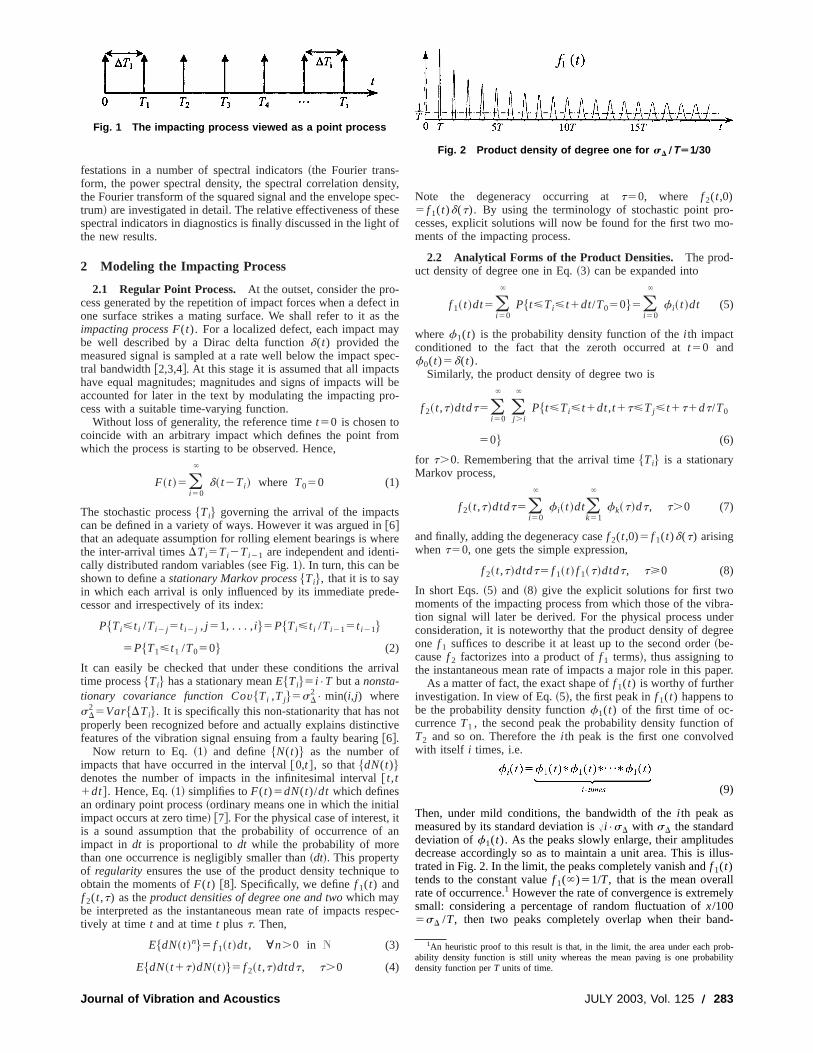
festations in a number of spectral indicators~the Fourier trans-form, the power spectral density, the spectral correlation density,the Fourier transform of the squared signal and the envelope spec-trum! are investigated in detail. The relative effectiveness of thesespectral indicators in diagnostics is finally discussed in the light ofthe new results.

2 Modeling the Impacting Process

2.1 Regular Point Process. At the outset, consider the pro-cess generated by the repetition of impact forces when a defect inone surface strikes a mating surface. We shall refer to it as theimpacting process F(t). For a localized defect, each impact maybe well described by a Dirac delta functiond(t) provided themeasured signal is sampled at a rate well below the impact spec-tral bandwidth@2,3,4#. At this stage it is assumed that all impactshave equal magnitudes; magnitudes and signs of impacts will beaccounted for later in the text by modulating the impacting pro-cess with a suitable time-varying function.

Without loss of generality, the reference timet50 is chosen tocoincide with an arbitrary impact which defines the point fromwhich the process is starting to be observed. Hence,

F~ t !5(i 50

`

d~ t2Ti ! where T050 (1)

The stochastic process$Ti% governing the arrival of the impactscan be defined in a variety of ways. However it was argued in@6#that an adequate assumption for rolling element bearings is wherethe inter-arrival timesDTi5Ti2Ti 21 are independent and identi-cally distributed random variables~see Fig. 1!. In turn, this can beshown to define astationary Markov process$Ti%, that it is to sayin which each arrival is only influenced by its immediate prede-cessor and irrespectively of its index:

P$Ti<t i /Ti 2 j5t i 2 j , j 51, . . . ,i %5P$Ti<t i /Ti 215t i 21%

5P$T1<t1 /T050% (2)

It can easily be checked that under these conditions the arrivaltime process$Ti% has a stationary meanE$Ti%5 i •T but anonsta-tionary covariance function Cov$Ti ,Tj%5sD

2• min(i,j) where

sD2 5Var$DTi%. It is specifically this non-stationarity that has not

properly been recognized before and actually explains distinctivefeatures of the vibration signal ensuing from a faulty bearing@6#.

Now return to Eq.~1! and define$N(t)% as the number ofimpacts that have occurred in the interval@0,t#, so that$dN(t)%denotes the number of impacts in the infinitesimal interval@ t,t1dt#. Hence, Eq.~1! simplifies toF(t)5dN(t)/dt which definesan ordinary point process~ordinary means one in which the initialimpact occurs at zero time! @7#. For the physical case of interest, itis a sound assumption that the probability of occurrence of animpact in dt is proportional todt while the probability of morethan one occurrence is negligibly smaller than~dt!. This propertyof regularity ensures the use of the product density technique toobtain the moments ofF(t) @8#. Specifically, we definef 1(t) andf 2(t,t) as theproduct densities of degree one and twowhich maybe interpreted as the instantaneous mean rate of impacts respec-tively at time t and at timet plus t. Then,

E$dN~ t !n%5 f 1~ t !dt, ;n.0 in N (3)

E$dN~ t1t!dN~ t !%5 f 2~ t,t!dtdt, t.0 (4)

Note the degeneracy occurring att50, where f 2(t,0)5 f 1(t)d(t). By using the terminology of stochastic point pro-cesses, explicit solutions will now be found for the first two mo-ments of the impacting process.

2.2 Analytical Forms of the Product Densities. The prod-uct density of degree one in Eq.~3! can be expanded into

f 1~ t !dt5(i 50

`

P$t<Ti<t1dt/T050%5(i 50

`

f i~ t !dt (5)

wheref1(t) is the probability density function of thei th impactconditioned to the fact that the zeroth occurred att50 andf0(t)5d(t).

Similarly, the product density of degree two is

f 2~ t,t!dtdt5(i 50

`

(j . i

`

P$t<Ti<t1dt,t1t<Tj<t1t1dt/T0

50% (6)

for t.0. Remembering that the arrival time$Ti% is a stationaryMarkov process,

f 2~ t,t!dtdt5(i 50

`

f i~ t !dt(k51

`

fk~t!dt, t.0 (7)

and finally, adding the degeneracy casef 2(t,0)5 f 1(t)d(t) arisingwhent50, one gets the simple expression,

f 2~ t,t!dtdt5 f 1~ t ! f 1~t!dtdt, t>0 (8)

In short Eqs.~5! and ~8! give the explicit solutions for first twomoments of the impacting process from which those of the vibra-tion signal will later be derived. For the physical process underconsideration, it is noteworthy that the product density of degreeone f 1 suffices to describe it at least up to the second order~be-causef 2 factorizes into a product off 1 terms!, thus assigning tothe instantaneous mean rate of impacts a major role in this paper.

As a matter of fact, the exact shape off 1(t) is worthy of furtherinvestigation. In view of Eq.~5!, the first peak inf 1(t) happens tobe the probability density functionf1(t) of the first time of oc-currenceT1 , the second peak the probability density function ofT2 and so on. Therefore thei th peak is the first one convolvedwith itself i times, i.e.

(9)

Then, under mild conditions, the bandwidth of thei th peak asmeasured by its standard deviation isA i •sD with sD the standarddeviation off1(t). As the peaks slowly enlarge, their amplitudesdecrease accordingly so as to maintain a unit area. This is illus-trated in Fig. 2. In the limit, the peaks completely vanish andf 1(t)tends to the constant valuef 1(`)51/T, that is the mean overallrate of occurrence.1 However the rate of convergence is extremelysmall: considering a percentage of random fluctuation ofx/1005sD /T, then two peaks completely overlap when their band-

1An heuristic proof to this result is that, in the limit, the area under each prob-ability density function is still unity whereas the mean paving is one probabilitydensity function perT units of time.

Fig. 1 The impacting process viewed as a point process

Fig. 2 Product density of degree one for sD ÕTÄ1Õ30


width is greater than their mutual spacing, that is whenA i •sD

.T or i .10000/x2. For random fluctuations of typically a fewpercent, this means it takes a few thousands peaks forf 1(t) toreach its limit.

Similarly, the product density of degree two can be verified totend to f 2(`,t)5 f 1(t)/T. This supports the assertion of refer-ence@6# where it was pointed out that the nonstationary impactingprocessF(t) ultimately tends to stationarity, yet so slowly that thephenomenon is hardly noticeable in practice over a finite time ofobservation.

2.3 Spectral Characteristics. Since most processing in-volved in the diagnosis of rolling element bearings is performed inthe Fourier domain, it is now necessary to derive the formulas forthe Fourier transforms of the product densitiesf 1(t) and f 2(t,t).

(a) Fourier Transform of the Product Density of Degree OneCombining Eq.~5! and Eq.~9!, the Fourier transform off 1(t) is

readily found to yield a continuous density,

F1~a!51

2p ERf 1~ t !e2 j a•tdt5@12F* ~a!#21 (10)

whereF~a! is the characteristic function of the first time of arrivalT1—or equivalently of the independent and identically distributedinter-arrival time process$DTi%. Equation ~10! is known as a‘‘renewal type’’ equation in the theory of stochastic processes, thestudy of which requires the exact knowledge of the probabilitylaw governingT1 . The Gamma law would probably be a goodcandidate here as it produces strictly positive inter-arrival timeswith a peaked probability around the mean valueT. Howeverwhen its variancesD

2 is small w.r.t. its meanT, the Gamma dis-tribution is well approximated by the Normal distribution with thesame mean and variance, thus making the calculations more trac-table. Under these assumptions,

F~a!'expS 21

2sD

2•a22 j a•t D (11)

from which Eq.~10! is readily found to yield a pole ata50 anda series of finite-energy peaks equi-spaced by 1/T, with maximaand minima respectively ona5k/T anda5k/T21/2,kPZ. Fig-ure 3 depicts the behavior of the modulusuF1(a)u where thepercentage of random fluctuationsD /T has been set rather largefor sake of demonstration. In contrast to the time domain, notefirstly ~i! that the magnitude of the peaks falls off more rapidly inthe Fourier domain and secondly,~ii ! that the bandwidth of thesuccessive peaks ofF1(a) remain more or less constant sincethey are bounded by 1/T.

(i) Fall off of the peaks. For sD2 !T, the relative magnitude of

the i th peak w.r.t. the first one decreases almost as fast as 1/i 2, thatis a slope of240 dB per decade. SinceF1(a) ultimately tendstowards a constant amplitude densityF1(`)51, this means thatthere exists a cut-off radian frequencyac'A2/sD after which allthe peaks have faded. Considering the percentage of random fluc-tuationx/1005sD /T, it is found thatF1(a) becomes almost con-stant afteri c522.5/x. For example, for a random fluctuation of2%, this means as few asi c511 peaks.

(ii) Quality factor. The ‘‘apparent increase’’ of the bandwidthresulting from the fall off of the peaks may be quantified by thequality factor Qi'T2/( i •p•sD)2 ~ratio of the maximum to theminimum of the i th peak!. This is naturally found to stronglydepend on the percentage of random fluctuationsD /T.

(b) Double Fourier Transform of the Product Density of De-gree Two

The formula forF1(a) can now be used to compute the doubleFourier transform off 2(t,t):

F2~a,v!51

4p2 E ER2

f 2~ t,t!e2 j a•te2 j v•tdtdt (12)

Distinguishing three casest,0, t50 andt.0 and after somealgebra, one finds

F2~a,v!5F1~a!•@F1~a!1F1~a2v!21# (13)

This defines a continuous spectral density with marked ridges run-ning along thev-variable and centered on alla5k/T, kPZ. Forlarge values ofv, F2(a,v) ultimately tends toF1(a) and thusresembles a pattern of parallel and horizontal ridges along thev-axis rapidly falling off on each side ofa50, as illustrated inFig. 4. The presence of these parallel ridges distinctively charac-terizes the~second-order! spectral signature of a random train ofimpact forces and consequently, that of a faulty rolling elementbearing. Moreover, the distance between the ridges indicates themean rate of occurrence of the fault, thus enabling its identifica-tion in the mechanical system.

2.4 Discussion. At this stage, it is instructive to reviewsome former models proposed in the literature in light of the de-rived results. Clearly, for the deterministic modelf 1(t) is a per-fectly periodic train of Dirac deltasXT(t) and f 2(t,t) a two-dimensional version of it, vizf 2(t,t)5XT(t)•XT(t). The sameapplies to their respective Fourier transforms, vizF1(a)51/T•X1/T(a) and F2(a,v)51/T2

•X1/T(a)•X1/T(v). The limita-tion of these formulas arises from the experimental evidence thatactual data do not haveline spectraespecially in the vicinity ofthe high frequency resonance where they are usually demodu-lated. On the other hand, the simplified stochastic model proposedby Randall & Antoni in@5# leads tof 1(t)5XT(t)* f1(t), that isa periodic train of Dirac delta functions low-pass filtered by theprobability functionf1(t). Therein f 2(t,t) turns out to be peri-odic and low-pass filtered in thet-variable while transient in thet-variable. These ‘‘low-pass filter’’ and ‘‘transient’’ effects give abetter explanation for thecontinuityof experimental spectra in the

Fig. 3 Fourier transform „modulus … of the product density ofdegree one for sD ÕTÄ1Õ30

Fig. 4 Double Fourier transform „modulus … of the product den-sity of degree two for sD ÕTÄ1Õ30


vicinity of a high frequency resonance@4#. The refined stochasticmodel proposed herein obviously leads to almost identical prop-erties, yet on the basis of more accurate physical considerations.Of particular concern are the facts thatf 1(t) and f 2(t,t) are nolonger periodic functions neither in thet nor in thet variables andthat the ‘‘low-pass filter’’ effect is now replaced by a rapid ‘‘fall-off’’ effect. In other words, the Fourier transformsF1(a) andF2(a,v) are now purely continuous functions in botha and v~except ata50) where all the former discrete lines~harmonics!have been replaced bydistributed peaks, gradually broadeningwith increase ina. Actually, this fact is always observable inenvelope spectra, and was one of the main reasons for modifyingthe stochastic model first mentioned in reference@5#.

3 Spectral Statistics of the Vibration SignalIn the preceding section, expressions were derived which de-

scribe the spectral signature of a train of pulses as produced by alocalized defect. This section now discusses how this spectral sig-nature is transformed after the impacts have propagated throughthe system, i.e. as it is likely to be measured on the bearing hous-ing by an accelerometer.

3.1 Response of a Rolling Element Bearing to a RandomTrain of Impacts. Following classical models, the vibration sig-nal produced by a faulty rolling element bearing may be viewedas the response of a linear system driven by the impacting processF(t) @2,7#. For this input-output relationship to be fully compre-hensive, we now show that the impulse response of the systemshould be time-varying and should also accommodate some de-gree of stochasticity.

At the outset, the impacting process should be modulated by aperiodic and positive functionA(t) to account for the variations inthe impact magnitudes as the defect enters and exits the load zone@2#. Some random modulation might be incorporated inA(t) dueto the dependence on the position and the number of the rollingelements in the load zone at timet, but also due to rolling and slipon possibly rough surfaces especially after a defect has appearedand spread to some extent.

Next, let us definer (t,t) the structural response at timet of thesystem subjected to an impulsed~t! at time t. In contrast to astatic structure, the impulse responser (t,t) of a rolling elementbearing is time-varying for a variety of physical reasons, the mostobvious of which being the variations in the transmission path asthe coordinates of the point of impact move w.r.t the location ofthe sensor, and the variations in the relative angle between theimpact forces and the axis of the sensor. For a system operating atconstant speed, these variations periodically affect the magnitude,the sign and the phase of the impulse responser (t,t) with aperiod depending on whether the defect lies on the inner race, theouter race or on a rolling element@2#. In addition, r (t,t) mighthave some small random fluctuations to account for unpredictableeffects such as contact non-linearities. Figure 5~a! gives a sche-matic illustration of how the impacting processA(t)F(t) is trans-formed into a vibrationX(t) after passing through the impulseresponser (t,t).

In practice, the vibration signalX(t) produced by a local faultcannot be observed totally because it is contaminated by othervibrations from a multitude of neighboring sources in the system.Therefore, it is customary to filter it in a frequency band where thesignal-to-noise ratio is maximum so that virtually no other sourcesthan that stemming from the faulty bearing are measured by theexperimenter. This is usually done by designing a band-pass filterb(t) around a high-frequency resonance of the structure~or thesensor! that is excited by the impacts@1–4#. In order to retain thediagnostic information, the band-pass filterb(t) must have thefollowing properties:

P1: b(t) is a band-pass filter with central frequencyv0 muchhigher than the mean rate of impacts1/T,

P2: b(t) has an effective duration shorter than the mean inter-arrival time T, or equivalently its spectral bandwidth is largerthan the mean rate of impacts1/T.

Therefore, the overall impulse response of the system is ob-tained from cascading the amplitude modulation functionA(t)with the time-varying impulse responser (t,t) and finally with theband-pass filterb(t). This is illustrated in Fig. 5~b!.

In this procedure,A(t) andg(t,t)5b(t2l)r (l,t) have someimportant properties which will make the computation of theinput-output relationship tractable. Specifically, becauseA(t) en-compasses all the periodic modulations with possible stochasticeffects, it has first and second-order statistics given by:

mA~ t !5E$A~ t !%5mAS t12p

V D5(kPZ

akej V•t (14)

and

RA~ t,t!5E$A~ t1t!A* ~ t !%5RAS t12p

V,t D5(

kPZRA

k ~t!ej V•t

(15)

Equations~14! and ~15! define asecond-order cyclostationaryprocess, i.e. a stochastic process with periodic mean and autocor-relation function of intrinsic period 2p/V. Therein V is eitherequal to the speed of the inner race, that of the outer race or thatof the cage~relative to the load vector! whether the fault is on theinner race, the outer race, or on a rolling element.

Similarly, g(t,t) being a periodic causal Green’s function de-scribing the periodically varying transmission path, it expandsinto:

g~ t,t!5H gS t12p

V,t D5(

kPZgk~ t2t!ej V•t, t<t

0 t.t

(16)

From the above expansion, the mechanism relating the impactingprocessF(t) to the band-pass vibration signalY(t) can finally beobtained from the following Stieltjes stochastic integral

Y~ t !5E0

t

g~ t,t!A~t!dN~t!5(kPZ

ej V•tERgk~ t2t!A~t!dN~t!

(17)

in which each Fourier coefficientgk(t) is to be interpreted as alinear, causal and homogeneous impulse response.

3.2 Spectral Characteristics of the Vibration Response.From Eq.~17!, the spectral characteristics of the band-pass vibra-tion signal can now be derived and applied to a number of poten-tial indicators for use in diagnostics, namely the Fourier transformof the expected signal, the power spectral density, the spectralcorrelation, the Fourier transform of the expected squared signaland the power spectral density of the squared signal.

(a) Fourier Transform of the Expected ResponseFrom Eqs.~1!, ~14! and ~17!, the expected value~ensemble

average! of the vibration signal is

mY~ t !5E$Y~ t !%5E0

t

g~ t,t!mA~t! f 1~t!dt (18)

from which the Fourier transform is found to be:

5MY~a!5

1

2p ERmY~ t !e2 j a•tdt5(

kPZMYk

~a2kV!

MYk~a!5Gk~a!•F1~a!

F1~a!5MA~a!* F1~a!5(l PZ

al•F~a2 lV!

(19)


whereGk(a) andMA(a) are respectively the Fourier transformsof gk(t) andmA(t). In view of Eq.~19!, MY(a) is a superpositionof shifted functionsMYk

(a); each of them being in turn con-structed from shifted and scaled replicas ofF1(a) and thenweighted by the frequency responseGk(a). The construction ofMY(a) results in amixed spectrum with a family of infinite-energy pseudo-harmonics arounda50, all equi-spaced by the ro-tation speedV. The number of these pseudo-harmonics directlydepends on the number of Fourier coefficients ing(t,t) andmA(t). Note that this specific pattern repeats around all the peaksof F1(a) at a5k/T, kPZ, but with finite-energy peaks in placeof pseudo-harmonics for anykÞ0. Obviously, this makes the verydistinctive ‘‘spectral signature’’ of a localized defect as it is ex-pected to appear in a faulty rolling element bearing~see Fig. 6!.Most importantly its detection forms the main basis of diagnosticssince it contains the key characteristic frequencies 1/T andV thatenable theidentificationand thelocalizationof faults in complexsystems.

However, the problem in the spectral indicator of Eq.~19! isthat the frequency support of the band-filtersGk(a) is very likelyto be higher than the frequency support of the spectral signatureF1(a) as shown schematically in Fig. 7. In fact, it was alreadypointed out thatF1(a) falls off by 240 dB per decade down to acut-off radian frequencyac of about&/sD . In order forGk(a)

to overlap with this support, its central radian frequencyv0 ~reso-nance frequency chosen for demodulation! should be such thatv0•T,100&/x with x/1005sD /T the percentage of fluctuation.Or equivalently, withi c the number of peaks inF1(a) before itdies to 1,v0 should be such thatv0•T,2p• i c . In most instancesthis condition would not be satisfied if a good signal-to-noise ratiowere to be maintained, thus justifying the poor performance an-ticipated from the Fourier transform of the vibration signal.

(b) Power Spectral Density of the ResponseFrom Eqs.~4!, ~15! and~17!, the autocorrelation function of the

vibration response is:

Fig. 5 „a… Generation of the resulting vibration signal. A „t …: magnitude of theimpacts; r „t ,t…: time-varying „stochastic … structural impulse response at time t .„b… Scheme of the overall impulse response. b „t… is a band-pass filter that ex-tracts the bearing signal where its signal-to-noise ratio is the highest

Fig. 6 Typical spectral signature in the vibration signal forsD ÕTÄ1Õ30 and VÄTÕ10


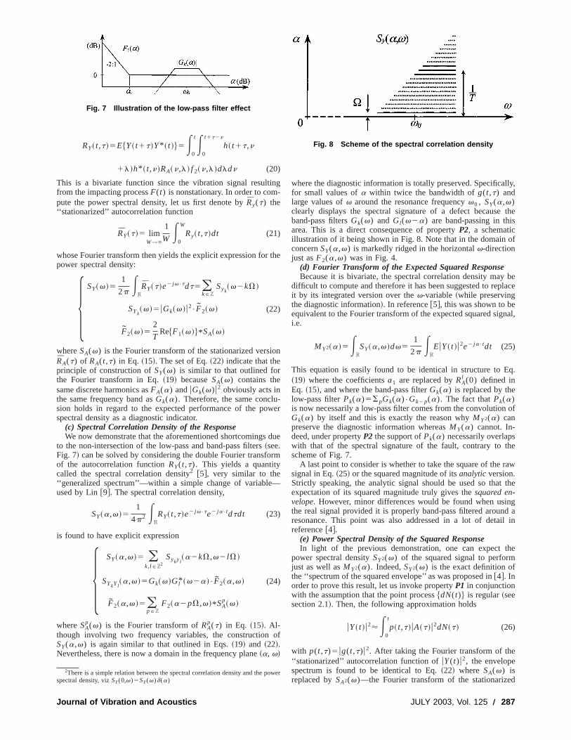
RY~ t,t!5E$Y~ t1t!Y* ~ t !%5E0

tE0

t1t2n

h~ t1t,n

1l!h* ~ t,n!RA~n,l! f 2~n,l!dldn (20)

This is a bivariate function since the vibration signal resultingfrom the impacting processF(t) is nonstationary. In order to com-pute the power spectral density, let us first denote byRy(t) the‘‘stationarized’’ autocorrelation function

RY~t!5 limW→`

1

W E0

W

Ry~ t,t!dt (21)

whose Fourier transform then yields the explicit expression for thepower spectral density:

5SY~v!5

1

2p ERRY~t!e2 j v•tdt5(

kPZSyk

~v2kV!

SYk~v!5uGk~v!u2

•F2~v!

F2~v!52

TRe$F1~v!%* SA~v!

(22)

whereSA(v) is the Fourier transform of the stationarized versionRA(t) of RA(t,t) in Eq. ~15!. The set of Eq.~22! indicate that theprinciple of construction ofSY(v) is similar to that outlined forthe Fourier transform in Eq.~19! becauseSA(v) contains thesame discrete harmonics asFA(a) anduGk(v)u2 obviously acts inthe same frequency band asGk(a). Therefore, the same conclu-sion holds in regard to the expected performance of the powerspectral density as a diagnostic indicator.

(c) Spectral Correlation Density of the ResponseWe now demonstrate that the aforementioned shortcomings due

to the non-intersection of the low-pass and band-pass filters~see.Fig. 7! can be solved by considering the double Fourier transformof the autocorrelation functionRY(t,t). This yields a quantitycalled the spectral correlation density2 @5#, very similar to the‘‘generalized spectrum’’—within a simple change of variable—used by Lin@9#. The spectral correlation density,

SY~a,v!51

4p2 ERRY~ t,t!e2 j v•te2 j a•tdtdt (23)

is found to have explicit expression

5SY~a,v!5 (

k,l PZ2Sykyl

~a2kV,v2 lV!

SYkYl~a,v!5Gk~v!Gl* ~v2a!•F2~a,v!

F2~a,v!5(pPZ

F2~a2pV,v!* SAp~v!

(24)

whereSAp(v) is the Fourier transform ofRA

p(t) in Eq. ~15!. Al-though involving two frequency variables, the construction ofSY(a,v) is again similar to that outlined in Eqs.~19! and ~22!.Nevertheless, there is now a domain in the frequency plane~a, v!

where the diagnostic information is totally preserved. Specifically,for small values ofa within twice the bandwidth ofg(t,t) andlarge values ofv around the resonance frequencyv0 , SY(a,v)clearly displays the spectral signature of a defect because theband-pass filtersGk(v) and Gl(v2a) are band-passing in thisarea. This is a direct consequence of propertyP2, a schematicillustration of it being shown in Fig. 8. Note that in the domain ofconcernSY(a,v) is markedly ridged in the horizontalv-directionjust asF2(a,v) was in Fig. 4.

(d) Fourier Transform of the Expected Squared ResponseBecause it is bivariate, the spectral correlation density may be

difficult to compute and therefore it has been suggested to replaceit by its integrated version over thev-variable~while preservingthe diagnostic information!. In reference@5#, this was shown to beequivalent to the Fourier transform of the expected squared signal,i.e.

MY2~a!5ERSY~a,v!dv5

1

2p EREuY~ t !u2e2 j a•tdt (25)

This equation is easily found to be identical in structure to Eq.~19! where the coefficientsa1 are replaced byRA

l (0) defined inEq. ~15!, and where the band-pass filterGk(a) is replaced by thelow-pass filterPk(a)5SpGk(a)•Gk2p(a). The fact thatPk(a)is now necessarily a low-pass filter comes from the convolution ofGk(a) by itself and this is exactly the reason whyMY2(a) canpreserve the diagnostic information whereasMY(a) cannot. In-deed, under propertyP2 the support ofPk(a) necessarily overlapswith that of the spectral signature of the fault, contrary to thescheme of Fig. 7.

A last point to consider is whether to take the square of the rawsignal in Eq.~25! or the squared magnitude of itsanalyticversion.Strictly speaking, the analytic signal should be used so that theexpectation of its squared magnitude truly gives thesquared en-velope. However, minor differences would be found when usingthe real signal provided it is properly band-pass filtered around aresonance. This point was also addressed in a lot of detail inreference@4#.

(e) Power Spectral Density of the Squared ResponseIn light of the previous demonstration, one can expect the

power spectral densitySY2(v) of the squared signal to performjust as well asMY2(a). Indeed,SY2(v) is the exact definition ofthe ‘‘spectrum of the squared envelope’’ as was proposed in@4#. Inorder to prove this result, let us invoke propertyP1 in conjunctionwith the assumption that the point process$dN(t)% is regular~seesection 2.1!. Then, the following approximation holds

uY~ t !u2'E0

t

p~ t,t!uA~t!u2dN~t! (26)

with p(t,t)5ug(t,t)u2. After taking the Fourier transform of the‘‘stationarized’’ autocorrelation function ofuY(t)u2, the envelopespectrum is found to be identical to Eq.~22! where SA(v) isreplaced bySA2(v)—the Fourier transform of the stationarized

2There is a simple relation between the spectral correlation density and the powerspectral density, vizSY(0,v)5SY(v)d(a)

Fig. 7 Illustration of the low-pass filter effect

Fig. 8 Scheme of the spectral correlation density


autocorrelation function RA2(t) of the squared process$uA(t)u2%—and whereuGk(v)u2 is replaced byuPk(v)u2. The factthat uPk(a)u2 acts as a low-pass filter demonstrates again thatSY2(v) is also a usable diagnostic indicator. Here again, the ana-lytic version of the signal may be preferred in Eq.~26! in order toestimate the power spectral density of the true squared envelope.

3.3 Discussion. It has been proven in some depth why theFourier transform and the power spectral density generally arepoor indicators for diagnosing rolling element bearings in the caseof localized faults, a fact that the authors have regularly observedon experimental data. Indeed, even though classical spectralanalysis may perform very well in detecting a fault—e.g. throughmonitoring the relative energy levels in some frequency bands—itrarely helps in recognizing its type nor its location—and this isexactly what diagnostics asks for. For example, Figure 9 comparesthe power spectral densities of a vibration signal measured on agearbox before and after one of the rolling element bearings~12balls,B7.12 mm, pitch circleB38.5 mm! was purposely damagedby machining a small slot on its inner race. The frequency reso-lution is 12 Hz. Note that the presence of the fault only shows upat high frequencies. The fact that there is no difference at lowfrequencies is due to the extremely poor signal-to-noise ratio inthat band~observe that most of the sources there relate to harmon-ics from the gears!. Of interest also is the fact that in spite of itsincrease, the spectral density at higher frequencies is continuousand therefore gives no indication of a fault producing repetitiveimpacts.

In clear contrast with the Fourier transform and the power spec-tral density, the same transformations applied on thesquaredsig-nal ~or its analytic version! have been shown to solve the problemin a surprisingly simple manner. For example, Fig. 10 displays thepower spectrum of the squared magnitude of the analytic signalafter band-pass filtering in the frequency [email protected]; 2.2# kHz witha frequency resolution of 2 Hz. Now the specific spectral signa-

ture of the inner race fault shows up in good accordance with Fig.4, with 1/T571 Hz ~ball pass frequency on the fault! and V510 Hz ~shaft rotation!.

From a theoretical point of view, it is worth mentioning that theFourier transform of the squared signal preserves the diagnosticinformation by exploiting the non-stationarity of the signal, whilethe power spectral density exploits its non-Gaussianity. In fact, thepower spectral density of the squared signal is implicitly a fourth-order ‘‘stationarized’’ statistic. Strictly speaking, these two indica-tors have different theoretical justifications and this is supportedby recalling that the former only requires propertyP2, while thelatter requires the more stringent conditionP21P1. However,both are inclined to provide envelope analysis—or ‘‘squared’’ en-velope analysis—with a strong formal justification.

Comparison of the five spectral indicators, which have beenassessed so forth, is summarized in Table 1.

4 ConclusionA comprehensive stochastic model has been proposed for de-

scribing and simulating the vibration produced by localized faultsin rolling element bearings. Sources of stochasticity were modeledin both the impacting force process—by means of a regular pointprocess—and in the transmission path—by means of a cyclosta-tionary process, thus encompassing a large range of physical situ-ations. These refinements proved very valuable in explainingsome of the actual features observed on experimental data. Thespectral signature of a localized fault was derived analytically andnew results were deduced concerning the nature of spectral har-monics produced by the impacting process. These were shown tobe distributed and equi-spaced~by the mean rate of impacts!peaks with arapid fall-off that could be quantified as a function ofthe percentage of stochastic fluctuations. Next, the spectral signa-ture of a defect was shown to duplicate when it propagatesthrough the structure~with shifts equal to the rotation speed of thedefect!, thus generating additional families of pseudo-harmonics.These results finally helped in investigating the effectiveness of anumber of spectral indicators dedicated to the diagnostics of roll-ing element bearings. From simple considerations on band-passand low-pass filtering operations, it was demonstrated that boththe Fourier transform and the power spectral density of thesquared signalare the most relevant indicators, thus bringing newsupports in favor of ‘‘squared’’ envelope analysis.

References@1# Darlow, M. S., and Badgley, R. H., 1975, ‘‘Applications for Early Detection of

Rolling Element Bearing Failures Using the High-Frequency Resonance Tech-nique,’’ ASME Paper 75-DET-46.

@2# McFadden, P. D., and Smith, J. D., 1984, ‘‘Model for the Vibration Producedby a Single Point Defect in a Rolling Element Bearing,’’ J. Sound Vib.,91~1!,pp. 69–82.

@3# McFadden, P. D., and Smith, J. D., 1985, ‘‘The Vibration Produced by Mul-tiple Point Defects in a Rolling Element Bearing,’’ J. Sound Vib.,98~2!, pp.69–82.

Fig. 10 Power spectral density of the squared envelope

Table 1 Comparison of five spectral indicators in terms oftheir ability of detecting and identifying localized faults.

Spectral indicators Diagnostic skills

Fourier transform of expected signal 2Power spectrum of the signal 2Spectral correlation density~2-D! of the signal 11Fourier transform of the expected squared signal 11Power spectrum of the squared signal 11

Fig. 9 Power spectral density of a vibration signal in case of no fault „continuous line … and aninner race fault „dotted line …


@4# Ho, D., and Randall, R. B., 2000, ‘‘Optimization of Bearing Diagnostics Tech-niques Using Simulated and Actual Bearing Fault Signals,’’ Mech. Syst. SignalProcess.,14~5!, pp. 763–788.

@5# Randall, R. B., Antoni, J., and Chobsaard, S., 2001, ‘‘The Relationship Be-tween Spectral Correlation and Envelope Analysis in the Diagnostics of Bear-ing Faults and other Cyclostationary Machine Signals,’’ Mech. Syst. SignalProcess.,15~5!, pp. 945–962.

@6# Antoni, J., and Randall, R. B., 2002, ‘‘Differential Diagnosis of Gear andBearing Faults,’’ ASME J. Vibr. Acoust.,127, pp. 1–7.

@7# Roberts, J. B., 1966, ‘‘On the Response of a Simple Oscillator to RandomImpulses,’’ J. Sound Vib.,4~1!, pp. 51–61.

@8# Srinivasan, S. K., et al., 1967, ‘‘Response of Linear Vibratory Systems toNon-Stationary Stochastic Impulses,’’ J. Sound Vib.,6~2!, pp. 169–179.

@9# Lin, Y. K., 1965, ‘‘Nonstationary Excitation and Response in Linear SystemsTreated as Sequences of Random Pulses,’’ J. Acoust. Soc. Am., pp. 453–460.


Nabeel ShabanehGraduate Student

Jean W. ZuAssociate Professor

Department of Mechanical & IndustrialEngineering,

University of Toronto,5 King’s College Road,

Toronto, Ontario, Canada, M5S 3G8

Nonlinear Dynamic Analysisof a Rotor Shaft System WithViscoelastically SupportedBearingsThis research investigates the dynamic analysis of a single-rotor shaft system with non-linear elastic bearings at the ends mounted on viscoelastic suspension. Timoshenko shaftmodel is utilized to incorporate the flexibility of the shaft; the rotor is considered to berigid and located at the mid-span of the shaft. A nonlinear bearing pedestal model isassumed which has a cubic nonlinear spring and linear damping characteristics. Theviscoelastic supports are modeled using Kelvin-Voigt model. Free and forced vibration isinvestigated based on the direct multiple scales method of one-to-one frequency-to-amplitude relationship using third order perturbation expansion. The results of the non-linear analysis show that a limiting value of the internal damping coefficient of the shaftexists where the trend of the frequency-response curve switches. Also, the primary reso-nance peak shifts to higher frequencies with the increase of the bearing nonlinear elasticcharacteristics, but with a flattened curve and hence lower peak values. A jump phenom-enon takes place for high values of the bearing nonlinear elastic characteristics.@DOI: 10.1115/1.1547684#

1 IntroductionAn effective means for controlling and reducing vibrations in

rotating machinery is the use of external damping and elastic el-ements often provided via flexible bearings and/or bearing sup-ports. Viscoelastic materials have emerged recently as externalmechanical dampers and bearing supports, offering simplicity indesign, operational enhancement and low cost in comparison withthe traditionally used squeeze film dampers@1#.

Modeling of the dynamic behavior of vibrating systems incor-porating viscoelastic elements has not been possible until recentlydue to the elaborate work of identifying the characteristic behav-ior of viscoelastic materials. Although there is much research onmodeling systems for structural applications, the work on rotatingshaft bearing systems mounted on viscoelastic supports is limited.In the few works reported on linear analysis, Dutt and Nakra@2–4# studied the stability and the unbalance vibration response ofa Jeffcott rotor system mounted on viscoelastic supports where adiscrete model of the shaft and linear elastic bearings were as-sumed. Using the finite element method based on the Euler-Bernoulli beam model, Kulkarni et al.@5# investigated the unbal-ance response and the stability of a rotating system withviscoelastically supported bearings. In further investigations, Sha-baneh and Zu@6–8# studied the dynamic behavior of a rotatingdisk-shaft system with linear elastic bearings at the ends mountedon viscoelastic supports. Timsohenko model was assumed for theshaft, and thus, the gyroscopic effect of the shaft was incorporatedin the analysis. Free and forced vibration analysis were carried outand the effects of the system characteristics were presented.Routh-Hurwitz criterion for polynomials with complex coeffi-cients and the variational analysis were used to perform the sta-bility analysis of the system. Furthermore, experimental investi-gations were performed to verify the obtained theoretical results.

Bearings in rotor shaft systems may possess nonlinear charac-teristics. For example, nonlinearity is inherent in ball bearings dueto Coulomb friction and the angular clearance between the roller

and the ring@9#. Ji and Zu@10# performed free and forced vibra-tion analysis to calculate natural frequencies for nonlinear rotorbearing system with cubic nonlinearity. However, incorporatingnonlinear bearing characteristics in rotor-shaft systems with vis-coelastic supports is very limited. A preliminary investigation wasreported by Bhattacharyya and Dutt@11#. They studied the unbal-anced response and stability of a rotor shaft system mounted onnonlinear rolling element bearings with viscoelastic supports. Theshaft was assumed to be massless with linear elasticity and inter-nal damping. In addition, the nonlinear restoring force of the bear-ings was linearized by the method of effective linearization, en-abling an approximate stability analysis using the Routh Hurwitzcriterion. The effects of gravity on the system and nonlinearitywere discussed. In the above work, the system was discretized andthe restoring force was approximated by a linear relation.

The aim of this research is to investigate the nonlinear dynamicbehavior of a continuous rotor shaft system with viscoelasticallysupported bearings. The nonlinearity occurs at the boundaries dueto nonlinear characteristics of the bearings. Timoshenko shaftmodel is used for the shaft, Kelvin Voigt model is utilized for theviscoelastic supports, and typical roller bearings with cubic non-linearity are employed. In the analysis, free and forced vibrationare developed based on the direct multiple scales method of one-to-one frequency-to-amplitude relationship of nonlinear systemusing the third order perturbation expansion. This approach doesnot require the selection of an orthogonal basis; however, it re-quires additional eigenfunction solutions at every level of approxi-mations. Moreover, the direct multiple scales method yields betterresults than the discretized one for finite mode truncations and forsystems having quadratic and cubic nonlinearities@12#. The re-sults of the nonlinear analysis indicate that a limiting value of theinternal damping coefficient of the shaft exists where the trend ofthe frequency-response curve switches. Also, a jump phenomenontakes place for high values of the nonlinear elastic coefficient ofthe bearings.

2 Equations of MotionConsider a continuous shaft-rotor system, as shown in Fig. 1,

where the frameoxyz is the inertial frame. A uniform shaft of

Contributed by the Technical Committee on Vibration and Sound for publicationin the JOURNAL OF VIBRATION AND ACOUSTICS. Manuscript received February2002; Revised October 2002. Associate Editor: G. T. Flowers.


length 2l is mounted on viscoelastically supported bearings. Therotor is considered as a rigid disk. For convenience, the viscoelas-tic element is represented by its equivalent complex stiffnessk*and is located at both ends of the shaft rotor system underneaththe bearings as support.

Adopting a continuous model of the shaft based on the Timosh-enko beam theory, and definingux , uy , cx , andcy as the trans-verse deflections along theox and oy directions and the corre-sponding bending angles in theoxz and oyz planes, respectively,the complex variablesu andc are assumed as

u5ux1 iuy , c5cx1 icy (1)

The general equations of motion of a uniform Timoshenko shaftsystem with internal damping are

rAu1@kAG~c2u8!#81Ci~ u2 iVu!50 (2)

rI sc2 iVJsc2~EIsc8!81kAG~c2u8!50 (3)

where (•)5Dt5]/]t and ( )85Dz5]/]z. A, I, Js andr are thecross-sectional area, transverse moment of inertia, polar mass mo-ment of inertia per unit length and mass density of the shaft.Ci isthe internal viscous damping coefficient andV is the spin rate ofthe shaft.E, G andk are Young’s modulous, shear modulous andshear coefficient, respectively.

The viscoelastic support is assumed to have a mass ofM2 andis modeled using Kelvin-Voigt model. Thus, the equivalent com-plex stiffness is defined ask* 5kv(11 ih). Denoting the displace-ments of the viscoelastic massM2 alongx andy directions byvxand vy , respectively, the complex deflection of the viscoelasticelement is given byv5vx1 ivy .

Introducing the nondimensional space variablez5z/ l , the re-lationship between the stress resultants and displacements in acomplex form are

M ~z,t !5Mx~z,t !1 iM y~z,t !5EIs

l

]c~z,t !

]z(4)

Q~z,t !5Qx~z,t !1 iQy~z,t !5kAGS 1

l

]u~z,t !

]z2c~z,t ! D (5)

whereM (z,t) andQ(z,t) are the transverse bending moment andthe shear force at each cross section along the shaft.

Due to symmetry of the system, only the left half of the rotor-shaft system, i.e., 0<z< l , is considered. Thus, the associatedboundary conditions can be defined as

M ~0,t !50 (6)

Q~0,t !5Fl~0,t !1Fn~0,t ! (7)

M2

]2v]t2 1kv~11 ih!v5Fl~0,t !1Fn~0,t ! (8)

Q~1,t !51

2 F2Md

]2u~1,t !

]t2 1MdeV2 exp~ iVt !G (9)

c~1,t !50 (10)

whereMd ande are the mass of the disk and the eccentricity ofthe rotor, respectively.Fl and Fn are the linear and nonlinearterms exerted by the bearings on the shaft and the viscoelasticsupports. Assuming that the bearings possess cubic nonlinear re-storing forces in addition to linear damping forces, the associatedforces are

Fl5Fxl1 iF yl5kb1~u2v !1cbS ]u

]t2

]v]t D (11)

Fn5Fxn1 iF yn5kb3@~ux2vx!31 i ~uy2vy!3# (12)

Equation~14! can be rewritten in terms of the complex trans-verse deflectionsu andv, and their corresponding complex con-jugatesu and v, as

Fn5kb3@34 ~u2u22uuv1v2u2u2v12uvv2v2v !

114 ~ u323u2v13uv22 v3!# (13)

Introducing a set of nondimensional quantities given in Appen-dix A, the nondimensional equations of motion with the associatedboundary conditions can be written as

]2u*

]t* 2 1]c*

]z2

]2u*

]z2 1Ci S ]u*

]t*2 iV* u* D50 (14)

]2c*

]t* 2 2 ia1V*]c*

]t*2a2

]2c*

]z2 1a3S c* 2]u*

]z D50 (15)

M* ~0,t !50 (16)

Q* ~0,t* !5kb1* ~u* 2v* !1cb* S ]u*

]t*2

]v*

]t* D1kb3* W* U~0,t* !

(17)

M2*]2v* ~0,t !

]t* 2 1kv* ~11 ih!v* ~0,t !

5kb1* ~u* 2v* !1cb* S ]u*

]t*2

]v*

]t* D1kb3* W* U~0,t* !

(18)

Q* ~1,t !521

2Md*

]2u* ~1,t !

]t* 2 11

2F* V* 2 exp~ iV* t* ! (19)

c* ~1,t !50 (20)

Fig. 1 Rotor shaft system with viscoelastically supportedbearings


3 Method of Multiple ScalesThe direct multiple scales method is used in this section to

solve for the free and forced vibration of the system. Expansionsof the displacementsu* , v* and the shear deformationc* areassumed as

u* 5«u1~z,T0 ,T2!1«3u3~z,T0 ,T2!1 . . . (21)

v* 5«v1~z,T0 ,T2!1«3v3~z,T0 ,T2!1 . . . (22)

c* 5«c1~z,T0 ,T2!1«3c3~z,T0 ,T2!1 . . . (23)

whereui , v i andc i ( i 51,3, . . . ) are oforderO(1), « is a smalldimensionless parameter, andTn5«nt* (n50,2, . . . ) is thenthorder time scale.T0 is a fast-time scale characterizing motionsoccurring at the spin rateV* and natural frequencyvn* of therotor bearing system;vn* 5vnAr l 2/kG. Furthermore,T2 is aslow-time scale characterizing the modulation of the amplitudeand phase due to nonlinearity, damping and resonance.

Considering the one-to-one primary resonance of the system,the damping forces, the forcing term and the excitation frequencyare assumed as

cb* 5«2cP , Ci* 5«2Ci P , F* 5«3FP , V* 5vn* 1«2s(24)

wheres5O(1) is a detuning parameter. The assumptions in Eq.~24! takes into account the interaction of damping terms with thenonlinear forces at the same level of approximation, which is anecessary condition for a nontrivial solution of the governingequations of motion. Thus, the effect of the nonlinearity of thesystem can be balanced with the effect of the system dampingat the same level of approximation, i.e., the third orderapproximation@13#.

The small dimensionless parameter« may take any value be-tween 0 and 1.0. However, by assuming a value of zero, the so-lution will be trivial. Moreover, in order to obtain a formal solu-tion of the equations of motion~14!–~20!, « should be equated to1.0. In such a case, it is stipulated that the nonlinear terms arethemselves small.

Using the chain rule for the partial derivatives with respect toboth time scalesT0 andT2 , substituting Eqs.~21!–~24! into Eqs.~14!–~20!, and equating coefficients of like power of«, the fol-lowing approximations of the system are obtained:Order«:

D02u11S ]c1

]z2

]2u1

]z2 D1Ci P~D0u12 ivn* u1!50 (25)

D02c12 ia1vn* D0c12a2

]2c1

]z2 1a3S c12]u1

]z D50 (26)

at z50

]c1

]z50, a3S ]u1

]z2c1D2kb1* ~u12v1!50, and

M2* D02v11kv* ~11 ih!v12kb1* ~u12v1!50 (27)

at z51

c150, a3S ]u1

]z2c1D1

Md*

2D0

2u150 (28)

Order«3:

D02u31

]c3

]z2

]2u3

]z2 1Ci P~D0u32 ivn* u3!

522D2D0u12Ci P~D2u12 isu1! (29)

D02c32 ia1vn* D0c32a2

]2c3

]z2 1a3S c32]u3

]z D522D2D0c11 ia1~vn* D2c11sD0c1! (30)

at z50

]c3

]z50, a3S ]u3

]z2c3D2kb1* ~u32v3!

5cPD0~u12v1!1kb3* W1 , and

M2* D02v31kv* ~11 ih!v32kb1* ~u32v3!

522M2* D0D2v11cPD0~u12v1!1kb3* W1 (31)

at z51

c350,

a3S ]u3

]z2c3D1

Md*

2D0

2u352Md* D2D0u1112 FPvn*

2

3exp~ i ~vn* 1«2s!t* ! (32)

where W1514 ~u1

2u122u1u1v11v12u12u1

2v112u1v1v12v12v1!

114 ~ u1

323u12v113u1v1

22 v13!.

3.1 First Order Equations. Noting that the equations ofmotion and the associated boundary conditions are linear at order«, the first order approximation of the deflections and deforma-tions can be assumed in the form

u1~z,t* !5A~T2!eivn* T0Yu~z!,

c1~z,t* !5A~T2!eivn* T0Yc~z!, v1~ t* !5A~T2!eivn* T0Yv(33)

Substituting Eq.~33! into Eqs.~25! and ~26! leads to a set ofordinary differential equations given by

a1Yu91a2Yu82a3Yc850 (34)

b1Yc91b2Yc82b3Yu850 (35)

where ( )85d/dz. The coefficients in Eqs.~34! and ~35! are de-fined as

a151, a25vn*2, a351 (36)

b15a2 , b25~12a1!vn*22a3 , b352a3 (37)

Decoupling Eqs.~34! and ~35! and assuming an exponentialsolution form forYu andYc yield the general solutions

Yu~z!5(j 51

4

Ajesjz, Yc~z!5(

j 51

4

Bjesjz (38)

wheresj ( j 51, . . . ,4) are theroots of the quartic auxiliary equa-tion @7#. Only four of the arbitrary complex constantsAj andBj( j 51, . . . ,4) are independent, since they are related by therelation

Bj5u jAj , u j5a1sj

21a2

a3sj~ j 51, . . . ,4! (39)

Substituting Eqs.~33! and ~38! into the boundary conditionEqs. ~27! and ~28! yields the eigenvalue problem represented inmatrix form as

@M ~vn* !# $Z%5$0% (40)

in which the eigenconstants are defined in vector notation as$Z%5@A1 A2 A3 A4 Yv#T, and the 535 coefficient matrix@M# isdefined as


m1k5a3~sj2a j !2kb1* m155kb1*

m2k5u j sj m2550

m3k52kb1* m3552M2* vn*21kv* ~11 ih!1kb1*

m4k5esj~a3~sj2u j !2Md* vn*2/2! m4550

m5k5u jesj m5550 ~k51, . . . ,4! (41)

To obtain the natural frequencyvn* , the determinant of thecoefficient matrix@M# must be zero. Considering that the coeffi-cient functionA(T2) in Eq. ~33! is arbitrary and assumingA151, the normal modesYu(z), Yc(z) andYv are uniquely definedby equation~40! for the eigenvaluevn* .

3.2 Third Order Equations. To achieve a third order solu-tion of the system, assume the complex displacementsu3 , c3 andv3 to be

u3~z,t* !5fu~z,T2!eivn* T0,

c3~z,t* !5fc~z,T2!eivn* T0,

v3~ t* !5fv~T2!eivn* T0 (42)

Substituting Eq.~42! into the set of Eqs.~29!–~32! yields

2]2fu

]z2 2vn*2fu1

]fc

]z

52~2ivn* 1Ci P!A8~T2!Yu~z!1 iCi PsA~T2!Yu~z!

(43)

2a2

]2fc

]z2 1~a121!vn*2fc1a3S fc2

]fu

]z D52 ivn* ~22a1!A8~T2!Yc~z!2a1vn* sA~T2!Yc~z!

(44)

at z50

]fc

]z50,

a3S ]fu

]z2fcD2kb1* ~fu2fv!

5cPivn* A~T2!~Yu~0!2Yv!13

4kb3* A2~T2!A~T2!W0 ,

and

2vn*2M2* fv1kv* ~11 ih!fv2kb1* ~fu2fv!

522ivn* M2* A8~T2!Yv1 ivn* cPA~T2!~Yu~0!2Yv!

134 kb3* A2~T2!A~T2!W0 (45)

at z51

fc50,

a3S ]fu

]z2fcD2

Md*

2vn*

2fu

52 ivn* Md* A8~T2!Yu~1!11

2FPvn*

2 exp~ isT2!

(46)

where ( )85]/]T2 , A(T2) is the complex conjugate of the coef-ficient A(T2), and W05Yu

3(0)23Yu2(0)Yv13Yu(0)Yv

22Yv3.

Note that the above terms in Eqs.~45! and~46! are collected onlyfor the primary resonance, i.e., exp(ivn*T0).

4 Solvability ConditionIn order to obtain a non-trivial solution for the homogeneous

part of Eqs.~43! and ~44!, the nonhomogeneous Eqs.~43! and~44! must satisfy a solvability or compatibility condition. As dis-cussed in@13#, the solvability condition demands that the righthand side of the nonhomogeneous equations be orthogonal to ev-ery solution of the corresponding adjoint homogeneous problem.

Since the corresponding homogeneous part of Eqs.~43! and~44! is self-adjoint, the solvability condition can be derived as

E0

1

$ua3@2~2ivn* 1Ci P!A8~T2!Yu~z!1 iCi PsA~T2!Yu~z!#

1c@2 ivn* ~22a1!A8~T2!Yc~z!2a1vn* sA~T2!Yc~z!#%dz

5$u~0,t* !@cPivn* A~T2!~Yu~0!2Yv!

134 kb3* A2~T2!A~T2!W0#2u~1,t* !

3@2 ivn* Md* A8~T2!Yu~1!112 FPvn*

2 exp~ isT2!#% (47)

whereu andc are the solutions of the adjoint homogeneous sys-tem of Eqs.~43! and ~44! and the boundary condition Eqs.~31!and ~32! with a zero right hand side.

It can be seen that the homogeneous adjoint system has anidentical form to the first order approximation given by Eqs.~25!–~28!; hence, the solutions foru, c and v should have the sameform asu1 , c1 andv1 .

Substituting the solutions ofu and c into Eq. ~47!, the solv-ability condition takes the compact form

b1~22ivn* 1Ci P!A8~T2!1b1iCi PsA~T2!

2b2ivn* ~22a1!A8~T2!2b2a1vn* sA~T2!

5cPivn* A~T2!~Yu2~0!2Yv

2!134 kb3* A2~T2!A~T2!W0Yu~0!

1 ivn* Md* A8~T2!Yu2~1!2

12 FPvn*

2 exp~ isT2!Yu~1! (48)

whereb15a3*01Yu

2(z)dz, b25a3*01Yc

2(z)dz, A is the complexconjugate of the coefficientA, andA8 is the derivative ofA withrespect to the slow time scaleT2 .

The coefficientA can be expressed in a polar form such that

A~T2!512 a~T2!e2 iu~T2! (49)

wherea(T2) andu(T2) represent the amplitude and phase angleof the response, respectively. To eliminate the explicit dependenceon T2 in the solvability condition and thus, transforming Eq.~48!from a nonautonomous system to an autonomous system, the newdependent variableg is introduced as

g5sT22u (50)


Substituting Eqs.~49! and ~50! into Eq. ~48! and separating thereal and imaginary parts, the modulation is given by

b3a81b4ag85b5as1b6a31b7a2FPvn*2Yu~1!cosg

(51)

2b4a81b3ag85b8as1b6a31b9a2FPvn*2Yu~1!sing

(52)

where the real coefficientsb3 , . . . ,b9 are defined in Appendix B.

5 Free Vibration ResponseThe free undamped frequencies of the nonlinear system can be

obtained by letting the quantitiesCi P , cP andFP equal to zero inEqs. ~51! and ~52!. Separating the variables and noting thatb75b950, Eqs.~51! and ~52! become

c1a81c2a1c3a350 (53)

u85b3

b4

a8

a2

b6

b4a21S 12

b5

b4Ds (54)

wherec15b421b3

2, c25(b8b42b5b3)s andc35b6b42b6b3 .Equations~53! and ~54! can be solved in conjunction with the

initial condition a5a0 andu5u0 at T250 to yield either of thefollowing three cases:Case 1:c2 /c3,0

a5A2c2~a121e22c2T2 /c1!/~c3a1

21c3e22c2T2 /c12c3! (55)

u~T2!5u01b3

b4H 1

2lnF a1

21e22c2T2 /c1

a121e22c2T2 /c121G J 2

1

2

b3

b4lnFa1

211

a12 G

1b6

b4

c1

2c3~a1221!

F ln~a121e22c2T2 /c121!

12a1

2c2

c1T22 ln a1

2G1S 12b5

b4DsT2 (56)

wherea125a0

2/(a021c2 /c3).

Case 2:c2 /c3,0

a5A2c2 /~c3a221c3e22c2T2 /c12c3! (57)

u~T2!5u02c1

2c3

b3

b4~a2221!

F ln~a221e22c2T2 /c121!

12c2

c1T22 ln a2

2G1b6

2b4@ ln~a2

21e22c2T2 /c121!2 ln a22#

1S 12b5

b4DsT2 (58)

wherea225(a0

22c2 /c3)/a02.

Case 3:c250

a5Aa02/~112c3a0

2T2 /c1! (59)

u~T2!5u02b3

2b4lnS 11

2c3

c1a0

2T2D2

c1

2c3

b6

b4lnS 11

2c3

c1a0

2T2D1S 12b5

b4DsT2 (60)

The frequency of the nonlinear systemvnn* is related to thefrequency of the linear systemvn* through the relation

vnn* 5vn* 1«2u8 (61)

whereu8 is the phase angle derivative with respect to the slowtime scaleT2 .

In a quasi-harmonic nonlinear system, the frequencies of thenonlinear system can be assumed periodic if the external forcing

terms and all the damping terms are eliminated. Such frequenciesare called free frequencies of the nonlinear system, and they aredependent among others on the initial conditions and strictly ap-plicable at steady state. However, these frequencies should not beconfused with the linear system natural frequencies.

6 Forced Vibration ResponseThe forced vibration of the system can be obtained by including

the damping terms,Ci P , cP and the forcing termFP in Eqs.~51!and~52!. To obtain the steady state response with periodic motion,the rate of change of the amplitude and the transformed phaseshift should be zero, i.e.,a85g850.

Eliminating the transformed phase shiftg from both of themodulation Eqs.~51! and ~52!, the detuning parameters can befound as a function of the amplitudea

s52b14

2b136

1

2b13Ab14

2 24b13b15 (62)

where the coefficients of the detuning parameterb13, b14 andb15are defined in Appendix C.

Equation~62! defines the frequency-response curve of the non-linear system, and each point on the curve corresponds to a spe-cific singular point on a state plane.

7 Numerical Results and DiscussionsNumerical simulations are performed for a typical rotor shaft

system with nonlinear bearings. The physical parameters of thissystem are given as

E52.0431011 Pa v50.3 r57750 kg/m3 l 50.15 m

Ci5200 kg/m.s ds50.0286 m k50.68 h50.01

kb1513109 N/m cb5400 kg/s kb3513107 N/m3

kv513109 N/m

M250.5 kg dd50.13 m Md555 kg e50.01 m

Assume that the shaft has a circular cross section, hencea152 andJs52rI s . In addition, the shaft rotates at a typical speedV5300 rad/s. Free and forced nonlinear vibration analysis arecarried out to this system to investigate the influence of nonlin-earity in the bearings on the system characteristic frequencies andfrequency response.

Figure 2 shows the free nonlinear oscillations of this system fordifferent values of the elastic coefficientkb3 of the nonlinear bear-ing. The initial transverse displacementu(0) is assumed as 10mm and the initial phase angleu0 is zero. The fundamental natu-ral frequency of the above system is 458.71 rad/s. It can be seenfrom the waveforms presented that increasing the nonlinearity ofthe system, i.e., increasingkb3 , shifts the frequency of the non-linear system to a higher value and increases the steady stateamplitude of the oscillation.

It is noted that the detuning parameters in the nonlinear freevibration analysis is related to the nondimensional spinning fre-quencyV* through the relations5(V* 2vn* )/«2. Also, the non-dimensional amplitudea can be related to the transverse deflec-tion of the shaft u at the first order approximation as

u(T0 ,T2 ,z)5« l /2a(T2)ei (vn* T02u(T2))Yu(z). This relation can besimplified for a zero initial phase angleu0 to become a52u/( l«).

Assuming that mass eccentricity of the disk has no contributionto the nonlinear forcing terms, the forcing termF* defined in Eq.~24! will be equal to zero, and subsequentlyFP will be equal tozero. The effect of the bearing nonlinear elastic coefficientkb3 onthe free frequency of the nonlinear system versus the amplitudeaof the transverse deflection is illustrated in Fig. 3. It is shown thatas the amplitude increases, the corresponding shift in the nonlin-ear natural frequency remains minimal for low values of the elas-


tic coefficientkb3 of the nonlinear bearing; i.e., for weak nonlin-ear system. Askb3 increases, the change in the natural frequencyof the nonlinear system increases significantly. The increase of thefrequencies of the nonlinear system and the bend of the curvetowards the higher frequencies are typical trends of hardeningnonlinearities.

Figures 4 and 5 show the effect of the internal viscous dampingcoefficientCi of the shaft on the free frequency of the nonlinearsystem versus amplitudes. Figure 4 depicts the trend for lowCivalues of 100 kg/m.s to 200 kg/m.s, whereas Fig. 5 shows thetrend for higherCi values of 270 kg/m.s to 300 kg/m.s. Figure 4shows that increasing the internal viscous damping of the shaftshifts the free frequency of the nonlinear system to higher valueswhile almost maintaining the curve characteristic. However, thistrend has a limiting value ofCi'270 kg/m.s beyond which anyincrease inCi will result in a shift of the curve to lower frequen-cies, as shown in Fig. 5. The limiting value of the internal damp-

ing coefficient,Ci'270 kg/m.s, indicates the increased efficiencyof the system to dissipate energy. This may be attributed to theoptimum interaction between the nonlinear restoring forces, exter-nal damping provided by the bearing supports and the viscoelasticelements, and the internal damping of the shaft.

It should be pointed out that since a zero forcing term corre-sponding to mass eccentricity of the disk is assumed for the re-sults of both Figs. 4 and 5, the free frequencies of the nonlinearsystem can be obtained. Also, the internal damping force is as-sumed to be linear; hence, proportional to the strain velocity,which is determined by the difference in whirling angular velocityand the rotational speed of the shaft. In general, the internal damp-ing force ~hysteretic damping! is nonlinear and roughly indepen-dent of the frequency. In addition, it is proportional to the squareof the vibration amplitude, to the shaft stiffness, and to the numberof reversals of the sign of the strain velocity@14#.

Including the effect of the mass eccentricity and hence the ex-

Fig. 2 Waveform of the transverse deflection for various values of bearingnonlinear elastic coefficient k b3

Fig. 3 Free frequency of the nonlinear system versus amplitudes for vari-ous values of bearing nonlinear elastic coefficient k b3


citation frequencyV, the steady-state frequency-response curve isshown near the primary resonance in Fig. 6. The effect of theelastic coefficientkb3 of the nonlinear bearing on the responsecurve is illustrated. Atkb3 equals zero, the response curve is iden-tical to the linear response curve. Askb3 increases, the responsecurve bends to the right side with lower and flattened peak. Thistrend continues until a jump phenomenon takes place due to themulti-valued phase points, indicating the bifurcation in the sys-tem. Also, for low values of the elastic coefficientkb3 (,13107 N/m3) of the nonlinear bearing, and thus weak nonlinearity,the frequency response curve deviates slightly from the frequencyresponse curve of the corresponding linear system.

It is worth noting that for large values of the nonlinear elasticcoefficientkb3 (.53108 N/m3), the perturbation analysis using

the multiple scales method starts to deviate from the basic as-sumption of weak nonlinearity. Thus, the error in predicting thefrequency response curves increases.

8 Summary and ConclusionsThe multiple scales method is adopted to analyze the free and

forced vibration of rotor shaft system with viscoelastically sup-ported nonlinear bearings. Timoshenko shaft model is assumed forthe shaft, two-element viscoelastic model is utilized for the sup-ports, and typical roller bearings with cubic nonlinearity are em-ployed. The free and forced vibration is developed based on thedirect multiple scales method. Third order perturbation expansionwith a one-to-one frequency-to-amplitude relationship of the non-

Fig. 4 Free frequency of the nonlinear system versus amplitudes for vari-ous values of internal viscous damping coefficient Ci of the shaft

Fig. 5 Free frequency of the nonlinear system versus amplitudes for highervalues of internal viscous damping coefficient Ci of the shaft


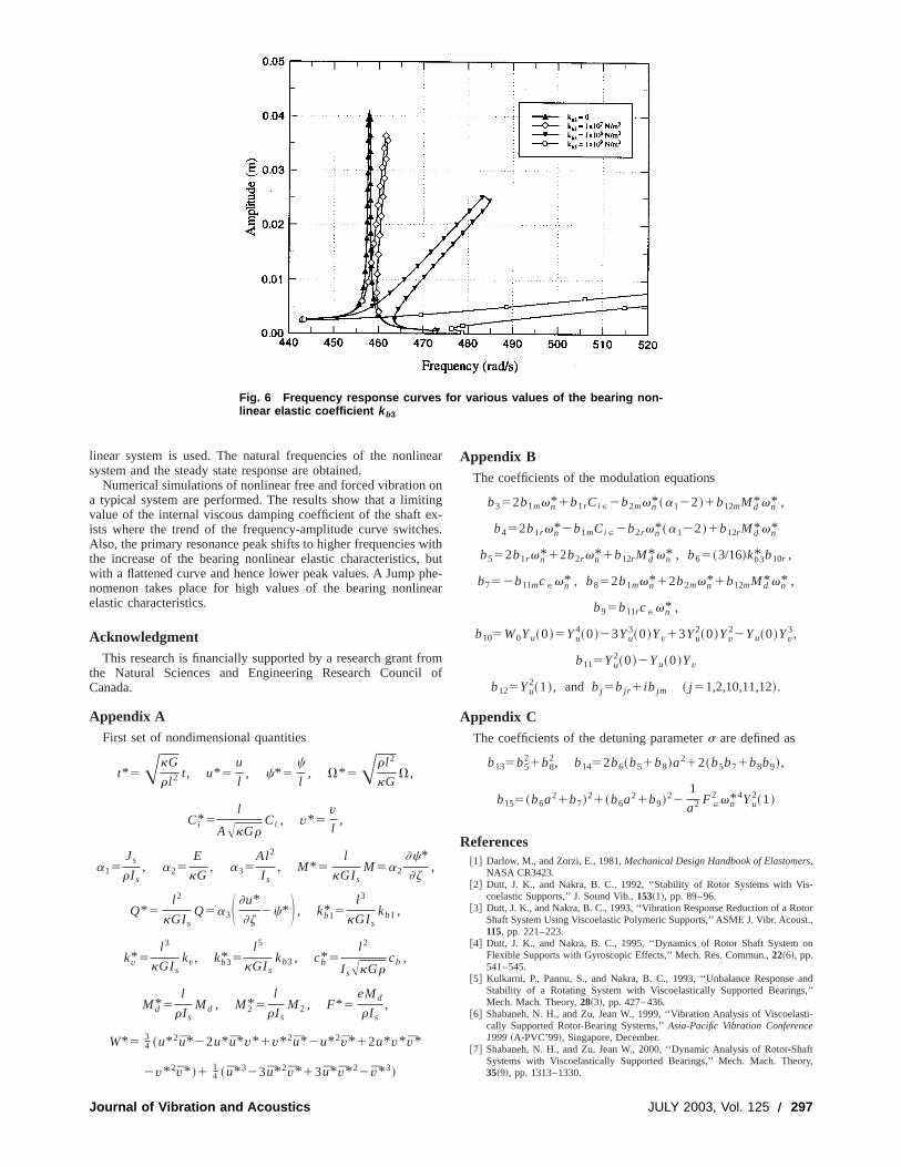
linear system is used. The natural frequencies of the nonlinearsystem and the steady state response are obtained.

Numerical simulations of nonlinear free and forced vibration ona typical system are performed. The results show that a limitingvalue of the internal viscous damping coefficient of the shaft ex-ists where the trend of the frequency-amplitude curve switches.Also, the primary resonance peak shifts to higher frequencies withthe increase of the bearing nonlinear elastic characteristics, butwith a flattened curve and hence lower peak values. A Jump phe-nomenon takes place for high values of the bearing nonlinearelastic characteristics.

AcknowledgmentThis research is financially supported by a research grant from

the Natural Sciences and Engineering Research Council ofCanada.

Appendix AFirst set of nondimensional quantities

t* 5AkG

r l 2 t, u* 5u

l, c* 5

c

l, V* 5Ar l 2

kGV,

Ci* 5l

AAkGrCi , v* 5

vl

,

a15Js

rI s, a25

E

kG, a35

Al2

I s, M* 5

l

kGIsM5a2

]c*

]z,

Q* 5l 2

kGIsQ5a3S ]u*

]z2c* D , kb1* 5

l 3

kGIskb1 ,

kv* 5l 3

kGIskv, kb3* 5

l 5

kGIskb3 , cb* 5

l 2

I sAkGrcb ,

Md* 5l

rI sMd , M2* 5

l

rI sM2 , F* 5

eMd

rI s,

W* 534 ~u* 2u* 22u* u* v* 1v* 2u* 2u* 2v* 12u* v* v*

2v* 2v* !114 ~ u* 323u* 2v* 13u* v* 22 v* 3!

Appendix BThe coefficients of the modulation equations

b352b1mvn* 1b1rCi P2b2mvn* ~a122!1b12mMd* vn* ,

b452b1rvn* 2b1mCi P2b2rvn* ~a122!1b12rMd* vn*

b552b1rvn* 12b2rvn* 1b12rMd* vn* , b65~3/16!kb3* b10r ,

b752b11mcPvn* , b852b1mvn* 12b2mvn* 1b12mMd* vn* ,

b95b11rcPvn* ,

b105W0Yu~0!5Yu4~0!23Yu

3~0!Yv13Yu2~0!Yv

22Yu~0!Yv3,

b115Yu2~0!2Yu~0!Yv

b125Yu2~1!, and bj5bjr 1 ib jm ~ j 51,2,10,11,12!.

Appendix CThe coefficients of the detuning parameters are defined as

b135b521b8

2, b1452b6~b51b8!a212~b5b71b8b9!,

b155~b6a21b7!21~b6a21b9!221

a2 FP2 vn*

4Yu2~1!

References@1# Darlow, M., and Zorzi, E., 1981,Mechanical Design Handbook of Elastomers,

NASA CR3423.@2# Dutt, J. K., and Nakra, B. C., 1992, ‘‘Stability of Rotor Systems with Vis-

coelastic Supports,’’ J. Sound Vib.,153~1!, pp. 89–96.@3# Dutt, J. K., and Nakra, B. C., 1993, ‘‘Vibration Response Reduction of a Rotor

Shaft System Using Viscoelastic Polymeric Supports,’’ ASME J. Vibr. Acoust.,115, pp. 221–223.

@4# Dutt, J. K., and Nakra, B. C., 1995, ‘‘Dynamics of Rotor Shaft System onFlexible Supports with Gyroscopic Effects,’’ Mech. Res. Commun.,22~6!, pp.541–545.

@5# Kulkarni, P., Pannu, S., and Nakra, B. C., 1993, ‘‘Unbalance Response andStability of a Rotating System with Viscoelastically Supported Bearings,’’Mech. Mach. Theory,28~3!, pp. 427–436.

@6# Shabaneh, N. H., and Zu, Jean W., 1999, ‘‘Vibration Analysis of Viscoelasti-cally Supported Rotor-Bearing Systems,’’Asia-Pacific Vibration Conference1999 ~A-PVC’99!, Singapore, December.

@7# Shabaneh, N. H., and Zu, Jean W., 2000, ‘‘Dynamic Analysis of Rotor-ShaftSystems with Viscoelastically Supported Bearings,’’ Mech. Mach. Theory,35~9!, pp. 1313–1330.

Fig. 6 Frequency response curves for various values of the bearing non-linear elastic coefficient k b3


@8# Shabaneh, N. H., and Zu, Jean W., 2000, ‘‘Dynamic and Stability Analysis ofRotor-Shaft Systems with Viscoelastically Supported Bearings,’’ Trans. Can.Soc. Mech. Eng.,24~1B!, pp. 179–189.

@9# Yamamoto, T., Yasuda, K., and Nagasaka, I., 1976, ‘‘Ultra-Subharmonic Os-cillations in a Nonlinear Vibratory System,’’ Bull. JSME,19~138!, pp. 1442–1447.

@10# Ji, Z., and Zu, J. W., 1998, ‘‘Method of Multiple Scales for Vibration Analysisof Rotor-Shaft Systems with Non-Linear Bearing Pedestal Model,’’ J. SoundVib., 218~2!, pp. 293–305.

@11# Bhattacharyya, K., and Dutt, J. K., 1997, ‘‘Unbalance Response and StabilityAnalysis of Horizontal Rotor Systems Mounted on Nonlinear Rolling Element

Bearings with Viscoelastic Supports,’’ ASME J. Vibr. Acoust.,119, pp. 539–544.

@12# Nayfeh, A. H., Nayfeh, J. F., and Mook, D. T., 1992, ‘‘On Methods for Con-tinuous Systems with Quadratic and Cubic Nonlinearities,’’ Nonlinear Dyn.3,pp. 145–162.

@13# Nayfeh, A. H., 1981,Introduction to Perturbation Techniques, Wiley, NewYork.

@14# Yamamoto, Toshio, and Ishida, Yukio, 2001,Linear and Nonlinear Rotordy-namics: A Modern Treatment with Applications, Wiley Series in NonlinearScience.


Animesh ChatterjeeAssistant Professor,

Department of Mechanical Engineering,Visvesvaraya National Institute of Technology,

Nagpur, India-440011e-mail: [email protected]

Nalinaksh S. VyasProfessor,

Department of Mechanical Engineering,Indian Institute of Technology,

Kanpur, India-208016e-mail: [email protected]

Nonlinear Parameter Estimationin Rotor-Bearing System UsingVolterra Series and Method ofHarmonic ProbingVolterra series provides a structured analytical platform for modeling and identification ofnonlinear systems. The series has been widely used in nonparametric identificationthrough higher order frequency response functions or FRFs. A parametric identificationprocedure based on recursive evaluation of response harmonic amplitude series is pre-sented here. The procedure is experimentally investigated for a rotor-bearing systemsupported in rolling element bearings. The estimates of nonlinear bearing stiffness ob-tained from experimentation have been compared with analytical values and experimentalresults of previous works.@DOI: 10.1115/1.1547486#

1 IntroductionSystem identification is an inverse problem of determination of

the mathematical structure of physical system from input-outputmeasurement. Volterra series provides a structured analytical plat-form for modeling and identification of nonlinear systems. Theseries represents nonlinear response through a set of multi-dimensional kernels, known as Volterra kernels. Fourier trans-forms of these kernels provide the definition of higher order ker-nel transforms, or higher order frequency response functions~FRFs! @1#. For harmonic excitations, the response can be conve-niently expressed in terms of the first and higher order FRFs.Extensive research work has been done in the area of non-parametric system identification through measurement of first andhigher order kernel transforms or FRFs. Boyd, Tang and Chua@2#developed a second order kernel transform measurement proce-dure using multi-tone harmonic probing. Chua and Liao@3# ex-tended the procedure for third and higher order kernel transforms.Gifford and Tomlinson@4# developed a multi-degree-of-freedomcurve fitting procedure for estimating the higher order FRFs.However, non-parametric system representation, in terms ofhigher order kernels, often requires extensive computational workand needs large number of experiments either with harmonic orstochastic excitation.

Parametric system identification requiresa-priori informationabout the topology of the mathematical structure of the system.Chatterjee and Vyas@5# have suggested an identification proce-dure for classification of systems between polynomial and non-polynomial form of nonlinearity. Further classification is madebetween symmetric and asymmetric forms of nonlinearity. For apolynomial form nonlinearity, the series structure is furtheridentified through a peak ratio comparison test under multi-toneexcitation.

Higher order FRFs, in case of polynomial form nonlinearity,can be synthesized with first order FRF and nonlinear parameters.This provides a generalized basis for nonlinear parameter estima-tion through measurement of first and higher order kernel trans-forms. Lee @6# extracted the response components of first har-monic through component separation technique. First and higherorder kernel transforms were then computed from the separatedresponse components and nonlinear parameters were estimatedusing the relationship between higher order and first order kernel

transforms. Chatterjee and Vyas@7# have suggested a recursiveiteration technique, which computes the first and higher order ker-nel transforms recursively from the measured response harmonicamplitudes. The response series is considered with an optimumnumber of terms governed by the convergence criterion.

In rotor-bearing systems, stiffness and damping nonlinearityplay a significant role in determining system behavior. Rollingelement bearing analyses presented by Harris@8# and Ragulskiet al. @9# point out that the stiffness force follows a symmetricnonlinearity relationship with deflection. Hydrodynamic bearingsoperating on fluid film lubrication also exhibit nonlinear relation-ship in the stiffness and damping forces. Investigations on rotorvibration, using nonlinear modeling of bearing coefficients, havebeen carried out by Bannister@10# and Choy et al.@11#. Garibaldiand Tomlinson@12# have presented a method for identifying thenonlinear bearing coefficients in a rigid rotor using Hilbert trans-form. Khan and Vyas@13# have developed parameter estimationprocedures for both rigid rotor and flexible rotor model. The pro-cedure employs Gaussian random excitation and Wiener kerneltransforms are extracted from the input-output data. Volterra ker-nel transforms are then obtained from the measured Wiener kerneltransforms and used for nonlinear parameter estimation.

The parameter estimation procedure described here employsharmonic probing technique in conjunction with Volterra seriesresponse representation. Investigation is carried out on a rotorsupported in rolling element bearings. The system is analyzed as asingle-degree-of-freedom system and linear and nonlinear stiff-ness parameters are estimated from the response measured at thebearing housing. The estimates are compared with theoretical val-ues obtained from the analytical work of Ragulski and also withsome earlier experimental results.

2 Volterra Series Response RepresentationVolterra series response for a general physical system withf (t)

as input excitation andx(t) as output response is represented by

x~ t !5x1~ t !1x2~ t !1x3~ t !1 . . . 1xn~ t !1 . . . (1)

with

xn~ t !5E2`

`

. . . E2`

`

hn~t1 , . . . ,tn! f ~ t2t1! . . . f ~ t

2tn!dt1 . . . dtn (2)

Contributed by the Technical Committee on Vibration and Sound for publicationin the JOURNAL OF VIBRATION AND ACOUSTICS. Manuscript received May 2002;revised October 2002. Associate Editor: M. I. Friswell.


hn(t1 , . . . ,tn) is the nth order Volterra kernel and its Fouriertransform provides thenth order frequency response functions~FRFs! or Volterra kernel transforms as

Hn~v1 , . . . ,vn!5E2`

`

. . . E2`

`

hn~t1 , . . . ,tn!

3)i 51

n

e2 j v it idt1 . . . dtn (3)

For a single-tone harmonic excitation

f ~ t !5A cosvt5A

2ej vt1

A

2e2 j vt (4)

the expression for thenth order response component, followingEq. ~2!, can be obtained as

xn~ t !5S A

2 D n

(p1q5n

nCqHnp,q~v!ej vp,qt (5)

where the following brief notations have been used

(5)The total response of the system, then becomes

x~ t !5(n51

` S A

2 D n

(p1q5n

nCqHnp,q~v!ej vp,qt (6)

The response series given in Eq.~6! can be written in terms of itsharmonics as

x~ t !5X01uX~v!ucos~vt1f1!1uX~2v!ucos~2vt1f2!

1uX~3v!ucos~3vt1f3!1.. (7)

where

X05(n51

` S A

2 D 2n2nCnH2n

n,n~v!

X~nv!5(i 51

`

s i~nv! and fn5/X~nv! (8)

with

s i~nv!52S A

2 D n12i 22n12i 22Ci 21Hn12i 22

n1 i 21,i 21~v! (9)

3 Parameter EstimationFor a system with polynomial form of nonlinearity under har-

monic excitation given by

mx~ t !1cx~ t !1k1x~ t !1k2x2~ t !1k3x3~ t !5A cosvt (10)

first three response harmonic series, after re-arranging and trun-cating Eq.~8! to a finite number of terms,k, can be expressed as

H1~v!'1

A FX~v!2(i 52

k

s i~v!G (11a)

H2~v,v!'2

A2 FX~2v!2(i 52

k

s i~2v!G (11b)

H3~v,v,v,!'4

A3 FX~3v!2(i 52

k

s i~3v!G (11c)

where the higher order kernel transforms are related to the lowerorder kernel transforms through nonlinear parameters~Chatterjeeand Vyas,@14#! as

Hnp,q~v!52

H1~vp,q!nCq F k2 (

pi1qi5nin11n25n

$n1Cq1Hn1

p1 ,q1~v!%* $n2Cq2Hn2

q2 ,q2~v!%1

k3 (pi1qi5ni

n11n21n35n

$n1Cq1Hn1

p1 ,q1~v!%* $n2Cq2Hn2

p2 ,q2~v!%* $n3Cq3Hn3

p3 ,q3~v!%G for n.1 (12)

Higher order series terms are initially neglected in Eqs.~11a–c!and kernel transformsH1(v), H2(v,v) andH3(v,v,v) are ex-tracted from measured harmonic amplitudes. Equation~12! is em-ployed to estimate the second and third order nonlinear param-eters k2 and k3 . Higher order series term contribution is thenconsidered and the procedure is iterated till the estimates convergewithin a specified limit. For a typical Duffing oscillator, the esti-mation algorithm can be structured through following steps.

Step-I: System is excited at frequencies,v i , with v i varyingover a frequency range including the natural frequency,vn , of thesystem. Responsex(t) is measured and harmonic amplitude,X(v i), is filtered to give preliminary estimate of first order kerneltransform as

H1~v i !5X~v i !/Ai , i 51, . . . .N (13)

The excitation levelAi is varied for constant response amplitudeX(v i) for keeping the series approximation error low and nearlyuniform over the frequency range@14#. Standard curve fitting pro-cedure~Ewins @15#! is employed to obtain the best fit FRF curveand preliminary estimation of linear parameters is made.

Step-II: System is excited at frequencies close to one-third ofnatural frequency, for distinct measurability of third harmonicX(3v) ~Ref. @14#!. Employing Eq.~12!, preliminary estimate ofnonlinear parameter,k3 , is obtained through regression betweenthe estimated third order kernel transform and its synthesized ker-nel factor,G3(v), using the following relationship

H3~v,v,v!5k3G3~v! (14)

where

G3~v!52H13~v!H1~3v! (15)

Step-III: The series( i 52k s i(v) is computed with theH1(v)

values taken from the best fit curve estimated in Step-I and thenonlinear parameter,k3 , estimated in Step-II and substituted inequation~11a! to obtain new estimates of linear parameters.

Step-IV:The series( i 52k s i(3v) is computed and substituted in

Eq. ~11c! to refine the estimate of the nonlinear parameterk3 .Iteration is continued till the estimate of nonlinear parameter,k3 ,converges within a specified limit.


The sign of the nonlinear parameter,k3 , is identified throughobservations of change of sign of real part of measured third har-monic amplitudes during transition of excitation frequency acrossone-third of the natural frequency. From Eqs.~14!, ~15!, one cannote that forv,vn/3, bothH1(v) andH1(3v) have positive realparts, which means that the kernel factorG3(v) will have a nega-tive real part. Consequently, the third order kernel transformH3(v,v,v) will also have a negative real part for positivek3 .For vn.v.vn/3, H1(v) will have a positive real part while thereal part ofH1(3v) will bear negative sign. The kernel factor,G3(v), andH3(v,v,v) will have a positive real part for positivevalue of the nonlinear parameterk3 .

4 Experimental Investigation

Experimental studies have been carried out on a test rig~Fig. 1!consisting of a 10 mm diameter shaft supported in ball bearings~SKF 6200!. A single-degree-of-freedom model is considered andcross-coupling stiffness parameters are neglected. Harmonic exci-tation force is applied on the bearing housing~in vertical direc-tion! through an electro-dynamic shaker. Measurement for excita-tion force and resultant vibration are made at the bearing housingthrough an impedance head attached between the shaker and bear

Fig. 1 „a… Experimental set up along with instrumentation „b…Close up view of exciter mounting arrangement and impedancehead

Fig. 2 Schematic diagram of rotor bearing test rig and instrumentation

Fig. 3 Response acceleration spectrum from rap test


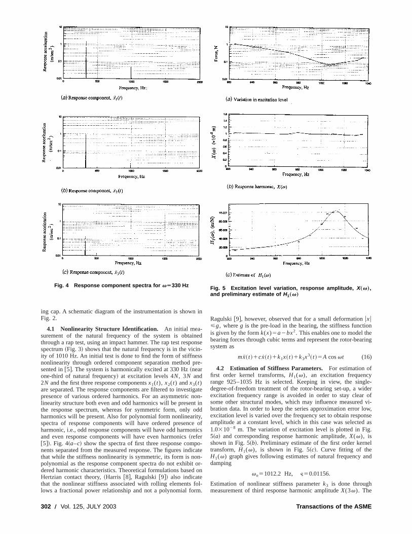
ing cap. A schematic diagram of the instrumentation is shown inFig. 2.

4.1 Nonlinearity Structure Identification. An initial mea-surement of the natural frequency of the system is obtainedthrough a rap test, using an impact hammer. The rap test responsespectrum~Fig. 3! shows that the natural frequency is in the vicin-ity of 1010 Hz. An initial test is done to find the form of stiffnessnonlinearity through ordered component separation method pre-sented in@5#. The system is harmonically excited at 330 Hz~nearone-third of natural frequency! at excitation levels 4N, 3N and2N and the first three response componentsx1(t), x2(t) andx3(t)are separated. The response components are filtered to investigatepresence of various ordered harmonics. For an asymmetric non-linearity structure both even and odd harmonics will be present inthe response spectrum, whereas for symmetric form, only oddharmonics will be present. Also for polynomial form nonlinearity,spectra of response components will have ordered presence ofharmonic, i.e., odd response components will have odd harmonicsand even response components will have even harmonics~refer@5#!. Fig. 4~a–c! show the spectra of first three response compo-nents separated from the measured response. The figures indicatethat while the stiffness nonlinearity is symmetric, its form is non-polynomial as the response component spectra do not exhibit or-dered harmonic characteristics. Theoretical formulations based onHertzian contact theory,~Harris @8#, Ragulski @9#! also indicatethat the nonlinear stiffness associated with rolling elements fol-lows a fractional power relationship and not a polynomial form.

Ragulski@9#, however, observed that for a small deformationuxu<g, whereg is the pre-load in the bearing, the stiffness functionis given by the formk(x)5a2bx2. This enables one to model thebearing forces through cubic terms and represent the rotor-bearingsystem as

mx~ t !1cx~ t !1k1x~ t !1k3x3~ t !5A cosvt (16)

4.2 Estimation of Stiffness Parameters. For estimation offirst order kernel transforms,H1(v), an excitation frequencyrange 925–1035 Hz is selected. Keeping in view, the single-degree-of-freedom treatment of the rotor-bearing set-up, a widerexcitation frequency range is avoided in order to stay clear ofsome other structural modes, which may influence measured vi-bration data. In order to keep the series approximation error low,excitation level is varied over the frequency set to obtain responseamplitude at a constant level, which in this case was selected as1.031028 m. The variation of excitation level is plotted in Fig.5~a! and corresponding response harmonic amplitude,X(v), isshown in Fig. 5~b!. Preliminary estimate of the first order kerneltransform, H1(v), is shown in Fig. 5~c!. Curve fitting of theH1(v) graph gives following estimates of natural frequency anddamping

vn51012.2 Hz, §50.01156.

Estimation of nonlinear stiffness parameterk3 is done throughmeasurement of third response harmonic amplitudeX(3v). The

Fig. 4 Response component spectra for vÄ330 Hz Fig. 5 Excitation level variation, response amplitude, X„v…,and preliminary estimate of H1„v…


displacement amplitude of the third response harmonic is low andtherefore measurements were made for acceleration amplitudes.Figure 6~a! shows the acceleration amplitudes of the first and thirdorder harmonics, for an excitation frequency of 330 Hz~near one-third natural frequency!. The ratio between the amplitudes at thirdharmonic and first harmonic is defined as measurability index,which provides the basis of selecting the excitation level and fre-quency range for measurement of third response harmonic ampli-tude X(3v). For measurement of third harmonic one can selectexcitation level corresponding to a certain measurability index.Figure 6~b! shows measurability indices for three different excita-tion amplitudes of 2N, 3N and 4N over a frequency range of 305Hz–355 Hz. Corresponding peak measurability indices can beseen to be approximately of the order of 3%, 5% and 10%. Exci-tation frequencies are selected at 330 Hz, 335 Hz, 340 Hz and 345Hz, as measurability is relatively higher in this range. Third re-sponse harmonic amplitudeX(3v) is then measured at these se-lected frequencies for three different excitation levels asCase I: Excitation level54 NCase II: Excitation level53 NCase III: Excitation level52 NFor case I corresponding to 10% measurability, the measured re-sponse acceleration spectra at the four selected frequencies areshown in Fig. 7~a–d!. A preliminary estimate of nonlinear param-eter k3 is made and the iteration procedure is repeated till esti-mated value of the nonlinear parameter converges within a limit,which in this case is specified as 0.1%. Figure 8~a! shows theestimated values of nonlinear parameterk3 over the stages ofsuccessive iteration. Final estimate ofk3 is found to be 1.75

31019 N/m3. Assuming that both the bearings are identical andact in parallel, the nonlinear stiffness parameter of each bearingthen becomes 0.87531019 N/m3. Figure 8~b! shows the final es-timate of the first order kernel transform along with its prelimi-nary estimate. It is seen that the successive iterations have im-proved the FRF values significantly near and around the naturalfrequency. Final estimates of natural frequency and damping be-come

vn51011.47 Hz, §50.01078.

The linear stiffness parameter,k1 , of the bearing system is com-puted from the natural frequency and the equivalent rotor massper bearing and is found to be 1.5853107 N/m.

Similar exercises are carried out with excitation level of 3N~Case II! and 2N ~Case III! corresponding to 5% and 3% mea-surability respectively. The convergence trend in the estimatek3 isshown respectively in Fig. 9~a, b!. The estimates of nonlinearstiffness parameter of each bearing is found to be 1.428531019 N/m3 ~Case II! and 1.74031019 N/m3 ~Case III! respec-tively. Damping and linear stiffness parameter are found as

Case II: §50.01015 k151.5353107 N/m.

Case III §50.01002 k151.5863107 N/m

The estimates for different cases are summarized in Table 1 givenbelow.

It can be seen from the estimates that, while the values of theestimated linear parameters are very accurate, the estimate of thenonlinear parameterk3 , varies with the excitation amplitude. Thisis due to the fact that the system nonlinearity does not adhere topolynomial form and therefore the cubic coefficient of equivalentpolynomial form would be amplitude dependent.

Figure 10 shows the sign variation of real part ofX(3v), overthe excitation frequency range 330–345 Hz for excitation levels4N, 3N and 2N. The sign of real part ofX(3v) is seen to changefrom positive values to negative values during frequency transi-tion through one-third natural frequency. This indicates that thenonlinearity is negative in sign.

5 Validation of EstimatesFor validation of the experimentally estimated nonlinear stiff-

ness parameter, analytical formulations of Harris@8# and Ragulskiet al. @9# are employed. These formulations are based on Hertz’stheory of elastic contacts and treat the bearings in isolation of theshaft. Figure 11 shows a typical isolated ball bearing configura-tion, in which external forces act alongx-axis. h i is the anglebetween load axis~i.e.,x-axis! and the radial direction of a typicali th ball element. For a displacement~x, y! of the moving ringalong the respective axes, total elastic force acting in radial direc-tion at the point of contact ofi th ball is given by

Fi5kn~g1x cosh i1y sinh i !3/2 (17)

and its projections alongx andy axes respectively are

Fxi5kn~g1x cosh i1y sinh i !3/2 cosh i (18)

Fyi5kn~g1x cosh i1y sinh i !3/2 sinh i (19)

whereg is the radial pre-load between the ball and the races,kn isa coefficient of proportionality depending on the geometric andmaterial properties of the bearing. Total restoring force of thebearing is equal to sum of elastic forces of all the elements,

i.e., F5(i 51

n

Fxi (20)

wheren is the number of rolling elements in the bearing in theloading zone.

Fig. 6 „a… Typical response spectrum with excitation at vÄ330 Hz „b… Measurability of third response harmonic at differ-ent excitation levels


Using the condition of zero elastic force alongy-axis ~since noexternal force acts along this axis! and following Eq.~19!, defor-mationy is obtained as

y5

(i 51

n

@g1x cosh i #3/2 sinh i

(i 51

n

@g1x cosh i #1/2 sin2 h i

(21)

Equations~18! and ~21! are used in Eq.~20! and the bearingstiffness is determined as a function of deformationx as

k~x!5]F/]x (22)

Substituting Eq.~20! in Eq. ~22!, taking into account Eq.~21! thebearing stiffness is expressed as a function of deformation as

k~x!5Kn(i 51

n

@g1x cosh i2~A/Bn!sinh i #1/2@cosh i2$CBn

2AD~n21!%/~Bn!2 sinh i #cosh i (23)

where

A5(i 51

n

@g1x cosh i #3/2 sinh i ; B5(

i 51

n

@g1x cosh i #3/2 sin2 h i

C5(i 51

n

@g1x cosh i #3/2 sinh i cosh i

(24)

D5(i 51

n

@g1x cosh i #3/2 sin2 h i cosh i

It can be seen that the bearing stiffness is critically dependent onthe pre-load. Table 2 summarizes the theoretical bearing stiffnessparameters for different pre-load along with experimentally ob-tained stiffness parameters. The stiffness variations are also shownin Fig. 12 along with experimental results of earlier researchers.

6 ConclusionThe stiffness parameter estimates from the experiment show

reasonably good agreement with those from available analyticalformulations for isolated ball bearings. The analytical formulationis dependent on the amount of preload and hence exact compari-

Fig. 7 Acceleration response spectra for Case I: Excitation amplitude Ä4 N


Fig. 8 „a… Iterative estimates of k 3 , „Case I: Excitationamplitude Ä4 N… „b… Final estimate of first order kernel trans-form, H1„v… „Case I: Excitation amplitude Ä4 N…

Fig. 9 „a… Iterative estimates of k 3 , „Case II: Excitationamplitude Ä3 N… „b… Iterative estimates of k 3 , „Case III: Excita-tion amplitude Ä2 N…

Fig. 10 Variation in sign of real part of X„3v… around vn Õ3 Fig. 11 Schematic diagram of a loaded ball bearing

Table 1 Linear and nonlinear estimates at different measur-ability cases

Nonlinear parameterk3 (31019 N/m3)

Naturalfrequency

Linear stiffnessk1 (3107 N/m) Damping

Case I: 4N 0.8750 1011.47 Hz 1.585 0.01078Case II: 3N 1.4285 1012.47 Hz 1.535 0.01015Case III: 2N 1.7400 1011.90 Hz 1.586 0.01002


son of theoretical values with experimental estimates is difficult.While, the manufacturer, at times may provide the preload range,the exact value of preloading of the bearing balls in the shaft-casing assembly, especially during operations which have in-volved wear and tear, would be difficult to determine. The sug-gested procedure gives good estimates of nonlinear parameter aswell as damping. The method is based on the assumption of linearviscous damping model. It can however be extended for identifi-cation and estimation of damping nonlinearity.

AcknowledgmentThe authors wish to express their thanks to the financial aid

being provided by the Propulsion Panel of Aeronautical Researchand Development Board, Ministry of Defense, Government of In-dia, in carrying out the study.

Nomenclature

Hn(v1 , . . . ,vn) 5 nth order Volterra kernel transformX(nv) 5 response amplitude ofnth harmonic

c 5 damping coefficientf (t) 5 excitation force

g 5 bearing pre-loadhn(t1 , . . . ,tn) 5 nth order Volterra kernel

k1 5 linear stiffness parameterk2 5 square non-linear stiffness parameterk3 5 cubic non-linear stiffness parameterm 5 mass of the system

xn(t) 5 nth order response componentG3(v) 5 Third order synthesized kernel factor

§ 5 damping factors i(nv) 5 i th term in the response harmonic series,

X(nv)

References@1# Bedrosian, E., and Rice, S. O., 1971, ‘‘The Output Properties of Volterra Sys-

tems ~Nonlinear System with Memory! Driven by Harmonic and GaussianInput,’’ Proc. IEEE,59~12!, pp. 1688–1707.

@2# Boyd, S., Tang, Y. S., and Chua, L. O., 1983, ‘‘Measuring Volterra Kernels,’’IEEE Trans. Circuits Syst.,CAS-30~8!, pp. 571–577.

@3# Chua, L. O., and Liao, Y., 1989, ‘‘Measuring Volterra Kernels~II !,’’ Int. J. ofCircuit Theory and Applications,17, pp. 151–190.

@4# Gifford, S. J., and Tomlinson, G. R., 1989, ‘‘Recent Advances in the Applica-tion of Functional Series to Nonlinear Structures,’’ J. Sound Vib.,135~2!, pp.289–317.

@5# Chatterjee, A., and Vyas, N. S., 2001, ‘‘Stiffness Nonlinearity Classificationthrough Structured Response Component Analysis using Volterra Series,’’Mech. Syst. Signal Process.,15~2!, pp. 323–336.

@6# Lee, G. M., 1997, ‘‘Estimation of Nonlinear System Parameters using HigherOrder Frequency Response Functions,’’ Mech. Syst. Signal Process.,11~2!, pp.219–228.

@7# Chatterjee, A., and Vyas, N. S., 2002, ‘‘Nonlinear Parameter Estimationthrough Volterra Series using Method of Recursive Iteration,’’ accepted forpublication in J. Sound Vib.

@8# Harris, T. A., 1984,Rolling Bearing Analysis, Wiley, New York.@9# Ragulskis, K. M., Jurkauskas A. Y., Atstupenas, V. V., Vitkute, A. Y., and

Kulvec, A. P., 1974,Vibration in Bearings, Mintis Publishers, Vilnius.@10# Bannister, R. H., 1976, ‘‘A Theoretical And Experimental Investigation Illus-

trating the Influence of Nonlinearity and Misalignment on the Eight Film Co-efficients,’’ Proc. Inst. Mech. Eng.,190, pp. 271–278.

@11# Choi, F. K., Braun, M. J., and Hu, Y., 1992, ‘‘Nonlinear Transient and Fre-quency Response Analysis of a Hydrodynamic Bearing,’’ ASME J. Tribol.,114, pp. 448–454.

@12# Garibaldi, L., and Tomlinson, G. R., 1988, ‘‘A Procedure for Identifying Non-linearity in Rigid Rotors Supported in Hydrodynamic and Ball/Roller BearingSystem,’’ I. Mech. Proc. on Vibrations in Rotating Machinery,4, pp. 229–234.

@13# Khan, A. A., and Vyas, N. S., 2001, ‘‘Application of Volterra and WienerTheories for Nonlinear Parameter Estimation in a Rotor-Bearing System,’’Nonlinear Dyn.,24~3!, pp. 285–304.

@14# Chatterjee, A., and Vyas, N. S., 2000, ‘‘Convergence Analysis of VolterraSeries Response of Nonlinear Systems Subjected to Harmonic Excitations,’’ J.Sound Vib.,236~2!, pp. 339–358.

@15# Ewins, D. J., 1984,Modal Testing: Theory and Practice, Research StudiesPress, England.

@16# Tiwari, R., and Vyas, N. S., 1995, ‘‘Estimation of Nonlinear Stiffness Param-eters of Rolling Element Bearings from Random Response of Rotor BearingSystems,’’ Journal of Sound Vib.187 ~2!, pp. 229–239.

Fig. 12 Comparison of estimates of stiffness parameters 1–5:Theoretical values with pre-load 0.2, 0.3, 0.4, 0.5 and 0.6 mmrespectively. †Harris †8‡ and Ragulski et al. †9‡ 6,7,8: Presentexperimental estimates for cases I, II and III respectively. 9: Ex-perimental estimate of Tiwari †16‡ 10: Experimental estimate ofKhan †13‡

Table 2 Estimated and theoretical „Ragulskis et al. †9‡; Harris, †8‡… bearing stiffnessparameters

Theoretical Stiffness~N/m! Estimated Stiffness~N/m!Pre-load~mm! k(x) from equation~22! (k123k3x2)

0.2 1.20310724.0131019x2 Case i!: 1.585310722.62531019x2

0.3 1.47310722.1831019x2 Case ii!: 1.535310724.28531019x2

0.4 1.69310721.4231019x2 Case iii!: 1.586310725.24031019x2

0.5 1.89310721.0231019x2

0.6 2.08310720.6131019x2


Y. S. Ho

H. Liu

Department of Mechanical Engineering,The Hong Kong Polytechnic University,

Hong Kong SAR, P.R. China

L. YuTheory of Lubrication and Bearing Institute,

Xi’an Jiaotong University,Xi’an, Shaanxi, P.R. China

Effect of Thrust Magnetic Bearingon Stability and Bifurcation of aFlexible Rotor Active MagneticBearing SystemThis paper is concerned with the effect of a thrust active magnetic bearing (TAMB) on thestability and bifurcation of an active magnetic bearing rotor system (AMBRS). The shaftis flexible and modeled by using the finite element method that can take the effects ofinertia and shear into consideration. The model is reduced by a component mode synthe-sis method, which can conveniently account for nonlinear magnetic forces and momentsof the bearing. Then the system equations are obtained by combining the equations of thereduced mechanical system and the equations of the decentralized PID controllers. Thisstudy focuses on the influence of nonlinearities on the stability and bifurcation of Tperiodic motion of the AMBRS subjected to the influences of both journal and thrustactive magnetic bearings and mass eccentricity simultaneously. In the stability analysis,only periodic motion is investigated. The periodic motions and their stability margins areobtained by using shooting method and path-following technique. The local stability andbifurcation behaviors of periodic motions are obtained by using Floquet theory. Theresults indicate that the TAMB and mass eccentricity have great influence on nonlinearstability and bifurcation of the T periodic motion of system, cause the spillover of systemnonlinear dynamics and degradation of stability and bifurcation of T periodic motion.Therefore, sufficient attention should be paid to these factors in the analysis and design ofa flexible rotor system equipped with both journal and thrust magnetic bearings in orderto ensure system reliability.@DOI: 10.1115/1.1570448#

1 IntroductionActive magnetic bearing~AMB ! has found wide applications in

fields such as aerospace, petrochemical and power generation in-dustries due to its advantages over traditional rolling or slidingbearing. Like conventional mechanical bearings, the AMBs arenonlinear in nature. These nonlinear characteristics cause nonlin-ear motion of the rotor. Various nonlinear studies have been car-ried out on the AMBRS@1–3#. However, the effect of thrust activemagnetic bearing~TAMB ! on the stability and bifurcation of theAMBRS has received little attention in system modeling andanalysis.

The TAMBs are used to balance axial loads in system and usu-ally their effects are often neglected when in the process of thecontroller adjustment and the dynamic analysis of system. Usinglinear analysis method, researchers have revealed that hydrody-namic thrust bearings have great effects upon the linear stabilityof rotor systems@4–5#. Because of constraints of the linear sta-bility theory, only the effects of thrust bearings on the linear sta-bility near the equilibrium point of a balanced rotor system hasbeen studied. Because a rotor always has mass eccentricity thataffects the stability of system and this effect cannot be taken intoaccount in linear analysis, a nonlinear analysis method has to beused. Due to the complexity of nonlinear analysis, nonlinear mod-els of rotor system are often simplified using assumptions such asa symmetrical rigid rotor or a Jeffcott rotor@6–9#. However, suchsimplified models do not truly represent the complex system ac-curately. Therefore several investigators introduced the order re-duction methods of system to study the periodic solutions of ahigh order unbalanced rotor systems@10–13#. Bearings in thesestudies are traditional hydrodynamic bearings, although few in-

vestigators deal with the effect of thrust bearing upon the nonlin-ear stability ofT period motion of unbalanced rotor systems.

This paper is concerned with the effect of a TAMB on thestability and bifurcation of an AMBRS supported by both journaland thrust active magnetic bearings. The rotor is flexible, andsystem equations are formulated by combining the equations ofmotion of the rotor and the equations of the decentralized PIDcontrollers. This is typically a mechanical-electrical system con-sisting of a large number of linear components~such as flexibleshaft elements without disk and bearing! and a few of nonlinearcomponents~nonlinear active magnetic bearings!. Finite elementsmethod@14,15#, and order reduction techniques are used to reducethe order of the model@10,11,13#. Floquet theory@16–18#, shoot-ing method and path-following technique@12,19# are used toanalyses the stability and bifurcation ofT periodic motion of theAMBRS equipped with both journal AMBs and TAMBs. Theeffects of the TAMB and the mass eccentricity are discussedespecially.

2 Formulations of Model and Reduction

2.1 Finite Element Equations of the Flexible Shaft. AnAMBRS is depicted in Fig. 1 when the rotor is flexible. It can bedivided into linear components~the flexible shaft elements with-out disk and bearing! and nonlinear components~nonlinear activemagnetic bearings!. The finite element method is used to form theequations of the motion of linear components. Here a 2-node Ti-moshenko shaft element model with 8 degrees-of-freedom@14,15#, as shown in Fig. 2, which can account for the effects ofinertia and shear, is adopted. Equations of the lateral motions of aflexible shaft can then be written as

MSxS1GSxS1KSxS5QS1f S (1)

whereMS, GS, KSPRn3n andQS, f SPRn are the mass matrices,gyroscope matrices, stiffness matrices, external force vector~in-

Contributed by the Technical Committee on Vibration and Sound for publicationin the JOURNAL OF VIBRATION AND ACOUSTICS. Manuscript received November2002; Revised October 2002. Associate Editor: J. Cusumano.


cluding weight force and unbalance force! and nonlinear forcevector of bearings respectively. For a shaft withp nodal points,the displacement vector can be written as

xS5$x1 y1 w1 c1 ¯ xp yp wp cp%T (2)

wherexj , yj , w j andc j ( j 51,2, . . . ,p) are the lateral translationsand tilting angles of thej th nodal point along the horizontal andvertical directions, respectively. The nonlinear force vector can bewritten as

f s5$0 ¯ f xjf yj

0 0 ¯ 0 0 MxkM yk

¯ O%T (3)

wheref xiand f yj

are the horizontal and vertical of magnetic forcesof the journal active magnetic bearing acting on thej th point;Mxk

andM ykare the magnetic moments of the thrust active magnetic

bearing acting on thekth point. To simplify notations, the order ofthe vector components is rearranged and Eq.~1! can be partitionedas

FMbbS Mbi

S

M ibS M i i

S G H xbS

xiSJ 1FGbb

S GbiS

GibS Gi i

S G H xbS

xiSJ 1FKbb

S KbiS

KibS Ki i

S G H xbS

xiSJ

5H QbS

QiSJ 1 H f b

S~xbS ,xb

S!

0 J (4)

If the rotor hasm points on which journal and thrust activemagnetic bearings act,xb

S and fbSPRn3n(nb54m) can be written

as

xbS5$x1 y1 w1 c1 ¯ xm ym wm cm%T (5)

f bS5$ f xj

f yj0 0 ¯ 0 0 Mxk

M yk%T (6)

For reducing the order of the degree-of-freedom of linear com-ponents,xS can be written as a linear combination ofnc columns:

xS5T1p8 (7)

whereT15@Fb Fi #

Here, the columns of the (n,nk) matrix Fi with these elasticeigenmodes kept are the mass normalized solutions (w j

TMSw j51) of the undamped eigenproblem forvkP(0,vcut)( j51, . . . ,nk):

~2v j2MS1KS!w j50 (8)

The columns of the (n,nb) matrix Fb with the residual flexiblemodes is defined as follows:

Fb5@KS212FiVkk

22FiT#F Ibb

0ibG (9)

where Vkk is a (nk ,nk) diagonal matrix with the kept angulareigenfrequencies lower than or equal tovc @20#. Then

xS5T1p8⇒FxbS

xiSG5FFbb Fbk

Fib FikG Fpb

S

pkSG (10)

Starting from Eq.~10!, the degrees-of-freedom ofpbS are replaced

by the interface degrees-of-freedom ofxbS using a coordinate

transformation matrixT2 to permit simple coupling of the reducedcomponent equations:

FpbS

pkSG5FFbb

21 2Fbb21Fbk

0kb I kkG F xb

S

pkSG⇒p85T2p (11)

This results in the following total transformation

xS5Tp T5T1T2 (12)

Applying the transformation~12!, the reduced component equa-tions become:

TTMSTp1TTGSTp1TTKSTp5TTQS1TTf S (13)

After reduction, the local nonlinear forces of bearing and theunbalance force of disk can be easily added to the reduced linearequation since the interface degrees-of-freedom is available in thereduced equation. The equation of motion of the shaft in the axialdirection is given by

mz5Fz (14)

From Eqs.~10! and ~11!, the equations of motion of the reducedmechanical system is given by

Mq1Gq1Kq5Q (15)

with

q5$xbST

pkST

z%T

M5FTTMST1Md 0

0 mGT

G5FTTGST1Gd 0

0 0GT

K5FTTKST1Kd 0

0 0GT

Q5$TTQS 0%T1$TTf S 0%T1$FdexT 0 Fz%

T

whereMd , Gd andKd are the mass, damping and stiffness matri-ces of disks;m is the mass of the rotor;Fdex is unbalance forcescaused by mass eccentricity of disks. The behavior of this nonlin-ear system depends on the rotating frequencyv of the shaft andthe eccentricitiese explicitly.

The eigenfrequenciesv,vcut of Eq. ~13! are accurate for thecaseQS50 and GS50, with vcut the highest cut-off eigenfre-quency in the reduction, and higher eigenfrequencies will be in-accurate. Because nonlinear systems can generate frequencieshigher than their excitation frequency,vcut has to be chosenhigher than the maximum excitation frequency.

2.2 Electromagnetic Force of Journal Bearing. An eight-pole journal AMB shown in Fig. 3 is used for analysis. To sim-

Fig. 1 Structure of a flexible rotor-active magnetic bearingsystem

Fig. 2 Shaft finite element model


plify the notations, subscripts indicating bearing numbers are ig-nored. The forces in this journal magnetic bearing can beexpressed as

f x5 f r2 f l1axy~x/cr !~ f t1 f b!(16)

f y5 f t2 f b1axy~y/cr !~ f r1 f l !

with

f r5m0Nr

2Ar

43

~ I 0x1 i x!2

~cr1x!2 f 15m0Nr

2Ar

43

~ I 0x2 i x!2

~cr2x!2

(17)

f t5m0Nr

2Ar

43

~ I 0y1 i y!2

~cr1y!2 f b5m0Nr

2Ar

43

~ I 0y2 i y!2

~cr2y!2

whereaxy is the geometric coupling coefficient with an averagevalue of 0.16@21#. In this study,axy is taken to be 0.16.

2.3 Magnetic Forces and Moments of Thrust Bearing. Atwo-pole TAMB in operation is shown in Fig. 4. When tilting ofrunner occurs, the right and left air gaps at those points on theinner and outer annuli are different and can be expressed as

hi~1!5cz1z2wr i sinu2cr i cosu,

ho~1!5cz1z2wr o sinu2cr o cosu,

(18)hi

~2!5cz2z1wr i sinu1cr i cosu,

ho~2!5cz2z1wr o sinu1cr o cosu,

It is assumed that the magnetic flux from the point (r i ,u) on theinner annulus runs entirely back to the point (r o ,u) on the outerannulus as shown in Fig. 5. Therefore the relationship betweenradii r i and r o is

r o5R41a~r i2R1! with a52R42R3

R22R1(19)

The forces and moments provided by the thrust magnetic bear-ing can be expressed as@22#

Fz5Fz~1!1Fz

~2!

Mx5Mx~1!1Mx

~2! (20)

M y5M y~1!1M y

~2!

where

Fz~1!52E

0

2pER1

R2 @am0N~ I 0z1 i z!#2

2m0F ~r o /r i !

ho~1!2a~r o /r i !hi

~1!G2

r idr idu1E0

2pER4

R3 @moN~ I 0z1 i z!#2

2m0

1

@ho~1!2a~r o /r i !hi

~1!#2 r odrodu

Fz~2!5E

0

2pER1

R2 @am0N~ I 0z2 i z!#2

2m0F ~r o /r i !


~2!G2

r idr idu2E0

2pER4

R3 @m0N~ I 0z2 i z!#2

2m0

1

@ho~2!2a~r o /r i !hi

~2!#2 r odrodu

Mx~1!52E

0

2pER1

R2 @am0N~ I 0z1 i z!#2

2m0F r o


~1!G2

cosudridu1E0

2pER4

R3 @m0N~ I 0z1 i z!#2

2m0F r o


~1!G2

cosudrodu

Mx~2!5E

0

2pER1

R2 @am0N~ I 0z2 i z!#2

2m0F r o


~2!G2

cosudridu2E0

2pER4

R3 @m0N~ I 0z2 i z!#2

2m0F r o


~2!G2

cosudrodu

M y~1!52E

0

2pER1

R2 @am0N~ I 0z1 i z!#2

2m0F r o


~1!G2

sinudridu1E0

2pER4

R3 @m0N~ I 0z1 i z!#2

2m0F r o


~1!G2

sinudrodu

M y~2!5E

0

2pER1

R2 @am0N~ I 0z2 i z!#2

2m0F r o


~2!G2

sinudridu2E0

2pER4

R3 @m0N~ I 0z2 i z!#2

2m0F r o


~2!G2

sinudrodu

(21)

Fig. 3 End view of an eight-pole journal bearing

Fig. 4 A thrust magnetic bearing in operation


2.4 Equations of Sensors, Amplifiers and PID Controllers.The signal flow in a rotor-magnetic bearing system is shown inFig. 6. The power amplifier can be modeled as a first-order sys-tem, whose transfer function is

Ga~s!5Aa

11Tas(22)

whereAa is gain, andTa is time constant.The displacement sensor can also be represented by a first-order

system.

Gs~s!5As

11Tss(23)

whereAs is gain, andTs is time constant.In this investigation, the controller is taken to be a PID control-

ler as it is widely used. The transfer function of a PID controller is

Gc~s!5Kp1Ki

s1

Kds

11Tds(24)

whereKp is proportional gain,Ki is integral gain,Kd is derivativegain andTd is time constant, For an ideal system, time constantTa5Ts5Td50. The transfer function of the whole system is thusgiven by

G~s!5Ga~s!"Gs~s!"Gc~s!5AaAsS Kp1Ki

s1KdsD (25)

and the corresponding differential equation can be written as

Ibb5AaAs~Kpxbb1Kixbb1Kdxbb! (26)

andNJ is the number of journal AMBs.

2.5 System Equations. Combining the equations for the ro-tor, the sensors, the amplifiers and the PID controllers, the systemequations are obtained

H Mq1Gq1Kq5Q

Ibb5AaAs~Kpxbb1Kixbb1Kdxbb!(27)

When state variablesX5(q,q,Ibb)T are introduced, the corre-

sponding system equations in state space are

X5H qM21~Q2Gq2Kq!

AaAs~Kpxbb1Kixbb1Kdxbb!J (28)

The stability and bifurcation problem of the reduced system canbe solved by using shooting method and path-following tech-nique.

3 Method of SolutionIt is assumed that the external load acting on the system is

periodic with periodT:

Qex~ t !5Qex~ t1T! (29)

The steady-state behavior of the system, i.e., the attractor that isreached after the transient has damped out, might be periodic,quasi-periodic or chaotic. The periodic solutions of the system canbecome unstable in certain intervals of system parameters: such asthe angular speedv of the rotor, the mass eccentricitye, and theaxial forceFz , etc. Such instability is due to the nonlinear char-acteristics of the AMBs. Generally, in these intervals, the maxi-mum response of the nonlinear system will increase and also ad-ditional vibration frequencies occur compared to the linearsystem. This may lead to shaft rubbing which is undesirable inpractice. So for practical application, it is important to determinethe unstable intervals and the kinds of dynamic behaviors of therotor that result in these intervals: periodic, quasi-periodic orchaotic.

3.1 Periodic Solutions. Periodic solutions are calculated bysolving a two-point boundary value problem, which is defined byEq. ~28! supplemented with the boundary conditionX(t)5X(t1T). It can be written as:

H X5f~X,t,m!

X~ t !5X~ t1T!(30)

with f~X,t,m!5H qM21~Q2Gq2Kq!

AaAs~Kpxbb1Kixbb1Kdxbb!J

wherem is a system parameter. It can be the angular speedv, orthe mass eccentricitye, and or the axial forceFz , etc.

In the shooting method, Eq.~30! is integrated by means of anumerical time integration method over the periodT and aT pe-riodic solution can be found if the following criterion is satisfied:

H~Xs ,m!50 (31)

with H~Xs ,m!5Xs~ t01T!2Xs~ t0!

For a givenm5ms , the corresponding solutionXs can be ob-tained from Eq.~31! using the iterative Newton process. The Jaco-bian matrix can be obtained as

Fig. 5 Magnetic flux path in a thrust magnetic bearing

Fig. 6 Signal flow in a rotor-active magnetic bearing system

Table 1 Parameters of journal and thrust AMBs

Bearing type Parameter Value

radial clearance 0.0004 mbias current 4 A

Journal bearings winding number 57width 0.08 m

diameter 0.16 m

total axial clearance 0.0006 mbias current 4 A

winding number 143diameter 0.1 m

Thrust bearing R1 0.04 mR2 0.065 mR3 0.08 mR4 0.1 m


]H

]Xs5J2I (32)

whereJ is calculated by numerical time integration of equation~30! linearized at those points along the trajectoryXs(t01t), and

d

dt~dS!5S ]f

]XD3dS (33)

with dS(t0)5I anddS(t01T)5J. This is called shooting method@12,19#.

3.2 Continuation of Periodic Solutions—Path-FollowingTechnique. The problem of continuation of solutions in generalis to find the whole solution branches, i.e., to obtain a solution atm5m j 11 when the exact solution atm5m j is known. Severalcontinuation schemes are available. In the present study, the pathfollowing technique@12# is used to investigate how a periodicsolution is influenced by a change ofm. In essence, the technique

consists of a predictor-corrector mechanism. Starting from aknown solutionXn at m5mn , the prediction ofn-step is

H Xn115Xn2F]H~X,m!

]XsG21

3]H~X,m!

]m3Dm

mn115mn1Dm

(34)

Subsequently this periodic solution is corrected by shootingmethod atm5mn11 . Here ]H(X,m)/]m can be calculated bynumerical time integration of Eq.~34! about the trajectoryXs(t01t), and

d

dt~dSm!5

]f~ t,m,X!

]X3dSm1

]f~ t,m,X!

]m(35)

with dSm(t0)50 anddSm(t01T)5]H(X,m)/]m.

3.3 Local Stability and Bifurcation: Floquet Theory. Thelocal stability of periodic motion of a nonlinear system can bedetermined from Floquet theory@16–18#. The procedure involvescalculating the eigenvalues~Floquet multipliers! of the matrixJ,which is also called monodromy matrix. For a stable periodicsolution, all the Floquet multipliers should be within the unitcircle in the complex plane. When the unit circle in the complexplane is crossed by

1. a real eigenvalue on the positive real axis, it is a ‘‘cycle-fold’’ or ‘‘transcritical’’ bifurcation;

2. a pair of complex conjugate eigenvalue, it is a ‘‘secondaryHopf’’ bifurcation;

3. a real eigenvalue on the negative real axis, it is a ‘‘period-doubling’’ bifurcation.

Here, the ‘‘eigenvalue’’ above mentioned, which has the largestmagnitude among all eigenvalues of the monodromy matrix, iscalled the leading Floquet multiplier.

4 Numerical Results and DiscussionsThe rotor system depicted in Fig. 1 is analyzed. Parameters of

the journal and thrust AMBs are given in Table 1. The parametersof sensors, amplifiers and controllers for the five channels are thesame and given in Table 2. The axial load is taken to be 0N andthe rotational speed is 30,000rev/min. The rotor and the journalbearings are assumed to be coaxial in static state.

The shaft is discretized into 16 elements and 17 nodes. Thecut-off rotating speedvcut is chosen to be 120000rev/min whichis greater than two times the expected bandwidth of the response.The number of retained eigenmodesFk of the linear component is8, 2 of which are rigid body modes, and other 6 modes are elasticeigenmodes with eigenfrequencies of 4908rev/min, 12666rev/min,27445rev/min, 38030rev/min, 46473rev/min, 62026rev/min, re-Fig. 7 A e0Àv diagram of Stable and unstable regions of T

period motion

Fig. 8 Hopf T periodic solution without TAMB „a… Hopf T periodic solution at vÄ120000 rev Õmin „b… A amplitude-frequency diagram of x a

Table 2 Parameters of controllers, sensors and poweramplifiers

Parameter Value

Aa ~1/V! 1A2 ~V/m! 7800

kp 3.8ki ~1/s! 200kd ~s! 0.01


Fig. 9 Hopf T periodic solution with TAMB „a… Hopf T periodic solution at vÄ70000 rev Õmin „b…A amplitude-frequency diagram of x a

Fig. 10 Quasi-periodic solution without TAMB „e0Ä4 mm… „a… Quasi-periodic solution at vÄ113405 rev Õmin „b… The orbit of the center of the rotor at journal bearing ‘a’ „c… Poincare maps „d…Time series of x a „e… Amplitude-frequency diagram of x a


spectively. The number of interface degrees-of-freedom is 16.This include eight displacements and eight tilting degree-of-freedom for the four couplings between the disks and the shaft(xa ,ya ,wa ,ca ,xb ,yb ,wb ,cb ,xc ,yc ,wc ,cc ,xd ,yd ,wd ,cd), inwhich 4 degrees-of-freedom are the displacements for two journalAMBs (xa ,ya ,xc ,yc) and 2 degrees-of-freedom are the tiltingangles for a TAMB (wd ,cd). In present study, only unbalanceforces caused by mass eccentricities of four disks (ea5eb5ec5ed5e0) are studied.

The combined effect ofe0 and v is studied with and withoutthe effects of the TAMB considered. The stableT period motion~harmonic motion! and its unstable regions are plotted in ane0-vdiagram in Fig. 7, where the line is the bifurcation borderline,with the modulus of leading Floquet multiplier equals to one. Forvalues ofe0 and v below the line, the motion of the system isstableT period motion. For that above the line, the motion is

Fig. 11 Quasi-periodic solution with TAMB „e0Ä4 mm… „a… Quasi-periodic solution at vÄ67345 rev Õmin „b… The orbit of the center of the rotor at journal bearing ‘a’ „c… Poincare maps„d… Time series of x a „e… Amplitude-frequency diagram of x a

Table 3 Leading Floquet multiplier

e0~mm!

Not consider TAMBleading Floquet multiplier

~modulus!

Consider TAMBleading Floquet multiplier

~modulus!

5 0.9923956 i0.0726290 0.9922146 i0.0751451~0.995049! ~0.995055!

10 0.9924006 i0.0726408 0.9922196 i0.0751573~0.995055! ~0.995061!

15 0.9924116 i0.0726599 0.9922306 i0.0751772~0.995067! ~0.995074!

20 0.9924296 i0.0726863 0.9922496 i0.0752049~0.995088! ~0.995095!

22.7 0.9924446 i0.0727040 0.9603536 i0.279283~0.995104! ~1.00014!

25 0.9924606 i0.0727215 0.9779816 i0.273811~0.995121! ~1.01559!


quasi-period or unstable. When values ofe0 andv cross the linefrom below to above, a pair of Floquet multiplier crosses a unitcircle in the complex plane and secondary Hopf bifurcationoccurs.

It can be seen from Fig. 7 that the stability criteria rotatingspeed of the system is decreased when TAMB is considered inmodeling. As an example, the critical stability speed of systemwith e050 mm is decreased by 41% fromv5119000 rev/min tov569850 rev/min, and the critical stability speed is decreased by42% from v5113100 rev/min tov565870 rev/min whene0 isincreased from 0mm to 5 mm. This indicates that the effects ofTAMB and mass eccentricitye0 on the stability of system are bothsignificant.

4.1 Effects of TAMB and Mass Eccentricity

1 Mass Eccentricity e050 mm. When the effect of TAMB isnot considered, the equilibrium point of the system lost stabilityand a HopfT periodic solution appears atv5119000 rev/min.The corresponding Hopf T periodic solution at v5120000 rev/min is depicted in Figure 8~a!, and a correspondingamplitude-frequency diagram is shown in Fig. 8~b!. When TAMBis considered, the Hopf bifurcation of the equilibrium point occursat v569850 rev/min, and a stable HopfT periodic solution ap-pears atv570000 rev/min which is depicted in Fig. 9~a!. Thecorresponding amplitude-frequency diagram is shown in Fig. 9~b!.It is noted that both two HopfT periodic solutions exhibit typi-cally the first mode whirl of system, and the frequencies are bothabout 24.4 Hz. However, the motions of these two HopfT peri-

odic solutions are different; the amplitude of the HopfT periodicsolution with TAMB considered is smaller than that with TAMBnot considered.

2 Mass Eccentricity e054 mm. The T periodic motion ofthe system produces a quasi-periodic solution after the secondHopf bifurcation atv5113400 rev/min when TAMB is not con-sidered. The corresponding quasi-periodic solution atv5113405 rev/min is depicted in Fig. 10~a!, and the locus of thecenter of the runner is shown in Fig. 10~b!. Its Poincare maps

Fig. 12 Stable T periodic motion at vÄ30000 rev Õmin, e0Ä10 mm „a… With TAMB „b… WithoutTAMB

Fig. 13 Stable Quasi-periodic motion at vÄ30000 rev Õmin, e0Ä22.5 mm with TAMB „a… StableQuasi-periodic motion „b… Poincare maps

Fig. 14 Stable periodic motion at vÄ30000 rev Õmin, e0Ä22.5 mm without TAMB


shown in Fig. 10~c! reveal that the motion is quasi-periodic as thePoincare points lie on closed curves. The corresponding time se-ries is shown in Fig. 10~d!, and its corresponding amplitude-frequency diagram is shown in Fig. 10~e!. When the TAMB isconsidered, the second Hopf bifurcation of the harmonic motionoccurs atv567340 rev/min. A stable quasi-periodic solution ap-pears atv567345 rev/min, which is depicted in Fig. 11~a!, andthe locus of the center of the runner is shown in Fig. 11~b!. ItsPoincare maps shown in Fig. 11~c!, reveal that the motion isquasi-periodic as the Poincare points lie on closed curves. Thecorresponding time series is shown in Fig. 11~d!, and its corre-sponding amplitude-frequency diagram is shown in Fig. 11~e!.

These two quasi-periodic solutions have two frequencies. Oneis about 24.4 Hz corresponding to the HopfT periodic solutionfrequency of balanced rotor system, and another corresponds toharmonic frequency. However, the motions in the lateral direc-tions corresponding to above two solutions are very different. Themotion of the quasi-periodic solution considering TAMB is typi-cally the first mode whirl, and that of the quasi-periodic solutionnot considering TAMB is typically the second mode whirl.

4.2 Effects of TAMB and Mass Eccentricity on LeadingFloquet Multiplier. The leading Floquet multiplier of theT pe-riodic motion of the system and its modulus for different masseccentricitye0 is shown in Table 3. It can be seen that all themoduli of leading Floquet multiplier are increased when TAMB isconsidered. Figures 12~a! and 12~b! show the stableT periodicmotion for e0510mm with and without TAMB respectively.These twoT periodic motions are almost the same.

However, fore0522.5mm, the moduli of the leading Floquetmultiplier is increased from 0.995104 to 1.00014 when TAMB isconsidered, which means theT periodic motion lost its stability.Figures 13 and 14 show the stable quasi-periodic motion and pe-riodic motion of the system with and without TAMB respectively.So the effect of TAMB on system stability is significant.

5 ConclusionsIn this paper, the effect of a TAMB on an active magnetic

bearing-flexible rotor system has been investigated. The finite el-ement method was applied to discretize the flexible shaft. Usingthe component mode synthesis method, the degrees of freedom ofequation is reduced. The system equations are obtained by com-bining the equations of the reduced mechanical system and theequations of the decentralized PID controllers. Shooting methodand path-following technique are used to get the periodic motionsand their stability margins. The local stability and bifurcation be-haviors of the periodic motion are obtained by Floquet theory. Theresults indicate that TAMB and mass eccentricity have great in-fluence on nonlinear stability and bifurcation of theT periodicmotion of system, and causes degradation of stability and bifur-cation ofT periodic motion. Therefore sufficient attentions shouldbe paid to the spillover effect due to the neglect of TAMB in thedynamic analysis and design of the AMBRS in order to ensuresystem reliability.

AcknowledgmentThe work described in this paper was fully supported by a grant

from the Research Grants Council of the Hong Kong Special Ad-ministrative Region, China~Project No. PolyU5115/98E!. It isalso supported by the National Natural Science Foundation, China~Project No. 19990511!.

Nomenclature

MS 5 mass matrices of shaftGS 5 damping matrices of shaftKS 5 stiffness matrices of shaftxS 5 displacement vector of shaft

xb 5 interface or local nonlinearities DOF’sof shaft

xi 5 unloaded internal DOF’s of shaftQS 5 external force vector of shaftf S 5 nonlinear force vector of bearings act on

shaftR 5 real numbern 5 numbers of displacement DOF’s of shaft

nb 5 numbers of interface or local nonlineari-ties DOF’s of shaft

ni 5 numbers of unloaded internal DOF’s ofshaft

V 5 angular velocity of rotorv 5 angular speed of rotor

vcut 5 cut off frequencyx, y, z 5 Cartesian coordinates

w, c 5 deflection angles of shaftFb 5 residual flexibility modesFk 5 kept elastic eigenmodes

Vkk 5 diagonal matrix with the kept angulareigenfrequencies

T,T1 ,T2 5 coordinate transformation matrixm 5 mass of whole rotor

Md 5 mass matrices of disksGd 5 damping matrices of disksKd 5 stiffness matrices of disksQ 5 force vector of the system

Fdex 5 excited forces of rotore0 5 mass eccentricity of couple rotorM 5 mass matrices of the systemG 5 damping matrices of the systemK 5 stiffness matrices of the systemq 5 displacement vector of the system

axy 5 geometric coupling coefficient of journalactive magnetic bearing

Ar 5 pole area of journal active magneticbearing

Nr 5 number of winding turns of journal ac-tive magnetic bearing

m0 5 permeability of air, 4p31027 N/A2

N 5 number of winding turns of thrust activemagnetic bearing

cr ,cz 5 clearance of journal and thrust activemagnetic bearing

i x ,i y ,i z 5 control current of rotor journal andthrust active magnetic bearing

f x , f y 5 nonlinear forces ofx andy direction forjournal active magnetic bearing

I 0x ,I 0y ,I 0z 5 bias current of rotor journal and thrustactive magnetic bearing

f r , f l , f t , f b 5 nonlinear forces of right, left, top andbottom direction for journal active mag-netic bearing

R1 ,R2 ,R3 ,R4 5 radii of inner and outer annulus forthrust active magnetic bearing

hi(1) ,hi

(2) ,ho(1) ,ho

(2)5 right and left air gaps at a point on the

inner and outer annulus of thrust activemagnetic bearing

Fz ,Mx ,M y 5 nonlinear forces and moment of thrustactive magnetic bearing

Ga ,Gs ,Gc 5 transfer function vector of amplifier,sensor and controller for system

Aa ,As 5 gain vector of amplifier and sensor forsystem

Ta ,Ts ,Td 5 time constant vector of amplifier andsensor for system

Kp ,Ki ,Kd 5 proportional gain, integral gain and de-rivative gain


xbb 5 nonlinearities DOF’s of active magneticbearings

Ibb 5 current vector act on nonlinearitiesDOF’s of active magnetic bearings

NJ 5 number of JAMBsG 5 transfer function vector of the whole

systemX 5 state variables of systemJ 5 Jacobian matrixm 5 system parameter

Subscripts

S 5 shaft~1!, ~2! 5 right and left annuli of thrust active

magnetic bearing

References@1# Virgin, L. N., Walsh, T. F., and Knight, J. D., 1995, ‘‘Nonlinear Behavior of a

Magnetic Bearing System,’’ ASME J. Eng. Gas Turbines Power,117~7!, pp.582–588.

@2# Chinta, M., Palazzolo, A. B., and Kascak, A., 1996, ‘‘Quasiperiodic Vibrationof a Rotor in a Magnetic Bearing With Geometric Coupling,’’Proc. 5th Inter-national Symposium on Magnetic Bearing, Kanazawa, Japan, pp. 147–152.

@3# Chinta, M., and Palazzolo, A. B., 1998, ‘‘Stability and Bifurcation of RotorMotion in a Magnetic Bearing,’’ J. Sound Vib.,214~5!, pp. 793–803.

@4# Mittwollen, N., Hegel, T., and Glienicke, J., 1991, ‘‘Effect of HydrodynamicThrust Bearings on Lateral Shaft Vibration,’’ ASME J. Tribol.,113~4!, pp.811–818.

@5# Yu, L., and Bhat, R. B., 1995, ‘‘Coupled Dynamics of a Rotor-Bearing SystemEquipped with a Hydrodynamic Thrust Bearing,’’ Shock and Vibration2~1!,pp. 1–14.

@6# Lund, J. W., and Nelson, H. B., 1980, ‘‘Instability Threshold of an UnbalancedRigid Rotor in Short Journal Bearings,’’Proc. Second International Confer-ence on Vibration in Rotating Machinery, Cambridge, UK.

@7# Brancati, R., Rocca, E., Rosso, M., and Rosso, R., 1995, ‘‘Journal Orbits andTheir Stability for Rigid Unbalanced Rotors,’’ ASME J. Tribol.,117, pp. 709–716.

@8# Kim, Y. B., and Noah, S. T., 1990, ‘‘Bifurcation Analysis for a ModifiedJeffcott Rotor with Bearing Clearance,’’ Nonlinear Dynamics,1, pp. 221–241.

@9# Choi, S. K., and Noah, S. T., 1994, ‘‘Mode-Locking and Chaos in a JeffcottRotor with Bearing Clearance,’’ ASME J. Appl. Mech.,61, pp. 131–138.

@10# Nelson, H. D., Mechan, W. I., Fleming, D. P., and Kascak, A. F., 1983, ‘‘Non-linear Analysis of Rotor Bearing System Using Component Mode Synthesis,’’ASME paper No. 83-GT-303.

@11# Nataraj, C., and Nelson, H. D., 1989, ‘‘Periodic Solutions in Rotor DynamicSystem With Nonlinear Supports: A General Approach,’’ ASME J. Vibr.Acoust.,111, pp. 187–193.

@12# Fey, R. H. B., Van Campen, D. H., and de Kraker, A., 1996, ‘‘Long TermStructural Dynamics of Mechanical Systems With Local Nonlinearities,’’ASME J. Vibr. Acoust.,118, pp. 147–153.

@13# Zheng, T., and Hascbe, N., 2000, ‘‘Nonlinear Dynamic Behaviors of a Com-plex Rotor-Bearing System,’’ ASME J. Appl. Mech.,67, pp. 485–495.

@14# Nelson, H. D., 1980, ‘‘A Finite Rotating Shaft Element Using TimoshenkoBeam Theory,’’ ASME J. Mech. Des.,102, pp. 793–803.

@15# Lalanne, M., and Ferraris, G., 1997,Rotordynamics Prediction in Engineering,John Wiley, New York.

@16# Iooss, G., and Joseph, D. D., 1980,Elementary Stability and BifurcationTheory, Springer-Verlag, New York.

@17# Parker, T. S., and Chua, L. O., 1989,Practical Numerical Algorithms forChaotic System, Springer-Verlag, New York.

@18# Seydel, R., 1988,From Equilibrium to Chaos, Practical Bifurcation and Sta-bility Analysis, Elsevier, New York.

@19# Sundararajan, P., and Noah, S. T., 1997, ‘‘Dynamics of Forced Nonlinear Sys-tems Using Shooting/Arclength Continuation Method-Application to RotorSystem,’’ ASME J. Vibr. Acoust.,119~1!, pp. 10–20.

@20# Craig, R. R., Jr., 1985, ‘‘A Review of Time-Domain and Frequency-DomainComponent Modes Synthesis Methods,’’Combined Experimental/AnalyticalModeling of Dynamic Structural Systems Using Substructure Synthesis, D. R.Martinez and A. K. Miller, eds., ASCE/ASME, New York, NY, pp. 1–31.

@21# Knight, J. D., Xia, Z., and McCaul, E. B., 1992, ‘‘Forces in Magnetic JournalBearings: Nonlinear Computation and Experimental Measurement,’’Proc. 3rdInternational Symposium on Magnetic Bearing, Alexandria, VA, pp. 441–450.

@22# Ho, Y. S., Yu, L., and Liu, H., 1999, ‘‘Rotor Dynamic Coefficients of a ThrustActive Magnetic Bearing Considering Runner tilt,’’ Proc. Inst. Mech. Eng.,Part J: J. Eng. Tribol.,213~J6!, pp. 451–462.


Chun-Ping ZouSchool of Mechanical and Power Engineering,

Shanghai Jiao Tong University,Shanghai, People’s Republic of China;Department of Mechanical and Power

Engineering,East China Shipbuilding Institute,

Zhenjiang, People’s Republic of China

Duan-Shi Chen

Hong-Xing Hua

School of Mechanical and Power Engineering,Shanghai Jiao Tong University,

Shanghai, People’s Republic of China

Torsional Vibration Analysis ofComplicated Multi-BranchedShafting Systems by ModalSynthesis MethodThe torsional vibration calculations of the complicated multi-branched system with rigidconnection and flexible connections made up of elastic-coupling parts are very difficult toperform using conventional methods. In this paper, a modal synthesis method of torsionalvibration analysis for the system is proposed. This approach is an improved method ofHurty’s fixed-interface and Hou’s free-interface modal synthesis methods. Because of theintroduction of flexible substructure, the improved modal synthesis method can effectivelytreat the complicated system in which there exists a rigid connection and a flexibleconnection that is formed by an elastic-coupling part. When the calculation is performed,the complicated multi-branched system is divided into several substructures that are ana-lyzed by FEM (finite element method) except the special elastic-coupling part that isdefined as flexible substructure and treated individually. The efficiency of modal synthesisis improved by choosing suitable number of lower-frequency modes in modal synthesis. Asan example of an application of this method, the analysis of torsional vibration of acam-type engine shafting system is carried out both numerically and experimentally. Theresults show that the above kind of multi-branched shafting system can be analyzedeffectively by the proposed method.@DOI: 10.1115/1.1569949#

1 IntroductionThere are several kinds of methods for torsional vibration cal-

culation of rotating shafting system, namely Holzer’s method,transfer matrix method and FEM. The well-known Holzer’smethod, a simple and systematic approach to calculating the fre-quencies and mode shapes of systems, was used originally foranalysis of an undamped system. Den Hartog and Li@1# improvedthe Holzer’s method by using complex numbers. Pestel andLeckie @2# introduced the transfer matrix method with the pointand field transfer matrices. Later, Sankar@3# and Dawson andDavies @4# improved this approach. Huang and Horng@5# usedcomplex numbers to extend the transfer matrix method with theNewton-Raphson technique to analyze the torsional vibration fordamped systems. The method extended by Huang and Horngeliminates the operation of the inverse matrix because the deriva-tives of angular displacement and the torque are used directly withthe Newton-Raphson technique to determine the eigenvalues oftorsional vibration system. The major drawbacks of the transfermatrix approach~as noted by Firoozian and Stanway@6#! are thatthe information obtained is limited to stability assessment and theprediction of critical speeds, and that inherent numerical instabili-ties are liable to occur in the analysis of more complex systems.Li @7# used FEM to analyze the crankshaft torsional vibration ofdiesel engine. One of the characteristics of FEM is that a verylarge number of degrees of freedom are required. All these meth-ods, namely Holzer’s method, transfer matrix method and FEM,are very effective for the calculation of a single-spool shaftingsystem. However, when these methods are applied to calculateshafting systems with open-circuit and closed-circuit branches,they are not very effective.

Modal synthesis method is a modeling method permitting therepresentation of a relatively complex structure by a reduced num-ber of degrees of freedom. The concept of substructure synthesis

can be traced to Hurty@8,9#. The general idea is to regard a givenstructure as an assemblage of substructures acting together insome fashion. To guarantee that the various substructures do notact independently but as parts of the whole structure, Hurty intro-duced the concept of constraint modes. Generally, the constraintmodes enforce geometric compatibility at a preselected set ofpoints on the boundary between any two adjacent substructures@10#. Hou advocates that substructure modes are not necessarilyconstrained and can be free-free@11#. The use of unconstrainedmodes is also advocated by Goldman and Dowell@12,13#. Sincepublication of the original work by Hurty and Hou, there havebeen many suggestions for improvement@14–19#. One of themost important improvements is that the effect of modes not re-tained explicitly is considered by MacNeal@19# and by Rubin@16#. The procedure described by MacNeal employs hybrid com-ponent modes, i.e., modes obtained with some interface coordi-nates free and others fixed, and uses statically derived modes toimprove accuracy. The procedure suggested by Rubin employsresidual flexibility to a second order of approximation.

The modal synthesis methods discussed above have one aspectin common, namely they all regard the connection between anytwo substructures as a rigid connection. However, flexible connec-tion made up of elastic-coupling parts is widely applied to engi-neering structure with multi-branched shafting system, e.g., theelastic coupling of marine propulsion system. The boundary dis-placement that exists in-between substructures of such structure isincompatible. Hale and Meirovitch@20# proposed the concept of‘‘incompatible intermediate structure’’ to treat the problem, andthe original structure is substituted by this structure approxi-mately. In this paper, a modal synthesis method improved fromHurty and Hou’s methods is presented to accommodate the vibra-tion analysis of multi-branched shafting system. It can effectivelytreat the complicated system in which there exists a rigid connec-tion and a flexible connection that are formed by an elastic-coupling part. When the proposed approach is developed, theelastic-coupling part mentioned above is defined as flexible sub-structure and treated individually. Uncoordinated boundary dis-

Contributed by the Technical Committee on Vibration and Sound for publicationin the JOURNAL OF VIBRATION AND ACOUSTICS. Manuscript received November2001; revised November 2002. Associate Editor: B. Yang.


placement of each substructure is converted into inner-deformation of flexible substructure so that the coordinativeboundary condition between the flexible substructure and othersubstructures could be satisfied. The other parts are naturally di-vided into some substructures and they can be analyzed by FEM.The lower-frequency normal modes of substructures are retainedand the higher-frequency normal modes are neglected by a fre-quency truncation criterion. The lower-frequency normal modesare considered to be the assumed modes of Rayleigh-Ritz analysisof whole structure. As an example of application of this method,the analysis of torsional vibration of a cam-type engine shaftingsystem is carried out both numerically and experimentally.

2 Modal Synthesis MethodMany structures used in engineering are very complicated in

which there are not only rigid connections but also some kinds offlexible connections which exist in-between adjacent substruc-tures. The torsional vibration model of a multi-branched shaftingsystem is shown in Fig. 1. The system is divided into subsystemsin the following principles:

1. Main shaft~i.e.,a! and its direct branches are considered asfirst-class substructure~i.e., b, c, andd!.

2. The branches belonging to first-class substructure are con-sidered as second-class substructure~a consists of second-class substructures 1,2, ,m).

3. The elastic-coupling part should be taken out and defined asflexible substructure~i.e., e1 , e2).

There are two kinds of ways of connection between substruc-tures, shown in Fig. 1. One is a rigid connection, e.g., the connec-tion between second-class substructures 1,2,¯¯ ,m. Another is aflexible connection, e.g., substructuresa andb are connected bye1and substructuresc andd are connected bye2 .

2.1 Modal Synthesis Between Second-Class Substructures.As an example, first-class substructurea consists ofm second-class substructures, shown in Fig. 1. Each of the second-classsubstructures is calculated by FEM. The free vibration equationsof each second-class substructure~with zero damping! are @15#

@M #s$Qs%1@K#s$Qs%5$0% ~s51,2, ¯m! (1)

where @K#s , @M #s , $Qs%, $Qs% respectively represent the totalstiffness matrix, total mass matrix, angular acceleration vector,and angular displacement vector ofsth second-class substructure;andm is the number of second-class substructures.The dominant mode shape of each second-class substructure from~1! is

@F#s5@$F%s1,$F%s

2,¯¯$F%si¯¯$F%s

n# ~s51,2, ¯m!(2)

where $F%si is the i th order column vector of dominant mode

shape ofsth second-class substructure; andn is the number ofdegrees of freedom ofsth substructure.The dominant mass matrix is obtained according to the orthogonalcondition

@M #s5@F#sT@M #s@F#s5diag@Ms

1,Ms2¯Ms

n# (3)

whereMsi is the i th dominant mass in dominant mass matrix.

The normalized modal matrix from~2! and ~3! is

@F#s5F $F%s1

AMs1

,$F%s

2

AMs2

,¯¯

$F%si

AMsi,¯¯

$F%sn

AMsnG ~s51,2, ¯m!

(4)

According to vibration theory, the relationship between systemcoordinates$Qs% and normal coordinates$Ps% is

$Qs%5@F#s$Ps% (5)

By substituting Eq.~5! into ~1! and multiplying the left hand sideby @F#s

T , the following is obtained.

@F#sT@M #s@F#s$Ps%1@F#s

T@K#s@F#s$Ps%5$0% (6)

According to the orthogonal condition, we have

@F#sT@M #s@F#s5@ I #; @F#s

T@K#s@F#s5@L#

where@ I # is unit matrix;@L# is a diagonal matrix whose diagonalelement is the square of each natural circular frequency, that is tosay,@L#5diag@vs

2#.According to the above equations, Eq.~6! becomes

@ I #$Ps%1diag@vs2#$Ps%5$0% (7)

The normalized modal matrix~4! is denoted as@xs#, and it isdivided into two parts.

@F#s5$xs%5@xs~1! ,xs

~2! ,¯¯xs~ i ! ,¯¯xs

~n!#

5@xsk ,xs

a# ~s51,2, ¯m! (8)

wherexs( i ) is i th order of normalized modal column vector ofsth

second-class substructure;xsk represents the priorl order retained

modes;xsa represents the truncation modes of the order from (l

11) to n; and n is the number of degrees of freedom ofsthsubstructure.

Fig. 1 Torsional vibration model of complicated multi-branched shafting system


The diagonal matrix of squared frequency and normal coordinatescan also be divided into two parts, i.e., retained part and truncatedpart respectively;

diag@vs2#5diag@vs,k

2 vs,a2 # (9)

$Ps%5F Psk

PsaG (10)

According to frequency truncation criterion, the transformationrelationship between system coordinates$Qs% and normal modalcoordinates$Ps% of sth substructure can be easily obtained bysubstituting Eqs.~8! and ~10! into ~5!.

$Qs%5@xs#@Ps#5@xsk xs

a#F Psk

PsaG5@xs

k#$Psk% (11)

Substituting Eq.~11! into ~1! and multiplying the left hand side by@xs

k#T, the following equation is obtained according to the or-thogonal condition.

@ I #$Psk%1diag@vs,k

2 #$Psk%5$0% ~s51,2, ¯m! (12)

According to equation~12!, we have

@ I #$PL%1@KL#$PL%5$0% (13)

where$PL%5@p1k ,p2

k¯ ,pm

k #T; @KL#5diag@diag@v1,k2 #,diag@v2,k

2 #,¯diag@vm,k

2 #]. $PL% is the matrix of normal modal coordinates ofm second-class substructures where some coordinates are inde-pendent of each other. Using boundary connection condition, theUN-independent coordinates can be eliminated

$Qsb%5@xs

b#$Ps% ~s51,2, ¯m! (14)

where$Qsb% is boundary displacement vector;@xs

b# is the matrixcomposed of those rows corresponding to boundary connectionpoints in matrix@xs#.The coordinated condition of boundary displacement is

@x1b1#$P1%5@x2

b2#$P2%; @x2b2#$P2%5@x3

b3#$P3%(15)

¯ ¯ ¯ ¯ ¯ ¯ ¯ @xmbm#$Pm%5@x1

b1#$P1%

By synthesizing Eq.~15!, and writing in blocked form

@xb#$PL%5@xb1 xb2#FPb

P1G5$0% (16)

that is @xb1#$Pb%1@xb2#$Pl%5$0% (17)

where $Pb% and $Pl% respectively represent the matrix of un-independent normal modal coordinates and the matrix of indepen-dent normal coordinates among$P1%,$P2%....$Pm%; and@xb1# is asquare matrix.The following equation is given from Eq.~17!

$Pb%52@xb1#21@xb2#$Pl%,

so $PL%5FPb

PIG5F2@xb1#21@xb2#

I G$Pl%5@T#$Pl% (18)

By substituting Eq.~18! into ~13! and multiplying the left handside by@T#T, the following is obtained.

@Ml #$Pl%1@KI #$Pl%5$0% (19)

where @MI #5@T#T@T#, @Kl #5@T#T@KL#@T#

Equation~19! is free vibration equation of first-class substructurea, from which the modal data ofa can be solved.

2.2 Model of Flexible Substructure. For the modal synthe-sis of substructures connected by flexible substructure, noncoor-dinative boundary displacement has to be converted into inner-deformation of flexible substructure to satisfy the coordinativeboundary condition at the connection of flexible substructure and

the other substructures. Assume that the shafting system consist offirst-order substructurea, b and flexible substructuree, and eachelastic unit can be simulated by a set of mass-spring elements. Theflexible substructuree, as shown in Fig. 2, is the combination ofthese mass-spring elements. For thei th element of flexible sub-structuree, the following equation is obtained

H Kai~qa ji 2qm

i !52Fa ji

ml qmi 1Kai~qa j

i 2qmi !1Kbi~qb j

i 2qmi !50

Kbi~qb ji 2qm

i !52Fb ji

(20)

and in matrix form: @M #e$Q%e1@K#e$Q%e5$F%e (21)

where

$Q%e5$$qa j%T,$qm%T,$qb j%

T%T

is displacement vector of elastic coupling unit;

$qa j%5$qa j1 ,qa j

2¯ ,qa j

i¯ ,qa j

n %T

is the boundary displacement of substructurea;

$qb j%5$qb j1 ,qb j

2¯ ,qb j

i ,¯ ,qb jn %T

is the boundary displacement of substructureb;

$qm%5$qm1 ,qm

2 ,¯ ,qmi¯ ,qm

n %T

is the inner displacement of elastic coupling unit;

$F%e5$$Fa j%T,$Fm%T,$Fb j%

T%T

is the force column vector of elastic coupling unit;

$Fa j%5$Fa j1 ,Fa j

2¯ ,Fa j

1 ,¯ ,Fa jn %T

is the boundary force of substructurea;

$Fb j%5$Fb j1 ,Fb j

2 ,¯ ,Fb ji ,¯Fb j

n %T

is the boundary force of substructureb;

$Fm%5$Fm1 ,Fm

2 ,¯ ,Fmi ,¯ ,Fm

n %T

is the inner force of elastic coupling unit.

Under free vibration condition,$Fm%5$0¯0¯0%T, i.e., nullforce is exerted inside flexible substructure.@M #e and @K#e arethe mass matrix and stiffness matrix of flexible substructurerespectively.

2.3 Modal Synthesis of Two Substructures Connected byFlexible Substructure. The shafting system, as shown in Fig. 1,can be considered as two parts, i.e.,a, e1 , b andc, e2 , d which arethe combination of two first-class substructures connected by aflexible substructure. The modal synthesis amonga, e1 , b is usedto explain the modal synthesis method of two substructures con-nected by a flexible substructure. To perform vibration analysis ofthe whole structure and calculate the response of the system underexternal excitation, the vibration equation of substructuresa andbis expressed as follows by Zhang@14#

Fig. 2 The model of flexible substructure


@M # i$Q% i1@K# i$Q% i5$F% i i 5a,b (22)

where@M # i , @K# i , $Q% i , $Q% i , and$F% i represent the mass ma-trix, stiffness matrix, acceleration, displacement and force vectorof i th substructure respectively.The dominant mode matrixes of first-class substructurea, b aregiven as@F#a and @F#b respectively by using the methods inSection 2.1. Choosing lower-frequency modes@F# la and @F# lband denoting the corresponding mode coordinates as$P% la and$P% lb , one has

$Q%a5@F# la$P% la $Q%b5@F# lb$P% lb (23)

There is transformation relationship

$Q%5@T1#$P% (24)

where $Q%5$$Q%aT ,$Q%e

T ,$Q%bT%T,

$P%5$$P% laT ,$Q%e

T ,$P% lbT %T, @Tl #5FF la 0 0

0 I 0

0 0 F lb

GAccording to Eq. ~23!, the boundary displacement$Qj%a and$Qj%b between substructurea, b and flexible substructuree1 aregiven as follows

$Qj%a5@F j # la$P% la

$Qj%b5@F j # lb$P% lbJ (25)

where,bF j c la and bF j c lb are composed of the rows correspondingto the boundary in@F# la and @F# lb . The coordinative boundaryconditions of substructuresa, e1 , b are given by

$Q%e5$$Qj%aT ,$Qj%b

T%T (26)

and the coupling transformation relationship is

$P%5@T2#$q% (27)

where $q%5$$P% laT ,$P% lb

T %T; @T2#5F I 0

F j la 0

0 F j lb

0 I

GBy substituting Eq.~27! into ~24!, the transformation relationshipof modal synthesis is derived

$Q%5@T1#@T2#$q%5@T#$q% (28)

To assemble substructuresa, e1 , b together in form, the followingis given.

@M* #$Q%1@K* #$Q%5$F* % (29)

where

@M* #5diag@@M #a ,@M #e ,@M #b#,

@K* #5diag@@K#a ,@K#e ,@K#b#,

and

$F* %5$$F%aT ,$F%e

T ,$F%bT%T

@M # i ,@K# i ,$F% i~ i 5a,b! can be obtained from equation~22!.

Substituting Eq.~28! into ~29! and multiplying the left side by@T#T, the following is obtained.

@M #$q%1@K#$q%5$F% (30)

where

@M #5@T#T@M* #@T#, @K#5@T#T@K* #@T#

and

$F%5@T#T$F* %.

For free torsional vibration, the outer vector$F%5$0% obviously.To solve Eq.~30! and perform transformation of vibration modesaccording to~28!, the natural frequency and modal shapes of thetotal system can be obtained.

3 Torsional Vibration Analysis of Shafting System ofCam-Type Engine

3.1 Structure of the Shafting System and Its CalculationModel. The shafting system of cam-type engine is shown in Fig.3. The combustion chamber 21 is in the left side. There are 5cylinders located uniformly along the periphery around the axis ofpower output shaft. The gas with high temperature and high pres-sure produced in the combustion chamber enters the cylinder 4when engine is running. The gas forces piston 5 to move recipro-cally, whose movement impels cam-disc 6 to rotate. That is to say,the axial force is converted into circumferential force, whichdrives the inner shaft 9 and rear propeller 13 to rotate aroundpower output shaft. Simultaneously, the counter-moment of cam-disc acting on piston assembles drives cylinder, cylinder-body,outer shaft, and the front propeller to rotate in the opposite direc-tion. The output momentMi of inner shaft is equal to the outputmomentM0 of outer shaft in magnitude. However, they are inopposite direction. Gear 3 fixed on cylinder-body 15 drives fuelpump, cooling water pump, and generator. Besides the reciprocalmovement, the piston assembles rotate around axis of engine’soutput shaft together with the cylinder. This makes torsional vi-bration analysis of cam-type engine too difficult to be performedby conventional methods.

As the number of peak on cam-disc profilem>2 and the num-ber of cylinderZ>(2m11), the cam-type engine will be self-balanced because the unbalanced inertial force and moment areequal to zero. For the example under consideration, the outputtorsional moment curve of the engine withm52, Z55 is shownin Fig. 4. It is seen that there are 5 similar waveforms on thecurve, each of which could be attributed to one piston. The exci-tation of torsional moment is related to rotation speed of inner

Fig. 3 Structure of cam-type engine shafting system

Fig. 4 The picture of output moment of torsion


shaft (ni52185 rpm) and outer shaft (n052085 rpm) so that thefundamental excitation frequency of torsional vibration can becalculated as Zhao@21#:

f 05mZ~ni1n0!/605235~218512085!/605711.67~Hz!

In the past, the inner shaft and outer shaft of cam-type enginewere treated separately, and only one of the two natural frequen-cies of inner shaft and outer shaft was considered as the naturalfrequency of whole system so that the results of calculation arenot realistic@22#. Owing to the existence of interaction, the innershaft and outer shaft should be considered as a whole system invibration analysis. The whole system is modeled as two first-classsubstructures connected by a flexible substructure. The combina-tion of cylinder-body, outer shaft, front propeller and engine-driven auxiliary machinery is defined as first-class substructurea.The combination of cam-disc, inner shaft and rear propeller isdefined as first-class substructureb. The piston assembles to linkinner shaft and outer shaft are treated as flexible substructures inorder to treat the uncoordinated angular displacements. First-classsubstructurea is further divided into second-class substructures,i.e., the combination of cylinder-body, outer shaft and front pro-peller is defined as second-class substructurec, cooling waterpump as second-class substructured, fuel pump as second-classsubstructuree and generator as second-class substructuref, asshown in Fig. 5.

3.2 Analysis of Torsional Vibration. Based on the modelshown in Fig. 5, the characteristics of torsional vibration for cam-type engine shafting system can be determined by using the pro-posed method which is incorporated into computer software de-signed by the authors. Natural frequencies of torsional vibrationare the matter of our main concern. When the calculation is car-ried out, the following steps are followed. First, the natural fre-

quencies and mode shapes of first-class substructureb andsecond-class substructuresc, d, e, andf are calculated by using theFEM. Second, the torsional vibration of first-class substructureacan be obtained by modal synthesis based on the lower-frequencymodes of the second-class substructure. Last, the first-class sub-structurea, b and flexible substructures are synthesized to obtainthe torsional vibration of the whole system. Table 1 shows thecalculated results of natural frequencies according to differentstages of modal synthesis. It is seen that the calculated naturalfrequencies of system decrease when the number of the reason-able substructures involved increases.

To find the effect of truncation of higher-frequency modes, thenatural frequencies of the whole system are calculated with dif-ferent number of modes retained. The results are shown in Table2. It is seen that when the total number of modes is 67, the relativeerror of natural frequencies ranges only from 0.508% to 2.10%while the number of modes involved decreases from 67 to 15.That is to say, high accuracy of calculation can be reached withless lower-frequency modes involved in mode synthesis.

4 ExperimentIn order to validate the proposed modal synthesis method and

determine the dominant frequencies of excitation, the experimenthas been conducted in two cases. The experimental set-up of full-size cam-type engine is shown in Fig. 6. The signal gear for tor-sional vibration measurement is fixed on outer shaft.Case 1: Natural Frequencies of Shafting System of Cam-typeEngine in Static Condition.

The simplest test to check the fundamental natural frequenciesof any vibratory system is the rap test. To check the natural fre-quencies of torsional vibration, the forces exerted on the systemare different from the rap forces in commonly rap test. A circum-ferential rap force is successfully applied at the shafting system bya special instrument. The natural frequencies of the rap test andnumerical calculation are listed in Table 3. It can be found that thecalculation results of natural frequencies are in good agreementwith the experimental results. So the modal synthesis method pro-posed in this paper is very effective for torsional vibration analy-sis of the complicated multi-branched shafting system of the cam-type engine.Case 2: The Dominant Excitation Frequencies of Shafting Sys-tem of Cam-type Engine.

To determine the dominant excitation frequencies, the tests ofoperation of cam-type engine are performed in two ways, namelyno load test and low-load test. The dominant excitation frequen-cies are measured under rotating conditions. The inner and outershafts are respectively run at 2185 rpm and 2085 rpm, but the two

Fig. 5 Calculation model of torsional vibration for cam-typeengine shafting system

Table 1 The natural frequencies of modal synthesis according to substructures involved „Hz…

Substructure 1 2 3 4 5 6

Substructurec 404.825 5431.014 6296.115 10298.600 12164.090 14839.410Substructurea 370.310 1220.826 6124.352 6675.603 10898.827 12194.780Substructureb 400.180 3577.616 5139.323 5981.029 6835.063 9408.980whole system 198.010 371.843 453.629 1220.560 3576.992 5137.702

Table 2 Natural frequency and error with selected different number of modes retained „Hz…

Retained No. of modes 1 2 3 4 5 6

Total number 67 198.010 371.843 453.629 1220.560 3576.992 5137.702Retained number 55 198.014 371.848 453.645 1220.748 3577.998 5138.896

Error ~%! 0.002 0.001 0.003 0.015 0.028 0.023Retained number 45 198.101 372.222 454.114 1224.303 3583.242 5142.056




Error ~%! 0.508 0.638 0.702 2.10 0.764 0.568


shafts run in opposite directions. Results for the tests are shown inFig. 7. It is seen that the component of 34.75 Hz is predominant inFig. 7, which is corresponding to the rotating speed of engineouter shaft where signal gear is fixed on. Many frequencies cor-responding to the higher-frequency peaks are the integral times of34.75 Hz. This is caused by the excitation of unbalanced momenton outer shaft. Another predominant peak is at about 710 Hz,which is in accordance with the fundamental excitation frequencyof torsional vibration mentioned above. It is caused by the pulsat-ing output moment of torsion~pulsation frequency is f5711.67 Hz). The reason for the phenomenon is that each cylin-der’s work of cam-type engine is uneven and that the moment oftorsion amplitude acted on cam-disc is different.

5 ConclusionA modal synthesis method is proposed to analyze the torsional

vibration of multi-branched shafting system where rigid couplingand flexible connection exist. When the proposed approach is de-veloped, a new concept of connecting substructure, namely flex-ible substructure, is presented. It is used to tackle the elastic-coupling part of multi-branched shafting system. The other partsof the system are partitioned into some substructures that are ana-lyzed by FEM. The lower-frequency normal modes of substruc-tures are retained while the higher-frequency normal modes areneglected. The lower-frequency normal modes are regarded as theassumed modes of Rayleigh-Ritz analysis of whole structure. Theproposed approach is used to analyze the torsional vibration ofcam-type engine shafting system. We can draw the followingconclusions:

1. The concept of flexible substructure and the improved modalsynthesis method presented in this paper are of value for torsionalvibration analysis of complicated system where uncoordinatedboundary conditions exist.

2. For the shafting system of cam-type engine, its fundamentalexcitation frequency of torsional vibration 710 Hz is just in-between the 3rd natural frequency 453.629 Hz and 4th naturalfrequency 1220.56 Hz. Furthermore, the dominant excitation fre-quencies of the cam-type engine are not coincided with naturalfrequencies of the shafting system so that there is no resonanceinduced. In consequence, torsion vibration of the cam-type shaft-ing system is not harmful during its normal operation.

3. The cam-type engine shafting system that contains inner andouter shaft assembles should be considered as a whole system asthe natural frequency decreases with the increasing of the numberof substructures involved in modal synthesis. Using the proposedmethod, the inner and outer shaft assembles are analyzed simul-taneously and the torsional vibration of the whole system isobtained.

4. The numerical results of natural frequencies are in goodagreement with the experimental results. The reasonable accuracyof natural frequency can be reached by considering less number oflower-frequency modes in modal synthesis calculation.

References@1# Den Hartog, J. P., and Li, J. P., 1964, ‘‘Forced Torsional Vibration with Damp-

ing: An Extension of Holzer’s Method,’’ ASME J. Appl. Mech.,31, pp. 276–280.

@2# Pestel, E. C., and Leckie, F. A., 1963,Matrix Method in Elasto Mechanics,McGraw-Hill, New York.

@3# Sankar, S., 1979, ‘‘On The Torsional Vibration of Branches System UsingExtended Transfer Matrix Method,’’ ASME J. Eng. Ind., Series B,101, pp.546–553.

@4# Dawson, B., and Davies, M., 1974, ‘‘An Improved Transfer Matrix Proce-dure,’’ Int. J. Numer. Methods Eng.,8, pp. 111–117.

@5# Huang, Y. M., and Horng, C. D., 1999, ‘‘Analysis of Torsional Vibration Sys-

Fig. 6 Experimental set-up of cam-type engine

Table 3 Natural Frequencies of shafting system „Hz…

1 2

Calculation 198.010 371.843Experiment 195.3 369.6Error ~%! 1.39 0.61

Fig. 7 The frequency spectrum of torsional vibration


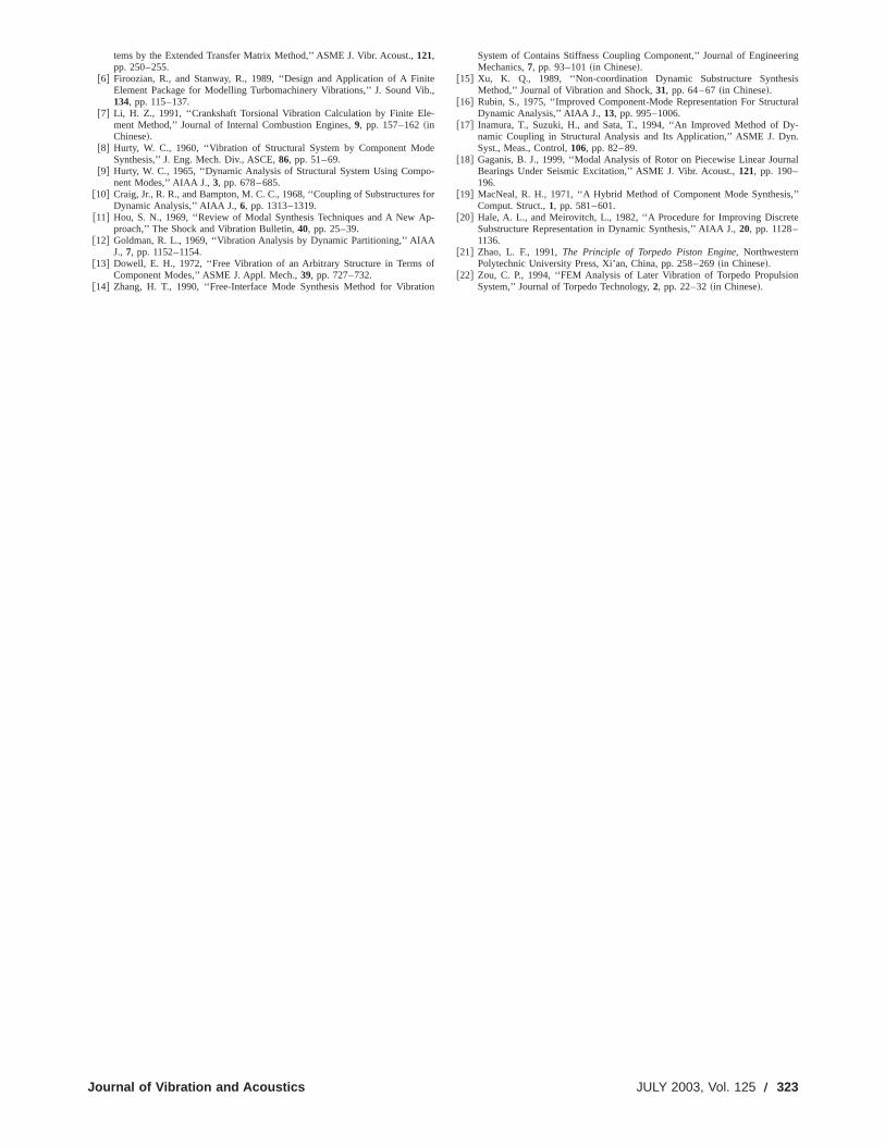
tems by the Extended Transfer Matrix Method,’’ ASME J. Vibr. Acoust.,121,pp. 250–255.

@6# Firoozian, R., and Stanway, R., 1989, ‘‘Design and Application of A FiniteElement Package for Modelling Turbomachinery Vibrations,’’ J. Sound Vib.,134, pp. 115–137.

@7# Li, H. Z., 1991, ‘‘Crankshaft Torsional Vibration Calculation by Finite Ele-ment Method,’’ Journal of Internal Combustion Engines,9, pp. 157–162~inChinese!.

@8# Hurty, W. C., 1960, ‘‘Vibration of Structural System by Component ModeSynthesis,’’ J. Eng. Mech. Div., ASCE,86, pp. 51–69.

@9# Hurty, W. C., 1965, ‘‘Dynamic Analysis of Structural System Using Compo-nent Modes,’’ AIAA J.,3, pp. 678–685.

@10# Craig, Jr., R. R., and Bampton, M. C. C., 1968, ‘‘Coupling of Substructures forDynamic Analysis,’’ AIAA J.,6, pp. 1313–1319.

@11# Hou, S. N., 1969, ‘‘Review of Modal Synthesis Techniques and A New Ap-proach,’’ The Shock and Vibration Bulletin,40, pp. 25–39.

@12# Goldman, R. L., 1969, ‘‘Vibration Analysis by Dynamic Partitioning,’’ AIAAJ., 7, pp. 1152–1154.

@13# Dowell, E. H., 1972, ‘‘Free Vibration of an Arbitrary Structure in Terms ofComponent Modes,’’ ASME J. Appl. Mech.,39, pp. 727–732.

@14# Zhang, H. T., 1990, ‘‘Free-Interface Mode Synthesis Method for Vibration

System of Contains Stiffness Coupling Component,’’ Journal of EngineeringMechanics,7, pp. 93–101~in Chinese!.

@15# Xu, K. Q., 1989, ‘‘Non-coordination Dynamic Substructure SynthesisMethod,’’ Journal of Vibration and Shock,31, pp. 64–67~in Chinese!.

@16# Rubin, S., 1975, ‘‘Improved Component-Mode Representation For StructuralDynamic Analysis,’’ AIAA J.,13, pp. 995–1006.

@17# Inamura, T., Suzuki, H., and Sata, T., 1994, ‘‘An Improved Method of Dy-namic Coupling in Structural Analysis and Its Application,’’ ASME J. Dyn.Syst., Meas., Control,106, pp. 82–89.

@18# Gaganis, B. J., 1999, ‘‘Modal Analysis of Rotor on Piecewise Linear JournalBearings Under Seismic Excitation,’’ ASME J. Vibr. Acoust.,121, pp. 190–196.

@19# MacNeal, R. H., 1971, ‘‘A Hybrid Method of Component Mode Synthesis,’’Comput. Struct.,1, pp. 581–601.

@20# Hale, A. L., and Meirovitch, L., 1982, ‘‘A Procedure for Improving DiscreteSubstructure Representation in Dynamic Synthesis,’’ AIAA J.,20, pp. 1128–1136.

@21# Zhao, L. F., 1991,The Principle of Torpedo Piston Engine, NorthwesternPolytechnic University Press, Xi’an, China, pp. 258–269~in Chinese!.

@22# Zou, C. P., 1994, ‘‘FEM Analysis of Later Vibration of Torpedo PropulsionSystem,’’ Journal of Torpedo Technology,2, pp. 22–32~in Chinese!.


Fusheng Lin

Guang Menge-mail: [email protected]

State Key Lab of Vibration,Shock & Noise,

Shanghai Jiao Tong University,Shanghai 200030, P. R. C.

Study on the Dynamics of a Rotorin a Maneuvering AircraftThis paper shows how the dynamics of a rotor in a maneuvering aircraft changes accord-ing to the operation of the aircraft. The mathematical model of an unbalanced rotorsystem located in the maneuvering aircraft is derived. The dynamic characteristics of therotor running at a constant angular speed or a constant acceleration are studied underthe assumptions that the aircraft maneuvers only in a vertical plane and that the pitchingangle and the flight path inclination of the aircraft are equal. The effects of gravity andunbalance parameter are considered. The results show that the unbalanced response of arotor in an aircraft is obviously influenced by the aircraft’s flying status.@DOI: 10.1115/1.1576422#

1 IntroductionIn the previous literatures on rotor dynamics, the supports of

the rotor are assumed to be static and in the same horizontal orvertical direction@1–2#. This is not practical for rotors located inaircraft because the aircraft operates under various conditions dur-ing maneuvering. Many researchers are focused on studies of onlythe maneuvering flight of aircraft@3–7#, but there is no literatureanalyzed the dynamics of a rotor running in an operating aircraft.This paper attempts to determine the dynamic characteristics of arotor and to simulate, more realistically, the response of such arotor in a maneuvering aircraft.

2 Equations of MotionIn Fig. 1, OXYZis a space-fixed and stationary coordinate sys-

tem, andO1X2Y2Z2 is an aircraft-carried coordinate system par-allel to OXYZ. It is supposed that the pitching angle and the flightpath inclination of the aircraft are equal and defined asa, i.e., theaxis of the rotor shaftO1Z1 is in the same direction as the longi-tudinal axis of the fuselage. It is also assumed thatO1X1Z1 is in

the same vertical plane withOXZ and O1X2Z2 , and the aircraftmoves only in the vertical plane. A Jeffcott rotor model is used.The displacements of the disk center are all measured in a body-fixed and rotatingO1jhz reference frame, wherej andh are inthe principal directions of the cross-section of the shaft andzcoincides with theY1 axis, as shown in Fig. 2. The flexibility ofthe rotor isr. The temporary position of the disk center isO3 . Theposition of the mass center of the disk isC. The angle between theaxesO1h and O1Y1 is b. The coordinateO1jhz rotates withrespect toO1z(O1Z1) with an angular speedb. It is noted thate0

is a reference eccentricity,m is the equivalent mass of the heavydisk mounted at the mid-span of a massless elastic shaft,e is theeccentricity of the disk,u is the angle between the orientation ofthe eccentricity and theh1 axis,k is the stiffness coefficient of theshaft, andc is the external viscous damping coefficient of the shaftand disk.

The dimensionless differential equations of motion of the rotorsystem can be written as follows:

5jd91b9~hd1U cosu!1

2«

Vjd81F 1

V22b8221

2a82~11cos 2b!Gjd12b8hd81S 2«

Vb82

1

2a82 sin 2b Dhd2Ub82 sinu

1F Ge

V2 cosa2Ua82 sin~b1u!Gcost1F2«

V~xd8 cosa2zd8 sina!1xd9 cosa2zd9 sinaGcost50

hd92b9~jd1U sinu!12«

Vhd81F 1

V22b8221

2a82~12cos 2b!Ghd22b8jd82S 2«

Vb81

1

2a82 sin 2b D jd2Ub82 cosu

1 F Ge

V2 cosa2Ua82 sin~b1u!Gsint1F2«

V~xd8 cosa2zd8 sina!1xd9 cosa2zd9 sinaGsint50

(1)

where,jd5j/eo , hd5h/eo , vc5Ak/m, «5c/2mvc , V5v/vc ,

Ge5g/vc2eo , U5e/eo , xd5x/eo , zd5z/eo . « is the dimension-

less viscous damping coefficient,Ge is the gravity parameter,U isthe unbalance parameter, and8 denotes differentiation with respectto dimensionless timet.

If the movement of the aircraft is given, i.e.,x(t) andz(t) are

given, then the anglea can be calculated by

Contributed by the Technical Committee on Vibration and Sound for publicationin the JOURNAL OF VIBRATION AND ACOUSTICS. Manuscript received August 2002;Revised manuscript received March 2003. Associate editor: G. Flowers.

tga5dx

dz5

dx

dt•S dz

dt D21

5x

z5

x8

z85

xd8

zd8,

a5arctgS xd8

zd8D .

Accordingly,a8 can be obtained.The numerical response of the system inO1jhz coordinate can

be obtained by the Runge-Kutta integration method. Response inO1X1Y1Z1 coordinate can also be obtained through a coordinatetransformation.

Equation~1! describes an unbalanced rotor system located in anaircraft moving in the vertical plane. Assuming that the rotatingmotion of the rotor, i.e.,b9 andb8 can be obtained, Eq.~1! can be


simplified and then solved. When the rotor rotates at a constantspeedV, thenb950 andb85V05V. If the rotor accelerates ata constant rate of accelerationCa , then b95Ca.0 and b85V01Cat, whereV0 is the initial angular speed of the rotor.

3 Numerical AnalysisWhen the aircraft flies at a constant rate of acceleration, the

dimensionlessxd08 andzd08 , xd8 andzd8 , andxd9 andzd9 are assumedto be the initial velocity components, the velocity components,and the acceleration components in the directions of theX and theZ axes, respectively. Thenzd85zd08 1zd9t andxd85xd08 1xd9t. If theflight path of an aircraft is a sine curve in the vertical planeOXZand the horizontal component of the aircraft velocity is constant,the motion can be written asxd5xd01G sin(lzd8t). Thereby theacceleration components of the aircraft can be obtained. When therotor rotates at a constant speed, the responses at three differentspeed ratios (V50.8,0.3,1.6) are calculated. When the rotor ro-tates at a constant acceleration, two cases of the initial speed ratio(V050.8,0.3) are investigated.

The numerical responses of some cases are shown from Fig. 3to Fig. 7. In these figures the amplitude refers to the maximumamplitude of the disk center in every revolution and is nondimen-

sionalized as the ratio of the actual amplitude of the disk center tothe reference eccentricitye0 . In each figure, the amplitude isshown in the form of the natural logarithm with base 2.71828 ofthe dimensionless amplituder e5Ajd

21hd2/e0 . The velocity and

the acceleration are assumed to change suddenly at the beginningof the aircraft’s action. In all cases,«50.08. Data was taken for50 revolutions after the response became stable, following this,the status of the aircraft changes.

3.1 Constant Rotor Rotating Speed

3.1.1 Influence of the Aircraft Velocity on Rotor ResponseThe numerical results show that the steady-state amplitudes fordifferent horizontal velocities are the same, which means thatchanging the horizontal velocityzd8 has no influence on the re-sponse amplitude. When the aircraft climbs at a constant velocityand the vertical velocity component is set to different values, theamplitude varies withxd8 . Largerxd8 corresponds to smaller am-plitude. WhenV changes, the difference between the amplitudesin different vertical velocities changes also. The influence of thevertical velocity component of the aircraft whenV50.3 is weakerthan whenV50.8.

3.1.2 Influence of the Aircraft Acceleration on Rotor ResponseWhenV50.8, the amplitude of the disk increases suddenly whenthe aircraft accelerates abruptly in the vertical direction but thehorizontal velocity component remains unchanged. The amplitudedecreases with time until reaching a steady value~Fig. 3!. Thesteady-state amplitude is smaller than the value whenxd950. Theincreasing amount of response amplitude depends on the value ofxd9 when the aircraft accelerates in the vertical direction. Largervalues ofxd9 correspond to larger amplitudes. The difference be-tween the steady-state amplitudes for different values ofxd9 issmall. ChangingGe hardly affects the steady-state amplitudewhen the aircraft is accelerating. However, a larger value of theparameterU will cause larger steady-state amplitude.

WhenV is small, the increase in amplitude is less and the timeneeded to reach steady state is shorter.

3.1.3 Rotor Response When Aircraft Flies in a Sine Curve inthe Vertical Plane OXZ. It is supposed that xd5xd0

1G sin(lzd8t) and the horizontal velocity of the aircraft is unal-tered, i.e.,zd950 andzd85zd08 5constant. In this case,lzd8 denotesthe period of the motion. The maneuvering range in the verticaldirection is reflected byG. The following two cases are calculated.~1! G changes whilel andzd8 are invariant;~2! zd8 changes whileG

Fig. 1 Sketch of the rotor system located in an aircraft and thespace-fixed stationary coordinates

Fig. 2 The reference frame O1jhz and parallel frame O3j1h1z1

Fig. 3 Influence of accelerating abruptly in vertical direction„constant horizontal velocity component … „UÄ1, GeÄ1, V

Ä0.8, zd9Ä0, zd8Äzd08 Ä100, x d08 Ä100…


andl are unaltered. The response when the aircraft moves only inthe horizontal direction andG50 is taken as the basis for com-parison. The aircraft first flies in a horizontal direction at a con-stant velocity. When the free vibration vanishes away and thesteady state amplitude is reached, data of 50 revolutions are taken.Afterwards, the aircraft maneuvers for several periods. The corre-sponding period in dimensionless time is 120032p.

If the aircraft maneuvers periodically, its velocity and accelera-tion will also vary periodically. The amplitude response of thedisk center changes periodically except at the beginning of aircraftaction. In Fig. 4~a! the amplitude decreases suddenly at the verybeginning of the aircraft maneuver. The vibration response is pe-riodic when the second period of aircraft movement begins, andthe period is the same as that of sine curve (50032p). For mostpart of each period~almost 80%! the amplitude is less than thatfor G50, but for some parts the amplitude is larger than that forG50. The amplitude fluctuates acutely when the aircraft starts tomaneuver. Then the fluctuation decreases. The peak amplitudevalue for G5100000 is almost 50% greater than that forG50,and is almost 26% greater than that forG550000 (Ge50.5,U50.5). In Fig. 4~b!, larger values ofzd8 correspond to smalleraircraft maneuvering periods, relatively smaller periods of vibra-tion response and larger peak values. This indicates that quickmaneuvering of the aircraft will cause the vibration response ofthe rotor system to change dramatically, although the maneuverrange in the vertical plane is unchanged.

When V becomes smaller, the increased amplitude due to theaircraft’s maneuver is less and the fluctuation is reduced.

3.2 Constant Angular Acceleration of the Rotor

3.2.1 Influence of the Aircraft Velocity on Rotor Response(b950.00025). If the aircraft is static, the steady state unbal-ance response of the rotor at constant speed acceleration appearsto fluctuate rapidly after the critical rotating speed. Whenxd8.0and is invariable, differentzd8 lead to obviously different responseat the beginning of the rotor acceleration. With the rotor speedincreasing, the difference between responses becomes smaller andthen vanishes. A smaller value of amplitude corresponds to a largexd8 . Whenzd8 remains constant, the response curves for differentxd8 are clearly different at the beginning of acceleration.V0 ap-pears to have no effect on the response.

3.2.2 Influence of the Aircraft Acceleration on Rotor Response(b950.00025). For different aircraft accelerations, the re-sponses of the rotor at low speed range are also different, but theresponses at high speed range may be almost the same~Fig. 5~a!!or very different~Fig. 5~b!! depending on the values ofzd09 andzd9 . Ge has little influence on the response curve, but larger valuesof U correspond to larger amplitude. The responses forV050.3are like those forV050.8.

Fig. 4 Rotor responses when the aircraft flies in a sine curve „VÄ0.8, UÄ0.5, GeÄ0.5, zd9Ä0, lÄ0.00002… „a… Influenceof G „zd8Ä100… „b… Influence of zd8 „GÄ50000…

Fig. 5 Influence of the aircraft acceleration in horizontal and vertical directions on rotor accelerating response „V0

Ä0.8, x d9Ä0, 10, 50, x d8Äzd8Ä100, GeÄ1, UÄ1.0… „a… zd09 Äzd9Ä0 „b… zd09 Äzd9Ä100


3.2.3 Rotor Response When Aircraft Flies in a Sine Curve inVertical Plane OXZ(b950.00025). When the aircraft flies in asine curve andV050.8, the rotor response amplitude at the be-ginning of the rotor acceleration decreases and the response curvefluctuates. The response is not influenced by the parameters of thesine curve when the rotor speed is near or at the critical speed.When the rotor speed is much greater than the critical speed, theresponse curve is significantly influenced by aircraft maneuveringand fluctuates slowly~Fig. 6!. The fluctuation at the beginning ofrotor acceleration and after the critical speed is reduced ifU in-creases orGe decreases.

When the initial rotating speed is small (V050.3), the re-sponses are different for different values ofG ~Fig. 7!. Beforereaching the critical speed, the response fluctuates slowly. IfGÞ0, the response has many peak values equal to the value on theG50 curve, this means that the amplitude of the rotor with con-stant acceleration is less than that of the rotor with lower rotatingspeed and no aircraft maneuver. Aircraft maneuvering has no in-fluence on the response peak amplitude.

4 Conclusions1! The operation of an aircraft affects the dynamics of the rotor

located in it. When the aircraft maneuvers at a constant accelera-tion in the vertical and/or horizontal directions, the amplitude of

the rotor running at a constant speed increases suddenly at thevery beginning of aircraft acceleration and eventually becomesstable, except when the aircraft moves and accelerates only in thehorizontal direction. When the rotor rotates at a constant accelera-tion, the amplitude fluctuates before the critical speed. Differentaircraft acceleration lead to much different rotor responses whenthe rotor runs at a constant rotating speed or at a constant accel-eration.

2! The response of the rotor rotating at a constant speed isclearly influenced by the amplitude and the period of the flightpath when the aircraft moves in a sine curve in the vertical plane.The response curve appears to be periodic except at the beginningof the aircraft action, the period is the same as that of the sinecurve. The gravity parameter affects the response significantly,especially the trend of the response curve. The unbalance param-eter affects only the amplitude value.

3! When the aircraft flies in a sine curve in the vertical plane,the response of the rotor running at a constant acceleration isdifferent from that when the aircraft has no maneuvering, mainlyat the beginning of the acceleration and after the rotor speedpasses through the critical speed. The response curve is obviouslyinfluenced by the gravity parameter when the initial speed is lowin the case of acceleration.

AcknowledgmentThe support from China ‘‘863’’ Project~No. 2002AA412410!

and The Doctor Subjects Research Founding of China University~No. 20020248053! is gratefully acknowledged.

References@1# Lee, A. C., Kang, Y., Tsai, K. L., and Hsiao, K. M., 1992, ‘‘Transient Analysis

of an Asymmetric Rotor-Bearing System during Acceleration,’’ ASME J. Ind.,114~4!, pp. 465–475.

@2# Ganesan, R., and Sankar, T. S., 1993, ‘‘Resonant Oscillations and Stability ofAsymmetric Rotors,’’Proc. of the 14th Biennial ASME Conference on Me-chanical Vibration and Noise, ASME DE, 56, pp. 19–22.

@3# Spence, A. M., and Cele, R., 1995, ‘‘Coupled Rotor Fuselage Dynamics andAero-Elasticity in Turning Flight,’’ J. Am. Helicopter Soc.,40~1!, pp. 47–58.

@4# Cao, Y., 1999, ‘‘Modelling the Unsteady Aerodynamic Forces of a Maneuver-ing Rotor,’’ Aircraft Engineering and Aerospace Technol.,71~5!, pp. 444–450.

@5# Bagai, A., Leishman, J. G., and Park, J., 1999, ‘‘Aerodynamic Analysis of aHelicopter in Steady Maneuvering Flight Using a Free-Vortex Rotor WakeModel,’’ J. Am. Helicopter Soc.,44~2!, pp. 109–120.

@6# Park, J. S., and Leishman, J. G., 1999, ‘‘Investigation of Unsteady Aerody-namics on Rotor Wake Effects in Maneuvering Flight,’’Annual ForumProceedings-American Helicopter Society, 1, pp. 467–480.

@7# Krothapalli, K. R., Prasad, J. V. R., and Peters, D. A., 2001, ‘‘Helicopter RotorDynamic Inflow Modelling for Maneuvering Flight,’’ J. Am. Helicopter Soc.,46~2!, pp. 129–139.

Fig. 6 Rotor accelerating response when the aircraft flies in a sine curve „V0Ä0.8, UÄ0.5, GeÄ1.5, zd9Ä0… „a… Influ-ence of G „zd8Ä100, lÄ0.00002… „b… Influence of zd8 „GÄ100, lzd8Ä0.002…

Fig. 7 Rotor accelerating response when the aircraft flies in asine curve „V0Ä0.3… „UÄ0.5, GeÄ1.5, zd8Ä100, zd9Ä0, lÄ0.00002, GÄ0, 50000, 100000…


Jinhao Qiue-mail: [email protected]

Junji Tani

Taekyu Kwon

Institute of Fluid Science, Tohoku University,Katahira 2-1-1, Aoba-ku, Sendai 980-8577,

Japan

Control of Self-Excited Vibrationof a Rotor System With Active GasBearingsThis paper presents an experimental study on the active control of self-excited vibrationsin a rotor-bearing system supported on a pair of externally pressurized thrust bearings inthe axial direction and on actively controlled journal gas bearings in the radial direction.The active journal gas bearings used are of the tilting-pad type with one traditionalpassive pad and two active pads with embedded piezoelectric actuators. Feedback controlsystems are constructed with gap sensors for measuring the vibration of the rotor, embed-ded piezoelectric actuators, and PID controllers. The experimental results show that theself-excited vibration can be effectively suppressed with the designed feedback controlsystem, if the gains of the PID controllers are properly tuned.@DOI: 10.1115/1.1576423#

1 IntroductionSince gas bearings use gas as a lubricant, they can work in a

wide range of temperatures and have been widely used in turbocompressors and expanders of helium liquefiers@1,2,3#. One ofthe main problems with gas bearings is their intrinsic fluid-relatedhydrodynamic instability as the rotor exceeds twice the naturalfrequency of the rotor rigid body mode. The instability is due tothe interaction between the journal and the gas used as the lubri-cant. The stability of the gas bearings has been greatly improvedwith better designs such as spiral grooves, tilting pads and elasticfoils. In these cases, rotors supported by gas bearings can reachvery high rotational speeds@1,4#. However, self-excited vibrationsin rotor systems supported by gas bearings have always been animportant issue, and a further enhancement in stability is requiredin practical applications.

In some cases, a modification of the configuration or some pa-rameters of the design can prevent gas bearings from undergoingself-excited vibration@5,6#. For example, Ihara@6# designed amovable pivot with an integrated spring, which can adjust thepressing force between the pad and the journal, to increase thedamping effect of the bearing system. The new pivot had theability to suppress the self-excitation of the rotor system, but thefriction between the pads and shaft also prevented the shaft fromstarting rotation when the torque was too small.

Recently, the active control of the self-excited vibration in gasbearings has begun to attract attention, due to the increasing de-mands for high rotation speed and stability@7–11#. Recent ad-vances in sensor and actuator technology and electronics havealso made the active control of gas bearings possible. Many stud-ies on the active control of externally pressurized bearings havealso been reported, but no research has been reported on the activecontrol of tilting-pad journal gas bearings, probably due to theircomplicated configuration and vibration mechanism.

In this study, an active pad, supported by a pivot with an em-bedded piezoelectric actuator, is proposed for active tilting-padjournal gas bearings and used in the active control of the self-excited vibration of a rotor-bearing system. The rotor is supportedon a pair of externally-pressurized thrust bearings~EPTB! in theaxial direction, and on active journal gas bearings in the radialdirection. The radial position of the active pads in the journalbearing can be actively adjusted by applying a voltage to theembedded piezoelectric actuators. Experiments were performedon the active control of the self-excited vibration in the rotor-

bearing system using the control force generated by the two activejournal gas bearings. The effectiveness of the active pads wasconfirmed by experimental results.

2 Configuration and Vibration Characteristics of theRotor-Bearing System

Figure 1 shows the configuration of the rotor-bearing system,originally designed for use in a high-expansion-ratio turbo ex-pander of a helium liquefier, shown in Fig. 2. The rotor consists ofa shaft, a turbine impeller at one end of the shaft for the genera-tion of the driving moment, and a blower impeller for braking atthe other end. The rotor of the expander is supported by twotilting-pad journal gas bearings in the radial direction and a pair ofexternally pressurized thrust gas bearings in the axial direction.The rotor can reach a maximum speed of 35,000 rpm at a drivingair pressure of 0.5 MPa on the turbine impeller.

The rotor is installed vertically and its weight is supported bythe thrust bearings. Since the load in the radial direction is verysmall, tilting-pad journal gas bearings are used. The total length ofthe rotor is 181.35 mm and the two tilting bearings are located at23.54 mm above and 26.46 mm below the center of mass of therotor, as shown in Fig. 2~a!. The cross-sectional view of thetilting-pad journal gas bearing used in the rotor-bearing system isshown in Fig. 2~b! and Fig. 3. There are three tilting pads in eachbearing. The width of a pad is 15.4 mm and its spanning anglebis 110 deg. The nominal clearanceCr is 20mm and the preload ofthe pads is 0.5. The parameters of the rotor-bearing system aresummarized in Table 1. The dynamic characteristics of the tilting-pad gas bearings are discussed in@4#.

The externally-pressurized thrust bearing was used to supportthe high thrust load resulting from the impeller. The thrust bear-ings are a pair of the inherently compensated annular bearingsshown in Fig. 4. Their outer and inner diameters are 32 mm and16.4 mm, respectively. There are 18 nozzles uniformly distributedin a circle of r a522.4 mm in each thrust bearing. The diametersof the upper and lower bearings are 0.3 mm and 0.6 mm, respec-tively. The parameters of the thrust gas bearings are summarizedin Table 2. The design and dynamic characteristics of theexternally-pressurized thrust bearings are discussed in@1#.

The vibration of the rotor is measured using eddy-current gapsensors with a sensitivity of 0.5mm. The four gap sensors aredivided into two groups and fixed at two planes at 10.84 mmabove and 14.16 mm below the center of mass of the rotor. Thetwo gap sensors in the same plane are mounted 90 deg apart andmeasure the lateral displacement of the shaft in that plain, asshown in Fig. 3. The positions of the sensors are labeled as LR,

Contributed by the Technical Committee on Vibration and Sound for publicationin the JOURNAL OF VIBRATION AND ACOUSTICS. Manuscript received March 2002;Revised March 2003. Associate Editor: G. Flowers.


LL, UR and UL. The LR and LL sensors are installed in the lowerplane and the UR and UL sensors are installed in upper plane.Moreover, the LL and UL sensors measure the displacement of theshaft in they direction, and the LR and UR sensors measure thedisplacement in thex direction of the right-handed coordinate sys-tems shown in Figs. 1 and 3.

The characteristics of the rotor vibration are measured using thefollowing procedure. Firstly, a 40 V DC voltage is applied to allfour piezoelectric actuators as a bias voltage in the vibration con-trol of the rotor system. Secondly, the thrust bearing is activatedby supplying pressurized air. Thirdly, the valves of the gas sup-plies for the driving impeller and the braking impeller are turnedon to start the rotation of the shaft. The rotation speed of the shaft,determined by the relative pressure of the air supplied to the driv-ing impeller and the braking impeller, is raised to 30,000 rpm byincreasing the flow rate of the air to the driving impeller and thenreduced to 0 rpm again by decreasing the flow rate. The vibrationof the shaft is measured when the speed of the rotor reduces from30,000 rpm to 0 rpm.

Figure 5 shows the waterfall plot of the vibration characteristicsin the y direction measured by the LL sensor. It can be seen thatboth the synchronous vibration with the frequency equal to therotation speed, and the asychronous vibration~self-excited vibra-tion!, are induced in the rotor system. The sychronous vibrationreaches the maximum amplitude at 11,600 rpm, which equals thenatural frequency of the first rigid mode of the rotor. The fre-quency of the self-excited vibration is about 57 Hz, regarless ofthe rotational speed, but its amplitude also reaches the maximumvalue at around 11,600 rpm. The fluid-related instability in boththe journal bearings and the thrust bearings can induce the self-excited vibration. A dynamic coupling between the journal bear-ings and the thrust bearings may also occur in the rotor-bearingsystem. The objective of this study is to control the self-excitedvibration of the rotor-bearing system.

3 Active Gas BearingsIn order to control the vibration of the shaft, piezoelectric ac-

tuators were embedded in two of the three pivots in each bearing,as shown in Fig. 3. The piezoelectric actuators are 535310 mm in size and can generate 6.1mm of displacement at 200V input voltage. The piezoelectric actuators, which have a widefrequency bandwidth and can generate a large force output, aresuitable for this kind of application. The positions of the fouractuators are also labeled as LR, LL, UR and UL. The LL and ULactuators are embedded in the pivots on they-z plane and the LRand UR actuators are embedded in the pivots on the plane at 30degrees clockwise from thex-y plane.

When the shaft rotates, a pressurized gas film is formed be-tween the shaft and each pad due to the viscosity of the gas. The

rotor is supported by the pressure of the gas films in the radialdirection. The pressure distribution of the gas film, and thereforethe resultant force due to pressure, are dependent upon the clear-ance distribution between the shaft and pads. The resultant forcecan be actively controlled by changing the radial position of thepivot. Therefore, the vibration of the shaft can be actively sup-pressed when an appropriate voltage is applied to the piezoelectricactuators.

In order to investigate the static characteristics of the PZT ac-tuators in the rotor-bearing system, the bias displacements of therotor are measured at the four sensors when a DC voltage wasapplied to the UR actuator during operation. The bias displace-ments are the DC components of the rotor displacement, that is,the displacements of the whirling center of the rotor. Figure 6shows the results measured at 11,600 rpm. As the voltage in-creased from 0 V to 150 V, the displacements of the shaft mea-sured by the LR and UR gap sensors decreased from 0mm to24.3 mm, while the displacements of the shaft at the LL and ULsensors increased from 0mm to 2.2 mm at a rotation speed of11,600 rpm. This means that, due to the static displacement gen-erated by the PZT actuator in the UR pad, the rotor moves awayfrom the LR and UR sensors but closer to the LL and UL sensors.

4 Control System and Experimental SetupFigure 7 shows the configuration of the experimental setup of

the rotor system and the feedback control system used. Since it isdifficult to derive a mathematical model of the dynamical system,a PID control method that does not require a mathematical modelof the control object is used in this study. It is also assumed thatthe interaction between the actuators is negligible and that eachactuator can be controlled independently. The input-output rela-tionship of the controller for each actuator is defined by the fol-lowing equation:

U~s!

Y~s!5Kp1Kds1

Ki

s5KpS 11Tds1

1

TisD (1)

whereY(s) is the feedback signal~in volts!, U(s) is the controlinput ~the voltage applied to the actuators in volts!, andKp , KdandKi are the proportional, derivative and integral gains, respec-tively. Moreover,Ti5Kp /Ki andTd5Kd /Kp are the integral andderivative constants.

Different gains were selected for different actuators in the ex-periment. For the actuator installed in the same direction as thesensor, the output of the sensor was used directly as the feedbacksignal Y(s). For the actuators at the LR and UR positions, thefeedback signalY(s) was estimated from the output of the twosensors at the nearest measuring plane.

Figure 8 shows a block diagram of the active control system.The analog signals from the sensors are sampled at a frequency of

Fig. 1 Configuration of the rotor-bearing system


Fig. 2 Configuration of the high-expansion-ratio expander „a… Longitudinalcross-section „b… Transverse cross-section


10 kHz through an A/D converter and then transmitted to a DSP.The designed controller was implemented digitally in the DSP,and the control input calculated on the basis of the sensor signals.The calculated control input was added to a bias voltage, ampli-fied and then applied to the actuators. The bias voltage was super-posed on the input voltage calculated from Eq.~1! in order toincrease the maximum output displacement of the actuators. Thegain of the power amplifier is 20 and the bias voltage after am-plification is 40 V. The gain of the sensor and the power amplifierare not included in the transfer function in Eq.~1!.

5 Results and DiscussionsDue to the influence of the pressurized air supplied to the driv-

ing impeller, the actuators at LL and LR were less effective in thecontrol of the self-excited vibration than the other two actuators.Therefore, the gains of these two actuators were fixed atKd50.01, Ki50.001 andKp550, while the gains of the other twoactuators at UL and UR were varied to investigate their influence.Moreover, the integral gain of the two actuators at UL and URwas also set to 0.001, since it has little influence on the controleffect. Control experiments were performed for different combi-nations ofKp and Kd for the actuators at UL and UR. Figure 9shows the shaft frequency response measured by the sensors atUR and LR for a rotation speed of 10,000 rpm with gainsKp andKd for the actuators at UL and UR set to 10 and 0.02, respectively.The asynchronous vibration~about 57 Hz! was significantly re-

duced. However, the synchronous vibration remained almost un-changed. The small peak at 50 Hz is due to the electromagneticnoise of the power supplies.

Figure 10 show the rotor frequency response measured by thefour sensors at 11,600 rpm.Kd was set to 0.01, and the propor-tional gainsKp of the UL and UR actuators were set to the opti-

Fig. 3 Configuration of the tilting-pad journal gas bearings

Table 1 Parameters of the rotor-bearing system

Shaft length,l 181.35 mm l 1 23.54 mmShaft mass,m 0.28 kg l 2 26.46 mmShaft radius,R 8 mm l 3 10.84 mmBearing width,L 15.4 mm l 4 14.16 mmLength of pad,b 110° l 5 90.25 mmClearance,Cr 20 mm l 6 91.1 mmPivot positionbp /b 0.65 l 7 38.74 mmDimensionless preload 0.5 l 8 6 mm

Fig. 4 Configuration of the externally-pressurized thrust gasbearings „a… Distribution of nozzles „b… Upper and lowerclearances

Table 2 Parameters of the thrust bearing

Outer diameter,r 1 32 mmInner diameter,r 0 16.4 mmDiameter of nozzle position circle,r a 22.6 mmNumber of nozzles,n 18Diameter of nozzles in the lower bearing,r s1 0.6 mmDiameter of nozzles in the upper bearing,r s2 0.3 mmUnloaded clearance of the lower bearinghn1 23.4mmUnloaded clearance of the upper bearinghn2 16.6mmNondimensional axial displacementDhn /(hn11hn2) ,0.22

Fig. 5 Waterfall chart of the frequency response of the rotor atthe LL gap sensor „experimental result …


mal values of 150 and 100, respectively. Since the rotor speedequals the resonant frequency of the rotor-bearing system, theamplitude of the asynchronous vibration increases significantly atthe uncontrolled state. However, the asynchronous vibration isalmost completely suppressed after control. Despite this, little ef-fect could be observed on the synchronous vibration. The othercomponents of the asynchronous vibration with frequencies of 25Hz, 79 Hz and 132 Hz were also suppressed.

The influence of the feedback gain on the control results wasfurther investigated. Fig. 11 shows the control results when theproportional gains of the actuators at UL and UR were set to 200,while the rotor speed and the other gains were kept the same asthose in the former case. The asynchronous vibration at a fre-quency of 57 Hz was almost completely suppressed. However, asecond asynchronous vibration of 93 Hz was excited.

Figure 12 shows the rotor frequency response measured by theUR sensor when theKp of the actuators at UL and UR was set to10, andKd was set to 0.2 for Case~a! and 0.01 for Case~b!. InCase~b!, the asynchronous vibration of 57 Hz was satisfactorilysuppressed, though a low peak remained due to the small propor-tional gain. However in Case~a!, another asynchronous vibrationof 67 Hz was significantly excited. Moreover, the gains used inCase~b! are the same as those in Fig. 9, except thatKd decreasedfrom 0.02 to 0.01. This means that the same gains can yield goodcontrol performance for a range of rotor speeds. The equivalentstiffness and damping coefficients of the closed-loop system cor-responding to the proportional and differential gains cannot beestimated quantitatively since the mathematical model of the con-trol plant is unknown. However, their variation can be observedfrom the position and shape of the peak corresponding to theasynchronous vibration in the power spectra shown in Fig. 9–12.The decrease in the stiffness coefficients moves the peak of theasynchronous vibration to the left side~Fig. 9!, while the peakbecomes sharper as the damping coefficient decreases~Fig. 10!.

Fig. 6 Bias displacement of the shaft versus DC voltage ap-plied to the UR actuator

Fig. 7 Schematic diagram of the active control system

Fig. 8 Block diagram of the control system

Fig. 9 Power spectra of the shaft at the LR sensor position„Rotation speed: 10,000 rpm, PID gain: K p of UL act. Ä10, K p ofUR act.Ä10…


Fig. 11 Power spectra of the shaft at the UL sensor position„Rotation speed: 11,600 rpm, PID gain: K p of UL act. Ä200, K p ofUR act.Ä200…

Fig. 12 Power spectra of the shaft at the UR sensor position„Rotation speed: 11,600 rpm, „a… PID control: K d of UL Act.Ä0.2, K p of UL act. Ä10, „b… K d of UR act. Ä0.01, K p of UR act.Ä10…

Fig. 10 Power spectra of the shaft at different sensor positions „Rotation speed: 11,600 rpm, PID gain: K p of UL act. Ä150, K pof UR act. Ä100… „a… UL sensor position „b… LL sensor position „c… UR sensor position „d… LR sensor position


6 ConclusionsA novel tilting-pad journal gas bearing system with active pads

was studied for the control of self-excited vibration in a rotorbearing system. Each active pad contains an embedded piezoelec-tric actuator, used to adjust the clearance between the shaft andpads. The novel gas bearings were used in the rotor system of ahigh-expansion-ratio turbo expander for helium liquefier, and afeedback control system was constructed with four gap sensors,embedded actuators and PID controllers. It was confirmed by ex-periment that the self-excited vibration in the rotor system couldbe effectively suppressed with the feedback control if the gains ofthe controllers were appropriately chosen.

It was also found that little control was achieved for the syn-chronous vibration of the rotor system using the present configu-ration. The active control of synchronous vibration will be thesubject of future work.

AcknowledgmentThe authors thank Dr. Yanagi, and Mr. Tsugawa of Mayekawa

Mfg. Co. Ltd., MYCOM Advanced Technology Laboratory,Ibaraki, Japan, for their effort and cooperation in the design andmanufacturing of the rotor-bearing system.

References@1# Ino, N., Machida, A., Tsugawa, K., and Hashimoto, H., 1991, ‘‘Development

of Externally Pressurized Thrust Bearing for High-Expansion-Ratio HeliumExpander, Trans. Jpn. Soc. Mech. Eng., Ser. C,~in Japanese! 58~550!, pp.1885–1891.

@2# Togo, T., 2000,Investigation Report on the Research of Gas Bearings, Japa-nese Society of Tribologists.

@3# Andres, L. S., 1996, ‘‘Turbulent Flow, Flexure-Pivot Hybrid Bearings forCryogenic Applications,’’ ASME J. Tribol.,118, pp. 190–200.

@4# Qiu, J., Takagi, T., Tani, J., Machida, A., Tsugawa, K., Yanagi, H., and Ino, N.,1993, ‘‘Dynamic Characteristics of a Tilting-pad Bearing System for HighExpansion-Ratio Expander,’’ Adv. Cryog. Eng.,39, pp. 909–914.

@5# Bently, D. E., and Muszynska, A., 1989, ‘‘Anti-Swirl Arrangements PreventRotor/Seal Instability,’’ Stress, Reliab. Des.111~2!, pp. 156–162.

@6# Ihara, K., 1987, ‘‘Gas Expander for Lower Temperature,’’ Journal of TurbineMachinery~in Japanese!, 15~11!, pp. 57–62.

@7# Palazzolo, A. B., Lin, R. R., Alexander, R. M., Kascak, A. F., and Montague,J., 1989, ‘‘Piezoelectric Pushers for Active Vibration Control of Rotating Ma-chinery,’’ ASME J. of Vibration, Acoustics, Stress, Reliab. Des.111, pp. 298–305.

@8# Palazzolo, A. B., Jagannathan, S., Kascak, A. F., Montague, G. T., and Kiraly,L. J., 1993, ‘‘Hybrid Active Vibration Control of Rotorbearing Systems UsingPiezoelectric Actuators,’’ J. Vibr. Acoust.,135, pp. 111–119.

@9# Horikawa, O., and Shimokohbe, A., 1990, ‘‘An Active Air Bearing,’’ JSME,Int. Journal,33~1!, pp. 55–60.

@10# Muszynska, A., Franklin, W. D., and Bently, D. E., 1988, ‘‘Rotor Active ‘Anti-Swirl’ Control,’’ Stress, Reliab. Des.110~2!, pp. 143–150.

@11# Sun, L., Krodkiewski, J. M., and Cen, Y., 1998, ‘‘Self-Tuning Adaptive Con-trol of Forced Vibration in Rotor Systems using an Active Journal Bearing,’’ J.Sound Vib.,213~1!, pp. 1–14.


J. A. WickertFellow ASME,

Department of Mechanical Engineering,Carnegie Mellon University,

Pittsburgh, PA 15213

Vibration of Flex Circuits in HardDisk DrivesA flex circuit connects the stationary electronic components in a hard disk drive to therotating arm that carries the read/write heads and positions them above data tracks onthe disk. Flex circuits are conventionally formed as a laminate of polyimide substrate,adhesive, and copper conductors. Deformation of a flex circuit is discussed in the contextof the following stages: the initial unstressed shape, configurations in which stresses setand relax in response to elevated temperature, equilibrium, and small amplitude vibra-tion. The model involves displacements of the flex circuit in the directions tangent andnormal to the local equilibrium shape, and those motions couple with the arm’s dynamics.Nonlinearity associated with finite curvature, partial elastic springback, and the arm’sgeometry and inertia properties are incorporated within the vibration model to predictsystem-level natural frequencies, mode shapes, and coupling factors between the circuitand the arm. Laboratory measurements using noncontact laser interferometry validate themodel with respect to the circuit’s shape, stiffness, restoring moment, and natural frequen-cies. The primary degrees of freedom for optimizing flex circuit design are the thicknessesof the individual layers within the circuit, free length, and the locations and slopes of thecircuit’s attachment points to the arm and electronics block. The model’s predictions andtrends developed from a case study in free length are discussed with a view towardreducing coupling between the circuit and arm in certain vibration modes.@DOI: 10.1115/1.1547661#

1 IntroductionThe storage density of hard disk drives, as measured by the

number of data bits captured within a unit area, has grown at ahistorical rate of about 60% per year, and that rate has acceleratedrecently to more than 100% per year. In a similar vein, the costassociated with storing a megabyte of data has fallen by over fourorders of magnitude during the past two decades. With the physi-cal limit for the density of magnetic disk recording now appearingon the horizon, higher-precision requirements are being placed onthe vibration of each structural and actuation component.

By way of background and motivation, the construction of ahard disk drive is shown in the photograph of Fig. 1. Data isstored as magnetic transitions on the thin media layer that coatsthe glass disks. The arm pivots about a fixed bearing, and it isdriven by a voice coil that swings between two permanent mag-nets. The read/write heads are located at the tip of the arm aboveeach disk surface, but they are not discernible in Fig. 1 because oftheir small size. The particular drive shown in the figure has atotal of ten read/write heads.

The voice coil and its companion servo system slew the headsto a desired cylinder of data, and follow it in the presence of diskrunout, vibration, windage, and other disturbances. Electricalleads are routed to each read/write head to carry the recording andreadback signals, and other larger leads power the voice coil. Eachhead and coil wire is integrated within a flat and flexible circuitthat conveys all of the electrical signals between the~rotating! armand the~stationary! electronics on the drive’s body. This overallconstruction is shown schematically in Fig. 2. In a typical embodi-ment, the flex circuit is a polyimide film laminate having rolledannealed copper wires in its conductor layer. Flex circuits replaceconventional multi-lead wiring and combine electrical functional-ity with mechanical flexibility, which in turn can potentially intro-duce unwanted vibration. Quite aside from hard disk drives, othertypes of flex circuits are used in avionics packages, gyroscopes,hearing aids, and cardiac pacemakers.

The mechanical behavior and vibration of a hard drive’s disks,motor, spindle, bearings, voice coil, and other elements have beenthe subject of substantial engineering development effort since thefirst introduction of a hard disk drive in 1956. As drives havebecome more sophisticated, sources of vibration that had previ-ously been within tolerance limits have become the focus of fur-ther improvement efforts. In particular, the vibration of flex cir-cuits and their coupling with motion of the read/write heads arenow factors in high density recording applications. No longerviewed as a lightweight appendix to the arm and voice coil, theflex circuit has dynamics that couple through the arm and producetrack positioning errors.

Reducing flex circuit vibration in certain modes is a potentialstrategy for improving transient settling response after a seek op-eration to a new data track. From the modeling perspective, anobjective of this investigation is to better understand the flex cir-cuit’s equilibrium shape involving finite deformation and partialelastic springback, and the character of its small amplitude vibra-tion about equilibrium. Of particular interest are the flex circuit’sstatic shape at a specified arm rotation angle, natural frequencies,and coupling to the arm and read/write heads in each mode. Inwhat follows, the roles played by such parameters as the circuit’slaminated structure, finite curvature, free length, and boundaryconditions at the arm and electronics block are explored.

2 Material Characteristics and Loading SequenceIn Fig. 3, the two micrographs of a flex circuit’s cross-section

describe the internal morphology and dimensions of the severalmaterial layers. In optical diagnostics, a segment of the flex circuitwas embedded in epoxy, diced, and polished smooth. A thin layerof gold was then sputtered onto the surface of the cross-section toenhance imaging. The particular circuit of Fig. 3 is formed as asymmetric sandwich laminate of twohp531mm thick polyimidelayers on either side of flat copper electrical leads. Kapton® isoften used as the substrate material, and it is chosen on the basisof electrical, mechanical, and thermal properties. In Fig. 3~a!, amatrix of epoxy bonds the polyimide layers to the conductors, andthe thickness of the intervening adhesive isha513mm. The cir-cuit comprises twenty conductors having commonhc526mm

Contributed by the Technical Committee on Vibration and Sound for publicationin the JOURNAL OF VIBRATION AND ACOUSTICS. Manuscript received May 2002;revised October 2002. Associate Editor: Chin An Tan.


thickness, and one of four different widths depending on the typeof electrical signal being carried. Somed567% of the flex cir-cuit’s b511.15 mm width is associated with the conductors, andthe remaining fraction of space between the conductors remainsinsulated by adhesive. Figure 3~b! depicts a second portion of thesame flex circuit, and its image is spaced width-wise relative toFig. 3~a!. Three adjacent conductors, slight variation in the adhe-sive thickness, and indentation of the conductor into the lowersubstrate are visible features. The cumulative thickness ish5hc12(hp1ha)5114mm, and the flex circuit has linear density2.38 g/m in the direction along its free lengthL.

Vibration of the flex circuit depends in part on its equilibriumcurvature and internal loads, which are distinguished from their

counterparts in the circuit’s natural state where no reactions areapplied through attachment to the arm and electronics block. Fur-ther, the flex circuit’s stresses, particularly in the adhesive layer,are known to partially relax with time and temperature. Deforma-tion from the initial free shape, through finite motion to equilib-rium, and ultimately to small amplitude vibration are broken downin the following sequence of loading states:Initial S (0) The flex circuit is specified to be initially unstressedand straight. Imperfections that are present as a result of the cir-cuit’s production or the drive’s final assembly could be incorpo-rated at this stage by specifying a functional form of curvaturek(0)(s), wheresP(0,L) denotes arc length, but such effects arenot considered at this first level of approximation.Set S(1) Referring to Fig. 2, the flex circuit is bent fromS(0) andattached to the arm and electronics block. Elements within it aresubjected to tensionT(s), shear forceN(s), and bending momentM (s). During the process toS(1), the circuit undergoes finite

Fig. 1 Photograph depicting certain mechanical components within a harddisk drive used for computer data storage

Fig. 2 Schematic of the equilibrium and vibration model forthe arm and flex circuit mechanism

Fig. 3 „a… Brightfield and „b… differential interference contrastmicrographs of flex circuit cross-sections. The images depictthe construction morphology and the thicknesses of the poly-imide, conductor, and adhesive layers.


deformation to the new shape of curvaturek(1). The coordinates(xL ,yL) of the contact point and the angleuL of approach at theelectronics block are specified. Rotationa of the arm is an inde-pendent variable inS(1), and together with the geometric param-etersb, g, and r defined in Fig. 2, its value sets the circuit’sconditions

x~0!5r cos~a2b! y~0!5r sin~a2b! (1)

u~0!5a2g (2)

at its endpoints5L. In S(1), the arm is held by an external agentat an angle that could correspond to the disk’s inner~ID! or outer~OD! diameters, or the load-unload~LU! support where the arm isparked when the drive is not in use.Springback S(2) During both its production and day-to-day usage,the flex circuit is exposed to elevated temperature. Certain fabri-cation stages take place at 80°C; an assembly-level wash/drycycle occurs at 85°C; and the internal environment of a perfor-mance drive can reach 50–60°C. By comparison, the glass tran-sition temperature of an adhesive commonly used within flex cir-cuits lies in the range 50–95°C. In the springback stage, while theflex circuit remains attached to the arm and electronics block inS(1), stresses are allowed to partially relax and the circuit assumesthe new natural stateS(2). To characterize this process, thermalcycling experiments were conducted with the arm locked at thedisk’s inner diameter (a ID564 deg) and the assembly held at45°C for one hour. After having cooled to ambient temperature,the arm and flex circuit assumed nearly that point as the newequilibrium configuration. The arm was then pivoted to the disk’souter diameter (aOD532 deg), thermally cycled, and observed toassume a nearby position in equilibrium. During those processes,however, the stresses within the flex circuit were only partiallyreduced. Indeed, when the circuit was cut free and released, itassumed a new natural state having shape and curvature some-what betweenk(0) andk(1). The empirical factorp is introduced toquantify the amount of elastic springback that occurs when theflex circuit is unloaded, and the curvature inS(2) is definedk(2)

5(12p)k(1). Whenp51, the circuit behaves elastically, is unaf-fected by exposure to elevated temperature, and returns to its ini-tial straight shape when unloaded fromS(1). On the other hand,whenp50, the flex circuit assumesS(1) as the new natural state.In practice, the actual loading process andk(2) lie between thesetwo extremes, and they change in a time-, temperature-, andhistory-dependent manner as the arm continuously slews betweenthe disk’s ID and OD. In the baseline parameters of Table 1, thevaluep50.55 was determined by experience in thermally cyclingseveral disk drives and examining the circuits when they were cutand released from the arm and electronics block. The flex circuitswere photographed, and their natural shapes were compared tothose predicted by the equilibrium model described below at vari-ous levels of springback. Parameterp was then adjusted by cut-and-try until the predicted and measured natural shapes wereagreeably close.Equilibrium S (3) From the natural configurationS(2), the flexcircuit is imagined to be re-attached to the arm and electronicsblock. With no external torqueMo about the pivot point beingapplied by the voice coil, the arm rotates to equilibrium in re-sponse to the combined influence of the tension, shear force, andbending moment ats50. At this stage, the arm’s equilibriumangle and the circuit’s curvature are denoted bya* and k*5k(3), respectively.Deformed S(4) In this loading stage, the flex circuit is elasticallydeformed about equilibrium, corresponding to static slew at a cer-tain angle, to small amplitude vibration of the flex circuit aboutequilibrium, or to finite amplitude vibration. The tension, shearforce, and bending moment are each incremented relative to theirequilibrium values. Motion of the flex circuit is resolved into the

directions tangent and normal to the local equilibrium, and thosedisplacements are denoted byu(s,t) andv(s,t), respectively.

3 Equilibrium Shape, Loads, and Stresses

The flex circuit’s shape inS(3) is defined parametrically by thecoordinates (x(s),y(s)). With the nomenclature (d)85d/ds,equilibrium in the local tangential and normal directions is gov-erned by the force and moment balances@1#

T85Nk, N852Tk, k852N/EI1k~2!8 (3)

in which the constitutive relationM5EI(k2k(2)) has been em-bedded. The circuit’s bending stiffness is given by

EI51

12Echc

3db11

12Eahc

3~12d!b12EaS 1

12bha

311

4bha~hc

1ha!2D12EpS 1

12bhp

311

4bhp~hc1hp12ha!2D (4)

where values for the elastic constants of the conductorEc , poly-imide Ep , and adhesiveEa are listed in Table 1. While Eq.~4! isspecific to the cross-sectional construction of Fig. 3, the treatmentcan be adapted for other geometries.

On the basis of measured layer thicknesses and published elas-tic constants@2# in Table 1, the circuit’s composite bending stiff-ness isEI54.7831026 N•m2. The conductor layer contributes26% to the stiffness, the polyimide layer 71%, and the adhesivelayer only 3%. This value ofEI was validated by both static bend-ing and natural frequency measurements conducted with a circuitsegment that was embedded as a cantilever in an epoxy casting. Inthe static test, the segment was mounted on a micrometer transla-tion stage, and under specified displacement, the force applied toit’s tip was measured. The signal from a planar beam sensor~Fu-tek FR-1020! was conditioned and amplified to provide a cali-brated and linear force response for loads up to 295 mN. The

Table 1 Baseline parameters for the arm and flex circuit’sequilibrium and vibration models

Flex Circuit

Width, b 11.1 mmThickness

Polyimide layer,hp 31 mmAdhesive layer,ha 13 mmConductor layer,hc 26 mmCumulative,h 114 mm

Conductor fraction,d 67%Free length,L 31 mmComposite linear density,rA 2.38 g/mModulus

Polyimide,Ep 2.75 GPaAdhesive,Ea 1.03 GPaConductor,Ec 115 GPa

Springback ratio,p 0.55Composite bending stiffness,EI 4.783(1026) N•m2

Composite axial stiffness,EA 2.453(104) N

Arm

Attachment radius,r 10.6 mmRead/write head radius,R 43.8 mmAttachment angle,b 95°Offset angle,g 8°Angles

Load-unload,aLU 23°Disk OD, aOD 32°Disk ID, a ID 64°

Inertia,m 17.2 gRadius of gyration,k 11.9 mm

Electronics Block

Coordinates, (xL ,yL) ~24, 211! mmTangency angle,uL 290°


stiffness recorded on this basis was 4.6031026 N•m2. In the sec-ond validation test, the value 4.9131026 N•m2 was determinedby measuring the segment’s two lowest natural frequencies andmatching them to the values expected for a cantilever. In the cal-culations described below, the stiffness value determined from Eq.~4! was used.

The circuit’s equilibrium curvature is determined by integratingEqs.~3!, and its shape is found subsequently from the kinematicrelations

x85cosu, y85sinu, u85k~s! (5)

subject to position and slope conditions ats50 and L. Whilesome rotation between the circuit and arm does occur locally ats50, that effect is neglected in this first approximation, recogniz-ing that the resulting model may overestimate the circuit’s actualboundary stiffness.

Solutions to Eqs.~3! and ~5! are found through a shootingmethod in which the boundary value problem inx, y, and u isconverted to an initial value problem, and then solved iteratively.Estimates for~initially unknown! N(0), T(0), andk(0) are as-signed, and the system of differential equations is integrated nu-merically. The valuesx(L), y(L), and u(L) which result fromthat calculation do not, in general, satisfy the endpoint constraints.In iteration, N(0), T(0), andk(0) are then adjusted through anonlinear minimization scheme until each kinematic condition issatisfied within desired tolerance.

On the basis of the parameters in Table 1, Fig. 4 depicts simu-lated and measured shapes of the flex circuit in its natural (S(2))and equilibrium (S(3)) states. The data points shown in the figurerepresent coordinate locations as extracted from photographs ofthe circuit in the two configurations. Curvature in the natural statewas set with the arm held at the disk’s OD and the springbackconstant beingp50.55. At the equilibrium anglea* 526.4 deg,the tension, shear force, and bending moment applied by the flexcircuit to the arm produce no resultant torque about the pivotbearing. Their variations in response to first-order changes ina,however, are captured by stiffness 10.2 mN•mm/deg.

The equilibrium tension and shear force distributions along thecircuit are shown in Fig. 5. The circuit is compressed over itsentire length with the minimum, mean, and maximum loadingvalues forT being 255, 233, and214 mN, respectively. Thezero crossing in shear occurs at a distance approximately 64%

along the circuit’s length from the arm. While the average strainover the cross-section is onlyT/EA'21.331026 with

EA5Echcbd12Eahab1Eahcb~12d!12Ephpb (6)

the peak bending strainhcuk* 2k(2)u/2 within the conductor layeris 0.12%. For other free lengths, arm positions, or endpoint loca-tions, local yielding could occur within the ductile conductor.

As the arm slews about equilibrium, the flex circuit bends fur-ther to S(4) as shown in Fig. 6. The voice coil applies the staticbias torque

Mo5T~0!r sin~b2g!1N~0!r cos~b2g!1M ~0! (7)

which increases in Fig. 7 from zero at equilibrium to the maxi-mum value 0.35 N•mm at the disk’s ID. Multiple measurementsof the torque were made for one disk drive at four different slewangles, and those results are also shown in Fig. 7. The indicatedvariation ofMo is representative of such measurements and cap-tures hysteresis in the circuit, and friction in the pivot bearing and

Fig. 4 Predicted „ … and measured shapes of the flex circuitin equilibrium with attachment to the arm and electronicsblock, and in its natural state. The shapes extracted from pho-tographs of the circuit in the two states are denoted by the „s…

and „d… data points, respectively.

Fig. 5 Equilibrium tension and shear force along the circuit’sarc length

Fig. 6 Variation of the flex circuit’s static shape for arm posi-tions which range between the disk’s outer and inner diam-eters. For each arm position, the locations of the circuit’s end-points are denoted by „s….


supports. The trend in Fig. 7 is agreeably linear over the operatingrange, although the circuit’s stiffnessdMo /da does decrease inthe disk’s mid-diameter range, and grow again for slew anglesnear the ID.

Figure 8 depicts the manner in which the flex circuit’s equilib-rium shape changes as a function of its free length. Results areshown for simulations in whichL varies between 70% and 130%of its nominal value. With the other parameters of Table 1 remain-ing fixed, the corresponding changes to the arm’s equilibriumangle and the circuit’s static stiffness are listed in Table 2.

4 Natural Frequencies, Vibration Modes, and Cou-pling

For small amplitude vibration inS(4), the shear, tension, andcurvature are expanded

N5N* 1eN11¯ (8)

T5T* 1eT11¯ (9)

k5k* 1ek11¯ (10)

about their equilibrium values, denoted by (d)* . Heree!1 is adimensionless scaling parameter used in the linearization, and thefirst-order corrections are written@3,4#

N152EI~v ,ss1~k* u! ,s! ,s (11)

T15EA~u,s2k* v ! (12)

k15~v ,s1~k* u!! ,s (13)

in terms of the circuit’s tangential and normal displacements. Herethe comma-subscript notation signifies partial differentiation. Theequations of motion become

rAu,tt2T1,s1N* k11k* N150 (14)

rAv ,tt2N1,s2T* k12k* T150 (15)

whererA is the circuit’s mass-per-unit-length.Vibration of the flex circuit and arm couple through

mk2a15T1~0,t !r sin~b2g!1N1~0,t !r cos~b2g!1M1~0,t !(16)

wherem is the arm’s mass,k is it’s radius of gyration about thepivot bearing, anda1 is the first-order rotation abouta* . Thetime-dependent incremental loads in Eq.~16! are evaluated at thecircuit’s connection point to the arm. Although not consideredhere, the effects of the voice coil’s driving torque and damping in

Fig. 7 Predicted „ … and measured „s… dependencies of the static restoring mo-ment for arm positions between the disk’s outer and inner diameters

Fig. 8 Flex circuit equilibrium shapes predicted for freelength’s which range between 70% and 130% of the nominalvalue in Table 1

Table 2 Dependence of the equilibrium angle and the circuit’sstiffness with respect to free length over a range 70% to 130%of nominal

Length ratio Length~mm!Equilibriumangle~deg!

Stiffness~mN•mm/deg!

70% 21.7 41.3 63.680% 24.8 33.0 40.090% 27.9 28.4 20.2100% 31.0 26.4 10.2110% 34.1 29.3 5.6120% 37.2 36.9 5.0130% 40.3 44.2 5.8


the pivot bearing could be incorporated in Eq.~16! at this stagefor direct numerical simulation or control system studies. Motionof the circuit and arm are also constrained through

u~0!5r sin~b1g!a1 (17)

v~0!5r cos~b1g!a1 , (18)

and the conditionsu50, v50, andv ,s1k* u50 at s5L.The flex circuit is substantially stiffer for displacements inu

than v, and the ratio of longitudinal to flexural stiffness is mea-sured by the dimensionless parameter (EAL2)/(EI), which isO(106) for the problem at hand. On the time scales of the lowertransverse modes, tension variations propagate almost instanta-neously, and the explicit appearance ofu in the equations of mo-tion can be suppressed by approximatingT1 as a function of timealone. After integrating Eq.~12! in this manner, the longitudinaldisplacement field is approximately@5#

u5E0

s

k* vds1es1r sin~b1g!a1 (19)

wheree is the average longitudinal strain. By embedding Eq.~19!into Eqs.~11!–~13! and Eq.~15!, the working form of the trans-verse equation of motion involves only the dependent variablesvanda1 , and it is applied to characterize the lower modes.

The vibration model is discretized in terms ofa1 and nodalvalues forv that are evenly-spaced along the circuit’s length, andthe natural frequencies and mode shapes are determined numeri-cally. Figure 9 depicts the lowest six modes on the basis of theparameters listed in Table 1. Each element of the figure is anno-tated to indicate the mode’s natural frequency and the displace-ment ratio

h5Rua1u

max~Au21v2!, (20)

which measures the relative motions of the read/write head andflex circuit. At only some three Hertz, the fundamental mode isdominated by motion ina1 and set primarily by the arm’s inertiaand the circuit’s static stiffness. Because of its low frequency, thismode’s dynamics generally do not contribute tracking errors to theextent that the modes at 374 Hz, 837 Hz, 1.39 kHz, and higherfrequencies do.

Fig. 9 First six vibration modes „ … shown superposed onthe equilibrium shape „ …. Each element of the figure isannotated with the predicted natural frequency and displace-ment ratio h.

Fig. 10 Test stand used for measuring flex circuit transientresponses and natural frequencies. A 90 deg prism directs thetarget beam from the laser head to the flex circuit. A smallpatch of retroreflective tape „not visible in the photograph … wasplaced on the circuit to reduce measurement sensitivity to mis-alignment and rotation of the circuit during vibration.

Fig. 11 Measured spectrum and natural frequencies of onedisk drive’s flex circuit in modes two, three, and four

Fig. 12 Ring-down of a flex circuit in its second mode, whichfor this disk drive was placed at 332 Hz. The damping ratio is1.1%.


Although the coupling ratiosh are only a fraction of a percentin modes two and higher, they do have design implications be-cause of the high precision required of this mechanism. A datatrack on a typical performance drive may be only 0.5mm wide,with positioning tolerances for the heads on the track of65%~625 nm! for write and610% ~650 nm! for read operations. Ina situation where the flex circuit vibrates at an amplitude corre-sponding to oneh5114mm thickness and with the coupling ratiobeing 0.23% in the second mode, the head would in turn respondwith amplitude 260 nm, some ten times greater than the writeinhibit limit.

For vibration modes that involve significant flexure of the cir-cuit, the natural frequencies are relatively insensitive toT* andN* , at least for the ranges of parameters considered here. Whenthose forces are artificially set to zero, for instance, the differencesin the calculated natural frequencies for modes two through fiveare only 3.2%, 2.1%, 1.4%, and 0.9%, respectively. Similarly, thedifferences in the calculatedh for those modes are only 3% orless.

Figure 10 depicts a photograph of the test stand used for mea-suring the flex circuit’s natural frequencies. Transverse vibrationwas measured by using a Michelson-style laser interferometer~Polytec OFV-3000!, and fiber optic leads were used to establishthe paths for the reference and target light beams. The interferom-

eter measured changes in the two light path lengths through theinterference fringes generated by superposition of coherent beamsthat reflected from~i! a stationary reference surface and~ii ! themoving flex circuit. The target beam was directed onto the flexcircuit by a right-angle prism located on the concave side of theflex circuit. To ensure that sufficient light was returned by the flexcircuit into the optical head, a small patch of retroreflective tapewas attached to the circuit at the measurement point. Particleswithin the retroreflective medium ensured that a portion of theincident light was returned into the source optical fiber regardlessof the flex circuit’s ~potentially! large displacement or slope. Asthe arm or circuit was impacted, the displacement or velocitysignal was captured on an digital oscilloscope~HP 54600A!, andits frequency content was characterized by using an dynamic sig-nal analyzer~HP 35665A!. Peaks in the autocorrelation recordprovided the natural frequencies. With this technique, vibrationmeasurements were readily made with a strong signal-to-noiseratio, and with displacement resolution and bandwidth exceedingthe test’s requirement.

In the spectrum for one disk drive shown in Fig. 11, the naturalfrequencies of modes two, three, and four were measured at 356Hz, 844 Hz, and 1.23 kHz. Several of the flex circuit’s torsionmodes were also present in the illustrated 1.6 kHz frequencyrange, but their content in Fig. 11 was suppressed by judiciousplacement of the impact and measurement points relative to thetorsion modes’ nodes. Despite its layered construction and attach-ments to the arm and electronics block, the flex circuit presents adamping ratio of only 1.1% in the second mode as indicated bythe time record for ring-down in Fig. 12. By contrast, the mecha-nism is highly damped in the fundamental sway mode, with ameasured frequency at 3.08 Hz. Figure 13 depicts the arm and flexcircuit’s transient response in that mode, and just over one cycleof motion occurred following impact.

Figures 14 and 15 show trends for the natural frequencies andcoupling ratios which are predicted in a parameter study of freelengthL. For each length, the tension, shear force, and curvaturewere determined on the basis of the equilibrium configurationsshown in Fig. 8. The natural frequencies for modes two throughsix decrease monotonically in Fig. 14 asL is examined over arange 30% below, and 30% above, the nominal value. Also forthese modes, Fig. 15 depicts the behavior of the displacementratio h. The fundamental mode is dominated by the arm’s sway

Fig. 13 Transient response in the arm and flex circuit’s 3.08 Hzfundamental mode following an impact

Fig. 14 Dependence of the natural frequencies in modes two through six on the flexcircuit’s free length


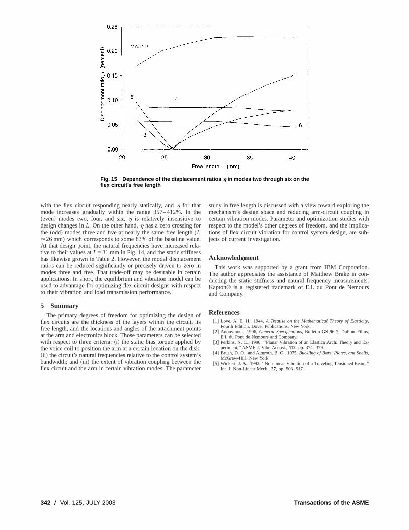
with the flex circuit responding nearly statically, andh for thatmode increases gradually within the range 357–412%. In the~even! modes two, four, and six,h is relatively insensitive todesign changes inL. On the other hand,h has a zero crossing forthe ~odd! modes three and five at nearly the same free length (L'26 mm) which corresponds to some 83% of the baseline value.At that design point, the natural frequencies have increased rela-tive to their values atL531 mm in Fig. 14, and the static stiffnesshas likewise grown in Table 2. However, the modal displacementratios can be reduced significantly or precisely driven to zero inmodes three and five. That trade-off may be desirable in certainapplications. In short, the equilibrium and vibration model can beused to advantage for optimizing flex circuit designs with respectto their vibration and load transmission performance.

5 SummaryThe primary degrees of freedom for optimizing the design of

flex circuits are the thickness of the layers within the circuit, itsfree length, and the locations and angles of the attachment pointsat the arm and electronics block. Those parameters can be selectedwith respect to three criteria:~i! the static bias torque applied bythe voice coil to position the arm at a certain location on the disk;~ii ! the circuit’s natural frequencies relative to the control system’sbandwidth; and~iii ! the extent of vibration coupling between theflex circuit and the arm in certain vibration modes. The parameter

study in free length is discussed with a view toward exploring themechanism’s design space and reducing arm-circuit coupling incertain vibration modes. Parameter and optimization studies withrespect to the model’s other degrees of freedom, and the implica-tions of flex circuit vibration for control system design, are sub-jects of current investigation.

AcknowledgmentThis work was supported by a grant from IBM Corporation.

The author appreciates the assistance of Matthew Brake in con-ducting the static stiffness and natural frequency measurements.Kapton® is a registered trademark of E.I. du Pont de Nemoursand Company.

References@1# Love, A. E. H., 1944,A Treatise on the Mathematical Theory of Elasticity,

Fourth Edition, Dover Publications, New York.@2# Anonymous, 1996,General Specifications, Bulletin GS-96-7, DuPont Films,

E.I. du Pont de Nemours and Company.@3# Perkins, N. C., 1990, ‘‘Planar Vibration of an Elastica Arch: Theory and Ex-

periment,’’ ASME J. Vibr. Acoust.,112, pp. 374–379.@4# Brush, D. O., and Almroth, B. O., 1975,Buckling of Bars, Plates, and Shells,

McGraw-Hill, New York.@5# Wickert, J. A., 1992, ‘‘Non-linear Vibration of a Traveling Tensioned Beam,’’

Int. J. Non-Linear Mech.,27, pp. 503–517.

Fig. 15 Dependence of the displacement ratios h in modes two through six on theflex circuit’s free length


M. SaigoResearch Manager,

Mechanical Engineering Laboratory,Agency of Industrial Science and Technology,

1-2 Namiki, Tsukuba, Ibaraki 305-8564, Japane-mail: [email protected]

K. TaniProfessor,

Gifu University,1-1 Yanagito, Gifu 501-1193, Japan


H. UsuiNippon Steel Corporation,

2-6-3 Otemati, Chiyodaku, Tokyo 100-8071,Japan


Vibration Control of a TravelingSuspended System Using WaveAbsorbing ControlThis paper describes vibration control of a suspended system using a wave absorbingmethod. Here, we treat a system that accepts a traveling command. This system is calleda traveling system. In the previous paper, we treated a system that performs only thevibration control, where the support of the suspended system moves only for vibrationcontrol and eventually settles at the original position. This system is called a nontravelingsystem. In a traveling system, the support moves both for traveling and for vibrationcontrol. We present a new control strategy for these two different aims by applying thevibration control method developed in the previous paper. A traveling multiple-pendulumsystem and a traveling wire-and-load system are treated. The wire-and-load system has asmall rigid pendulum between the support and the wire. The vibration control is per-formed by monitoring this small rigid pendulum. The wire-and-load system is extended toa model crane system that has a motor system to roll up and down the suspended masslike a real crane. The same program with different parameter values controls these threesystems. Both numerical simulation and experiment have been conducted, and the devel-oped control method has been shown to be quite effective.@DOI: 10.1115/1.1569515#

1 IntroductionRecently, traveling-wave control has been studied as an alter-

native to mode-based vibration control by several researchers.Wave control has several advantages over mode-based vibrationcontrol; it has no control and observation spillovers that may oc-cur in the vibration control when there are some imperfections insystem modeling or inaccuracy in sensor locations; it has a bettercontrol performance than vibration control at low frequencies; andit is basically a local control method to which we have paid atten-tion in our studies. The last feature means that we can suppress thevibration of a system using no more than the information aboutthe dynamic states of the element nearest the actuator. This isquite advantageous to the system whose parameters are change-able during control operations.

The studies of traveling-wave control include Vaughan@1#, VonFlotow @2,3#, Millar @4#, Mace @5#, Fujii @6#, Tanaka@7# and Ut-sumi @8#. These studies of traveling-wave control of elastic beamsor strings have used the theoretical solution expressed in the formof traveling wave and derived the nonreflecting condition ofwaves at the control point. On the other hand, O’Connor@9#treated a mass-and-spring system and presented a method of thewave-absorption in a discrete vibration system. In these studies,few attempts have been made to apply the wave control strategyto practical vibrating systems to show the above-mentioned ad-vantages of traveling-wave control.

In the previous paper@10#, we presented a new practical wavecontrol strategy that is easy to build in a control computer withon-line calculation of the imaginary wave-propagating system. Weapplied the presented method to the vibration suppression of amultiple-pendulum system and showed the effectiveness of themethod experimentally. There, vibration control by controlling thesupport movement was addressed and no support movement fortraveling toward a given target position was considered.

In the present paper, the wave control method presented in theprevious paper is expanded to consider the combination of travel-ing control and vibration control. In this case, the control systemhas to achieve a system displacement to a desired target position

while suppressing the vibration. Both a multiple-pendulum systemand a wire-and-load suspended system are treated. Furthermore,the method is applied to a model crane system and shown to beuseful for the vibration suppressing of a practical crane.

2 Equation of Motion

2.1 Multiple-Pendulum System. Figure 1 shows a travel-ing multiple rigid-pendulum system and a traveling wire-and-loadsystem. The equations of motion of a traveling multiple-pendulumsystem ofn degrees of freedom~DOF! are obtained using theLagrange’s equation of motion. The kinetic energyTk and thepotential energyUk of the k-th pendulum are expressed as

Tk5mkS y01 (j 5k11

n

l j u j D 2

/21I kuk2/21mkS y01 (

j 5k11

n

l j u j D ukhk

Uk52mkgH hk~12uk2/2!1 (

j 5k11

n

l j~12u j2/2!J

whereuk is the angle of thek-th pendulum numbered from thefree end and assumed to be so small that the terms having powershigher than second ofuk are negligible,hk is the distance betweenthe center of gravity of thek-th pendulum and the axis of thek-thconnecting pin,I k is the moment of inertia of thek-th pendulumabout the axis of thek-th connecting pin,mk is the mass ofk-thpendulum,l k is the distance between the axes of thekth and (k21)-th connecting pins, andy0 is the position of the support ofthe pendulum system. The LagrangianL5(k51

n (Tk2Uk) givesthe equations of motion ofk-th pendulum as

S I k1 l k2(

i 51

k21

mi D uk1 l k(j 51

k21 S l j(i 51

j 21

mi1hjmj D u j1S l k(i 51

k21

mi

1hkmkD (i 5k11

n

~ l i u i !1gS l k(i 51

k21

mi1hkmkD uk50 (1)

From the equations obtained by replacingk by k11 and byk21 in Eq. ~1!, as well as Eq.~1! itself, the following equation isobtained.

Contributed by the Technical Committee on Vibration and Sound for publicationin the JOURNAL OF VIBRATION AND ACOUSTICS. Manuscript received May 2000;Revised Jan. 2002. Associate Editor: R. L. Clark.


2$q1p11J1 /~r 1m1!%u11q2p1u21g~m11r 2m2!p1~2u11u2!

50

qk21pk21uk212@qkpk1$Jk1 l k~12r k21!mk21%pk21#uk

1qk11pkuk111gH S (j 51

k22

mj1r k21mk21D pk21uk21

2S (j 51

k21

mj1r kmkD ~pk1pk21!uk1S (j 51

k

mj

1r k11mk11D pkuk11J 50 ~kÞ1,n!

(2)

qn21pn21un212$Jn1 l n~12r n21!mn21%pn21un

1gpn21H S (j 51

n22

mj1r n21mn21D un212S (j 51

n21

mj

1r nmnD unJ 52 y0

r k5hk / l k , Jk5I k / l k , pk51/$~12r k!mk1r k11mk11%,

qk5Jk2hkmk

From the above equation, we see the term of the support move-ment appears explicitly only in the equation of the uppermostpendulum.

2.2 Wire-and-Load System. The wire-and-load systemshown in Fig. 1 has a small rigid pendulum between the supportand the wire, and there is a load at the bottom of the wire. Thewire length is fixed. Assuming the equation of the wire is ex-pressed by that of a dangling string and applying the finite differ-ence method to the equation of motion, we obtain a system ofequations similar to that of a multiple simple-pendulum system~see Appendix!. In the following numerical simulation, we willtreat the wire-and-load system as a non-homogenous multiple-pendulum system consisting of the uppermost rigid pendulum anda large-DOF series of simple pendulums, among them the lowesthaving a mass equal to that of the load.

3 Control StrategyThe concept of our vibration control is to connect the system

whose vibration should be suppressed to a virtually infinite systemthat can absorb vibration energy endlessly. In the previous paper,we have presented a control strategy in which the real pendulumsystem is suspended by the imaginary energy-absorbing multiple-pendulum system whose dynamics is simulated by on-line com-putation. Since we have to use a finite-DOF energy absorbingsystem in practice, we introduced initialization methods for theenergy absorbing system. At the time of initialization, the deflec-tions and velocities of all the imaginary pendulums other than thelowest are set to zero, and the deflection and velocity of the lowestare set to fit the present position and velocity of the support of thereal system.

In this paper, we treat vibration control of a suspended systemthat accepts a traveling command. The traveling command isgiven in term of the acceleration of the suspended systemyc as afunction of time. Two types of imaginary multiple-pendulum sys-tem are possible as shown in Fig. 2. One is the nontravelingimaginary system~NTIS, Fig. 2~a!! and the other the travelingimaginary system~TIS, Fig. 2~b!!. The NTIS does not accept thetraveling commandyc and thus its algorithm is the same as that ofthe vibration control of the non-traveling system treated in theprevious paper. The vibration control calculated using NTIS isadded with the traveling command to produce position control ofthe support of the real system. The influence of the traveling isactually regarded as a disturbance appearing on the uppermostpendulum of the real system. With TIS, on the other hand, thesupport of the imaginary system is moved according to the trav-eling commandyc and the movement is propagated through theimaginary system down to the real system. For both cases in Fig.2, the value ofx05(k51

n l kwk is the distance between the horizon-tal positions of the support and of the lowest end of the imaginarysystem. The initialization is performed based on this value.

Through numerical simulations we have found the control per-formance using NTIS is better than that using TIS. It is consideredthat the initialization using TIS brings about a larger initial deflec-tion and velocity to the lowest imaginary pendulum because theacceleration of the imaginary system due toyc produces a largervalue ofx0 . This causes the vibration energy flow back into thecontrolled real system. Therefore, we use NTIS in the followingwork.

Fig. 2 N-DOF imaginary system for traveling pendulum sys-tem „ y c : traveling command, x 0 : vibration control … „a… Non-traveling Imaginary System „NTIS…, „b… Traveling ImaginarySystem „TIS…

Fig. 1 Traveling multiple-pendulum system and wire-and-loadsystem


Three types of initializing timing are investigated for NTIS asshown in Fig. 3. The cases~a! and ~b! in Fig. 3 are the same asthose used in the previous paper, while~c! in Fig. 3 is a newmethod presented in this paper. In the case~a!, the PI method,initialization is made whenx050(5(k51

n l kwk), and in the case~b!, the VI method, initialization is made whenx050. In the case~c!, the VI’ method, initialization is made whenx050 as in thecase~b! but also has a position shift of the support of imaginarysystem. The vibration control performance in this case is betterthan in the cases~a! and ~b!, except that it may cause an error inthe final support position of the real system. It may be advanta-

geous first to move the system near the destination with less vi-bration and then to control the final position accurately. It is aneasy job for the control computer, given the present and targetpositions, to cancel the error of the final position.

When the real pendulum system is connected to the imaginarysystem, the acceleration of the lowest end of the imaginary systemis represented as

x05~ i 2/ l 2h!u1g~m01h/ l !u2g~11m01m!w

12h/ l 1m(3)

whereu is the angle of the uppermost rigid pendulum,w is theangle of the lowest imaginary system pendulum,m0 is the ratio ofthe mass of the total real system to that of the uppermost rigidpendulum,m is the ratio of the mass of an imaginary systempendulum to that of the uppermost rigid pendulum, andl, h andi 2

are the length, the distance between the supporting point and cen-ter of gravity, and the square of radius of gyration on the support-ing point, of the uppermost rigid pendulum, respectively. As statedfor the non-traveling case investigated in the previous paper,x0 isused here also as the control of the movement of the support ofthe real pendulum system for vibration suppression. A homog-enous multiple simple-pendulum system is used as the imaginarysystem in Eq.~3! for simplicity same as in the previous paper. Ameasured value ofu, the numerically approximated value ofu andthe computed value ofw from the imaginary system give thevibration controlx0 . Note that Eq.~3! includes no dimensionalparameters of the suspended pendulums except those of the up-permost one. So, it can give vibration control for the multiplerigid-pendulum system as well as for the wire-and-load systemwith an uppermost rigid pendulum. In other words, the controldoes not depend on the length of the wire.

The parameterm is introduced in Eq.~3! for the adjustment ofthe performance of the control system. For a large value ofm, thewave propagation in the imaginary system becomes slower andthe control gain for the vibration suppression smaller. A smallergain makes the control of the system more stable but less effec-tive. In the experiment, we obtained the practical values formconsidering the system stability and the limitations of the actualDC servo motor system. Thus, the wave propagating characteris-tics in the imaginary system and the control performance of thevibration suppression can be designed by changing the values ofm. The parameterk, the ratio of the length of the imaginary sys-tem pendulum to that of the uppermost rigid pendulum, can alsochange the wave propagating characteristics in the imaginary sys-tem.

4 Experiment

4.1 Experiments of the Multiple-Pendulum System andthe Wire-and-Load System

4.1.1 Experimental Apparatus.Figure 4 shows a schematicdiagram of the experimental apparatus. The uppermost pendulumis connected to and supported by the nut of the ball-screw. Theball-screw is driven by a 350W DC servomotor to generate thehorizontal movement of the support of pendulum. The DC servo-motor is a velocity feedback type with an integrated tacho-generator. A rotary encoder is attached to the uppermost pendu-lum.

The multiple-pendulum system is made of three same-size alu-minum plates connected serially by pins allowing free rotation.The width and thickness of each plate are 40 mm and 10 mm,respectively. The distance between the center axes of the connect-ing pins of each plate is 300 mm. The adjacent plates can be fixedrigidly with braces to form a pendulum system having less thanthree degrees of freedom.

The wire-and-load system is made up of a rigid pendulum, awire and a load. The length, width and thickness of the rigid

Fig. 3 Three types of initializing method for NTIS. „a… PImethod: initialization when x 0Ä0, „b… VI method: initializationwhen x 0Ä0, „c… VI’ method: initialization when x 0Ä0 with sup-port shift


pendulum are 60 mm, 40 mm and 15 mm, respectively. The di-ameter of the wire is 1 mm. The length of the wire and the weightof the load can be changed.

The computation of the control is conducted by a DSP~TMS320C30! for the rigid-pendulum system and a personal com-puter with 200 MHz CPU for the wire-and-load system. The sam-pling period of A/D conversion is 0.1 ms for the rigid-pendulumsystem and 2 ms for the wire-and-load system. A 10-DOF systemof simple pendulums has been used as the imaginary system.

4.1.2 Experimental Results.The following system move-ment pattern is used as the traveling command in the experiments;the accelerationyc is 4.26 m/s2 for the time period between 0 sand 0.0352 s and20.01883 m/s2 between 0.0352 s and 8 s. Usingthis acceleration pattern the pendulum system should travel thedistance of 0.60 m in 8 seconds.

„a… The case of the multiple-pendulum systemFigures 5 show the effects of the different initializing methods,

the PI and VI’ methods, for the 3-DOF traveling rigid-pendulumsystem withm53. In these figures, the curve rising to the right-hand side is the position of the support and the vibration wave-form is the angle of the uppermost pendulum. From these figures,we can confirm that our method is effective for a traveling pen-dulum system as well as for a nontraveling system. Figures 6show the control performance of the PI method and the VI’method on the 1-DOF pendulum system~three pendulums areconnected rigidly!. Both initializing methods have excellent vibra-tion suppressing effects. Similarly, the control performance on thenon-homogeneous 2-DOF pendulum system~the lowest and themiddle pendulums are connected rigidly! is well confirmed~fig-ures are not shown!. The control program for the 2-DOF system isthe same as that for the 3-DOF system, for the uppermost pendu-lum and the total mass of the system are the same.„b… The case of the wire-and-load systemFigures 7 show the effects of the different initializing methods,

the PI and VI’ methods, for the traveling wire-and-load systemwith the wire lengthl 50.5 m, the load weightw512.3 N andm53. In these figures, the curve rising to the right-hand side is theposition of the support and the vibration waveform is the angle ofthe uppermost pendulum. From these figures we can see that theVI’ method has quite an excellent damping performance~Fig.7~c!!. The PI method is accurate in positioning the pendulum sys-tem at the traveling destination, but the vibration control perfor-mance is not so good. The performance of the VI method is not sogood~figure is not shown!. The vibration waveform shown in Fig.7~c! resembles well that of the 1-DOF rigid pendulum shown inFig. 6~b!. This means the dynamic characteristics of the experi-mental wire-and-load system is similar to that of the 1-DOF rigid-

pendulum system and the vibration of the wire is practically neg-ligible. Figures 8 show the effect of the wire lengthl and the loadweight w on the control performance of the VI’ method whenm51. We can see the control performance is independent of thechange of the wire length and the load weight. Besides, the con-trol performances in Fig. 8 form51 are better than that in Fig.7~c! for m53, which confirms that the quick wave propagation inthe imaginary system brings about a better performance in vibra-tion suppression while the system is stable.

Fig. 4 Experimental apparatus „wire-and-load system …

Fig. 5 Experimental results of 3 DOF rigid-pendulum system„mÄ3, kÄ1…. „a… No control, „b… Control with PI method, „c… Con-trol with VI’ method

Fig. 6 Experimental results of 1 DOF rigid-pendulum system„mÄ1, kÄ1…. „a… Control with PI method, „b… Control with VI’method


Figures 9 show the results of the operation in which final posi-tioning accuracy is concerned when the VI’ method is used forvibration control. As stated earlier, this method can produce apositioning error, and some measures should be taken when accu-rate positioning at the target is needed. Figure 9~a! is an overruncase where the vibration control is switched to the VI method andthe traveling command is suppressed the instant the supportreaches the exact target position. Figure 9~b! is a case where thepositioning correction to the exact target position is carried outusing the VI method after the traveling command is over. Either

process can position the support accurately at the target positionwith small vibration. Figure 10 shows a non-traveling case wherea combination of initializing methods is used for a large initialamplitude. This process combines the PI method that absorbsquickly large amplitudes with the VI method that absorbs quicklysmall amplitudes. The PI method was used between 0 s and 6 sand the VI method was used afterwards. This, combinations ofdifferent initialization methods can be used effectively to adapt tovarious situations.

In order to understand the characteristics of the initializingmethods obtained in the experiments, several numerical simula-tions have been conducted. Figures 11 show the simulation resultsfor the wire-and-load system corresponding to Fig. 7~b! and~c!. Inthe simulation, dry friction is assumed at each connecting pin ofthe pendulum to represent the wire. The ratio of the mass of thewire to that of the uppermost pendulum is assumed to be 0.0001.Small wire vibrations occur at the starting period in the simulationresults, which are not observed in the experiments. In Fig. 11 weshow the waveform of the swing angle of the load in stead of thatof the uppermost pendulum because the latter is affected by thesmall wire vibration. There is little difference between the resultsin Fig. 11 and Fig. 7. From these figures, we can confirm that theexperiments have been performed successfully and that the angleof the uppermost rigid pendulum is virtually equal to the swingangle of the load.

As is easily understood, the vibration of the load would propa-gate up to the uppermost rigid pendulum. So, our wave-absorbingsystem, which attends the uppermost rigid pendulum, is eventu-ally effective in suppressing the vibration of the load.

Fig. 7 Experimental results of wire-and-load system „ lÄ0.5 m, wÄ12.3 N, mÄ3, kÄ10…. „a… No control, „b… Control withPI method, „c… Control with VI’ method

Fig. 8 Experimental results of wire-and-load system for differ-ent wire length and load weight with VI’ method „mÄ1,kÄ10…. „a…lÄ0.3 m, wÄ12.3 N „b… lÄ0.9 m, wÄ31.9 N

Fig. 9 Experimental results of wire-and-load system for finalpositioning „ lÄ0.3 m, wÄ12.3 N, mÄ10, kÄ10…. „a… Interruptionof traveling command „overrun case …, „b… Position correctionafter traveling command

Fig. 10 Experimental result of nontraveling wire-and-load sys-tem for large amplitude with PI and VI methods „ lÄ0.3 m, wÄ12.3 N, mÄ10, kÄ10….


The VI’ method shows best vibration suppression among thethree initializing methods. The PI and VI methods have inferiorvibration control performances, especially for a small value ofm.Therefore, it is suitable to use a relatively large value ofmdepressing the vibration control performance for the PI or VImethods.

4.2 Experiment of a Model Crane

4.2.1 Experimental Apparatus.Figure 12 shows the experi-mental model of a crane, which has a load suspended by a wireand a pulley. One end of the wire is fixed to the motor shaft forwinding and the other end is fixed to a small rigid pendulum thatis attached to the nut of the ball-screw with free rotation. Thedistance between the axis of the rigid pendulum and the wirereturn on the returning pulley is equal to the diameter of the pul-ley. Then, the angle of the rigid pendulum is practically equal tothe swing angle of the load independent of its height when thesmall vibrations of the wire can be ignored. This means the sta-

tionary direction of the pendulum is always vertical and the vibra-tion suppression strategy for the wire-and-load system is applieddirectly by monitoring one half of the load suspension system.Our experiment has shown that it is possible to neglect the smallwire vibration in the wire-and-load system as well as in mostpractical crane systems. The velocity pattern used of winding-upand rewinding-down is 0.1 m/s and20.1 m/s, respectively. Theload moves between the vertical positions of 0.9 m and 0.3 mduring the time period between 0 s and 6 s.

4.2.1 Experimental Results.Figures 13 show the experimen-tal results for the case of winding up the load;~a! in Fig. 13 is thecase where no vibration control is used,~b! is the case with wavecontrol in the PI method, and~c! is the case with wave control inthe VI’ method. Figures 14 show the cases of rewinding down theload with controls similar to those in Fig. 13. The system move-ment pattern is the same as in the case for the wire-and-loadsystem. In Fig. 13 we can see the amplitude of the vibration inwinding-up without control becomes larger as the wire length be-comes shorter, due to the instability in winding-up of a suspendedload. The contrast in these figures demonstrates the effectivenessof the stabilization using the wave-absorbing control. In addition,the wave control method presented has shown an excellent controlperformance regardless of the wire length. Figures 13~b! and14~b! with the PI method for a large value ofm show relativelygood results in the final state of the load, that is, accurate finalposition and small vibration. Thus, we can use the PI method toposition the system accurately at the target position if its vibrationsuppression performance is acceptable. Even if the VI’ method is

Fig. 11 Numerical results of wire-and-load system „ lÄ0.5 m,wÄ12.3 N, mÄ3, kÄ10…. „a… Control with PI method, „b… Controlwith VI’ method

Fig. 12 Model crane system

Fig. 13 Experimental results of crane system for raising load„total weight Ä17.6N…. „a… No control, „b… Control with PI method„mÄ10, kÄ10…, „c… Control with VI’ method „mÄ1, kÄ10…


used, the final position errors are not very significant. Figures 13and 14 have shown our wave absorbing method is useful for theactual crane system.

5 Concluding RemarksIn this paper we propose a wave control method using a non-

traveling imaginary multiple-pendulum system applied to vibra-tion control of the traveling suspended system. We have shownthat the method presented, using little information about the sus-pended system states, is quite effective for a traveling suspendedsystem whose dynamics are changeable during operation. The ini-tializing methods with and without shifting the support of theimaginary system have their respective merits for the application.The former realizes accurate final positioning while the latter re-alizes excellent vibration suppression. Combination of methodscan produce excellent overall performances. This control methodcan readily be applied to real crane systems that have a movingpulley and parallel wiring.

Nomenclature

g 5 Gravitational acceleration(*˙ ), (*¨ ) 5 first and second order differentiation with respect

to timei 2 5 square of radius of gyration on the supporting

point of the uppermost rigid penduluml 5 length of the uppermost rigid pendulumh 5 distance between the supporting point and the

center of gravity of the uppermost rigid pendulumm0 5 ratio of the mass of the total real system to that of

the uppermost rigid pendulum

m 5 ratio of the mass of an imaginary system pendu-lum to that of the uppermost rigid pendulum

k 5 ratio of the length of an imaginary system pendu-lum to that of the uppermost rigid pendulum

u 5 angle of the uppermost rigid pendulumw 5 angle of the lowest imaginary system pendulum

uk 5 angle of thek-th rigid pendulum numbered fromthe free end

hk 5 distance between the center of gravity ofk-thrigid pendulum and the axis ofk-th connectingpin

I k 5 moment of inertia ofk-th rigid pendulum aboutthe axis ofk-th connecting pin

mk 5 mass ofk-th rigid penduluml k 5 distance between the axes of thek-th and

(k21)-th connecting pins of the rigid pendulumwk 5 angle of thek-th imaginary system pendulum

numbered from the lowest endx0 5 (k51

n l kwk ~n: degrees of freedom of imaginarysystem!

y0 5 horizontal displacement of the support~imaginaryor real!

yc 5 traveling commandh 5 deflection of the wire

h i 5 deflection of thei-th finite element of the wirez 5 coordinates of the wire measured from the lower

~free! end

AppendixWe assume the equation of motion of the wire is expressed by

that of a dangling string. By balancing the horizontal componentof forces on an infinitely small elementz;(z1dz), the followingequation is obtained as

S M

r1zD ]2h

]z21

]h

]z2

1

g

]2h

]t250 (A1)

whereh is the lateral deflection of wire,z is the coordinate mea-sured from the lowest end,r is the mass of string per unit lengthandM is the mass of load.

Appling the finite difference method to the above equation us-ing the following approximations,

]2h

]z25

h i 1122h i1h i 21

Dz2,

]h

]z5

h i2h i 21

Dz, z5 iDz

we obtain

M

rDz~h i 2122h i1h i 11!1~ i 21!h i 212~2i 21!h i1 ih i 11

5Dz

gh i (A2)

where h i is the lateral deflection ofi-th mesh point numberedfrom the lowest end of the wire andDz is the finite differencemesh.

From Eq.~A2! and the equation obtained by replacingi by i11 in Eq. ~A2!, we obtain the following equation of motion bysubstitutingu i5(h i2h i 11)/Dz,

Dz

gu i5

M

rDz~u i 1122u i1u i 21!1~ i 21!u i22iu i1~ i 11!u i 11

(A3)

The above equation is the same as the equation of motion of amultiple simple-pendulum system obtained from Eq.~2! if weregardDz as the length of the simple pendulum andM as theadditional mass to the lowest pendulum. This means that we cansimulate the dynamics of wire in the form of a system of simplependulums of lengthDz.

Fig. 14 Experimental results of crane system for lowering load„total weight Ä17.6 N…. „a… No control, „b… Control with PI method„mÄ10, kÄ10…, „c… Control with VI’ method „mÄ1, kÄ10…


The influence of a wire on the total dynamics of the pendulumsystem is quite small as can be seen in the experimental results.The exact dynamical formulation for a wire is not so important inour study~M is much greater thanrDz). So, we will not try todevelop a more accurate mathematical model of the wire in thispaper.

References@1# Vaughan, D. R., 1968, ‘‘Application of Distributed Parameter Concepts to

Dynamic Analysis and Control of Bending Vibrations,’’ ASME J. Basic Eng.,90, pp. 157–166.

@2# Von Flotow, A. H., 1986, ‘‘Traveling Wave Control for Large Spacecraft Struc-tures,’’ AIAA J., 9, pp. 462–468.

@3# Von Flotow, A. H., 1986, ‘‘Disturbance Propagation in Structural Networks,’’J. Sound Vib.,106, pp. 433–450.

@4# Miller, D. W., and von Flotow, A. H., 1989, ‘‘A Travelling Wave Approach toPower Flow in Structural Networks,’’ J. Sound Vib.,128, pp. 145–162.

@5# Mace, B. R., 1984, ‘‘Wave Reflection and Transmission in Beams,’’ J. SoundVib., 97, pp. 237–246.

@6# Fujii, H., and Ohtsuka, T., 1992, ‘‘Experiment of a Noncollocated Controllerfor Wave Cancellation,’’ AIAA J.,15~3!, pp. 93–97.

@7# Tanaka, N., and Kikushima, Y., 1992, ‘‘Active Wave Control of a FlexibleBeam,’’ JSME Int. J., Ser. III,35~1!, pp. 236–244.

@8# Utsumi, M., 1999, ‘‘Analytical Implementation of Wave-Absorbing Controlfor Flexible Beams Using Synchronization Condition,’’ASME J. Vibr. Acoust.,121, pp. 468–475.

@9# O’Connor, W., and Lang, D., 1998, ‘‘Position Control of Flexible Robot ArmsUsing Mechanical Waves,’’ ASME J. Dyn. Syst., Meas., Control,120, pp.334–339.

@10# Saigo, M., Tanaka, N., and Tani, K., 1998, ‘‘An Approach to Vibration Controlof Multiple-Pendulum System by Wave Absorption,’’ ASME J. Vibr. Acoust.,121, pp. 524–533.


J. R. BanerjeeProfessor of Structural Dynamics,

School of Engineeringand Mathematical Sciences,

City University, Northampton Square, LondonEC1V OHB


Dynamic Stiffness Formulationand Its Application for aCombined Beam and a TwoDegree-of-Freedom SystemThis paper is concerned with the dynamic stiffness formulation and its application for aBernoulli-Euler beam carrying a two degree-of-freedom spring-mass system. The effect ofa two degree-of-freedom system kinematically connected to the beam is represented ex-actly by replacing it with equivalent stiffness coefficients, which are added to the appro-priate stiffness coefficients of the bare beam. Numerical examples whose results are ob-tained by applying the Wittrick-Williams algorithm to the total dynamic stiffness matrixare given and compared with published results. Applications of the theory include the freevibration analysis of frameworks carrying two degree-of-freedom spring-masssystems.@DOI: 10.1115/1.1569943#

1 IntroductionThere are many important engineering structures that can be

modelled as beams carrying one, two or multi degree-of-freedomspring-mass systems. Examples of such practical applications in-clude components of buildings and machine tools, vehicle suspen-sions, rotating machinery, accessories of machine structures androbotics amongst others. Because of these wide-ranging applica-tions the vibration behavior of beams carrying discrete structuralelements such as a one, two or multi degree-of-freedom spring-mass systems has received considerable attention for many years.The research has developed from the simpler problem of the freevibration analysis of beams with lumped masses@1–9# or springsupports@10–16# to that of beams carrying elastically mountedmasses@17–25# or a one or two degree of freedom spring-masssystems@26–31#. ~For further reading on combined dynamicalsystems in general, Refs.@32#, @33# are recommended.! All theseinvestigations have shown that the natural frequencies and modeshapes of a beam carrying spring-mass systems may deviate con-siderably from those of the beam alone.

The main drawback of the existing solution procedures for suchproblems is that by and large they concentrate solely on uniformand unidirectional beams, and cannot be generally applied toframeworks. This paper presents an entirely different approachbased on the dynamic stiffness method which is free from suchlimitations and yields exact results, some of which can be directlycompared to the solution of the complete governing differentialequations. It does not seem to be widely recognized that the dy-namic stiffness method allows an assembly technique~similar tothat used in finite element methods! that enables exact free vibra-tion analysis of either a single structural element or a combinationof structural elements with different orientations. Furthermore, incontrast to finite element methods, the results using the dynamicstiffness method are not only exact, but also independent of thenumber of elements used in the analysis and thus offers muchbetter computational efficiency.

The free vibration analysis of simple beams or frameworks hasbeen solved using the dynamic stiffness method without difficulty@34,35#, because the dynamic stiffness properties of a beam@36#and the solution technique known as Wittrick-Williams algorithm@37# are both well established. The method also allows a concen-

trated or lumped mass/inertia, or a spring, to be added at a node orjoint of a structure@38#, without compromising the accuracy, andhence retaining the exactness of results. However, a difficultyarises when the beam is attached to a discrete structural elementsuch as a two degree-of-freedom system because the member dy-namic stiffness matrix, the basic building block in the method ofsuch a combined system, is not currently available. This paperdevelops the dynamic stiffness matrix of a Bernoulli-Euler beamto which has been attached a two degree-of-freedom spring-masssystem, which is free to translate and rotate. The resulting eigen-values of the combined system, which yield the natural frequen-cies of the combined structure, are determined using the Wittrick-Williams algorithm@37#. In order to illustrate the method severalcases have been evaluated and some representative results havebeen compared with published ones. This paper is thought to bethe first in which the dynamic stiffness matrix of a combination ofcontinuous and discrete structural elements has been developed.Although the simple case of the Bernoulli-Euler beam has beenconsidered here as the parent structural member for illustrativepurposes, the procedure is completely general and can easily beextended to Timoshenko beams with or without an axial load@39–42# carrying a two degree-of-freedom spring-mass system.

2 Theory

2.1 Dynamic Stiffness Formulation for a Bernoulli-EulerBeam. The dynamic stiffness matrix of a Bernoulli-Euler beamhas been available in the literature@34,36# for many years. Ban-erjee@43# has given a general formulation that leads to the devel-opment of the dynamic stiffness matrix of a structural element.For a Bernoulli-Euler beam the procedure is simple and is de-scribed as follows.~Readers who are not familiar with the subjectare referred to the Appendix, which gives details of the dynamicstiffness development.! In both axial and transverse motion thegoverning partial differential equations in free vibration are de-rived, and the corresponding total differential equations for har-monic motion established. These are then integrated in terms oftwo arbitrary constants for axial motion, and in terms of four morefor the flexural motion. The associated end loads are then obtainedin terms of the arbitrary constants, so that for the longitudinalmotion, the axial force at each end, as well as the axial displace-ments are both expressible in terms of the two arbitrary constants.Eliminating the two constants then gives the relationship betweenthe two end forces and two end displacements. This embodies the

Contributed by the Technical Committee on Vibration and Sound for publicationin the JOURNAL OF VIBRATION AND ACOUSTICS. Manuscript received May 2002;Revised Dec. 2002. Associate Editor: B. Yang.


~frequency dependent! dynamic stiffness matrix for axial motionrelating the amplitudes of forces and displacements at the ends ofthe freely vibrating Bernoulli-Euler beam.

In a similar way, the shear force and bending moment at eachend of the beam, together with the bending displacement and ro-tation at each end, are expressible in terms of four constants ofintegration when dealing with the free vibration in flexural mo-tion. On eliminating these constants, a relationship between thefour end loads and the four kinematic conditions at the ends, isestablished. The resulting 434 matrix linking the two is the fre-quency dependent dynamic stiffness matrix in flexural motion.

The axial and flexural dynamic stiffness properties can now becompounded into a 636 dynamic stiffness matrix of theBernoulli-Euler beam, relating the amplitudes of the forces to thecorresponding amplitudes of the displacements at the ends of thevibrating beam~see Fig. 1!. In the usual notation when the beamparametersEA, EI, m and L represent the extensional rigidity,bending rigidity, mass per unit length and length of the beamrespectively, the dynamic stiffness matrix takes the followingform ~see Appendix for details!

F Fx1

Fy1

M1

Fx2

Fy2

M2

G53a1 0 0 a2 0 0

0 d1 d2 0 d4 d5

0 d2 d3 0 2d5 d6

a2 0 0 a1 0 0

0 d4 2d5 0 d1 2d2

0 d5 d6 0 2d2 d3

4 FU1

V1

u1

U2

V2

u2

G (1)

or

F5Kd (2)

whereF andd are respectively the force and displacement vectorsandK is the frequency dependent dynamic stiffness matrix whoseelementsk( i , j ) ( i 51,2 . . . 6; j 51,2, . . . 6). aregiven bya1 , a2andd12d6 .

In Eq. ~1!, Fx1 , Fy1 , M1 andU1 , V1 andu1 are the amplitudesof the forces and displacements at end 1 andFx2 , Fy2 , M2 andU2 , V2 andu2 are the corresponding amplitudes of the forces anddisplacements at end 2, respectively~see Fig. 1!. The elements ofthe dynamic stiffness matrixa1 , a2 and d12d6 are as follows~see Appendix for details!.

a15EA

Lm cotm, a252

EA

Lm cos ecm (3)

with

m5Amv2L2

EA(4)

and

d15W3l3~SlChl1ClShl!/D, d25W2l2SlShl /D,

d35W1l~SlChl2ClShl!/D(5)

d452W3l3~Sl1Shl!/D, d55W2l2~Chl2Cl!/D,

d65W1l~Shl2Sl!/D

with

W15EI

L, W25

EI

L2, W35

EI

L3(6)

l5A4 mv2L4

EI(7)

Cl5cosl, Sl5sinl, Chl5coshl, Shl5sinhl (8)

and

D512ClChl (9)

2.2 Dynamic Stiffness Formulation for a Two Degree-of-Freedom Spring-Mass System Attached to a Beam.Figure 2shows a rigid massM having a mass moment of inertiaI a aboutits centroidal axis and mounted at the ends~nodes! of a Bernoulli-Euler beam by means of two linearly elastic springs of springconstantKS1 andKS2 , respectively. The distances of the center ofgravity ~g! of the mass from the location of the springs areD1 andD2 respectively, as shown.

The governing differential equations of motion for the twodegree-of-freedom spring mass system shown in Fig. 2, undergo-ing free vibration in translation and rotation, are

M]2vM

]t22 f k12 f k250 (10)

I a

]2aM

]t21 f k1D12 f k2D250 (11)

where vM and aM are the transverse displacement and angularrotation of the rigid mass,t is time, andf k1 and f k2 are the inter-active spring forces between the spring-mass system and the beamat the two connecting points at nodes 1 and 2 respectively~seeFig. 2!. These forces are given by

f k15KS1~v12vM1D1aM ! (12)

f k25KS2~v22vM2D2aM ! (13)

wherev1 andv2 are the transverse bending displacements of thebeam at nodes 1 and 2 respectively.

If harmonic oscillation with circular~or angular! frequencyv isassumed, then

vM~x,t !5VMeivt, aM~x,t !5AMeivt,

Fig. 1 Amplitudes of displacements and forces at the ends ofa Bernoulli-Euler Beam in free vibration

Fig. 2 A two degree-of-freedom system kinematically con-nected to a beam element


v1~x,t !5V1eivt, v2~x,t !5V2eivt (14)

and

f k1~x,t !5Fk1eivt, f k2~x,t !5Fk2eivt (15)

whereVM , AM , V1 , V2 , Fk1 andFk2 are the amplitudes of freevibration.

Substituting Eqs.~14! and ~15! into Eqs.~10!–~13! gives

~2Mv21KS11KS2!VM1~KS2D22KS1D1!AM

2KS1V12KS2V250 (16)

~2KS1D11KS2D2!VM1$2I av21~KS1D121KS2D2

2!%AM

1KS1D1V12KS2D2V250 (17)

Equations~16! and ~17! are solved forVM andAM to give

VM5@KS1$KS2D2~D11D2!2I av2%V1

1KS2$KS1D1~D11D2!2I av2%V2#/Z (18)

AM5@KS1$D1Mv22KS2~D11D2!%V1

1KS2$KS1~D11D2!2D2Mv2%V2#/Z (19)

where

Z5MI av42v2$KS1~ I a1D12M !1KS2~ I a1D2

2M !%

1KS1KS2~D11D2!2 (20)

From Eqs.~12! and~13! the spring force amplitudes are given by

Fk15KS1~V12VM1D1AM ! (21)

Fk25KS2~V22VM2D2AM ! (22)

With the expressions forVM andAM given by Eqs.~18! and~19!,Eqs.~21! and~22! can now be written in terms ofV1 andV2 only,in the form

FFk1

Fk2G5Fe1 e2

e2 e3G FV1

V2G (23)

where, after some reduction,e1 , e2 ande3 are given by

e15KS1v2$MI av22KS2~ I a1D22M !%/Z (24)

e25KS1KS2v2~ I a2D1D2M !/Z (25)

e35KS2v2$MI av22KS1~ I a1D12M !%/Z (26)

Equation~23! provides the required dynamic stiffness matrix ofthe two degree-of-freedom system~see Fig. 2! wheree1 , e2 ande3 are the equivalent stiffnesses linking forces which will be trans-mitted to the beam at nodes 1 and 2 to the associated displace-mentsV1 and V2 . The stiffnesses account for the attached twodegree-of-freedom system properly, and no approximation is in-volved in their derivation.

The above analysis enables a two degree-of-freedom springmass system to be represented exactly by essentially a pair ofsprings, loading the beam at nodes 1 and 2 with stiffnesses vary-ing dynamically according to Eq.~23!.

2.3 Dynamic Stiffness Matrix of the Combined Bernoulli-Euler Beam and the Two Degree-of-Freedom Spring-MassSystem. The dynamic stiffness matrix of the combinedBernoulli-Euler beam and the two degree-of-freedom system cannow be obtained by incorporating the dynamic stiffness force-displacement relationship of the two degree-of-freedom system ofEq. ~23! into the dynamic stiffness force-displacement relation-ship of the Bernoulli-Euler beam given by Eq.~1!. This is realizedby adding respectively,e1 to k(2,2) term,e2 to k(2,5) term,e2 tok(5,2) term ande3 to k(5,5) term of the stiffness matrixK of Eqs.~1!–~2!. Thus the modified force displacement relationship of thecombined dynamical system can be written as

F Fx1

Fy11Fk1

M1

Fx2

Fy21Fk2

M2

G53a1 0 0 a2 0 0

0 d11e1 d2 0 d41e2 d5

0 d2 d3 0 2d5 d6

a2 0 0 a1 0 0

0 d41e2 2d5 0 d11e3 2d2

0 d5 d6 0 2d2 d3

43F U1

V1

u1

U2

V2

u1

G (27)

or

F5Kd (28)

whereK , F, andd are the modified dynamic stiffness matrix, andforce and displacement vectors respectively.

3 Application of the Dynamic Stiffness MatrixThe dynamic stiffness matrix of Eqs.~27!–~28! can now be

used to compute the natural frequencies and mode shapes of eithera single beam with various end conditions or an assembly ofbeams, for example a plane or space frame, carrying one or moretwo degree-of-freedom spring-mass systems. When several ele-ments are to be used the overall dynamic stiffness matrix of thecomplete structure must be assembled. The associated natural fre-quencies and mode shapes are then extracted using the Wittrick-Williams algorithm, see Refs.@37# and @34,35#. The algorithmguarantees that no natural frequency and its associated mode aremissed. This is, of course, not possible in the conventional finiteelement method. Interested readers will fill the procedure detailedin Refs. @34,35,37#. Note that the algorithm requires informationabout the clamped-clamped natural frequencies of all elements@34,35,37# within the structure to provide exact results. For thepresent problem the determination of the clamped-clamped natu-ral frequencies of the structural element shown in Fig. 2 willinvolve the calculation of natural frequencies of the Bernoulli-Euler beam as well as those of the two degree-of-freedom systemwhen both ends~nodes 1 and 2! are built-in. The frequency equa-tion for a Bernoulli-Euler beam with clamped-clamped end con-ditions can be derived using standard procedure@44# whereas forthe two degree-of-freedom system connected to the Bernoulli-Euler beam shown in Fig. 2, the corresponding clamped-clampednatural frequencies can be obtained by substitutingZ50 of Eq.~20!. In order to ensure that no natural frequencies of the structureare missed the actual requirement for applying the Wittrick-Williams algorithm @37# is to identify how many such clamped-clamped natural frequencies exist below an arbitrarily chosen trialfrequency rather than calculating them precisely@34,35,43#.

4 Numerical Results and DiscussionTo illustrate the above theory two examples are given. The first

is taken from Ref.@28# in which a beam clamped at both endscarries a two degree-of-freedom spring-mass system as shown inFig. 3. The data used in the analysis are as follows:

EA53.031010 N, EI56.253108 Nm2,

m51179 kg/m, L151.4 m, L251.2 m,

L351.4 m, M5200 kg, I a570.833 kgm2,

D15D250.6 m and KS15KS251010 N/m

The first three natural frequencies of the beam in flexural vibrationare shown in Table 1 together with those reported in Ref.@28# and


also with those obtained with the two degree-of-freedom spring-mass system missing. Except for the second natural frequency theresults agreed completely with those of Ref.@28# in which aLaplace transformation technique with respect to the spatial vari-able is used, and is expected to give exact results. The author wasunable to pin-point the exact reason for the small discrepancy~less than 0.04%! in the second natural frequency, but this may beattributed to the accuracy used in the input data of Ref.@28#. InRef. @28# the built-in end conditions were simulated by using verylarge linear and rotational springs~of the order of 1020) and arethought unlikely to alter the results. The mode shapes correspond-ing to these first three natural frequencies are shown in Fig. 4,which agree very well with the ones illustrated in Fig. 3 of Ref.@28#.

Although the present theory is capable of determining the natu-ral frequencies in axial vibration, these were suppressed by disal-lowing the axial deformation of the beam, so that the results aredirectly comparable with those of Ref.@28#. The axial naturalfrequencies are uncoupled from the bending ones and they are notof interest as they will remain unaffected by the presence of thetwo degree-of-freedom spring-mass system.~If the spring connec-tions are oblique or the two degree-of-freedom system is con-nected to a framework a coupling would occur in which case theaxial motion of the beam would have to be included in the analy-sis.! The results of Table 1 show that the presence of the twodegree-of-freedom spring-mass system has changed the first threenatural frequencies by 3.43%, 3.97% and 0.05%, respectively. Ofcourse, any change in the natural frequencies will be dependent onthe parameters of the two degree-of-freedom spring-mass systemand its location on the beam.

The next set of results for this example was obtained to dem-onstrate the effect of the spring constantsKS1 ~or KS2) on thefundamental natural frequency of the beam.~Note thatKS1 andKS2 are equal for the present problem.! Figure 5 shows the varia-tion of the fundamental natural frequency (v1) of the beamagainst the variation of the spring constantKS1 ~or KS2). Forsmaller values of stiffness coefficients the fundamental naturalfrequency increases with the increase in spring constant, but be-yond a large stiffness constant it approaches a steady~constant!value and remains virtually unaltered. This is to be expected andis in accord with an earlier investigation@28#. Other parameters

Fig. 3 A clamped-clamped beam carrying a two degree-of-freedom spring-mass system

Fig. 4 The first three natural frequencies and mode shapes ofthe clamped-clamped beam carrying a two degree-of-freedomshown in Fig. 3

Fig. 5 The effect of spring stiffness on the fundamental natu-ral frequency of the clamped-clamped beam carrying a twodegree-of-freedom shown in Fig. 3

Table 1 Natural frequencies of a combined beam and a twodegree-of-freedom system

Frequency Number

Natural frequencies~rad/s!

Combined beam and two DOF system

Beam alonePresent theory Ref.@28#

1 983.19 983 1018.12 2695.1 2694 2806.43 5499.0 5499 5501.8


such as the lengths of the beam segments (L1 , L2 andL3) and/orthe mass and mass moment of inertia~M and I a) of the twodegree-of-freedom system, see Fig. 3, can also be varied and theirsubsequent effects on the natural frequencies can be studied. Adetailed investigation of this type is beyond the scope of thispaper because it will no-doubt take it further than it is intended.However, it should be stressed that the proposed method enables aparametric study to be made to position appropriately the naturalfrequencies within or without a certain band. This may sometimesbe necessary to avoid resonance, for example in the mounting of amachine.

The second illustrative example is a plane frame consisting ofbeam members as shown in Fig. 6. One of the structural memberscarries a two degree-of-freedom spring-mass system as shown.The natural frequencies of the frame without the two degree-of-freedom spring-mass system have been obtained by Howson andWilliams using a published computer program@34# based on thedynamic stiffness matrix method. However, when the two degree-of-freedom spring-mass system is included the problem becomesvery different and cannot generally be solved using earlier ap-proaches. The application of the present theory is particularly use-ful for solving such problems. As in Ref.@34# it is assumed thateach member~beam! of the frame shown in Fig. 6 has the sameproperties which are as follows:

EA58.03108 N, EI54.03106 Nm2 and m530 kg/m

The length of each member of the frame can be deduced from thegeometry shown. The parameters of the two degree-of-freedomsystem connected to one of the members in the frame as shown inFig. 6 are

M51500 kg, I a575 kgm2, KS15108 N/m,

KS251.253108 N/m, D15D251.5 m.

The nodes of the frame are numbered as shown. Following theusual procedure generally used in the finite element method, thedynamic stiffness matrix of the complete frame is assembled fromthe dynamic stiffness matrices of all the individual elements in theframe. Of course, for the element connecting the nodes 2 and 4,the dynamic stiffness theory developed in this paper is used. Thefirst three natural frequencies of the frame including and exclud-ing the two degree-of-freedom system were obtained using theWittrick-Williams algorithm and are shown in Table 2 togetherwith the percentage difference between the two sets of results.~The published program of Howson and Williams@34# gives thesame natural frequencies as the present theory when the two

degree-of-freedom system is ignored.! The results shown in Table2 indicate that the natural frequencies vary significantly as a resultof the attached two degree-of-freedom system.

5 ConclusionsA dynamic stiffness matrix for a combined beam and a two

degree-of-freedom spring-mass system is developed starting fromthe classical differential equation theory of its free natural vibra-tion. By applying the Wittrick-Williams algorithm the resultingdynamic stiffness matrix is used to determine the free vibrationcharacteristics of a beam and a plane frame which are kinemati-cally connected to a two degree-of-freedom spring-mass system.The results for the beam carrying a two degree-of-freedom spring-mass system agreed with published results. The theory allows anynumber of two degree-of-freedom spring-mass systems to beadded to a structure consisting of beams. This useful extension ofthe dynamic stiffness method to combined system to cover frame-works is the context in which the theory is expected to be mostadvantageous, particularly in the avoidance or attenuation of un-welcome vibration. The method used is exact and can be appliedto validate finite element or other approximate methods.

Appendix

Derivation of the Dynamic Stiffness Matrix of a Bernoulli-Euler Beam. The axial and bending deformations for aBernoulli-Euler beam are uncoupled. Therefore, the derivation ofthe dynamic stiffness matrix for each of these two cases can becarried out separately, and later can be combined together.

Axial Stiffnesses. A uniform Bernoulli-Euler beam of lengthLis shown in Fig. 7 in a rectangular right handed Cartesian co-ordinate system with the X-axis coinciding with the axis of thebeam. The governing differential equation of motion of the beamin free axial~or longitudinal! vibration is given by@36,44#

EA]2u

]x22m

]2u

]t250 (A1)

whereEA andm are the axial~or extensional! rigidity and massper unit length of the beam respectively, andu(x,t) is the axialdisplacement of the cross-section at a distancex, andt is time.

Fig. 6 A plane frame carrying a two degree-of-freedom springmass system

Fig. 7 Coordinate system and notation for a Bernoulli-Eulerbeam

Table 2 Natural frequencies of a plane frame carrying a twodegree-of-freedom system

FrequencyNumber

Natural frequency~rad/s!

%difference

Frame withtwo DOF system

Frame withouttwo DOF system

1 176.62 224.76 21.42 229.40 245.70 6.633 246.09 267.38 7.96


Assuming harmonic oscillation with angular~or circular! fre-quencyv so that

u~x,t !5u~j,t !5U~j!eivt (A2)

where U(j) is the amplitude of axial vibration andj5x/L.Substituting Eq.~A2! into Eq. ~A1! gives

d2U

dj21m2U50 (A3)

where

m5Amv2L2

EA(A4)

The solution of the differential Eq.~A3! is given by

U~j!5C1 cosmj1C2 sinmj (A5)

whereC1 andC2 are constants.The expression for axial forceF(x) in the positive direction of

X ~see Fig. 7! can be expressed with the help of Eq.~A5! as

F~x!5F~j!52EAdU

dx52

EA

L

dU

dj

5EA

Lm~C1 sinmj2C2 cosmj! (A6)

Now referring to Fig. 8~a!, the boundary~or end! conditions fordisplacements and forces can be applied as follows.

At x50 ~ i.e. j50!, U5U1 and F5Fx1 (A7)

At x5L ~ i.e. j51!, U5U2 and F52Fx2 (A8)

Substituting Eqs.~A7! and ~A8! into Eqs.~A5! and ~A6!, the fol-lowing matrix relationships can be obtained

FU1

U2G5F 1 0

cosm sinmG FC1

C2G (A9)

and

FF1

F2G5 EA

LmF 0 21

2sinm cosmG FC1

C2G (A10)

The constantsC1 andC2 can now be eliminated from Eqs.~A9!and~A10! to give the dynamic stiffness formulation of the axiallyvibrating beam relating amplitudes of the forces and displace-ments at its ends as follows

FFx1

Fx2G5Fa1 a2

a2 a1G FU1

U2G (A11)

where the frequency dependent elements of the 232 dynamicstiffness matrix are given by

a15EA

Lm cotm, a252

EA

Lm cos ecm (A12)

Bending Stiffnesses.The governing differential equation ofmotion of the Bernoulli-Euler beam shown in Fig. 7 in bending~or flexural! natural vibration is given by@36,44#

EI]4v

]x41m

]2v

]t250 (A13)

whereEI andm are the bending~or flexural! rigidity and mass perunit length of the beam respectively, andv(x,t) is the bending~orflexural! displacement of the cross-section at a distancex and t istime.

Assuming harmonic oscillation with angular~or circular! fre-quencyv so that

v~j,t !5V~j!eivt (A14)

whereV(j) is the amplitude of bending~or flexural! vibration andj5x/L. Substituting Eq.~A14! into Eq. ~A13! gives

d4V

dj42l4V50 (A15)

where

l5A4 mv2L4

EI(A16)

The solution of the differential Eq.~A15! is given by@36,44#

V~j!5C3 coslj1C4 sinlj1C5 coshlj1C6 sinhlj(A17)

whereC3–C6 are constants.The expressions for rotation~u!, bending moment~M! and

shear force~S! consistent with the positive direction of the co-ordinate system at the left hand end of the beam can be written as

u~x!5u~j!51

L

dV

dj5

l

L~2C3 sinlj1C4 coslj1C5 sinhlj

1C6 coshlj! (A18)

M ~x!5M ~j!52EI

L2

d2V

dj25

EI

L2l2~C3 coslj1C4 sinlj

2C5 coshlj2C6 sinhlj!

(A19)

S~x!5S~j!5EI

L3

d3V

dj35

EI

L3l3~C3 sinlj2C4 coslj

1C5 sinhlj1C6 coshlj! (A20)

Now referring to Fig. 8~b!, the boundary~or end! conditions forthe displacements and forces can be applied as follows

At x50 ~ i.e. j50!, V5V1 , u5u1 , S5Fy1

and M5M1 (A21)

At x5L~ i.e. j51!, V5V2 , u5u2 , S52Fy2

Fig. 8 End conditions for a Bernoulli-Euler beam in free vibra-tion


and M52M2 (A22)

Substituting Eqs.~A21! and~A22! into Eqs.~A17!–~A20!, the fol-lowing two matrix equations can be obtained for displacementsand forces, respectively, in terms of the constantsC3–C6 .

F V1

u1

V2

u2

G5F 1 0 1 0

0 l/L 0 l/L

Cl Sl Chl Shl

2lSl /L lCl /L lShl /L lChl /L

GF C3

C4

C5

C6

G(A23)

and

F Fy1

M1

Fy2

M2

G5F 0 2W3l3 0 W3l3

W2l2 0 2W2l2 0

2W3l3Sl W3l3Cl 2W3l3Shl 2W3l3Chl

2W2l2Cl 2W2l2Sl W2l2Chl W2l2Shl

G3F C3

C4

C5

C6

G (A24)

where

Cl5cosl, Sl5sinl, Chl5coshl, Shl5sinhl,

W15EI

L, W25

EI

L2, W35

EI

L3(A25)

The constantsC3–C6 can now be eliminated to give the 434dynamic stiffness matrix of the Bernoulli-Euler beam in flexuralvibration as follows

F Fy1

M1

Fy2

M2

G5F d1 d2 d4 d5

d2 d3 2d5 d6

d4 2d5 d1 2d2

d5 d6 2d2 d3

GF V1

u1

V2

u2

G (A26)

where

d15W3l3~SlChl1ClShl!/D, d25W2l2SlShl /D,

d35W1l~SlChl2ClShl!/D (A27)

d452W3l3~Sl1Shl!/D, d55W2l2~Chl2Cl!/D,

d65W1l~Shl2Sl!/D (A28)

with

D512ClChl (A29)

Combination of Axial and Bending Stiffnesses.A simple su-perposition is now possible to put the axial and bending dynamicstiffnesses together in order to express the force-displacement re-lationship of the Bernoulli-Euler beam. Superposing Figs. 8~a!and 8~b!, see Fig. 1, and using Eqs.~A11! and~A26!, one obtainsthe dynamic stiffness relationship of a Bernoulli-Euler beam infree vibration, as follows

F Fx1

Fy1

M1

Fx2

Fy2

M2

G53a1 0 0 a2 0 0

0 d1 d2 0 d4 d5

0 d2 d3 0 2d5 d6

a2 0 0 a1 0 0

0 d4 2d5 0 d1 2d2

0 d5 d6 0 2d2 d3

4 FU1

V1

u1

U2

V2

u2

G(A30)

or

F5Kd (A31)

whereF andd are respectively the force and displacement vectorsandK is the frequency dependent 636 dynamic stiffness matrixwhose elementsk( i , j ) ( i 51,2 . . . 6; j 51,2, . . . 6) aregiven bya1 , a2 andd12d6 defined in Eqs.~A12!, ~A27! and ~A28!. Notethat K is symmetric as expected.

References@1# Chen, Y., 1963, ‘‘On the Vibration of Beams or Rods Carrying a Concentrated

Mass,’’ ASME J. Appl. Mech.,30, pp. 310–311.@2# Pan, H. H., 1965, ‘‘Transverse Vibration of an Euler Beam Carrying a System

of Heavy Bodies,’’ ASME J. Appl. Mech.,32, pp. 434–437.@3# Laura, P. A. A., Pombo, J. L., and Susemihl, E. A., 1974, ‘‘A Note on the

Vibration of a Clamped-Free Beam with a Mass at the Free End,’’ J. SoundVib., 37, pp. 161–168.

@4# Parnell, L. A., and Cobble, M. H., 1976, ‘‘Lateral Displacements of a VibratingCantilever Beam with a Concentrated Mass,’’ J. Sound Vib.,44, pp. 499–511.

@5# Gurgoze, M., 1984, ‘‘A Note on the Vibrations of Restrained Beams and Rodswith Point Masses,’’ J. Sound Vib.,96, pp. 461–468.

@6# Burch, J. C., and Mitchell, T. P., 1987, ‘‘Vibration of a Mass-Loaded Clamped-Free Timoshenko beam,’’ J. Sound Vib.,114, pp. 341–345.

@7# Laura, P. A. A., Filipich, C. P., and Cortinez, V. H., 1987, ‘‘Vibrations ofBeams and Plates Carrying Concentrated Masses,’’ J. Sound Vib.,117, pp.459–465.

@8# Wu, J. S., and Lin, T. L., 1990, ‘‘Free Vibration Analysis of a Uniform Can-tilever Beam with Point Masses by an Analytical-and-Numerical-CombinedMethod,’’ J. Sound Vib.,136, pp. 201–213.

@9# Abramovich, H., and Hamburger, O., 1991, ‘‘Vibration of a Cantilever Ti-moshenko Beam with a Tip Mass,’’ J. Sound Vib.,148, pp. 162–170.

@10# Massalas, C., and Soldatos, K., 1978, ‘‘Free Vibration of a Beam Subjected toElastic Constraints,’’ J. Sound Vib.,57, pp. 607–608.

@11# Davies, H. G., and Rogers, R. J., 1979, ‘‘The Vibration of Structures Elasti-cally Constrained at Discrete Points,’’ J. Sound Vib.,63, pp. 437–447.

@12# Lau, J. H., 1981, ‘‘Fundamental Frequency of a Constrained Beam,’’ J. SoundVib., 78, pp. 154–157.

@13# Verniere, P., Ficcadenti, G., and Laura, P. A. A., 1984, ‘‘Dynamic Analysis ofa Beam with an Intermediate Elastic Support,’’ J. Sound Vib.,96, pp. 381–389.

@14# Lau, J. H., 1984, ‘‘Vibration Frequencies and Mode Shapes for a ConstrainedCantilever,’’ ASME J. Appl. Mech.,51, pp. 182–187.

@15# Maurizi, M. J., and Bambill de Rossit, D. V., 1987, ‘‘Free Vibration of aClamped-Clamped Beam with an Intermediate Elastic Support,’’ J. Sound Vib.,119, pp. 173–176.

@16# Rao, C. K., 1989, ‘‘Frequency Analysis of Clamped-Clamped Uniform Beamswith Intermediate Elastic Support,’’ J. Sound Vib.,133, pp. 502–509.

@17# Jacquot, R. G., and Gibson, J. D., 1972, ‘‘The Effects of Discrete Masses andElastic Supports on Continuous Beam Natural Frequencies,’’ J. Sound Vib.,23,pp. 237–244.

@18# Laura, P. A. A., Maurizi, M. J., and Pombo, J. L., 1975, ‘‘A Note on theDynamic Analysis of an Elastically Restrained-Free Beam with a Mass at theFree End,’’ J. Sound Vib.,41, pp. 397–405.

@19# Laura, P. A. A., Susemihl, E. A., Pombo, J. L., Luisoni, L. E., and Gelos, R.,1977, ‘‘On the Dynamic Behavior of Structural Elements Carrying ElasticallyMounted, Concentrated Masses,’’ Appl. Acoust.,10, pp. 121–145.

@20# Bapat, C. N., and Bapat, C., 1987, ‘‘Natural Frequencies of a Beam withNonclassical Boundary Conditions and Concentrated Masses,’’ J. Sound Vib.,112, pp. 177–182.

@21# Ercoli, L., and Laura, P. A. A., 1987, ‘‘Analytical and Experimental Investiga-tion on Continuous Beams Carrying Elastically Mounted Masses,’’ J. SoundVib., 114, pp. 519–533.

@22# Larrondo, H., Avalos, D., and Laura, P. A. A., 1992, ‘‘Natural Frequencies of aBernoulli Beam Carrying an Elastically Mounted Concentrated Mass,’’ OceanEng.,19, pp. 461–468.

@23# Abramovich, H., and Hamburger, O., 1992, ‘‘Vibration of a Cantilever Ti-moshenko Beam with Translational and Rotational Springs and with TipMass,’’ J. Sound Vib.,154, pp. 67–80.

@24# Rossi, R. E., Laura, P. A. A., Avalos, D. R., and Larrondo, H. O., 1993, ‘‘FreeVibrations of Timoshenko Beams Carrying Elastically Mounted, ConcentratedMasses,’’ J. Sound Vib.,165, pp. 209–223.

@25# Gurgoze, M., 1996, ‘‘On the Eigenfrequencies of a Cantilever Beam withAttached Tip Mass and a Spring-Mass System,’’ J. Sound Vib.,190, pp. 149–162.

@26# Jen, M. U., and Magrab, E. B., 1993, ‘‘Natural Frequencies and Mode Shapesof Beams Carrying a Two-Degree-of-Freedom Spring-Mass System,’’ ASMEJ. Vibr. Acoust.,115, pp. 202–209.

@27# Wu, J. S., and Huang, C. G., 1995, ‘‘Free and Forced Vibrations of a Timosh-enko Beam with any Number of Translational and Rotational Springs andLumped Masses,’’ Int. J. Commun. Num. Meth. Eng.,11, pp. 743–756.

@28# Chang, T. P., and Chang, C. Y., 1998, ‘‘Vibration Analysis of Beams with aTwo Degree-of-Freedom Spring-Mass System,’’ Int. J. Solids Struct.,35, pp.383–401.

@29# Wu, J. S., and Chou, H. M., 1998, ‘‘Free Vibration Analysis of a CantileverBeam Carrying any Number of Elastically Mounted Pointed Masses with the


Analytical-and-Numerical-Combined Method,’’ J. Sound Vib.,213, pp. 317–332.

@30# Wu, J. S., and Chou, H. M., 1999, ‘‘A New Approach for Determining theNatural Frequencies and Mode Shapes of a Uniform Beam Carrying any Num-ber of Sprung Masses,’’ J. Sound Vib.,220, pp. 451–468.

@31# Wu, J. J., and Whittaker, A. R., 1999, ‘‘The Natural Frequencies and ModeShapes of a Uniform Beam with Multiple Two-DOF Spring-Mass Systems,’’ J.Sound Vib.,227, pp. 361–381.

@32# Dowell, E. H., 1979, ‘‘On Some General Properties of Combined DynamicalSystems,’’ ASME J. Appl. Mech.,46, pp. 206–209.

@33# Nicholson, J. W., and Bergman, L. A., 1986, ‘‘Free Vibration of CombinedDynamical Systems,’’ J. Eng. Mech.,112, pp. 1–13.

@34# Howson, W. P., and Williams, F. W., 1977, ‘‘Compact Computation of NaturalFrequencies and Buckling Loads for Plane Frames,’’ Int. J. Numer. MethodsEng.,11, pp. 1067–1081.

@35# Howson, W. P., Banerjee, J. R., and Williams, F. W., 1983, ‘‘Concise Equationsand Program for Exact Eigensolutions of Plane Frames including MemberShear,’’ Adv. Eng. Software,5, pp. 137–141.

@36# Kolousek, V., 1973,Dynamics in Engineering Structures, Butterworths, Lon-don.

@37# Wittrick, W. H., and Williams, F. W., 1971, ‘‘A General Algorithm for Com-puting Natural Frequencies of Elastic Structures,’’ Q. J. Mech. Appl. Math.,24,pp. 263–284.

@38# Anderson, M. S., Williams, F. W., Banerjee, J. R., Durling, B. J., Herstrom, C.L., Kennedy D., and Warnaar, D. B., 1986, ‘‘User Manual BUNVIS-RG: AnExact Buckling and Vibration Program for Lattice Structures, with RepetitiveGeometry and Substructuring option,’’ NASA Tech. Memo. 87669.

@39# Cheng, F. Y., 1970, ‘‘Vibration of Timoshenko Beams and Frameworks,’’ J.Struct. Div. ASCE,96, pp. 551–571.

@40# Wang, T. M., and Kinsman, T. A., 1971, ‘‘Vibration of Frame Structures Ac-cording to the Timoshenko Theory,’’ J. Sound Vib.,14, pp. 215–227.

@41# Howson, W. P., and Williams, F. W., 1973, ‘‘Natural Frequencies of Frameswith Axially Loaded Timoshenko Members,’’ J. Sound Vib.,26, pp. 503–515.

@42# Cheng, F. Y., and Tseng, W. H., 1973, ‘‘Dynamic Stiffness Matrix of Timosh-enko Beam Columns,’’ J. Struct. Div. ASCE,99, 527–549.

@43# Banerjee, J. R., 1996, ‘‘Dynamic Stiffness Formulation for Structural Ele-ments: A General Approach,’’ Comput. Struct.,63, pp. 101–103.

@44# Clough, R. W., and Penzien, J., 1975,Dynamics of Structures, McGraw-Hill,Singapore.


Paolo GallinaAssociate Professor,

Department of Energetics,University of Trieste,

Via A. Valerio 10-34127 Trieste, Italye-mail: [email protected]

Effect of Damping on AsymmetricSystemsThis paper addresses the phenomenon of the destabilizing effect of slight damping onasymmetric linear systems. Previous works had showed that the destabilizing effect, re-garded for a long time as a ‘‘paradox,’’ depends upon the ratio of the damping coeffi-cients. This work extends those results to n-dof systems. In fact, conditions for a generalasymmetric n-dof slightly damped system to be stable are obtained. Also, a useful suffi-cient condition is carried out. This practical design tool gives optimum damping ratiosand takes into consideration the parameter uncertainties as well. The solution is based onthe eigenvalue sensitivity analysis. Moreover, a formal physical explanation of the desta-bilizing effect of damping is given. Eventually, the theory is validated by means of asimple example.@DOI: 10.1115/1.1569945#

1 IntroductionThe dynamic behavior of a general linear discrete undamped

system can be described by a vector differential equation of theform

Mx ~ t !1Kx ~ t !50 (1)

whereM andK are the mass and stiffness matrices respectively.If mass and stiffness matrices are symmetric positive definite,

the system is stable in the BIBO sense, where the acronym BIBOstands for ‘‘bounded input bounded output.’’ In most cases, thedamping matrix is neglected as far as stability analysis is con-cerned. In fact, the structural damping of the real system wouldhave the effect of moving the eigenvalues of the undamped sys-tem toward the negative complex plane.

If the mass and/or the stiffness matrices are asymmetric, theundamped system can be either stable or unstable. This type ofdynamic systems can be found in aeronautics, active control oflarge structures, vehicle dynamics and milling machining@1,2#. Inthese circumstances, neglecting the damping matrix is no longerpossible.

Because of the asymmetry of the matrices, a destabilizing effectdue to the damping matrix could arise. This atypical phenomenon,regarded for a long time as a ‘‘paradox’’@3# has been physicallyexplained by Semler et al.@4#. Using a 2 d.o.f. example, Semlershowed that damping introduces two effects: it dissipates energyand it modifies the modes of vibration. The latter could cause thework done by the external forces to increase. If the work done bythe external forces becomes greater than the energy dissipated bydamping, the system will be unstable.

Bolotin @5# showed how the destabilizing effect of slight damp-ing is related to the ratio of the damping coefficients. This resultwas carried out for a 2 d.o.f. asymmetric system. Studying a lin-earized double pendulum with a follower force, Herrmann et al.@6,7# achieved similar results. Using an approximated method,Nemat-Nasser@8#, showed the destabilizing effect of damping ona cantilevered continuous pipe conveying fluid. The approach headopted can be extended to 3 d.o.f systems. Unfortunately, allthose works focus on particular examples with few degrees offreedom. This paper extends the theory to a generaln-dof asym-metric linear slightly damped system. If the undamped system isstable, all the eigenvalues are located on the imaginary axis. Theintroduction of slight damping modifies the location of the eigen-values of the system on the complex plane. By means of an ei-genvalue sensitivity analysis@9#, one can foresee which direction

the eigenvalues will move. We proved that destabilizing effect dueto slight damping occurs when a system of homogeneous linearinequalities is not satisfied. This general condition is an extensionof the results obtained by Bolotin@5#, Herrmann et al.@6#

The paper is divided into three parts: in the first one a detailedanalysis of slight damping effects on a generaln-dof stable un-damped system is carried out. A stability condition is obtained.Moreover, using the cone algorithm@10#, a simplified sufficientcondition for the slight damped system to be stable is obtained.This result is of practical interest because it gives the optimumdamping ratios for the system to be stable. Damping coefficientuncertainties are taken into account as well.

In the second part, a physical explanation of the destabilizingeffect of damping is given for a generaln-dof system, which ex-tends the result obtained by Semler@4# Eventually, the proposedmethod is explained and validated by means of a simple example.

2 Theory

2.1 Sensitivity Eigenvalue Analysis. Consider the system

Mx ~ t !1Cx~ t !1Kx ~ t !50 (2)

whereM andK are realn3n asymmetric matrices. The dampingmatrix C can be decomposed into a product of a matrixU and ascalarc, namelyC5cU, wherec5iCi and U5C/iCi. C is as-sumed symmetric andU inherits this symmetry.

Note that the system~2! can be always arranged so that thedamping matrix is symmetric. In fact, ifC was not symmetric, itis always possible to decompose the damping matrix using thesingular value decomposition method, namelyC5SCV, whereSandV are square matrices andC is a symmetric matrix. Therefore,the system~2! can be written in the formM x(t)1Cx(t)1Kx(t)50 whereM5S21MV 21, K5S21KV 21 andC is symmetric.

By means of the decompositioncU, one can calculate the ei-genvalues of the system as a function ofc. If c50, Eq. ~2! rep-resents the equation of the undamped system. Asc increases, thedamping matrix will affect the dynamic behavior of the system. Inthis way one can study the effect of a slight damping by introduc-ing a smallc. Since$U% i j 5$C% i j /c, each component ofU repre-sents adamping ratio. Note that, for definition, all the dampingratios are constant. For the sake of clarity, we will callU dampingratio matrix andc damping.

In the following, we answer this simple but fundamental ques-tion: If the undamped system is stable, will the introduction of thedamping destabilize the system? In order to answer the question,one can find where the eigenvectors move on the complex planeasc changes.

Contributed by the Technical Committee on Vibration and Sound for publicationin the JOURNAL OF VIBRATION AND ACOUSTICS. Manuscript received Sept. 2001;Revised Jan. 2003. Associate Editor: J. Cusumano.


The right eigenvalue problem associated with Eq.~2! can berepresented by

~Ml i21Cl i1K !ui50 (3)

wherel i , ui are respectively theith eigenvalue and theith righteigenvector of the system. In the same way, the left eigenvectorproblem is given by the equation

viT~Ml i

21Cl i1K !50 (4)

wherevi is the ith left eigenvector of the system.Differentiating Eq.~3! with respect to the dampingc, one ob-

tains

S 2Ml i

dl i

dc1Ul i1C

dl i

dc Dui1~Ml i21Cl i1K !

dui

dc50 (5)

Premultiplying by the left eigenvalueviT , it yields

viTS 2Ml i

dl i

dc1Ul i1C

dl i

dc Dui1viT~Ml i

21Cl i1K !dui

dc

5viTS 2Ml i

dl i

dc1Ul i1C

dl i

dc Dui50 (6)

Therefore the derivative of theith eigenvalue calculated forc50 is

dl i

dc52

viT~Ul i !ui

viT~2Ml i1C!ui

Uc50

52vi

TUui

2viTMu i

(7)

Eq. ~7! is a simple tool for foreseeing the effect of damping. Infact, if Re(dli /dc).0, a smallc will move theith eigenvaluel i ofthe undamped system (l i belongs to the complex axis since theundamped system is supposed to be stable in a BIBO sense! to-ward the right complex plane, causing the system to become un-stable. Conversely, if

Re~dl i /dc!,0, (8)

a smallc will move the ith eigenvalue toward left, causing thesystem to remain stable. Therefore, for smallc, the damping ratiomatrix will have a ‘‘stabilizing effect’’ only if Re(dli /dc),0 ;i51, . . . ,n. Note that the eigenvectors of an undamped system arealways real. Therefore, for this reason and for Eq.~7!

ReS dl i

dc D5dl i

dc(9)

We now apply the condition~8! to the following simple example.Consider the systemMx1cUx1Kx50, with the matrix

M5F3 2

1 3G K5F5 1.5

4 10G U5F2 0

0 1G (10)

The Undamped system (c50) is stable in the sense of BIBOstable. Its eigenvalues arel151.4684i , l2521.4684i , l351.7074i , l3521.7074i . The right and left eigenvectors of theundamped system are

u15F20.73270.3825 G , u25F20.7327

0.3825 G , u35F 0.652620.5645G ,

u45F 0.652620.5645G

(11)

v15F20.646620.5148G , v25F20.6466

20.5148G , v35F20.240020.8289G ,

v45F20.240020.8289G

Therefore

dl1

dc5

dl2

dc52

v1TUu1

2v1TMu1

520.5263

dl3

dc5

dl4

dc52

v3TUu3

2v3TMu3

520.1162 (12)

In conclusion, for a small value ofc, the stable undamped systemwill remain stable

2.2 An Alternative Simpler Way to Express Stability Con-ditions. Instead of Eq.~7!, by expanding matrixU, we can ob-tain a simplified formulation. For the sake of clarity, we introduceFig. 1, where part of a discrete mass-spring-damped system isrepresented. In this way one can visualize the physical meaning ofthe elements of the matrixU. In other words, Fig. 1 shows thedamping coefficients one can introduce in the mechanical system.The forces that cause the stiffness matrix and/or the mass matrixto be asymmetric are not depicted in figure.

We can now study the structure of the damping ratio matrixUand give its physical interpretation. This provides the designerwith an important tool to select the best combination of dampingelements. Basically, one has two different ways to introduce adamping element on a mechanical system:

• a damping element can be connected between one mass/inertia and the frame;

• a damping element can be connected between two masses/inertias.

The former is represented in the figure by a physical dampingelement attached between the massml and the frame. Its numeri-cal damping value iscj l l . We call damping element coefficientthe adimensional coefficientj l l .

In this case, ifcj l l was the only damping element on the me-chanical system, the matrixU would be

U5Ul l 5H $Ul l %o,p50 ;o,pÞ l

$Ul l %o,p5j l l o5p5 l5F 0 ¯ ¯ 0

] � ]

j l l

] � ]

0 ¯ ¯ 0

G(13)

where the notation$ %o,p indicates the element of the matrix onthe oth row andpth column.

Since the system hasn degrees of freedom, it is possible toconnect up ton damping elements between each mass/inertia andthe frame.

If cj ls was the only damping elements introduced between themassml and the massms the matrixU would be

Fig. 1 Mechanical example of a n d.o.f. system. Nonconserva-tive forces that cause the mass matrix and Õor the damping ma-trix to be asymmetric are not depicted in figure. A dampingelement can be inserted between two masses and Õor betweenone mass and the frame.


U5Uls5H $Uls%o,p50 ;oÞ l ,oÞs,pÞ l ,pÞs$Uls% l ,l5$Uls%s,s5j ls

$Uls% l ,s5$Uls%s,l52j ls

5F 0 ¯ ¯ 0

] j ls 0 2j ls ]

0

] 2j ls 0 j ls ]

0 ¯ ¯ 0

G (14)

In a n d.of. system, the number of possible damping elementsattached between one mass and another one is (n(n21))/2.Therefore the sum of the number of the possible damping ele-ments attached to the frame plus the number of the possible damp-ing elements attached between two masses isn1(n(n21))/25(n(n11))/2. In many cases, the number of damping elementsin a real mechanical system is less than (n(n11))/2.

Using a compact notation and considering all the damping ele-ment coefficients at the same time, one can compose the dampingratio matrix

U5(r 51

n

Urr 1 (r ,t51r .t

n

Urt5 (r ,t51r>t

n

Urt (15)

Multiplying by the ith right eigenvalue and premultiplying by theith left eigenvalue, it yields

viTUui5(

r 51

n

viTUrr ui1 (

r ,t51r .t

n

viTUrtui

5(r 51

n

$vi% r$ui% rj rr 1 (r ,t51r .t

n

~$vi% r$ui% r2$vi% r$ui% t

2$vi% t$ui% r1$vi% t$ui% t!j rt (16)

where the symbol$ % r means therth component of a vector. It isclear from the Eq.~16! that vi

TUui is a linear combination of thedamping element coefficientsj r ,r ,j r ,t (r ,t51, . . . ,n,r .t).Therefore, one can write

viTUui5ai

Tj (17)

where

ai5F $vi%1$ui%1

]

$vi%n$ui%n

$vi%1$ui%22$vi%1$ui%22$vi%2$ui%11$vi%2$ui%2

]

$vi%n21$ui%n2$vi%n21$ui%n2$vi%n$ui%n211$vi%n$ui%n

Gand the vectorjPRr (r 5((n(n11))/2)) gathers the damping co-efficients

jT5@j11,j22, . . . ,jnn ,j12,j13, . . . j1n ,j23, . . . ,j~n21!n#(18)

By replacing Eq.~17! into ~7!, one obtains the derivative of theitheigenvalue as a function of the damping element coefficient vector

dl i

dc52

aiTj

2viTMu i

(19)

Therefore

dl i

dc,0⇔sign~vi

TMu i !aiTj.0 (20)

In order the derivatives of the eigenvalues to be negative, thefollowing system of linear inequalities has to be satisfied

Aj.0 (21)

whereA¹Rn3r is

A5F sign~v1TMu1!a1

T

]

sign~vnTMun!an

TG (22)

In conclusion, instead of Eq.~8!, the stability condition is nowreplaced by the system of inequalities~21!. They present the ad-vantage that damping element coefficients appear explicitly.Therefore damping elements can be easily chosen in order main-tain the system stable.

Example:Considering again the numerical example~10!, wherej1152,

j2251, one obtains

A5F 0.4737 20.1969

0.4737 20.1969

20.1566 0.4679

20.1566 0.4679

Gand Eq.~20! becomes

A$j11 j22%T5$0.7505 0.7505 0.1547 0.1547%T.0 (23)

Eq. ~23!, according to Eq.~12! confirms again that the slightlydamped system is stable

2.3 A Simpler Sufficient Condition for Stability „SolutionCone…. Although condition~21! is useful to directly foresee thestabilizing or destabilizing effect of the damping element coeffi-cients, it is not of practical use for the mechanical designer.

The main reason is that system~21! has an infinite number ofsolutions. A method to choose the ‘‘best solution’’ of~21! amongthe possible alternatives is desirable.

We now introduce the notationai5sign(viTMu i)ai . From a

geometrical point of view, all the infinite solutions of~21! can beobtained in the following way. Each vectorai can be thought of asthe normal vector to an homogeneous hyperplane inRr . The hy-perplane bounds the halfplaneSi5$juai

Tj.0,j¹Rr%. The inter-section of ther halfplanes generates the solution setS of system~21! S5ù i 51

r Si . It is well known that the solution region is aconvex polyhedral cone inRr @11#. Introducing the definition ofsolution coneone can find a subset of solutions of system~21!.

A hypercone@10# with axis w andangleu in Rr is defined as

C~w,u!5$ju^w,j&,u,jPRr% (24)

where^w,j&5arccos~w"j/~iwiiji!! is the angle betweenw andj.A solution coneis a hypercone enclosed by the solution setS. Onecan find thelargest solution coneenclosed by the solution set. Theset of all the angles of the cones enclosed byS is

Dsc5$uuC~w,u!PS,wPRr ,uPR% (25)

Therefore, the angle of the largest solution cone isusc5max$Dsc% and its axis is

wsc5$wuC~w,usc!PS,wPRr% (26)

The largest solution cone can be found using thecone algorithmproposed by Wan@10#. A modified version of thecone algorithmis proposed in appendix. Since the largest solution cone is thelargest cone included inS, it gives a set of solutions of system~21!. Of course, it does not represent all the possible solutions; itdefines a subset of the solutions of the system of inequalities. Inspite of that, one can note that, while system~21! is made up ofrinequalities, the largest solution cone is defined by means of onlyone inequality:


arccosS wscT

iwsci•

j

iji D ,usc⇔wsc

T

iwsci• j.cos~usc! (27)

where j5j/iji. Moreover, only two parameters are necessary toexpress the condition:wsc , usc . Equation~27! is a powerful andsimple tool for designing the damping matrix. The damping ma-trix will stabilize the undamped system~under the hypothesis ofslight damping! if Eq. ~27! is satisfied. If one could choose thedamping element coefficients, the best solution would be

jopt5wsc

iwsci(28)

In fact, whenj5 jopt the value of the scalar productwscT /iwsci

• j51 of Eq. ~27! is maximum.Not only can the designer choose the best solution, but he also

can analyze the robustness of the solution.In a practical scenario model errors occur. Therefore, the real

value ofj defers from the theoretical optimum solutionjopt . Onecan take into account the uncertainties in the model by means ofthe relationship

j5 jopt6D j (29)

By replacing Eq.~29! into Eq. ~27!, we can express the stabilitycondition as a function of the uncertainty vectorDj

i joptT D ji,12cos~usc! (30)

Using Eq.~30!, given the optimum choice for the damping coef-ficients, one can analyze the effect of the uncertainties as far asrobustness of the system is concerned. In other words, as long asuncertainties satisfy Eq.~30!, the damped system is stable.

Resuming the example~10!, suppose now that the dampingelement coefficientsj11, j22 have to be set by the designer. Theoptimum solution provided by the cone algorithm is

[email protected] 0.6875#T, usc524.3° (31)

and the damping element uncertainties have to satisfy Eq.~30!

0.7262Dj1110.6875Dj22,0.0886 (32)

3 A General Physical Explanation of the DestabilizingEffect of Damping

In this section we explain in a elegant way the destabilizingeffect of damping from a physical point of view. We show thatthere exist modes of vibration that extract energy from the reser-voir of the system. In order to be excited these modes need anenergy sink where the system dissipates part of the energy bymeans of damping. We will prove that, when the slightly dampedsystem is unstable, the energy acquired by these modes is greaterthan the dissipated energy.

The mass and stiffness matrices of system~2! can be alwaysdecomposed in symmetric positive definite matrices and non sym-metric matrices, namelyM5M s1DM andK5K s1DK . There-fore the system~2! can be rewritten in the form

M sx~ t !1cUx~ t !1K sx~ t !52~DMx ~ t !1DKx ~ t !! (33)

SinceM s andK s are positive definite, system~33! can be thoughtof as a conservative system subjected the external forces2(DMx (t)1DKx (t)).

Given the ith eigenvalue and right eigenvector of the systeml i , ui , one mode of vibration of the system is given by

x51

2~uie

l i t1uiel i t! (34)

whereui , li are the complex conjugated ofui , l i5s i1 iv i . Togain a better understanding of the energy exchanges, consideronly the imaginary part of the eigenvalue in order to neglect theexponential term of the mode of vibration. In this way we con-

sider only the steady periodic part of the solution. In the followingwe calculate the energy the system exchanges during each cycle.

x>1

2~uie

iv i t1uie2 iv i t! (35)

The energy dissipated by damping during one cycle is

Wd52E0

2p/v i

xTCxdt (36)

while the energy introduced by the external forces is

We52E0

2p/v i

xTDMxdt2E0

2p/v i

xTDKxdt (37)

Consider two cases:1! Undamped system.When c50 ~undamped system! the system does not dissipate

energy, namelyuWdUu50. Since the undamped system is stable~hypothesis assumed in the sensitivity eigenvalue analysis! alsothe work done by external forces is nulluWeUu50. The subscriptindicates that the energies are related to the undamped system.

2! Unstable slightly damped system (dl i /dc.0).When slight damping is introduced, the system starts dissipat-

ing energyuWdDu.0. This could lead one to believe that, if theundamped system is stable, all the more so, the slightly dampedsystem should be stable. This paradox can be explained by meansof the following formula presented and proved in the appendix

UdWe

dc U5UdWd

dc U1pv i

dl i

dc(38)

In fact, the work done by the external forceuWeDu.0 for smalldampingdc is

uWeDu5uWeUu1UdWe

dc Udc5UdWe

dc Udc (39)

Replacing Eq.~38! into ~39!, it yields

uWeDu5S UdWd

dc U1pv i

dl i

dc D dc5uWdDu1pv i

dl i

dcdc (40)

Eq. ~40! states that, when the damped system results unstable(dl i /dc.0)⇒uWeDu.uWdDu.0. Therefore, the external forcesintroduce an amount of energy at each cycle that is not completelydissipated. The net energy at each cycle increases the internalenergy causing the system to become unstable. Note that dissipa-tion energy is always required in order to have a positive workdone by external forces. The physical explanation of the ‘‘paradoxof damping’’ provided in this section has general validity.

ConclusionsThis paper deals with asymmetric linear systems. These sys-

tems can be found in many problems of interest in aeronautics andcontrol. In many cases, stability is studied by neglecting damping.Unfortunately, even slight damping can destabilize the system. Weintroduced a new criterion for foreseeing the destabilizing effectof damping. The criterion asserts that damping does not destabi-lize the system if and only if a system of homogeneous linearinequalities is satisfied. Moreover, we proved that the system ofinequalities can be replaced with a simpler inequality that gives asufficient condition. A simple example shows the theory step bystep. Eventually, a general physical explanation of the destabiliz-ing effect of damping is given, using energy considerations.

Appendix

Description of the Modified Cone Algorithm. The cone al-gorithm finds a solution coneC(ws ,us), given an angleus . Itstarts with an arbitrary axisw0 . The vector is then modified ac-cording to the following rule


wi 115wi1ai if ^wi ,ai&.90°2us (41)

wi 115wi if ^wi ,ai&<90°2us

Wan @10# proved that, if there exists a solution cone with angleus , the algorithm will converge to the solution in a finite numberof steps. The algorithm can be repeated with differentus . In fact,one can start fromus50. Then, by increasing the angleus in fixedincrements, one can find a series of solution cones. Each time thealgorithm converges, the angleus is increased. The algorithm willnot converge whenus overcomes the angleusc of the largestsolution coneC(wsc ,usc).

Energy Theorem. The energy introduced by the externalforces in one period of oscillation is

We52E0

2p/v i

xTDMxdt2E0

2p/v i

xTDKxdt

52E0

2p/v i

xT~DMx1DKx !dt

52E0

2p/v i iv i

4~ui

Teiv i t2uiTe2 iv i t!~2v i

2DM1DK !

3~uieiv i t1uie

2 iv i t!dt (42)

The increment of the energy dissipated by the damping elementsfor each cycle due to an increment ofc is

dWd

dc Uc50

52E0

2p/v i dxT

dcCxdt2E

0

2p/v i

xTUxdt

2E0

2p/v i

xTCdxT

dcdt

52E0

2p/v i

xTUxdt

5E0

2p/v i v i2

4~ui

Teiv i t2uiTe2 iv i t!U~uie

iv i t2uie2 iv i t!dt

5E0

2p/v i v i2

4~eiv i t2e2 iv i t!ui

TUui~eiv i t2e2 iv i t!dt

52pv iuiTUui (43)

In the last step we used the fact thatui5uiPR when c50 @6#.Moreover, differentiating Eq.~3! with respectc and replacingl i5 iv i

d

dc@~Ml i

21Cl i1K !ui #50⇒

d

dc@~Ml i

21cUl i1K !ui #50⇒(44)

S 2Mdl i

dcl i1Ul i Dui1~l i

2M1K !dui

dc50

S 2Mdl i

dc1UD ~ iv iui !1~2v i

2M1K !dui

dc50

It is reminded that the derivative~44! is evaluated atc50. Con-jugating Eq.~44! and considering the fact thatdl i /dcPR, andthat the conjugate of the product of two complex numbers equalsthe product of their conjugates, it yields

S 2Mdl i


2M1K !dui

dc

5S 2Mdl i


2M1K !dui

dc

5S 2Mdl i

dc1UD ~2 iv i ui !1~2v i

2M1K !dui

dc

5S 2Mdl i

dc1UD ~2 iv iui !1~2v i

2M1K !dui

dc50

(45)

Comparing formula ~45! and ~44!, one obtains dui /dc52dui /dc

The increment of the energy given by the external forces foreach cycle due to an increment ofc is

dWe

dc52E

0

2p/v i iv i

4 S dui

dceiv i t2

dui

dce2 iv i tD T

~2v i2DM1DK !

3~uieiv i t1uie

2 iv i t!dt

2E0

2p/v i iv i

4~uie

iv i t2uie2 iv i t!T~2v i

2DM1DK !

3S dui

dceiv i t1

dui

dce2 iv i tDdt

52E0

2p/v i iv i

4~eiv i t1e2 iv i t!S dui

dc D T

3~2v i2DM1DK !ui~eiv i t1e2 iv i t!dt

2E0

2p/v i iv i

4~eiv i t2e2 iv i t!ui

T~2v i2DM1DK !

dui

dc~eiv i t

2e2 iv i t!dt

52p i S S dui

dc D T

~2v i2DM1DK !ui2ui

T

3~2v i2DM1DK !

dui

dc D5p i S ui

T~2v i2~DM2DMT!1~DK2DKT!!

dui

dc D (46)

Premultiplying Eq.~3! by uiT and differentiating, one gets

uiTS 2Ml i

dl i

dc1Ul i1C

dl i

dc Dui1dui

T

dc~Ml i

21Cl i1K !ui

1uiT~Ml i

21Cl i1K !dui

dc50 (47)

Using the normalization 2uiTMu i51 and the fact thatCuc5050

one can obtain for the eigenvaluel i5 iv i

iv i uiTUui1 iv i

dl i

dc1ui

T~2v i2M1K !

dui

dc1

duiT

dc~2v i

2M1K !ui

5 iv iuiTUui1 iv i

dl i

dc1ui

T~2v i2M1K !

dui

dc2

duiT

dc

3~2v i2M1K !ui50 (48)

SinceM s5M sT andK s5K s

T


uiT~2v i

2M1K !dui

dc2

duiT

dc~2v i

2M1K !ui

5uiT~2v i

2~M2MT!1~K2KT!!dui

dc

5uiT~2v i

2~DM2DMT!1~DK2DKT!!dui

dc(49)

Replacing Eq.~48! into Eq. ~47! one obtains

iv iuiTUui1 iv i

dl i

dc1ui

T~2v i2~DM2DMT!1~DK2DKT!!

dui

dc

50

Multiplying by p i one obtains

2pv iuiTUui2pv i

dl i

dc1p iui

T~2v i2~DM2DMT!

1~DK2DKT!!dui

dc50 (50)

Therefore, comparing Eqs.~46! and~43! with ~49! the substitutiongives

dWd

dc1

dWe

dc5pv i

dl i

dc(51)

Since the derivative of the dissipative forces is always negative,we conclude

UdWe

dc U5UdWd

dc U1pv i

dl i

dc(52)

References@1# Gasparetto, A., 1998, ‘‘A System Theory Approach to Mode Coupling Chatter

in Machining,’’ ASME J. Dyn. Syst., Meas., Control,120, pp. 545–547.@2# Inman, D. J., 1983, ‘‘Dynamics of Asymmetric Nonconservative Systems,’’

ASME J. Appl. Mech.,50, pp. 199–203.@3# Kounadis, A. N., 1992, ‘‘On the Paradox of the Destabilizing Effect of Damp-

ing in Non-Conservative Systems,’’ Int. J. Non-Linear Mech.,27, pp. 597–609.

@4# Semler, C., Alighanbari, H., and Paı¨doussis, M. P., 1998, ‘‘A Physical Expla-nation of the Destabilizing Effect of Damping,’’ ASME J. Appl. Mech.,65, pp.642–648.

@5# Bolotin, V. V., and Zhinzher, N. I., 1969, ‘‘Effects of Damping on Stability ofElastic Systems Subjected to Non-Conservative Forces,’’ Int. J. Solids Struct.,16, pp. 965–989.

@6# Herrmann, G., and Jong, I. C., 1966, ‘‘On Nonconservative Stability Problemsof Elastic Systems with Slight Damping,’’ ASME J. Appl. Mech.,32, pp.125–133.

@7# Herrmann, G., and Jong, I. C., 1965, ‘‘On the Destabilizing Effect of Dampingin Nonconservative Elastic Systems,’’ASME J. Appl. Mech.,32, pp. 592–597.

@8# Nemat-Nasser, S., Prasad, S. N., and Herrmann, G., 1966, ‘‘Destabilizing Ef-fect of Velocity-Dependent Forces in Nonconservative Continuous Systems,’’AIAA J., 4, pp. 1276–1280.

@9# Adhikari, S., and Friswell, M. I., 2001, ‘‘Eigenderivative Analysis of Asym-metric Non-conservative Systems,’’ Int. J. Numer. Methods Eng.,51, pp. 709–733.

@10# Wan, J. S., 1994, ‘‘Cone Algorithm: An Extension of the Perceptron Algo-rithm,’’ IEEE Trans. Syst. Man Cybern.,24, pp. 1571–1576.

@11# Murty K., 1976,Linear and Combinatorial Programming, Wiley, New York.


Marty E. JohnsonAssistant Professor,

Vibration and Acoustic Labs,Mechanical Engineering,

Virginia Tech,Blacksburg, VA 24061-0238

Luiz P. NascimentoSao Paulo State University,

Sao Paulo, Brazil

Mary KasardaRotor Dynamics Group,

Mechanical Engineering,Virginia Tech,

Blacksburg, VA 24061-0238

Chris R. FullerVibration and Acoustic Labs,

Mechanical Engineering,Virginia Tech,

Blacksburg, VA 24061

The Effect of Actuator and SensorPlacement on the Active Controlof Rotor UnbalanceThis paper investigates both theoretically and experimentally the effect of the location andnumber of sensors and magnetic bearing actuators on both global and local vibrationreduction along a rotor using a feedforward control scheme. Theoretical approachesdeveloped for the active control of beams have been shown to be useful as simplifiedmodels for the rotor scenario. This paper also introduces the time-domain LMS feedfor-ward control strategy, used widely in the active control of sound and vibration, as analternative control methodology to the frequency-domain feedforward approaches com-monly presented in the literature. Results are presented showing that for any case wherethe same number of actuators and error sensors are used there can be frequencies atwhich large increases in vibration away from the error sensors can occur. It is also shownthat using a larger number of error sensors than actuators results in better global reduc-tion of vibration but decreased local reduction. Overall, the study demonstrated that ananalysis of actuator and sensor locations when feedforward control schemes are used isnecessary to ensure that harmful increased vibrations do not occur at frequencies awayfrom rotor-bearing natural frequencies or at points along the rotor not monitored by errorsensors.@DOI: 10.1115/1.1569946#

1 IntroductionThe Active Magnetic Bearing~AMB ! is a feedback mechanism

that supports a spinning shaft by levitating it in a magnetic field.Patents associated with passive, active, and hybrid magnetic bear-ings go back over 150 years and there are many thousands ofcommercial applications of AMBs in the field today@1#. Com-pared to conventional rolling element and hydrodynamic bearings,magnetic bearings have the capability for high surface speeds withlow power losses. The AMB also has the added capability foractive vibration control allowing for the reduction of rotorvibrations.

Reduction in rotor vibration is sometimes obtained by the ap-plication of an ‘‘open-loop’’ or feedforward control strategy su-perimposed on the ‘‘closed-loop’’ control strategy necessary forrotor support. Researchers have successfully implemented these‘‘open loop’’ control strategies with active magnetic bearings toadaptively reduce synchronous rotor unbalance response and thereare considerable references in the literature regarding controlstrategies for achieving this. Many of these control strategies arefrequency domain methods and sometime require the use of‘‘look-up tables’’ in order to track changes in rotor speed. Also,there has been little or no discussion on the impact of actuator andsensor location on the performance of these active control sys-tems. In the work presented here the filtered X-LMS algorithm,which is a time domain based adaptive feedforward approach usedwidely in the active control of sound and vibration, will be testedas an alternative control approach for reducing rotor vibration.The X-LMS is a least mean squares approach where the referencesignal, typically denoted by ‘‘x,’’ is filtered before the LMS op-eration is performed

The goal of this paper is twofold:~i! to discuss the impact andoptimization of sensor and actuator location on the reduction ofsynchronous vibrations in a high-speed laboratory rotor when ac-tive control strategies are used and~ii ! to present the time domainfilter X-LMS algorithm as an alternative control approach for thecontrol of rotor vibration. Results of both an analytical and an

experimental investigation into the effect of sensor and actuatorlocation are presented. The effect of the number of sensors andnumber of actuators, respectively, used for the Multiple InputMultiple Output ~MIMO ! feedforward scheme is also addressed.The motivation for the work is to examine the optimal set up foractuators and error sensors on a rotor for achieving local or globalvibration reductions.

Review of Open Loop Control Strategies for Rotor Control.A considerable amount of literature exists on control algorithmsused for reduction of rotor vibration. Knospe@2# discussed adap-tive on-line balancing using digital control where algorithms inthe frequency domain were used for the feedforward controlscheme. Knospe@3# used look up tables and recommended theconvergence coefficient approach if a ‘‘good off-line’’ model ofthe system is available because the computational burden is quitesmall. In this study, the authors used three inputs where theyweighted the rotor midspan input sensor~the sensor closest tosource of unbalance! at 40% and weighted the other two sensorsat 30% each. Mid-span vibration levels were reduced but outboardand inboard levels actually increased. Rutland@4# discussed thetransient response of a feedback H-infinity controller in terms ofcontrolled rotor response. The authors compared this controllersystem with a synchronous feedback controller and concluded thatthe performance of the second strategy was slightly inferior to theH-infinity controller. Matsumura et al.@5# addressed the reductionof vibration due to rotor unbalance using a gain scheduledH-infinity robust controller. Hisatani et al.@6# presented a newmethod for suppressing the unbalance vibration using two kindsof adaptive filtering techniques. The first filter separated the rotordisplacement signal into rotation-synchronous and rotation-asynchronous components. The synchronized component of therotor system, which is due to the rotor unbalance, can be cancelledby the output of the second filter. The second filter was a distur-bance estimator which used the output of the first filter togetherwith the impulse response of the plant measured on-line at high-speed rotation. Industrial applications also exist. Hope@7# dis-cussed the use of two types of Active Vibration Control™~orAVC™! on a 6-stage hydrogen process compressor operating at20.6 Mpa~3000 psi!. One of the AVC™ modes is an open-loop

Contributed by the Technical Committee on Vibration and Sound for publicationin the Journal of Vibration and Acoustics. Manuscript received August 2001; RevisedNovember 2002. Associate Editor. J. Wickert.


rotating magnetic flux that is superimposed on top of the controlfluxes. The rotating AVC™ flux effectively creates a force that iscounter to the rotating unbalance force. The AVC™ flux is adap-tive and can be applied based on the desired reduction of vibra-tions at a particular location, either along the machine shaft or ona base plate to reduce transmitted forces. The second AVC™mode is a synchronous current reduction approach which makesthe rotor revolve about its inertial center, reducing the controleffort associated with unbalance to nearly zero. The filteredX-LMS algorithm has been used successfully with magnetic bear-ings by Piper and Calvert@8# but in their application the controlsystem was used to actively control fluid borne noise from a cen-trifugal pump. They used a tachometer as a reference signal and adownstream hydrophone to generate an error signal.

Review of Active Vibration Control in Beams. While therehas been considerable work involving control strategies for reduc-ing unbalance responses in rotors, very little work has been pre-sented addressing the effects of actuator and sensor location rela-tive to the force source. There has also been little discussionconcerning the number of sensors required to effectively reducelocal and global vibration in a rotating machine. There is howevera substantial amount of published work on the active control ofbending vibration in finite and infinite beams that does addressthese points@9,10#. The vibration of a beam can be used as asimplified model of a vibrating rotor and is useful for analyzingthe potential performance of control systems on rotors.

Fuller et al.@9# discussed both feedback and feedforward con-trol strategies for controlling the vibration on beams. While Fulleret al. did not specifically discuss actuator and sensor placement,Nelson and Elliott@11# gave a general discussion about actuatorlocation in their book on the active control of sound. They showedthat control is always most successful when the control actuator isplaced close to the source of the disturbance. They also showedthat a set of discrete sensors can be used to approximate the totalvibrational energy~sound in their case! in a system with a largernumber of sensors leading to a better approximation. Fuller et al.@12# looked at simultaneous control of flexural and extensionalwaves in a beam and considered the control of noise radiationfrom beams@13#. The most complete discussion of the active con-trol of vibration in beams is given in a publication by Brennanet al.@10# where the authors compared different wave control andvibrational power minimization strategies for the control of vibra-tion on both finite and infinite beams. They showed that in finitebeams, global control~i.e. reduction achieved everywhere on thebeam! is relatively easy to achieve at beam resonances~or criticalspeeds! but difficult when away from resonance conditions. Thispoint has considerable relevance to the control of rotor vibrationssince rotors are normally run at speeds away from resonance con-ditions. The paper also showed that active control using a singlesecondary actuator resulted in vibration reduction downstream ofthe secondary actuator but is not very effective upstream of theactuator~often making the vibration larger!. Post and Silcox@14#showed that the minimization of vibration over a section of abeam can actually lead to significant increases in vibration awayfrom the error sensor. This has implications for error sensorlocation.

2 TheoryIn this section the filtered X-LMS algorithm is briefly described

and a simple, one dimensional model of a rotor is used to inves-tigate the performance of an active control system. The modeldeveloped in this section is a beam model~i.e. does not includegyroscopic effects! and is intended to act as a tool through whichthe actuator and sensor locations can be investigated and is notintended to accurately predict the behavior of the test rotor. In thefollowing section a rotor finite element package that includes gy-roscopic effects is used to more accurately model the behavior ofthe test rotor and to validate the results of the simplified modelpresented here.

Filtered X-LMS. This section will give a brief review of thefiltered X-LMS algorithm but the reader should refer to text bookssuch as that by Widrow and Sterns@15# or by Nelson and Elliott@16# for a more in depth description.

The filtered X-LMS is a time domain algorithm~see the controlflow chart Fig. 1! that uses a reference signalx, such as a tachom-eter signal, to drive a set of secondary actuators in order to affectthe system under control. The reference signal is first digitallysampled and then passed through a finite impulse response~FIR!control filterW before being converted back into an analog signaly and used to drive the control actuators. Another set of sensors,called error sensors, are used to monitor the behavior of the sys-tem ~error e! and are used to automatically adapt the control FIRfilter using the LMS algorithm. The ‘‘plant’’ represents the trans-fer function between the input to the actuators~magnetic bearingcurrents in this case! and the vibration detected at the error sen-sors~eddy current proximity probes in this case!. The disturbanced is the vibration at the error sensors due to the unbalance in thesystem. This control architecture differs from the LMS in that thereference signal needs to be first filtered by a model of the plantG~i.e. filtered ‘‘X’’ ! before being used by the LMS algorithm. Themodel of the plant is usually stored as an FIR filter~see below!and is measured in a system identification stage before the controlsystem is turned on.

If a signal, such asx, has been sampled at discrete time inter-vals then it can be considered as a sequencex(n) wheren canonly take integer values. The current output of an FIR filter, sucha W, is the weighted sum of the previous inputs. For example thecurrent output from the control filtery(n) can be expressed as aseries of previous inputs of the reference signaly(n)5( i 50

I 21wix(n2 i )where the control filter hasI filter weights (wi).The LMS algorithm updates the filter coefficients inW using themost recent error signale(n) and the pastI filtered referencesignalsr (n2 i ).

wi~n11!5wi~n!2ae~n!r ~n2 i ! (1)

All I filter coefficients can be updated this way. The coefficientais the convergence coefficient and determines how rapidly thecontrol system converges.a must be large enough such that theconvergence time is small but cannot be too large since this cancause instability. Ideally, this algorithm converges to a solutionwhere the time averaged sum of the squared error signals areminimized. In principle, only 2 coefficients are necessary toachieve good control if the disturbance is at a single frequency. Ifmultiple frequencies need to be controlled, for example harmonicsof the rotor speed, then more than two coefficients are necessary.

1-D Model of Beam for Active Control Analysis. In thissection a simplified model of the rotor vibration~or velocity! inthe vertical direction will be described. The rotor will be consid-ered as a free beam~or rod! with gyroscopics neglected withmasses attached and supported by bearings modeled as a pair ofsprings~with damping included! as shown in Fig. 2. Both unbal-ance forces and control forces have been introduced onto the

Fig. 1 Control flow chart showing a filtered X-LMS adaptivecontrol system


beam to determine the optimal active control performance. Thevelocity of the rotor in the horizontal direction will not be consid-ered in this model and will be assumed to be independent of thevertical velocity. Any velocity in the horizontal direction can becontrolled in the same way as the vertical velocity using anotheruncoupled active control system producing similar results.

The velocity,u, of a beam or rod can be described as a series orsummation of modes@17#.

u~x,v!5(n50

`

an~v!cn~x! (2)

where thenth mode shape is a function of positionx and is givenby cn(x) and the complex mode amplitude of thenth mode isgiven byan(v). If the frequency range of interest is limited thenit is possible to accurately describe the beam’s behavior using afinite set of modes. The mode shapes are given in Appendix A.The mode amplitudean(v) is a function of angular frequencyvand can be calculated by considering all of the forces acting on therotor. The mode amplitude due to a single forceF(v) acting at asingle pointxj on the rotor is given by,

an~v!52

mrS j v

~vn22v2!12 j znvnv

c~xj ! DF~v! (3)

where the natural frequency and damping ratio for thenth modeare given byvn and zn respectively. The damping ratio is typi-cally low for a steel rotor, on the order of 0.005. Most of thedamping in this system will be provided by the bearings. The totalmass of the rotor ismr5 lSr whereS is the cross sectional area ofthe rotor,r is the density of the rotor material andl is the rotorlength. The natural frequencies of the modes can be calculatedusing the equations presented in Appendix B.

By combining Eq.~2! and Eq.~3!, point and transfer mobilityterms can be calculated. The transfer mobilityTi j is defined as thevelocity of the beam at positionxi due to an input force at positionxj . The point mobility is simply the velocity due to a force oper-ating at the same position on the beam i.e.xi5xj .

Ti j ~v!52

mr(n50

`j v

~vn22v2!12 j znvnv

c~xi !c~xj ! (4)

At a single frequency the velocities at a number of locations canbe described in matrix form as,

uiÄTij fj (5)

where the column vectorui describes the velocities at positionsxi~also a column vector! due to a number of forcesfj acting atlocationsxj . Each element in the matrixTij is calculated usingEq. ~4!.

Matrix Impedance Method for Modeling Bearings. Theabove theory and Eq.~5! can only be used to model the motion ofthe rotor itself but does not include any bearing stiffness, dampingor mass that may be supporting or supported by the rotor. Theseelements will be included in the model using a matrix impedancemethod@18#. In this paper this method will be used to describe theaddition of stiffness, damping and mass at three discrete locationsalong the rotor but can be extended to include any number ofmass, stiffness and damping locations. As shown in Fig. 2 therotor interacts with external loads at three distinct points along thebeam, namely, at the two bearing positions where two smallmassesm1 andm2 are attached and the rotor is supported by twosprings of stiffnessk1 andk2 and in the middle of the beam wherea massm3 , containing a slight unbalance, is applied. The bearingsare also considered to have viscous dampersc1 andc2 included inthem. The mass and stiffness attachments create reaction forceswhen the rotor is moved and these forces can be described usingan impedance matrixZ by,

fr52Zum⇔F f r1

f r2

f r3

G5

2F j vm11c11k1

j v0 0

0 j vm21c21k2

j v0

0 0 j vm3

G F um1

um2

um3

G(6)

Whereum is the vector of velocities at the three mass locationsand the reaction force is given by the vectorfr . The velocityvector um can be considered as the combination of the velocityumr due to the reaction forcesfr and the velocityumj due to ex-ternal input forces to the rotorfj . The external input forces in thismodel are created by the mass unbalance and by the active controlforces. Using Eq.~5! and Eq.~6! leads to an expression for thereaction force in terms of the external forces,

um5umj1umr5Tmjfj1Tmmfr5Tmjfj2TmmZum

⇒um5@ I1TmmZ#21Tmjfj (7)

⇒fr52Zum52Z@ I1TmmZ#21Tmjfj (8)

The two matricesTmm andTmj contain rotor mobilities describingthe velocity at the three mass locations due to forces acting at themass locations and the locations of the external forces respec-tively. The elements in these matrices can be calculated using Eq.~4!. Equations~7! and ~8! can be used to calculate a new set ofaugmentedrotor mobilitiesTij that include the reaction forcefr ofthe masses, dampers and stiffnesses. From this augmented set ofequations the velocity at any point on the rotor due to a forceapplied at any other point on the rotor can be calculated. We cannow re-write the mobility equation~Eq. ~5!! to include reactionforces.

ui5Tij fj1Timfr5Tij fj

Tij 5@Tij 2TimZ@ I1TmmZ#21Tmj# (9)

Fig. 2 Schematic of rotor system used for experiments andbeam used in the theoretical model. The bearing supports andmasses are attached at three locations along the beam. Sen-sors and actuator axes for the experimental system are alsoshown.


The two matricesTim andTij contain rotor mobilities describingthe velocity at the observation locationsxi due to forces acting atthe mass locations and the locations of the external forces. Usingthis augmented set of equations the performance of an active con-trol system can be evaluated.

Active Control Performance. In this section a method forcalculating the control performance of an active control systemwill be presented. An active control system using the filteredX-LMS system will attempt to minimize the sum of the squaredoutputs from the error sensors. If a control system hasJ controlactuators andL error sensors then at a single frequency theLlength vector of errorse can be written in terms of the vector ofprimary disturbance forcesfp ~i.e. rotor unbalance! and theJlength vector of secondary control forcesfc .

e5Tepfp1Tecfc (10)

The two matricesTep and Tec contain augmented rotor mobilitiesdescribing the velocity at the error locationsxe due to forces act-ing at the locationsxp of the unbalance forces~primary distur-bance! and the locationsxc of the control forces. The sum of thesquared error signals can be calculated using the Hermitian trans-pose~or conjugate transpose denoted byH) as eHe and is mini-mized when the secondary control forcesfc are given by@9,11#,

fc–opt5@ TecH Tec#

21TecH Tepfp (11)

Using these optimal forces the velocity at any set of observationlocationsxi along the rotor can then be calculated beforeui–b and

after ui–a optimal control as,

ui–b5Tipfp (12)

ui–a5Tipfp1Ticfc–opt (13)

The two matricesTip and Tic contain augmented rotor mobilitiesdescribing the velocity at the observation locationsxi due toforces acting at the locationsxp of the unbalance forces~primarydisturbance! and the locationsxc of the control forces. This pro-cess can be repeated for a range of frequencies.

3 Theoretical AnalysisThe performance of a control system implemented on a rotor

will be limited by: ~i! the control architecture,~ii ! the actuatorplacement and~iii ! the sensor placement. In this section the limi-tations caused by actuator placement and sensor placement will beinvestigated using the theory presented in section 2. The term‘‘global vibration level’’ will be used in this section and refers tothe mean velocity squared level averaged over the entire length ofthe rotor~at 20 equally spaced points!. Although it is often moreimportant to reduce the vibration levels at particular positionsalong the rotor, the global vibration level will provide some indi-cation as to the overall performance of the system and highlightpotential problems. Since the excitation is tonal, a single actuator

can in principle perfectly control the vibration at a single positionon the rotor~or beam! but it may cause the vibration levels atother locations to be greatly increased.In this section the results for a single representative configurationof mounts and unbalance mass will be presented. The physicalparameters used for these simulations are given in Table 1 and aresimilar to the known values of the experimental system~see sec-tion 4!. The unbalance in the system will be generated at the massmounted on the rotor shaft between the active magnetic bearingsbut closer to the inboard~left! bearingx56.5 in or 0.165 m. Themagnetic bearings act as both mounts and actuators and are lo-cated atx54.5 in or 0.114 m and atx514.5 in or 0.368 m.x50 refers to the beginning of the rotor at the motor end~see Fig.2 and Fig. 3!.

The results in this section~Fig. 4 and Fig. 5! will be presentedfor excitation frequencies between 0 and 200 Hz such that thevibration level plotted at each frequency represents the vibrationlevel as if the rotor was run at that frequency and the excitationwas caused by a unit unbalance force. It is not intended to showthe control at all of these frequencies simultaneously since this isnot how the rotor would be excited in practice.

Mode Shapes and Natural Frequencies. The augmentedmobility of the rotor given in Eq.~9! can be considered to containaugmented natural frequencies and augmented mode shapes. Themode shapes and natural frequencies of the first three modes areshown in Fig. 3. It can be seen that all three of these modes havecomponents that are due to bending in the rotor and componentsdue to bouncing or rocking on the two mounts.

Limitations Due to Actuator Location. In this section thelimitation due to actuator location will be investigated. To achievethis it will be assumed that the control system is designed tominimize the global vibration level. For the purposes of investi-

Table 1 Physical properties of rotor and bearings used for the simulation

Physical Properties

Rotor Bearing 1 Bearing 2 Unbalance mass

Legth , 18 in or457 mm

Mass 0.25 kg Mass 0.25 kg Mass 0.8 kg

Diameterd 0.375 in or9.52 mm

Stiffnessk1

16000 Nm21 Stiffnessk2

16000 Nm21 - -

Modulus ofelasticityE

207 GNm22 Damperc1

50 Nm21 s Damperc2

50 Nm21 s - -

Densityr 7800 kgm23 Positionx1

4.5 in or114 mm

Positionx2

14.5 in or 368mm

Positionxm

6.5 in or165 mmPoisson’s

ratio n0.3

Fig. 3 The mode shapes and natural frequencies of the firstthree modes of the rotor predicted using a beam model.


gating the effect of actuator location alone it is assumed that a‘‘perfect’’ error sensor, that can directly measure the global vibra-tion level, is used~not realizable in practice!.

In the first example the magnetic bearing to the left of theunbalance mass is used as a control actuator and is driven suchthat the vibration averaged over the entire shaft~at twenty pointsfor this simulation! is minimized. In this example the unbalancemass is located closer to the left mount atx56.5 in or 0.165 m.Figure 4 shows the global vibration level~averaged over twentypoints! over the entire shaft with and without~thick solid line!control. Three cases are considered,~i! when actuator 1 close tothe unbalance mass is used~dashed line!, ~ii ! when actuator 2 isused~dotted line! and ~iii ! when both actuators are used simulta-neously~thin solid line!. The results are plotted for all frequenciesbetween 0 and 200 Hz and this represents the best control possibleat each of these frequencies~i.e. limitations in performance aredue purely to the actuator location and unbalance location!.

The first thing to be noted from these results is that the actuatornear to the unbalance mass is much more effective than the actua-tor farther from the unbalance mass. This demonstrates that it isimportant to locate the actuator as close to the source of distur-bance as is possible. It can also be seen that at frequencies awayfrom resonance or critical frequencies, for example at 80 Hz usingactuator 1, performance can be very poor. Since rotors are often

deliberately run at speeds away from resonance there are likely tobe control problems using single actuator systems. These difficul-ties can be overcome if two actuators are used. Near resonanceconditions reductions are possible using a single actuator but thelocation is very important. For example near the first resonantmode, actuator 2 has very poor performance.

The performance of an active control system is often dependenton the number of actuators vs. the number of degrees of freedomthat are important in the system under control~or complexity ofthe system!. This complexity can be roughly approximated by themodal overlap factor@11# that describes the number of modesacting within a given bandwidth. For beams this term does notincrease very rapidly with frequency~as compared to two andthree dimensional structures! and even while coupled to themounts the rotor seems to maintain this modal simplicity~i.e. themodal overlap factor remains low!. It is therefore likely that twowell positioned actuators will be sufficient to achieve good vibra-tion control over a fairly large frequency band.

Using Discrete Error Sensors. In any realistic control sys-tem only a limited number of sensors can be used and it is there-fore important to investigate the use of discrete error sensors onthe performance of the control system. For this study, sensor lo-cations were determined based on accessibility to the shaft asdictated by physical constraints. Figure 5 shows the global vibra-tion level when the vibration is cancelled at a single point (x511 in or 0.279 m! downstream of the unbalance mass using asingle upstream actuator~dashed line!. Unless the system is ex-cited close to a resonance frequency the global vibration level canbe substantially increased after control. For example the vibrationat 120 Hz increases globally by 6 dB. If a second error sensor isintroduced at the end of the rotor (x518 in or 0.457 m! then thecontrol system minimizes the average squared vibration level atthe two error sensor locations~dotted line! and this helps to con-dition the control system and reduces the likelihood of increasedvibration. The introduction of the second error sensor greatly im-proves the performance of the system, and global performance issimilar to the case with the ideal global error sensor~see Fig. 4!.As will be shown later this type of system can also be used toreduce the vibration over an area on the rotor.

Figure 6 shows the vibration along the rotor with and withoutcontrol at 100 Hz using both a single error sensor and then bothsensors. Since this vibration has a complex value the absolutevalue of the velocity is plotted. Before control~heavy solid line!the vibration is dominated by the second mode that is a rocking

Fig. 4 The global vibration level, when the global vibrationlevel is the cost function, using actuator 1, actuator 2 and thenboth actuators.

Fig. 5 The global vibration level when actuator 1 is used. Thetwo cases shown are with error sensor 1 and then with botherror sensors used as part of the cost function.

Fig. 6 Velocity along the rotor at 100 Hz with and without con-trol using actuator 1 and a single error sensor e 1 , actuator 1and both error sensors and then both actuators and both errorsensors.


type mode~note that the absolute value is plotted!. If actuator 1 isused to cancel the vibration at a single error sensor~1! the overallvibration level is not significantly controlled and vibration prob-lems can still occur at positions away from the error sensor~dashed line!. If two downstream error sensors are used then glo-bal vibration reduction is still not large~dotted line! but the down-stream vibration section, where the error sensors are located, hasthe lowest vibration levels. This implies that the use of multiplesensors can allow vibration reduction over a region even if globalcontrol is not possible. When both actuators are used to cancel thevibration at the pair of downstream error sensors~light solid line!very effective isolation of this section of the rotor is achieved. Ithas been shown@10# that for infinite beams~using wave theory!all downstream wave propagation can be removed if the velocityand gradient of velocity in thex-direction are simultaneously re-duced to zero at one point along the beam. These results implythat even in circumstances where global control is difficult toachieve, a pair of actuators can be effective in isolating sections ofa rotor.

Rotor Dynamic Analysis Using a Transfer-Matrix Analysis.In order to more accurately predict the experimental rotor’s dy-namic behavior, the rotor-bearing system was modeled by using atransfer-matrix method based rotor analysis code@19#. Figure 2shows the schematic of the experimental rotor. In the model theshaft was considered to be a flexible beam divided into elementshaving distributed mass and elasticity. The unbalance mass~ordisk! was modeled as a lumped mass, and its properties wereadded to the element where it is attached. The equivalent stiffnessand damping of the magnetic bearings is dependent on the‘‘closed loop’’ or feedback control system~PID controller! used toposition the rotor in the magnetic field. These stiffness and damp-ing values can be calculated as a function of the overall systemtransfer functionG( iv), and the position stiffnessKx and thecurrent stiffnessKi of the bearings. The overall controller transferfunction expresses the relationship between the output control cur-rent and input shaft position, and can be written as,

G~ iv!5aG~v!1 ibG~v! (14)

This transfer function is composed of components from the posi-tion sensor, low pass filter, PID filter and power amplifier. Theequivalent stiffness and damping are then given by,

Keq5Kx1KiaG~v!; (15)

Ceq5KibG~v!/v (16)

The position stiffness and current stiffness are given as a functionof the physical characteristics of the magnetic bearing@20#. Sincethe transfer function of the control circuit has a frequency depen-dence, the equivalent stiffness and damping is also given as afunction of the frequency, so that the average values of theseparameters can be calculated in the frequency band of interest,using the procedure presented by Clements@21#.

Finding the modal characteristics of the system provides usefulinformation that can help optimize the active control configura-tion. There is great interest in being able to control the vibration ofthe rotor near critical speeds~or resonances! and the vibrationmode shapes may also indicate the best location for placement ofthe errors sensors. Figure 7 shows the first three vibration modeshapes of the rotor with the unbalance mass placed at the threeexperimental locations along the length of the rotor: at midspan,close to the inboard bearing, and close to the outboard bearing.

Also these simulations~note: results presented in Hz! show thatconsiderable changes in the natural frequencies and vibrationmode shapes of the rotor occur as a function of the unbalancemass location. These simulation results validate the theory pre-sented in section 2 since there is a very close match in naturalfrequencies and mode shapes with the Transfer-Matrix model~note: results presented in rpm!.

Fig. 7 The mode shapes and natural frequencies for the firstthree modes of the rotor for the three different experimentalmass configurations.

Fig. 8 Picture of experimental rig used in this study. The twomagnetic bearings and unbalance mass are shown.


4 Experimental Results

Experimental Set-Up. Figure 8 shows a picture of the smallhigh-speed test rotor used in this study. The rotor consists of a 457mm ~18 in.! long shaft that is 9.52 mm~0.375 in.! in diameter andis driven by an electric motor through a flexible coupling. Therotor is capable of operating at rotating speeds as high as 10,000rpm and its rotor dynamic characteristics mimic that of large-scaleturbomachinery. A steel disk with holes for the placement of un-balance weights has been attached to the shaft at various locationsto vary the amount and location of rotor unbalance forces. Thedisk is 76.2 mm~3 in! in diameter, 25.4 mm~1 in! thick andweighs 811 gr.~1.78 lbs!. In addition to the large unbalance diskthere are two additional masses~250 gr.! which are the bearingferromagnetic rotors that are also attached to the shaft. The rotoris supported in two 8-pole heterepolar Active Magnetic Bearings~AMBs! with a 12 lbs force capacity. Each of the AMBs consistsof a radial rotor, a stator, a position sensor ring and a backupbearing. The radial rotor and the stator are used to levitate therotor while the sensor ring measures radial position of the shaftfor feedback. The backup bearing provides support to the rotorwhen the bearing is turned off or in case of a power loss. EachRadial AMB has two axes of control, each utilizing a PID controlalgorithm to maintain support of the shaft. The control axes areoriented at 45 degrees to the horizontal~denotedV and W! asshown in Fig. 2.

The sensors available for use as error sensors are the four eddycurrent sensors located at two points of the shaft listed asS1 , S2 ,S3 and S4 as well as the displacement sensors already used forfeedback control of each of the support bearings shown asV1 ,W1 , V2 , andW2 in Fig. 2. All sensors, even if they are not usedas error sensors, are used for rotor displacement monitoring pur-poses. A single eddy current sensor mounted at the drive end ofthe shaft is used as a key phase reference signal to drive thecontrol system~denotedKp). The positions of the sensors were tosome extent limited by physical constraints.

The multi-channel filtered X-LMS active control algorithm wasimplemented on a quad TMS C40 board made by Spectrum Sig-nal, running five C40 DSP chips in parallel. This system wasdeveloped at Virginia Tech and can accommodate a wide varietyof control configurations i.e. various numbers of reference signals,actuators and errors signals.

Experimental Results of Unbalance Control. In this worknine different control configurations were used where differentnumbers and locations of sensors and actuators were used withdifferent locations of the unbalanced disk. Both inboard and out-board magnetic bearings were used as actuators. Each bearing hadtwo uncoupled active perpendicular axes and were considered as

two independent actuators. A summary of the different controlconfigurations used for the nine cases is shown in Table 2. Itshould be noted that using two actuators~i.e. one magnetic bear-ing acting in one plane! and two error sensors~also in one plane!in the experimental case would be similar to using a single sensoractuator pair in the theoretical analysis presented in section 3 be-cause of the added degree of freedom in the real rotor~i.e., bothhorizontal and vertical motion is permitted!.

Prior to control, the model of the plantG was measured byinjecting white noise into the actuators and measuring the outputof the error sensors. This allowed the system to operate, if neces-sary, over a range of frequencies. The experimental tests for un-balance control were carried out at the rotating speed of 3420 rpmor 57 Hz, which is close to the first critical speed of the rotor, ascalculated in the rotor dynamic analysis. Figure 9 shows the au-tospectrum of the displacement measured at the four sensor loca-tions with and without control for Case 1. As shown in Fig. 9,large reductions in unbalance vibration at the error sensor posi-tions is achieved. The 48 dB in attenuation at these positionsshows that the filtered X-LMS system is extremely effective~a250 fold decrease in vibration level!. To analyze the effect ofcontrol, the resulting vibration reduction for all 9 cases at allmeasurement positions is summarized in Table 3. For Cases 1–6all eight sensor signals were recorded and for cases 7–9 threesensor signals were recorded. Also presented in Table 3 is anestimate of the ‘‘global’’ reductions in vibration that have beencalculated by considering the sum of the squared outputs from alleight proximity probes.

Included in Table 3 is a list of the control performance pre-dicted using the computational model presented in section 2 and 3for Cases 1 to 6. A number of control trends match those of thetheoretical model.

i. If a pair of error sensors is positioned at a single locationalong the rotor then very good local control can be achieved. Thisis clearly illustrated by cases 1, 2, 5 and 7 where typically.40 dBreduction in vibration level was measured.

ii. Good local control does not correspond to global reduc-tions. This is well illustrated by case 6 and especially case 7 wherea large reduction at the error sensor location is achieved whileother sections of the rotor undergo anincreasein vibration ~i.e.shown as negative reduction in Table 3!.

iii. Actuators positioned close to the disturbance achieve bettercontrol. This is clearly illustrated by comparing the results of case5 to case 6. In case 5, where the actuator closest to the unbalancemass is used, large reductions are achieved across the rotor~15.1

Table 2 Different Error Sensors and Actuators Locations for Unbalance Control

Cases Error Sensors Actuators Unbalance Mass Position

1 S1 andS2 V1 andW1

2 S1 andS2 V2 andW2

3 S1 , S2 , S3 andS4 V1 andW1

4 S1 , S2 , S3 andS4 V1 , W1 , V2 andW2

5 S1 andS2 V1 andW1

6 S1 andS2 V2 andW2

7 S1 andS2 V1 andW1

8 S1 , S2 andSV1 V1 andW1

9 S1 , S2 andSV1 V2 andW2


dB global! whereas in case 6 the reductions are much lower~only3.5 dB global! and increases in vibration were measured at onepoint along the rotor.

iv. Using a larger number of error sensors than actuators resultsin better global reduction of vibration but worse local reduction.This is illustrated by comparing the results from Case 1 and Case3. Local reduction at the error sensor drops from 48 dB to 28 dBbut the global attenuation increases from 16.8 dB to 17.8 dB im-plying a more even reduction in vibration along the rotor.

v. Using a larger number of actuators improves performance:This is illustrated comparing Case 4 to Case 3 where improvedvibration reductions were achieved~19.1 dB as compared to 17.8dB!. However, it should be cautioned that in any case where thesame number of actuators as error sensors are used~‘‘square sys-tem’’! there may be frequencies at which large increases in vibra-tion away from the error sensors can occur. In addition, note thatthere is not a dramatic improvement between Case 3 and Case 4indicating that a configuration with more sensors and a reducednumber of actuators may be advantageous from a reduced hard-ware or reduced control burden standpoint.

ConclusionsA theoretical and experimental investigation into the effect of

the location and number of sensors and actuators on both globaland local vibration reduction along a rotor using a feedforwardcontrol scheme with magnetic bearing actuators has been com-pleted. Theoretical approaches developed for the active control ofbeams have been shown to be useful as simplified models for therotor scenario for optimization studies involving sensor and actua-tor location and number. Also presented is the time-domain fil-tered X LMS feedforward control strategy, used widely in theactive control of sound and vibration, as an alternative controlmethodology to the frequency-domain open loop approaches com-monly presented in the literature. This control scheme performedextremely well with reductions in vibration amplitudes as high as51.7 dB~a 380 fold decrease!.

The rotor under analysis consists of a small~9.52 mm diameter!high-speed laboratory rotor supported in active magnetic bearingswith one large disk that can be placed in different locations. Bothexperimental results and simulation results are presented in Table3. In general,

1. A reduced model simulation method was demonstrated to besuccessful at predicting overall behavior trends on a rotor whenexamining the impact of sensor and actuator configurationschemes.

2. Very good reduction of local vibrations can be achieved atthe error sensor when a single error sensor is used~over 50 dB!but not without risk of increased vibration at other locations andhence poor global attenuation.

3. Using a larger number of error sensors than actuators resultsin better global reduction of vibration but decreased local reduc-tion. For example, by increasing the number of error sensors from2 to 4 ~cases 1 and 3! the global attenuation increased from 16.8dB to 17.8 dB. Although some local reductions were not as largethe lower global attenuation reflects the fact that the control ismore evenly spread along the rotor.

4. For any case where the same number of actuators as errorsensors are used there can be frequencies at which large increasesin vibration away from the error sensors can occur.

5. There may be advantages for hardware reduction and/or re-duced control burden to go with a scheme of more error sensorsand reduced actuators with little reduction in overall performanceat frequencies near resonance.

Overall, the study demonstrated that an analysis of actuator andsensor location when active control schemes are used to reducerotor vibration is necessary at the design phase to insure thatharmful increased vibrations do not occur at points along the rotornot monitored by error sensors or unexpectedly at frequencies thatdo not correspond to rotor-bearing natural frequencies.

AcknowledgmentsThe authors would like to acknowledge the National Science

Foundation~NSF! for supporting the work presented in this paper

Fig. 9 The measured vibration level at the four measurementsensors S1, S2, S3 and S4 for case 1. Huge reductions in thevibration level at the error sensors „S1 and S2 … were achieved„48 dB or 250 fold reduction ….

Table 3 Unbalance Frequency Reduction „dB …-3420 RPM „57 Hz…

Cases

Experimental results: Attenuation~dB!Simulation results: Attenuation

~dB!

SV1 SW1 S1 S2 S3 S4 SV2 SW2 Global SV1 , SW1 S1 , S2 S3 , S4 SV1 , W1

1 13.2 15.7 48.8 48.1 17.8 22 6.8 14.3 16.8 7.4 ` 16.8 11.12 3.5 11.7 49.4 51.7 11.3 15.8 3.4 3.4 9.8 16.1 ` 16.1 4.83 10.4 14.5 23.2 28.5 20 26.6 8.9 15.1 17.8 13.0 22.1 23.3 6.84 15.2 19.8 34.8 30.5 29.2 29.3 7.8 9.4 19.1 16.7 ` ` 17.65 8.7 14.1 41.6 50.8 18.9 28.1 11.2 20.3 15.1 18.0 ` 19.9 7.26 3.5 6.5 8.1 16.4 6.2 4.4 29.3 28.2 3.4 4.5 ` 23.0 220.87 23.8 41.2 41.78 2.2 14.1 11.49 25.6 30.6 29.6


under Grant No. DMI-9733124. The authors would also like tothank Dr. Gordon Kirk and the Virginia Tech RotordynamicsLaboratory for the use of equipment and rotor analysis codes.Besides, the authors would like to acknowledge theFAPESP—Fundacao de Amparo a´ Pesquisa do Estado de Sa˜o Paulo, Brazil,which granted funds to Luiz P. Nascimento for a Visiting ScholarProgram at Virginia Tech.

Appendix A: Mode Shapes for a Free-Free BeamThe first two modes mode of a free-free beam are rigid body

modes with the higher modes given as combinations of sine, co-sine and hyperbolic functions@17#.

c0~x!51 (17)

c1~x!5122x

,(18)

cn~x!5cosgS x

,20.5D1k coshgS x

,20.5D

for n52,4,6, (19)

where

k52

sing

2

sinhg

2

and tang

21tanh

g

250

cn~x!5sing8S x

,20.5D1k8 sinhg8S x

,20.5D

for n53,5,7, (20)

where

k85

sing8

2

sinhg8

2

and tang8

22tanh

g8

250

Appendix B: Natural Frequencies of the Modes of aFree-Free Beam

For a free-free rod the natural frequencies of the modes aregiven by @17#,

v050 (21)

v150 (22)

vn5kn2AEI

Sr5

~n20.5!2p2d

4,2 AE

rfor n>2 (23)

wherekn is the wavenumber of thenth mode,E is the modulus ofelasticity,I is the second moment of area andd is the rotor diam-eter. Small correction factors can be added to equation 23, for thelower order modes, to improve the accuracy of the calculation@17#.

References@1# Kasarda, M. E. F., 2000, ‘‘An Overview of Active Magnetic Bearing Technol-

ogy and Applications,’’ invited review paper, Public Admin. Rev.,32~2!, pp.91–99.

@2# Knospe, et al., 1993, ‘‘Adaptive On-Line Rotor Balancing Using Digital Con-trol,’’ Proceedings of ’93 ROMAG, pp. 153–164.

@3# Knospe et al., 1998, ‘‘Synthesis Techniques for Robust Adaptive VibrationControl,’’ 6th International Symposium on Magnetic Bearings, Cambridge,Mass, p. 183.

@4# Rutland et al., 1994, ‘‘Comparison of Controller Designs for Attenuation ofvibration in a Rotor-Bearing System Under synchronous and Transient condi-tions,’’ 4th International Symposium on Magnetic Bearings, Zurich, Switzer-land, pp. 107–112.

@5# Matsumura et al., 1994, ‘‘Elimination of Unbalance Vibration in AMB Sys-tems Using Gain ScheduledH` Robust Controllers,’’4th International Sym-posium on Magnetic Bearings, Zurich, Switzerland, pp. 113–118.

@6# Hisatani et al., 1997, ‘‘Adaptive Filtering for Unbalance Vibration Suppre-sion,’’ Proceedings of MAG’97, Alexandria, VA, pp. 125–130.

@7# Hope, R. W., Tessier, L. P., Knospe, C., and Miyaji, T., 1998, ‘‘AdaptiveVibration Control of Industrial Turbomachinery, 98-GT-405,’’InternationalGas Turbine & Aeroengine Congress & Exhibition.

@8# Piper, G. E., and Calvert, T. E., 1995, ‘‘Active Fluidborne Noise Control of aMagnetic Bearing Pump,’’NCA-Vol. 21, IMECE, Proceedings of the ASMENoise Control and Acoustics Division, pp. 55–76.

@9# Fuller, C. R., Elliott, S. J., and Nelson, P. A., 1996,Active Control of Vibration,Academic Press, London.

@10# Brennan, M. J., Elliott, S. J., and Pinnington, R. J., 1995, ‘‘Strategies for theActive Control of Flexural Vibration on a Beam,’’ J. Sound Vib.,186~4!, pp.657–688.

@11# Nelson, P. A., and Elliott, S. J., 1993,Active Control of Sound, AcademicPress.

@12# Fuller, C. R., Gibbs, G. P., and Silcox, R. J., 1990, ‘‘Simultaneous ActiveControl of Flexural and Extensional Waves in Beams,’’ J. Intell. Mater. Syst.Struct.,1, pp. 235–247.

@13# Guigou, C., and Fuller, C. R., 1993, ‘‘Active Control of Sound Radiation froma Simply Supported Beam: Influence of Bending Near-field Waves,’’ J. Acoust.Soc. Am.,93~5!, pp. 2716–2725.

@14# Post, J. T., and Silcox, R. J., 1990, ‘‘Active Control of the Forced Response ofa Finite Beam,’’Proc. Of Noise-Con’90, Austin, Texas, pp. 197–202.

@15# Widrow, B., and Sterns, S. D., 1985,Adaptive Signal Processing, PrenticeHall, Englewood Cliffs, New Jersey.

@16# Elliott, S. J., Stothers, I. M., and Nelson, P. A., 1987, ‘‘A Multiple Error LMSAlgorithm and Its Application to the Active Control of Sound and Vibration,’’IEEE Trans. Acoust., Speech, Signal Process.,35, pp. 1423–1434.

@17# Warburton, G. B., 1954, ‘‘The Vibration of Rectangular Plates,’’ Proc. Inst.Mech. Eng.,168, p. 371–383.

@18# Bishop, R. E. D., and Johnson, D. C., 1960,The Mechanisms of Vibration,Cambridge University Press.

@19# Childs, D., 1993,Turbomachinery Rotordynamics Phenomena, Modeling, andAnalysis, John Wiley & Sons, Inc., New York.

@20# Allaire, P. E., et al., 1993,Magnetic Bearings, STLE Handbook of Tribologyand Lubrication, Vol. III.

@21# Clements, J. R., 2000, ‘‘The Experimental Testing of an Active MagneticBearing/Rotor System Undergoing Base Excitation,’’ Master Thesis, VirginiaTech.


Hemanshu R. Potae-mail: [email protected]

Ian R. Petersen

School of Electrical Engineering,UNSW at the Australian Defense Force Academy,

Canberra ACT, 2600, Australia

Atul G. KelkarDepartment of Mechanical Engineering,

Iowa State University,Ames, IA 50011


Robust Control of a 2D AcousticEnclosure*This paper reports experimental results in the application of feedback control of acousticnoise in a 2D enclosure. It is shown that the feedback control of 2D enclosures posespeculiar problems compared to simple 1D ducts. The chief among them are the need forexplicit budgeting of uncertainties and dealing with high model orders. This paper dem-onstrates a practical way to design controllers for such systems using minimax LQGmethods. It is shown that an important step in the controller design is the proper choiceof a weighting function. The results presented in this paper are impressive and they can befurther improved by proper choice of actuator and sensor placements.@DOI: 10.1115/1.1570447#

1 IntroductionActive reduction or control of acoustic noise has significant

practical applications@1#. Successful active noise control schemesmostly use adaptive feedforward control@1–3#. Feedforward con-trol is ideal in the situations where a signal strongly correlatedwith the noise can be directly measured. There are many practicalapplications, e.g., structure induced vibrations, where it’s difficultto obtain a signal correlated with acoustic noise which can be usedto effect a feedforward control scheme. In these situations it isfruitful to apply feedback control for active noise reduction.

The essentials of modeling and control of a 1D duct have beendiscussed in@4,5#. Experimental results using feedback have beenobtained for 1D ducts; see@6,7# for results without robust controlapproach while the work in@5,8–10# uses robust control theory todesign controllers. It is well-known@11# that for feedforward con-trol, perfect model matching is essential to provide satisfactorynoise cancellation. In feedback control, a mismatch in the modelcan lead to an unstable system. This is the main reason for thereluctance to use feedback control for acoustic noise reduction.This means that the proper use of robust control theory is essentialto obtain results which have practical applications. For example,the significant improvement of feedback controller performance in@9# over the other reported feedback controllers is due to its ex-plicit accounting of modelling uncertainties.

All the results in the literature using feedback control@5–7,9#are reported for 1D ducts only. In principle, control of 1D ducts isno different from 2D enclosures. But in practice there is muchdifference. Firstly it’s a lot easier to get an excellent match be-tween identified models and experimental data for 1D ducts. Sec-ondly the model order of 1D ducts is significantly lower. In thispaper the practical aspects of noise reduction in 2D enclosures arehighlighted based on experimental results. The minimax LQGfeedback control@12,13# is used to design practical controllers fora 2D acoustic enclosure at the Iowa State University~ISU! shownin Fig. 1.

2 Experimental Setup and Modeling

2.1 Experimental Setup. A picture of the experimentalacoustic enclosure to be considered in this paper is shown in Fig.1. A schematic of the enclosure is shown in Fig. 2.

The enclosure is constructed from aluminum sheets. One sideof the enclosure~with the largest cross-section! has two doors on

hinges which provide access to the inside of the enclosure toposition the microphones. The experiment is so set that there aretwo speakers and one microphone. One speaker is used as a dis-turbance and the other speaker is the control speaker. There is onemicrophone to sense the acoustic disturbance and provide feed-back to the controller. The feedback control system is a SISOsystem with the disturbance coming from an independent speakerlocated on one end of the enclosure.

The 2D enclosure is 1850 mm3320 mm31240 mm. Let theorigin ~0, 0, 0! be at the bottom left corner when one is facing thedoor side of the enclosure;z-axis is up,y-axis is into the enclo-sure, and thex-axis is along the length of the enclosure as seen inFig. 2. The disturbance speaker is located at one end of the enclo-sure with the center at~0, 127, 406! mm; the control speaker islocated at~600, 320, 430! mm; and the microphone is located at~588, 200, 420! mm.

2.2 System Identification and Nominal Modeling. Experi-mentally identified model is used in this paper to design the con-troller. The difficulty in obtaining an analytical model for enclo-sures with high modal densities is well-known@14#. The use offinite element and other numerical methods is an active area ofresearch@15,16#. From the results in@15,16# it can be clearly seenthat the accuracy of these models have a long way to go beforethey can be used for feedback controller design. The error is solarge that robust controllers designed to maintain closed-loop sta-bility will be ineffective. Most analytical and numerical methodspredict the modes quite accurately. The main difficulty in model-ling is the uncertainty in the damping terms which makes accuratemodelling for high modal density enclosures very difficult. In 1Denclosures like acoustic ducts or enclosures with low modal den-sity, analytical models can be used to design very effective con-trollers @4#. This is the reason why many experimental setups todemonstrate active control for 3D enclosures choose small enclo-sures@17#, this keeps the modal density low hence the modes wellapart. The problem of obtaining accurate acoustical models withunknown dampings and high modal densities is a very difficultone which is currently an active research area.

Significant advance has been made in active cancellation ofacoustic noise using feedforward techniques@18,19#. These meth-ods need an accurate estimate of the error path transfer function.This is the path from the secondary~control! sources to the errormicrophones or the locations where the acoustic noise has to bereduced. There are two major differences between the use of theerror path transfer function and the acoustical model for feedbackcontrol design. Firstly, most practical implementations of feedfor-ward noise cancellations work best for tonal noise and this meansthat the model needs to be accurately known only at a few par-ticular frequencies. Most of the digital filters implementing thesemodels are adaptively tuned too. The second difference is that the

*This work was supported by the Australian Research Council~H. R. Pota & I. R.Petersen!, the NSF through Grant No. CMS:9713846, and NASA through Grant No.NAG-1-01039~A. G. Kelkar!

Contributed by the Technical Committee on Vibration and Sound for publicationin the JOURNAL OF VIBRATION AND ACOUSTICS. Manuscript received December2001; Revised February 2002. Associate Editor: R. F. Keltie.


order of these error path transfer functions can be chosen to bevery high. It’s common to have an order of 256 and up. It must berealised that the design of feedback controllers with such high-order models is nearly impossible. For these practical reasons ex-perimentally identified models are used in this paper.

To identify the system model, two separate frequency responsesare recorded using Stanford Research’s SR785 spectrum analyzer.One response is taken from the disturbance speaker to the micro-phone and the other from the control speaker to the same micro-phone. The subspace identification technique@20# is then usedto get a state-space representation of this two-input-one-outputsystem.

After the identification process, we end up with a nominaltransfer function matrix of the form

P~s!5@P1~s! P2~s!#

whereP1(s) represents the transfer function from the disturbancespeaker input to the microphone output andP2(s) represents thetransfer function from the control speaker input to the microphoneoutput.

2.3 Uncertainty Modeling. The system representationwhich forms the starting point in the minimax LQG controllerdesign is shown in Fig. 3. In the figurey is the microphone output,u is the control speaker input,z is the uncertainty output,w rep-

resents the noise input and it is assumed that the effects of theuncertainty show up at the sensor output through the disturbancechannel. The minimax LQG method requires that the inputs due touncertainty~i.e., the output of theD(s) block! and the noise enterthrough the same channel. Figure 3 shows one particular uncer-tainty model but the minimax LQG method is not restricted to thismodel alone and alternative representations are possible.

The blockD(s) in Fig. 3 is chosen such that

uD~ j v!u<1;v, (1)

and W(s) is a stable frequency weighting transfer function. Thecontroller design section will discuss the importance of choosingthis weighting function properly.

Let the true transfer function from the control speaker to themicrophone be given byP2(s). From the block diagram in Fig. 3it can be seen that

~ P2~s!2P2~s!!/P1~s!5D~s!W~s!.

To restrict uD( j v)u<1;v, the weighting function needs to bechosen such that

U P2~ j v!2P2~ j v!

P1~ j v!U<uW~ j v!u;v. (2)

The bound~2! is an inequality bound on the magnitude ofW(s)and there are several functions which will satisfy this bound. Inthis paper the function on the left-hand-side of the bound~2! iscomputed in the frequency range of interest from the experimentalmeasurements and the identified system models. From these func-tions a magnitude envelope is constructed and finally that magni-tude envelope is matched by a transfer function obtained using theYule-Walker method@21,22#.

The weighting functionW(s) in the experiments reported inthis paper is mainly used to account for the modelling uncertain-ties. In general it can include parameter uncertainties too. In thecase of acoustical system this would mean the change in tempera-ture and the enclosure geometry. From the experimental and iden-tified models in Figs. 7 and 8 it can be seen that the modellinguncertainty is much larger than the uncertainty due to parametervariations. As a matter of fact these experiments were run overseveral days. It is common for the microphones to be slightly

Fig. 1 The experimental 2D enclosure

Fig. 2 Schematic of the experimental 2D enclosure

Fig. 3 Uncertain system representation


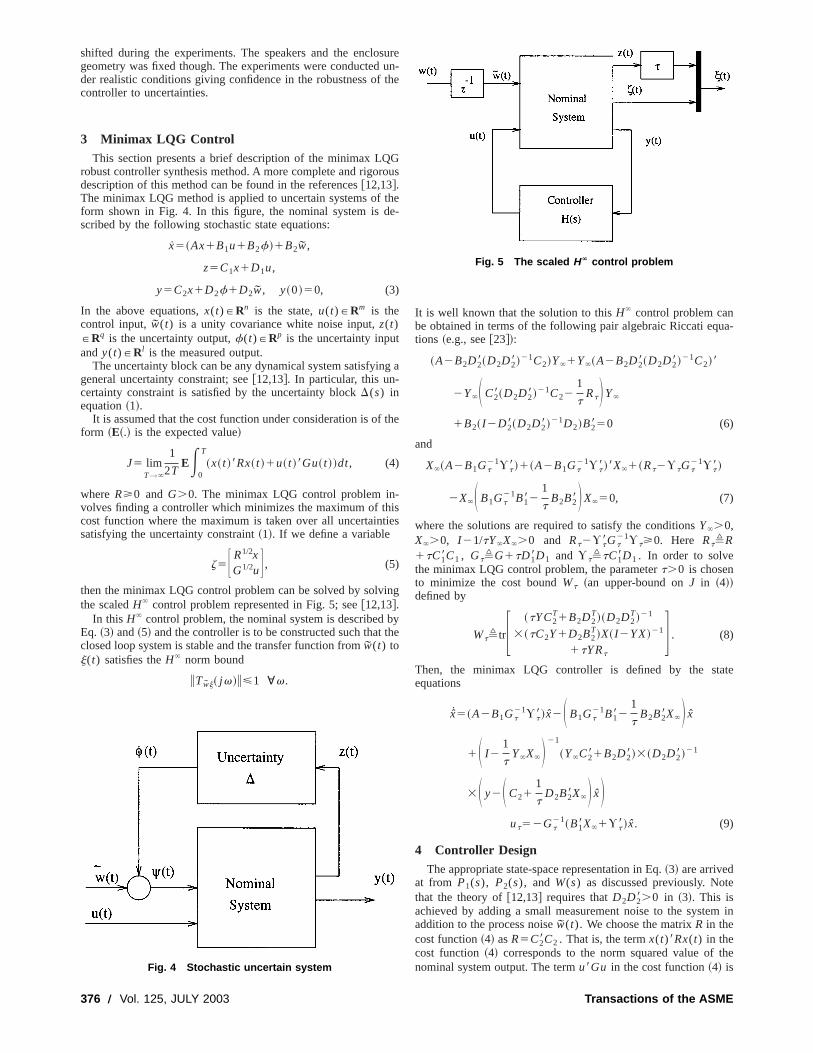
shifted during the experiments. The speakers and the enclosuregeometry was fixed though. The experiments were conducted un-der realistic conditions giving confidence in the robustness of thecontroller to uncertainties.

3 Minimax LQG ControlThis section presents a brief description of the minimax LQG

robust controller synthesis method. A more complete and rigorousdescription of this method can be found in the references@12,13#.The minimax LQG method is applied to uncertain systems of theform shown in Fig. 4. In this figure, the nominal system is de-scribed by the following stochastic state equations:

x5~Ax1B1u1B2f!1B2w,

z5C1x1D1u,

y5C2x1D2f1D2w, y~0!50, (3)

In the above equations,x(t)PRn is the state,u(t)PRm is thecontrol input,w(t) is a unity covariance white noise input,z(t)PRq is the uncertainty output,f(t)PRp is the uncertainty inputandy(t)PRl is the measured output.

The uncertainty block can be any dynamical system satisfying ageneral uncertainty constraint; see@12,13#. In particular, this un-certainty constraint is satisfied by the uncertainty blockD(s) inequation~1!.

It is assumed that the cost function under consideration is of theform ~E~.! is the expected value!

J5 limT→`

1

2TEE

0

T

~x~ t !8Rx~ t !1u~ t !8Gu~ t !!dt, (4)

whereR>0 andG.0. The minimax LQG control problem in-volves finding a controller which minimizes the maximum of thiscost function where the maximum is taken over all uncertaintiessatisfying the uncertainty constraint~1!. If we define a variable

z5F R1/2xG1/2uG , (5)

then the minimax LQG control problem can be solved by solvingthe scaledH` control problem represented in Fig. 5; see@12,13#.

In this H` control problem, the nominal system is described byEq. ~3! and~5! and the controller is to be constructed such that theclosed loop system is stable and the transfer function fromw(t) toj(t) satisfies theH` norm bound

iTwj~ j v!i<1 ;v.

It is well known that the solution to thisH` control problem canbe obtained in terms of the following pair algebraic Riccati equa-tions ~e.g., see@23#!:

~A2B2D28~D2D28!21C2!Y`1Y`~A2B2D28~D2D28!21C2!8

2Y`S C28~D2D28!21C221

tRtDY`

1B2~ I 2D28~D2D28!21D2!B2850 (6)

and

X`~A2B1Gt21Yt8!1~A2B1Gt

21Yt8!8X`1~Rt2YtGt21Yt8!

2X`S B1Gt21B182

1

tB2B28DX`50, (7)

where the solutions are required to satisfy the conditionsY`.0,X`.0, I 21/tY`X`.0 and Rt2Yt8Gt

21Yt>0. Here Rt,R1tC18C1 , Gt,G1tD18D1 and Yt,tC18D1 . In order to solvethe minimax LQG control problem, the parametert.0 is chosento minimize the cost boundWt ~an upper-bound onJ in ~4!!defined by

Wt,trF ~tYC2T1B2D2

T!~D2D2T!21

3~tC2Y1D2B2T!X~ I 2YX!21

1tYRt

G . (8)

Then, the minimax LQG controller is defined by the stateequations

x5~A2B1Gt21Yt8!x2S B1Gt

21B1821

tB2B28X`D x

1S I 21

tY`X`D 21

~Y`C281B2D28!3~D2D28!21

3S y2S C211

tD2B28X`D xD

ut52Gt21~B18X`1Yt8!x. (9)

4 Controller DesignThe appropriate state-space representation in Eq.~3! are arrived

at from P1(s), P2(s), and W(s) as discussed previously. Notethat the theory of@12,13# requires thatD2D28.0 in ~3!. This isachieved by adding a small measurement noise to the system inaddition to the process noisew(t). We choose the matrixR in thecost function~4! asR5C28C2 . That is, the termx(t)8Rx(t) in thecost function~4! corresponds to the norm squared value of thenominal system output. The termu8Gu in the cost function~4! isFig. 4 Stochastic uncertain system

Fig. 5 The scaled H` control problem


treated as a design parameter affecting controller gain. However,in all cases it was found that settingG to the small value ofG51028 did not lead to excessive controller gains.

Note that with the above choice of plant model~3! and costfunction~4!, the nominal LQG problem essentially amounts to theproblem of minimizing the noise energy at the microphone posi-tion when the system is subject to a white noise disturbance en-tering the system through the control input channel.

The minimax LQG controller is synthesised by first choosingthe constantt.0 to minimize the quantityWt defined in Eq.~8!.With this value of the parametert, the controller is constructedaccording to the formula~9!. The order of this controller will bethe sum of the order of the nominal plant modelP(s) together

Fig. 6 Two dimensional duct feedback controller setup

Fig. 7 Experimental and identified disturbance speaker response

Fig. 8 Experimental and identified control speaker response


with the order of the weighting filterW(s). Typical order of con-trollers designed in this paper is around eighty. Such a high ordercontroller may lead to problems of numerical error and excessivecomputational load when implemented. Hence, the balanced con-troller reduction method described in Section 19.1.1 of@23# isapplied to reduce the controller order to around forty. It was foundthat with this level approximation, there was very little degrada-tion in the predicted closed loop performance.

5 Experimental Results

The reduced dimension controller designed in Section 4 wasimplemented on a dSPACE DS1103 system as shown in Fig. 6.The spectrum analyser is used to measure the closed loopfrequency response from the disturbance speaker input to themicrophone output. In order to implement each controller, itwas first discretized using the FOH method with a sample period

Fig. 9 Uncertainty bound „dashed-20 log 10 zW„ j v…z,solid-20 log 10 zP2„ j v…

ÀP2„ j v…zÕiP1„ j v…z…

Fig. 10 LQG minimax controller


of 0.531023 seconds. The resulting discrete time controllerwas then implemented on the dSPACE system with this sampleperiod.

5.1 Control of Low Frequency Modes. Experimental fre-quency response data was collected from 20–500 Hz. It is notpractical to fit a model over the entire frequency range. A 40thorder model was fitted in the 20–100 Hz frequency range. Figures7 and 8 show the experimental response and the identified re-sponse for the disturbance and control speakers, respectively.

From the figures it can be seen that even a 40th order model isunable to match the data exactly.

The uncertainty envelopeW(s) and the magnitude of the 40thorder transfer function, for the identified models in Figs. 7 and 8,derived using Yule-Walker method is shown in Fig. 9.

For the case under discussion the controller order is 80 andbalanced model reduction technique@23# was applied in order toobtain a 40th order approximation to the 80th order controller. Thedesigned controller is shown in Fig. 10.

Fig. 11 Nyquist plot of the loop-gain

Fig. 12 Simulated closed loop and open loop response


The predicted stability and robustness of the closed loop systemcan be seen by the Nyquist plot based on the final~reduced di-mension! controller transfer function and the measured planttransfer function dataP2( j v). This Nyquist plot is shown in Fig.11. The disturbance attenuation performance of the controller isillustrated in Fig. 12.

Figure 13 shows the resulting measured frequency response forthe open loop and closed loop system.

5.2 Control of Higher Frequency Modes. The experimen-tal results presented thus far were restricted to the lower frequencyrange of 20–100 Hz. In this section the minimax LQG control

method is used to demonstrate the controller performance between250–450 Hz. The identified and experimental responses areshown in Figs. 14 and 15. The choice of uncertainty envelope andthe experimental closed loop and open loop performance is shownin Figs. 16 and 17, respectively. The frequency response outsideof the range shown in these figures remained unchanged. There isa clear improvement in the damping of the resonant peaks in thefrequency range of interest.

5.3 Proper Choice of the Uncertainty Model. It is shownin Section 3 that the minimax LQG control problem is equivalentto the minimization of theH` norm of the closed-loop transfer

Fig. 13 Experimental closed loop and open loop response

Fig. 14 Experimental and identified control speaker response


function between the noise inputw(t) and outputj(t) as definedin Fig. 5. The outputj(t) consists of two terms, one of them is theuncertainty outputz(t) which is also known as performance out-put. To minimize theH` norm the controller will attempt to keepthe outputz(t) small. From this we realize thatW(s) ~whoseoutput isz(t)) should be kept small for high authority control. Inobtaining models for acoustic enclosures it is seen that the mod-elling error is the largest at deep nulls. A proper placement of

actuators and sensors can be used to get rid of deep nulls. In otherwords optimal actuator-sensor placement methods should usemodelling error as a measure of optimality.

The influence of the choice ofW(s) on the controller can beused to shape the controller. For example, the frequency bandwhere uW(v)u is large, the controller gain will be low. In theclosed-loop response in Fig. 13 it can be seen that there is anincrease in the gain near the deep null around 70 Hz. This is due

Fig. 15 Experimental and identified disturbance speaker response




to the extreme difficulty in finding a good match between theidentified model and the experimental data. To shape the closedloop response at 70 Hz the choice of frequency weighting functionW(s) can be such that it is very conservative above 70 Hz asshown in Fig. 18. The conservative choice of the envelope atfrequencies greater than 70 Hz ensures that the controller doesn’thave high gain in that region. The experimental response of thecontroller designed with this method is shown in Fig. 19. Fromthe figure it’s clear that a proper selection of the weighting func-tion helps in shaping the closed loop response.

6 Conclusions

This paper successfully demonstrates that feedback control canbe applied to very high order acoustical systems for active noisecontrol. Due to the practical difficulty in implementing very highorder controllers it is essential that a small frequency band beselected for noise attenuation. The chosen minimax LQG controlmethod gives the flexibility to choose the frequency weightingfunction W(s) such that the controller targets a specified fre-quency band. Overall the experimental results in this work are

Fig. 17 Experimental open loop and closed loop response




very impressive and further work in the selection of actuator-sensor placement~to obtain a tighter fit between the model anddata! and a choice of frequency weighting function can improvethe results significantly.

References@1# Elliott, S. J., 1999, ‘‘Down with Noise,’’ IEEE Spectrum, June, pp. 54–61.@2# Hu, J.-S., Yu, S.-H., and Hsieh, C.-S., 1998, ‘‘Application of Model-Matching

Techniques to Feedforward Active Noise Control Design,’’ IEEE Trans. Con-trol Syst. Technol.,6~1!, pp. 33–42.

@3# Omoto, A., and Elliott, S. J., 1999, ‘‘The Effect of Structured Uncertainty inthe Acoustic Plant on Multichannel Feedforward Control Systems,’’ IEEETrans. Speech Audio Process.,7~2!, pp. 204–212.

@4# Pota, H. R., and Kelkar, A. G., 2001, ‘‘Modelling and Control of AcousticDucts,’’ ASME J. Vibr. Acoust.,123~1!, pp. 2–10.

@5# Kelkar, A. G., and Pota, H. R., 2000, ‘‘Robust Broadband Control of AcousticDuct,’’ Proceedings of the 39th IEEE Conference on Decision and Control,Sydney, Australia, pp. 4485–4490.

@6# Hong, J., Akers, J. C., Venugopal, R., Lee, M.-N., Sparks, A. G., Washabaugh,P. D., and Bernstein, D. S., 1996, ‘‘Modeling, Identification, and FeedbackControl of Noise in an Acoustic Duct,’’ IEEE Trans. Control Syst. Technol.,4~3!, pp. 283–291.

@7# Clark, R. L., and Cole, D. G., 1995, ‘‘Active Damping of Enclosed SoundFields Through Direct Rate Feedback Control,’’ J. Acoust. Soc. Am.,97~3!, pp.1710–1716.

@8# Erwin, R. S., and Bernstein, D. S., 1997, ‘‘Discrete-timeH2 /H` Control of anAcoustic Duct: Delta-domain Design and Experimental Results,’’Conferenceon Decision and Control, IEEE, San Deigo, CA, pp. 281–282.

@9# Petersen, I. R., and Pota, H. R., 2000, ‘‘Minimax LQG Optimal Control of anExperimental Acoustic Duct,’’IEE Control 2000 Conference, Cambridge, UK.

@10# Petersen, I. R., 2001, ‘‘Multivariable Control of Noise in an Acoustic Duct,’’Proceedings of the European Control Conference ECC2001, Porto, Portugal.

@11# Pota, H. R., and Kelkar, A. G., 2001, ‘‘On Perfect Acoustic Noise CancellingControl,’’ Control and Intelligent Systems,29~2!, pp. 48–54.

@12# Petersen, I. R., Ugrinovski, V., and Savkin, A. V., 2000,Robust Control Designusing H` Methods, Springer-Verlag, London.

@13# Ugrinovskii, V. A., and Petersen, I. R., 1998, ‘‘Time-averaged Robust Controlof Stochastic Partially Observed Uncertain Systems,’’Proceedings of the IEEEConference on Decision and Control, IEEE, Tampa, FL.

@14# Fang, B., Kelkar, A. G., and Joshi, S. M., 2002, ‘‘Modelling and Control ofAcoustic-Structure Interaction in 3-D Enclosures,’’IEEE 2002 Conference onDecision and Control, Las Vegas, Nevada.

@15# Ding, W. P., and Chen, H. L., 2001, ‘‘A Symmetrical Finite Element Model forStructure-Acoustic Coupling of an Elastic, Thin-Walled Cavity,’’ J. SoundVib., 243~3!, pp. 547–559.

@16# Marburg, S., Beer, H.-J., Gier, J., Hardtke, H.-J., Rennert, R., and Perret, F.,2002, ‘‘Experimental Verification of Structural-Acoustic Modelling and De-sign Optimization,’’ J. Sound Vib.,252~4!, pp. 591–615.

@17# Banks, H. T., Brown, D. E., Smith, R. C., Metcalf, V. L., Wang, Y., and Silcox,R. J., 1994, ‘‘Noise Control in a 3-D Structural Acoustic System: Numericaland Experimental Implementation of a PDE-Based Methodology,’’IEEE Pro-ceedings of the 33rd Conference on Decision and Control, Lake Buena Vista,FL, pp. 305–310.

@18# Nelson, P. A., and Elliott, S. J., 1992,Active Control of Sound, AcademicPress, London.

@19# Elliott, S., 2001,Signal Processing for Active Control, Academic Press, Syd-ney.

@20# McKelvey, T., Akcay, H., and Ljung, L., 1996, ‘‘Subspace-based MultivariableSystem Identification from Frequency Response Data,’’ IEEE Trans. Autom.Control,41~7!, pp. 960–979.

@21# Friedlander, B., and Porat, B., 1984, ‘‘The Modified Yule-Walker Method ofARMA Spectral Estimation,’’ IEEE Trans. Aerosp. Electron. Syst.,20~2!, pp.158–173.

@22# Petersen, I. R., Pota, H. R., and Jahromi, M. R. S., 2002, ‘‘System Identifica-tion, Uncertainty Modelling and Actuator Placement in the Robust Control ofan Acoustic Duct,’’Proceedings of the Conference on Information, Decision,and Control, Adelaide, Australia.

@23# Zhou, K., Doyle, J. C., and Glover, K., 1996,Robust and Optimal Control,Prentice Hall, NJ.

Fig. 19 Experimental closed loop and open loop response


Rifat Sipahi

Nejat Olgac*

Mechanical Engineering Department,University of Connecticut,

Storrs, CT 06269

Active Vibration Suppression WithTime Delayed FeedbackVarious active vibration suppression techniques, which use feedback control, are imple-mented on the structures. In real application, time delay can not be avoided especially inthe feedback line of the actively controlled systems. The effects of the delay have to bethoroughly understood from the perspective of system stability and the performance of thecontrolled system. Often used control laws are developed without taking the delay intoaccount. They fulfill the design requirements when free of delay. As unavoidable delayappears, however, the performance of the control changes. This work addresses the sta-bility analysis of such dynamics as the control law remains unchanged but carries theeffect of feedback time-delay, which can be varied. For this stability analysis along thedelay axis, we follow up a recent methodology of the authors, the Direct Method (DM),which offers a unique and unprecedented treatment of a general class of linear timeinvariant time delayed systems (LTI-TDS). We discuss the underlying features and thehighlights of the method briefly. Over an example vibration suppression setting we declarethe stability intervals of the dynamics in time delay space using the DM. Having assessedthe stability, we then look at the frequency response characteristics of the system asperformance indications.@DOI: 10.1115/1.1569942#

1 IntroductionActive vibration suppression has long been implemented on

structures under oscillatory excitations in various ways@1,3,4#. Ingeneral, a partial or full state feedback control law is utilized inorder to achieve good suppression performance. Most generallythis is represented as a multi input-multi output~MIMO ! statespace form of:

x5Ax1Bu1F (1)

whereu is the full state feedback, given by:

u5Kx (2)

⇒ x5~A1B…x1F (3)

Herex(n31) is the state vector,A(n3n), B(n3m) are the system andthe control matrices, respectively,K (m3n) is the full state feedbackgain matrix,F(n31) is the excitation~disturbance! force acting onthe structure, andB5BK . Utilizing the full state feedback law Eq.~2!, vibration suppression performance can easily be improvedwithin the frequency range of the excitation forcesF.

It is very well known, however, that the control systems arecommonly subject to time delay, which converts Eq.~3! into aretarded time delayed system~RTDS! which is given as:

x5Ax1Bx~ t2t!1F tPR1 (4)

wheret is the time delay influencing the system dynamics.It is critical to understand that the time delay may appear due to

the inherent nature of the core dynamics@5–6# as well as thefeedback control@1–2,7–8#. Regardless of the reason of the delayin the dynamics

~a! the underlying mathematics~i.e., retarded time delayed sys-tems! remains the same. The novel treatment presented in this textis applied to vibration suppression problems, although it is genericenough to be considered for a wide variety of TDS’s.

~b! it may deteriorate the quality of vibration suppression andin the worst case it can even drive the dynamics into instability.

In short, the dynamics of a typical active vibration suppressionsystem needs to be carefully evaluated with special considerationof delay. The unforced dynamics of the system is:

x5Ax1Bx~ t2t! tPR1 (5)

and it has to be studied from the stability perspective. Equation~5!represents a widely utilized class of linear time invariant retardedtime delayed systems~LTI-RTDS!. This general class of systemshas been extensively investigated for over four decades@9–19#.The deployment of a recently developed Direct Method~DM!@2,22# which yields unique observations on the system stabilityand the ensuing vibration suppression performance of Eq.~4!form the main theme of the present text.

Until the Direct Method~DM! the stability posture of the LTI-TDS along the axis of time delay was not completely resolved.That is, acompleteset of values of delay which cause stable orunstable behavior were not available through a systematic andpractical methodology.@18# gives an extensive review of the state-of-the art in this venue, including the techniques developed up to2001. Most of the later methods convert the LTI-TDS into a dis-tributed time delay equation via an integral transformation as ex-plained in@20#. They indicate that there are some additional dy-namics appearing due to this transformation. Consequently, thenew dynamics invites additional characteristic roots, which im-pose adverse restrictions on the range of time delay. Other meth-ods, which are mainly based on various Lyapunov-Krasovskifunctional @18,20–21#, bring conservative solutions for the stableregions of time delay. A recent publication@19# compares fivedifferent approaches~all developed in the 90s! based on Lyapunovand LMI ~linear matrix inequality! techniques. It is rather intrigu-ing to observe that even the best stability margin that these meth-ods can provide is more than 50% conservative with respect to thetrue margin~which is detected by following a tedious Nyquistmethod!. In contrast, the DM@22# coincides with the Nyquistresults precisely, furthermore it is numerically very efficient.These features make the Direct Method, extremely compelling.

Another shortfall of the existing methods is that, they all startwith a stabledynamics for nondelayed~i.e., delay50! case. Andthey try to assess the first positive delay value, which brings in-stability. This value forms the so-called, ‘‘delay margin’’ of thesystem and the stability analysis stops at that point. However, asrealized by many investigators@23–26#, there can be more than

*Author of correspondence. E-mail: [email protected] by the Technical Committee on Vibration and Sound for publication

in the JOURNAL OF VIBRATION AND ACOUSTICS. Manuscript received Feb. 2002;Revised Nov. 2002. Associate Editor: J. Wickert.


one such stable pocket in delay domain. This knowledge is ex-tremely important, as one can imagine. If there are so called, thesecondary stability pockets one may opt to operate within one ofthese, still performing a stable control despite the larger time de-lay in the picture. No existing methodology, however, could offera procedure to detect these additional pockets. The Direct Method~DM! @22# suggests a unique construct ultimately yielding an ex-plicit function of delay, which declares completely the stabilitypockets. The end results clearly offer much stronger revelationsthan simply stating the stability margin. The method is the first ofits kind as it handles the generaln-dimensional LTI-RTDS~withcommensurate time delays! and uncovers its unique properties.Some of these properties are realized in@23# for scalar dynamics(n51), however the approach therein is quite restrictive to imple-ment on a general LTI-RTDS~i.e. n.1). For these reasons, theDirect Method is unique in the dynamic systems and controlscommunity, opening number of new directions for future research.We wish to summarize the strong features of the Direct Methodhere to better prepare the reader:

i. It does not have to start with a stable system for zero delay.ii. It is exact, i.e. the limits of the stability pockets are precise.

They are not conservative results, which is a concern for thepeer methodologies@9–10,18–21,23#.

iii. All stable pockets are declared exclusively, in one explicitfunction of time delay.

In what follows we briefly review the procedure suggested bythe DM leaving the details to@22#. The system in Eq.~5! has atranscendental characteristic equation:

CE~s,t!5det~sI2A2Be2ts!5(j 50

n

aj~s!e2 j ts50 with t.0

(6)

whereaj (s)’s are polynomials in ‘‘s’’ of degreen2 j for retardedtime delayed dynamics. ClearlyCE(s,t) has infinitely many fi-nite characteristic roots, which move on the complex plane astvaries. As indicated by the feature~i! above, this system could beunstable when free of delay. The number of unstable roots for thiscase, can be determined using, for instance, Routh’s array. As amatter of fact, these roots are nothing but then eigenvalues ofA1B and they can also be calculated numerically to display thenatural response characteristics of the system, fort50. The inter-esting outcome of this work could be that, if a system is unstablefor t50, it may return to stability ast increases. This would be abeneficial effect of the time delay on the dynamics.

As t increases thesen characteristic roots start moving, alongwith infinitely many other roots~because of the transcendentalityof Eq. ~6!!, what we call the ‘‘secondary’’ roots. These secondaryroots are dormant, stable roots fort50 ~i.e. they are all in theform of 2`7ai ~a finite and real!, and they do not contribute tothe natural response of the system!. But they play a very criticalrole whent.0, because they creep into the finite domain andbecome influential. They may even destroy the stability of thedynamics.

Obviously for certain values oft.0 some of the infinitelymany characteristic roots cross the imaginary axis~excludingthose dynamics that are stable independent of time delay!, causinga transition from stable to unstable half of the complex plane~orvice versa!. These crossing frequencies (7v i ) and thet valuesgenerating them must all be detected exhaustively for a completestability analysis.

At this point, we state two very critical propositions from@22#,which eventually yield the three conclusions marked i, ii, iiiabove. We will recite them here for clarity, leaving their proofsto @2,22#.

Proposition I: The time delayed system in Eq.~5! can haveonly a finite number of imaginary characteristic roots~call these7vcki , k51, . . .m), for all values oftPR1. Note that, thesubscript ‘c’ refers to the ‘crossing’ of the roots over the imagi-

nary axis. The correspondingt values are$tk,%, k51, . . .m,,50, . . .` which are distributed periodically~by 2p/vck.! Thisproposition implies that the infinitely many characteristic roots ofEq. ~6! can only move across the imaginary axis through thesem‘pinholes’ (vcki ,k51, . . .m).

Proposition II : As t transits through one of the$tk,%, k51, . . .m, ,50, . . .` values, the respective root can passthrough the pinholevcki only in one direction. That is, the roottendency~RT! which is defined as

RTuv5vckt5tk,

5sgnFReS ds

dtUs5vckit5tk,

D G k51, . . .m,50, . . .` (7)

is invariant of the particular delayt5tk1p2p/vck , p50, . . .` which generates the crossingvcki .

What this proposition conceptually implies is that all of thempinholes for the possible passages of the characteristic rootsthrough the imaginary axis are guarded by ‘‘one-way checkvalves.’’

In Section 2, we introduce the steps of DM, and two proposi-tions, as well as the novel stability analysis, the ‘‘Direct Method,’’are followed by an application on a realistic vibration controlproblem, in Section 3.

2 The Direct MethodFor completeness of the treatment, we wish to review the Direct

Method~DM! briefly here. The stability assessment of the system~5! is needed in the domain oft ~the only free parameter in~5!!.DM starts with detecting all the crossing frequenciesvck (k51, . . .m) as described in Proposition I and the correspondingtime delays

tk,5tk012p

vck, ,50, . . .` (8)

which create these crossings.The following structured steps are performed next for the DM

stability analysis:~1! All imaginary roots and generatort’s are assembled as:

@vck ,$tk,%#, k51, . . .m, ,50, . . .`

~2! The set of common root tendencies RT at each one of thesem crossing frequencies are evaluated,RTuvck

. As per PropositionII, this is invariant of the value of$tk,%, k51, . . .m.

~3! All $tk,%, k51, . . .m, ,50, . . .` are tabulated in an ar-ray, in ascending order, along with thevck’s andRTuvck

’s.~4! The number of unstable roots (NU) is determined fort50

~non-delayed case!. Call this numberNU(0).~5! Take the nexttk, in ascending order and checkRTuvck

. It isobvious that, forRT511, NU increases by 2, and forRT521, NU decreases by 2. Repeat this step for the followingt’suntil the particular target value of delayt is reached.

~6! Identify those regions int whereNU(t)50 as ‘stable’ andothers as ‘unstable’. Also, state theNU(t) as the number of un-stable roots in this interval oft.

This procedure, indeed, lends itself to a novel explicit expres-sion of NU(t), owing to the Propositions I and II:

NU~t!5NU~0!1(k51

m

GS t2tk0

DtkD •U~t,tk0!•RTk (9)

whereNU(0) is the number of unstable roots whent50,U(t,tk0)5A step function int with the step taking place attk0


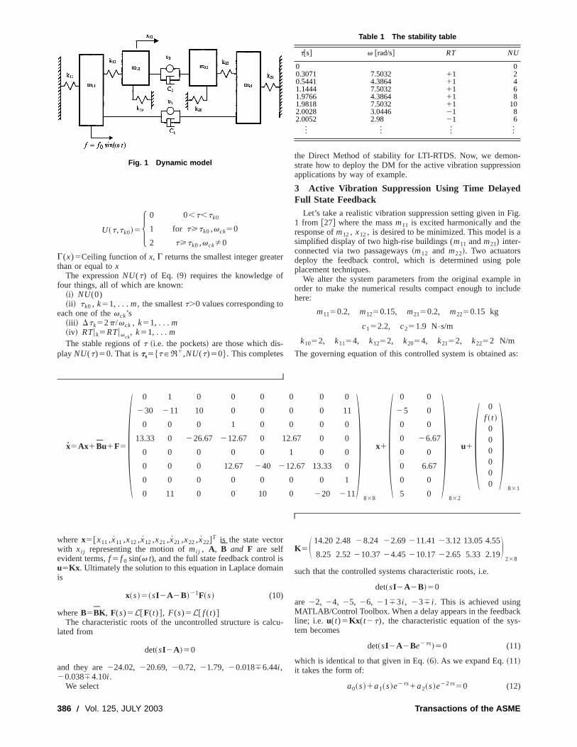
U~t,tk0!5H 0 0,t,tk0

1 for t>tk0 ,vck50

2 t>tk0 ,vckÞ0

G(x)5Ceiling function ofx, G returns the smallest integer greaterthan or equal tox

The expressionNU(t) of Eq. ~9! requires the knowledge offour things, all of which are known:

~i! NU(0)~ii ! tk0 , k51, . . .m, the smallestt.0 values corresponding to

each one of thevck’s~iii ! Dtk52p/vck , k51, . . .m~iv! RTuk5RTuvck

, k51, . . .mThe stable regions oft ~i.e. the pockets! are those which dis-

play NU(t)50. That ists5$tPR1,NU(t)50%. This completes

the Direct Method of stability for LTI-RTDS. Now, we demon-strate how to deploy the DM for the active vibration suppressionapplications by way of example.

3 Active Vibration Suppression Using Time DelayedFull State Feedback

Let’s take a realistic vibration suppression setting given in Fig.1 from @27# where the massm11 is excited harmonically and theresponse ofm12, x12, is desired to be minimized. This model is asimplified display of two high-rise buildings (m11 andm21) inter-connected via two passageways~m12 and m22!. Two actuatorsdeploy the feedback control, which is determined using poleplacement techniques.

We alter the system parameters from the original example inorder to make the numerical results compact enough to includehere:

m1150.2, m1250.15, m2150.2, m2250.15 kg

c152.2, c251.9 N•s/m

k1052, k1154, k1252, k2054, k2152, k2252 N/m

The governing equation of this controlled system is obtained as:

x5Ax1Bu1F510 1 0 0 0 0 0 0

230 211 10 0 0 0 0 11

0 0 0 1 0 0 0 0

13.33 0 226.67 212.67 0 12.67 0 0

0 0 0 0 0 1 0 0

0 0 0 12.67 240 212.67 13.33 0

0 0 0 0 0 0 0 1

0 11 0 0 10 0 220 211

2838

x110 0

25 0

0 0

0 26.67

0 0

0 6.67

0 0

5 0

2832

u1S 0f ~ t !000000

D831

where x5@x11,x11,x12,x12,x21,x21,x22,x22#T is the state vector

with xi j representing the motion ofmi j , A, B and F are selfevident terms,f 5 f 0 sin(v t), and the full state feedback control isu5Kx . Ultimately the solution to this equation in Laplace domainis

x~s!5~sI2A2B!21F~s! (10)

whereB5BK , F(s)5L@F(t)#, F(s)5L@ f (t)#The characteristic roots of the uncontrolled structure is calcu-

lated from

det~sI2A!50

and they are224.02, 220.69, 20.72, 21.79, 20.01876.44i ,20.03874.10i .

We select

K5S 14.20 2.48 28.24 22.69 211.4123.12 13.05 4.55

8.25 2.52210.3724.45 210.1722.65 5.33 2.19D238

such that the controlled systems characteristic roots, i.e.

det~sI2A2B!50

are 22, 24, 25, 26, 2173i , 237 i . This is achieved usingMATLAB/Control Toolbox. When a delay appears in the feedbackline; i.e. u(t)5Kx (t2t), the characteristic equation of the sys-tem becomes

det~sI2A2Be2ts!50 (11)

which is identical to that given in Eq.~6!. As we expand Eq.~11!it takes the form of:

a0~s!1a1~s!e2ts1a2~s!e22ts50 (12)

Fig. 1 Dynamic model

Table 1 The stability table

t@s# v @rad/s# RT NU

0 00.3071 7.5032 11 20.5441 4.3864 11 41.1444 7.5032 11 61.9766 4.3864 11 81.9818 7.5032 11 102.0028 3.0446 21 82.0052 2.98 21 6

] ] ] ]


where ap(s) is a polynomial ins of degree 82p, p50, 1, 2.Notice that the largest commensurate delay is 2t in Eq. ~12! be-cause of the specific formation ofA andB matrices in this case.The stability analysis follows as described in Section 2.

All imaginary roots are calculated using the methodology pre-sented in@22# and they are tabulated along with the correspondingdelays and root tendencies~Proposition II! below.

H vc154.3864vc257.5032vc353.0446vc452.98

J → from ~8!5t1k50.5441

2pp

vc1

t2k50.30712pp

vc2

t3k52.00312pp

vc3

t4k52.00512pp

vc4

6→H RTu1511

RTu2511RTu3521RTu4521

J p50, . . .` (13)

That is, only 4 sets oftk,’s ~each with dimension of infinity!cause the roots pass through the pinholes ofvc1 , vc2 , vc3 , vc4in the direction given by root tendencies~for 11 from stable tounstable complex plane, and for21 vice versa!.

Continuing the listings of Eq.~13! one can simply form theTable 1, which we call the ‘‘stability table’’, in ascending order oftk, , k51, . . .m, 50, . . .`.

The correspondingNU(t) variation is like in Fig. 2. The sta-bility posture of the system is clear: it’s stable only for the timedelay 0,t,307 ms. Afterwards it never returns to stability. Whatthis implies in practice is that the delay on the feedback can onlybe within this range for stability. Beyond 307 ms, the given feed-back structure renders instability by enforcing unstable right-hand-side roots numbered byNU(t), as per Fig 2. A numericalsimulation study validates this finding as given in Fig. 3.

The end result of this effort is not the declaration of stable orunstable regions only, but also what happens to vibration suppres-sion in the stable regions when the delay exists. We taket5250ms ~knowing that it is harmless from stability perspective! andstudy the frequency response of the massm12 under f 0 sin(vt)harmonic excitation onm11. When Eq.~10! is solved forx12 itresults in:

x12~s!

F~s!5

216.78 s52186.52 s42887.89 s322930.75 s226516.5 s26155.36

s8125 s71272 s611724 s517172 s4120516 s3139520 s2146000 s124000(14)

Fig. 2 Number of unstable roots „NU… plot in t domain Fig. 3 Stability posture of the system

Fig. 4 Frequency responses of the dynamics


for non-delayed feedbacku5Kx (t) and

x12~s!

F~s!5

p0~s!1p1~s!e2ts1p2~s!e22ts

q0~s!1q1~s!e2ts1q2~s!e22ts(15)

for delayed feedbacku5Kx (t2t), wherepi(s), qi(s) are self-evident polynomials ofs.

The frequency response features of this system are given in Fig.4 for various cases. It is clear that the feedback controlled case Eq.~14! registers substantial improvement over the uncontrolled casefor v.2.7 rad/s. And the delayed case Eq.~15! is bringing furtherimprovement except in the frequency range of 7.1,v,8.1 rad/s.In any event, it offers much better vibration suppression than theuncontrolled~passive! case.

It is obvious that, Fig. 4 has meaning if and only if the systemis stable, which can only be assured using the Direct Methodpresented. Therefore the novel method plays a very critical role inthis operation.

4 ConclusionsA general active vibration suppression problem under delayed

feedback is investigated in this paper. It is well known that forsuch control systems, time delay plays a very important role onthe vibration suppression quality and more importantly on thestability of the system. In this phase, we need to fully understandthe stability picture of the dynamics under time delay influence,first. For this we deploy a unique procedure, the Direct Method.The method offers certain structured steps for the stability analysisand uncovers very interesting features of linear time invarianttime delayed systems~LTI-TDS!, which were not recognized ear-lier. Using the DM, one can determine the exact boundaries ofstable and unstable regions int ~time delay! domain. It is thenpossible to investigate the efficiency of a vibration suppressionapplication, maintaining the stability of the system under timedelay effects. And we include a comparison of controlled vibra-tion suppression for various frequency zones between the timedelayed and non-delayed cases.

References@1# Olgac, N., 1995, ‘‘Delayed Resonators as Active Dynamic Absorbers,’’ United

States Patent 5,431,261.@2# Olgac, N., Special Lecture at the 3rd IFAC Workshop on TDS 2001, http://

www.siue.edu/ifacdelay/@3# Seto, K., and Furuishi, Y., 1991, ‘‘A Study on Active Dynamic Absorber,’’

ASME Proceedings, Paper DE, Vol. 38, pp. 263–270.@4# Seto, K., and Yamashita, S., 1991, ‘‘Simultaneous Optimum Design Method

for Multiple Dynamic Absorbers to Control Multiple Resonance Peaks,’’ SAETransactions,100, pp. 1481–1489.

@5# Olgac, N., and Hosek, M., 1998, ‘‘A New Perspective and Analysis for Re-generative Machine Tool Chatter,’’ Int. J. Mach. Tools Manuf.,38~7!, pp. 783–798.

@6# Tlusty, J, 1985, ‘‘Machine Dynamics,’’ R. I. King, ed.,Handbook of HighSpeed Machining Technology, Chapman and Hall, New York.

@7# Olgac, N., and Holm-Hansen, B., 1994, ‘‘A Novel Active Vibration AbsorptionTechnique: Delayed Resonator,’’ J. Sound Vib.,176, pp. 93–104.

@8# Olgac, N., Elmali, H., Hosek, M., and Renzulli, M., 1997, ‘‘Active VibrationControl of Disturbed Systems Using Delayed Resonator with AccelerationFeedback,’’ ASME J. Dyn. Syst., Meas., Control,119, pp. 380–388.

@9# Chen, J., Gu, G., and Nett, C. N., 1994, ‘‘A New Method for Computing DelayMargins for Stability of Linear Delay Systems,’’ Syst. Control Lett.,26, pp.107–117.

@10# Chen, J., 1995, ‘‘On Computing the Maximal Delay Intervals for Stability ofLinear Delay Systems,’’ IEEE Trans. Autom. Control,40„6…, pp. 1087–1092.

@11# Hale, J. K., and Verduyn Lunel, S. M., 2001, ‘‘Effects of Small Delays onStability and Control,’’ Operator Theory; Advances and Applications,122, pp.275–301.

@12# Hale, J. K., and Verduyn Lunel, S. M., 2001, ‘‘Strong Stabilization of NeutralFunctional Differential Equations,’’ IMA J. Math. Control Inform.,19, pp.1–19.

@13# Hale, J. K., and Verduyn Lunel, S. M., 1993,Introduction to Functional Dif-ferential Equations, Springer-Verlag.

@14# Hale, J. K., Infante, E. F., and Tsen, F.-S. P., 1985, ‘‘Stability in Linear DelayEquations,’’ J. Math. Anal. Appl.,105, pp. 533–555.

@15# Hertz, D., Jury, E. I., and Zeheb, E., 1984, ‘‘Simplified Analytic Stability Testfor Systems with Commensurate Time Delays,’’ IEE Proc.,131~1!, Pt~D!, pp.52–56.

@16# Jalili, N., and Olgac, N., 1999, ‘‘Multiple Delayed Resonator Vibration Ab-sorber for MDOF Mechanical Structures,’’ J. Sound Vib.,223~4!, pp. 567–585.

@17# Kolmanovski, V. B., and Nosov, V. R., 1986,Stability of Functional Differen-tial Equations, Academic Press, London, Great Britain.

@18# Niculescu, S-I., 2001,Delay Effects on Stability, Springer-Verlag.@19# Zhang, J., Knospe, C. R., and Tsiotras, P., 2001, ‘‘Stability of Time-delay

Systems: Equivalence Between Lyapunov and Scaled Small-gain Conditions,’’IEEE Trans. Autom. Control,46~3!, pp. 482–486.

@20# Gu, K., and Niculescu, S.-I., 2000, ‘‘Additional Dynamics in TransformedTime-Delay Systems,’’ IEEE Trans. Autom. Control,45~3!, pp. 572–575.

@21# Park, P., 1999, ‘‘A Delay-Dependent Stability Criterion for Systems with Un-certain Time-Invariant Delays,’’ IEEE Trans. Autom. Control,44, pp. 876–877.

@22# Olgac, N., and Sipahi, R., 2002, ‘‘An Exact Method for the Stability Analysisof Time Delayed LTI Systems,’’ IEEE Trans. Autom. Control,47~5!, pp. 793–797.

@23# Cooke, K. L., and van den Driessche, P., 1986, ‘‘On Zeroes of Some Transcen-dental Equations,’’ Funkcialaj Ekvacioj,29, pp. 77–90.

@24# Thowsen, A., 1981, ‘‘The Routh-Hurwitz Method for Stability Determinationof Linear Differential-Difference Systems,’’ Int. J. Control,33~5!, pp. 991–995.

@25# Thowsen, A., 1981, ‘‘An Analytic Stability Test for a Class of Time-DelaySystems,’’ IEEE Trans. Autom. Control,26~3!, pp. 735–736.

@26# Thowsen, A., 1982, ‘‘Delay-independent Asymptotic Stability of Linear Sys-tems,’’ IEE Proc.,29, pp. 73–75.

@27# Seto, K., 1995, ‘‘Structural Modeling and Vibration Control.’’ Internal Report,Nihon University. Department of Mechanical Engineering, College of Scienceand Technology, Nihon University, 1-8-14 Kanda Surugadai Chiyoda-ku, To-kyo, 101-8308, Japan.


Gaetan Kerschene-mail: [email protected]

Jean-Claude Golinval

Vibrations & Identification des Structures,Department of Aerospace,Mechanics and Materials,

University of Liege,Chemin des Chevreuils 1 (B52),

B-4000 Liege, Belgium

Francois M. HemezEngineering Science & Applications Division,

ESA-WR, Mail Stop P946,Los Alamos National Laboratory,Los Alamos, New Mexico 87545


Bayesian Model Screening for theIdentification of NonlinearMechanical StructuresThe development of techniques for identification and updating of nonlinear mechanicalstructures has received increasing attention in recent years. In practical situations, thereis not necessarily a priori knowledge about the nonlinearity. This suggests the need forstrategies that allow inference of useful information from the data. The present studyproposes an algorithm based on a Bayesian inference approach for giving insight into theform of the nonlinearity. A family of parametric models is defined to represent the non-linear response of a system and the selection algorithm estimates the likelihood that eachmember of the family is appropriate. The (unknown) probability density function of thefamily of models is explored using a simple variant of the Markov Chain Monte Carlosampling technique. This technique offers the advantage that the nature of the underlyingstatistical distribution need not be assumed a priori. Enough samples are drawn to guar-antee that the empirical distribution approximates the true but unknown distribution tothe desired level of accuracy. It provides an indication of which models are the mostappropriate to represent the nonlinearity and their respective goodness-of-fit to the data.The methodology is illustrated using two examples, one of which comes from experimentaldata. @DOI: 10.1115/1.1569947#

1 IntroductionThe importance of diagnosing, identifying and modelling non-

linearity has been recognized for a long time, e.g., for the designof shock absorbers and engine mounts. The identification of non-linear systems began in 1979 with the introduction of the restoringforce surface~RFS! method by Masri and Caughey@1#. Anequivalent method, referred to as force-state mapping, was pro-posed independently by Crawley, Aubert and O’Donnel@2,3#.Since then, numerous methods were proposed. It is not our inten-tion to review all the methods available but rather to cite the mostpopular techniques that have been considered during the lasttwenty years.

The first application of the Hilbert transform was made in thefrequency domain@4#. The time-domain Hilbert transform wasalso utilized to solve an inverse problem@5,6#. The use of theVolterra series in the field of structural dynamics began in the late1980s@7#. NARMAX models consist of polynomials that includevarious linear and nonlinear terms combining the inputs, outputsand past errors and were introduced by Leontaritis and Billings@8,9#. Another area of signal processing that has gained impor-tance in studying nonlinear systems deals with higher-order spec-tra @10,11#. These are a natural extension of the ordinary linearspectral analysis. For a detailed description of all these tech-niques, the reader is referred to reference@12#.

The development of frequency response function-based ap-proaches has received increasing attention in recent years. Thereverse path technique has been proposed by Rice and Fitzpatrick@13# and applied to simulated and experimental data@14,15#. Theconditioned reverse path formulation@16# extends the applicationof the reverse path algorithm to systems characterized by nonlin-earities away from the location of the applied force. This methodexploits the spectral conditioning techniques introduced by Ben-dat @17#. A related series of papers by Adams and Allemang alsodevelop the frequency response function-based approaches@18,19#.

Finally, it is worth pointing out that there has also been a

growth in interest in a particular class of identification techniquesbased on a finite element model and referred to as finite elementmodel updating techniques@20–22#.

The problem of variable selection is one of the common issuesin the field of identification of nonlinear systems. The purpose isto model the relationship between the response variable of interestand a subset of predictor variables, possibly with interactions be-tween these latter variables. Generally speaking, there is uncer-tainty about which subset to use.

A possible means of determining which variables should beincluded in the model is through least-squares parameter estima-tion and the use of the significance factor@12#. Cumulative andmultiple coherence functions may also be used in conjunctionwith the conditioned reverse path formulation@23#. The presentstudy investigates an inference technique based on the Bayesiandefinition of probability—as opposed to the frequentist’s point-of-view—for identifying promising subsets of predictors@24–27#.While the frequentist interpretation defines probability strictly asthe number of occurrences of an event among a collective ofpossibilities, the Bayesian approach defines probability as the sub-jective opinion of the analyst or expert. To stress the differencebetween the two approaches, consider the simple question ‘‘Whatis the probability of life on the planet Mars?’’ Such questionmakes no sense in the frequentist framework because observationscan obviously not be obtained from a collective of planets similarto the planet Mars. Similarly and even though we might not al-ways be aware of it, many problems occur in structural dynamicsthat require probability to be defined in terms of our a prioriknowledge of the phenomenon studied. The identification of theform of a model is one such problem addressed in this work.

The procedure developed in this work exploits ‘‘priors’’—thatis, a probability structure that reflects the analyst’s a priori opinionabout the phenomenon investigated—on the variables of the re-gression model in order to give the list of all visited models to-gether with their relative posterior probabilities. Models are vis-ited according to their goodness-of-fit to the data, which, in theBayesian framework, represents the likelihood of predicting theobserved response. This implies that models well fitted to thedata—that is, more likely models—are visited more often. Themarginal probabilities of inclusion of single variables are also

Contributed by the Technical Committee on Vibration and Sound for publicationin the JOURNAL OF VIBRATION AND ACOUSTICS. Manuscript received May 2002;Revised January 2003. Associate Editor: M. I. Friswell.


computed. To avoid the overwhelming burden of calculating theposterior probabilities of all models, a Gibbs sampler is consid-ered to perform an efficient stochastic search of the model space.It is emphasized that the main difficulty of this inference problemis that the multi-dimensional probability density function~PDF! ofthe family of models must be sampled. However, this PDF isunknown, making random walk techniques such as the MarkovChain Monte Carlo~MCMC! sampling the only possible choice.Gibbs sampling has been proposed as a computationally attractivealternative to MCMC, yet, it can explore an unknown PDF@24,26#.

While the principle of Bayesian inference has previously beenapplied to various problems in structural dynamics~e.g., Refer-ences@28,29#!, no attempt has been made, to the best of the au-thors’ knowledge, to adapt the Bayes updating rule to the screen-ing of model form during nonlinear system identification. After abrief discussion of model fitting in Section 2, the Bayesian screen-ing algorithm for model selection is outlined in Section 3. Themethodology is illustrated using two examples. Section 4 dis-cusses a numerical simulation intended at demonstrating the over-all performance of the screening method. The second exampleinvolves experimental data sets collected during the EuropeanCOST-F3 program~Section 5!. The numerical predictability of theidentified model is finally assessed in Section 6.

2 Model FittingModel fitting generally refers to the calibration of model coef-

ficientsb given a sequence of points (tk ;yk) in the design space.It is assumed that a model is available:

y5M ~b;t ! (1)

wheret denotes the input variables,y denotes the output variablesandb denotes the model’s coefficients.

For clarity, the discussion will assume that the model form ispolynomial-like. Nevertheless, nothing prevents the Bayesianmodel screening proposed in Section 3 to be applied to otherfunctional forms. Fractional models could be considered, for ex-ample, to fit the poles and zeros of frequency response functions.Exponential models could be considered to represent the decay ofpropagating waves as a function of time or distance. Artificialneural networks are increasingly used in a variety of applicationsin structural dynamics because they can, depending on their form,approximate any non-linear function@30#.

Another notion that must be clarified before proceeding withthe discussion is the notion of ‘‘effect.’’ The model shown in Eq.~1! depends on inputst wheret does not necessarily refer to time.Functions of the input variablest can be defined that will bereferred to as effects and denoted byx in the following. Suchfunctions can assume any form, linear or non-linear. For example,the 2-input, 1-output nonlinear model:

y50.3t112.0 sin~ t2!21.5e2t1t2 (2)

can equivalently be defined through the three effectsx15t1 , x2

5sin(t2) andx35e2t1t2 as:

y50.3x112.0x221.5x3 (3)

While the input variablest1 and t2 might be independent, notethat the effectsx1 , x2 andx3 are neither independent nor uncor-related. The Bayesian model screening discussed in Section 3does not require the effects to be independent or uncorrelated.With the definition of effectsx that can be functions of the inputvariablest, the polynomial-like model can be simply representedas:

y5 (k51 . . .m

xkbk5xTb (4)

The commonly encountered method of fitting the coefficientsbis to define an objective function that represents the prediction

error and minimize it. The most straightforward choice is to adoptthe Euclidean norm of the prediction errorek5yk2xk

Tb:

J~b!5 (k51 . . .N

ekTek5eTe (5)

in which case the best, linear, unbiased estimator of the coeffi-cientsb is provided by:

b5~XTX!21XTy (6)

where the column-vectory collectsN observations and theN rowsby m columns matrixX evaluates them effects for each of theNobservations:

y5H y1

y2

]

yN

J ;X5F x1,1 x1,2 ¯ x1,m

x2,1 x2,2 ¯ x2,m

] ] � ]

xN,1 xN,2 ¯ xN,m

G (7)

Clearly, other objective functions yield different estimators. Thegeneralization of the objective function~5! is commonly referredto as the generalized least-squares~GLS! estimator@31#. Weight-ing matrices are introduced and a regularization term penalizessolutions too distant from the user-defined starting pointbo . Eqs.~8! and ~9! show the GLS objective and the corresponding GLSestimator, respectively:

J~b!5eTWee21e1~b2bo!TWbb

21~b2bo! (8)

b5~XTWee21X1Wbb

21!21XTWee21y (9)

In general, weighting matrices are chosen arbitrarily or basedon experience, for example, to weight the importance of someobservations more than others. When covariance matrices areused, the GLS estimator becomes similar to the Bayesian estima-tor. Rigorously speaking, other factors should appear in the defi-nition of the Bayesian objective function. Because these addi-tional factors are constant, however, the same estimator as the oneshown in Eq.~9! is obtained. An important benefit of Bayesianinference is that it provides a posterior estimate of the covariancematrix:

Wbb~posterior!5~Wbb

211XTWee21X!21 (10)

Correlation coefficients of the posterior covariance matrix~10!provide insight into the quality of the estimator. Reference@32#discusses a shock propagation application where significant pos-terior correlation is obtained between coefficients that have nophysical reason to be correlated. The authors conclude that theform of the model is inappropriate. They further demonstrate thatit is indeed the case when improved goodness-of-fit and posteriorcorrelation indicators are obtained with a different model.

With the exception of investigating the posterior correlation,however, no practical tool is available to select the appropriateform of a nonlinear model, which is the process we refer to amodel screening. Model form—for example, replacing a linearcontribution by a cubic stiffness—is usually selected based onexperience or empirical observation. Sometimes, several choicesseem equally likely and the analyst has to go through the pains-taking process of fitting each model and assessing their goodness-of-fit. Because it is based on the concept of goodness-of-fit, suchapproach leads to over-fitting.

Another subtle but important issue is to estimate the posteriorprobability of a particular model as opposed to simply relying onthe goodness-of-fit. By definition, the posterior probability is con-ditioned on the evidence available—that is, experimental observa-tions. Posterior probability and goodness-of-fit complement eachother because the former indicates if the analyst’s prior opinion ofthe form of the model is consistent with the evidence. In Section3, a practical tool is proposed for model screening based on theconcept of posterior probability.


3 Bayesian Model ScreeningIn the previous section, the state of the practice in model fitting

has been briefly overviewed. Polynomial models have been con-sidered for simplicity. It is emphasized that the Bayesian modelscreening technique proposed here applies to any model, no mat-ter which functional form it takes. Essentially, the only two gen-eral assumptions made are as follows. First, a modely5M (b;x) must be available. As previously mentioned, the effectsx can be linear or nonlinear functions of the input variablest.Second, an inference is available for calibrating the coefficientsb.The inference procedure is usually referred to as ‘‘best-fitting’’with polynomials and ‘‘training’’ with neural networks.

Model screening consists in identifying the most probable mod-els based on a family of models defined by the user and referencedata that the model’s predictions must reproduce with the highestpossible fidelity. It is emphasized that model screening does notnecessarily identify the best model but rather ranks potential mod-els according to their posterior probability of occurrence.

The procedure starts by, first, defining a family of models. Thisis achieved by defining various effectsxi and how these effectsare allowed to interact to form the population of potential models.Figure 1 illustrates the concept of a family of models by showingtwo effectsx1 and x2 that interact with each other. The model-forming rule illustrated in Fig. 1 is that linear and quadratic inter-actions are allowed between the effectsx1 andx2 . The horizontalplane represents the family of all potential models that must beexplored. The vertical dimension represents the likelihood that aparticular model is appropriate to represent the data. It is thisnotion of likelihood that will be employed to guide the search forthe most appropriate models. Figure 1 illustrates a hypotheticalsituation where the model shown with a star symbol,y5bo

1b1x21b2x121b3x2x1

2, is the maximum likelihood model.The second step of the procedure is to assign the prior prob-

ability of occurrence of each effectxi . The priors can reflectempirical observations, experience or the analyst’s knowledge ofthe system investigated. In the application discussed in Section 5,for example, no specific knowledge of the system can be used toguide a pertinent choice of priors. Probabilities of occurrence aretherefore set to a uniform 25% level for all effects.

The next step is to let the Bayesian screening method find themost appropriate models among all possible combinations of ef-fects. To identify the most probable models a measure ofgoodness-of-fit to the reference data must be defined. This can beassessed using a conventional root mean square~RMS! error be-tween data and predictions. Assuming Gaussian distributions, theRMS error becomes proportional to the likelihood functionL(yub) that estimates the likelihood that the model is appropriategiven the available data:

L~yub!5 (k51 . . .N

~yk2xkTb!2 (11)

Note that the likelihood function~11! is similar to Eq.~5! previ-ously discussed. Other functions can be used, in particular theBayesian objective~8!, as well as the many objective functionscommonly used in test-analysis correlation and model updating@33#.

Once the likelihood of a particular model has been estimated,the posterior probabilities of the model’s effects can be updatedaccording to the Bayes Theorem that states that the posterior prob-ability PDF(buy) is equal to the likelihood functionL(yub) mul-tiplied by the prior probability PDF(b) and divided by the prob-ability of the data PDF(y):

PDF~buy!5L~yub!PDF~b!

PDF~y!(12)

The probability of the observed data PDF(y) is generally keptconstant and omitted in the updating Eq.~12!. Because the proce-dure is iterative in nature, the Bayes update~12! is repeated and

posteriors of thenth iteration become the priors of the (n11)thiteration. All models visited are kept in memory and, once enoughsamples have been drawn, the probability of occurrence of eachmodel is estimated by the frequency of occurrence—that is, theratio between the number of times each model is visited and thetotal number of models visited. The iterative procedure is summa-rized in Fig. 2.

In summary, Bayesian model screening provides the probabili-ties of occurrence of the most appropriate members of a user-

Fig. 1 Concept of ‘‘family’’ of models

Fig. 2 Simplified flow chart of the Bayesian model screeningalgorithm


defined family of models, their goodness-of-fit indicators and theposterior probabilities PDF(buy) of effects involved in the mostlikely models.

To do so, however, the unknown posterior probability functionmust be sampled. The problem of exploring an unknown PDF issolved with the Markov Chain Monte Carlo algorithm. TheMCMC sampling is advantageous in this situation because it cansample any distribution, whether it is Gaussian or not. TheMCMC sampling can be viewed conceptually as an optimizationsolver that performs a random walk through the optimizationspace. This concept is illustrated in Fig. 3 where points in theoptimization space are sequentially visited. More appropriate so-lutions are guaranteed more frequent visits because the acceptancecriterion of a given solution is based on its likelihood function.

Each candidate point in the design space—here, the designspace is the horizontal plane of potential models illustrated inFigs. 1 and 3—is accepted or rejected based on its value of thelikelihood function~11! and a Chi-square test. This particular ac-ceptance criterion implies that inappropriate models have a smallchance of being accepted just like appropriate models have asmall chance of rejection. If rejected, a new point is randomlyselected in the neighborhood of the last accepted point. The se-quence of points accepted is stored to estimate, once the processhas been completed, the probability of occurrence of each model.

The sampling procedure used in this work is the Gibbs sam-pling, the simplest of the many variants of the MCMC algorithm.

The main difference between the two is that the Gibbs algorithmsamples one direction of the design space at a time, which makesfor simpler numerical implementation. Figure 4 illustrates the dif-ference between MCMC and Gibbs sampling. It pictures two ran-dom walks from the lower left corner (x50;y50) to the upperright corner (x51;y51). A constraint is enforced that preventsthe 30 points drawn in both sequences from being repeated andfrom moving backwards. Pentagram symbols show a sequence ofGibbs samples while hexagram symbols picture a realization ofthe MCMC chain. In the former case, the solution is advanced inone direction at a time whereas the MCMC chain randomly ad-vances the solution in the two dimensions simultaneously.

4 Numerical ApplicationThe first application presented is extremely simple and aims at

illustrating the overall performance of the model screening proce-dure. Consider an output variabley defined by the followinginput-output model:

y52 sin~2t !13 cos~ t !21.5 sin~3t !cos~2t ! (13)

where t is an input variable that varies from zero to fifty withincrements ofDt50.05. It is assumed that the model form shownin Eq. ~13! is unknown. Instead, observationsyk5y(kDt), for k50 . . . 100, are obtained and the problem consists in identifyingthe numerical model that best matches the observed data. It isemphasized that, in this numerical simulation, no actual experi-ment is performed. The continuous solution~13! is shown in Fig.5 with a solid line. The hexagram symbols represent the discretesamples assumed to be collected.

Next, consider a set of candidate predictors:

5x15sin~ t !x25cos~ t !x35sin~2t !x45cos~2t !x55sin~3t !x65cos~3t !

(14)

In addition to the six predictors of Eq.~14!, six other predictorslabeledx7 , x8 , x9 , x10, x11 andx12 are defined as random func-tions. It can be observed that, if the functional form of the outputvariabley were known, it could be written as:

y53x212x321.5x4x5 (15)

Fig. 3 Concept of random walk optimization

Fig. 4 Illustration of MCMC and Gibbs random walk samplingstrategies

Fig. 5 Simulated non-linear function „13…


Clearly,y does not depend on predictorsx1 , x6 , x7 , x8 , x9 , x10,x11 and x12. The objective of model screening is to identify themodel form~15!. Equivalently, it can be stated that the objectiveof model screening is to identify the linear effectsx2 , x3 and thelinear interaction effectx4x5 from all the potential combinationsdefined by the family of models considered.

The family of models defined for this illustration is composedof the linear models that include the twelve linear effectsxi andthe linear interaction models, defined as the previous models aug-mented with the 66 interaction effectsxixj . The total number ofdifferent effectsxi and xixj with twelve predictors is thereforeequal to 78. The total number of different models that can bedefined belonging to this family by combining the 78 effects is inexcess of 3.02 10123 models, a number that approaches the num-ber of atoms in the known Universe. Clearly, exploring such alarge number of combinations without focusing on the models ofhighest likelihood would not be feasible.

The procedure described in the foregoing section is applied tothe data using 50 samples dedicated to the initialization of theGibbs sampler and 100 samples for the computation. Initializingthe Markov chain is referred to as ‘‘burn-in’’ and guarantees thatthe remainder of the chain is not biased due to a particular choiceof starting point. The samples drawn during burn-in are disre-garded and only the 100 samples drawn during the optimizationitself are kept to estimate the final probability of occurrence ofeach model in the family. The top five models are listed in Table1. It can be observed that the best model in terms of posteriormodel probability is the actual model. The mean-square error forthe top five models is about 0.003%. This means that it is notnecessary to include other terms than the ones present in the bestmodel.

Figure 6 represents the marginal posterior probability of eacheffect being in a particular model. The prior probabilities—thatreflect the prior knowledge—are set to 25% for each linear effectxi ; 10% for the interaction effectsxixj if one of the parent effectxi or xj is selected in the model; and 1% only for the interactioneffectsxixj when neitherxi nor xj are considered in the model.

These uniform probabilities reflect the fact that little is knownabout the form of the model before starting the analysis. It can beobserved that effects 2, 3 and 43, namelyx2 , x3 and x4x5 , areassociated with a probability of 100% while the other effects maybe ignored because their posterior probabilities are reduced toinsignificant levels.

In conclusion, the Bayesian model screening clearly suggests amodel that includes the three effectsx2 , x3 andx4x5 . The iden-tified coefficients corresponding to these effects are equal to 2.99,2.02 and21.52, respectively, and they are in good agreement withthe actual coefficients shown in Eq.~15!. The algorithm is imple-mented as interpreted Matlab™ functions and it performs theanalysis in a few seconds of CPU time with a typical desktoppersonal computer.

5 Experimental ApplicationIn this Section, Bayesian model screening is applied to the

problem of identifying the form of a nonlinear model using real,experimental data. The analyzed data sets are chosen from thoseproposed by the VTT Technical Research Center of Finland withinthe framework of the European COST action F3 working groupon ‘‘Identification of Nonlinear Systems’’@34#.

The structure investigated consists of wire rope isolatorsmounted between the load mass and the base mass, as shown inFig. 7. The load mass acts like a free inertial mass. The motionand forces experienced by the isolators are measured. In particu-lar, the acceleration responsesx2 and x1b of the load mass andbottom plate, the applied forcef and the relative displacementx12between the top and bottom plates are measured. The excitationproduced by an electro-dynamic shaker corresponds to a whitenoise sequence, low-pass filtered at 400 Hertz. What makes thissystem interesting for identification is that the attenuation of thevibration across the interface is difficult to characterize becausethe mechanics of the isolators is unknown to a large extent. Sig-nificant nonlinear dynamics are expected due to the geometricalnonlinearity—pre-loading in the wire rope isolators changes withthe load mass.

Fig. 6 Marginal posterior probability of each effect included inthe family of models Fig. 7 Wire rope isolators

Table 1 Top five models and number of appearances

Model Effects Posterior Probability

1 x2 , x3 , x4x5 52.0%2 x2 , x3 , x4x5 , x10 3.0%3 x2 , x3 , x4x5 , x3x4 2.0%4 x2 , x3 , x4x5 , x2x10 2.0%5 x2 , x3 , x4x5 , x2x5 2.0%


Four excitation levels are considered ranging from 0.5 Volt upto 8.0 Volt. A nominal series of four tests are performed with aload mass of 2.2 kg. A fifth test is also carried out with the heavierload mass of 5.8 kg. Table 2 defines the testing matrix from whichdata sets have been collected.

Reference@35# discusses the identification of the VTT bench-mark structure using the RFS. The main idea behind the RFSmethod is briefly overviewed to explain the system identificationapproach and the reader is referred to Reference@35# for moredetails.

The derivation of the main equations of the RFS method startsby writing Newton’s second law for the load massm2 , whichyields:

m2x21 f NL~x22x1b ,x22 x1b!50 (16)

where f NL denotes the nonlinear internal force. Clearly, the forcef NL is unknown but it can be ascertained, as shown in Eq.~16!,that its value depends on the displacement and velocity of the loadmass relative to those of the bottom plate. Introducing the relativedisplacement,x125x22x1b , Eq. ~16! becomes:

f NL~x12,x12!52m2x1b2m2x12 (17)

Equation ~17! can be viewed as describing the response of aSDOF system subjected to a base acceleration. Because the accel-eration signals shown in the right-hand side of Eq.~17! are mea-sured and the mass is known, it is possible to compute the restor-ing force f NL at each instant from Eq.~17!.

The value of the restoring force is shown in Fig. 8 in the fourcases where the load mass is equal to 2.2 kg~Tests 1–4!. At lowexcitation level, the system’s behavior is predominantly linear be-cause the restoring force varies linearly with the displacement, ascan be observed for the 0.5 Volt and 2.0 Volt levels. As the exci-tation level is increased, a softening stiffness nonlinearity appears,as can be observed from the 4.0 Volt and 8.0 Volt levels.

The next step of the RFS method is to describe the restoringforce by means of a mathematical model. This is achieved throughmodel fitting such as described in Section 2. The generic form ofmodels sought is usually given by:

f ~x,x!5(i 50

m

(j 50

n

a i j xi x j (18)

To resolve the problem of order determination, which refers to theidentification of the most appropriate dimensionsm, n in Eq. ~18!,an over-determined system of linear equations is formed with theavailable restoring force data. The singular value decomposition isthen used to select the appropriate order. Reference@35# detailsthe identification procedure and shows that the final model in-cludes a linear stiffness term, a viscous damping term and a non-linear stiffness contribution:

f NL~x12,x12!5klx121cl x121knlux12uasign~x12! (19)

where the coefficientskl , cl , knl and a identified with the RFSmethod and singular value decomposition are listed in Table 3.These results are used in the remainder as the reference throughwhich the performance of the Bayesian model screening isassessed.

The final model features a mean square error~MSE! equal to2.11%, which indicates an excellent correlation to test data. TheMSE indicator is a normalized metric that measures the goodness-of-fit between model predictions and physical observations. It isdefined as:

MSE5100

Nsy2 (

k51 . . .N~yk2xk

Tb !2 (20)

where, to comply with notations introduced in Section 2,yk rep-resents the available restoring force data andsy is the standarddeviation of datayk . The vectorb collects the coefficientskl , clandknl , assuming that the exponenta is known and equal to 1.5,and the vectorxk collects the corresponding effects in Eq.~19!.

The exercise of identifying the most appropriate model form isnow repeated with the Bayesian model screening. First, three ef-fects are defined in agreement with Eq.~19!. They are the linearstiffness x12, linear damping x12 and nonlinear stiffnessux12uasign(x12). The corresponding coefficients are denoted bykl ,cl and knl , as before. Second, model-forming rules are definedwhich are that main effects and linear interactions between themain effects are allowed. This means that a total of six effectsleading to sixty two different model forms are allowed. Such com-binatorial complexity is trivial compared to the example discussedin Section 4. The complexity here stems from the fact that realdata sets are analyzed with all the risk of erroneous identificationcaused by ‘‘noisy’’ measurements and signal conditioning issues.

Because the exponenta is unknown, the Bayesian modelscreening is repeated for several assumed values ofa. The valuethat leads to the smallest MSE is retained. Repeating modelscreening could become CPU-time intensive if long MCMCchains are requested for each analysis. For this application, aninitial chain of length 50 is dedicated to burn-in and a chain oflength 300 is requested for the optimization. It has been verifiedthat requesting more samples does not improve the quality of thefinal results. Figure 9 shows the evolution of the MSE as a func-tion of the exponenta. The minimum value is obtained fora

Fig. 8 Estimation of the restoring force at the four levels 0.5Volt, 2.0 Volt, 4.0 Volt and 8.0 Volt

Table 2 Testing matrix of the VTT benchmark

Forcing Level Mass 1~2.2 kg! Mass 2~5.8 kg!

Level 1 ~0.5 volt! Test 1 —Level 2 ~2.0 volt! Test 2 —Level 3 ~4.0 volt! Test 3 Test 5Level 4 ~8.0 volt! Test 4 —

Table 3 RFS identification of Eq. „19…

Coefficient Value Units

kl 1.09 1016 N/mcl 183.44 N.sec/mknl 28.52 1017 N/m1.5

a 1.5 Unitless


51.5, the same value as the one identified in Reference@35# withthe RFS method and singular value decomposition. It may seemparadoxical that the MSE greatly increases fora51, i.e., for alinear model while its value remains low in the neighborhood ofa51 ~e.g., a50.99). The reason is that there is still a slightcurvature for values ofa different from 1 that can be enhanced bytaking high values of the corresponding nonlinear parameterknl .

Table 4 and Figure 10 display the top five models and themarginal posterior probability of each effect, respectively. Themean square error for each of the top five models is around2.37%, very similar to the RFS results previously reported. Suchlow MSE values indicate that the agreement with experimentaldata meets the expected level of accuracy. The most likely model

in Table 4 includes only the main effectsx12, x12 andux12u1.5sign(x12) and appears 86% of the time in the Markov chain.

The main effects, labeled 1–3 in Figure 10, have a posteriorprobability of 100% while interaction effects, labeled 4–6, maybe considered negligible because their posterior probability is be-low 10%. For this application, the prior probabilities were set to auniform 20% for the main effects; 10% for an interaction effectwhen at least one of the ‘‘parent’’ main effect is selected in themodel; and 1% only for an interaction effect when none of theparents are selected. The increase in probability for effects 1–3 inFigure 10 and the reduction for effects 4–6 are therefore signifi-cant. From these results it can be concluded that a suitable modelfor the restoring force is given by Eq.~19! with an exponent equalto a51.5.

The coefficientskl , cl , knl anda identified with the Bayesianmodel screening are listed in Table 5. The last column in Table 5compares the identification results to those of the RFS method inReference@35#. To calibrate the model’s coefficients, the Bayesianmodel screening currently relies on the least-squares estimator~6!even though other solvers could be implemented. Although the‘‘true’’ solution is unknown, it can be stated that both methodsprovide consistent results because the maximum difference is lessthan 10%.

The small differences witnessed between the RFS identificationand Bayesian model screening may be attributed to the differentdata sets used. Referring to Table 2, the RFS identification wasconducted using the five combinations of input levels and loadmasses~Tests 1–5!. The Bayesian model screening is restricted tofour of the five cases, as discussed in Section 6, to provide avalidation of the model’s predictive accuracy.

6 Validation of the Identified ModelIt was pointed out previously that only four of the five data sets

are considered during the identification. These are Tests 1, 2, 4and 5. The remaining data set~Test 3, 2.2 kg load mass, 4.0 Voltlevel! is exploited to assess the predictive accuracy of the identi-fied model.

Although it might not yet be the state of the practice in struc-tural system identification, many authors, among whom we cite arecent discussion of model validation in Reference@36#, have em-phasized that identified models should be independently validated.It essentially means that independent experiments or data setsshould be used for model screening and parametric calibration, onone hand, and model validation and predictive accuracy assess-ment, on the other hand. The predictive accuracy of a model can-not be objectively assessed over the operational range of interestas long as the independence between training data and validationdata is not met.

Here, data sets collected during Tests 1, 2, 4 and 5 are used formodel screening and system identification while the data collectedduring Test 4 are used for model validation. Essentially, Eq.~19!is evaluated with the coefficients of Table 5 to predict the restor-ing force. Displacement and velocity time series in Eq.~19! areestimated from numerical integration of the measured accelerationsignals. The evolution of the predicted restoring force versus timeis then compared to the ‘‘true’’ restoring force measured duringTest 3. The true restoring force is estimated directly from accel-eration measurements, as shown in Eq.~17!. In Fig. 11, the two

Fig. 9 Evolution of the MSE as a function of the non-linearityexponent a

Fig. 10 Marginal posterior probability of each effect includedin the family of models

Table 4 Top five models and number of appearances

Model EffectsPosterior

Probability

1 x12 ,x12 ,ux12u1.5 sign(x12) 86.0%2 Model 11x12ux12u1.5 sign(x12) 7.0%3 Model 11 x12ux12u1.5 sign(x12) 3.0%4 Model 11x12x12 2.6%5 Model 11x12ux12u1.5 sign(x12)1

x12ux12u1.5 sign(x12)0.3%

Table 5 Bayesian identification of Eq. „19….

Coefficient Value Difference~* !

kl 1.12 1016 N/m 2.75%cl 198.19 N.sec/m 8.04%knl 29.07 1017 N/m1.5 6.46%a 1.5 0.00%

~* !Difference relative to coefficients in Table 3.


time series are compared. It can be observed that the measuredand predicted forces agree to the point where the difference be-tween signals is not visible.

The MSE, that assesses the overall fidelity between measure-ments and model predictions, is equal to 0.77% when the restoringforce of Test 3 is predicted based on the identified Eq.~19!. Basedon the low MSE values obtained during model identification~2.37%! and validation~0.77%!, it can be stated that the predic-tion accuracy seems to be within 97%. This means that a predic-tion should be within 3% of a measurement, should a hypotheticalexperiment be conducted. Clearly, the main drawback of our as-sessment of predictive accuracy is that it is based on a singleanalysis. Other validation data sets would be required to reach amore quantitative statement of accuracy. Nevertheless, this analy-sis leads to the conclusion that a reliable identification has beenperformed over the operational range of interest, that is, within theranges of 2.2-to-5.8 kg load mass and 0.5-to-8.0 Volt excitationlevel.

7 ConclusionModel selection is one of the common issues in the field of

identification of nonlinear systems. A Bayesian inference ap-proach for giving insight into the form of the nonlinearity hasbeen proposed in this paper. The key advantage of the method isthat a collection of potential models together with their posteriorprobability is obtained instead of the single best model. It allowsfor more flexibility in deciding the most appropriate model of thenon-linearity. In addition, the marginal posterior probability ofeach effect being in a particular model may also be evaluated.

The results obtained using two illustrative examples enable usto confirm the performance and the utility of the proposed tech-nique. We believe that Bayesian model screening will become animportant addition to the structural dynamicist’s toolbox.

AcknowledgmentsThe authors acknowledge the VTT Technical Research Center

of Finland for sharing the ‘‘Dynamic properties of resilientmounts’’ benchmark data. The authors are very grateful to MandyCundy, technical staff member at Los Alamos National Labora-tory, for helping them with the numerical implementation. Dr.Kerschen is supported by a grant from the Belgian National Fundfor Scientific Research~FNRS!, which is gratefully acknowl-edged.

References@1# Masri, S. F., and Caughey, T. K., 1979, ‘‘A Non-parametric Identification Tech-

nique for Non-linear Dynamic Problems,’’ ASME J. Appl. Mech.,46, pp.433–447.

@2# Crawley, E. F., and Aubert, A. C., 1986, ‘‘Identification of Nonlinear StructuralElements by Force-state Mapping,’’ AIAA J.,24, pp. 155–162.

@3# Crawley, E. F., and O’Donnel, 1986, ‘‘Identification of Nonlinear System Pa-rameters in Joints using the Force-state Mapping Technique,’’ AIAA Paper86–1013, pp. 659–667.

@4# Simon, M., and Tomlinson, G. R., 1984, ‘‘Use of the Hilbert Transform inModal Analysis of Linear and Non-linear Structures,’’ J. Sound Vib.,96, pp.421–436.

@5# Feldman, M., 1994, ‘‘Nonlinear System Vibration Analysis using the HilbertTransform-I. Free Vibration Analysis Method ‘FREEVIB,’ ’’ Mech. Syst. Sig-nal Process.,8, pp. 119–127.

@6# Feldman, M., 1994, ‘‘Nonlinear System Vibration Analysis using the HilbertTransform-II. Forced Vibration Analysis Method ‘FORCEVIB,’ ’’ Mech. Syst.Signal Process.,8, pp. 309–318.

@7# Gifford, S. J., and Tomlinson, G. R., 1989, ‘‘Recent Advances in the Applica-tion of Functional Series to Non-linear Structures,’’ J. Sound Vib.,135, pp.289–317.

@8# Leontaritis, I. J., and Billings, S. A., 1985, ‘‘Input-Output Parametric Modelsfor Non-linear Systems: Part I—Deterministic Non-linear Systems,’’ Int. J.Control,41, pp. 303–328.

@9# Leontaritis, I. J., and Billings, S. A., 1985, ‘‘Input-Output Parametric Modelsfor Non-linear Systems: Part II—Stochastic Non-linear Systems,’’ Int. J. Con-trol, 41, pp. 329–344.

@10# Bendat, J. S., and Piersol, A. G., 1980,Engineering Applications of Correla-tion and Spectral Analysis, John Wiley & Sons, New-York~U.S.A.!.

@11# Choi, D., Chang, J., Stearman, R. O., and Powers, E. J., 1984, ‘‘BispectralInteraction of Nonlinear Mode Interactions,’’Proceedings of the 2nd Interna-tional Modal Analysis Conference, Orlando, FL, pp. 602–609.

@12# Worden, K., and Tomlinson, G. R., 2001.Non-linearity in Structural Dynam-ics: Detection, Identification and Modelling, Institute of Physics Publishing,Bristol, Philadelphia~PA!.

@13# Rice, H. J., and Fitzpatrick, J. A., 1991, ‘‘A Procedure for the Identification ofLinear and Non-linear Multi-degree-of-freedom Systems,’’ J. Sound Vib.,149,pp. 397–411.

@14# Rice, H. J., and Fitzpatrick, J. A., 1991, ‘‘The Measurement of Non-linearDamping in Single-degree-of-freedom Systems,’’ ASME J. Vibr. Acoust.,113,pp. 132–140.

@15# Esmonde, H., Fitzpatrick, J. A., Rice, H. J., and Axisa, F., 1992, ‘‘Modellingand Identification of Non-linear Squeeze Film Dynamics,’’ J. Fluids Struct.,6,pp. 223–248.

@16# Richards, C. M., and Singh, R., 1998, ‘‘Identification of Multi-Degree-of-Freedom Non-linear Systems Under Random Excitations by the Reverse-PathSpectral Method,’’ J. Sound Vib.,213, pp. 673–708.

@17# Bendat, J. S., 1990,Nonlinear System Analysis and Identification from Ran-dom Data, John Wiley & Sons, New-York~U.S.A.!.

@18# Adams, D. E., and Allemang, R. J., 1999, ‘‘Characterization of NonlinearVibrating Systems using Internal Feeback and Frequency Response Modula-tion,’’ ASME J. Vibr. Acoust.,121, pp. 495–500.

@19# Adams, D. E., and Allemang, R. J., 2000, ‘‘A Frequency Domain Method forEstimating the Parameters of a Non-Linear Structural Dynamic Model throughFeedback,’’ Mech. Syst. Signal Process.,14, pp. 637–656.

@20# Hemez, F. M., and Doebling, S. W., 2001, ‘‘Review and Assessment of ModelUpdating for Non-linear, Transient Dynamics,’’ Mech. Syst. Signal Process.,15, pp. 45–74.

@21# Lenaerts, V., Kerschen, G., and Golinval, J.-C., 2001, ‘‘Proper OrthogonalDecomposition for Model Updating of Non-linear Mechanical Systems,’’Mech. Syst. Signal Process.,15, pp. 31–43.

@22# Dippery, K. D., and Smith, S. W., 1998, ‘‘An Optimal Control Approach toNonlinear System Identification,’’Proceedings of the 16th International ModalAnalysis Conference, Santa Barbara CA, pp. 637–643.

@23# Bendat, J. S., 1986,Random Data: Analysis and Measurement Procedures,John Wiley-Interscience, New York~NY!, second edition.

@24# Chipman, H., Hamada, M., and Wu, C. F. J., 1997, ‘‘A Bayesian VariableSelection Approach for Analyzing Designed Experiments With Complex Alias-ing,’’ Technometrics,39, pp. 372–381.

@25# Wu, C. F. J., and Hamada, M., 2000,Experiments: Planning, Analysis, andParameter Design Optimization, Wiley, New-York, NY.

@26# George, E. I., and McCulloch, R. E., 1993, ‘‘Variable Selection via GibbsSampling,’’ Journal of the American Statistical Society,88, pp. 881–889.

@27# Carlin, B. P., and Chib, S., 1995, ‘‘Bayesian Model Choice via Markov ChainMonte Carlo,’’ Journal of the Royal Statistical Society Series B,77, pp. 473–484.

@28# Kulczycki, P., 2001, ‘‘An Algorithm for Bayes Parameter Estimation,’’ ASMEJ. Dyn. Syst., Meas., Control,123, pp. 611–614.

@29# Yuen, K. V., Katafygiotis, L. S., Papadimitriou, C., and Mickleborough, N. C.,2001, ‘‘Optimal Sensor Placement Methodology for Identification With Un-measured Excitation,’’ASME J. Dyn. Syst., Meas., Control,123, pp. 677–686.

@30# Cybenko, G., 1989, ‘‘Approximation by Superpositions of a Sigmoidal Func-tion,’’ Mathematics of Control, Signals, and Systems,2, pp. 303–314.

@31# Walter, E., and Pronzato, L., 1997,Identification of Parametric Models FromExperimental Data, Springer-Verlag, Berlin~Germany!.

Fig. 11 Comparison between measured and predicted restor-ing forces „4 Volt level …


@32# Hasselman, T. K., Anderson, M. C., and Wenshui, G., 1998, ‘‘Principal Com-ponents Analysis for Nonlinear Model Correlation, Updating and UncertaintyEvaluation,’’ Proceedings of the 16th International Modal Analysis Confer-ence, pp. 664–651.

@33# Mottershead, J. E., and Friswell, M. I., 1993, ‘‘Model Updating in StructuralDynamics: A Survey,’’ J. Sound Vib.,162„2…, pp. 347–375.

@34# http://www.ulg.ac.be/ltas-vis/costf3/costf3.html, portal Web site of theCOST-F3 action.

@35# Kerschen, G., Lenaerts, V., Marchesiello, S., and Fasana, A., 2001, ‘‘A Fre-quency Domain vs. a Time Domain Identification Technique for Non-linearParameters Applied to Wire Rope Isolators,’’ ASME J. Dyn. Syst., Meas.,Control,123, pp. 645–650.

@36# Doebling, S. W., 2002, ‘‘Structural Dynamics Model Validation: Pushing theEnvelope,’’Proceedings of the International Conference on Structural Dynam-ics Modelling—Test, Analysis, Correlation and Validation, Madeira Island~Portugal!.


Journal ofVibration

and Acoustics Technical Briefs

Closed-Form Exact Solution toH`Optimization of DynamicVibration Absorbers „Application toDifferent Transfer Functionsand Damping Systems…

Toshihiko AsamiMem. ASMEProfessor, Department of Mechanical Engineering,Himeji Institute of Technology, 2167 Shosha, Himeji,Hyogo 671-2201, Japane-mail: [email protected]

Osamu NishiharaMem. ASMEAssociate Professor, Department of Systems Science,Kyoto University, Yoshida-Honmachi, Sakyo-ku, Kyoto606-8501, Japane-mail: [email protected]

H` optimization of the dynamic vibration absorbers is a classicaloptimization problem, and has been already solved more than 50years ago. It is a well-known solution, but we know this solution isonly an approximate one. Recently, one of the authors has pro-posed a new method for attaining the H` optimization of theabsorber in linear systems. The new method enables us to obtainthe exact algebraic solution of the Hoptimization problem of theabsorber. In this paper, we first apply this method to the designoptimization of a viscous damped (Voigt type) absorber and ahysteretic damped absorber attached to undamped primary sys-tems. For each absorber, six different transfer functions are takenhere as performance indices to vibration suppression or isolation.As a result, we found the closed-form exact solutions to all trans-fer functions. The solutions obtained here are then compared withthose of the approximate ones. Finally, we present the closed-formexact solutions to the hysteretic damped absorber attached todamped primary systems.@DOI: 10.1115/1.1569514#

1 IntroductionThe dynamic vibration absorber~DVA !, first invented by Frahm

@1# in 1909, is a passive vibration control device. As shown in Fig.1, it essentially consists of a mass, a spring and a dashpot, whichis attached to a primary system subjected to an exciting force ormotion. This type of DVA is called the Voigt type DVA and it is a

standard model of the DVA. In 1928, Ormondroyd and Den Har-tog @2# pointed out the damping of the DVA has an optimum valueso as to minimize the maximum amplitude response of the pri-mary system. Such optimization criterion is now known asH`optimization. In 1932, Hahnkamm@3# derived the optimum tuningparameternopt of the DVA using special points in which all re-

Contributed by the Technical Committee on Vibration and Sound for publicationin the JOURNAL OF VIBRATION AND ACOUSTICS. Manuscript received April 2000;Revised Nov. 2002. Associate Editor: R. L. Clark.

Fig. 1 Systems with viscous damped DVA „Voigt type DVA … „a…Force excitation system „b… Motion excitation system

Fig. 2 Systems with hysteretic damped DVA „a… Force excita-tion system „b… Motion excitation system

Table 1 Transfer functions of the systems shown in Figs. 1and 2

Force excitation systemshown in Fig. 1~a!

Motion excitation system shown in Fig. 1~b!

Absolute response Relative response

1 f Ux1

xstU5U x1

f 0 /k1U 1 Ux1

x0U 4 Uv1

2y1

x0U5 1

l2 Uy1

x0U

2 f U x1

v1xstU5lU x1

f 0 /k1U 2 U x1

v1x0U5lUx1

x0U 5 Uv1y1

x0U5 1

l Uy1

x0U

3 f U x1

v12xst

U5l2U x1

f 0 /k1U 3 U x1

v12x0

U5l2Ux1

x0U 6 Uy1

x0U


sponse curves pass through independent of the absorber dampingc2 or z2 when the primary system has no damping (c1 or z1equals zero!. Finally, Brock @4# derived the optimum absorberdamping z2opt in 1946. And now, we all know these optimumtuning and damping parameters through the textbook written byDen Hartog@5#. Their method utilizing the special points of thecurves is now called the fixed-points method.

Although the fixed-points method gives us a simple and conve-nient way for solving theH` optimization problem of the DVA, itis only an approximate method. Recently, we proposed a newmethod for finding the exact solution to theH` optimization@6#.Using this method, we solved a standardH` optimization prob-lem, that is, the minimization of the compliance transfer functionof the system with Voigt type DVA. In this paper, we will applythis method to different transfer functions listed in Table 1. Wealso apply this method to optimizing another DVA system shownin Fig. 2. This type of DVA is called the hysteretic damped DVA.The principal difference between the viscous and hysteretic damp-ing is that for the viscous damping the energy dissipated per cycledepends linearly on the frequency of vibration; whereas for thehysteretic damping it is independent of the frequency.

Table 1 shows the transfer functions taken here as performanceindices to vibration suppression or isolation: No. 1f through No.3 f are transfer functions in the force excitation systems shown inFigs. 1~a! and 2~a!, and No. 1 through No. 6 are those in themotion excitation systems shown in Figs. 1~b! and 2~b!. Transferfunctions No. 1 through No. 3 represent absolute responses of theprimary system and No. 4 through No. 6 represent relative re-sponses between the primary system and the base. In this table,dot over a symbol indicates the derivative with respect to time.Other symbols are explained in Table 2.

The exact solutions obtained here are compared with the ap-proximate ones reported by Korenev and Reznikov@7#.

2 Fixed-Points Approach as an Approximate MethodFigure 3~a! shows some frequency response curves of the un-

damped primary system (z150) with an optimally tuned DVA

Fig. 3 Frequency response curves of the undamped primarysystem with a viscous damped absorber „graphical representa-tion of transfer function No. 1 … „a… General view of the curves„b… Close up of the curves near the points P and Q

Table 2 Expressions for the transfer functions and definition of the symbols of the viscousdamped systems shown in Fig. 1

No. Transfer function Expressions

1 f U x1

f0 /k1U5ANf~l!

D~l!

Nf(l)5(n22l2)21(2z2nl)2

Na(l)5@11(2z1l)2#@(n22l2)21(2z2nl)2#

1 Ux1

x0U5ANa~l!

D~l!Nr(l)5@(11m)n22l2#2l41(11m)2(2z2nl)2l4

6 Uy1

x0U5ANr~l!

D~l!

D(l)5@(12l2)(n22l2)2mn2l224z1z2nl2#2

1(2l)2$(n22l2)z11@12(11m)l2#z2n%2

v15Ak1 /m1natural frequencyof primary system

l5v/v1

m5m2 /m1

forced frequency ratio

mass ratio

v25Ak2 /m2natural frequency

of absorber n5v2 /v1natural frequency

ratio

x1absolute displacement

of primary system z15c1

2m1v1

damping ratioof primary system

y15x12x0

relative displacementbetween primary system

and foundationz25

c2

2m2v2

damping ratioof absorber


whose mass is one-tenth of the main mass~i.e., m50.1!. Threeresponse curves corresponding to zero, optimum and infinite ab-sorber dampingz2 are drawn in this figure. If there is no primarydamping, then all response curves pass through two fixed points,namedP andQ, as shown in Fig. 3~a!. It has been observed thatthere is a trade-off relationship between the heights of the fixedpoints. The fixed-points method is essentially based on this obser-vation. On the basis of this method, one can find the solution suchthat first by a proper choice forn the two fixed pointsP andQ areadjusted to equal heights, and then by a proper choice forz2 theresponse curve passes simultaneously with a horizontal tangentthrough the two fixed points. However, the special values ofz2 ,say zP and zQ , for which the curve passes horizontally throughthe pointsP andQ, respectively, are generally not equal to eachother@see Fig. 3~b!#. The average of them is usually adopted as anoptimum dampingz2opt, but the two resonant amplitudes of thecurve are not exactly equal in this case, as shown in Fig. 3~b!.Hence we recognize that, in general, we cannot reach the exactsolution to theH` optimization by the fixed-points method.

3 Approximate and Exact Solutions to theH ` Optimi-zation

3.1 Case 1: Viscous Damped Absorber. Table 3 shows thesolutions to theH` optimization design of the viscous dampedabsorber obtained from the fixed-points method. All solutions areexpressed by one parameter, mass ratiom. As mentioned previ-ously, the optimum tuning parameternopt described here is suchthat the two fixed pointsP andQ have equal heights; the abscissasand heights of them are shown in this table. They are approximatesolutions except for No. 5, since the two damping ratioszP andzQare different from each other. Of the double sign of the expres-sions the upper sign representszP and the lowerzQ . No. 5 is theonly exact solution obtained from the fixed-points method.

We propose the exact solution shown in Table 4. The procedurefor obtaining the solution is refer to@6#. The expressions are morecomplicated than those in Table 3, but most of them are easy tocalculate on the hand-held calculators. The calculation examplesfor a mass ratiom50.1 are shown in Fig. 4, where the exactsolution is drawn with a solid line and the approximate one with adashed line. It may be observed from this figure that the two

resonant amplitudes are adjusted to equal heights in the exactsolution and they are smaller than the higher resonant amplitudein the approximate solution.

3.2 Case 2: Hysteretic Damped Absorber. Similarly,Tables 5 and 6 show the approximate and exact solutions of theH` optimization design of the hysteretic damped absorber. Thistime, the expressions based on our method are as simple as thoseof the fixed-points theory, except for No. 2 and 5. Figure 5 com-pares the approximate and exact solutions for the condition thatm50.1. This figure reconfirms us in the view that the two resonantamplitudes of the system are equal in heights in the exact solution.In comparison with Figs. 4 and 5, it can be seen that the optimizedmaximum amplitude responses of the system with hystereticdamped absorber is greater than those of the system with viscousdamped absorber. This means that the hysteretic damped absorberwill give a poor performance than the viscous damped absorberwhen they are equal in size.

4 Exact Solution to the Damped Primary SystemUnlike the fixed-points method, our method is applicable to the

design of DVA attached to the damped primary system. However,for the viscous damped systems shown in Fig. 1, we could not findthe algebraic solution for all transfer functions defined in Table 1.On the other hand, for the hysteretic damped systems shown inFig. 2, we obtained the closed-form exact solution for the transferfunctions 1f , 1 and 6. The solution is given in Table 7. We candemonstrate that if the primary system has no damping orh150, then the expressions shown in Table 7 reduce to those inTable 6. A numerical representation for typical primary dampingh1 is given in Table 8. Figure 6 shows an example of the responsecurves of the system with optimally tuned and damped DVA. Itmay be observed that the two peak values of the curves shown insolid lines are exactly the same; whereas those of the dashed lines~the solution to the undamped primary system! are different. It isinteresting to note that the optimum tuning and damping param-eters,nopt andz2opt of the force excitation system are the same asthose of the motion excitation system~compare the expressions ofNo. 1f and No. 1!.

Table 3 Approximate solutions to the H` optimization in the design of viscous damped absorber attached to undamped primarysystem „derived from the fixed-points method …

No.Transferfunction Optimum tuningnopt Optimum damping ratioszP andzQ

AbscissaslP andlQof the fixed points

Height of thefixed points

1 Ux1

x0U5ANa~l!

D~l!

1

11m A m

8~11m!S 37A m

21mD A 1

11mS 17A m

21mD A21m

m

2 U x1

v1x0U5lUx1

x0U 1

11mA21m

2

1

4~21m!Am@24124m15m27~41m!Am~815m!#

11mA413m7Am~815m!

2~11m!~21m!A 21m

m~11m!

3 U x1

v12x0

U5l2Ux1

x0U A 1

11m

1

2A 3m

21mF17A m

2~11m!G A 1

21mS 27A 2m

11mD A 2

m~11m!

4 Uv12y1

x0U5 1

l2 Uy1

x0U 1

11mA22m

2 A m

4~11m!~22m!S 36Am

2D A 1

11mS 17Am

2D ~11m!A2

m

5 Uv1y1

x0U5 1

l Uy1

x0U 1

11mA 3m

8~11m!A41m7Am~81m!

4~11m!A2~11m!

m

6 Uy1

x0U5ANr~l!

D~l!

1

11mA21m

2 A m

8~11m!S 37A m

21mD A 21m

2~11m!S 17A m

21mD A21m

m


Table 4 Exact solutions to the H` optimization in the design of viscous damped absorber attached to undamped primary system „derived from our method …

No.Transferfunction Optimum tuningnopt Optimum dampingz2opt Maximum amplitude

1 Ux1

x0U 2

11mA2@16123m19m212~21m!A413m#

3~64180m127m2!

1

4A819m24A413m

11m

1

3mA~819m!2~1619m!2128~413m!3/2

3~32127m!

2 U x1

v1x0U 1

11mA2~11m!1A2~11m!~21m! A1

22

1

A2~11m!~21m!A1

mF 21m

2~11m!1A 21m

2~11m!G

3 U x1

v12x0

U 2

815mA2

3~1617m1A64216m226m2!

1

815mA64188m133m2

22~413m!Ac0

c0564216m226m2

8

3mA16125m22A64216m226m2

3~32127m!

1

11mA1

6~2r 12m1A16r 1

224r 1m1m2!1

2r 1A12r 1

11m~2r 11m1A16r 1

224r 1m1m2!11m

A12r 12

4 Uv12y1

x0U H r 1

r 2J 5

1

16Fm6Ap11q1

36A2q12p1

374mq0A 3

p11q1

G 5p0522621441196608m1233472m22598016m31448320m42120624m5

16371m6148A6m3/2~64256m113m2!3/2A~22m!~32140m2m2!

p15p01/31p0

21/3~827m!~5121192m2168m2231m3!

q0596272m113m2

q15128232m219m2

H r 3

r 4J 5

1

16Fm7Ap11q1

36A2q12p1

364mq0A 3

p11q1

G5 Uv1y1

x0U 1

11mA 3m

8~11m!A2~11m!

m

6 Uy1

x0U 1

2~11m!A1

6~1619m14A413m!

1

4A819m24A413m

11m

1

3mA~819m!2~1619m!2128~413m!3/2

3~32127m!

JournalofV

ibrationand

Acoustics

JULY

2003,V

ol.125

Õ401

Fig. 4 Comparison between exact and approximate solutionsto the H` optimization of the system with a viscous dampedDVA „a… Transfer function No. 1 „b… Transfer function No. 4

Fig. 5 Comparison between exact and approximate solutionsto the H` optimization of the system with a hysteretic dampedDVA „a… Transfer function No. 1 „b… Transfer function No. 4

Table 5 Approximate solutions to the H` optimization in the design of hysteretic damped absorber attached to undampedprimary system „derived from the fixed-points method …

No.Transferfunction

Optimum tuningnopt Optimum loss factorshP andhQ

AbscissaslP andlQof the fixed points

Height of thefixed points

1 Ux1

x0U5ANa~l!

D~l!

1

11mA m

21m@312m72Am~21m!# A 1

11mS 17A m

21mD A21m

m

2 U x1

v1x0U5lUx1

x0U 1

11mA21m

2

Am@24150m130m215m372~515m1m2!Am~815m!#

~21m!2A413m7Am~815m!

2~11m!~21m!A 21m

m~11m!

3 U x1

v12x0

U5l2Ux1

x0U A 1

11m

1

21mA3m@213m72A2m~11m!# A 1

21mS 27A 2m

11mD A 2

m~11m!

4 Uv12y1

x0U5 1

l2 Uy1

x0U 1

11mA22m

2

Am~62m72A2m!

22mA 1

11mS 17Am

2D ~11m!A2

m

5 Uv1y1

x0U5 1

l Uy1

x0U 1

11m A3m@41m7Am~81m!#

8A41m7Am~81m!

4~11m!A2~11m!

m

6 Uy1

x0U5ANr~l!

D~l!

1

11mA21m

2 Am@312m72Am~21m!#

21mA 21m

2~11m!S 17A m

21mD A21m

m


Tabl

e6

Exa

ctso

lutio

nsto

the

H`

optim

izat

ion

inth

ede

sign

ofhy

ster

etic

dam

ped

abso

rber

atta

ched

toun

dam

ped

prim

ary

syst

em„de

rived

from

our

met

hod

…

No.

T.F.

Opt

imum

tuni

ngn

opt

Opt

imum

dam

ping

h2

opt

Max

imum

ampl

itude

Nom

encl

atur

e

1Ux 1 x 0

U1

11m

Am~3

1m

!

2A2

~11

m!

m

p05

@22

m2(1

1m

)2#1/

3

p15

2(1

1m

1m

2)1

3p

0

2Ux 1 v

1x0U

A~q

21

2m

!A1

1h

2op

t2

22

~q2

11

m! ~

11

h2

opt

2!2

2~1

1m

!A1

1h

2op

t2

A2b

1A b

22

4a

c

2a

A1

q2

32

mp

25

2~1

1m

1m

2!2

3 2p

0

3Ux 1

v12x 0U

2A 2

~22

m!

41

m

A 3m

~82

m!

2~2

2m

!

4

A m~8

2m

!q

5Ap

1 21Ap

21

2~1

2m

! ~2

1m

! ~1

12

m!

A 2p

1

4Uv

12y 1

x 0U

1

11

mA2

2m

2

A 3m

~82

m!

2~2

2m

!

4~1

1m

!

A m~8

2m

!a

5a

0q

31

a1q

21

a2q

1a

3

5Uv

1y1

x 0U

1

11mA

~q2

11

m!A

11

h2

opt

22

2~1

1m

!

~q2

12

m! ~

11

h2

opt

2!2

2A 1

1h

2op

t2

A2b

1A b

22

4a

c

2a

A1

1m

q2

32

m

b5

22

(b0q

31

b1q

21

b2q

1b

3)

c52

m(c

0q

31

c 1q

21

c 2q

1c 3

)

6Uy 1 x 0

UA

2

~11

m! ~

21

m!

Am~3

1m

!

2A2

~11

m!

m

Coe

ffici

ents

a05

5120

294

464m

150

688m

22

2817

28m

32

1294

92m

42

1066

67m

52

4369

3m62

1017

6m72

1024

m8

a15

261

441

1561

60m

295

616m

21

9136

32m

31

4492

96m

41

6678

48m

51

3815

60m

61

1461

99m

71

3206

4m81

3072

m9

a25

223

5521

3018

24m

139

7568

m22

5075

84m

31

7761

40m

42

2276

83m

52

7278

03m

62

3990

91m

72

1569

03m

82

3360

0m92

3072

m10

a35

212

2881

1239

04m

119

1872

m21

4941

76m

31

5481

68m

41

7788

22m

51

6439

81m

61

4956

75m

71

1938

78m

81

6130

9m91

1171

2m10

110

24m

11

b05

210

241

3737

6m2

3622

4m21

5697

6m32

7868

m42

2258

1m52

1877

9m62

7040

m72

1024

m8

b15

1024

262

208m

166

432m

22

2506

72m

31

5564

m41

4164

4m51

9364

8m61

6675

3m71

2265

6m81

3072

m9

b25

5120

212

4928

m2

1040

64m

21

4346

08m

32

3205

2m41

1879

9m51

2862

7m62

8904

9m72

7275

3m82

2419

2m92

3072

m10

b35

3072

249

920m

257

472m

22

1022

88m

31

1140

m41

2913

4m51

9305

5m61

7268

5m71

6649

4m81

3169

1m91

8576

m10

110

24m

11

c 05

217

1522

1228

8m2

1726

24m

22

1601

88m

32

1610

61m

42

8472

3m52

2476

8m62

3072

m7

c 15

2124

8125

664m

144

6624

m21

5171

92m

31

8004

96m

41

6024

24m

51

2908

89m

61

7891

2m71

9216

m8

c 25

7756

8113

2736

m1

2275

04m

21

6518

28m

32

2009

97m

42

7132

05m

52

6144

21m

62

3143

61m

72

8352

0m82

9216

m9

c 35

3(1

3056

129

888m

196

768m

21

1841

28m

31

2869

18m

41

2892

57m

51

2242

31m

61

1144

06m

71

4297

7m81

9792

m91

1024

m10

)


5 Concluding RemarksThe H` optimization of a dynamic vibration absorber attached

to a linear primary system is a classical optimization problem.Although the system is very simple, it is difficult to find the exactsolution. The conventional method, well-known as the fixed-points method, is only an approximate one to solve the problem.In 2002, we proposed a new method to find the exact solution tothe H` optimization.

First in this paper, we applied this method to solve theH`optimization problem to different transfer functions and DVAs~viscous damped DVA and hysteretic damped DVA! under thecondition that the primary system has no damping, and foundclosed-form exact solutions for all transfer functions. Some of thesolutions are simple and others complicated, but we can handlethem by the hand-held calculators. And now, we can evaluate theaccuracy of the conventional solutions by comparing them withour solutions. From the comparison of these solutions we see thatthe difference between the exact and approximate solutions is neg-ligibly small in the practical range of mass ratio~m is less thanabout 0.2!. Nevertheless, we believe that the conventional expres-sions shown in Tables 3 and 5 should be replaced by the newexpressions in Tables 4 and 6, respectively, because the latter areexact solutions.

Next, we tried to solve the same optimization problem for ageneralized system where damping is present in the primary sys-tem, and found the closed-form exact solutions for the hystereticdamped system.

Fig. 6 Absolute displacement response of the damped pri-mary system with optimally tuned and damped DVA

Tabl

e7

Exa

ctso

lutio

nsto

the

optim

izat

ion

prob

lem

inth

ede

sign

ofhy

ster

etic

dam

ped

abso

rber

atta

ched

toda

mpe

dpr

imar

ysy

stem

No.

Tra

nsfe

rfu

nctio

nO

ptim

umtu

ning n

opt

Opt

imum

dam

ping

h2

opt

Max

imum

ampl

itude

hm

ax

1f

Ux 1 f 0/k

1UA

1

~11

m! ~

12

m!A2

~31

3m

21

2m

3!2

4m

2~1

2m

!h122

q1

6~1

1m

! ~1

1h

2op

t2

!fo

r1

fan

d1

2b

1A b

22

4a

c

2a

~12

m! A

6~1

1m

!

q12

2m

~31

6m

2m

2!1

2~1

2m

! ~3

2m

2!h

12fo

r1

f

1Ux 1 x 0

UHa

5e 0

e 12

e 32

b5

e 3~3

e 12

e 2!

c5e 1

e 22

3e 32

~12

m! A

6~1

1m

! ~1

1h

12!

q12

2m

~31

6m

2m

2!1

2~1

2m

! ~3

2m

2!h

12fo

r1

and

66

Uy 1 x 0U

A A~1

2m

! ~1

1h

12!

11

mA

6~1

1m

!

@2~3

13

m21

2m

3!2

4m

2~1

2m

!h122

q1#~

11

h2

opt

2!

for

6

Exp

ress

ions

e 05

4m

2q

121

8m

q1@3

26

m2

6m

22

6m

32

m41

m(1

2m

)(3

1m

2)h

12#1

4(3

26

m2

6m

22

6m

32

m4)2

216

m2(1

2m

)(9

26

m1

12m

21

18m

31

3m

42

4m

5)h

121

32m

4(1

2m

)2(3

2m

2)h

14

e 15

(12

m)2

@q11

2m

(31

m)2

14

m2(1

2m

)h12#@

q12

2m

(31

6m

2m

2)1

4m

2(1

2m

)h12#

e 25

22

(12

m) $

mq

122

q1@3

118

m1

6m

21

6m

32

m41

2m

2(1

2m

)(3

2m

)h12#

12

m(3

1m

)(9

115

m1

18m

22

6m

32

3m

42

m5)1

4m

2(1

2m

)(6

29

m1

3m

21

9m

31

7m

4)h

122

8m

4(1

2m

)2(3

1m

)h14%

e 35

12m

(11

m)(

12

m)2

h1@q

12

2(3

13

m21

2m

3)1

4m

2(1

2m

)h12#

p05

(31

m)4

24

(12

m)(

31

m)(

92

3m

12

m2)h

121

4m

2(1

2m

)2h

14

p15

2m

(31

m)6

13

(12

m)(

31

m)3

(92

9m

121

m22

5m

3)h

122

12m

2(1

2m

)2(4

523

m22

2m

3)h

142

8m

4(1

2m

)3h

16

q05

m2@p

12

3(1

2m

)2h

1A 3

@22

m1

(12

m)h

12#@

(31

m)3

18

m2h

12#3

#

q 15

m2 p 0

q 01/3

1q

01/3

Table 8 Numerical exact solutions for damped primary system„Transfer function is zx 1 Õx 0z and mass ratio m is equal to 0.1 …

Primarydampingh1

Optimumtuning nopt

Optimum lossfactor h2opt

Maximumamplitude

0.00 0.909091 0.393700 4.690420.01 0.907941 0.395643 4.512560.02 0.906801 0.397566 4.347400.05 0.903437 0.403232 3.916480.10 0.898000 0.412355 3.361950.15 0.892754 0.421124 2.949080.20 0.887677 0.429584 2.632490.50 0.859966 0.475493 1.68819


The last unsolved problem is theH` optimization of the vis-cous damped dynamic vibration absorber attached to damped pri-mary systems. However, the algebraic approach is probably im-possible to this system. We proposes simultaneous equations forcalculating numerically the exact solution@6#.

References@1# Frahm, H., 1911, ‘‘Device for Damping Vibrations of Bodies,’’U.S. Patent,

No. 989, 958, pp. 3576–3580.@2# Ormondroyd, J., and Den Hartog, J. P., 1928, ‘‘The Theory of the Dynamic

Vibration Absorber,’’ ASME J. Appl. Mech.,50~7!, pp. 9–22.@3# Hahnkamm, E., 1932, ‘‘Die Da¨mpfung von Fundamentschwingungen bei ve-

randerlicher Erregergrequenz,’’ Ing. Arch.,4, pp. 192–201,~in German!.@4# Brock, J. E., 1946, ‘‘A note on the Damped Vibration Absorber,’’ ASME J.

Appl. Mech.,13„4…, p. A-284.@5# Den Hartog, J. P., 1956,Mechanical Vibrations, 4th ed., McGraw-Hill, New

York.@6# Nishihara, O., and Asami, T., 2002, ‘‘Closed-Form Solutions to the Exact

Optimizations of Dynamic Vibration Absorbers~Minimizations of the Maxi-mum Amplitude Magnification Factors!,’’ ASME J. Vibr. Acoust.,124~4!, pp.576–582.

@7# Korenev, B. G., and Reznikov, L. M., 1993,Dynamic Vibration Absorbers, p.11, John Wiley & Sons, New York.

Determining Stability BoundariesUsing Gyroscopic Eigenfunctions

Anthony A. RenshawAssociate Professor, Dept. of Mechanical Engng.Columbia University, New York, NY 10027

By taking advantage of modal decoupling and reduction of order,we derive a simplified procedure for applying the method ofmultiple scales to determine the stability boundaries of paramet-rically excited, gyroscopic systems. The analytic advantages of theprocedure are illustrated with three examples.@DOI: 10.1115/1.1569944#

1 IntroductionThe complex eigenfunctions of positive definite, linear, gyro-

scopic systems possess a number of properties that make themadvantageous and efficient in analytic methods. First and fore-most, these eigenfunctions can be used to decouple system equa-tions, thus providing exact modal solutions even for continuoussystems@1–3#. These eigenfunctions can also be used in pertur-bation studies@4#. Unfortunately, these eigenfunctions do not ap-pear to offer meaningful advantages for numerical methods@5–7#.

In this Tech Brief, we demonstrate that complex gyroscopiceigenfunctions are particularly efficient for determining the stabil-ity boundaries of parametrically excited systems using the methodof multiple scales. This efficiency is derived from two properties:decoupling and reduction of order. Our contribution here is one ofpresentation and the examples; we make no claim of originalityfor the method which has been used in previous parametric sta-bility studies@8–10#. Our aim here is to present the analysis in asgeneral and simple a manner as possible so that the efficiency ofthe procedure is obvious and its application is accessible to thoseunfamiliar with it. To that end, the procedure is used to quicklyanalyze three parametrically excited systems. The efficiency of theprocedure is evident when our brief analyses are compared withthe alternative approaches given in the literature.

2 Problem Formulation and Initial AnalysisConsider an equation of motion describing parametric excita-

tion of the form

Mu,tt1Gu,t1Ku1«p~ t !~M 8u,tt1G8u,t1K8u!50 (1)

whereM, G, K, M 8, G8, andK8 are linear, real, spatial differen-tial ~or matrix! operators,u(x,t) is the system response,x is thespatial coordinate,t is time, «!1 is a small parameter,p(t) is aperiodic function in time, and a comma indicates partial differen-tiation. The operatorsM, G, andK are associated with a complexinner product ,& and enjoy the properties

M.0 K.0 M* 5M G* 52G K* 5K (2)

where the* indicates the adjoint. In other words, the unperturbed~«50! problem is a positive definite gyroscopic system. Theeigensolutions associated with the unperturbed system are$ ivn ,fn% where, due to~2!, all the eigenvalues are imaginary,i.e., vn is real. These solutions are numbered such thatn561,62,63 . . . and $ iv2n ,f2n%5$2 ivn ,fn% where the overbardenotes complex conjugation.

The adjoint eigenfunction is the eigenfunction itself; henceeigensolutions can be normalized such that

vnvm^Mfn ,fm&1^Kfn ,fm&5dnm (3)

wherednm is the Kronecker delta. The eigenexpansion

u5 (n561,62, . . .

6`

dn~ t !fn (4)

can always be constrained such that@3#

u,t5 (n561, . . .

6`

dn,tfn5 (n561, . . .

6`

ivndnfn (5)

This last constraint~5! enables one to decouple the unperturbedmodal equations@3#. Substituting Eq.~4! into ~1!, taking the innerproduct with 2 ivmfm and utilizing Eq.~5! gives a system ofmodal equations in which the left hand side, unperturbed equa-tions are a set of first order, decoupled, ordinary differential equa-tions:

dm,t2 ivmdm5« ivmp~ t !S (n

dn,ttMnm8 1dn,tGnm8 1dnKnm8 D(6)

whereMnm8 5^M 8fn ,fm&, etc.The parametric instability boundaries are determined from Eq.

~6! by applying the method of multiple scales. Define the timescales T05t and T15«t and let dn(t)5Dn0(T0 ,T1)1«Dn1(T0 ,T1)1 . . . . Substitution into Eq.~6! gives the leadingorder equation

Dm0,T02 ivmDm050 (7)

whose solution is

Dm05Am0~T1!eivmT0 (8)

The unknown coefficientAm0(T1) is determined by eliminatingsecular terms of the formeivmT0 from the right hand side of theorder« equation, given by

Dm1,T02 ivmDm152Am0,T1

eivmT01 ivmp~T0!(n

An0eivnT0bnm

(9)

where

bnm52vn2Mnm8 1 ivnGnm8 1Knm (10)

After this step, the procedure varies from problem to problem; weillustrate different approaches with the following examples.

Contributed by the Technical Committee on Vibration and Sound for publicationin the JOURNAL OF VIBRATION AND ACOUSTICS. Manuscript received Aug. 2002;Revised Jan. 2003. Associate Editor: L. A. Bergman.


Example 1. Classical Parametric ResonanceFor the classical casep(t)5cos(Vt). The order« equations

become

Dm1,T02 ivmDm152Am0,T1

eivmT011

2ivm~eiVT0

1e2 iVT0!(n

An0eivnT0bnm (11)

When the first term on the right hand side is the only secular term,only bounded solutions result. We therefore look for combinationsof two secular terms. Define the detuning parameters by

vm1«s5vn1V (12)

for somen andm, where, by assumption,s is real. Eliminating thesecular terms requires both

2Am0,T11

1

2ivmAn0eisT1bnm50 (13)

2An0,T11

1

2ivnAm0eisT1bmn50 (14)

whose solution has the form

Am05ameaT1 An05ane~a2 is!T1 (15)

Solving these gives

a5i

2@s6~s21vnvmbnmbmn!

1/2# (16)

The first order stability boundary occurs whena changes frompurely imaginary to complex. In other words,

V5vm2vn6«A2vnvmbnmbmn (17)

when the factor under the square root is positive. If it is notpositive, the unstable region vanishes. Primary instability occursfor vm52vn . Combination resonance of the summation typeoccur whenvnvm,0; this is not possible ifbnmbmn,0 and real,i.e., whenM 8 andK8 are skew symmetric andG8 is symmetric.Combination resonance of the difference type occur whenvnvm

.0; this is not possible whenbnmbmn.0 and real, i.e., whenM 8andK8 are symmetric andG8 is skew symmetric.

Example 2. A Stationary Spring Loading a Rotating Circu-lar Plate

For an axisymmetric rotating circular plate in the rotating frameof reference@11#, the eigensolutions of the unperturbed system aredoubly indexed with eigenvaluesivkm and eigenfunctions of theform

fkm5eikuRkm~r ! (18)

where (r ,u) are polar coordinates andk and m are integers andm>0. This describes a mode withuku nodal diameters andmnodal circles. We do not need to know the actual forms ofM, G,K, Rkm , and vkm in order to analyze stability; these are onlyneeded if explicit values of the frequencies and boundaries arerequired.

Here we consider a perturbation comprising a stationary, con-centrated spring transversely loading the rotating plate. In the ro-tating frame of reference, we havep51 and

K851

rd~r 2r 0!d~u1Vt ! (19)

where V is the rotation speed of the plate andr 0 is the radiallocation of the spring.M 85G850. The inner product is

Kkn jm8 5^K8eikuRkn ,ei j uRjm&5Rkn~r 0!Rjm~r 0!ei ~ j 2k!Vt

(20)

Equation~9! is therefore

D jm1,T02 iv jmD jm1

52Ajm0,T1eiv jmT0

1 iv jmS (k,n

Akn0eivknT0Rkn~r 0!Rjm~r 0!ei ~ j 2k!VT0D(21)

The detuning parameter for a two mode secular combination ofterms on the right hand side is

v jm1«s5vkn1~ j 2k!V (22)

giving the equations

2Ajm0,T11 iv jmRjm

2 ~r 0!Ajm0

1 iv jmRjm~r 0!Rkn~r 0!eisT1Akn050 (23)

2Akn0,T11 ivknRkn

2 ~r 0!Akn0

1 ivknRkn~r 0!Rjm~r 0!e2 isT1Ajm050 (24)

Assuming solutions of the form

Ajm05ajmeaT1 Akn05akne~a2 is!T1 (25)

and solving, we obtain unstable solutions whenever

~s1v jmRjm2 ~r 0!1vknRkn

2 ~r 0!!224sv jmRjm2 ~r 0!,0 (26)

The most important instability produced by the spring is diver-gence instability of a mode with a fixed number of nodal diam-eters. For this case, we letv jm5v0.0, vkn52v0 , j 52k, andRjm(r 0)5Rkn(r 0). The conditions for instability are then

s~s24v0Rjm2 ~r 0!!,0 (27)

In other words, for a combination resonance of two modes withthe same number of nodal diameters, the stability boundary isdemarcated by the two lines

v05 j V and v012v0Rjm2 ~r 0!5 j V (28)

The system is unstable at rotation speeds immediately above thespeed at which the natural frequency divided by the number ofnodal diameters equals the rotation speed. This, of course, is awell known result@11,12#. Compare this analysis with@13#.

We also note that whenRjm(r 0)50, the instability region van-ishes. This result is derived in a quite different manner in@4,14#.

Example 3. Washboarding of Circular SawsWashboarding of industrial circular saws is a self-excited vibra-

tion of the saw that occurs at certain cutting speeds and leaves thecut surface of the workpiece with a sinusoidally varying profilerather than the desired flat surface. Tian and Hutton@15# present amodel for washboarding based on the classical regenerative forcemodel used to analyze machine tool chatter@16#. Here we con-sider a simplified version of their model.

A circular saw hasN evenly spaced teeth located on its periph-ery at r 5r 0 and at fixed anglesuq52pq/N for q51, . . . ,N,where these angles are measured in the rotating frame of reference~i.e., fixed to the saw!. The saw rotates at angular speedV so thatthe time interval between teeth passing the same angular locationon the non-rotating workpiece isDT52p/NV. In an actual saw,only an angular sector of the saw cuts the workpiece at any giventime. For our simplified analysis, we make the assumption that theentire periphery of the saw cuts the workpiece at all times. Whilethis assumption is physically unrealistic, it gives results that aresimilar to those derived from more realistic but complicated mod-eling.

In the rotating frame of reference, the regenerative cutting forceis given byp51 and


K8u5(q51

N1

rd~r 2r 0!d~u2uq!@u~r 0 ,uq ,t !

2u~r 0 ,uq11 ,t2DT!# (29)

whereu(r ,u,t) is the transverse displacement of the saw andd~ !is the delta function. In other words, the transverse load producedby a given tooth cutting the workpiece is proportional to the dif-ference between its current position and the location of the previ-ous tooth when it cut through the same angular location of theworkpiece.

For this model, Eq.~9! becomes

D jm,T02 iv jmD jm52Ajm0,T1

eiv jmT0

1 iv jm(q51

N

(k,n

Rkn~r 0!Rjm~r 0!ei ~ j 2k!uq

3Akn0eiv jmT0@12e2p i ~kV2vkn!/NV# (30)

We eliminate secular response of a single mode by setting

Ajm0,T15 iv jmNRjm

2 ~r 0!Ajm0@12e2p i ~ j V2v jm!/NV# (31)

whose solution is

Ajm05exp@ iv jmT1Rjm2 ~r 0!N~12exp~2p i ~ j V2v jm!/NV!#

(32)

Therefore, the response is stable only when

sgn~v jm!sin~2p~ j V2v jm!/NV!,0 (33)

The response changes from stable to unstable as the disk rotationspeed increases through critical speed (Vcr5v jm / j ). Since cir-cular saws rarely operate above their critical speed, the more im-portant factor is whether or not the response is stable between 0,V,Vcr . As V→01, we obtain an infinite number of alternat-ing stable and unstable zones of rotation speed for each mode, thewidth of each zone shrinking asV→0. This form of response issimilar to the one determined by Tian and Hutton@15# using nu-merical methods. Based on experimental observations, they focustheir study on the regions at which the tooth passing frequencyapproximately equals a natural frequency of the system in thestationary frame of reference, i.e.,

v jm6 j V5NV1s (34)

wheres is a detuning parameter. Substitution of Eq.~34! into ~33!shows thats50 is always the location of a transition from stableto unstable behavior, as shown in their results.

3 Concluding CommentsThe fundamental simplification derived by using gyroscopic

eigenfunctions is the reduction of order in~6!. For this first orderordinary differential equation, we obtain only one potential secu-lar solution. In the traditional analysis, the decoupled equation issecond order and two potential secular solutions must be investi-gated. In practice, one of these solutions is always stable and thecritical stability criteria are determined by the other solution. Theprocedure presented here eliminates the need to investigate thestable secular solution.

Positive definite, self-adjoint systems are a special case of posi-tive definite gyroscopic systems, so the analysis described hereapplies to these systems as well. In fact, because they are per-formed in the rotating frame of reference, Examples 2 and 3 areself-adjoint.

The restriction to positive definite systems (M.0, K.0) en-sures that all the natural frequencies (v j ) are real. This makes ittrivial to determine which terms on the right hand side of~9! aresecular. For systems in which the natural frequencies are not allreal~e.g., damped systems!, the analysis would be identical exceptthat more care would be required to determine secular solutions.

References@1# Meirovitch, L., 1975, ‘‘A Modal Analysis for the Response of Linear Gyro-

scopic Systems,’’ ASME J. Appl. Mech.,42~2!, pp. 446–450.@2# Wickert, J. A., and Mote, C. D., Jr., 1990, ‘‘Classical Vibration Analysis of

Axially Moving Continua,’’ ASME J. Appl. Mech.,57, pp. 738–744.@3# Renshaw, A. A., 1997, ‘‘Modal Decoupling of Systems Described by Three

Linear Operators,’’ ASME J. Appl. Mech.,64, pp. 238–240.@4# Hryniv, R. O., Lancaster, P., and Renshaw, A. A., 1999, ‘‘A Stability Criterion

for Parameter Dependent Gyroscopic Systems,’’ASME J. Appl. Mech.,66, pp.660, 664.

@5# Jha, R. K., and Parker, R. G., 2000, ‘‘Spatial Discretization of Axially MovingMedia Vibration Problems,’’ ASME J. Vibr. Acoust.,122, pp. 290–294.

@6# Lee, K.-Y., and Renshaw, A. A., 1999, ‘‘Solution of the Moving Mass ProblemUsing Complex Eigenfunction Expansions,’’ ASME J. Appl. Mech.,67, pp.823–827.

@7# Lee, K.-Y., and Renshaw, A. A., 2002, ‘‘A Numerical Comparison of Alterna-tive Galerkin Methods for Eigenvalue Estimation,’’ J. Sound Vib.,253~2!, pp.359–372.

@8# Parker, R. G., and Lin, Y., 2001, ‘‘Parametric Instability of Axially MovingMedia Subjected to Multifrequency Tension and Speed Fluctuations,’’ ASMEJ. Appl. Mech.,68, pp. 49–57.

@9# Mockensturm, E. M., Perkins, N. C., and Ulsoy, A. G., 1996, ‘‘Stability andLimit Cycles of Parametrically Excited, Axially Moving Strings,’’ ASME J.Vibr. Acoust.,118, pp. 346–351.

@10# Lee, K.-Y., and Renshaw, A. A., 2002, ‘‘Stability Analysis or ParametricallyExcited Systems Using Spectral Collocation,’’ J. Sound Vib., to appear.

@11# Iwan, W. D., and Moeller, T. L., 1976, ‘‘The Stability of a Spinning ElasticDisk with a Transverse Load System,’’ ASME J. Appl. Mech.,43, pp. 485–490.

@12# Renshaw, A. A., and Mote, Jr., C. D., 1992, ‘‘Absence of One Nodal DiameterCritical Speed Modes in an Axisymmetric Rotating Disk,’’ ASME J. Appl.Mech.,59, pp. 687–688.

@13# Mote, Jr., C. D., 1970, ‘‘Stability of Circular Plates Subjected to MovingLoads,’’ J. Franklin Inst.,290~4!, pp. 329–344.

@14# Renshaw, A. A., and Mote, Jr., C. D., 1996, ‘‘Local Stability of GyroscopicSystems Near Vanishing Eigenvalues,’’ ASME J. Appl. Mech.,63, pp. 116–120.

@15# Tian, J. F., and Hutton, S. G., 2001, ‘‘Cutting-Induced Vibration in CircularSaws,’’ J. Sound Vib.,242~5!, pp. 907–922.

@16# Stone, E., and Askari, A., 2002, ‘‘Nonlinear Models of Chatter in DrillingProcesses,’’ Dynamical Systems,17~1!, pp. 65–85.

Rotor Isolation for Vibration andNoise Reduction

Timothy A. Brungarte-mail: [email protected]

Eric T. Riggse-mail: [email protected]

The Pennsylvania State University, Applied ResearchLaboratory, PO Box 30, State College, PA 16804-0030

A technique for reducing the vibration and noise from marinepropulsors is examined theoretically and demonstrated experi-mentally. A single layer of elastomer is incorporated into a rotorto form a rotating vibration isolation mount. The mount isolatesthe rotor hub and shaft from the unsteady forces generated on theblades due to their interaction with circumferentially non-uniform,time-averaged inflow and turbulence. This results in reduced vi-bration and noise. Nonrotating isolated rotor transmissibility iswell predicted with a simple lumped parameter rotor model forfrequencies below the first bending mode of the blades. Tests per-formed under operational (i.e., rotating) conditions have shownthat rotor isolation provides a reduction of up to 15 dB in trans-missibility compared to an identical rotor without isolation.@DOI: 10.1115/1.1569948#

Contributed by the Technical Committee on Vibration and Sound for publicationin the JOURNAL OF VIBRATION AND ACOUSTICS. Manuscript received May 2002;Revised February 2003. Associate Editor: J. Wickert.


IntroductionPropulsors used in marine applications are a source of tonal and

broadband vibration and noise. Unsteady forces at blade rate andharmonic frequencies are generated by the interaction of rotorblades with mean inflow spatial nonuniformities, due to upstreamobstructions, such as control surfaces, stators and support struts.Broadband unsteady forces are generated by the interaction ofrotor blades with turbulence, formed in the boundary layers andwakes of upstream surfaces, that is ingested into the rotor. Thetonal and broadband hydrodynamically-induced rotor unsteadyforces are transmitted to the watercraft through the rotor hub anddrive shaft. This results in watercraft vibration and noise. Blake@1# provides an in-depth analysis of these vibration and noise gen-erating mechanisms.

Vibration and noise control is achieved by reducing the un-steady forces generated at the source and/or by inhibiting thetransmission of the unsteady forces to the watercraft. An exampleof the latter type of control is the use of resilient mounts thatisolate the watercraft from vibrating components such as powergenerating equipment and pumps@2#. When power generatingequipment and pumps are mounted independently, flexible shaftcouplings are often used to accommodate shaft misalignment andprovide isolation of component torsional vibrations@2#. Similarisolation techniques can be incorporated directly into the rotor forvibration and noise control.

ApproachA vibration isolation mount incorporated into the rotor hub can

attenuate the unsteady forces generated on the rotor blades beforethey are transmitted to the shaft and watercraft. Such a mount isshown schematically in Fig. 1. A single layer of elastomer sepa-rates the outer blade ring from the inner hub. In the event that therotor’s axial or torsional load exceeds the mount design specifica-tions or the elastomer fails, mating axial and circumferential stopsare machined into the rotor. The stops are not engaged undernormal operating loads since this would create a shorting patharound the mount.

Quantification of Elastomer Properties. In order to build asuitable vibration isolation mount, the dynamic mechanical prop-erties of candidate elastomers must be known, but may not beadequately provided by product vendors. Elastomer properties aremeasured with the Elastomer Characterization Test Fixture~ECTF! shown in Fig. 2. A mass,M, is suspended within a cylin-der by casting and curing the candidate elastomer into a vibrationisolation mount similar to that utilized in the isolated rotor. A baseplate attaches the cylinder to a shaker. The elastomer dynamicshear modulus,Gv , and loss factor,dGv , are determined by per-forming a least-squared error fit of the measured mount transmis-sibility, T, to the lumped parameter expression for transmissibilitygiven by Snowdon@3#

T5UkGv

v@dGv2 j #

ZU , (1)

whereZ is the impedance of the mechanical system

Z5kGv

vdGv1 j FvM2

kGv

v G , (2)

andk is a mount stiffness-related parameter

k52pr M,

r c2r M. (3)

Here r is the radius of the suspended mass~M! or cylinder ~C!,and, is the bond length of the elastomer.

The transmissibility is the absolute value of the complex veloc-ity or acceleration ratio measured across the mount when the cyl-

inder is driven through the base plate with the attached shaker@3#.The transmissibility can also be shown, using the transmissibilitytheorem, to equal the absolute value of the complex ratio of theforce transmitted to the cylinder to the force driving the mass@3#.This is illustrated in Fig. 3 where the foundation represents thecylinder, M is the mounted mass,V1 and V2 are the foundationand mounted mass velocities, respectively, andF1 andF2 are theforces acting on the foundation and mounted mass, respectively.

With a shaker driving the cylinder of the ECTF, the signalsfrom two phase and amplitude matched accelerometers, mountedon opposite sides of the elastomer, were measured with a dynamicsignal analyzer. The accelerometer transfer functions were mea-sured over a frequency range of 0 to 2 kHz in 2.5 Hz frequencybands with 256 ensemble averages. Values ofGv and dGv formounts fabricated from Hapco Inc. Hapflex 581, 570, 560 and 540elastomers were determined by fitting Eq.~1! to the measuredtransmissibility. Hapflex 540 was found to be the softest of thefour elastomers considered and, as a result, to provide the greatestisolation capability. Axial load/deflection curves were measuredon an Instron Corporation Series IX Automated Materials Testing

Fig. 1 Schematic of isolated rotor

Fig. 2 Schematic of elastomer characterization test fixture„ECTF…

Fig. 3 Vibration isolation mount transmissibility


System with the Hapflex 540 in the ECTF. The data indicated thatHapflex 540 also provided suitable stiffness, therefore, Hapflex540 was used for the construction of the isolated rotor.

In order to assess the static stiffness of the mount fabricatedfrom Hapflex 540, isolated rotor axial load/deflection curves werealso measured on an Instron Corporation Series IX AutomatedMaterials Testing System. From the curves, the mount stiffnesswas determined to be approximately 1056 N/mm, 965 N/mm, and863 N/mm at loading rates of 12.7 cm/min, 1.27 cm/min, and0.127 cm/min, respectively. The mating stops machined into therotor are designed to engage when the thrust moves the blade rowforward ~approximately 0.32 cm! at speeds just above the maxi-mum speed of operation. Adequate clearance~hub-to-blade tip! isavailable to permit such movement. Rotor isolation is not ex-pected to affect the powering performance of the propulsor sincethe blade tip clearance does not change significantly throughoutthe rotor’s axial range of motion. An increase in blade tip clear-ance has an adverse effect on propulsor efficiency@4#. The extentof the performance degradation has been quantified in terms of

the ‘‘clearance derivative’’ which is defined as the reduction inefficiency ~points! for a one percent increase in normalizedclearance@4#.

Results

Isolated Rotor Static Transmissibility. The axial transmissi-bility of the mount embedded in the isolated rotor was measuredin both air and water in a manner similar to that employed withthe ECTF. The experimental set-up is shown in Fig. 4. A shakerwas mounted to the inner hub of the rotor and supported withelastic shock chords from overhead. The outer blade ring is un-constrained in this set-up, as required by the transmissibility theo-rem. Two phase and amplitude matched accelerometers weremounted opposite one-another across the elastomer and orientedin the direction of the shaker-applied excitation. The measuredtransmissibility, and transmissibility predicted from Eq.~1!, withGv anddGv measured with the ECTF, are shown in Fig. 5. Themeasured transmissibility for a nonisolated~i.e., solid! rotor is 1.0which is also shown in Fig. 5. The frequency is nondimensional-ized by the rotor blade passing frequency at the subject operatingcondition (13BR).

The in-air measured transmissibility is within 3 dB of thesimple lumped parameter model~Eq. ~1!! prediction up to a fre-quency of approximately 43BR. The lumped parameter modeltends to under-predict the transmissibility somewhat at higher fre-quencies. The transmissibility measured in water is within 3 dB ofthe Eq. ~1! prediction up to a frequency of approximately 1.73BR. Equation~1! also under-predicts the in-water transmissibil-ity at higher frequencies but to a greater extent than the in-airresults. Water loading is responsible for the reduction in mountresonance frequency and corresponding modifications to the trans-missibility for the in-water measurements compared to the in-airmeasurements. It is reasonable to expect that the measured trans-missibility will deviate from the lumped parameter-based predic-tion at frequencies where the rotor begins to exhibit distributedsystem behavior. Structural modal analyses of the rotor, performedin-air and in-water, indicate that the lowest order mode, the firstbending mode, occurs at frequencies of approximately 6.53BR inair and 2.83BR in water. Thus, we attribute the deviations be-

Fig. 4 Experimental set-up for static measurement of isolatedrotor transmissibility

Fig. 5 Comparison of statically-measured and predicted of isolated rotortransmissibility


Fig. 6 UUV model unsteady forces test set-up

Fig. 7 Typical shaft unsteady thrust spectrum measured with and withoutrotor isolation

Fig. 8 Comparison of operationally-measured and predicted isolated rotortransmissibility


tween the measured and predicted transmissibility, at frequenciesabove approximately 43BR in air and 1.73BR in water, to theoccurrence of the rotor blade bending modes.

Isolated Rotor Transmissibility Under Operational Condi-tions. The hydrodynamically-induced rotor unsteady forcestransmitted to the shaft were measured on an Unmanned UnderseaVehicle ~UUV! model. Lauchle et al.@5# give a detailed descrip-tion of the 1.22 m Water Tunnel facility in which the measure-ments were performed. A schematic of the test set-up is shown inFig. 6.

The rotor was housed in a duct with a downstream stator andwas driven with a shaft attached to two 75 Hp electric motors in adownstream-mounted dynamometer. An unsteady force sensorwas mounted in the shaft and used to measure the rotor-generatedunsteady axial force~thrust!. Unsteady thrust spectra were ac-quired with a dynamic signal analyzer from 0 to 1 kHz in fre-quency with 0.3125 Hz resolution. The spectra were averagedover 256 ensembles. Typical results are shown in Fig. 7. Theisolation reduces the shaft unsteady thrust measured at the 13BR and harmonic frequencies up to 10 dB in level, and themeasured broadband shaft unsteady thrust up to 15 dB in level.

The transmissibility measured under operational conditions isshown in Fig. 8 and compared to the transmissibility measuredstatically in water and to the Eq.~1! prediction. The transmissibil-ity increase measured statically in water at the mount’s resonancefrequency (0.63BR) is reduced approximately 15 dB under op-erational conditions. In-water static transmissibility measurementsperformed with and without the duct were identical. This result isconsistent with calculations that indicate the duct does not affectthe transmissibility since its impedance is negligible compared tothe impedance of the mechanical system. The 15 dB transmissi-bility reduction at the mount’s resonance frequency, measured un-der operational conditions, appears to be associated with the dy-namics of the rotating dynamometer and shaft assembly since theresonance amplification is approximately 15 dB when the isolatedrotor is mechanically excited on the nonrotating dynamometershaft. We speculate that the rotation of the shaft and dynamometerassembly alters the phase relationship between the excitation forceand the axial motion of the rotor at resonance resulting in reducedtransmissibility.

At frequencies below approximately 0.43BR and between0.93BR and 1.93BR, both the Eq.~1! prediction and measuredstatic transmissibility are within63 dB of the transmissibilitymeasured under operational conditions. At frequencies above 1.9

3BR, the Eq.~1! predictions are well below the statically andoperationally measured transmissibility since the lumped param-eter assumption inherent to Eq.~1! is violated. Resonances asso-ciated with the dynamometer and shaft assembly add to the diffi-culty of interpreting comparisons of the measured statictransmissibility to the transmissibility measured under operationalconditions. Even so, the Fig. 8 transmissibility comparisons showthat the isolated rotor attenuates the unsteady forces transmitted tothe shaft up to approximately 15 dB in level compared to anidentical non-isolated rotor.

ConclusionsA vibration isolation mount has been incorporated into the hub

of a rotor used to propel a marine vehicle. The mount transmissi-bility is predicted reasonably well under static conditions with asimple lumped parameter transmissibility model at frequenciesbelow the first bending mode of the rotor blades. Under opera-tional conditions, the mount resonance is eliminated but otherwisethe measured transmissibility is comparable to the static measure-ments. The isolated rotor reduces the unsteady forces transmittedto the shaft up to 15 dB in level compared to an identical non-isolated rotor.

AcknowledgmentThis work was sponsored by the Office of Naval Research,

Code 333, and monitored by Dr. Kam Ng. Their support is grate-fully acknowledged. The contributions of Dr. Jason T. Gomez andMr. Stephen J. Plunkett, of the Naval Undersea Warfare CenterDivision Newport, in various aspects of this work, are acknowl-edged as well.

References@1# Blake, W. K., 1986,Mechanics of Flow-Induced Sound and Vibration, Vol-

umes I and II, Academic Press, Inc., Orlando.@2# Skaistis, S., 1988,Noise Control of Hydraulic Machinery, Marcel Dekker,

New York.@3# Snowdon, J. C., 1968,Vibration and Shock in Damped Mechanical Systems,

John Wiley and Sons, New York.@4# Wisler, D. C., 1986, ‘‘Advanced Compressor and Fan Systems,’’Fluid Dynam-

ics of Turbomachinery, Gas Turbine Division, American Society of Mechani-cal Engineers, ASME Turbomachinery Institute, Ames, Iowa.

@5# Lauchle, G. C., Billet, M. L., and Deutsch, S., 1989, ‘‘High Reynolds NumberLiquid Flow Measurements,’’Lecture Notes in Engineering, 46, Frontiers inExperimental Fluid Mechanics, M. Gad-el-Hak, ed., Springer-Verlag, Berlin,pp. 95–158.


Asme 125 (Vibration & Acoustic)(1)

Documents

Transcript of Asme 125 (Vibration & Acoustic)(1)