Asian Growth and Trade Poles: India, China, and East and ... · Asian Growth and Trade Poles:...

Asian Growth and Trade Poles: India, China, and East and Southeast Asia

1

Asian Growth and Trade Poles: India, China, and

East and Southeast Asia

Scott McDonald, Sherman Robinson and Karen Thierfelder

Addresses for correspondence:

Scott McDonald Sherman Robinson Karen Thierfelder Department of Economics Institute of Development Studies Department of Economics The University of Sheffield University of Sussex US Naval Academy 9 Mappin Street Brighton, BN1 9RE Annapolis Sheffield, S1 4DT, UK. UK Maryland, USA Email: [email protected] Email: [email protected] Email: [email protected] Tel: +44 114 22 23407 Tel: +44 1273 606 261 Tel: +1 410 293 6887

Abstract Using a new global general equilibrium trade model, this paper analyses the impact on the global economy, especially developing countries, of the dramatic expansion of trade by India, China, and an integrated East and Southeast (E&SE) Asia trade bloc. While both India and China are very large economies, the two “Asian Drivers” differ in economic structures and trade patterns. China is an integral member of the E&SE Asia bloc, with strong links through value chains and trade in intermediate inputs, while India is not part of any trade bloc. The analysis considers the importance of their different degrees of integration into regional and global economies, focusing on potential complementarities and competition with other developing countries.


2

1. Introduction

Since the end of World War II, the global economy has been characterised by major shifts in

patterns of international trade. Over the entire postwar period, global trade has expanded

much faster than global GDP. Initially, world trade was bipolar. Most international trade was

between Europe and North America, with developing countries linked in a dependent, hub

andspoke pattern with either Europe or the US, and trading little among themselves. This

bipolar system splintered in the 1970s, and analysis of historical data on trade patterns indicates

that three large trade blocs have emerged: (1) a bloc anchored by the United States, consisting

of North America and Central America, (2) the European Union plus much of its periphery,

and (3) a new trade bloc comprised of the countries in East and Southeast (E&SE) Asia. 1 The

developing countries not included in these blocs have also expanded trade, with increased

diversification in partners and traded commodities.

The Asian giants, China and India, are both expanding into the world economy—and

can both be seen as “Asian Drivers”— but with different trade patterns and different impacts.

While increasing trade in global markets, China is also an integral part of the regional trading

bloc in E&SE Asia, with large and expanding trade in intermediate inputs across the region,

and with regional production characterised by crosscountry value chains. No comparable bloc

has emerged in South Asia, and India is not closely integrated into crosscountry production

chains.

The restructuring of the world trading system to accommodate India, China, and the

emergence of E&SE Asia has serious implications for other developing countries: global

markets are expanding, but many countries are losing market share in the restructuring of

global trade patterns. While trade is not a zerosum game, and many studies indicate that trade

liberalisation generates net gains, the same studies indicate that the benefits of expanded trade

are not distributed equally, and there can be losers.

1 More recently, new blocs have emerged in South America (MERCOSUR) and Southern Africa (centred on South Africa). For analysis of the historical data and emergence of trade blocs, see Evans, et al., (2006) and World Bank (2005).


3

This study explores the impact on the global economy, particularly the least developed

countries, of the emergence of the Asian Drivers. A multicountry, global trade model is used

to simulate different scenarios, focusing on two broad issues: (1) the impacts of continued

integration in E&SE Asia, including the potential inclusion of India in the bloc, and (2) the

impacts of rapid growth in Asian economies. The analyses consider the importance of the

differences between India and China, especially their differing integration into regional and

global economies, focusing on potential complementarities and competition with other

developing countries.

The paper is structured as follows. The next section provides a description of the current

place of Asia in the global economy using data drawn from the study’s database. This is

followed by a description of the GLOBE model used in the analysis and the scenarios used to

simulate continuing integration in E&SE Asia and differential growth in Asia. The results are

presented and discussed in section four, and the paper ends with a concluding section that also

considers directions for future research.

2. Asia and the Global Economy

The expansion of the economies of East, South East and South Asia over the last 15 to 20

years have heralded one of the most dramatic periods of economic growth and development

the world has experienced. Internally these economies have experienced economic

transformations at rates that have, arguably, never been witnessed before, yet they remain

relatively small, although rapidly growing, parts of the global economy (see below). This

section begins with a brief description of the emergence of the ‘Asian Drivers’ followed by a

description of the database used in the study and analysis of the evolving role of Asia in the

world economy.

2.1 Emergence of the ‘Asian Drivers’

Regional integration has differed enormously across the world in ways that affect trade

patterns. Two distinct patterns of regional integration can be identified. The first is that driven

by formal governmenttogovernment agreements (e.g. the EU or NAFTA), which can be

called “regionalism”. The second is a less “constructed” and marketdriven form of integration,

which can be called “regionalisation”. E&SE Asia has followed a regional strategy based on


4

mostfavourednation (MFN) liberalization, but without any formal cooperation agreements

throughout most of the period. The AsiaPacific Economic Cooperation (APEC) agreement

embodies the principles of a nondiscriminatory nonpreferential approach to trade

liberalization. This trajectory is closer to regionalisation than regionalism.

E&SE Asia’s increasing trade and investment linkages are due in part to unilateral

reforms, which started earlier than in other regions, and the fragmentation and relocation of

production processes that has arisen since the mid1980s. E&SE Asia’s regional liberalisation

strategy led to lower average tariff rates than most of the other regions throughout the period

(see Lee and Park, 2005, and Lee and Shin, 2006, for a reviews of the impacts of East Asian

RTAs, and Antkiewicz and Whalley, 2005, for a discussion of China’s RTAs) . In addition, the

periods of relocation of production processes coincided with periods of increased foreign

direct investment (FDI) into the countries of relocation. E&SE Asian net inflows of FDI as a

percent of GDP are higher than any region from the mid1980s until the late1990s

Even without the support of formal regional trading agreements, countries in E&SE Asia

achieved lowered barriers to intraregional trade, and a “virtuous circle” or synergistic

interaction between open development strategies, increased trade both within the region and

with world markets, diversification of production and trade, increased foreign direct

investment, and growth.

South Asia reflects a somewhat different trajectory from E&SE Asia, with a greater

emphasis placed on formal agreements (“regionalism”) than marketdriven integration

(“regionalisation”). It adopted highly protectionist regimes after independence in the late

1940s. Unilateral liberalisation and domestic reforms that were gradually introduced, along

with a rapid expansion in garment/textile exports, led to high growth rates for exports in the

19902000 period and an increasing share of exports in GDP, but from a very low base. South

Asian exports as a share of the world trade have remained low throughout the 19802000

period. At the same time South Asia has maintained high levels of average applied tariffs.

Consequently the region is also not integrated to the same extent as E&SE Asia in world

capital markets, and net inflows of FDI, although higher than the early 1980s, are the lowest of

all the regions.


5

Recently, political considerations, as well as concern about the expansion of trading

arrangements in other regions, have led to an increase in the number of trade agreements in the

region, the latest of which is the South Asia Free Trade Area (SAFTA) Agreement (January

2004) (see Baysan et al., 2006, for a review). In the 19802000 period, however, these trade

agreements have had a minimal impact on regional trade, given continuing high levels of

protection, (see Appendix Table A7 for average tariff rates in E&ES Asia and India) a lack of

meaningful concessions, domestic political problems, and hostility between India and Pakistan.

Thus while China and India can both be seen as ‘Asian Drivers’ they are operating with

different strategies and within different regional contexts. China is a strong member of the

E&SE Asia bloc, with high intrabloc trade shares and evidence of strong outward orientation,

while India is not linked to a particular bloc, has lower trade shares and is less outwardly

orientated. These differences reflect the fact that India lags behind China in opening to world

trade, but also that India has not sought to join regional trade agreements or to engage in the

kinds of informal deep integration evident in E&SE Asia, although in part this may be a

reflection of the lack of near neighbours whose economies are as dynamic as India’s.

2.2 An ‘Asian Drivers’ Database

The database for this study is derived from the GTAP database version 6.0, which is

benchmarked to the year 2001 (see Dimanaran, 2006). The form of the database used for this

study is a Social Accounting Matrix (SAM) representation of the Global Trade Analysis

Project (GTAP) database version 6 (see McDonald and Thierfelder, 2004, for a detailed

description of the core database). The GTAP project produces the most complete and widely

available database for use in global computable general equilibrium (CGE) modelling; and the

database has become generally accepted for global trade policy analysis. It is used by nearly all

the major international institutions and many national governments. Hertel (1997) provides an

introduction to both the GTAP database and its companion CGE model. The precise version of

the database used as the starting point for this study is a reduced form global SAM

representation of the GTAP data (see McDonald, 2006).

The aggregation used for this model includes 23 sectors (commodities and activities), 15

regions, and 5 factors of production. The accounts in the SAM are detailed in Table 1, and the

aggregation mapping from the GTAP data is provided in the Appendix. The sectoral


6

aggregation seeks to achieve a balance across primary products – agriculture and extraction –

manufacturing and services, while the regional aggregation emphasises Asia within a global

context.

Table 1 SAM and Model Accounts

Sectors Regions Crop agriculture Electronic equipment China Animal agriculture Machinery and equipment Advanced East Asia Coal Other manufacturing Middle East Asia Oil and gas Utilities Other East Asia Other minerals Construction India Meat products Trade and transport Rest of South Asia Other foods Business services NAFTA Textiles Other services MERCOSUR plus Wearing apparel Rest of the Americas Wood and paper products Factors European Union Petroleum and coal products Land Middle East and North Africa (MENA) Chemical rubber and plastic products Unskilled labour Southern Africa Customs Union (SACU) Basic metal and mineral products Skilled Labour Rest of subSaharan Africa Motor vehicles and parts Capital Rest of the World Other transport equipment Natural resources

2.3 Structure of the Global Economy

The data provide important insights into production structure, and trade relationships at the

global level. The Asian economies – China, Advanced East Asia, Middle East Asia, Other East

Asia, India and Rest of South Asia – only account for some 25 percent of global GDP, despite

accounting for the vast majority of the world’s population. Moreover, Advanced East Asia

alone accounts for some 17 percent of global GDP, while the booming economies of China,

Middle East Asia and India only account for some 6.5 percent. 2 Although the ‘Asian Drivers’

have achieved very high growth rates of over the last 20 years, they still represent a relatively

small proportion of the global economy.

2 Not tabulated. A complete set of background tables is available from the authors upon request.


7

Table 2 Value added by factor (percent)

Land Unskilled Labour

Skilled Labour

Capital Natural resources

Total

China 4.1 41.8 12.0 40.5 1.6 100.0 Adv E&SE Asia 0.5 35.5 21.5 42.2 0.3 100.0 Middle E&SE Asia 3.6 31.2 10.9 52.4 2.0 100.0 Other E&SE Asia 5.7 25.7 8.4 57.3 3.0 100.0 India 10.2 34.5 10.8 43.6 1.0 100.0 Rest of S Asia 9.6 38.3 11.0 39.7 1.4 100.0 NAFTA 0.5 34.2 23.4 41.5 0.4 100.0 MERCOSUR 1.5 34.5 17.6 45.6 0.9 100.0 Americas 2.4 31.4 13.3 51.0 1.9 100.0 EU 0.6 28.7 19.4 50.8 0.4 100.0 MENA 1.1 30.7 13.0 50.6 4.7 100.0 SACU 0.6 40.0 18.1 39.4 1.9 100.0 Rest of SSA 2.5 39.3 10.6 42.7 4.9 100.0 RoW 3.4 37.3 12.5 41.8 5.0 100.0

Source: model database form GTAP 6.

In terms of resources, Advanced East Asia, like other developed regions, is relatively

skilled labour abundant (see Table 2). China is relatively unskilled labour abundant and has the

highest value added share to unskilled labour among all regions used in the analysis. Like

China, SACU and Rest of South Asia have high value added shares to unskilled labour. India is

the most land abundant region and has a lower value added share to unskilled labour than does

China.

Global trade is dominated by the OECD countries and particularly by the EU and

NAFTA, which together with the Advanced East Asian economies, account for some three

quarters of global exports and imports (see Table 3). However, E&SE Asia as a bloc

(consisting of China, advanced East Asia, Middle East Asia, and Other East Asia) has a share

of global trade (exports or imports) that is larger than NAFTA, reflecting the importance of the

region in world markets. Both NAFTA and the Advanced East Asia regions are relatively

closed economies, with relatively low trade dependencies, while the EU and other countries in

E&SE Asia are more open. The less developed economies are much more trade orientated; in

most cases having trade dependency ratios in excess of 0.7. The obvious exception is India,

which remains a relatively closed economy (its trade dependency ratio is 0.3), although there is

evidence that this is changing at an increasingly rapid rate.


8

Table 3 Global Trade Shares (percent)

Share of Total

Imports Exports GDP Trade Dependence

China 5.80 6.85 4.14 0.71 Adv East Asia 12.80 14.28 17.21 0.37 Middle East Asia 2.25 3.08 0.76 1.64 Other East Asia 1.72 1.84 1.04 0.80 India 1.03 0.88 1.49 0.30 Rest of S Asia 0.50 0.40 0.46 0.46 NAFTA 23.37 18.86 36.69 0.27 MERCOSUR 1.97 1.94 2.93 0.31 Americas 1.98 1.57 1.45 0.57 EU 39.87 41.53 28.00 0.68 MENA 4.59 4.54 3.23 0.66 SACU 0.51 0.65 0.39 0.69 Rest of SSA 1.10 0.89 0.61 0.76 Row 2.51 2.70 1.61 0.76 Total 100.00 100.00 100.00


Not only is India is much less dependent upon the global economy than is China, its

exports are onetwelfth the value of China’s exports. China’s exports are skewed more heavily

towards E&SE Asia (accounting for 39 percent of its total exports) and NAFTA (30 percent),

while India is more oriented towards the EU, with 31 percent of its total exports going to the

EU, 23 percent to NAFTA and 22 percent to East Asia (see Figure 1). 3

3 The region China includes China and Hong Kong. The trade between China and itself reported in Figure 1 is the trade between China and Hong Kong. In contrast, India is a single country; it has no trade with itself and there is only one bar reported in Figure 1 for India.


9

Figure 1 Exports by partner for China and India (%)

0.00 0.05 0.10 0.15 0.20 0.25 0.30 0.35

China

Adv East Asia

Middle East Asia

Other East Asia

India

Rest of S Asia

NAFTA

MERCOSUR

Americas

EU

MENA

SACU

Rest of SSA

RoW

China India


China is a major supplier of wearing apparel, accounting for 30.0 percent of global

supply; other commodities in which China is an important source include other manufactured

goods (17.8 percent), textiles (13.4 percent), and electronics (8.7 percent, results not

tabulated). In contrast, India is a much smaller supplier, accounting for 3.7 percent of the

global supply of textiles, 2.9 percent of other manufactured goods, 2.8 percent of apparel, and

0.1 percent of electronics.

Other developing countries, while not large suppliers to global markets, depend on

exports to markets in which China is an important player. For example, SACU exports 55

percent of the other manufactured goods it produces, 49 percent of its electronics, and 46

percent of its apparel (not tabulated). Likewise, in the Rest of subSaharan Africa, 29 percent

of apparel production and 38 percent of electronics production are exported.


10

3. The GLOBE Model

3.1 The GLOBE Model

The GLOBE model is a member of the class of multicountry, computable general equilibrium

(CGE) models that are descendants of the approach to CGE modeling described by Dervis et

al., (1982). The model is a SAMbased CGE model, wherein the SAM serves to identify the

agents in the economy and provides the database with which the model is calibrated. Since the

model is SAM based, it contains the important assumption of the law of one price, i.e., prices

are common across the rows of the SAM. The SAM also serves an important organisational

role since the groups of agents identified in the SAM structure are also used to define sub

matrices of the SAM for which behavioural relationships need to be defined. 4 The

implementation of this model, using the GAMS (General Algebraic Modeling System)

software, is a direct descendant and extension of the singlecountry and multicountry CGE

models developed in the late 1980s and early 1990s. 5

International Trade

Trade is modeled using a treatment derived from the Armington “insight”; namely domestically

produced commodities are assumed to be imperfect substitutes for traded goods, both imports

and exports. Import demand is modeled via a series of nested constant elasticity of substitution

(CES) functions; imported commodities from different source regions to a destination region

are assumed to be imperfect substitutes for each other and are aggregated to form composite

import commodities that are assumed to be imperfect substitutes for their counterpart domestic

commodities The composite imported commodities and their counterpart domestic

commodities are then combined to produce composite consumption commodities, which are

the commodities demanded by domestic agents as intermediate inputs and final demand

(private consumption, government, and investment). The presumption of imperfect

substitutability between imports from different sources is relaxed where the imports of a

commodity from a source region account for a ‘small’ (value) share of imports of that

4 As such the modelling approach has been influenced by Pyatt’s “SAM Approach to Modeling” (Pyatt, 1987).


11

commodity by the destination region. 6 In such cases the destination region is assumed to

import the commodity from the source region in fixed shares: this is a novel feature of the

model introduced to ameliorate the terms of trade effects associated with small trade shares.

Export supply is modelled via a series of nested constant elasticity of transformation

(CET) functions; the composite export commodities are assumed to be imperfect substitutes

for domestically consumed commodities, while the exported commodities from a source region

to different destination regions are assumed to be imperfect substitutes for each other. The

composite exported commodities and their counterpart domestic commodities are then

combined to produce composite production commodities; properties of models using the

Armington insight are well known. 7 The use of nested CET functions for export supply implies

that domestic producers adjust their export supply decision in response to changes in the

relative prices of exports and domestic commodities. This specification is desirable in a global

model with a mix of developing and developed countries that produce different kinds of traded

goods with the same aggregate commodity classification, and yields more realistic behaviour of

international prices than models assuming perfect substitution on the export side. 8

Agents are assumed to determine their optimal demand for and supply of commodities as

functions of relative prices, and the model simulates the operation of national commodity and

factor markets and international commodity markets. Each source region exports commodities

to destination regions at prices that are valued free on board (fob). Fixed quantities of trade

services are incurred for each unit of a commodity exported between each and every source

and destination, yielding import prices at each destination that include carriage, insurance and

freight charges (cif). 9 The cif prices are the ‘landed’ prices expressed in global currency units.

To these are added any import duties and other taxes, and the resultant price converted into

domestic currency units using the exchange rate to get the source region specific import price.

The price of the composite import commodity is a weighted aggregate of the regionspecific

5 The GLOBE model is described in more detail in McDonald, et al., (2006). For examples of earlier models, see Robinson et al., (1990), Devarajan et al., (1990), and Lewis et al. (1995). The World Bank global CGE model described in van der Mensbrugghe (2006) has a common heritage.

6 The import shares defined as small are cases specific and defined by the model user. 7 See de Melo and Robinson (1989) and Devarajan et al., (1990). 8 While the nested CET specification is widely used in both single and multicountry tradefocused CGE

models, it is not used in the GTAP model. 9 Bilateral data on trade margins are not available in the GTAP database. Instead, trade margin services

are assumed to be a homogeneous good; they are not differentiated by country of origin.


12

import prices, while the domestic supply price of the composite commodity is a weighted

aggregate of the import commodity price and the price of domestically produced commodities

sold on the domestic market.

The prices received by domestic producers for their output are weighted aggregates of

the domestic price and the aggregate export prices, which are themselves weighted aggregates

of the prices received for exports to each region in domestic currency units. The fob export

prices are then the determined by the subtraction of any export taxes and converted into global

currency units using the regional exchange rate.

There are two important features of the price system in this model that deserve special

mention. First, each region has its own numéraire such that all prices within a region are

defined relative to the region’s numéraire. We specify a fixed aggregate consumer price index

to define the regional numéraire. For each region, the real exchange rate variable ensures that

the regional tradebalance constraint is satisfied when the regional trade balances are fixed.

Second, in addition, there is a global numéraire such that all exchange rates are expressed

relative to this numéraire. The global numéraire is defined as a weighted average of the

exchange rates for a user defined region or group of regions. In this implementation of

GLOBE the basket of regions approximates the OECD economies.

Fixed country trade balances must be seen as specified in “real” terms defined by the

global numéraire. So, if the US exchange rate as fixed to one, the global numéraire is defined

as US dollars, and all trade balances can be seen as “real” variables defined in terms of the

value of US exports. If the weighted exchange rate for a group of regions is chosen as global

numéraire, trade balances can be seen as a “claim” against a weighted average of exports by

the group of regions.

Production and Demand

The production structure is a two stage nest. Intermediate inputs are used in fixed proportions

per unit of output —Leontief technology. Primary inputs are combined as imperfect

substitutes, according to a CES function, to produce value added. Producers are assumed to

maximize profits, which determines product supply and factor demand. Product markets are

assumed to be competitive, and the model solves for equilibrium prices that clear the markets.


13

Neoclassical CGE models typically assume the labour supply is fixed for each labour

category, and the real wage adjusts to clear the market —an assumption we use for factor

markets in developed countries. Such an assumption, however, seems unreasonable for many

developing countries, and we assume instead that certain countries (China, India, Other East

Asia, Rest of South Asia, SACU, and Rest of subSaharan Africa) are characterised by excess

supplies of unskilled labour. In these countries, the real wage is held constant and the supply of

unskilled labour adjusts following a shock. Any shock that would tend to cause a rise in the

equilibrium real wage of unskilled labour will instead cause an increase in aggregate

employment.

Final demand by the government and for investment is modelled under the assumption

that the relative quantities of each commodity demand by these two institutions is fixed—this

treatment reflects the absence of a clear theory that defines an appropriate behavioural

response by these agents to changes in relative prices. For the household there is a well

developed behavioural theory; and the model contains the assumption that households are

utility maximisers who respond to changes in relative prices and incomes. In this version of the

model, the utility functions for private households are assumed to be CobbDouglas.

Macroeconomic Closure

All economy wide models must incorporate the standard three macro balances: current account

balance, savingsinvestment balance, and the government deficit/surplus. How equilibrium is

achieved across these macro balances depends on the choice of macro “closure” of the model.

For this exercise, we are exploring the impact on national and international commodity markets

of different scenarios regarding India and China, and are not considering their effect on macro

balances. So, we specify a “neutral” or “balanced” set of macro closure rules. 10

Current account balances are assumed to be fixed for each region (and must sum to zero

for the world). Regional real exchange rates adjust to achieve equilibrium, as discussed earlier.

The underlying assumption is that any changes in aggregate trade balances are determined by

macroeconomic forces working mostly in asset markets, which are not included in the model,

and these balances are treated as exogenous. Changes in aggregate absorption are assumed to

be shared equally (to maintain the shares evident in the base data) among private consumption,


14

government, and investment demands. The underlying assumption is that there is some mix of

macro policies that ensures an equal sharing of the benefits of any increase in absorption or the

burden of any decrease among the major macro “actors”: households, government, and

investment.

To satisfy the savingsinvestment balance, the household savings rate adjusts to match

changes in investment. Government savings is held constant; direct income taxes on

households adjust to ensure that government revenue equals government spending plus

government savings. The tax replacement instrument, direct taxes on households, is likely to be

less distorting than the trade taxes that it replaces but there are reasons to be skeptical about its

appropriateness in the context of many least developed economies (see Greenaway and Milner,

1991). One potential consequence of this assumption is that the results for the least developed

economies may be more positive than otherwise.

This macro closure is intended to focus the model on the effects of changes in relative

prices on the structure of production, employment, and trade. While it may be of interest to

examine the impact of trade liberalisation on, for example, asset markets and macro flows, such

a focus is better studied using macroeconometric models which incorporate asset markets

than using a CGE model which focuses on changes in equilibrium relative prices in factor and

product markets. 11 The strength of the multicountry CGE model is that it elegantly

incorporates the features of neoclassical general equilibrium and real international trade models

in an empirical framework, but it also abstracts from macro impacts working through the

operation of asset markets.

Exogenous Shocks

To explore the effects of regional integration and growth in East and South East Asia and

India, five scenarios are considered. 12 The first 2 scenarios consider regional trade agreements

(RTA) in East Asia:

10 Other alternatives were explored but are not discussed in this paper. 11 Lance Taylor, for example, has long advocated using “structuralist” macro models to analyze the impact

of changes in trade policy. See Taylor and von Arnim (2007) for a critique of the use of multicountry CGE models from this perspective.

12 Multiple other scenarios were explored and while the results are of interest and influence the development of discussion of the results presented in this paper they are not detailed here.


15

1. An RTA in East Asia that completely liberalises trade between China,

Advanced East Asia, Middle East Asia, and Other East Asia (all of E&SE

Asia).

2. An RTA between E&SE Asia and India that completely liberalises trade

between China, Advanced East Asia, Middle East Asia, Other East Asia and

India.

The first of these RTA scenarios reflects the ongoing processes of integration in E&SE Asia

and therefore could be considered a situation that might be expected in the not too distant

future. 13 An extension of this RTA to include India is much more speculative; although there is

some evidence of preliminary discussions between China and India, they are apparently at an

early stage. However the scenario can be justified on two grounds; first it demonstrates the

differences between India and S&SE Asia, and second, it provides a basis for comparison with

the second set of scenarios that are concerned with growth in E&SE Asia and India.

The second group of three scenarios specifies a 10 percent improvements in total factor

productivity in the value added functions for nonagricultural sectors in:

1. China;

2. India, and

3. Developing Asia (i.e., the regions China, India, Middle East Asia, and Other

East Asia).

These scenarios seek to reflect the increasing competitiveness of the economies of E&SE Asia

and India, and are designed to reflect differences in costs structures in circumstances where

other growth factors, e.g., physical and human capital accumulation, are held constant. In that

context the shocks applied here can be considered relatively short term in the sense that they

produce differences in GDP levels that are consistent with the differences in growth rates

between the economies of E&SE Asia and the rest of the world that have been experienced

over two or three years.

13 As with most RTAs the likely outcome will be some form of partial bilateral liberalisation wherein a number of ‘sensitive’ commodities retain some degree of bilateral protection.


16

4. Results and Analyses

The discussion of the results begins with a consideration of the impacts of a regional trade

agreement (RTA) in East and South East Asia (E&SE Asia) and an extended RTA that also

includes India. Thereafter the discussion turns to the impacts of efficiency gains in the

developing Asian economies, i.e., China, India, Middle (Income) East Asia, and Other East

Asia, focusing on the impacts of such efficiency gains upon the least developed regions in the

model, i.e., the Rest of South Asia, SACU and the Rest of subSaharan Africa. In all cases the

emphasis is on the results where the closure settings assumed unemployment in the developing

world. By necessity only a subset of possible results is presented, but references are made to

other results where they provide additional insights. 14

4.1 Regional Trade Agreements in Asia

The summary macroeconomic and welfare results for the two RTAs considered here indicate

that the absorption and welfare gains for the members are relatively small, while non members

experience marginal declines in welfare, see Table 4. 15 The expansion of an E&SE Asia RTA

to include India not only reverses the loses in welfare to India, but also produces substantial

increases in the gains to other members of the RTA; these are most pronounced for Middle

(income) East Asia and Other East Asia, where the welfare gains nearly double, but

interestingly the increases in aggregate trade flows are much smaller, except of course for

India. These results are not unusual for such a regional trade agreement. Also typical of an

RTA, trade for member countries expands and there are negligible declines for nonmembers.

With an RTA, the supply of unskilled labour increases in member countries with

unemployment. In nonRTA members, employment of unskilled labour declines. Some of the

welfare gains to RTA members can be attributed to the employment gains. Indeed, despite

14 A full set of the results is available from the authors on request. 15 The measure of welfare used is the equivalent variation in welfare across all domestic final demand

institutions using a Slutsky approximation. The limitations in the welfare theoretic properties of such measures in the presence of unemployment are well known, and hence the percentage changes in real absorption are also reported.


17

terms of trade losses for China, Other East Asia, and India there are welfare gains from an

E&SE Asia and India RTA. 16

16 For comparison, when the same RTA scenario is run against a base model with full employment, welfare declines slightly for China, Other East Asia, and India due to termsoftrade losses. The employment gains dominate the termsoftrade effects.


19

Table 4 Summary Macroeconomic and Welfare Results for Regional Trade Agreements

Base East & South East Asia RTA E&SE Asia & India RTA

Absorption ($US bn)

Absorption (%)

Welfare ($US bn)

Import demand (%)

Export supply (%)

Absorption (%)

Welfare ($US bn)

Import demand (%)

Export supply (%)

China 1,224 0.74 9.00 3.98 4.05 0.76 9.32 4.06 4.07

Adv East Asia 5,266 0.24 12.47 2.81 1.46 0.26 13.48 2.92 1.47

Middle East Asia 182 0.50 0.91 3.23 1.98 0.99 1.80 3.56 1.82

Other East Asia 317 0.22 0.70 3.04 3.45 0.44 1.41 3.31 3.26

India 476 0.14 0.65 0.60 0.18 0.05 0.22 3.57 6.95

Rest of S Asia 150 0.23 0.35 0.75 0.35 0.27 0.40 0.82 0.31

NAFTA 11,764 0.01 1.32 0.11 0.04 0.01 1.51 0.12 0.04

MERCOSUR 917 0.03 0.29 0.19 0.00 0.04 0.41 0.26 0.01

Americas 485 0.04 0.19 0.15 0.03 0.07 0.33 0.23 0.01

EU 8,668 0.02 1.81 0.10 0.04 0.02 2.02 0.10 0.04

MENA 1,017 0.01 0.12 0.08 0.06 0.02 0.16 0.10 0.07

SACU 113 0.14 0.16 0.23 0.01 0.24 0.27 0.43 0.01

Rest of SSA 207 0.08 0.17 0.15 0.08 0.08 0.17 0.15 0.09

RoW 492 0.04 0.18 0.13 0.03 0.04 0.20 0.15 0.04

Source: results from E&SE Asia RTA and E&SE and India RTA scenarios.


20

The results also indicate that there are substantial changes in the structure and volume of

trade in the RTA members. In the case of an E&SE Asia and India RTA, manufacturing

exports in particular increase substantially for most members of the RTA (not tabulated), while

primary and tertiary commodity exports show generally smaller changes; the outlier is crop

exports from China, which increase by 39 percent (from a low base). In large part these

changes in export volumes are concentrated in trade between members of the RTA (see Figure

2). As such the results of the RTA scenarios are typical of results from RTAs; expanding trade

flows between members of the RTA (trade creation), usually associated with some evidence of

some redirection of trade flows from trade partners outside the RTA.

However, the creation of an E&SE Asia RTA, with or without India, does contain a

striking and unusual result. Advanced East Asia substantially increases its exports to members

of the E&SE Asia and India RTA. It experiences the largest absolute increases in bilateral

exports with all members of the RTA, with at least some of this coming from a redirection of

trade between the countries within Advanced East Asia, while at the same time experiencing

appreciable reductions in it exports to the other rich economies, NAFTA and the EU. 17 This

amounts to a sizable redirection of the trading relationships of the Advanced East Asian

economies which will serve to reinforce the development of a strong trade bloc in E&SE Asia.

17 Note that Advanced East Asia’s exports to all nonRTA regions decline between 1.6 and 2.6 percent, depending on the region. Its exports to NAFTA and the EU decline by such a dramatic absolute amount because it initially has high export shares to those regions (27 percent to NAFTA and 19 percent to the EU). Advanced East Asia’s exports to all other nonRTA members are quite low, less than four percent.


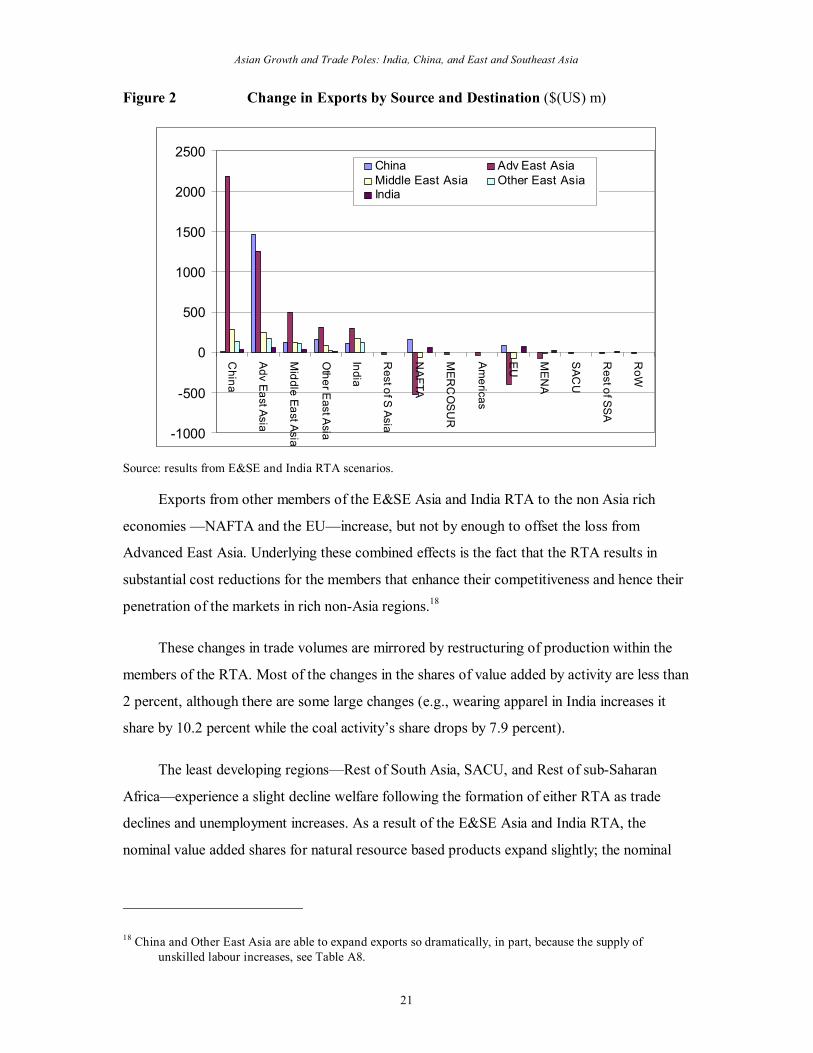
21

Figure 2 Change in Exports by Source and Destination ($(US) m)

1000

500

0

500

1000

1500

2000

2500

China

Adv East Asia

Middle East Asia

Other E

ast Asia

India

Rest of S Asia

NAFTA

MER

COSUR

Americas

EU

MEN

A

SAC

U

Rest of SSA

RoW

China Adv East Asia Middle East Asia Other East Asia India

Source: results from E&SE and India RTA scenarios.

Exports from other members of the E&SE Asia and India RTA to the non Asia rich

economies —NAFTA and the EU—increase, but not by enough to offset the loss from

Advanced East Asia. Underlying these combined effects is the fact that the RTA results in

substantial cost reductions for the members that enhance their competitiveness and hence their

penetration of the markets in rich nonAsia regions. 18

These changes in trade volumes are mirrored by restructuring of production within the

members of the RTA. Most of the changes in the shares of value added by activity are less than

2 percent, although there are some large changes (e.g., wearing apparel in India increases it

share by 10.2 percent while the coal activity’s share drops by 7.9 percent).

The least developing regions—Rest of South Asia, SACU, and Rest of subSaharan

Africa—experience a slight decline welfare following the formation of either RTA as trade

declines and unemployment increases. As a result of the E&SE Asia and India RTA, the

nominal value added shares for natural resource based products expand slightly; the nominal

18 China and Other East Asia are able to expand exports so dramatically, in part, because the supply of unskilled labour increases, see Table A8.


22

value added shares of textiles and apparel decline; and the nominal value added shares of most

other manufactured goods expand slightly (the change is less than one percent, see figure A2).

4. Efficiency Gains in Developing Asia

The summary macroeconomic measures demonstrate that the gains from productivity growth

within India and China in isolation are largely concentrated within that region (see Table 5);

and while the spillover effects on other regions are limited they are positive. Most of this gain

is generated by the expansion of exports by the growing region, since a region becomes more

competitive with productivity growth, and this produces some small declines in export volumes

by other regions: only one region, NAFTA, experiences a marginal increase. These summary

measures are supported by the detailed estimates of the changes in bilateral trade flows.

Table 5 Summary Macroeconomic and Welfare Results for Growth Scenarios

Absorption ($US bn) Absorption (%) Welfare

($US bn) Export supply (%)

Base India 10% growth

China 10% growth

Developing Asia 10% growth


India 10% growth

China 10% growth


China 1,224 0.00 8.98 9.06 110.83 0.01 10.60 10.54 Adv East Asia 5,266 0.00 0.12 0.21 10.93 0.01 0.08 0.14 Middle East Asia 182 0.10 0.37 6.93 12.61 0.01 0.04 8.61

Other East Asia 317 0.05 0.21 7.75 24.56 0.07 0.20 9.86

India 476 7.95 0.00 7.91 37.69 11.25 0.14 11.00 Rest of S Asia 150 0.07 0.01 0.09 0.13 0.04 0.16 0.34 NAFTA 11,764 0.01 0.06 0.09 10.64 0.01 0.02 0.01 MERCOSUR 917 0.01 0.05 0.09 0.79 0.01 0.04 0.08 Americas 485 0.05 0.07 0.16 0.76 0.04 0.09 0.19 EU 8,668 0.01 0.05 0.09 7.95 0.00 0.02 0.04 MENA 1,017 0.08 0.20 0.45 4.60 0.05 0.17 0.35 SACU 113 0.07 0.15 0.26 0.29 0.01 0.06 0.09 Rest of SSA 207 0.15 0.33 0.68 1.41 0.00 0.06 0.06 RoW 492 0.04 0.17 0.28 1.36 0.03 0.09 0.17

Source: results from China growth, India growth, and Developing Asia growth scenarios.

There are few surprises in the results considered so far. In general, the prospective

members of an RTA gain while non members lose small amounts, and the impacts of growth

—efficiency gains— far outweigh the potential static benefits of integration. The impacts on

other regions are mixed: generally positive in welfare and import terms but somewhat negative

in terms of exports, as the regions that are not experiencing efficiency gains lose


23

competitiveness. The termsoftrade results are also consistent with these patterns in the results

(Table 6) in that the terms of trade deteriorate for those regions experiencing efficiency gains,

but appreciate slightly for those regions not experiencing the efficiency gains. Consequently,

the percentage increases in absorption for growing fall short of the efficiency gains.

The terms of trade for sub groups of commodities, i.e., agricultural, natural resource,

food, manufacturing, utility and service commodities, follow much the same pattern, with the

deterioration in the terms of trade more marked for the broad commodity groups where the

efficiency gains are realised (food, manufacturing, utility, and service commodities). It is

notable that the termsoftrade effects are most pronounced in those groups of commodities

that are least traded.

Table 6 Terms of Trade – Productivity Growth in Developing Asia

Overall Agriculture Natural Resources Food Industry Utility Service

China 95.7 98.5 96.0 97.9 96.2 98.1 94.3 Adv East Asia 101.1 101.3 100.9 100.8 101.5 100.4 101.2 Middle East Asia 96.3 99.6 99.1 98.7 96.7 96.5 93.7 Other East Asia 96.3 99.2 98.0 98.5 95.6 94.2 92.9 India 94.7 98.7 92.6 98.8 95.7 92.7 93.0 Rest of S Asia 100.5 100.1 101.8 100.6 100.6 100.4 100.9 NAFTA 100.6 100.4 100.0 100.3 100.5 100.1 101.1 MERCOSUR 100.5 100.4 100.4 100.1 100.2 100.1 100.8 Americas 100.6 100.0 100.9 100.1 100.2 100.1 100.8 EU 100.3 99.9 100.0 100.1 100.2 100.0 100.9 MENA 101.3 100.1 100.9 100.3 100.9 100.0 100.7 SACU 100.5 99.9 100.3 100.3 100.4 99.8 100.7 Rest of SSA 101.3 100.3 100.8 100.2 100.8 100.1 100.6 RoW 100.6 100.3 100.2 100.2 100.5 100.1 100.9

Source: results from Developing Asia growth scenario.

Efficiency gains in developing Asia affect the least developed regions. The small

magnitudes of the macroeconomic implications of efficiency gains in developing Asia for other

regions suggest that the impacts upon their economies are likely to be small. For the least

developed regions —Rest of South Asia, Rest of sub Saharan Africa and SACU— the welfare

gains is only $(US) 1.8bn, which while positive is less than an 0.4 percent increase, although in

proportionate terms it is some 3.5 times the proportionate gains experienced by other non

growing regions. Much of the benefit that accrues to regions that are not experiencing

efficiency gains comes through declining import prices.


24

Figure 3 Aggregate Exports by Least Developed Regions (% change)

4.0

2.0

0.0

2.0

4.0

6.0

8.0

10.0

12.0

Crops

Livestock Coal

Oil and gas

Other m

inerals Meat products

Other foods

Textiles Wearing apparel

Wood and paper

Petroleum

and coal Chem

ical etc Basic m

etal etc Motor vehicles

Transport equipment

Electronic equipm

ent Machinery and equipm

ent Other m

anufacturing Utilities

Construction

Trade and transport Business services

Other services

Rest of S Asia SACU Rest of SSA


Trade patterns change in least developed regions as a result of growth in developing

Asia. Figures 3 and 4 illustrate the proportion changes in trade volumes by commodity for the

least developed regions. While overall export volumes decline by small amounts (Table 5), the

declines in export volumes are concentrated in manufactured commodities, while there are

appreciable increases in primary commodity exports (the change for oil and gas from the Rest

of South Asia is misleading since it is from a small base). There is evidence from the export

data that the experiences of least developed countries in Asia will differ from those in Africa.

The Asian regions see increases in exports across most commodities, with declining exports

concentrated in textiles and wearing apparel that accounted for nearly 60 percent of exports in

the base period. Consequently there is evidence to suggest that the least developed countries

will become less able to compete in those sectors that they are currently seeking to expand,

and will be encouraged to expand production in primary commodity sectors.


25

Figure 4 Aggregate Imports by Least Developed Regions (% change)

4.0

3.0 2.0

1.0 0.0

1.0 2.0

3.0 4.0

5.0

Crops

Livestock

Coal

Oil and gas

Other m

inerals

Meat products

Other foods

Textiles

Wearing apparel

Wood and paper

Petroleum

and coal

Chem

ical etc

Basic m


Transport equipment

Electronic equipm


ent

Other m

anufacturing

Utilities

Construction

Trade and transport

Business services

Other services



This is further emphasised by the imports results (Figure 4), which indicate increasing

imports across nearly all nonprimary commodities for all least developed regions, together

with declining imports of primary commodities. These results are consistent with greater

penetration of the secondary and tertiary markets in least developed regions, which induce

shifts towards the primary commodity sectors; shifts that are further encouraged by growing

demand for primary commodity inputs in the growing regions.

The results for the direction of trade flows, Figures 5 and 6, demonstrate that the least

developed countries will increasingly source imports from, and direct exports to, the

developing Asian economies. To a large extent this is achieved by redirecting exports from the

traditional markets of the EU and NAFTA, while shifting resources towards the primary

commodity sectors (see below). 19 An examination of the bilateral trade results shows that the

dominant factors are the declining prices of exports of commodities from the developing Asian

19 The Rest of South Asia and SACU also reduce imports from the EU and NAFTA.


26

economies coupled with an escalating demand by those economies for inputs of primary

commodities. Indeed total supply of coal, oil and gas and other minerals to the developing

Asian economies increases by nearly 10 percent. Notably, agricultural commodity supplies

increase by less than half the rates for fuel and mineral commodities.

Figure 5 Changes in Exports by Destination from Least Developed Regions

($US millions)

300

100

100

300

500

700

China

Adv E

ast Asia

Middle E

ast Asia

Other E

ast Asia

India

Rest of S Asia

NAFTA

MERCOSUR

Americas

EU

MENA

SACU

Rest of S

SA

RoW

Destination Region




27

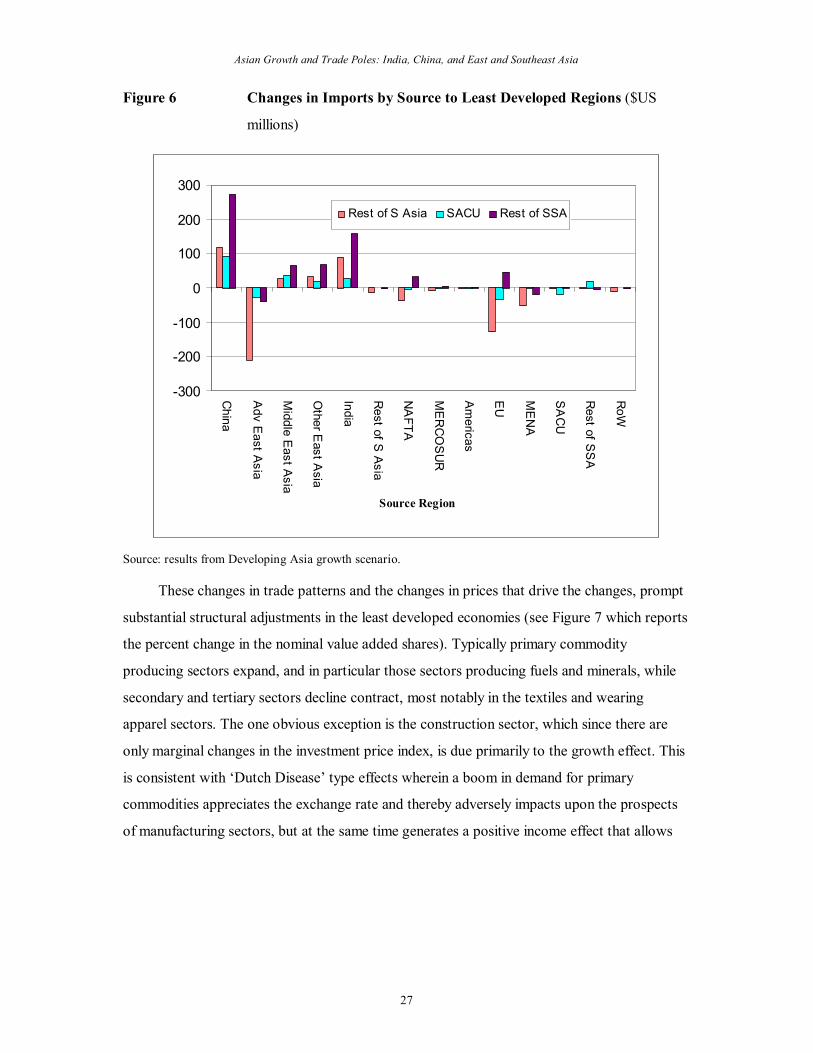
Figure 6 Changes in Imports by Source to Least Developed Regions ($US

millions)

300

200

100

0

100

200

300

China

Adv E

ast Asia

Middle E

ast Asia

Other E

ast Asia

India

Rest of S

Asia

NAFTA

MERCOSUR

Americas

EU

MENA

SACU

Rest of S

SA

RoW

Source Region



These changes in trade patterns and the changes in prices that drive the changes, prompt

substantial structural adjustments in the least developed economies (see Figure 7 which reports

the percent change in the nominal value added shares). Typically primary commodity

producing sectors expand, and in particular those sectors producing fuels and minerals, while

secondary and tertiary sectors decline contract, most notably in the textiles and wearing

apparel sectors. The one obvious exception is the construction sector, which since there are

only marginal changes in the investment price index, is due primarily to the growth effect. This

is consistent with ‘Dutch Disease’ type effects wherein a boom in demand for primary

commodities appreciates the exchange rate and thereby adversely impacts upon the prospects

of manufacturing sectors, but at the same time generates a positive income effect that allows


28

for increases in absorption, which, given the behavioural assumptions underlying this model,

produces increases in investment. 20

Figure 7 Shares of Value Added by Activity in Least Developed Region (%

change)

4.00

3.00

2.00

1.00

0.00

1.00

2.00

3.00

4.00

5.00

Crops

Livestock Coal

Oil and gas

Other m


Other foods

Textiles Wearing apparel

Wood and paper

Petroleum

and coal Chem

ical etc Basic m


Transport equipment

Electronic equipm


ent Other m

anufacturing Utilities

Construction

Trade and transport Business services

Other services



It is notable that in this case the exchange rates appreciate for the African regions but

depreciate for the Rest of South Asia, which is consistent with the relative importance of

primary commodity exports in those regions. Overall there is an expansion of trade between

the least developed regions and the developing Asia regions, but the increases in absolute trade

export values are appreciably greater for the African regions than the Rest of South Asia,

which is a reflection of the greater presence of the African regions as sources of natural

resource based primary commodities.

20 This evidence supports the concerns raised by Goldstein et al., (2006) about the potential for ‘Dutch Disease’ effects in Africa.


29

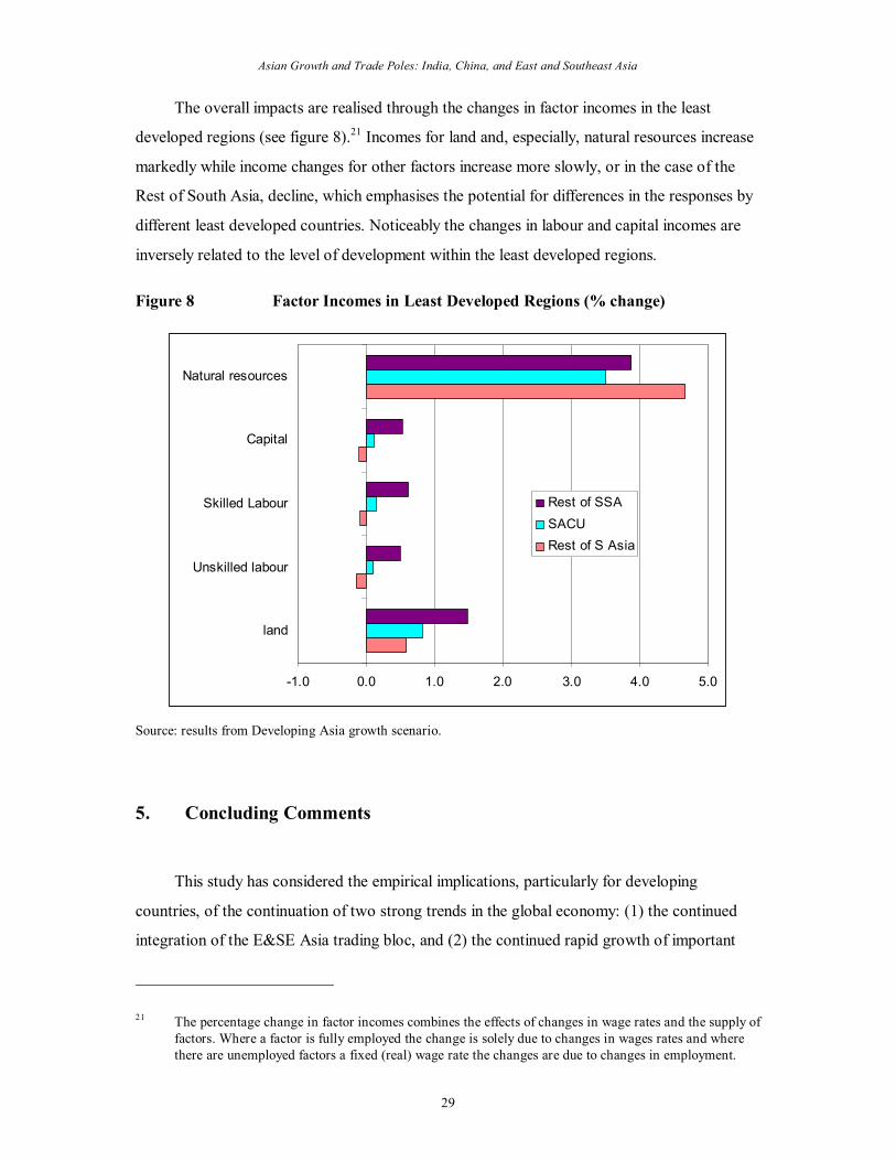
The overall impacts are realised through the changes in factor incomes in the least

developed regions (see figure 8). 21 Incomes for land and, especially, natural resources increase

markedly while income changes for other factors increase more slowly, or in the case of the

Rest of South Asia, decline, which emphasises the potential for differences in the responses by

different least developed countries. Noticeably the changes in labour and capital incomes are

inversely related to the level of development within the least developed regions.

Figure 8 Factor Incomes in Least Developed Regions (% change)

1.0 0.0 1.0 2.0 3.0 4.0 5.0

land

Unskilled labour

Skilled Labour

Capital

Natural resources

Rest of SSA SACU Rest of S Asia


5. Concluding Comments

This study has considered the empirical implications, particularly for developing

countries, of the continuation of two strong trends in the global economy: (1) the continued

integration of the E&SE Asia trading bloc, and (2) the continued rapid growth of important

21 The percentage change in factor incomes combines the effects of changes in wage rates and the supply of factors. Where a factor is fully employed the change is solely due to changes in wages rates and where there are unemployed factors a fixed (real) wage rate the changes are due to changes in employment.


30

countries in Asia, with increasing pressure on world markets for manufactures and primary

commodities. The results indicate that:

• The continued integration of E&SE Asia, with the effective creation of a free

trade area, would increase welfare in the region and generate small losses for

countries outside the bloc.

• The inclusion of India in the trade bloc would lead to a welfare gain for India,

and also additional substantial gains for existing bloc members. The impacts on

countries outside the bloc are small.

• Continued integration involves significant changes in the structure of production

in, and trade by, the E&SE Asia bloc. Advanced Asian countries redirect exports

from the EU and the US toward countries within the bloc, while other members

increase their exports to the EU and US.

• Increased growth in the developing countries in Asia leads to significant terms

oftrade and welfare gains for the other developing countries, as their import

prices fall and world prices of primary exports rises.

• Improvements in the terms of trade lead to Dutch Disease problems for

developing countries which export primary commodities. These countries will be

less able to compete in world markets for manufactures, where they have been

seeking to expand exports, and gain instead from expanding primary exports.

While there are increases in welfare, the changes in the structure of trade and

production away from manufactures may hinder development in the longer term,

particularly in Africa.

The GLOBE model used in this study is neoclassical in spirit and provides a simulation

laboratory for analysing the impact of global shocks such as changes in trade policy and

differential growth in a consistent, multiregion, general equilibrium framework. While the

results indicate significant impacts from differential growth and tariff policy, the model is

narrowly focused on standard competitive market mechanisms, omitting many complications.

For example, the study assumes that further integration in E&SE Asia involves only the

elimination of trade barriers (i.e., ‘shallow integration’), and makes no allowance for deeper

transformations in the patterns of production and trade linked to behindtheborder institutional

changes (i.e., ‘deep integration’), which are likely to be an important part of the process of


31

further integration in the region. 22 The inclusion of issues of institutional change, externalities,

and deep integration into empirical trade models is a new and difficult area of active research,

with much to be done, but also much to be gained in terms of deeper understanding of the links

between expanded trade and economic performance.

With respect to the least developed regions, the study concentrates on broad regional

aggregates, which obscures the variety of experience likely to confront the least developed

regions. In particular the Dutch Disease effects identified in the analyses indicate that those

regions that are rich in natural resources are likely to gain appreciably from increases in world

prices of primary commodities, and that these gains will counteract the loses associated with

reducing competitiveness in other commodity markets. However, within these regional

aggregates, countries that are not natural resource rich are likely to suffer losses far greater

than implied by this study. Aggregation is always a difficult issue in empirical models, with

tradeoffs between expanding the domain of applicability of the model, straining data sources,

and adding complexity that makes analysis of the major forces at work more difficult.

The changes in the global patterns of production and trade associated with the very high

growth rates in the Asian Drivers are producing a period of major structural readjustment in

the global economy. While the emerging Asian economies remain a relatively small part of the

global economy, they are growing rapidly and expanding their role in global markets. Although

trade expansion is typically a positivesum game, the benefits of the gains are not distributed

equally, and there is no a priori reason that all regions will gain. The results from this study

indicate that some economies will in fact lose, and since many of the economies likely to lose

are the least developed regions of the world, it is argued that it is important to develop the

analytical capacity to understand the forces unleashed by the current period of rapid structural

adjustment.

References

Antkiewicz, A. and Whalley, J., (2005). ‘China’s New Regional Trade Agreements’, The World Economy, 28 (10), 15391557

22 Consider, for example, the sorts of institutional and structural changes that have been part of the process of deep integration in the EU.


32

Baysan, T., Panagariya, A. and Pitigala, N., (2006). ‘The Preferential Trading in South Asia,’ World Bank Working Paper 3813. Washington: World Bank.

Dervis, K., de Melo, J. and Robinson, S., (1982). General Equilibrium Models for Development Policy. Washington: World Bank.

Devarajan, S., Lewis, J.D. and Robinson, S., (1990). ‘Policy Lessons from TradeFocused, TwoSector Models’, Journal of Policy Modeling, 12, 625657.

Dimaranan, B. V., (ed) (2006). Global Trade, Assistance, and Production: The GTAP 6 Data Base. Center for Global Trade Analysis, Purdue University.

Evans, D., Kaplinsky, R. and Robinson, S., (2006) ‘Deep and Shallow Integration in Asia: Towards a Holistic Account.’ IDS Bulletin,. 37(1). Institute of Development Studies.

Goldstein, A., Pinaud, N., Reisen, H. and Chen, X., (2006). The Rise of China and India: What’s in It for Africa? Paris: OECD Development Centre.

Greenaway, D. and Milner, C., (1991). ‘Fiscal Dependence on Trade Taxes and Trade Policy Reform’, Journal of Development Studies, 27, 94132.

Hertel, T.W., (1997). Global Trade Analysis: Modeling and Applications. Cambridge: Cambridge University Press.

Kaplinsky, R., (2005), Globalization, Poverty and Inequality: Between a Rock and a Hard Place. Cambridge: Polity.

Lee, JW. and Park, I., (2005). ‘Free Trade Areas in East Asia: Discriminatory or Non discriminatory?’ The World Economy, 28 (1), 2148.

Lee, JW. and Shin, K., (2006). ‘Does Regionalism Lead to More Global Trade Integration in East Asia?’ North American Journal of Economics and Finance, 17, 283301.

Lewis, J. D., Robinson, S. and Wang, Z., (1995). ‘Beyond the Uruguay Round: The Implications of an Asian Free Trade Area’, China Economic Review, 6, 3792.

de Melo, J and Robinson, S., (1989). ‘Product Differentiation and the Treatment of Foreign Trade in Computable General Equilibrium Models of Small Economies’, Journal of International Economics, 27, 4767.

McDonald, Scott (2006). Deriving Reduced Form Global Social Accounting Matrices from GTAP Data, mimeo.

McDonald, S, and Thierfelder, K., (2004). ‘Deriving a Global Social Accounting Matrix from GTAP version 5 Data’, GTAP Technical Paper 23. Global Trade Analysis Project: Purdue University.

McDonald, S., Robinson, S. and Thierfelder, K., (2005). ‘A SAM Based Global CGE Model using GTAP Data’, Sheffield Economics Research Paper 2005:001. The University of Sheffield.

McDonald, S., Robinson, S. and Thierfelder, K., (2006a). ‘Impact of Switching Production to Bioenergy Crops: The Switchgrass Example,’ Energy Economics, 28, 243265.

Pyatt, G., 1987, ‘A SAM Approach to Modeling’, Journal of Policy Modeling, 10, 327352.


33

Robinson, S., Kilkenny, M. and Hanson, K., 1990, ‘USDA/ERS Computable General Equilibrium Model of the United States’, Economic Research Service, USDA, Staff Report AGES 9049.

Schiff, M., and Winters, A. L., (2003). Regional Integration and Development. Washington, DC: The World Bank.

Taylor, Lance and Rudiger von Arnim (2007). Modelling the Impact of Trade Liberalisation: A Critique of Computable General Equilibrium Models. Oxfam International Research Report.

van der Mensbrugghe, D., (2006). Linkage Technical Reference Document: Version 6.0. Washington, DC: World Bank.

World Bank, (2005). Global Economic Prospects, 2005: Trade, Regionalism, and Development. Washington, DC: The World Bank.

Appendix

Table A1 Commodity and Activity Account Mappings

GTAP Accounts Model Accounts GTAP Accounts Model Accounts Paddy rice Crop agriculture Wood products Wood and paper products Wheat Crop agriculture Paper products publishing Wood and paper products Cereal grains nec Crop agriculture Petroleum coal products Petroleum and coal products

Vegetables fruit nuts Crop agriculture Chemical rubber plastic prods Chemical rubber & plastic products

Oil seeds Crop agriculture Mineral products nec Basic metal & mineral products

Sugar cane sugar beet Crop agriculture Ferrous metals Basic metal and mineral products

Plantbased fibers Crop agriculture Metals nec Basic metal and mineral products

Crops nec Crop agriculture Metal products Other manufacturing Cattle sheep goats horses Animal agriculture Motor vehicles and parts Motor vehicles and parts Animal products nec Animal agriculture Transport equipment nec Other transport equipment Raw milk Animal agriculture Electronic equipment Electronic equipment Wool silkworm cocoons Animal agriculture Machinery and equipment nec Machinery and equipment Forestry Crop agriculture Manufactures nec Other manufacturing Fishing Animal agriculture Electricity Utilities Coal Coal Gas manufacture distribution Utilities Oil Oil and gas Water Utilities Gas Oil and gas Construction Construction Minerals nec Other minerals Trade Trade and transport Meat: cattle sheep goats horse Meat products Transport nec Trade and transport Meat products nec Meat products Sea transport Trade and transport Vegetable oils and fats Other foods Air transport Trade and transport Dairy products Meat products Communication Trade and transport Processed rice Other foods Financial services nec Business services Sugar Other foods Insurance Business services


34

Food products nec Other foods Business services nec Business services Beverages and tobacco products Other foods Recreation & other services Other services

Textiles Textiles PubAdmin Defence Health Educat Other services

Wearing apparel Wearing apparel Dwellings Other services Leather products Wearing apparel

Table A2 Factor Account Mappings

GTAP Accounts Model Accounts Land Land Unskilled labour Unskilled labour Skilled labour Skilled Labour Capital Capital Natural Resources Natural resources

Table A3 Region Account Mappings

GTAP Accounts Model Accounts GTAP Accounts Model Accounts Australia Advanced East Asia Canada NAFTA New Zealand Advanced East Asia United States NAFTA Japan Advanced East Asia Mexico NAFTA Korea Advanced East Asia Argentina MERCOSUR plus Taiwan Advanced East Asia Brazil MERCOSUR plus Singapore Advanced East Asia Chile MERCOSUR plus China China Colombia MERCOSUR plus Hong Kong China Uruguay Rest of the Americas Rest of East Asia Middle East Asia Rest of South America Rest of the Americas Malaysia Middle East Asia Central America Rest of the Americas Rest of Oceania Middle East Asia Rest of FTAA Rest of the Americas Thailand Middle East Asia Rest of the Caribbean Rest of the Americas Indonesia Other East Asia Rest of North America Rest of the Americas Philippines Other East Asia Peru Rest of the Americas Vietnam Other East Asia Venezuela Rest of the Americas Rest of Southeast Asia Other East Asia Rest of Andean Pact Rest of the Americas India India Rest of Europe Rest of the World Bangladesh Rest of South Asia Albania Rest of the World Sri Lanka Rest of South Asia Bulgaria Rest of the World Rest of South Asia Rest of South Asia Croatia Rest of the World Austria European Union Romania Rest of the World Belgium European Union Russian Federation Rest of the World Denmark European Union Rest of Former Soviet Union Rest of the World Finland European Union Turkey Middle East and North Africa France European Union Rest of Middle East Middle East and North Africa Germany European Union Morocco Middle East and North Africa United Kingdom European Union Tunisia Middle East and North Africa Greece European Union Rest of North Africa Middle East and North Africa

Ireland European Union Botswana Southern Africa Customs Union

Italy European Union South Africa Southern Africa Customs Union

Luxembourg European Union Rest of South African CU Southern Africa Customs Union

Netherlands European Union Malawi Rest of subSaharan Africa Portugal European Union Mozambique Rest of subSaharan Africa


35

Spain European Union Tanzania Rest of subSaharan Africa Sweden European Union Zambia Rest of subSaharan Africa Switzerland European Union Zimbabwe Rest of subSaharan Africa Rest of EFTA European Union Rest of SADC Rest of subSaharan Africa Cyprus European Union Madagascar Rest of subSaharan Africa Czech Republic European Union Uganda Rest of subSaharan Africa Hungary European Union Rest of SubSaharan Africa Rest of subSaharan Africa Malta European Union Poland European Union Slovakia European Union Slovenia European Union Estonia European Union Latvia European Union Lithuania European Union

Table A.4 Export Shares by Least Developed Countries

From Rest of South Asia to : From SACU to: From Rest of SSA to:

China E&SE Asia India China

E&SE Asia India China

E&SE Asia India

Crops 0.02 0.11 0.07 0.03 0.13 0.00 0.06 0.10 0.04 Livestock 0.03 0.39 0.06 0.06 0.06 0.00 0.12 0.06 0.04 Coal 0.05 0.09 0.11 0.00 0.06 0.03 0.03 0.08 0.01 Oil and gas 0.01 0.60 0.15 0.00 0.01 0.01 0.06 0.08 0.00 Other minerals 0.29 0.25 0.07 0.20 0.22 0.02 0.11 0.11 0.04 Meat products 0.01 0.01 0.75 0.01 0.04 0.00 0.01 0.04 0.00 Other foods 0.02 0.13 0.02 0.02 0.13 0.00 0.02 0.07 0.00 Textiles 0.07 0.09 0.01 0.01 0.07 0.01 0.01 0.03 0.01 Wearing apparel 0.01 0.03 0.00 0.02 0.06 0.00 0.01 0.02 0.01 Wood and paper 0.00 0.07 0.11 0.02 0.19 0.01 0.01 0.01 0.01 Petroleum and coal 0.01 0.20 0.01 0.01 0.06 0.01 0.01 0.09 0.01 Chemical etc 0.06 0.10 0.17 0.03 0.09 0.04 0.00 0.04 0.10 Basic metal etc 0.01 0.10 0.26 0.03 0.23 0.10 0.02 0.08 0.01 Motor vehicles 0.01 0.14 0.00 0.02 0.24 0.00 0.01 0.02 0.00 Transport equipment 0.06 0.02 0.01 0.02 0.02 0.00 0.00 0.14 0.04 Electronic equipment 0.08 0.45 0.01 0.02 0.06 0.01 0.02 0.07 0.00 Machinery and equipment 0.02 0.29 0.02 0.03 0.04 0.01 0.04 0.05 0.01 Other manufacturing 0.00 0.10 0.01 0.03 0.01 0.00 0.00 0.02 0.02 Utilities 0.03 0.03 0.05 0.01 0.02 0.01 0.00 0.01 0.00 Construction 0.07 0.23 0.00 0.04 0.27 0.00 0.06 0.21 0.01 Business services 0.04 0.18 0.01 0.05 0.16 0.01 0.03 0.18 0.01 Other services 0.03 0.07 0.00 0.03 0.12 0.00 0.03 0.09 0.01


Table A5 Import Shares by Least Developed Countries

Rest of South Asia's imports from :

SACU's imports from: Rest of SSA's imports from:

China E&SE Asia India China

E&SE Asia India China

E&SE Asia India

Crops 0.04 0.22 0.15 0.03 0.11 0.03 0.03 0.09 0.02 Livestock 0.11 0.32 0.12 0.05 0.11 0.00 0.04 0.08 0.01 Coal 0.02 0.48 0.37 0.00 0.92 0.00 0.05 0.13 0.03


36

Oil and gas 0.00 0.03 0.00 0.00 0.04 0.00 0.01 0.02 0.00 Other minerals 0.05 0.33 0.25 0.02 0.07 0.02 0.01 0.02 0.04 Meat products 0.00 0.68 0.04 0.02 0.23 0.00 0.00 0.15 0.02 Other foods 0.00 0.38 0.15 0.01 0.15 0.05 0.04 0.19 0.03 Textiles 0.25 0.50 0.10 0.15 0.33 0.04 0.28 0.21 0.16 Wearing apparel 0.17 0.33 0.08 0.36 0.08 0.08 0.31 0.26 0.05 Wood and paper 0.05 0.43 0.10 0.02 0.08 0.00 0.02 0.09 0.03 Petroleum and coal 0.01 0.19 0.02 0.01 0.01 0.01 0.04 0.02 0.01 Chemical etc 0.10 0.36 0.09 0.03 0.12 0.01 0.05 0.12 0.06 Basic metal etc 0.05 0.41 0.12 0.04 0.22 0.01 0.03 0.11 0.06 Motor vehicles 0.07 0.57 0.10 0.00 0.22 0.00 0.02 0.19 0.02 Transport equipment 0.10 0.34 0.11 0.01 0.04 0.00 0.04 0.38 0.02 Electronic equipment 0.14 0.49 0.02 0.08 0.21 0.00 0.05 0.15 0.01 Machinery and equipment 0.12 0.32 0.07 0.03 0.17 0.01 0.07 0.11 0.02 Other manufacturing 0.14 0.31 0.07 0.09 0.13 0.03 0.13 0.07 0.06 Utilities 0.02 0.04 0.01 0.00 0.00 0.00 0.01 0.01 0.00 Construction 0.04 0.20 0.01 0.03 0.19 0.00 0.04 0.20 0.00 Business services 0.04 0.15 0.01 0.03 0.12 0.01 0.04 0.14 0.02 Other services 0.02 0.10 0.01 0.02 0.09 0.00 0.02 0.08 0.01


Table A6 Average Tariff Rates – E&SE Asia and India

China Adv East Asia

Middle East Asia

Other East Asia

India

Crops 0.43 0.47 0.16 0.04 0.23 Livestock 0.04 0.04 0.05 0.03 0.14 Coal 0.01 0.00 0.01 0.05 0.43 Oil and gas 0.00 0.02 0.00 0.02 0.15 Other minerals 0.01 0.00 0.01 0.02 0.11 Meat products 0.08 0.40 0.06 0.09 0.57 Other foods 0.10 0.20 0.27 0.21 0.79 Textiles 0.15 0.07 0.12 0.13 0.26 Wearing apparel 0.04 0.11 0.11 0.14 0.28 Wood and paper 0.07 0.02 0.10 0.06 0.22 Petroleum and coal 0.06 0.02 0.01 0.06 0.17 Chemical etc 0.11 0.03 0.08 0.05 0.31 Basic metal etc 0.06 0.02 0.08 0.05 0.33 Motor vehicles 0.29 0.09 0.36 0.21 0.40 Transport equipment 0.04 0.00 0.06 0.16 0.19 Electronic equipment 0.07 0.00 0.02 0.01 0.15 Machinery and equipment 0.11 0.02 0.06 0.04 0.25

Other manufacturing 0.07 0.02 0.10 0.09 0.34



37

Table A7 Sectoral Export Shares of Production for Selected Regions

Percent of production that is exported

China Adv East Asia

Middle East Asia

Other East Asia India SACU Rest of

SSA Crops 2.6 8.0 21.9 11.9 2.9 29.3 18.2 Livestock 1.8 6.9 6.4 2.7 0.4 7.0 2.3 Coal 23.6 66.4 2.1 66.1 1.3 30.8 1.4 Oil and gas 3.7 33.9 41.3 55.8 0.0 38.8 87.4 Other minerals 1.8 20.7 28.2 35.5 39.6 44.0 24.0 Meat products 7.3 13.8 31.7 4.3 6.8 7.4 3.1 Other foods 5.0 3.7 41.0 12.7 7.5 18.1 8.6 Textiles 16.1 42.3 33.1 29.5 20.7 18.4 19.6 Wearing apparel 55.1 12.8 52.1 69.9 68.1 45.9 28.9 Wood and paper 16.6 5.3 46.8 48.2 5.4 24.0 15.3 Petroleum and coal 5.1 8.8 14.5 8.2 6.0 17.4 11.5 Chemical etc 11.3 19.9 47.4 25.1 12.6 24.9 13.5 Basic metal etc 5.7 14.9 31.2 26.0 8.4 63.3 39.7 Motor vehicles 5.4 27.5 17.9 5.8 5.9 32.5 55.0 Transport equipment 16.6 46.0 47.8 34.2 6.0 35.8 65.8 Electronic equipment 54.9 43.8 91.4 79.9 13.0 48.8 38.0 Machinery and equipment 21.5 40.4 60.4 58.3 11.3 39.8 42.1 Other manufacturing 32.1 13.5 35.2 27.2 25.3 55.4 18.9 Utilities 0.7 0.1 1.3 0.2 0.0 2.4 8.5 Construction 0.3 0.6 2.4 0.7 0.0 0.1 0.6 Trade and transport 0.0 0.0 0.0 0.0 0.0 0.0 0.0 Business services 13.0 3.4 32.0 7.4 14.9 4.0 9.4 Other services 1.5 0.7 5.4 2.1 1.0 1.5 3.9


Table A8 Unskilled Labour Supply (% change)

E&SE Asia RTA

E&SE Asia & India RTA

India 10% growth

China 10% growth

Developing E&SE Asia 10% growth

China 2.4 2.4 0.0 5.1 5.1 Other East Asia 1.7 1.9 0.0 0.0 5.6 India 0.2 1.3 4.3 0.1 4.1 Rest of S Asia 0.3 0.4 0.0 0.1 0.2 SACU 0.1 0.2 0.0 0.1 0.1 Rest of SSA 0.1 0.1 0.1 0.2 0.5

Source: model simulation results for each scenario.


38

Figure A1 Global GDP (expenditure measure)

Adv East Asia 17%

Americas 1%

MERCOSUR 3%

EU 28%

MENA 3%

SACU 0%

Rest of SSA 1%

RoW 2% China

4%

Other East Asia 1%

Middle East Asia 1%

India 1%

Rest of S Asia 0%

NAFTA 38%


Figure A2 Shares of Value Added by Activity in Least Developed Region (%

change)

4

3

2

1

0

1

2

3

Crops

Livestock Coal

Oil and gas

Other m


Other foods

Textiles Wearing

Wood and

Petroleum

and Chem

ical etc Basic m

etal Motor vehicles

Transport Electronic

Machinery and

Other

Utilities

Construction

Trade and Business

Other services


Source: results from E&SE Asia and India RTA.

Asian Growth and Trade Poles: India, China, and East and ... · Asian Growth and Trade Poles:...

Documents

Transcript of Asian Growth and Trade Poles: India, China, and East and ... · Asian Growth and Trade Poles:...