Asian Development Policy Revie2)-111-132.pdfThis study conducts a joint evaluation of nonlinear...

Asian Development Policy Review, 2019, 7(2): 111-132

111

© 2019 AESS Publications. All Rights Reserved.

REGIME-DEPENDENT EFFECTS ON STOCK MARKET RETURN DYNAMICS: EVIDENCE FROM SAARC COUNTRIES

Zobia Israr Ahmed1+ Khalid Mustafa2

1BAMM PECHS Government College for Women, Karachi, Pakistan

2Department of Economics, University of Karachi, Pakistan

(+ Corresponding author)

ABSTRACT Article History Received: 24 December 2018 Revised: 30 January 2019 Accepted: 6 March 2019 Published: 10 May 2019

Keywords Markov switching model Stock market returns Exchange rate market Macroeconomic factors Financial crises

JEL Classification: C22; G17; F31.

This study empirically examines the link between stock market returns and exchange rate fluctuations using monthly data ranging from 1993 to 2016 for selected SAARC countries (Bangladesh, India, Pakistan, and Sri Lanka). In the presence of other macroeconomic factors, dynamic links in the financial markets are investigated using Hamilton's Markov switching approach. The multivariate analysis reveals that stock market returns develop in accordance with two different regimes: during a crisis and when there is no crisis. The study discovered evidence of switching suggesting that stock markets have persistent volatility in bullish trends and are influenced more by currency returns during both calm and turbulent periods. However, stock markets with persistent volatility in bearish trends are influenced more by other macroeconomic factors, in both periods. This implies that movements in the stock market are regime-dependent and transition probabilities between regimes can be affected by certain macroeconomic factors.

Contribution/Originality: This study contributes to the existing literature by examining whether there is a

switching behavior in South Asian stock markets and whether regime-switching behavior is influenced by a number

of factors that directly or indirectly affect internal and external economic, financial, and political elements during

times of crisis and stability.

1. INTRODUCTION

Dramatic changes in the behavior of many financial time series mainly correlate with such incidents as financial

shocks, crises, wars, or variations in governmental monetary policy. Stock market performance is directly or

indirectly affected by local and international crises, due to the impact on currency markets and other

macroeconomic factors. Similarly, unforeseen variations in inflation forecasts, contractionary monetary policies, and

an increase in oil prices, exert a downward stress on financial market valuations, leading to uncertainty in

economies’ cash flows and further reactions in the financial markets. Therefore, imbalances in the economy result in

volatile exchange rates and capital markets.

This study aims to empirically demonstrate the dynamic relationship between changes in currency exchange

rates and stock market returns in selected SAARC countries.1 This interrelationship is important for economic

1 Only the emerging SAARC (South Asian Association for Regional Cooperation) countries were selected: Bangladesh, India, Pakistan, and Sri

Lanka.

Asian Development Policy Review ISSN(e): 2313-8343 ISSN(p): 2518-2544 DOI: 10.18488/journal.107.2019.72.111.132 Vol. 7, No. 2, 111-132 © 2019 AESS Publications. All Rights Reserved. URL: www.aessweb.com

http://crossmark.crossref.org/dialog/?doi=10.18488/journal.107.2019.72.111.132&domain=pdf&date_stamp=2017-01-14

https://orcid.org/0000-0002-1961-952X

http://www.aessweb.com/

http://www.aessweb.com/journals/June2019/5008/4561


112


policies and decisions on international capital budgeting, particularly when negative shocks affecting one market

are rapidly transmitted to the other markets. Following the Financial Crisis of 2008, the issue has become more

critical: the stock market is currently very sensitive, with frequent upturns and downturns, disruptions, hedging,

and crashes. Many aspects of this relationship have been observed several times, using numerous empirical

techniques; however, recently, more effective statistical techniques have been employed to describe market

fluctuations across different regimes: the Markov switching models.

In a significant work, Hamilton (1989) proposed Markov switching techniques for non-stationary time-series

modeling, wherein parameters are observed as the product of the distinct-state Markov process. This methodology

leads to a range of thought-provoking questions, including: Is it possible to differentiate regimes in stock market

volatility when under the influence of other elements? In what way do the regimes differ? How often, and when, do

regime switches occur? Are regime switches predictable? Other than regime switches, is stock market volatility

foreseeable? Responses to these questions offer some evidence on stock market returns. There are a growing

number of studies indicating that the regime-switching process represents stock market returns (e.g., Hamilton,

1989; Schwert, 1989; Turner et al., 1989; Hamilton and Susmel, 1994; Schaller and Norden, 1997; Ang and Bekaert,

1999). There are also a small number of studies on the relationship between stock market returns and exchange rate

fluctuations (e.g., Holmes and Nabil, 2002; Chkili and Nguyen, 2014).

The latter research hypothesized that currency returns have regime-dependent effects on stock market return

dynamics in each selected SAARC country during calm and turbulent times. The interrelationship was observed

within the environment of control macroeconomic variables, with simulation results demonstrating the existence of

nonlinearities and asymmetries in the stock market. Furthermore, the behavior of financial markets depended on

discrete volatility regimes, which was consistent with the past experience of bear being more volatile than bull

markets. Likewise, it was inferred that if exchange rates were defined by the regime-dependent process, then

greater exchange rate fluctuations and resulting higher risk premiums would increase the likelihood of regime

switching faced by shareholders and investors.

This study conducts a joint evaluation of nonlinear reliance on regime switching, and the intensity and

significance of stock market return performance as a result of currency movements, inflation, interest rates,

industrial production growth, and oil prices. It also seeks further corroboration for capital market outcomes in the

mainly South Asian currency crisis, Global Financial Crisis, and various other local crises within each country

during a specified period. The occurrence of such crises entirely justifies the choice of regime-switching models, as

stock and foreign exchange markets in the SAARC countries are interlinked in a regime-shift environment, which

will be explored in this paper. The paper is structured as follows: Section 2 presents an empirical review of the

literature; Section 3 explains the Markov switching models employed; Section 4 presents and discusses the results;

and Section 5 summarizes and comments on the main conclusions.

2. EMPIRICAL LITERATURE REVIEW

Renowned analyses by Hamilton (1989) and Hamilton and Susmel (1994) are now attracting greater attention

from researchers of Markov chain processes and Markov switching models. The proper application of the state-

transition or regime-shifting features of Markov switching better explains economic and financial fluxes during

both calm and turbulent, or more complex multiphase, periods. This technique enables complex observations and

produces outcomes sensitive to the specific setting. Similar to other financial models, Markov switching clearly

demonstrates the mechanics of the economic process rather than calculating simple statistics for an instant result.

The framework for Markov switching helps to develop multiple regime-shifting models for capital returns, as

evidenced in a series of experiential reviews (e.g., Turner et al., 1989; Cecchetti et al., 1990; Rydén et al., 1998;

Timmermann, 2000), which argued that these analyses better explained single regime shifts when describing asset

price movements.


113


Initially, determining whether this model is statistically significant was undertaken successfully by Hansen

(1992, 1993) and Garcia (1998), who conducted extensive evaluations and revealed regime switching in various

directions for equity returns. The Blanchard–Watson model of stochastic bubbles (Blanchard and Watson, 1982)

also demonstrated that returns could be drawn from either sustaining or declining bubbles for each specific period.

In addition, Cecchetti et al.’s (1990) study used the Lucas asset-pricing model and found the economy’s endowment

shifted with high and low economic growth, which in turn accounted for several features of stock market returns,

such as leptokurtosis and mean reversion. Similarly, Hamilton and Susmel (1994), using a Markov switching model

(MS), discovered that frequent deviations in the model in terms of volatility provided a better statistical fit with the

data than autoregressive conditional heteroskedasticity (ARCH) models without switching. Furthermore, Schaller

and Norden (1997) applied a multivariate specification test for state-dependent switching: investigating whether

stock market returns had marginal predictive power of the price/dividend ratio, they observed that the past ratio

had strong asymmetry in the response of returns and strong proof of predictability. They also noted that the

transition probability amongst different regimes was contingent on economic variables.

The MS model has been widely employed to evaluate stock markets’ performances. Moore and Wang (2007)

and Wang and Theobald (2008) applied the MS-AR (autoregressive) model to explore the occurrence of regime

shifts and found strong corroboration for more than one regime existing in each stock market. Meanwhile, Ismail

and Isa (2008) discovered not only regime shifts in the Malaysian stock market but also that the MS model was

suitable for illustrating the timing of regime shifts and initiation of switches by several economic and financial

crises during the period. A similar technique was applied by Chkili and Nguyen (2011) to examine the volatility

behavior of developed and less-developed Mediterranean stock markets over a turbulent period and produced

strong evidence of regime shifts; however, the developed ones were less affected by international market crises.

Likewise, Qiao et al. (2011) adopted a multivariate MS-VAR (vector autoregressive) model (Krolzig, 1997) and

regime-dependent impulse response analysis technique (Ehrmann et al., 2003) to investigate the dynamic link

among three different capital markets, finding two regimes and correlations among bear markets: the responses of

each market to shocks proved resilient and more unrelenting during a bear market period.

With the growth of emerging countries and greater openness in the world economy, the associations between

exchange rate volatility and stock market returns in emerging markets have been reviewed. Despite a sizeable

amount of literature examining this relationship, the number using MS models are extremely limited. One such

study that employed the Markov regim- switching model was Holmes and Nabil (2002), who revealed that Asian

stock markets are regime-dependent when affected by currency devaluations: the Asian exchange rate crisis led to

significant widespread volatility, indicated by the frequency of regime switches. In addition, Flavin et al. (2008)

noticed that shocks in the East Asian region, instigated by either currency or stock market, spread to and

manipulated other markets in turbulent environments. Chkili et al. (2011) also observed a regime-dependent

relationship in both calm and turbulent periods and that stock market volatility responded asymmetrically to shocks

in the currency market, while Chkili and Nguyen (2014), using the MS-VAR model and bidirectional tests,

discovered stock markets had a unidirectional impact on exchange rates in Brazil, Russia, India, and China, but not

South Africa (BRICS countries).

Recent empirical research studies have scrutinized the connection between economic and financial variables.

Sarafrazi et al. (2015) accounted for the high volatility in the capital market and high pressure in the financial

market by examining the relationship between real and fiscal factors in the United States following a regime shift:

they noted that the effects and their fluctuations were significantly larger in a highly volatile regime. Meanwhile,

investigating whether transition probabilities are constant and exogenous, Semmler and Chen (2014) applied multi-

regime VAR analysis to identify the macro-finance link for the consequences of the shocks from financial trauma in

a large number of economies: they studied two regimes of financial stress, finding that shocks in a high fiscal stress

regime creates substantial and persistent influences on the real side of the economy, although shocks in low-stress


114


regimes quickly diminish leaving lasting effects. Andreopoulos (2009) estimated a nonlinear model for the real oil

price, real interest rate, and unemployment in the US economy, and the results revealed that during economic

expansion, real interest rates affect unemployment while real oil prices affects it asymmetrically only in a recession;

however, they observed that the real oil price rather than the real interest rate was significant for unemployment in

the long term.

Considering the discrete impact of other economic factors on the dynamic relationship between stock market

returns and inflation rates, Hondroyiannis and Papapetrou (2006) observed that real stock market returns were

unrelated to expected and unexpected inflation while stock market movements were regime-dependent and

unpredictable. More recently, Balcilar et al. (2015) analyzed the relationship between US crude oil and stock market

prices and found highly volatile regimes appear more often in a recession. Similarly, Yıldırım et al. (2018) studied

the dynamic relationship between global crude oil prices and stock prices in BRICS countries using the MS-VAR

model and discovered positive stock market returns in response to oil price shocks in highly volatile regimes; thus,

an increase in oil prices may be identified by demand-side shock.

Overall, the relevant literature displays mixed views. Empirical literature applying the MS model to determine

the statistical link between exchange rate fluctuations and stock market returns, other than the presence of control

macroeconomic variables, has not, however, studied the SAARC countries. Consequently, this study examines the

potential regime shifts in stock market returns for four SAARC countries: Bangladesh, India, Pakistan, and Sri

Lanka. It will add to the literature by investigating regime-switching behavior in the selected stock markets’

volatility for the period 1993–2016. Using the Markov switching process proposed by Hamilton (1989) enables not

only a distinction to be made between regime shifts during volatile processes in calm and turbulent periods but also

observation of the intense market stresses during bear and bull market trends. In addition, from the sample data,

this study supports the assessment that regime shifts are affected by fluctuations in the stock markets of all the

emerging economies.

3. MARKOV SWITCHING MODEL (MSM)

According to earlier studies, received knowledge suggests that macroeconometric time-series models deal with

structural change and/or regime shift (Granger, 1996). Research from Hansen (2001) or Perron (2006) certainly

assert that econometric applications should consider regime shifts. Nonlinear time series comprise a category of

MSM models that develop from nonlinear dynamic processes, such as upturns or crashes in time series, high-

moment structures, uneven market rotations, and time-varying constraints.

An empirical examination, taking into account macroeconomic factors, of the impact of foreign exchange

returns on equity market returns traditionally adopts the simple model in Equation 1, in which stock market

returns are regressed against their own lagged values and :2

(1)

(2)

The regression model expressed in Equation 2 assumes that the exposure coefficient is steady in time with a

linear information structure, as well as reflecting the fact that all variables are dependent on similar shocks. The

2 explains exchange rate fluctuations and other control macroeconomic variables in a calculation.


115


two regression parameters should be assessed for every regime switch, however, if the independent variables exhibit

variations in financial composition at a specific time.

The time-series behaviors of economic and financial variables, demonstrated by several experiential analyses,

may reveal diverse patterns over time; therefore, numerous models are usually used to describe these patterns

instead of a single model for the conditional mean of a variable. The MSM combines two or more dynamic models

through a Markovian switching mechanism, which was initially studied by the Goldfeld and Quandt (1973); then,

Hamilton (1989) comprehensively examined this technique and its estimation methodology (Hamilton and Susmel,

1994; Kim and Nelson, 1999). In this analysis, a two-state Markov switching regime methodology was applied to

elucidate that the relationship alternates between two states, due to discrete switches, owing to changes in the

imperceptible Markov chain state variable . This parameter takes the value of either 0 or 1, indicating the periods

when there is or is not a crisis, bear or bull markets, or low or high returns.

In the absence of foreign exchange fluctuations and risk for other variables when stock market returns are

supposed to follow a stationary stochastic process, this relationship can be described by two distributions with

different means and variances, as in Equation 3:

(3)

where is a standard Gaussian variable with variance .

This approach likewise allows for stochastic regime-dependent trends and long-term mean reversion in stock

market returns resulting from foreign exchange risks, inflation instability, interest rate fluctuations, the speed of

industrial production growth, and fluctuations in international crude oil prices. Each state can be distinguished by

the magnitude and significance of the regression coefficients, as seen in Equation 4:

(4)

where is a standard Gaussian variable with variance , the * symbol indicates the difference for

non-stationary variables (i.e., ), and is a binary state variable adopting an irreducible ergodic two-state

Markov process—markets experiencing a state of crisis or depression are given as , with given to those

in a state of calm or expansion. This is explained through ex ante transition probabilities between the two states,

as shown in Equation 5 and Equation 6:

with for all (5)

The transition probability matrix being:

(6)


116


where

The probability for state 0(1) persisting from one period to the next is . For probabilities and , the

return process remains in the same regime of 0 and 1, respectively. The dynamics of switching between the two

states depends upon the conditional transition probabilities, which can also be identified as nonlinear functions of

the independent variables. The values and represent the respective probabilities

that whichever regime, 0 or 1, prevails in the current period will occur in the next. If (or ) equals zero, then

(or ) has static significance and the average duration of regime 0 (or 1) can be computed as (or

). If (or ) does not equal zero, then (or ) is stochastic and dependent on foreign exchange

returns and other relevant control factors. In this case, the transition probabilities of switching from depression to

expansion, expansion to depression are and , respectively, as derived from the aforementioned restrictions.

The revolving point in this empirical analysis is exhibited in Equation 4. Conventional wisdom maintains that a

small depreciation in domestic currency, inflation rates, discount rates, industrial production growth, and oil prices

may benefit the national stock market, whereas a greater devaluation may not. When it is not assumed that

significant depreciation results in harmful consequences in one regime, or creates a similar effect in the other,

experiential substantiation can be provided for the regime-dependent theory. However, with the MSM, it is difficult

to discern the state variables.

4. DATA AND EXPERIENTIAL EXPLANATION

The research data in this study comprises stock market returns , and exchange rate fluctuations ,

calculated as a difference in logarithmic monthly averages,3 ( , where In and are index value and

exchange rate, respectively. The exchange rates reflect the currencies of each of the selected countries in relation to

the US dollar: Bangladeshi Taka BDT/USD, Indian Rupee INR/USD, Pakistani Rupee PKR/USD, and Sri Lankan

Rupee LKR/USD. Other variables in the empirical analysis include the monthly data for the inflation rate ( ,

interest rate ( , industrial production growth , and crude oil prices ). Equity market price indices

were obtained for each country: Dhaka Stock Exchange (DSEX) from the Central Bank of Bangladesh; Karachi

Stock Exchange (KSE100 Index) from the State Bank of Pakistan; Bombay Stock Exchange (S&P BSE SENSEX)

from the Bombay Stock Exchange, India; Sri Lanka Stock Exchange (CSE Index) from Yahoo Financial Services;

3 Monthly averages were calculated using the daily stock prices and exchange rates at the close for the countries under examination.


117


and foreign currency exchange information from www.oanda.com. Data for other restricted variables were obtained

from the respective central banks of each country and the International Monetary Fund. The time period varied for

each country due to the required information being unavailable, but overall, the data covers the period from

November 1993 to December 2016.

To test the hypothesis in this study that factors affecting stock market return dynamics are regime-dependent,

some basic diagnostic evaluations of the selected financial markets were conducted. Prior to this analysis, therefore,

descriptive statistics were calculated and the Augmented Dickey–Fuller (ADF) test undertaken to determine the

volatility status and presence of stationary processes in each variable, shown in Table 1 and Table 2, respectively.

Table-1. Descriptive Statistics for all Variables.

VARIABLES COUNTRIES Mean Std. Dev.

Skewness Kurtosis Jarque–

Bera Probability CV

SR

BANGLADESH 0.0070 0.0799 -0.4577 6.9400 97.4871 0.0000 1137.1165

INDIA 0.0080 0.0617 -0.3962 4.6009 36.8275 0.0000 768.9788 PAKISTAN 0.0120 0.0781 -0.4716 6.8245 179.0861 0.0000 652.6800 SRI LANKA 0.0098 0.0579 0.0996 3.7054 5.0823 0.0788 592.9808

ER

BANGLADESH 0.0020 0.0092 2.0164 13.3005 729.0799 0.0000 450.8957 INDIA 0.0028 0.0171 0.7503 7.0299 213.4231 0.0000 614.0029

PAKISTAN 0.0045 0.0154 2.0089 15.5799 2012.8270 0.0000 343.9929 SRI LANKA 0.0038 0.0110 0.9236 10.9846 635.2853 0.0000 291.0290

IR



DR

BANGLADESH 0.0663 0.0130 -0.1316 1.7490 9.8060 0.0074 19.6812 INDIA 0.0791 0.0212 0.8292 2.3799 36.1793 0.0000 26.8576


IPG

BANGLADESH 0.1003 0.0615 -0.0597 2.6724 0.7296 0.6943 61.3020 INDIA 0.0676 0.0461 0.2568 3.4076 4.9624 0.0836 68.2202


COP



Note: The sample consists of average monthly observations of currencies for four SAARC countries. The critical value of the Jarque–Bera Test for Normality from a

χ2 distribution with 2 degrees of freedom is 5.99 for the 5% significance level.

Table-2. Augmented Dickey–Fuller Stationarity Test.

ADF Statistics BANGLADESH INDIA PAKISTAN SRI LANKA

SR LEVEL SERIES -12.1034*** -13.0384*** -14.2211*** -5.8508***

FIRST DIFFERENCE -4.9325*** -8.8856*** -6.6646*** -7.6181***

ER LEVEL SERIES -6.7116*** -6.2657*** -7.8972*** -6.6031***


IR LEVEL SERIES -3.0378 -1.7059 -1.2995 -2.4139


DR LEVEL SERIES -2.7059 -1.5030 -1.6343 -2.1383


IPG LEVEL SERIES -4.6339*** -3.1274 -3.6294** -4.6486***


COP LEVEL SERIES -2.4654 -2.5552 -2.5552 -2.2844


Test Critical Value

1% level 5% level 10% level

-4.2050 -3.5266 -3.1946 Note: *, **, *** denote significance at the 10%, 5% and 1% significance levels, respectively.


118


4.1. Regimes in Stock Market Returns

As the purpose of this study is to examine relationships in regime-switching circumstances, whether stock

market returns exhibit a regime shift was examined empirically first. Therefore, scatter plots were created to

analyze the nonlinearity in the model and demonstrate the impact of each variable on the equity returns (see

Appendix B). These charts clearly display the nonlinear behavior between the variables for each market.

To calculate the non-standard asymptotic distribution, a technique proposed by Hansen (1992, 1993) and

Garcia (1998) that limited the evaluation of the Markov switching process by treating the transition probabilities as

edge parameters were adopted. To facilitate the final choice of a suitable modeling approach, the likelihood ratio test

(LR) developed by Garcia and Perron (1996) was conducted, calculated as follows:

where is the log likelihood ratio of the contending models. Selection of an appropriate model was based on the

critical value tests of Davies (1987) and Garcia (1998) and chi-squared distributions. Table 3 shows that the LR test

figures are significant at the 1% level in all cases. These results were calculated prior to the actual study to

repudiate the null hypothesis that there were no stock market reversals in any of the countries, indicating that the

time-dependent behaviors of these markets are more likely to be represented by the nonlinear MSM model. Thus,

the implication is that a regime-switching model is suitable for generating hinge dynamics under the influence of

regime shifts. Similar results were produced for other emerging markets in earlier studies (e.g., Kanas, 2005; Wang

and Theobald, 2008; Chkili and Nguyen, 2011; Chkili et al., 2011).

Table-3. LR Test Statistics.

Countries lnL lnLMSM LR

Bangladesh 164.0641 185.9586 43.789++

India 413.8280 438.7792 49.9024++

Pakistan 324.3060 359.9949 71.3778++

Sri Lanka 341.6122 363.9070 44.5896++

Note: ++ denotes the null hypothesis of no regime shift is rejected at the 1% significance level.

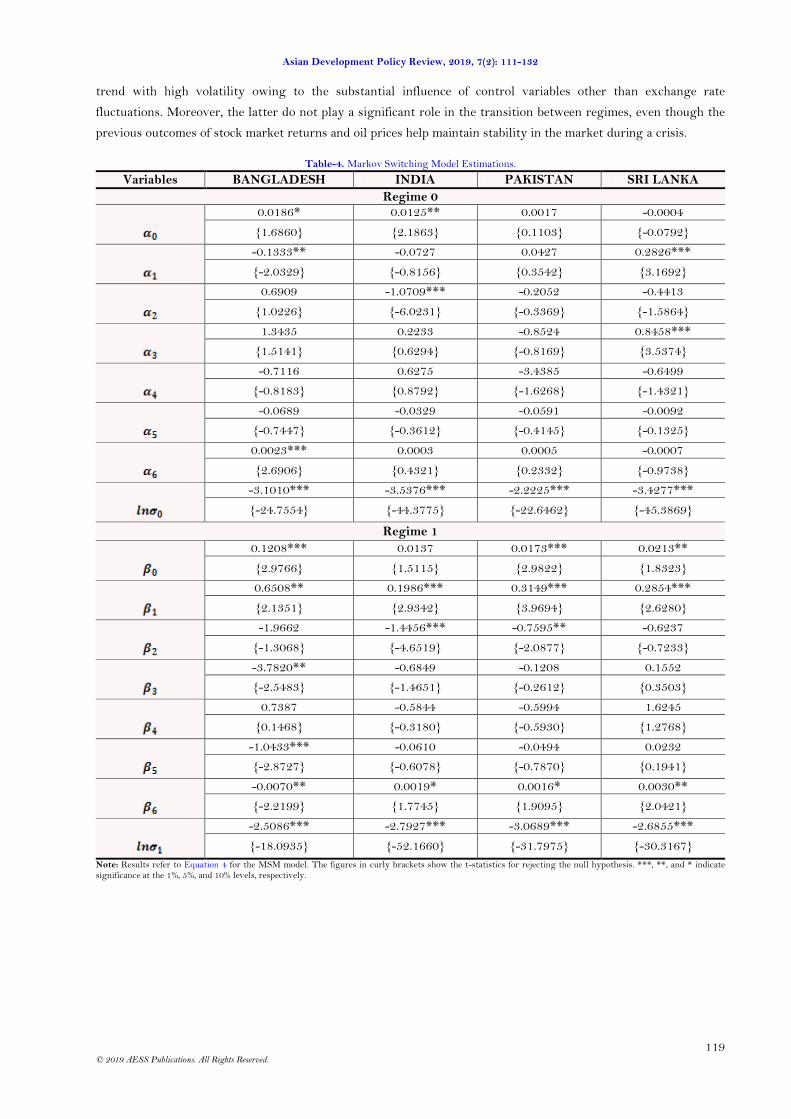
4.2. The Regime-Dependent Relationship between Stock Market and Currency Returns

An investigation was undertaken into whether there are indications of different regimes existing for stock

market returns. The readiness to switch with the data depends on the economic dynamics that lead to a switching

behavior. Empirical estimates of the Markov switching model, along with the means and variances involved, are

shown in Table 4, and the features of the regime are explained in Table 5. The models for each country identified

two regimes (the first referred to as regime/state 0 and the second as regime/state 1) with different volatilities, in

which the effect of exchange rate fluctuations and selected macroeconomic variables on stock market returns differ

substantially.

The analysis revealed that Bangladeshi stock market returns responded to their own lagged market and oil

prices in both the regimes, although the latter had a minor negative impact on the stock market. Furthermore,

inflation and industrial production only exerted approximately 380% and 104% negative impacts on stock market

returns in state 1. Panel A of Table 5 shows that the transition probability of 0.6242 in regime 0 is higher than that

of 0.1048 in regime 1. The significance of these probabilities (P11 and P22) suggests that the low volatility regime is

more persistent than the high one; in other words, the Bangladeshi stock market remained longer in regime 0 than

1, although the market observed high volatility in both regimes. This finding is confirmed by the average duration

(in months) for each regime (d0 and d1) exhibiting low volatility for 2.66 months, due to frequent inconsistencies in

the market. The results of this analysis indicate the dominance of regime 0, which signifies a bearish trend with low

volatility during a crisis in the stock market; however, when there is no crisis, the capital market displays a bullish


119


trend with high volatility owing to the substantial influence of control variables other than exchange rate

fluctuations. Moreover, the latter do not play a significant role in the transition between regimes, even though the

previous outcomes of stock market returns and oil prices help maintain stability in the market during a crisis.

Table-4. Markov Switching Model Estimations.

Variables BANGLADESH INDIA PAKISTAN SRI LANKA

Regime 0

0.0186* 0.0125** 0.0017 -0.0004

{1.6860} {2.1863} {0.1103} {-0.0792}

-0.1333** -0.0727 0.0427 0.2826***

{-2.0329} {-0.8156} {0.3542} {3.1692}

0.6909 -1.0709*** -0.2052 -0.4413

{1.0226} {-6.0231} {-0.3369} {-1.5864}

1.3435 0.2233 -0.8524 0.8458***

{1.5141} {0.6294} {-0.8169} {3.5374}

-0.7116 0.6275 -3.4385 -0.6499

{-0.8183} {0.8792} {-1.6268} {-1.4321}

-0.0689 -0.0329 -0.0591 -0.0092

{-0.7447} {-0.3612} {-0.4145} {-0.1325}

0.0023*** 0.0003 0.0005 -0.0007

{2.6906} {0.4321} {0.2332} {-0.9738}

-3.1010*** -3.5376*** -2.2225*** -3.4277***

{-24.7554} {-44.3775} {-22.6462} {-45.3869}

Regime 1

0.1208*** 0.0137 0.0173*** 0.0213**

{2.9766} {1.5115} {2.9822} {1.8323}

0.6508** 0.1986*** 0.3149*** 0.2854***

{2.1351} {2.9342} {3.9694} {2.6280}

-1.9662 -1.4456*** -0.7595** -0.6237

{-1.3068} {-4.6519} {-2.0877} {-0.7233}

-3.7820** -0.6849 -0.1208 0.1552

{-2.5483} {-1.4651} {-0.2612} {0.3503}

0.7387 -0.5844 -0.5994 1.6245

{0.1468} {-0.3180} {-0.5930} {1.2768}

-1.0433*** -0.0610 -0.0494 0.0232

{-2.8727} {-0.6078} {-0.7870} {0.1941}

-0.0070** 0.0019* 0.0016* 0.0030**

{-2.2199} {1.7745} {1.9095} {2.0421}

-2.5086*** -2.7927*** -3.0689*** -2.6855***

{-18.0935} {-52.1660} {-31.7975} {-30.3167}

Note: Results refer to Equation 4 for the MSM model. The figures in curly brackets show the t-statistics for rejecting the null hypothesis. ***, **, and * indicate significance at the 1%, 5%, and 10% levels, respectively.


120


Table-5. Regime Characteristics of the Markov Switching Model.

Panel A: Regime-Switching Characteristics

Statistics BANGLADESH INDIA PAKISTAN SRI LANKA

Transition Probabilities

Regime 0 Regime 1 Regime

0 Regime

1 Regime 0

Regime 1

Regime 0

Regime 1

Regime 0 0.6242 0.3758 0.9950 0.0050 0.9393 0.0607 0.9526 0.0474 Regime 1 0.8952 0.1048 0.0033 0.9967 0.0280 0.9720 0.0653 0.9347

Expected Duration 2.6610 1.1171 198.3705 300.5724 16.46366 35.73076 21.0870 15.3180

Log Likelihood

Ratio 185.9586 438.7792 359.9949 363.9070

Panel B: Diagnostic Tests

Q(12) 12.5267 (0.4044) 8.3207 (0.6840) 13.3200 (0.3460) 15.7410 (0.2030)

Qs(12) 7.9616 (0.7880) 9.5524 (0.7210) 28.9560*** (0.0040) 3.1605 (0.9940)

J–B 118.5779*** (0.0000) 3.4079 (0.1820) 314.4038*** (0.0000) 7.8646** (0.0196) Note: J–B refers to the Jarque–Bera Normality test. Q(12) and Qs(12) refer to the Box–Pierce serial correlation test for residuals and squared residuals, respectively. The figures in parentheses show the p-values. The expected durations for each regime are d0 and d1. ** and *** indicate statistical significance at the 5% and 1% levels, respectively.

It is noteworthy that the results for India and Pakistan were analogous and revealed very stable economic

conditions: the of the returns reported in Table 4 show that both regime 0 and 1 are experiencing a low volatile

situation. The mean estimates for the lagged stock market returns and crude oil prices in the preceding period also

show a significantly positive response to the stock market returns in regime 1 for both countries. In addition, the

relationship between the stock market and exchange rate returns is significantly negative in regime 1, from which

can be inferred that stock market returns for India and Pakistan dropped by about 144% and 76% in a month,

respectively. Estimations of the transition probabilities for both countries are very close to 1 in both regimes, while

the enormity of P11 and P22 suggests that both regimes are more persistent, or both stock markets remained for

longer periods in each regime, though slightly longer in regime 1. These outcomes are also supported by the

average duration in months for each regime, elucidating stable market attributes. Overall, the Indian and Pakistani

stock markets behaved virtually the same, with the predominance of regime 1 demonstrating a bullish trend with

comparatively low volatility when there is no crisis. Under these conditions, despite fluctuating exchange rates,

lagged stock market returns and oil prices helped stabilize the markets for the long period of time covered by this

study.

The final column of Table 4 provides the estimation results of the MSM model for Sri Lanka, and the mean

estimates for one period of lagged stock market returns were found to be significantly positive for both regimes.

The inflation rate is also significant in regime 0, leading to an 84% improvement, while crude oil prices are

significantly negative in regime 1, with stock market returns declining slightly over one month. Although the Sri

Lankan stock market is persistent in both regimes, the transition probability of being in regime 0 is found to be

comparatively less volatile than remaining in regime 1. This is upheld by the constant average duration in months

for each regime: the low volatile regime 0 lasted 21 months, but the highly volatile regime 1 only lasted around 15

months. Thus, during a crisis, regime 0 prevails as a bear market with low volatility; however, the Sri Lankan stock

market significantly triumphed over bearish trends with low volatility.

4.3. Smooth Transition Probabilities

The smooth transition probabilities derived from the MSM are presented in Figure 1. The MSM captured all

the main highly volatile periods for the selected SAARC countries. Some international crises that affected these

markets include the Asian Financial Crisis (1997–1998) and Global Financial Crisis (2007–2008), with each

suffering local crises as well.


121



122


Figure-1. Transition probabilities.

For Bangladesh (Figure 1a), a smooth transition probability for being in regime 1 was estimated, indicating a

very high range of volatility, while the stock market experienced a bullish trend when no crisis occurred. Stock

market returns, directly affected by exchange rate fluctuations and other control variables, exhibited significant

responses to the financial shocks following the Global Financial Crisis and other occasional local crises. Significant

increases in volatility were first noticed from mid-2005 to the first half of 2007, followed by a series of fluctuations

between 2008 and 2012: the stock market faced a dramatic downturn in 2010 subsequent to the capital market

experiencing abnormal turbulence from around 2005 and ending with the burst of the asset price bubble in 2010.

The main reasons behind such behavior include: the aftereffects from the 1996 collapse, demand induction due to

political conditions since 2007, shortages in the gas and power sector, excess savings, idle business funds, the 2007–

2008 Global Financial Crisis, and surplus liquidity in 2009. The repercussions continued for several years

afterwards. Similarly, another volatile period delivered a series of shocks to the Bangladeshi financial market in

2014–2015 when the country experienced a significant slowdown in business activity due to political disorder and

blockades, and a decline in interest rates. The market recovered in the following year, however, owing to successive

attempts at corrective measures.

Figure 1b illustrates the smooth transition probabilities for India, which are particularly interesting for regime

1. There was a very long period, from 1993 to 2008, without any crises; this low volatility preceded a single market

deviation only during the Global Financial Crisis, followed by a long-term crisis. Since 1992, India has experienced

two incidences of considerable stock market growth, in 1992–1993 and 1999–2000. The first expansion reflected

price deregulation driven by a liberal monetary policy; however, investors realized stock prices were overvalued in

the primary market, public confidence in the equity market declined following a series of scams and malpractice

during 1992 and 1993, the inflow of foreign capital reduced following the Mexican and South Asian crises, and the

impact of several global phenomena was felt, resulting in a decline in equity finance up to 1999. In that year, the

stock market expanded again on account of the IT boom and a reduction in capital gains tax. As the Indian

economy is mainly an open one, the Indian financial market as a whole suffered a depression in 2008–2009. The

stock market has experienced huge drops, and its highest ever loss, as weak global signals have created panic

among investors, who fear a dramatic slump in US markets. Several factors lie behind this decline: changing the

global investment environment, fear of recession in the US economy, global credit crisis and distress, sale of foreign

hedge funds to enable reallocation from uncertain emerging markets to stable developed markets, cuts in US

interest rates, volatility in the commodities markets, and several other influences from local factors. Consequently,

from 2009 onwards, the Indian stock market experienced a depression.

The smooth transition probabilities for Pakistan (Figure 1c) indicates that the market frequently vacillated in

high and low volatile regimes. As Pakistan is a partially open economy, the market reacted to financial shocks from

internal crises in the main, but the Asian and Global Financial Crises as well. A significant increase in volatility was


123


observed from 1994 to mid-2000, leading to a bearish trend in the market. It involved the collapse of the equity

market in 1995, caused by the domestic political crisis and a discouraging macroeconomic outlook, and the

devaluation of the Pakistani rupee in October 1997. Then, in 1998, the local capital market suffered a violent crash

in the face of such events as the South East Asian financial collapse and global recession. Similarly, the financial

shock from the subprime mortgage crisis and major related economic failures also affected Pakistan between 2007

and 2009, which explains the market’s transition to a highly volatile regime. Major macroeconomic factors during

that period include: the Red Mosque incident, terrorism, reaction to the 2007 Karsaz bombing during the reception

for Mrs. Benazir Bhutto on October 18, declaration of a state of emergency, suspension of Pakistan from the

Commonwealth, and assassination of Mrs. Benazir Bhutto on December 27, 2007, which resulted in the largest

crash of the financial market. As it is evident that Pakistan's stock market returns are closely linked to

macroeconomic variables and the business cycle, the remaining highly volatile periods can be rationally attributed

to country-specific affairs and risk factors.

The smooth transition probabilities of Sri Lanka being in regime 1 (Figure 1d) suggest that over the period of

the study, the market frequently vacillated between high and low volatility. Troughs in the graph illustrate

comparatively low volatile crisis trends in the Sri Lankan economy; specifically, the first downturn in the stock

market occurred between June 1999 and 2001, indicating the effects of the civil war (Eelam War III), Asian

Financial Crisis (1997–1998), and other global events. Another crisis occurred between August 2006 and May 2008,

during which time the ceasefire agreement between the Sri Lankan and internal guerilla leaders ended, along with

the associated positive political attributes and economic developments, despite the existence of rigid forces, which in

turn led to slower growth in the CSE Index. A further two periods of the crisis were observed throughout the

2010s. First, the formidable economic expansion after the civil war ended on May 19, 2009, diminished under the

uncertainty in the global markets and domestic market issues (i.e., a series of tighter regulations, stringent trading

measures for market insiders, and a high interest rate environment), which disrupted stock market performance.

Second, the crisis between late 2013 and 2016 coincided with a decline in the stock market due to a marginal

increase in domestic interest rates, political uncertainty, depreciation of the domestic exchange rate, global factors,

declining commodity prices, and a drop in oil prices.

Overall, the Indian and Pakistani stock markets were relatively more consistent in regime 1, when there were

no crises, and experienced a bullish trend in market performance. In contrast, the capital markets of Bangladesh and

Sri Lanka were the least volatile in regime 0, during a crisis, and inclined toward bearish market behavior. These

outcomes imply that these stock markets are characterized by a state in which risk is relatively low and investors

earn more than when retaining liquidity funds, while they lose money in a state in which risk is substantially

higher. These results are consistent with the findings of Kanas (2005) and Chan et al. (2011). For instance, Kanas

(2005) provides evidence of two regimes in the relationship between the Mexican exchange rate and the stock

market returns of some emerging countries. Moreover, the results obtained by Kanas (2005) indicate that a low

volatility regime is more persistent than a highly volatile one.

An obvious question is whether there is still evidence that stock market returns can be predicted using

macroeconomic variables, after switching control. Fads models4 provide one possible economic motivation for

Markov switching processes: stock market returns are predictable.5 The predictability of returns can also stem from

time variations in the risk premium of an efficient market,6 while their nonlinear predictability could arise as a result

4 Fads are any form of collective behavior that often appears suddenly, quickly spreads, is short-lived, and then fades; this is different from trends

that develop slowly and last longer. In the main, fads are represented in the model by peaks that generate and deteriorate rapidly.

5 In a context with fads, Schaller and Norden (1997) demonstrated that returns were correlated with lagged values of the price/dividend ratio,

while Chkili and Nguyen (2014) and Sarafrazi et al., (2015) revealed the correlation between stock market returns and exchange rate fluctuations.

6 See Fama (1990, 1991) for further discussion.


124


of the kind of stochastic bubbles proposed by Blanchard and Watson (1982). In this study, the empirical estimations

for all the markets provided strong evidence of predictability, indicating that the Indian and Pakistani stock market

returns are mainly predicted by exchange rate fluctuations, and through other macroeconomic variables for

Bangladesh and Sri Lanka.

On the whole, the results of the time-varying MSM models for all the selected countries show that only the

Indian and Pakistani stock market returns are negatively influenced by fluctuations in their exchange rates during

bull cycles when there are no crises. This significant negative relationship between the stock market and currency

returns suggests that equity markets are likely to respond to foreign exchange devaluation with a decrease in prices

accompanied by an increase in the required risk premium. For Bangladesh and Sri Lanka, the results corroborate

those of previous studies (e.g.Kanas, 2000; Yang and Doong, 2004; Chkili and Nguyen, 2014), suggesting that

fluctuations in currency returns exert little effect on stock market return dynamics. For example, Kanas (2000)

examined the volatility spillover between exchange rates and stock markets in some developed countries and

reported that the transmission of volatility from foreign exchange markets to stock markets was insignificant for all

the countries selected. Likewise, Yang and Doong (2004) produced similar results for the G7 countries, stating that

fluctuations in exchange rates have less of a direct impact on future stock price changes; this can be explained by

means of effective hedging strategies against currency risks through available currency derivatives. Furthermore,

Chkili and Nguyen (2014) found that significant impacts from exchange rates only occurred in BRICS countries.

Conversely, a single period of lagged stock market returns and crude oil prices were found to be important

control variables that influenced the bear and bull cycles in all the stock markets. Yıldırım et al. (2018) estimated

that in all countries the response of the stock market to an unexpected oil price shock is positive and statistically

significant in highly volatile regimes, suggesting that oil price increases can be estimated by demand-side shock. Sri

Lankan stock market returns were further influenced positively by the inflation rate during a bear trend, due to its

long civil war, which is in line with Fisher’s (1930) prediction of a positive relationship between expected inflation

and nominal asset returns. In addition, major constraints were found on Bangladesh's stock market and industrial

production growth, which had a negative impact on bull markets, mainly because of demand-side shocks leading to

price bubbles on the market during a regime without crises; otherwise, at such times, inflation has no impact on

stock market returns (Hondroyiannis and Papapetrou, 2006).

5. CONCLUSION AND POLICY IMPLICATIONS

The evidence of switching behavior in stock market returns is provided by both means and variances. By

applying a test amended from an earlier study by Schaller and Norden (1997), switching is shown to be much

stronger in all the markets during a crisis. This research also examined investors' insight into foreign exchange risk

on the SAARC stock markets. Regime-switching models substantiated nonlinearities in the link between exchange

rate fluctuation and equity returns; in particular, the Markov switching dynamic factor model detected regime shifts

in the stock market returns as a result of currency returns and other macroeconomic factors and found evidence of

two distinct regimes with low and high volatility in each SAARC country. This study revealed the regime-

dependent effect of exchange rate fluctuations on stock market returns in India and Pakistan. However, fluctuations

in the equity markets in Bangladesh and Sri Lanka were affected more by domestic crises and, despite being just as

regime-dependent, by other macroeconomic factors that appeared from time to time in the market.

The inferred probabilities and average regime durations indicated that market switching varied across the

selected countries. The Indian market switched regimes only once over the period studied; by comparison, the

Pakistani and Sri Lankan markets switched more frequently; meanwhile, the Bangladeshi stock market switched

much more sharply between the two regimes—owing to their crises being multiple random events rather than

based on a priori dates or structural changes occurring locally—after the onset of local and international financial


125


crises. An increased frequency of regime switching indicates greater uncertainty and a strong tendency toward

higher volatility of equity returns during both calm and turbulent regimes.

Evidence for the prediction of regimes was found for all the selected countries. Although both regimes/states

were highly persistent in India and Pakistan, and the asymmetric effects of substantial currency depreciation

occurred in state 1, casual empiricism suggests that controlled devaluation may eventually be overtaken by market

forces, driven either by game-theoretic rounds of further devaluation or by the shifting focus of risk-averse global

investors across financial markets. However, interest rates, inflation, and industrial production growth were shown

to be insignificant to any change in returns, while the market performance and crude oil prices in the preceding

period could be positive for stock market returns during a calm regime; therefore, both stock markets were

progressing well but with a declining tendency. Similarly, both states were highly persistent in Sri Lanka, with

some exceptions during turbulent regimes when there were high rates of inflation due to the onset of civil war,

hindering the stock market. In contrast, the Bangladeshi stock market was quite unstable during both regimes, with

the suggestion that since the market was largely affected by long-term demand-side shocks in a calm regime, the

effects of inflation and oil prices, apart from industrial production growth, would increase investors' hesitancy in the

equity market as well as the likelihood of financial distress and insolvency. This could not be easily dismissed, at

least not until the government had implemented strict measures to control those shocks.

In light of the empirical evidence in this study, it is asserted that regime switching in the stock markets of each

SAARC country is influenced by both internal and external economic, financial, and political conditions.

Policymakers should thus be aware that financial shocks can have considerable real impacts, as proved by not only

the recent Global Financial Crisis but also many other domestic crises. Furthermore, when developing an optimal

strategy to preserve financial stability in the event of a crisis, those in Pakistan and India should also take note that

these shocks are transmitted between foreign exchange and stock markets. Finally, our empirical findings will also

assist the central banks of the respective SAARC countries with monetary policies and regulations, and exchange

rate regimes. Stock market returns have been studied so extensively that it often seems that very little can be added

to the existing knowledge; however, by extending the techniques and findings of Hamilton (1989) and Schaller and

Norden (1997), this study does highlight several features of improvement for stock market performance. In

conclusion, the authors invite both other empirical researchers to utilize these outcomes and asset pricing theorists

to attempt to account for the stylized facts that emerged from this study.

Funding: This study received no specific financial support. Competing Interests: The authors declare that they have no competing interests. Contributors/Acknowledgement: This paper is part of a Ph.D. dissertation. The authors wish to express their immense appreciation for the guidance and frequent assistance provided by Dr. Waliullah of the Institute of Business Administration, Karachi, in the pursuance of suitable econometric techniques.

REFERENCES

Andreopoulos, S., 2009. Oil matters: Real input prices and US unemployment revisited. The BE Journal of Macroeconomics,

9(1): 1-31.Available at: https://doi.org/10.2202/1935-1690.1632.

Ang, A. and G. Bekaert, 1999. International asset allocation with time-varying correlations (No. w7056). National Bureau of

Economic Research.

Balcilar, M., R. Gupta and S.M. Miller, 2015. Regime switching model of US crude oil and stock market prices: 1859 to 2013.

Energy Economics, 49: 317-327.Available at: https://doi.org/10.1016/j.eneco.2015.01.026.

Blanchard, O.J. and M. Watson, 1982. Bubbles, rational expectations and financial markets, in crises in the economic and

financial structure. Ed. P. Watchel. Lexington MA: Lexington Books.

Cecchetti, S.G., P.S. Lam and N.C. Mark, 1990. Mean reversion in equilibrium asset prices. American Economic Review, 80(3):

398-418.


126


Chan, K.F., S. Treepongkaruna, R. Brooks and S. Gray, 2011. Asset market linkages: Evidence from financial, commodity and

real estate assets. Journal of Banking & Finance, 35(6): 1415-1426.Available at:

https://doi.org/10.1016/j.jbankfin.2010.10.022.

Chkili, W., A. Chaker, O. Masood and J. Fry, 2011. Stock market volatility and exchange rates in emerging countries: A

Markov-state switching approach. Emerging Markets Review, 12(3): 272-292.Available at:

https://doi.org/10.1016/j.ememar.2011.04.003.

Chkili, W. and D.K. Nguyen, 2011. Modeling the volatility of mediterranean stock markets: A regime-switching approach.

Economic Bulletin, 31(2): 1-9.

Chkili, W. and D.K. Nguyen, 2014. Exchange rate movements and stock market returns in a regime-switching environment:

Evidence for BRICS countries. Research in International Business and Finance, 31(C): 46-56.Available at:

https://doi.org/10.1016/j.ribaf.2013.11.007.

Davies, R.B., 1987. Hypothesis testing when a nuisance parameter is present only under the alternative. Biometrika, 74(1): 33-

43.Available at: https://doi.org/10.1093/biomet/74.1.33.

Ehrmann, M., M. Ellison and N. Valla, 2003. Regime-dependent impulse response functions in a Markov-switching vector

autoregression model. Economics Letters, 78(3): 295-299.Available at: https://doi.org/10.1016/s0165-1765(02)00256-

2.

Fama, E.F., 1990. Stock returns, expected returns, and real activity. The Journal of Finance, 45(4): 1089-1108.Available at:

https://doi.org/10.1111/j.1540-6261.1990.tb02428.x.

Fama, E.F., 1991. Efficient capital markets: II. The Journal of Finance, 46(5): 1575-1617.Available at:

https://doi.org/10.1111/j.1540-6261.1991.tb04636.x.

Fisher, I., 1930. Theory of interest: As determined by impatience to spend income and opportunity to invest it. Clifton:

Augustusm Kelly Publishers.

Flavin, T.J., E. Panopoulou and D. Unalmis, 2008. On the stability of domestic financial market linkages in the presence of time-

varying volatility. Emerging Markets Review, 9(4): 280-301.Available at:

https://doi.org/10.1016/j.ememar.2008.10.002.

Garcia, R., 1998. Asymptotic null distribution of the likelihood ratio test in Markov switching models. International Economic

Review, 39(3): 763-788.Available at: https://doi.org/10.2307/2527399.

Garcia, R. and P. Perron, 1996. An analysis of the real interest rate under regime shifts. The Review of Economics and Statistics,

78(1): 111-125.Available at: https://doi.org/10.2307/2109851.

Goldfeld, S.M. and R.E. Quandt, 1973. A Markov model for switching regressions. Journal of Econometrics, 1(1): 3-15.Available

at: https://doi.org/10.1016/0304-4076(73)90002-x.

Granger, C.W., 1996. Can we improve the perceived quality of economic forecasts? Journal of Applied Econometrics, 11(5): 455-

473.Available at: https://doi.org/10.1002/(sici)1099-1255(199609)11:5<455::aid-jae408>3.3.co;2-5.

Hamilton, J., 1989. A new approach to the economic analysis of nonstationary time series and the business cycle. Econometrica ,

57(2): 357-384.Available at: https://doi.org/10.2307/1912559.

Hamilton, J.D. and R. Susmel, 1994. Autoregressive conditional heteroskedasticity and changes in regime. Journal of

Econometrics, 64(1-2): 307-333.Available at: https://doi.org/10.1016/0304-4076(94)90067-1.

Hansen, B.E., 1992. The likelihood ratio test under nonstandard conditions: Testing the Markov switching model of GNP.

Journal of Applied Econometrics, 7(S1): S61-S82.Available at: https://doi.org/10.1002/jae.3950070506.

Hansen, B.E., 1993. Inference when a nuisance parameter is not identified under the null hypothesis. Mimeo: University of

Rochester.

Hansen, B.E., 2001. The new econometrics of structural change: Dating breaks in US labour productivity. Journal of Economic

Perspectives, 15(4): 117-128.Available at: https://doi.org/10.1257/jep.15.4.117.


127


Holmes, M.J. and M. Nabil, 2002. Non-linearities, regime switching and the relationship between Asian equity and foreign

exchange markets. International Economic Journal, 16(4): 121-139.Available at:

https://doi.org/10.1080/10168730200000032.

Hondroyiannis, G. and E. Papapetrou, 2006. Stock returns and inflation in Greece: A Markov switching approach. Review of

Financial Economics, 15(1): 76-94.Available at: https://doi.org/10.1016/j.rfe.2005.02.002.

Ismail, M.T. and Z. Isa, 2008. Identifying regime shifts in Malaysian stock market returns. International Research Journal of

Finance and Economics, 15(1): 36-49.

Kanas, A., 2000. Volatility spillovers between stock returns and exchange rate changes: International evidence. Journal of

Business Finance & Accounting, 27(3-4): 447-467.Available at: https://doi.org/10.1111/1468-5957.00320.

Kanas, A., 2005. Regime linkages between the Mexican currency market and emerging equity markets. Economic Modelling,

22(1): 109-125.Available at: https://doi.org/10.1016/j.econmod.2004.05.003.

Kim, C.J. and C.R. Nelson, 1999. State space models with regime switching, classical and gibbs sampling approaches with

applications. Cambridge, MA: MIT Press.

Krolzig, H.M., 1997. Markov switching autoregressive: Modeling statistical inference and application to business cycles analysis.

Berlin: Springer.

Moore, T. and P. Wang, 2007. Volatility in stock returns for new EU member states: Markov regime switching model.

International Review of Financial Analysis, 16(3): 282-292.Available at: https://doi.org/10.1016/j.irfa.2007.03.006.

Perron, P., 2006. Dealing with structural breaks. Palgrave Handbook of Econometrics, 1(2): 278-352.

Qiao, Z., Y. Li and W.-K. Wong, 2011. Regime-dependent relationships among the stock markets of the US, Australia and New

Zealand: a Markov-switching VAR approach. Applied Financial Economics, 21(24): 1831-1841.Available at:

https://doi.org/10.1080/09603107.2011.595678.

Rydén, T., T. Teräsvirta and S. Åsbrink, 1998. Stylized facts of daily return series and the hidden Markov model. Journal of

Applied Econometrics, 13(3): 217-244.Available at: https://doi.org/10.1002/(sici)1099-

1255(199805/06)13:3<217::aid-jae476>3.0.co;2-v.

Sarafrazi, S., S. Hammoudeh and M. Balcilar, 2015. Interactions between real economic and financial sides of the US economy in

a regime-switching environment. Applied Economics, 47(60): 6493-6518.Available at:

https://doi.org/10.1080/00036846.2015.1080806.

Schaller, H. and S.V. Norden, 1997. Regime switching in stock market returns. Applied Financial Economics, 7(2): 177-

191.Available at: https://doi.org/10.1080/096031097333745.

Schwert, G.W., 1989. Why does stock market volatility change over time? The Journal of Finance, 44(5): 1115-1153.Available

at: https://doi.org/10.1111/j.1540-6261.1989.tb02647.x.

Semmler, W. and P. Chen, 2014. Financial stress, regime switching and macrodynamics: Theory and empirics for the US, the

EU and non-EU countries. Economics: The Open-Access, Open-Assessment E-Journal, 8(2014-20): 1-42.Available at:

https://doi.org/10.5018/economics-ejournal.ja.2014-20.

Timmermann, A., 2000. Moments of Markov switching models. Journal of Econometrics, 96(1): 75-111.Available at:

https://doi.org/10.1016/s0304-4076(99)00051-2.

Turner, C.M., R. Startz and C.R. Nelson, 1989. A markov model of heteroskedasticity, risk, and learning in the stock market.

Journal of Financial Economics, 25(1): 3-22.Available at: https://doi.org/10.1016/0304-405x(89)90094-9.

Wang, P. and M. Theobald, 2008. Regime-switching volatility of six East Asian emerging markets. Research in International

Business and Finance, 22(3): 267-283.Available at: https://doi.org/10.1016/j.ribaf.2007.07.001.

Yang, S.-Y. and S.-C. Doong, 2004. Price and volatility spillovers between stock prices and exchange rates: Empirical evidence

from the G-7 countries. International Journal of Business and Economics, 3(2): 139-153.

Yıldırım, D.Ç., S. Erdoğan and E.İ. Çevik, 2018. Regime-dependent effect of crude oil price on BRICS stock markets. Emerging

Markets Finance and Trade, 54(8): 1706-1719.Available at: https://doi.org/10.1080/1540496x.2018.1427062.


128


Appendix-A. Bangladeshi Financial Markets

Figure-1. Trend charts of Bangladeshi financial market and macroeconomic factors, overall sample size ranges for a monthly period ranging from January 2005 to December 2016.

Source: Data on stock prices from Central Bank of Bangladesh, exchange rates are from www.oanda.com, and rest from International Monetary Fund.


129


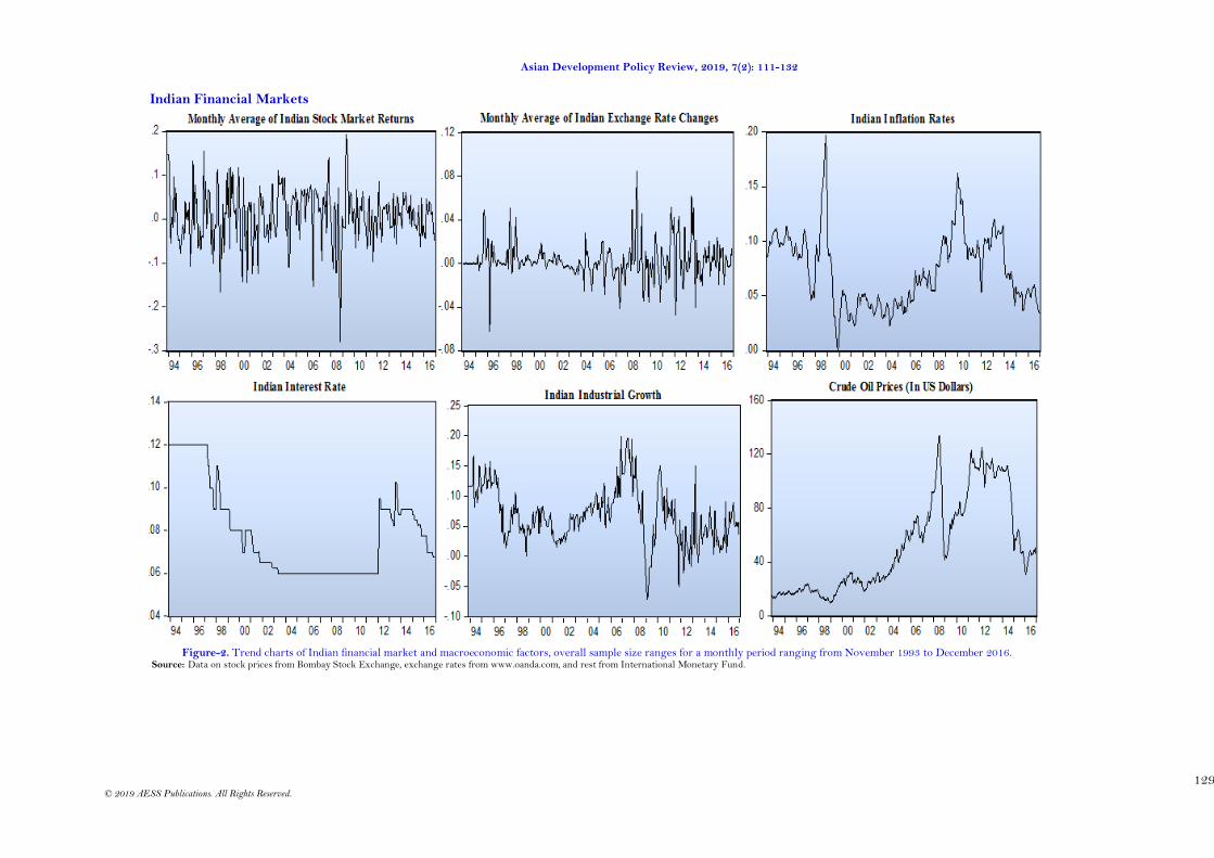
Indian Financial Markets

Figure-2. Trend charts of Indian financial market and macroeconomic factors, overall sample size ranges for a monthly period ranging from November 1993 to December 2016.

Source: Data on stock prices from Bombay Stock Exchange, exchange rates from www.oanda.com, and rest from International Monetary Fund.


130


Pakistani Financial Markets

Figure-3. Trend charts of Pakistani financial market and macroeconomic factors, overall sample size ranges for a monthly period ranging from November 1993 to December 2016.

Source: Data on stock prices from State Bank of Pakistan, exchange rates are from www.oanda.com, and rest from International Monetary Fund.


131


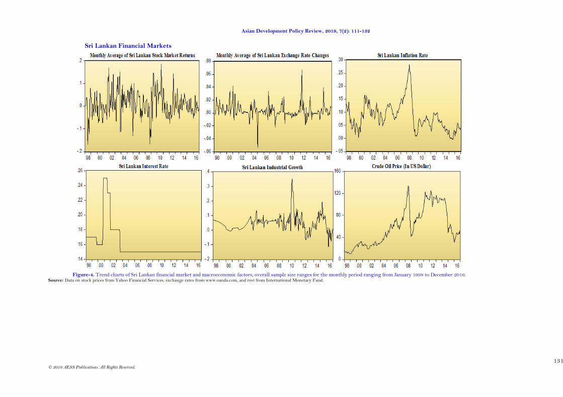
Sri Lankan Financial Markets

Figure-4. Trend charts of Sri Lankan financial market and macroeconomic factors, overall sample size ranges for the monthly period ranging from January 1998 to December 2016.

Source: Data on stock prices from Yahoo Financial Services, exchange rates from www.oanda.com, and rest from International Monetary Fund.


132


Appendix-B. Scatter Plots for Analysis of Nonlinearity in the Model

Bangladesh India Pakistan Sri Lanka

Views and opinions expressed in this article are the views and opinions of the author(s), Asian Development Policy Review shall not be responsible or answerable for any loss, damage or liability etc. caused in relation to/arising out of the use of the content.

Asian Development Policy Revie2)-111-132.pdfThis study conducts a joint evaluation of nonlinear...

Documents

Transcript of Asian Development Policy Revie2)-111-132.pdfThis study conducts a joint evaluation of nonlinear...