Asian Development Bank Institute paper is organized as follows. First, evidence on urban...

ADBI Working Paper Series

COSTS AND BENEFITS OF URBANIZATION: THE INDIAN CASE

Kala Seetharam Sridhar

No. 607 October 2016

Asian Development Bank Institute

The Working Paper series is a continuation of the formerly named Discussion Paper series; the numbering of the papers continued without interruption or change. ADBI’s working papers reflect initial ideas on a topic and are posted online for discussion. ADBI encourages readers to post their comments on the main page for each working paper (given in the citation below). Some working papers may develop into other forms of publication.

Suggested citation:

Sridhar , K.S. 2016. Costs and Benefits of Urbanization: The Indian Case. ADBI Working Paper 607. Tokyo: Asian Development Bank Institute. Available: https://www.adb.org/publications/costs-and-benefits-urbanization-indian-case Please contact the author for information about this paper.

Email: [email protected] [email protected] [email protected]

Kala Seetharam Sridhar is a professor at the Centre for Research in Urban Affairs at the Institute for Social and Economic Change in Bangalore, India. The views expressed in this paper are the views of the author and do not necessarily reflect the views or policies of ADBI, ADB, its Board of Directors, or the governments they represent. ADBI does not guarantee the accuracy of the data included in this paper and accepts no responsibility for any consequences of their use. Terminology used may not necessarily be consistent with ADB official terms. Working papers are subject to formal revision and correction before they are finalized and considered published.

Asian Development Bank Institute Kasumigaseki Building 8F 3-2-5 Kasumigaseki, Chiyoda-ku Tokyo 100-6008, Japan Tel: +81-3-3593-5500 Fax: +81-3-3593-5571 URL: www.adbi.org E-mail: [email protected] © 2016 Asian Development Bank Institute

ADBI Working Paper 607 Sridhar Abstract Urbanization has both benefits and costs. In a market economy, the trade-off between benefits and costs determines the level, speed, and pace of urbanization. This paper summarizes research findings on how urbanization enhances productivity and economic growth in both rural and urban sectors, taking the case of India. We study the relationship between urbanization and growth in the Indian context by examining microeconomic evidence on how enterprises and consumers share production and infrastructure costs, match with specialized workers and employers more efficiently in the labor market, and learn from other producers and workers. Based on extensive data analyses of urbanization, we find no impact of urban–rural inequalities on urbanization, but a significant impact on the population of the largest city in the state. When accounting for the two-way relationship between urbanization and the rural–urban income ratio, we find that urbanization increases urban–rural inequalities initially, but, at higher levels, reduces them. This paper also studies how the urban areas are affected by migration from rural areas and how rural areas benefit from urban development. Furthermore, policy implications regarding telecommuting and investments in urban infrastructure are summarized. Lessons from India and the People’s Republic of China for each other’s urbanization are also discussed. JEL Classification: R12, O18, O57

ADBI Working Paper 607 Sridhar Contents

1. Introduction and Scope .............................................................................................. 1

2. Evidence on Urban Agglomeration Economies and Economic Growth ...................... 1

3. Sharing, Matching, and Learning ............................................................................... 7

4. Urbanization: Level, Speed, and Regional Variation .................................................. 7

5. Regional Variation ................................................................................................... 11

6. The Urbanization–Industrialization Gap ................................................................... 12

7. Benefits and Costs of Urbanization: Analytical Framework ...................................... 13

8. Data and Sources .................................................................................................... 14

9. Empirical Results ..................................................................................................... 15

10. Results from Regressions ........................................................................................ 20

11. Rural Employment and Remittances ........................................................................ 23

12. Policy Implications ................................................................................................... 26

References ......................................................................................................................... 29

ADBI Working Paper 607 Sridhar

1. INTRODUCTION AND SCOPE Urbanization has both benefits and costs. In a market economy, the trade-off between benefits and costs determines the level, speed, and pace of urbanization. In this paper, we summarize research findings on how urbanization enhances productivity and economic growth in both rural and urban sectors. Using the Indian context, we examine the microeconomic evidence on how enterprises and consumers share production and infrastructure costs, match with specialized workers and employers more efficiently in the labor market, and learn from other producers and workers. We study the relationship between urbanization and growth, using data from India. Given urbanization cannot be viewed in isolation, we also study how the urban areas are affected by migration from rural areas and how rural areas, in turn, benefit from urbanization in terms of remittances made by urban migrants to their homes. This paper is organized as follows. First, evidence on urban agglomeration economies and economic growth, growth and productivity, and sharing, matching, and learning is briefly discussed, within each section first internationally and then in terms of evidence from the Indian context. Following that, the level, speed, and regional variation in urbanization for India are described. The urbanization–industrialization gap in the Indian context is summarized, followed by a presentation of the empirical findings with respect to urbanization, which is dependent on benefits and costs. Urbanization cannot be viewed in isolation; hence, the subsequent section then focuses on rural development in India’s context, taking the case of the Mahatma Gandhi National Rural Employment Guarantee Scheme (MGNREGS), whose objective is to arrest rural–urban migration by alleviating rural poverty. In this section, some evidence on remittances by urban migrants to rural areas is summarized. Last, the policy implications of the research are summarized.

2. EVIDENCE ON URBAN AGGLOMERATION ECONOMIES AND ECONOMIC GROWTH

While much of the literature on urbanization in different parts of the world focuses on the relationship between urbanization and growth (Henderson 2004; Krugman 1995; Zhang 2002; Lanaspa, Pueyo, and Sanz 2005; Bertinelli and Strobl 2007; Sridhar and Sridhar 2007; Gilbert and Gugler 1982; McGee 1971), the causes of urbanization are less well studied, especially in the framework of benefits and costs. Henderson (2004) gives credence to this. Brueckner (1990) studies urbanization in the cross-national context within a benefits–costs framework. Theories that are adequate to describe urbanization in Europe and North America are not necessarily applicable to the developing cities of Asia. This lends additional support to investigating the question as to whether the causes of urbanization for Indian states are different from those for the developed world. There is also evidence from Zhang (2002) and Henderson (2004) that the causal link runs from economic growth to urbanization and not vice versa.

Growth and Productivity What do we know about the relationship between urbanization and economic growth in India? Urbanization enhances economic growth. At the global level, the urbanization rate and gross domestic product (GDP) per capita are positively related, but the position of India is below the average level when compared with that of other countries,

1


which means India’s urbanization at 31% lags behind its development stage (with a per capita GDP of $1,503) by about 10 percentage points (Figure 1). One reason why this has occurred is because of the Government of India’s inadequate attention to urbanization and its problems for a long time since independence. India was believed to live primarily in its villages. There is surplus labor in India’s rural areas, which, however, has usually been absorbed by the services sector in the urban areas as Sridhar and Reddy (2014) find with respect to the poor in Bangalore. Paul et al. (2012) and Sridhar and Kashyap (2014) also confirm that services account for the employment of most of India’s urban labor force, clarifying that most Indian cities bypassed the classic transfer of surplus labor from agriculture to manufacturing as demonstrated by the Lewis model and the transition to urbanization.

Figure 1: Relationship between Global Urbanization and GDP per Capita in 2012

CI = confidence interval, GDP = gross domestic product. Source: Data are from the 2012 urbanization rate and GDP per capita in the World Bank database. Liechtenstein and Monaco as outliers as well as Hong Kong, China; Macau, China; Singapore; Taipei,China; Vatican City; Malta; Di San Marino; and the Maldives have been eliminated.

Among other reasons that India is less urban than what is suggested by the country’s level of income is that successive governments (save the current one) have been pessimistic about urbanization, being guided by Todaro’s (1969) model, which suggested that urban areas that increase job opportunities will attract greater migration from rural to urban areas, which would, in turn, paradoxically increase their unemployment rate. This model provided a negative view of urbanization since it implied that no matter what urban areas did, it would be futile to improve their livability. While empirical evidence supporting Todaro’s model has been limited, even using data from India, urban development policies have implicitly been guided by such a model for a long time. For this reason, it was believed that rural–urban migration has to be “checked” as may be seen in the case of programs such as the MGNREGS, which is discussed at the end of this paper. Mills and Becker (1986) point out how, even historically, several policies and programs were in place to “control” urbanization and city size in India. While there is no single document that describes the government’s policies on city size, as they point out, the earliest national government programs to influence the location of industry made use of

2


industrial licenses. In 1977, it was decided that industrial licenses would be denied in large metropolitan areas and urban agglomerations. In addition, direct investment in government-owned enterprises was another means through which the Government of India restricted the growth of large cities. Preference for the location of government-owned industry was given to low-income areas, rural areas, or small cities and towns. Further, according to Mills and Becker (1986), which referred to government encouragement of small-scale industry to locate in small towns and rural areas, a locational program was yet another tool used to control city size. Under these locational programs, a large number of specific instruments such as concessionary finance, input allocations, technical and marketing assistance, training programs, and the development of industrial estates were provided to small industries. A final locational program of the national government, also provided by state governments, was to develop “backward” districts with tools such as subsidies for capital investment, transport subsidy, income tax concessions, and concessional loans. Thus, programs and policies of the Government of India have tried to limit the size and growth of large cities and urbanization by dispersing the location of industry from large cities to smaller towns and rural areas or to poorer states and districts. Despite such policies to “control” urbanization and city size in India, within the country, urbanization is positively related to economic development, measured by average wage and urbanization at the state level (Figure 2).

Figure 2: Relationship between Urbanization and Income, Indian States

Notes: The chart shows the relationship between the urbanization rate and average daily earnings of all employees in the Indian states. All employees include directly employed workers, contract workers, supervisors, managers, and other staff for 2009–2010. Urbanization data are projected for 2009, based on the Census of India data on urbanization for the Indian states for 2001 and 2011. The daily earnings data are in Indian rupees. Sources: Datanet India (www.indiastat.com) for average daily earnings (2009–2010) and Census of India 2011 for urbanization.

Given the policies and programs to control city size, what is the evidence from India regarding Zipf’s law? As Gabaix (1999) points out, Zipf’s law is the most consistent empirical regularity that characterizes the cities of most countries—the United States (US) in 1790 and India in 1911. He also argues that Zipf’s law is a prerequisite for local growth to occur. Zipf’s law has been studied by Basu and Bandyapadhyay (2009) in the context of the size distribution of Indian cities, using data from the Indian censuses of 1981, 1991,

3

http://www.indiastat.com/


and 2001. Their analysis showed that the population distribution in Indian cities does follow a power law similar to the ones found in other countries.1 Mathur (forthcoming) estimates Zipf’s law for Indian cities and finds that large Indian cities are not big enough and the smaller ones are too small, indicated by the rank–size rule, while finding that there is considerable variation in the degree of primacy across Indian states. For instance, Mathur (forthcoming) finds that states such as Karnataka and Tamil Nadu have primate cities, with their capital cities Bangalore and Chennai being several times larger than the second-ranked cities (Mysore and Coimbatore, respectively) in these states, in a manner that does not conform to Zipf’s law. Duranton and Puga (2003) study mechanisms that provide the microeconomic foundations of urban agglomeration economies. They distinguish three types of microfoundations, based on sharing, matching, and learning mechanisms. They do this first by understanding the reasons for the existence of cities. Brueckner (2011) highlights the importance of scale economies and agglomeration economies, respectively, as causes for the existence of factory towns and large cities. To justify the existence of cities, a simple argument is to invoke the existence of indivisibilities in the provision of certain goods or facilities. It is clear that there is a trade-off between the gains from sharing the fixed cost of the facility among a larger number of consumers and the costs of increasingly crowding the land around the facility (e.g., because of road congestion). We may think of a city as the equilibrium outcome of such a trade-off. Cities facilitate the sharing of many indivisible public goods, production facilities, and marketplaces. Duranton and Puga (2003) first conclude that different microeconomic foundations may be used to justify the existence of cities. Second, they find that heterogeneity (of workers and firms) is at the root of most, if not all, mechanisms that underlie the existence of cities. They find that interactions within an “army of clones” could hardly generate sufficient benefits to justify the existence of modern cities. Third, incomplete information often plays a crucial role. Cities make it easier to find inputs (be it workers or intermediate goods) and customers to experiment and discover new possibilities. Fourth, due to the foregoing reasons, sharing and matching mechanisms are well developed. However, the microfoundations of learning mechanisms, especially of knowledge spillovers, are far less satisfactory. Given the importance that such spillovers appear to play in our perception not only of cities but also of growth and innovation, better and more microfounded models of learning and spillovers ought to be an important priority for research in this area. We also know much more about the sources of agglomeration economies at the level of cities (or for that matter, at the level of regions) than at smaller spatial scales. As in other countries, India’s urbanization also serves as the impetus for agglomeration economies, improving employment opportunities and income level (Figure 2). The trend line fitted to the data from Indian states in the figure shows that there is a positive relationship between urbanization and the average daily earnings of employees (directly employed, contract, supervisory, managerial, and other). We expect such a relationship because urbanization enhances productivity, attracts more talented workers, and encourages innovation. However, as the Institute for Human Development’s India Labour and Employment Report 2014 points out, India’s labor market inequalities are large. The most striking is the disparity between the regular and casual workers and the organized and unorganized sector workers: the average daily earnings of a casual worker were Rs138 in rural areas and Rs173 in urban

1 The scaling exponents are found to be 2.15 ± 0.01 for 1981, 2.11 ± 0.01 for 1991, and 2.05 ± 0.02 for 2001 from their linear fit.

4


areas in 2011–2012, and that of a regular worker at Rs298 in rural areas and Rs445 in urban areas, while those of a central public-sector enterprise employee were Rs2,005 per day. Moreover, a public-sector employee has many other benefits as well as job security. Thus, a rural casual worker earned less than 7% of the salary of a public-sector employee. Castells and Royuella (2011) estimate various econometric specifications by using different measures of agglomeration (urbanization and urban concentration rates) at the cross-country level to examine how inequality and agglomeration influence economic growth. They find that while inequality is a limiting factor for long-run economic growth, increasing inequality and agglomeration 2 enhance growth in low-income countries where income distribution remains equal, but can result in congestion diseconomies in high-income countries. To assess the relationship between agglomeration and productivity, correlations between state urban population densities (agglomeration) and the net state domestic product per capita (indicator of productivity) were computed for Indian states using data from 2011 (based on 31 observations). However, this turned out to be negative (–0.20). Hence, correlations were computed between urban density and urban productivity (GDP per capita for manufacturing and services) at a much smaller administrative level closer to the city—the district level (499 observations). This also turned out to be negative, but smaller in absolute value (–0.15; –0.17 when the largely rural northeastern districts were excluded). This could be due to the fact that while the district is much closer to the city than the state as an administrative unit, the district is still quite large in geographical area when compared with the city—hence, we find this unexpected result. If city-level income data were available, then we may have concluded definitively regarding its relationship with population density in India’s context. While there is evidence of a positive relationship between urban density and productivity in the People’s Republic of China (PRC) (see Chen, Lu, and Ni, forthcoming), the negative relationship in India’s context, if it really holds, could be for two reasons: (i) people trade income to enjoy a better quality of life and public services, or (ii) density also brings competition in a given area reducing its productivity. Quigley (2009) considers the mechanisms that increase economic efficiency in cities. This paper examines the record of cities in improving economic output and making available consumption opportunities to urban residents. Considering both developed and developing countries, the analysis supports the evidence that cities are facilitators of increasing economic output, productivity, and rising incomes in poor and rich regions alike. Hence, Quigley (2009) concluded that policies that encourage rather than inhibit urbanization in countries would improve the economic conditions. Empirical evidence on agglomeration, sharing, and learning is rich with a large number of studies that throw light on this in the Indian context. Tripathi (2012) finds that agglomeration economies are policy induced as well as market driven, and offers evidence for the strong positive impact of agglomeration on urban economic growth in the Indian context. Sridhar (2011) found that the higher the distance to a large city, the smaller a city’s (nonagricultural) output per capita, finding specifically that for every kilometer that an Indian city was away from a large city, there was a Rs1,088 reduction in its nonagricultural output per capita. This emphasizes the importance of agglomeration economies in reinforcing city output.

2 They include the Gini coefficient and measures of agglomeration (the urbanization rate and urban concentration, i.e., population in agglomerations of more than 1 million, as a proportion of the urban population) as two independent variables.

5


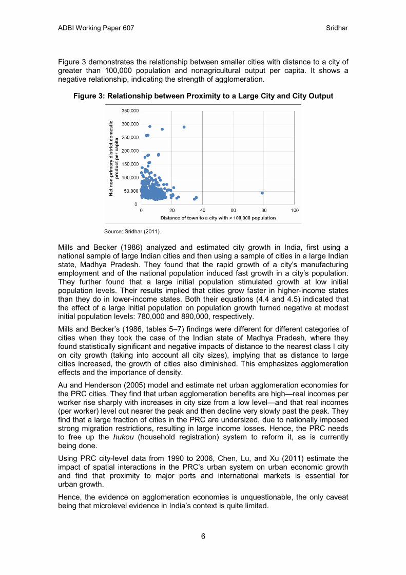
Figure 3 demonstrates the relationship between smaller cities with distance to a city of greater than 100,000 population and nonagricultural output per capita. It shows a negative relationship, indicating the strength of agglomeration.

Figure 3: Relationship between Proximity to a Large City and City Output

Source: Sridhar (2011).

Mills and Becker (1986) analyzed and estimated city growth in India, first using a national sample of large Indian cities and then using a sample of cities in a large Indian state, Madhya Pradesh. They found that the rapid growth of a city’s manufacturing employment and of the national population induced fast growth in a city’s population. They further found that a large initial population stimulated growth at low initial population levels. Their results implied that cities grow faster in higher-income states than they do in lower-income states. Both their equations (4.4 and 4.5) indicated that the effect of a large initial population on population growth turned negative at modest initial population levels: 780,000 and 890,000, respectively. Mills and Becker’s (1986, tables 5–7) findings were different for different categories of cities when they took the case of the Indian state of Madhya Pradesh, where they found statistically significant and negative impacts of distance to the nearest class I city on city growth (taking into account all city sizes), implying that as distance to large cities increased, the growth of cities also diminished. This emphasizes agglomeration effects and the importance of density. Au and Henderson (2005) model and estimate net urban agglomeration economies for the PRC cities. They find that urban agglomeration benefits are high—real incomes per worker rise sharply with increases in city size from a low level—and that real incomes (per worker) level out nearer the peak and then decline very slowly past the peak. They find that a large fraction of cities in the PRC are undersized, due to nationally imposed strong migration restrictions, resulting in large income losses. Hence, the PRC needs to free up the hukou (household registration) system to reform it, as is currently being done. Using PRC city-level data from 1990 to 2006, Chen, Lu, and Xu (2011) estimate the impact of spatial interactions in the PRC’s urban system on urban economic growth and find that proximity to major ports and international markets is essential for urban growth. Hence, the evidence on agglomeration economies is unquestionable, the only caveat being that microlevel evidence in India’s context is quite limited.

6


3. SHARING, MATCHING, AND LEARNING Urban areas improve labor productivity through the mechanisms of sharing, matching, and learning (Puga 2009). Enterprises can reduce production costs through these mechanisms. For consumers, big cities supply more diversified products to meet demand. Furthermore, workers will find it easier to get jobs, accumulate experience, and acquire knowledge. These three mechanisms bring about scale economies in cities, especially for transportation infrastructure facilities, and diversified consumer goods. As the mechanisms of sharing are obvious, recent empirical research focuses on the mechanisms of learning (Puga 2009). Empirical studies have proven the existence of human capital externalities (Rauch 1993). In the US, a 1% increase in the university graduate ratio is shown to boost labor productivity by 0.6%–0.7% (Moretti 2004a) and wage level by 0.6%–1.2% (Moretti 2004b). In India, as in other countries, there is a positive relationship between education and earnings. Figure 4 shows a scatterplot of the relationship between the number of graduates per 1,000 population (greater than 7 years of age) and the average daily earnings of all employees at the state level. This is positive, as we expect and find from other countries. Unfortunately, data on education and earnings are not available for Indian cities.

Figure 4: Relationship between Education and Earnings, Indian States

Note: Data pertain to 2009–2010 for both earnings and education. Source: Datanet India (www.indiastat.com).

The next section summarizes the level, speed, and regional variation with respect to urbanization in the Indian context.

4. URBANIZATION: LEVEL, SPEED, AND REGIONAL VARIATION

India’s urbanization level is low at 31%, according to the 2011 Census, but it is high in absolute terms.3 Over 370 million people live in the cities and towns of India. This is

3 For the Census of India 2011, the definition of urban area is as follows: 1. all places with a municipality, corporation, cantonment board, or notified town area committee; and 2. all other places which satisfied the following criteria:

(i) a minimum population of 5,000, (ii) at least 75% of the male main working population engaged in nonagricultural pursuits, and (iii) a population density of at least 400 persons per square kilometer.

7

http://www.indiastat.com/


more than the population of the US. For the first time, the absolute growth in India’s urban population, 91 million, has been higher than its rural counterpart. The urban growth rate, which had decreased in the last decades, rose in the 2011 Census. India’s urbanization is expected to present not only greater challenges but also higher opportunities due to India’s higher population density (411 persons per square kilometer) compared with that of the PRC (144 persons per square kilometer as of 2011, where the low density of cities is now being criticized4), as per data from the World Bank. 5 The density of the urban population in India was 3,659 persons per square kilometer of land area in 2001. In 2011, this increased to 4,767, if the land area is assumed to be the same.

Table 1: Size Distribution of India’s Cities, 1901–2011 Year Class I Class II Class III Class IV Class V All Citiesa 1901 25 44 144 427 771 1,917 1911 26 38 158 388 750 1,909 1921 29 49 172 395 773 2,047 1931 31 59 218 479 849 2,219 1941 49 88 273 554 979 2,424 1951 76 111 374 675 1,195 3,060 1961 107 139 518 820 848 2,700 1971 151 219 652 988 820 3,126 1981b 226 325 883 1,247 920 3,949 1991c 322 421 1,161 1,451 973 4,615 2001d 414 503 1,391 1,558 1,040 5,161 2011 497 NAa NAa NAa NAa 7,935 NA = not available. Notes: a All cities include cities in class sizes I–VI; columns 2–5 report only class sizes I–V. The Census of India’s definition for various class sizes of cities is as follows: Class I: Population >100,000 Class II: Population of 50,000–99,999 Class III: Population of 20,000–49,999 Class IV: Population of 10,000–19,999 Class V: Population of 5,000–9,999 Class VI: Population <5,000. At the time of writing, the class-wise distribution of cities was not yet published out of the 2011 Census. b In 1981, there was no census held in Assam due to disturbed conditions there. So while during 1901–1971, and 1991–2001, the number of cities reported include those in Assam, in 1981, they exclude Assam. If the reader is interested in comparing the figures on various class size cities for the time period considered without Assam, they are available from the author upon request. c In 1991, there was no census held in Jammu and Kashmir (J&K) owing to disturbed conditions. So while during 1901–1981 and in 2001 the number of cities includes those in J&K, the 1991 list of cities excludes those in J&K. The list of all towns separately for J&K for 1901–1981 and 2001 are available upon request from the author, should there be interest for purposes of comparison. d The 2001 size distribution of cities is provisional, as this was still being finalized by the Census of India at the time this paper was revised. The size distribution of cities for 2001 has been computed by the author based on the list of towns and their populations available from the census at that time. Sources: Sridhar (2007); data for 2011 on the population of cities greater than 100,000 and the total number of all cities are from the Census of India (2011).

4 The low density could be due to the fact that the PRC’s city population includes the agricultural population within its jurisdiction. Another reason for the significant drop in density in recent years is because the PRC cities have expanded fast without creating enough jobs.

5 See http://data.worldbank.org/indicator/EN.POP.DNST

8

http://data.worldbank.org/indicator/EN.POP.DNST


Table 1 describes the size distribution of India’s cities. It shows that there was nearly a 20-fold increase in the number of class I cities in the country during the century.

Before we examine regional variations in urbanization, we study the relationship between national income and urbanization in India over the period 1951–2011. Figures 5 and 6 demonstrate the empirical relationship between total national income (in current prices) and per capita income (in constant, 1993–1994 prices) and urbanization during 1951–2004. The trend lines fitted show a steep positive relationship between the two, being an exponential curve in the case of total national income (Figure 5) and perfectly positive in the case of per capita income (Figure 6).

Figure 5: Relationship between National Income and Urbanization in India, 1951–2011

Source: Planning Commission and Census of India.

Figure 6: Relationship between per Capita Income and Urbanization in India, 1951–2004

Source: Planning Commission and Census of India.

1

11

21

31

41

51

61

71

0 5 10 15 20 25 30 35

Nat

iona

l inc

ome

(in tr

illio

ns o

f Rs)

Urbanization rate

9


What can we forecast about the future of urbanization in India? This paper has argued that Asia’s urbanization will be led by megacities to achieve efficiency, equity, and sustainability. Figure 7 shows the projected number of cities in India by 2015 and it is expected that there will be roughly 41 cities with a population of 1 million–2 million, approximately 13 cities with a population of 2 million–5 million, and 9 cities with a population of 5 million and over, broadly consistent with the rank–size rule. Lusome and Bhagat (2006) report that while there has been a substantial increase in the proportion of rural–urban migrants during 1971–2001, there has also been an increase in the proportion of urban–urban migrants during this period. This paper finds that the share of urban–urban migration of both males and females was comparatively low in the intradistrict stream, but it increased substantially in the interdistrict and interstate streams. As institutions of higher learning, particularly professional and technical institutions, are not available in each district, an urge for higher education motivates urban dwellers as well as some of the rural population to migrate over long distances. This is also partly due to the creation of jobs in the modern sector in major metropolises and big cities (Premi 1990). Based on the above and several other advantages of megacities that have been discussed in this paper, we predict that megacities will continue to be important for India’s urban growth.

Figure 7: India’s Urban Population Projection, 2015

Source: Census of India (2011; www.censusindia.gov.in).

10


5. REGIONAL VARIATION Table 2 describes the regional variation in urbanization across Indian states. The state of Delhi is the most urbanized at 98%, followed by Chandigarh at 97%. The least urbanized is the hilly state of Himachal Pradesh at 10%. It does appear that agglomerations such as Delhi, where there are conurbations of economic activity, sharing of knowledge, and learning on a large scale, are highly urban. Physical barriers such as mountainous and hilly terrain increase the costs of urbanization; hence, states such as Himachal Pradesh are largely rural.

Table 2: Regional Variations in Urbanization in India, 2011 India/State/Union Territory % Urban INDIA 31.16 Himachal Pradesh 10.04 Punjab 37.49 Chandigarh 97.25 Uttarakhand 30.55 Haryana 34.79 National Capital Territory of Delhi 97.50 Rajasthan 24.89 Uttar Pradesh 22.28 Bihar 11.30 Sikkim 24.97 Nagaland 28.97 Manipur 30.21 Mizoram 51.51 Tripura 26.18 Meghalaya 20.08 Assam 14.08 West Bengal 31.89 Jharkhand 24.05 Odishaa 16.68 Chhattisgarh 23.24 Madhya Pradesh 27.63 Gujarat 42.58 Daman and Diu 75.16 Dadra and Nagar Haveli 46.62 Maharashtra 45.23 Andhra Pradesh 33.49 Karnataka 38.57 Goa 62.17 Lakshadweep 78.08 Kerala 47.72 Tamil Nadu 48.45 Puducherry 68.31 Andaman and Nicobar Islands 35.67

a In 2011, the Government of India approved the change in the name of the state of Orissa to Odisha. Source: Census of India (2011; www.censusindia.gov.in).

11


Figure 8 shows that the relationship between urbanization and per capita income for Indian states is positive, as may be seen in the linear trend line fitted to the data. It is interesting to examine that across the world, there is a large number of countries, including those in Africa, which have attained a high level of urbanization at fairly low per capita incomes and low degrees of industrialization. This has been termed the urbanization–industrialization gap, which is observed in the Indian context as well.

Figure 8: Relationship between Per Capita Income and Urbanization, Indian States, 2011

Sources: Census of India and Central Statistical Office.

6. THE URBANIZATION–INDUSTRIALIZATION GAP It is assumed that urbanization and industrialization are highly correlated as observed in the case of the developed countries. In the context of the Indian states, the correlation was computed between the share of industry and services in its net state domestic product (NSDP) and its urbanization for the period 2004–2011. The correlation between urbanization and the share of industry and services was positive, being a high 0.74. Urbanization is only at 31%, on average, for India as a whole, but the share of industry and services in Indian states’ domestic product is 80%. Hence, India’s urbanization is significantly lower than what is suggested by its industrialization, which is largely led by the services sector. This suggests that there is a large urban–rural income gap. Taking into account intermittent periods—2004–2005, 2009–2010, and 2011–2012—for major Indian states, while per capita urban monthly consumption expenditure 6 was Rs1,712, per capita rural expenditure was only Rs1,020, accounting for only 60% of per capita urban expenditure.7 Next we move to a discussion of the determinants of urbanization in the Indian context, taking into account its benefits and costs.

6 We have extensively surveyed the literature, and expenditure has been used to represent income in all cases since reliable income data are not available.

7 This is using the assumption of a uniform recall period (URP), under which consumption expenditure data for all items are collected for a 30-day recall period. Data were available on consumption expenditure using a mixed recall period (MRP), under which consumer expenditure data for five nonfood items (clothing, footwear, durable goods, education, and institutional medical expenses) are collected for a 365-day recall period and the consumption data for the remaining items are collected for a 30-day recall period. There was missing data, however, for Chhattisgarh, Uttarakhand, and Jharkhand for 2004 if MRP were to be used; hence, URP is used.

12


7. BENEFITS AND COSTS OF URBANIZATION: ANALYTICAL FRAMEWORK

This part of the paper is motivated by the theoretical framework provided by Brueckner (1990), which embeds the monocentric city model in an economy experiencing rural–urban migration. When urban and rural real incomes are set equal in the model to guarantee migration equilibrium, an equilibrium city population is determined. This equilibrium city size depends on three key variables: the rural–urban income ratio, the ratio of agricultural rent to urban income, and commuting costs. The analysis in Brueckner (1990) shows that city size varies inversely with the rural–urban income ratio and the commuting cost, and directly with the ratio of agricultural rent to urban income. The intuition for this expectation is clear: First, an increase in the urban income level raises the urban standard of living relative to that in the rural areas, which creates an impetus for migration, as highlighted by the Todaro (1969) model as well, and increases the urban population. Hence, the expected impact of the rural–urban income ratio on urbanization is positive. Similarly, an increase in the commuting cost reduces the real income of the city residents and leads to an equilibrating migration flow to the countryside—hence, the expected impact of commuting cost on urbanization is negative. When agricultural rent rises relative to urban income, real incomes decline for both urban and rural residents. However, since nominal income stays constant in the countryside, while the disposable income of the residents at the urban boundary rises, it follows that real income falls less in the city than in the countryside. The result is migration toward the city, which proceeds until living standards are equalized. Therefore, the expected impact of the ratio of agricultural rent to urban income on urbanization is positive. The model is stated as follows:

U = f (Y,T,R), (1)

where U refers to urbanization, Y is the rural–urban income ratio, T refers to commuting cost, and R is the ratio of agricultural rent to urban income. While equation (1) is written as if the rural–urban income ratio (Y) determines urbanization unilaterally, there could be a two-way, possibly nonlinear, relationship between urbanization and the rural–urban income ratio. We need to clarify this further. In theory, we can have the following two expectations:

1. When we are examining the impact of the rural–urban income ratio (Y) on urbanization, the expected impact is positive—since migrants will perceive the income differential and move to cities. The higher the income differential, the higher the urbanization rate.

2. The rural–urban income ratio (Y) could be endogenous. The expected impact of urbanization on the rural–urban ratio is negative because we expect urbanization to reduce the inequality; a positive impact is possible if urbanization aggravates the rural–urban inequality. Thus, the rural–urban ratio could be endogenous since rural–urban migration, the consequent urbanization, and the demand for and supply of labor could equalize rural–urban incomes and their ratio. If such a thing were to occur, the rural–urban income ratio (Y) is endogenous and would be determined within the model.

13


Both these expectations may or may not be met in reality, but the expectation depends on what our policy variable is. Hence, equation (1) is empirically implemented with data from Indian states by ordinary least squares (OLS) first. In the next step, in order to account for the endogeneity of the rural–urban ratio (Y), an instrumental variables (IV) estimation is performed whereby instruments such as the predicted urbanization from the first-stage OLS and its squared regression (to test for nonlinearity), commuting cost, the ratio of agricultural rent to urban income, and the state’s population are used as exogenous variables and regressed on the rural–urban ratio as the dependent variable. Thus, the predicted value of urbanization from the OLS regression is used as an instrument for its endogeneity in the second step to get unbiased estimates of the impacts of urbanization.

8. DATA AND SOURCES The dataset consists of cross-sectional data for major Indian states on the urbanization rate, urban and rural monthly per capita expenditure (MPCE),8 the ratio of agricultural rent to urban income, and commuting cost (cost per passenger kilometer), for 2004–2005, 2009–2010, and 2011–2012, given these were the only years for which the MPCE data were available from the National Sample Survey Organisation (NSSO). The data on urbanization rates for the Indian states are from the Census of India, 2001 and 2011. Total state population and urbanized population for the states, and for the largest cities in the states, for the intervening years (2004–2005 and 2009–2010) were projected, using an exponential rate assumption. The commuting cost, the cost per passenger kilometer variable, was purchased from the Central Institute of Road Transport, Pune, which publishes these data for the State Road Transport Undertakings (SRTUs). Several states disaggregate this cost per kilometer separately for rural and urban areas. Several states publish data separately for the SRTUs in their biggest cities—such as the Brihanmumbai Electricity Supply and Transport (BEST) Undertaking in Mumbai, Delhi Transport Corporation (DTC), Bangalore Metropolitan Transport Corporation (BMTC), and Ahmedabad Municipal Transport Service (AMTS). The cost per passenger kilometer was derived from the fare structure published by the SRTU. The fare structure on the ordinary city bus services for the first 2 kilometers (km) of the journey was used as the basis for commuting cost per passenger kilometer.9 For instance, if the fare for the first 2 km on the city ordinary buses was Rs4, then the cost per passenger kilometer was deemed to be Rs2. Again, commuting cost in metropolitan areas (such as Bangalore, Delhi, Mumbai, and Ahmedabad) would be higher compared with other urban areas. In states for which data for several SRTUs (e.g., Maharashtra, where there was a state urban fare for ordinary city services and several city SRTUs such as the Thane Municipal Undertaking, Kolhapur Municipal Undertaking, Pune Municipal Undertaking, and the BEST Undertaking) were available, the cost per passenger kilometer was computed as the average for these several undertakings. Further, several states did not have data on fare structure for the years 2004, 2009, and 2011, which were used for the

8 While we attempted to use the ratio of rural–urban incomes in many earlier versions of this paper, there was considerable rural–urban variation across the states, when Indian national accounts data were used by sector, which was not consistent with the evidence from the PRC. Based on an extensive review of the Indian literature on the subject, we decided to use the monthly per capita consumption expenditure for rural and urban areas at the state level, which is much more stable across the Indian states and, possibly for this reason, more extensively used.

9 The metro express and metro deluxe fares were not taken into account.

14


estimation.10 Given this, the average urban fare per passenger kilometer for all India11 was assumed to hold good for these states for the respective years.

9. EMPIRICAL RESULTS The ensuing discussion reports empirical results based on the full sample of 60 observations. First, we report descriptive statistics, followed by scatterplots (Figures 9–16) and the results from the estimations. Table 3 summarizes the basic characteristics of the distribution—mean, median, minimum, and maximum—for the key variables used in the analysis for Indian states for 2004, 2009, and 2011; this is the sample which is used for the estimation.

Table 3: Summary Statistics

Urbanization Rate

Urban–Rural MPCE Ratio

Agricultural Rent–Urban

Income Ratio

Cost per Passenger Kilometer

(Rs)

State Population (in 10,000)

Largest City

Population (in 10,000)

Mean 0.28 1.74 0.25 1.33 5,595.61 280.36

Median 0.28 1.74 0.26 1.38 4,765.04 159.11

Standard Deviation

0.11 0.29 0.10 0.31 4,277.30 298.17

Minimum 0.10 1.16 0.09 0.50 630.12 15.02

Maximum 0.49 2.33 0.50 2.01 19,958.15 1,247.84

MPCE = monthly per capita expenditure. Sources: National Sample Survey Organisation, Central Institute of Road Transport, Census of India, and author’s computations.

In terms of the urban–rural MPCE ratio, the state with the highest ratio of per capita urban–rural expenditure is Chhattisgarh, a state characterized by a significant tribal population. This state, with only 21% urban population in 2004, had one major city—Raipur. The state is characterized by very low rural (Rs425 in 2004) and urban MPCE (Rs990 in 2004) in most NSSO surveys. The poor rural MPCE has been attributed to the decline in per capita food production, poor state of rural infrastructure such as power and roads, and underperformance of social safety net programs like rural job schemes and public distribution systems, which have apparently restricted rural income growth. When we examine the ratio of agricultural rent to urban income, the highest is 0.5 in Punjab, an agriculturally rich state. When we examine commuting cost, the most

10 Data on fare structure for 2004, 2009, and 2011 were missing for several states, including Himachal Pradesh, Punjab, Uttarakhand, Haryana, Uttar Pradesh, Bihar, Assam, Jharkhand, Chhattisgarh, and Madhya Pradesh, among others; for Kerala, the fare structure was missing only for 2004. Based on discussions with the Central Institute of Road Transport from where data were purchased, most of the states for which the fare structure was not published were those which did not offer commuter services in their urban areas—they ran only rural or long-distance services (this was the case with Haryana, Punjab, Bihar, Uttarakhand, and Himachal Pradesh). States such as Jharkhand and Chhattisgarh had no independent public bus services or state transport undertakings at the time the research for this paper was completed. While in Assam, Guwahati city's urban bus service was outsourced to a private operator, that agency had not sent the data on fare structure to the Central Institute of Road Transport. In Uttar Pradesh, the city of Lucknow started offering urban bus services only around 2008–2009.

11 This was determined on the basis of the average fare per passenger kilometer for all the states for which the data were available for the respective years.

15


expensive is Maharashtra, due to the fact that the fare per passenger kilometer in Mumbai and Pune was Rs2.50 even for ordinary services—this includes passenger tax and surcharge, which is not there in most other states. The most urbanized state in the sample is Tamil Nadu at 49% urbanization in 2011. As discussed earlier, Himachal Pradesh is the least urbanized state. While Figures 9–12 show the relationship between urbanization and the urban–rural MPCE ratio, urbanization and the urban commuting cost, urbanization and the ratio of agricultural rent to urban income, and urbanization and the population of the state’s largest city, Figures 13–16 show these relationships between the population of the state’s largest city and the other variables indicated above, respectively. Figure 9 shows that there is a weak negative relationship between urbanization and the urban–rural MPCE ratio, with a negative correlation of –0.04, which is unexpected since a higher urban consumption expenditure (used to indicate income), relative to that of rural areas, would imply that the incentive to migrate and urbanize is minimal and vice versa. However, this relationship is weak and not significant.

Figure 9: Relationship between Urbanization and Urban–Rural Monthly Per Capita Expenditure Ratio

Sources: Census of India, National Sample Survey Organisation various rounds, and author’s computations.

Figure 10 shows a weak positive relationship between urbanization and the urban commuting cost, which is natural to expect, with a positive correlation of 0.02, with the caveats of the data on commuting costs—they are for cities in some cases; in some other cases, they represent an overall urban commuting cost for the state as a whole. As urbanization and city size increase, we expect the commuting cost to also increase commensurately.

Further, Figure 11 shows a negative relationship between urbanization and the agricultural rent–urban income ratio, which is as expected, with a correlation of –0.35.

16


Figure 10: Relationship between Urbanization and Commuting Cost per Kilometer (Rs)

Sources: Census of India, Central Institute of Road Transport, and author’s computations.

Figure 11: Relationship between Urbanization and Ratio of Agricultural Rent–Urban Income

Sources: Census of India, Central Statistical Office, and author’s computations.

Figure 12 shows the relationship between urbanization and state population, demonstrating that there is usually a positive relationship between the two, other things remaining constant. This is reasonable to expect as large states are usually more urban, with the exception of states such as Uttar Pradesh, which is the largest, but has a low urbanization rate. Hence, we may expect large states to be more urban if their income level is also higher. There is a weak positive correlation of 0.11 between the two.

Figure 13 demonstrates the relationship between the urban–rural MPCE ratio and the population of the state’s largest city. In this figure and Figures 15–17, the population of the state’s largest city is taken to be the indicator of urbanization. As we expect, there is a positive relationship between the two (with a positive correlation of 0.35).

17


Figure 12: Relationship between Urbanization and State Population

Sources: Census of India and author’s computations.

Figure 13: Relationship between Urban–Rural Monthly per Capita Expenditure Ratio and Population of the State’s Largest City

Sources: Central Statistical Office, Census of India, and author’s computations.

Figure 14: Relationship between Population of the State’s Largest City and Ratio of Agricultural Rent and Urban Income

Sources: Central Statistical Office, Census of India, and author’s computations.

18


Figure 14 shows the relationship between the state’s largest city and the ratio of agricultural rent to urban income. As in the case of urbanization, this relationship is negative, as expected for reasons discussed earlier, with a negative correlation of –0.31 between the two.

Figure 15 shows the relationship between the population of the state’s largest city and the urban commuting cost. This is positive broadly, as we expect, with a correlation of 0.31, since when cities grow beyond a certain size, the costs outweigh the benefits.

Figure 15: Relationship between Population of the State’s Largest City and Urban Commuting Cost

Sources: Central Institute of Road Transport, Census of India, and author’s computations.

Figure 16 shows the relationship between population of the state’s largest city and state population. There is a positive relationship, as we would expect, with the highest positive correlation (0.50) than among any other variables.

Figure 16: Relationship between Population of the State’s Largest City and State Population (in 10,000)

Sources: Census of India and author’s computations.

0.00

0.50

1.00

1.50

2.00

2.50

0 200 400 600 800 1000 1200 1400

Cost

per

pas

seng

er k

m (i

n Rs

)

Population of the state's largest city (in 10,000)

0

5,000

10,000

15,000

20,000

25,000

0 200 400 600 800 1000 1200 1400

State

Population

Population of the Largest City

19


10. RESULTS FROM REGRESSIONS As discussed earlier, equation (1) was estimated first by ordinary least squares. We report four specifications with two dependent variables and two specifications each—the dependent variables are the urbanization rate of the state and the population of the largest city in the state (Table 4). The exogenous variables are the urban–rural MPCE ratio, the state population, the commuting cost, and the ratio of agricultural rent to income. In one specification, the commuting cost has been excluded since for nearly half of the sample, the cost per passenger kilometer had to be extrapolated using the all-India average, given there were data missing for several states.

Table 4: Urbanization Regressions

Dependent Variable

Urban–Rural MPCE Ratio

Agricultural Rent–Urban

Income Ratio


State Population (in 10,000) R2 F Statistic

Urbanization ratea

–0.07 (–1.61)

–0.52 (–3.71)*** –

0.00 (1.85)* 0.21 4.91

Urbanization rate

–0.07 (–1.62)

–0.53 (–3.73)***

–0.02 (–0.57)

0.00 (1.91)* 0.21 3.72

Population of largest citya

199.12 (1.93)*

–1,176.28 (–3.69)*** –

0.04 (5.66)*** 0.47 16.81

Population of largest city

206.56 (2.06)**

–1,060.58 (–3.38)***

198.15 (2.13)**

0.04 (5.40)*** 0.51 14.54

* statistically significant at the 10% level, ** statistically significant at the 5% level, *** statistically significant at the 1% level, MPCE = monthly per capita expenditure. a Model variant excluding commuting cost. Notes: t-ratios are in parentheses. Intercepts are not reported. All regressions are based on 60 observations. Sources: National Sample Survey Organisation, Central Institute of Road Transport, Census of India, and author’s analyses.

In both the specifications (with and without the commuting cost), the rural–urban ratio has no impact on urbanization. This shows that the rural–urban ratio alone is not adequate to impact the urbanization rate, which is plausible. Urbanization depends on various other enabling conditions, and it would be naïve to assume that the rural–urban ratio impacts urbanization. It is possible that rural residents also do not have perfect information regarding urban incomes to enable them to make a decision to migrate to urban areas. Finally, in the context of India, a large part of the observed urbanization is due to a natural population increase and not due to migration. Hence, the insignificant impact of the rural–urban ratio on urbanization makes perfect sense. Rather, in both the specifications, the ratio of agricultural rent to urban income has a negative and significant impact on urbanization. We would have expected the ratio to impact urbanization positively, because when agricultural rent rises relative to urban income, real incomes decline for both urban and rural residents. However, since nominal income stays constant in the countryside, while the disposable income of the residents at the urban boundary rises, it follows that real income falls less in the city than in the countryside. The result is migration toward the city, which presumably proceeds until living standards are equalized. However, it is probable that if migration does not occur, the sign we have found is plausible. State population has the expected

20


positive impact on urbanization, showing that large states are more likely to be urbanized than their smaller counterparts. When we estimate the population of the largest city in the state, either with or without controlling for commuting costs, the impacts on urbanization are as expected. The rural–urban ratio has the expected positive impact on urbanization, which has a sharper focus, implying that if rural incomes are higher relative to urban incomes (measured by expenditures), migrants would certainly prefer to move to the biggest city in the state. However, the ratio of agricultural rent to urban income has an unexpected negative impact, showing that migration toward the biggest city does not continue until living standards equalize across rural and urban areas in the event of a rise in agricultural rents at the boundary. Hence, this does not translate into a higher population of the largest city in the state. The unexpected finding is the impact of the commuting cost on the size of the largest city, which is positive. This means that higher commuting costs actually lead to a bigger city size, whereas we would have expected a smaller city to have higher commuting costs. This is, in fact, consistent with the literature. Brueckner (1990) reports this strikingly similar but unexpected finding. One reason that we encounter this finding here is the way in which commuting costs are measured. As explained earlier, in some cases (such as Maharashtra, where the cost per passenger kilometer is the average of all the SRTUs in that state), the commuting cost is a representative urban commuting cost for the entire state, whereas in some other states (such as Punjab and Rajasthan), the all-India urban commuting cost per passenger kilometer is used, since the commuting cost specific to various urban areas in these states was not reported. In other cases (including Karnataka and Maharashtra), we had city-specific commuting costs (for Bangalore and Mumbai, respectively). Another caveat of the commuting data is that the cost per kilometer is for all passengers incurred by the SRTU. The fare structure was available for all the SRTUs, but there was not much variation in the cost per passenger kilometer across the states (it was close to Rs1 for most states, consistent with the assumption made by Brueckner and Sridhar [2012]). Another reason could be that the commuting cost is the result of a large city. If we had measured the commuting cost more precisely and uniformly for all states, our results may have been as expected. The total state population has a positive and significant impact on the size of the largest city in the state, implying that it is highly likely for large states such as Uttar Pradesh to have large cities, which is consistent with the corresponding research using cross-national data. The unexpected performance of the ratio of agricultural rent to urban income variable in the urbanization regression suggests that migration does not play an important role in determining the rate of urbanization in India. This is consistent with the insignificant role played by the rural–urban ratio in the urbanization regressions. However, the rural–urban ratio has a positive impact on the largest city’s population, endorsing the idea that while migration does not occur toward urban areas in general, it will likely occur toward the largest city in the state. Further, commuting cost has a positive impact on the largest city population, part of which may be due to the data caveats—in the case of many states, we had to make do with overall state commuting costs, rather than a cost variable applied to urban areas, as explained earlier. As discussed, there could be a two-way relationship between urbanization and the per capita rural–urban ratio. For this, the first-stage OLS regressions were used to predict urbanization rate (or largest city population) for each of the states. The predicted urbanization rate (or largest city population) was used as an exogenous variable along

21


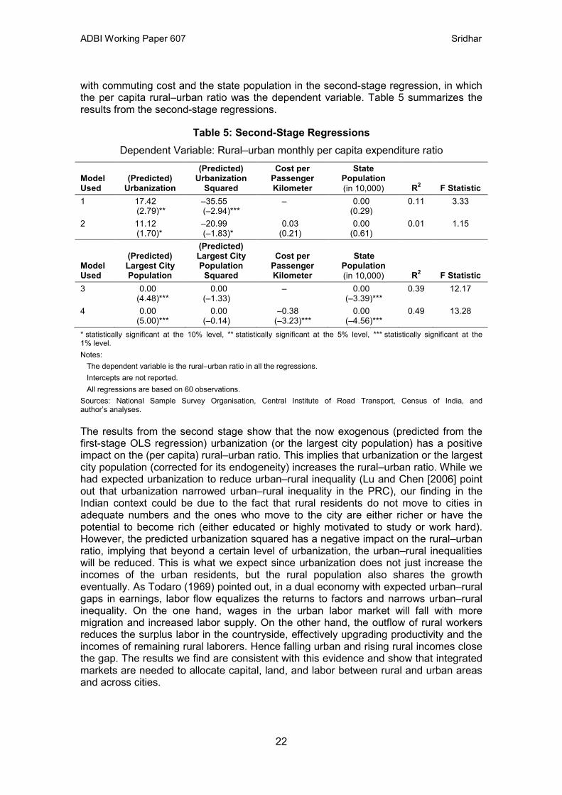
with commuting cost and the state population in the second-stage regression, in which the per capita rural–urban ratio was the dependent variable. Table 5 summarizes the results from the second-stage regressions.

Table 5: Second-Stage Regressions Dependent Variable: Rural–urban monthly per capita expenditure ratio

Model Used

(Predicted) Urbanization

(Predicted) Urbanization

Squared



1 17.42 (2.79)**

–35.55 (–2.94)***

– 0.00 (0.29)

0.11 3.33

2 11.12 (1.70)*

–20.99 (–1.83)*

0.03 (0.21)

0.00 (0.61)

0.01 1.15

Model Used

(Predicted) Largest City Population

(Predicted) Largest City Population

Squared



3 0.00 (4.48)***

0.00 (–1.33)

– 0.00 (–3.39)***

0.39 12.17

4 0.00 (5.00)***

0.00 (–0.14)

–0.38 (–3.23)***

0.00 (–4.56)***

0.49 13.28

* statistically significant at the 10% level, ** statistically significant at the 5% level, *** statistically significant at the 1% level. Notes: The dependent variable is the rural–urban ratio in all the regressions. Intercepts are not reported. All regressions are based on 60 observations. Sources: National Sample Survey Organisation, Central Institute of Road Transport, Census of India, and author’s analyses.

The results from the second stage show that the now exogenous (predicted from the first-stage OLS regression) urbanization (or the largest city population) has a positive impact on the (per capita) rural–urban ratio. This implies that urbanization or the largest city population (corrected for its endogeneity) increases the rural–urban ratio. While we had expected urbanization to reduce urban–rural inequality (Lu and Chen [2006] point out that urbanization narrowed urban–rural inequality in the PRC), our finding in the Indian context could be due to the fact that rural residents do not move to cities in adequate numbers and the ones who move to the city are either richer or have the potential to become rich (either educated or highly motivated to study or work hard). However, the predicted urbanization squared has a negative impact on the rural–urban ratio, implying that beyond a certain level of urbanization, the urban–rural inequalities will be reduced. This is what we expect since urbanization does not just increase the incomes of the urban residents, but the rural population also shares the growth eventually. As Todaro (1969) pointed out, in a dual economy with expected urban–rural gaps in earnings, labor flow equalizes the returns to factors and narrows urban–rural inequality. On the one hand, wages in the urban labor market will fall with more migration and increased labor supply. On the other hand, the outflow of rural workers reduces the surplus labor in the countryside, effectively upgrading productivity and the incomes of remaining rural laborers. Hence falling urban and rising rural incomes close the gap. The results we find are consistent with this evidence and show that integrated markets are needed to allocate capital, land, and labor between rural and urban areas and across cities.

22


The state population has a negative impact on the rural–urban ratio, but it is economically insignificant. If it had been economically significant, it would have implied that large states have plenty of opportunities for reducing urban–rural inequalities. In the specification where the predicted value of the largest city population and its squared value are used, the commuting cost has a negative impact on the rural–urban ratio, implying that lower commuting costs lead to a higher urban–rural inequality and vice versa. Given the significant linkages we find in the regressions between rural and urban areas, and since urbanization cannot be viewed in isolation, the next section focuses on rural employment, taking the case of India’s Mahatma Gandhi National Rural Employment Guarantee Scheme (MGNREGS) and looking at the positive impacts of migrant remittances on rural areas.

11. RURAL EMPLOYMENT AND REMITTANCES Affirming the trend of migration of people from villages to big cities and towns, the Census of India 2011 shows that for the first time, India has added more people in urban centers than in rural areas over a decade. Between 2001 and 2011, the number of people living in urban areas increased from 286 million to 377 million, a rise of 91 million. In comparison, the rural population increased by 90 million, up from 743 million in 2001 to 833 million in 2011.12 Based on the assumption that migration to cities to makes them more congested, and hence is necessarily bad, the Government of India has been trying to counter the trend of rural residents migrating to urban areas in search of jobs, and it has initiated programs to promote rural employment, as discussed in an earlier section. The most important national rural employment scheme is the MGNREGS, a flagship program of the government. Under the MGNREGS, rural households willing to do unskilled manual labor are constitutionally entitled to demand employment up to 100 days a year from their respective gram panchayats.13 The main objectives of the MGNREGS are rural poverty alleviation, prevention of rural–urban migration (similar to the rural subsidy programs in the PRC, sometimes in the name of “new countryside construction”), creation of durable and productive assets, and environmental conservation. Another key aspect of the MGNREGS is the guarantee of 33% reservation of work opportunities for women and equal wages. The works undertaken through the MGNREGS give priority to activities related to water harvesting, groundwater recharge, drought-proofing, and tackling flooding. Its focus on eco-restoration and sustainable livelihoods implies that its success should spur private investment by farmers on their lands. The assumption is that such activities would lead over time to an increase in land productivity, generating a natural demand for labor, which would automatically reduce dependence on the MGNREGS as a source of work. Sridhar and Reddy (2014) answer questions such as whether MGNREGS wages have been above their reservation wages. They estimate the reservation wages as dependent on individual and labor market characteristics, being one of the few studies to do this using Indian data, and compute net benefits from MGNREGS jobs. Next, they investigate what demand-side (individual) and supply-side (program) characteristics determine enrollment in the program and determine MGNREGS wages.

12 See The Indian Express, 16 July 2011. http://archive.indianexpress.com/news/census-data-shows-numbers-rising-more-in-urban-areas/818130/

13 A gram panchayat is the smallest unit of local self-government in India, at the village level.

23


Using data from large primary surveys of MGNREGS beneficiaries and nonbeneficiaries in the Chitradurga District of Karnataka, Sridhar and Reddy (2014) find that the wages MGNREGS beneficiaries received were well below their asking wage (which was Rs207 a day), at an average of only Rs98. Their estimation of reservation wages showed that higher current wages increase reservation wages. The elasticity of reservation wage with respect to work experience was found to be negative, implying that those with higher work experience have lower asking wages, which could be a reflection of the fact that for unskilled rural workers, higher work experience just means older age, which presumably decreases their asking wage. Further, Sridhar and Reddy (2014) estimated a two-step regression model to understand the determinants of participation in the program and of MGNREGS wages. They found that demand-side characteristics, such as age, gender, and the individual’s reservation wages, had a significant impact on enrollment in the program. Supply-side factors, such as per capita program expenditure and percentage of delay in payment of wages, had significant impacts on participation. They concluded that the program has had a favorable impact on reducing poverty. This evidence from India’s (former) MGNREGS, along with the findings from the regressions for urbanization, indicate that rural incomes, when they are high relative to urban incomes, prevent urbanization. The evidence from the MGNREGS seems to indicate that it has impacted poverty by raising rural wages, given that in the case of most of the states, the MGNREGS wages were higher than the minimum wages specified. This prevents migration into cities, which is what the regressions also indicate. Thus, if rural employment programs such as the MGNREGS reduce poverty, these would be adequate to inhibit rural residents from migrating to urban areas. Since its inception in 2006 until 2015, a total of Rs2,690 billion (approximately $44.8 billion) had been spent on the program. Reports of the impact of the program on poverty have been varied. Niehaus and Sukhtankar (2013) found that 89% of workers reported receiving a wage at least as high as their reservation wage in their restricted sample. A study by India’s Institute of Applied Manpower Research (2008), commissioned by the Planning Commission and carried out in 20 districts spread throughout India by targeting 300 beneficiaries from each district, found that one-fourth of the families surveyed were of the opinion that there is migration from their respective village to towns and/or cities in search of jobs. Almost 50% of the households in the western region stated that there is migration from their villages. In the northeastern region, in the district of North Lakhimpur, everyone agreed that there is migration from their villages. There is migration from districts such as South Garo Hills (Meghalaya), Medak (Andhra Pradesh), and Dahod (Maharashtra), in addition to almost all the districts from the eastern region. In some of these districts, the out-migration is as high as 40%. Hence, there is reason to believe that migration to urban areas continues despite the program, and this is consistent with the evidence from Sridhar and Reddy (2014) that their asking wage was well above that offered by the MGNREGS. However, what is it that healthy urbanization entails, which rural development or rural poverty alleviation cannot achieve (see Sridhar 2014)? First, urbanization implies the existence of scale economies, which are possible because of division of labor and specialization. Scale economies explain the existence of factory towns. The existence of large metropolitan areas such as Mumbai, Shanghai, or Chicago is explained by the prevalence of agglomeration economies, the economic efficiencies that arise when firms and people locate in close proximity to one another. Agglomeration economies can be either pecuniary or technological in nature. Pecuniary economies reduce the cost of inputs for firms due to their location in close proximity to each other, while technological economies make inputs more productive.

24


Further, there is a large number of studies that show the impact of density on productivity (Trubka 2007; Carlino, Chatterjee, and Hunt 2007). It may be noted here that all countries, including India, have a density (400 persons per square kilometer in India) or minimum population (5,000 in the Indian context) criterion to define their urban areas. While the data from Indian cities do not permit us to examine the productivity impacts of density conclusively, studies from around the world show that high productivity areas are characterized by high density, whether they are measured by population or employment size and/or employment density. While wages and land rents are higher in metropolitan areas, there should be inherent advantages to firms and residents in locating there; if the costs of locating in metropolitan areas were higher than the benefits, they would not locate in places that would make them worse off. Even when rural–urban migration takes place, there is evidence to show that the rural migrants in urban areas send back remittances to the rural economy. An NSSO report (2010a, cited in Tumbe 2011) estimates that around 58% of the domestic migrants send money home with an average remittance size of Rs13,000 a year.14 This survey found that, on average, during the last 365 days, male out-migrants from urban areas and residing within India had remitted on average nearly Rs28,000.15 Tumbe (2011) confirms this and estimates the domestic remittance market in India to be $10 billion in 2007–2008, with 60% being interstate transfers and 80% being directed toward rural households. Migrant earnings and remittances are used to repay debt; purchase basic necessities; and invest in health, education, and enterprise. The study found that domestic remittances financed over 30% of household consumption expenditure in remittance-receiving households, which formed nearly 10% of rural India (Tumbe 2011).

Figure 17: Per Capita Land Area and Food Grain Production over Time

Sources: Reserve Bank of India’s 2014 Handbook of Statistics on the Indian Economy, Datanet India (www.indiastats.com), Census of India, and author’s computations.

Figure 17 shows the historical movement of per capita availability of cultivable arable land area and per capita production of food grains for rural India. While capturing the historical trend, the graph demonstrates that even while per capita availability of arable

14 See Ken Research at www.news.kenresearch.com/post/78183317098/market-size-of-the-india-domestic-remittance-market

15 See Press Information Bureau at http://pib.nic.in/newsite/erelease.aspx?relid=62559

25

http://www.news.kenresearch.com/post/78183317098/market-size-of-the-india-domestic-remittance-market

http://www.news.kenresearch.com/post/78183317098/market-size-of-the-india-domestic-remittance-market

http://pib.nic.in/newsite/erelease.aspx?relid=62559


and cultivable land declined over the period 1961–2010, per capita production of food grains has remained stable.

Hence, these results are a clear indication that urbanization should not be planned in isolation, but should take into account rural employment and incomes. Urbanization benefits not only the urban area residents and firms through scale economies, agglomeration economies, sharing, matching, and learning, but also rural areas by increasing their incomes through remittances and financing their expenditures.

12. POLICY IMPLICATIONS A majority of the population in Asia is set to be urban, and the sustainability of growth in the countries of the region depends on their urban areas as their engines of growth. While cities in the PRC account for 70% of the nation’s GDP, urban areas in India currently contribute about 65% of GDP (see Sridhar and Wan 2010a, 2010b). Based on several regressions of urbanization, which reflect its benefits and costs in this paper, we find a positive impact of the crucial rural–urban ratio on the population of the largest city in the state, but not on urbanization. This indicates that while the rural–urban ratio is not strong enough to impact urbanization of the state, it impacts the largest city’s population positively, which is plausible. When accounting for the two-way relationship between urbanization and the rural–urban ratio, we find that urbanization (or the largest city’s population) increases the urban–rural inequalities. However, at higher levels, urbanization can be expected to reduce urban–rural inequalities. This is what we expect since urbanization does not just increase incomes of the urban residents, but the rural population also shares the growth, due to the equilibrating labor flows and subsequent equalization of incomes. First, the results suggest that commuting costs are not important in determining the standard of living in urban India, given the data caveats. Nonetheless, there is a strong case to believe that India can and should support the benefits of urbanization and the development of large cities, due to the following reasons: While the supporting data are not available at the city level, there are strong reasons to believe that cities are the engines of economic growth in India, which may be seen by the fact that they contribute to nearly two-thirds of the country’s GDP. Hence, if India is to sustain its macroeconomic growth targets, it is essential to support urbanization. Second, in the case of Indian cities, there is a positive relationship between urbanization and per capita income, and also between national income and urbanization. This is due to the fact that urbanization enables the better matching of labor markets and skills, sharing, and learning, which enable the workforce in urban areas to be more productive compared with their rural counterparts. Third, there is a large rural–urban income gap in India, with rural incomes being significantly lower than urban incomes, which leads to migration toward urban areas in the expectation of equalizing the income differential. Although migration is not the primary source of urbanization in the country, this is confirmed by the regression results. Nonetheless, it should be remembered that providing subsidies to rural areas, or even urban areas for that matter, is problematic. This is because rural employment guarantees or assured income for a limited time period is acceptable, but not sustainable. Rural youth and workers have to find their own employment as market conditions improve in the long run. Similarly, urban areas should grow and contribute to

26


output, income, and productivity based on the strengths of scale economies and agglomeration. In the long run, both market and political economy considerations prevent subsidization of one area at the cost of the other, failing which it may lead to polarization of interest groups and social conflicts. It is tempting to believe that commuting and its costs would slow the growth of cities. Savage and Dasgupta (2006) report that Bangalore’s average travel time (one-way work trip) increased from 24 minutes in 1991 to 40 minutes in 2001–2002. In the United Kingdom, some estimates show that 2.5 hours are added to work-related journeys each week because of congestion. However, there is hope with technology. Given the penetration of the computer, internet, and use of smartphones with 3G and 4G connectivity in the urban areas, it is possible for workers to telecommute, which can possibly obviate the negative impacts of commuting on urban growth.16 Sridhar and Sridhar (2003) find, using data from the Survey of Income and Program Participation (SIPP) of the US, that telecommuting can at best be a complement, not a substitute, for face-to-face interaction. However, the US data for 2000–2010 show that the increase in the number of people telecommuting is larger than the increase in the number of people using transit over the same period. Telecommuting increases employee productivity by reducing the need to travel, by allowing them to work at times when they are likely to be at their best, and by reducing office distractions.17 Panasonic found through its research that 50% of employee time in branch offices was spent on administrative work that was nonproductive. It is therefore looking at the small office home office (SOHO) concept as one of the measures to increase productivity in the future. British Telecom (BT) increased the use of phone conferencing among its staff in the United Kingdom by 30%, where 75% of all phone conferences are replacements for face-to-face meetings. A study by BT that looked at the impact of this decision found that BT reduced carbon dioxide emissions by 54,000 metric tons that year alone, alongside savings of 12 million liters of car fuel, costing an estimated 9.7 million pounds, due to reduction of a staggering 220 million miles of travel and 1,800 years of staff time during the year of study. Telecommuting not only benefits employees but also organizations, by cutting office space costs. IBM has reported savings due to telecommuting of $75 million in real estate expenses related to office space. Contrary to perception, telecommuting could also increase employee participation in organizational activity. BT found that the average conference call involved eight participants, whereas if face-to-face meetings were held, only five traveled on average. According to the Gartner Group, as early as 2002, more than 108 million users worldwide were working outside the boundaries of their enterprise. Evidence of such teleworking has been found in India and Malaysia. Estimates for European countries vary for teleworkers of all types at 4% of the workforce. Estimates of the number of telecommuters in the US vary and range between 3 and 9 million people, roughly 3%–8% of the workforce. Other studies predict for the US that the penetration rate of

16 By definition, telecommuting is the process of commuting to work through communication links rather than through one's physical presence. Telecommuting refers to working at home, nontraditional satellite offices, telecottages, or neighborhood offices. Teleworking refers to the partial or complete substitution of telecommunications technology for the trip to and from the workplace. Ubiquitous broadband connectivity; powerful computers, smartphones, and tablets with productivity- and communication-enhancing applications; sophisticated remote access and monitoring tools; and enterprise-enabled cloud computing have reduced the physical barriers that formerly required employees to be always in their offices.

17 The studies on telecommuting are all part of research in an earlier paper by Sridhar and Sridhar (2003).

27


telecommuting may vary between 5.2% and 10.4% of the workforce compared with the very low levels of about 1.6% projected. A Forrester Research study points out that about 10% of US households maintain a second office at home, bringing about 9 hours of work per week. Summarizing, the important opportunities that would be made possible by telecommuting include cutting real estate costs, increasing employee productivity, reducing carbon emissions, and making our environment cleaner. Telecommuting can also be a productive way of engaging women and other minorities in the labor force since they may not be able to participate in the labor market otherwise. Finally, it should be noted that employee telecommuting implies remote supervision that presents monitoring challenges for the employer, while physical isolation may impede the employee’s involvement in determining valued organizational outcomes. It might also make it difficult for the company to ensure the quality of its services and their delivery time. Thus, it should be noted that telecommuting entails a significant change in management culture, trust on the part of employers, motivation on the part of employees, teamwork, and networking (see Sridhar and Sridhar 2003). Taking the above into account, investments in infrastructure will improve travel time and mobility, which is important to address as cities grow, to keep enlarging the size of the functional labor market (see Bertaud 2014). However, the automatic reaction of policy makers in developing countries is such that they always respond to reducing “congestion” when a city grows, but not necessarily for improving mobility. This should change since improvement in mobility makes a city more productive and enhances its livability (Bertaud 2014; Sridhar 2014). The lesson that India should learn from the PRC’s urbanization is to facilitate greater understanding of Indian cities by enabling data gathering and dissemination about various aspects of urbanization, such as education and income at the city level or, even better, at the individual household level. Currently some of these data are gathered by India’s NSSO and Census town directories, but even as of late 2014, the Census of India’s 2011 town directories had still not been released. The NSSO data unfortunately cannot be aggregated with confidence at the city level, due to the inadequate number of observations represented from cities. If these data are gathered and published in a timely and regular fashion, it will be possible to ascertain the relationship between human capital, density, productivity, and the growth of cities. Research by Au and Henderson (2005) on PRC city sizes and the optimum value of output for a certain size indicated that the PRC’s cities are undersized, leading to huge welfare losses. Hence, the lesson that the PRC should learn from India’s urbanization experience is to gradually remove restrictions on rural–urban migration by reforming the hukou, which is currently being done.

28


REFERENCES Au, C.-C., and J. V. Henderson. 2005. Are Chinese Cities Too Small? Brown University

Working Paper, 5 October. Basu, B., and S. Bandyapadhyay. 2009. Zipf’s Law and Distribution of Population in

Indian Cities. Indian Journal of Physics 83(11): 1575–1582. Bertaud, A. 2014. Cities as Labor Markets. Marron Institute on Cities and the Urban

Environment, Working Paper No. 2. Bertinelli, L., and E. Strobl. 2007. Urbanisation, Urban Concentration and Economic

Development. Urban Studies 44(13): 2499–2510. Brueckner, J. 1990. Analyzing Third World Urbanization: A Model with Empirical

Evidence. Economic Development and Cultural Change 38: 587–610. ———. 2011. Why Cities Exist? Lectures in Urban Economics. Cambridge, MA:

MIT Press. Brueckner, J., and K. S. Sridhar. 2012. Measuring Welfare Gains from Relaxation of

Land-Use Restrictions: The Case of India’s Building-Height Limits. Regional Science and Urban Economics (Special Issue in Honor of Jacques Thisse) 42(6): 1061–1067. DOI: 10.1016/j.regsciurbeco.2012.08.003

Carlino, G. A., S. Chatterjee, and R. M. Hunt. 2007. Urban Density and the Rate of Invention. Journal of Urban Economics 61(3): 389–419.

Castells, D., and V. Royuela. 2011. Agglomeration, Inequality and Economic Growth. Research Institute of Applied Economics Working Paper 2011/14. Barcelona.

Chen, Z., M. Lu, and P. Ni. Forthcoming. Urbanization and Rural Development in the People’s Republic of China. ADBI Working Paper Series. Tokyo: Asian Development Bank Institute.

Chen, Z., M. Lu, and Z. Xu. 2011. Agglomeration Shadow: A Non-Linear Core–Periphery Model of Urban Growth in China (1990–2006). Paper presented at the ADB Workshop on Green Urbanization in Asia, Honolulu, Hawaii, December.

Duranton, G., and D. Puga. 2003. Micro Foundations of Urban Agglomeration Economies. National Bureau of Economic Research (NBER) Working Paper 9931.

Gabaix, X. 1999. Zipf's Law and the Growth of Cities. American Economic Review 89(2): 129–132.

Gilbert, A., and J. Gugler. 1982. Cities, Poverty, and Development: Urbanization in the Third World. New York, NY and Oxford, UK: Oxford University Press.

Henderson, V. J. 2004. Urbanization and Growth. In P. Aghion and S. Durlauf, eds. Handbook of Economic Growth, Volume 1. Amsterdam: North Holland.

Institute of Applied Manpower Research. 2008. All-India Report on Evaluation of NREGA: A Survey of Twenty Districts. New Delhi: Institute of Applied Manpower Research.

Krugman, P. 1995. Urban Concentration: The Role of Increasing Returns and Transport Costs. In Proceedings of the World Bank Annual Conference on Development Economics 1994. Washington, DC: The International Bank for Reconstruction and Development/The World Bank.

29


Lanaspa, L., F. Pueyo, and F. Sanz. 2005. Patrones de urbanización y nivel de desarrollo. Unaaplicaciónempírica. Cuadernos Aragoneses de Economía 15(1): 83–92.

Lu, M., and Z. Chen. 2006. Urbanization, Urban-Biased Policies and Urban–Rural Inequality in China: 1987–2001. Chinese Economy 39(3): 42–63.

Lusome, R., and R. B. Bhagat. 2006. Trends and Patterns of Internal Migration in India, 1971–2001. Paper presented at the Annual Conference of Indian Association for the Study of Population (IASP), Thiruvananthapuram, 7–9 June. https://www.researchgate.net/profile/R_Bhagat/publication/265278165_Trends_and_Patterns_of_Internal_Migration_in_India_1971-2001/links/540a8bb70cf2f2b29a2cd451.pdf

Mathur, O. P. Forthcoming. Regional and Urban Impacts of Foreign Direct Investment in India. ADBI Working Paper Series. Tokyo: Asian Development Bank Institute.

McGee, T. 1971. The Urbanization Process in the Third World: Explorations in Search of a Theory. London, UK: G. Bell and Sons.

Mills, E. S., and C. M. Becker. 1986. Studies in Indian Urban Development. Washington, DC: World Bank and Oxford University Press.

Moretti, E. 2004a. Workers’ Education, Spillovers, and Productivity: Evidence from Plant-Level Production Functions. The American Economic Review 94(3): 656–690.

———. 2004b. Estimating the Social Return to Higher Education: Evidence from Longitudinal and Repeated Cross-Sectional Data. Journal of Econometrics 121(1-2): 175–212.

Niehaus, P., and S. Sukhtankar. 2013. The Marginal Rate of Corruption in Public Programs: Evidence from India. MIT Economics, 16 January. http://economics.mit.edu/files/8711

Paul, S., K. S. Sridhar, A. V. Reddy, and P. Srinath. 2012. The State of Our Cities: Evidence from Karnataka. New Delhi: Oxford University Press.

Premi, M. K. 1990. India. In C. B. Nam, W. J. Serow, and D. F. Sly, eds. International Handbook on Internal Migration. New York, NY: Greenwood Press.

Puga, D. 2009. The Magnitude and Causes of Agglomeration Economies. Paper written for the Journal of Regional Science’s 50th Anniversary Symposium, April. https://ideas.repec.org/a/bla/jregsc/v50y2010i1p203-219.html (retrieved 17 December 2014).

Quigley, J. 2009. Urbanization, Agglomeration and Economic Development. In M. Spence, P. C. Annez, and R. M. Buckley, eds. Urbanization and Growth: Commission on Growth and Development. Washington, DC: World Bank. https://openknowledge.worldbank.org/handle/10986/2582

Rauch, J. E. 1993. Productivity Gains from Geographic Concentration of Human Capital: Evidence from the Cities. Journal of Urban Economics 34(3): 380–400.

Savage, D., and S. Dasgupta. 2006. Governance Framework for Delivery of Urban Services. In 3i Network, ed. India Infrastructure Report 2006: Urban Infrastructure. New Delhi: Oxford University Press.

Sridhar, K. S. 2007. Density Gradients and Their Determinants: Evidence from India. Regional Science and Urban Economics 37(3): 314–344.

30

https://www.researchgate.net/profile/R_Bhagat/publication/265278165_Trends_and_Patterns_of_Internal_Migration_in_India_1971-2001/links/540a8bb70cf2f2b29a2cd451.pdf




———. 2011. Addendum to Determinants of City Growth and Output in India. Review of Urban and Regional Development Studies 23(2–3): 162–165.

———. 2014. How to Make Our Cities More Productive? The Financial Express, 10 September.

Sridhar, K. S., and N. Kashyap. 2014. Benchmarking Cities: Evidence from India. In K. S. Sridhar and G. Wan, eds. Urbanization in Asia: Governance, Infrastructure and the Environment. New Delhi: Springer.

Sridhar, K. S., and A. V. Reddy. 2014. Contribution of the Urban Poor: A Pilot Study from Bengaluru, India. In Inclusive Urban Planning: State of the Urban Poor Report 2013, edited by Ministry of Housing and Urban Poverty Alleviation, Government of India. New Delhi: Oxford University Press.

Sridhar, K. S., and V. Sridhar. 2003. The Effect of Telecommuting on Suburbanization: Empirical Evidence. Journal of Regional Analysis and Policy 33(1): 1–25.

———. 2007. Telecommunications Infrastructure and Economic Growth: Evidence from Developing Countries. Applied Econometrics and International Development 7(2): 37–56.

Sridhar, K. S., and G. Wan. 2010a. Firm Location Choice in Cities: Evidence from China, India, and Brazil. China Economic Review 21(1): 113–122.

———. 2010b. Firm Location Choice in Cities: Evidence from China and India. In A. U. Santos-Paulino and G. Wan, eds. The Rise of China and India: Impacts, Prospects and Implications. Basingstoke, UK: Palgrave Macmillan. pp. 203–219.

Todaro, M. P. 1969. A Model of Labor Migration and Urban Unemployment in Less Developed Countries. American Economic Review 59: 138–148.

Tripathi, S. 2012. Do Large Agglomerations Lead to Economic Growth? Evidence from Urban India. MPRA Paper No. 38227 (posted 20 April).

Trubka, R. 2007. Productivity and the Density of Economic Activity: Preliminary Estimates of Agglomeration Benefits in Australian Cities. Curtin University’s Sustainability Policy Institute. Unpublished paper.

Tumbe, C. 2011. Remittances in India: Facts and Issues. Indian Institute of Management Bangalore, Working Paper 331. Bangalore.

Zhang, K. H. 2002. What Explains China's Rising Urbanisation in the Reform Era? Urban Studies 39(12): 2301–2315.

31

Asian Development Bank Institute paper is organized as follows. First, evidence on urban...

Documents

Transcript of Asian Development Bank Institute paper is organized as follows. First, evidence on urban...