AS and A Level Biology Lesson Element - Cells · Web viewStatistics for Biologists This resource...

Statistics for BiologistsThis resource supports OCR AS and A Level Biology B (Advancing Biology) (H022/H422) and Biology A (H020/H420).

Instructions for teachersIntroductionThe new Biology AS/A Levels require students to develop and use a wider range of mathematical skills, and the change is particularly marked, for those taking AS examinations, in their first year of study, see:

DfE GCE AS and A level subject content for biology, chemistry, physics and psychology, Appendix 6, page 24 - 28:https://www.gov.uk/government/uploads/system/uploads/attachment_data/file/446829/A_level_science_subject_content.pdf

The full list of mathematical skills can also be found in the specification documents for all OCR science AS and A Levels, as well as in the OCR Mathematical Skills Handbooks. The majority of skills are required for both AS and A Level students but the exceptions, required only for A Level, are clearly indicated.

One of the skills to be covered at both AS and A Level is:

M1.9 Select and use a statistical test

This means chi squared, t testing (paired and unpaired) and Spearman’s rank correlation should be covered by all candidates entering for AS Level as well as A level Biology.

As with all the mathematical content of the new qualifications, we are keen that statistics should be done as an integrated part of studying the biology course; therefore, we are encouraging teachers and students to find aspects of the AS course content that lend themselves to statistical analysis.

Here we provide four examples related to AS content from OCR Biology A (H020) and OCR Biology B (H022). We have also provided discussion and answers.

When distributing the questions section to the learners either as a printed copy or as a Word file you can remove the teacher instructions, discussion and answers sections.

Version 1 1 © OCR 2016

https://www.gov.uk/government/uploads/system/uploads/attachment_data/file/446829/A_level_science_subject_content.pdf

https://www.gov.uk/government/uploads/system/uploads/attachment_data/file/446829/A_level_science_subject_content.pdf

Choosing a statistical testStudents often focus on the arithmetic manipulations – plugging numbers into formulae – but the ability to choose the most suitable test and draw appropriate conclusions based on the results is at least as important. The flowchart below is intended as a useful resource to support your teaching of the choice of test. It is helpful for students to see all four ‘on spec’ tests as well as standard deviation laid out in this chart and it should demystify the process of selecting the right test to use.

Please note that this flowchart will not be provided in the assessments.

The necessary formulae will be provided in the assessments so there is no need for students to memorise these.

Flowchart for choosing a statistical test


Statistics for Biologists 1.

Expected ratios of cell types in human bloodRelevant specification contentBiology B 2.1.1 (a) (ii) the preparation of blood smears (films) for use in light microscopy2.1.1 (b) the procedure for differential staining2.1.1 (c) (i) the structure of animal cells as illustrated by a range of blood cells and components as revealed by the light microscope2.1.1 (e) practical investigations using a haemocytometer to determine cell counts3.3.1 (g) the methods used to detect cancers

Biology A2.1.1 (a) the use of microscopy to observe and investigate different types of cell and cell structure in a range of eukaryotic organisms2.1.1 (c) the use of staining in light microscopy 4.1.1 (e) (ii) examination and drawing of cells observed in blood smears

IntroductionLeukaemia is a form of cancer where the bone marrow produces more white blood cells

(leucocytes) than usual. There are several different forms and treatments and outcomes vary

widely. Initial diagnosis is often based on observation of a high white blood cell count in a

blood sample.

In normal human blood red blood cells (erythrocytes, abbreviated to RBC) and white blood

cells (leucocytes, WBC) are present at these concentrations:

RBC: 5 million per microlitre = 5 x 106 µl-1

WBC: 5000 to 10000 per microlitre = 5 x 103 µl-1 to 1.0 x 104 µl-1

To measure concentrations we would need to use a haemocytometer, but in this example

we only have blood smears to observe.

We can still use the information because it allows us to calculate ratios. It will be important

later, when drawing our conclusions, to remember that we are dealing with ratios not

concentrations.


ratio RBC:WBC 1000:1 to 500:1

We're going to focus on the lowest end of this range i.e. we are asking the question:

'Are there so many WBCs, in comparison to RBCs, that this blood sample is outside the normal range?'

Blood SampleA blood sample was taken from a patient and a blood smear was made. A blood smear is

made by spreading a small drop of blood very thinly on a microscope slide. In the thinnest

parts of the smear, it is only one cell thick, allowing individual cells to be observed, identified

by type and counted.

In this case, of the 5092 cells observed, 18 were white bloods cells. That is higher than the

expected number. But is it significantly higher? Is the blood actually abnormal or is this a

result we might quite probably get from blood where the ratio of RBC:WBC is at the low end

of the normal range (500:1)?

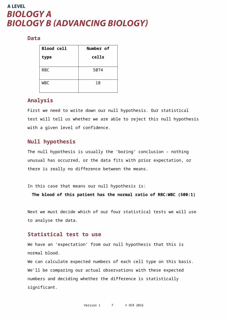
DataBlood cell type Number of cells

RBC 5074

WBC 18

AnalysisFirst we need to write down our null hypothesis. Our statistical test will tell us whether we are

able to reject this null hypothesis with a given level of confidence.

Null hypothesisThe null hypothesis is usually the ‘boring’ conclusion – nothing unusual has occurred, or the

data fits with prior expectation, or there is really no difference between the means.

In this case that means our null hypothesis is:

The blood of this patient has the normal ratio of RBC:WBC (500:1)


Next we must decide which of our four statistical tests we will use to analyse the data.

Statistical test to useWe have an ‘expectation’ from our null hypothesis that this is normal blood.

We can calculate expected numbers of each cell type on this basis.

We’ll be comparing our actual observations with these expected numbers and deciding

whether the difference is statistically significant.

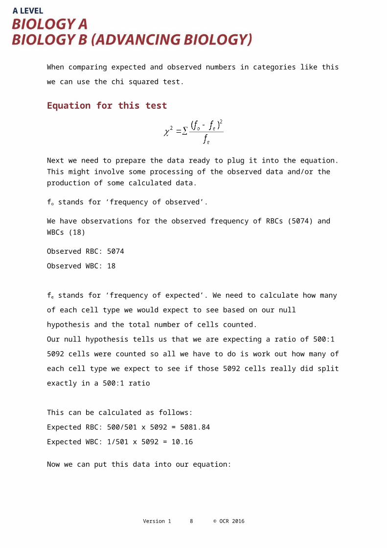
When comparing expected and observed numbers in categories like this we can use the chi

squared test.

Equation for this test

Next we need to prepare the data ready to plug it into the equation. This might involve some processing of the observed data and/or the production of some calculated data.

fo stands for ‘frequency of observed’.

We have observations for the observed frequency of RBCs (5074) and WBCs (18)

Observed RBC: 5074

Observed WBC: 18

fe stands for ‘frequency of expected’. We need to calculate how many of each cell type we

would expect to see based on our null hypothesis and the total number of cells counted.

Our null hypothesis tells us that we are expecting a ratio of 500:1

5092 cells were counted so all we have to do is work out how many of each cell type we

expect to see if those 5092 cells really did split exactly in a 500:1 ratio

This can be calculated as follows:

Expected RBC: 500/501 x 5092 = 5081.84

Expected WBC: 1/501 x 5092 = 10.16

Now we can put this data into our equation:

Remember the Σ symbol in the equation means ‘sum’ so you will add together your calculations of


(observed – expected)2 / expected

for RBCs and WBCs

chi squared = ((5074 - 5081.84)2 / 5081.84) + ((10.16 - 18)2 / 10.16) = 0.0121 + 6.0498 =

6.06

The result is our test statistic.

Test statistic: 6.06

We will compare this with the appropriate critical value from the critical values table for the test we have applied.

To identify the appropriate critical value we need to know the confidence level and the degrees of freedom.

We usually use a confidence level of 95%. This means that the result we have observed would only happen by chance 5% of the time if the null hypothesis is true. So we can be 95% confident in rejecting the null hypothesis if our test statistic really does exceed this critical value.

The degrees of freedom when using the chi squared test is one less than the number of categories. We have two categories in this case so degrees of freedom is one.

The critical value for p=0.05 d.f.=1 can be found in the table at the back of the Mathematical Skills Handbook

Confidence level 95% (p=0.05) Degrees of freedom 1

Critical value: 3.84

Now, by comparing our test statistic with the critical value we can give our conclusion. If the test statistic is greater than the critical value we reject the null hypothesis. We can say, with a certain level of confidence, that the data we observed has not occurred by a chance outcome from a situation where the null hypothesis is true.

Conclusion:Our test statistic exceeds the critical value. Therefore we can reject the null hypothesis. We say that at the 95% confidence level the number of white blood cells found in this sample would not have occurred by chance from a patient with the normal WBC ratio in his/her blood. The WBC ratio in this patient is abnormal.

Notes1. 95% confidence, although it is widely used in A Level biology and many other fields,

is still a relatively weak criterion. Getting a result as apparently-different as this


simply by chance one time in 20 means you might be expecting roughly one student in your class to get such a result (just by chance) in every practical you carry out.For this reason it is also useful, even when you have decided to focus on 95% confidence, to have a look at the adjacent columns - to see how far beyond exceeding the critical value your chi squared result really goes. In this case you can see that if you had decided to hold out for 99% confidence you would have been using a critical value of 6.63. The chi squared value is (slightly) less than this so you would not have rejected the null hypothesis.

2. Should we tell this patient that he/she has leukemia on the basis of our analysis? No. But there are many reasons why not:

We have used ratios not concentrations . All we can say is that the balance between RBCs and WBCs is abnormal. But this could be because this patient has the normal number of WBCs, but unusually low numbers of RBCs. In other words it is just as plausible that the red count is low as that the white count is high.

The confidence level is weak and further tests would definitely be required to confirm / contradict the finding before forming such drastic conclusions.

There are many reasons other than leukemia for a raised white cell count (infection and/or inflammation for example).



Disulfide bonds in thermophilesRelevant specification contentBiology B 2.1.3 (b) the molecular structure of globular proteins as illustrated by the structure of enzymes and haemoglobin2.1.3 (c) how the structure of globular proteins enable enzyme molecules to catalyse specific metabolic reactions2.1.3 (d) (i) the factors affecting the rate of enzyme-catalysed reactions

Biology A2.1.2 (m) the levels of protein structure2.1.2 (n) the structure and function of globular proteins including a conjugated protein2.1.4 (c) the mechanism of enzyme action2.1.4 (d) (i) the effects of pH, temperature, enzyme concentration and substrate concentration on enzyme activity

IntroductionDisulfide bonds can be formed between two cysteine amino acids in a protein, acting to stabilise the folded 3D structure. Until recently, it was thought that disulfide bonds are present almost exclusively in extracellular and compartmentalised proteins, as the reducing environment of the cytoplasm renders disulfide bonds only marginally stable.

However, there is an unusual class of prokaryotes where the intracellular proteins do appear to form disulfide bonds. These prokaryotes are ‘thermophiles’ – thriving in temperatures that would be uninhabitable for most cells.

Could it be that disulfide bonds play a part in stabilising the intracellular proteins of these prokaryotes? If so, we would expect to see increasing numbers of disulfide bonds in the species within this class living at the highest temperatures.

Using genomics databases and information about the ideal growth temperature for each species of thermophile, researchers have compiled data addressing exactly this question.


Species of thermophile Growth temperature (˚C)

Disulfide richness (a.u.)

A. pernix 96 1.22

P. aerophilum 100 1.00

S. solfataricus 81 0.91

Py. horikoshii 95 0.90

Py. furiosus 99 0.85

Py. abysii 97 0.76

S. tokodaii 80 0.75

Thermoplasma volcanium 62 0.68

Thermus thermophiles 76 0.66

Thermococcus kodakaraensis 94 0.65

T. acidophilum 61 0.63

Aquifex aeolicus 86 0.59

Picrophilus torridus 60 0.55

Thermoanaerobacter tengcongensis 75 0.47

Thermotoga maritima 80 0.38

QuestionIs there a significant positive correlation between the number of disulfide bonds in the proteins of a species of thermophile and the temperature at which that species lives?

ReferenceThe data have been adapted from:

Beeby M, O'Connor BD, Ryttersgaard C, Boutz DR, Perry LJ, Yeates TO (2005) The Genomics of Disulfide Bonding and Protein Stabilization in Thermophiles. PLoS Biol 3(9)


Discussion and answersFirst of all we should ensure we understand how the reported data were arrived at. As in the next two examples, the data here have been adapted from the original research paper. I strongly recommend having a look at the original. In particular there is an excellent figure with the data presented as a scattergram.

How did these researchers determine the amount of disulifde bridge bonding in the proteins of thermophiles? It is all based on genomic data. This is interesting and impressive in itself - by using data describing the DNA sequence in a range of thermophiles, by 'decoding' that to give the primary sequence of the resulting proteins, by predicting the 3D fold of those proteins and by identifying instances where two cysteine amino acids are close enough together to make a disulfide bridge the researchers have given each species a 'disulfide bridge score'.

That's pretty cool!

The score is actually on a log scale. However, that doesn't bother us because <spoiler> we'll be assessing correlation using Spearman's rank correlation. That's the only kind of correlation analysis you have to do for OCR Biology AS and A Levels. Because it only looks at the rank order of the data we don't need to worry about what the absolute values of the disulfide score are. If a species is ranked 3rd for disulfide it doesn't matter (in this analysis) whether it is only just below 2nd place or miles above 4th for example.

Confession time. I altered the original data to make it a more useful exercise for AS and A Level. As you'll see if you look at the original paper scattergram, there are several more 'ties' for ideal growth temperature in the original data i.e. there are several cases where two or even three species have the same recorded ideal temperature. This is unfortunate because the Spearman's rank formula you're used to has a 'work around' for ties which becomes increasingly inaccurate the more ties there are. The 'correct' formula for data with many ties is a lot more complicated and I want to keep this as simple as possible while being a) complete enough for AS and A Level purposes and b) interesting (so using real examples instead of made up ones).

So I took the decision to edit out almost all the ties. I left one in so that you can check you know how to deal with it using the 'work around' and the simple formula.

AnalysisWe need a null hypothesis. Let's go with: there is no correlation between ideal growth temperature and disulfide richness in these thermophiles.

(You might have chosen to mention positive correlation in your null hypothesis. That's fine. There are some potentially tricky decisions in statistics tests about using 'one tailed' or 'two tailed' tests. You don't have to wrestle with this complexity at AS and A Level. Exam questions will be phrased so that you're not called upon to decide one- or two-tailed. Once again, then, I'm aiming to keep things as simple as possible while still covering what needs


to be done. We will look for any kind of correlation (negative or positive) and use a two-tailed test.)

We're going to calculate the Spearman's rank correlation coefficient for these data. That will be a number between -1 and +1.

Then, based on how far that coefficient is from 0 and the number of data pairs in our sample, we're going to see whether the positive or negative correlation we've observed is unlikely to have arisen by chance. Specifically we're going to see whether there is a less than 5% (or p=0.05) probability of it arising by chance. If so, we will reject the null hypothesis and call the correlation significant with ‘95% confidence’.

This is how we can develop our results table to give us the numbers we need:


Species of thermophile

Growth temperatur

e (˚C)

Growth Disulfide richness

(a.u.)

Disulfide d Difference in rank

A. pernix 96 4 1.22 1 3 9

P. aerophilum 100 1 1.00 2 1 1

S. solfataricus 81 8 0.91 3 5 25

Py. horikoshii 95 5 0.90 4 1 1

Py. furiosus 99 2 0.85 5 3 9

Py. abysii 97 3 0.76 6 3 9

S. tokodaii 80 9.5 0.75 7 2.5 6.25

Thermoplasma volcanium

6213

0.688 5 25

Thermus thermophiles

7611

0.669 2 4

Thermococcus kodakaraensis

946

0.6510 4 16

T. acidophilum 61 14 0.63 11 3 9

Aquifex aeolicus 86 7 0.59 12 5 25

Picrophilus torridus 60 15 0.55 13 2 4

Thermoanaerobacter tengcongensis

7512

0.4714 2 4

Thermotoga maritima

809.5

0.3815 5.5 30.25

Sum 177.5

Use the Spearman’s rank formula (there’s no need to memorise this – look it up when you need it) and substitute the relevant values n = 15 and Σd2 = 177.5


The Spearman’s rank correlation coefficient rs = 0.6830.

That sounds like a healthy sort of positive correlation. But, given the sample size, does it allow us to reject the null hypothesis? Remember the null hypothesis is that there is no real correlation between disulfide richness and ideal growth temperature. Is there a 5% or more probability that the correlation we have observed in our sample has arisen by chance?

We have a sample size of 15 so we will refer to the n=15 row in the critical values table (in exams you'll be given this, the rest of the time you can use the version in the OCR Biology Mathematical Skills Handbook or many other sources).

We will look first at the 5% (or p=0.05) probability column for a two-tailed test. The value in the table is 0.5214.

If our calculated value is further from zero (remember correlation can be positive or negative) than this critical value we can reject the null hypothesis.

0.6830 is indeed further from zero than 0.5214 so we reject the null hypothesis and say that there is a significant correlation between disulfide richness and ideal growth temperature.

You could stop there but it is always good practice to look at the other columns in the critical values table. In this case you can see that even at 2% and 1% probabilities the critical values are still closer to zero than the coefficient we've calculated (0.6036 and 0.6536 respectively). So we know that the probability that there is in fact no real correlation (and the apparent correlation observed in our sample arose by chance) is less than 0.01 (or 1%).



The effect of IAA on mitotic indexRelevant specification contentBiology B 3.1.1 (a) the cell cycle3.1.1 (b) (i) the changes that take place in the nuclei and cells of animals and plants during mitosis3.1.1 (b) (ii) the microscopic appearance of cells undergoing mitosis

Biology A2.1.6 (c) the main stages of mitosis2.1.6 (d) sections of plant tissue showing the cell cycle and stages of mitosis

IntroductionRoots of Vicia faba (broad bean) were treated with indoleacetic acid (IAA), a plant hormone involved in controlling growth of roots and shoots. All the plants used in the experiment were at the same stage of development. The root treatment lasted 3 hours. At the end of this period the roots were washed to remove the IAA. A number of the roots were immediately fixed, sliced, stained and mounted on microscope slides The other roots were left for a further 5, 11 or 23 hours before fixing, slicing, staining and mounting. Roots from control plants that were not treated with IAA were also fixed, sliced, stained and mounted at the same time intervals as the treated roots to ensure the control in each case was at the same developmental age.

The prepared slides were examined to identify cells in interphase and cells in various stages of mitosis. On each slide 1000 cells were categorised as being in either interphase or mitosis. The mitotic index was then calculated using this formula:

10 slides were examined for each of the 4 treatment groups (0, 5, 11 and 23 h) and each of the matching control groups. The mean mitotic index (and the standard deviation) for each treatment group was calculated.

Fixation (h)

Control

mean mitotic index +/- s.d.

(n = 10)

IAA treatment


(n = 10)

0 6.6 +/- 4.1 5.4 +/- 4.9


5 6.9 +/- 4.3

11 3.8 +/- 2.4 0.5 +/- 0.3

23 5.0 +/- 3.0 0.4 +/- 0.2

QuestionHow long after IAA treatment, if ever, is the rate of mitosis significantly different in treated roots versus untreated controls?


MacLeod, R. D. and Davidson, D. (1966), Changes in Mitotic Indices in Roots of Vicia faba L. New Phytologist, 65: 532–546.

Data from MacLeod and Davidson 1966, Reproduced with permission from John Wiley & Sons.

Discussion and answersAs is often the case with published research, it takes a bit of time and patience when reading the original to work out exactly what protocol has been followed. To add to the complexity, this research was really focused mainly on the effect of another chemical (colchicine) on mitosis. However, the data relating just to IAA were really nice so I used these for this example problem.

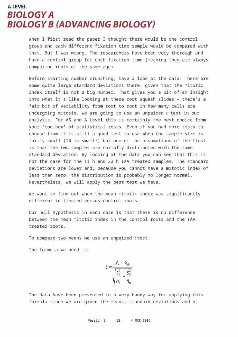
When I first read the paper I thought there would be one control group and each different fixation time sample would be compared with that. But I was wrong. The researchers have been very thorough and have a control group for each fixation time (meaning they are always comparing roots of the same age).

Before starting number crunching, have a look at the data. There are some quite large standard deviations there, given that the mitotic index itself is not a big number. That gives you a bit of an insight into what it's like looking at these root squash slides - there's a fair bit of variability from root to root in how many cells are undergoing mitosis. We are going to use an unpaired t test in our analysis. For AS and A Level this is certainly the best choice from your 'toolbox' of statistical tests. Even if you had more tests to choose from it is still a good test to use when the sample size is fairly small (10 is small!) but one of the assumptions of the t test is that the two samples are normally distributed with the same standard deviation. By looking at the data you can see that this is not the case for the 11 h and 23 h IAA treated samples. The standard deviations are lower and, because you cannot have a mitotic index of less than zero, the distribution is probably no longer normal. Nevertheless, we will apply the best test we have.


We want to find out when the mean mitotic index was significantly different in treated versus control roots.

Our null hypothesis in each case is that there is no difference between the mean mitotic index in the control roots and the IAA treated roots.

To compare two means we use an unpaired t test.

The formula we need is:

The data have been presented in a very handy way for applying this formula since we are given the means, standard deviations and n.

Fixation 0 h

Fixation 5 h

Fixation 11 h

Fixation 23 h

That gives us the t statistic result for each fixation time. Now we will compare each result with the relevant critical value.


Once again we will look first at the column for 5% (p=0.05) level.

The row is chosen according to the number of degrees of freedom. In the case of an unpaired t test this is given by (n1-1)+(n2-1) = (10-1)+(10-1) = 18

The critical value for t at p=0.05 and 18 d.f. is 2.101

Therefore we cannot say that there is a significant difference for fixation 0 h but there is a significant effect for fixations at 5 h and longer.

As always it is good practice to then look at the adjacent columns.

At p=0.02 the critical value is 2.552 and at p=0.01 the critical value is 2.878

Had we been applying the more stringent confidence levels we would not have been able to reject our null hypothesis for fixation 5 h.

The analysis has given us an apparently clear cut answer to the question. From fixation 5 h onwards there is a significant difference in the mitotic index. But it has also given us a more subtle insight: that difference is clearly significant for fixation 11 h and fixation 23 h but it is only deemed significant at the p=0.05 level for fixation 5 h. If fixation 5 h was a crucially important cut off point for some reason, we would be well advised to perform further sampling to confirm or contradict the significance of this apparent effect.



Green tea efficacy in controlling diabetesRelevant specification contentBiology B 2.1.2 (c) (i) how sugar and protein molecules in body fluids can be detected and measured in body fluids and plant extracts5.3.2 (c) the different types of diabetes5.3.2 (d) the fasting blood glucose test, glucose tolerance testing and the use of biosensors in the monitoring of blood glucose concentrations5.3.2 (e) the treatment and management of Type 1 and Type 2 diabetes

Biology A2.1.2 (r) quantitative methods to determine the concentration of a chemical substance in a solution5.1.4 (e) the differences between Type 1 and Type 2 diabetes mellitus5.1.4 (f) the potential treatments for diabetes mellitus

Introduction15 people suffering from Type 2 diabetes took part in a trial to assess the efficacy of green tea in controlling blood glucose concentrations.

Each person was given a ‘glucose tolerance test’ on two successive mornings. They were told not to eat or drink that morning. On the first morning each subject was given a cup of hot water to drink, followed after 10 minutes by a solution containing 75 g glucose. On the second morning each subject drank a cup of green tea, followed after 10 minutes by a solution containing 75 g glucose. On both mornings, blood glucose measurements were taken from each subject 60 minutes after drinking the glucose by using a drop of blood and a biosensor. Once the blood glucose measurement had been taken the subjects were allowed to eat and drink normally for the rest of the day.


Subject Blood glucose concentration following water, day 1 (g dm-3)

Blood glucose concentration following green tea, day 2 (g dm-3)

1 1.6 1.5

2 1.1 1.0

3 1.2 1.0

4 1.7 1.6

5 1.7 1.7

6 1.5 1.3

7 1.6 1.5

8 1.0 1.0

9 1.1 1.0

10 1.3 1.1

11 1.3 1.2

12 1.6 1.4

13 1.0 1.0

14 1.7 1.6

15 1.3 1.2

QuestionDoes green tea have a significant effect on glucose tolerance in Type 2 diabetics?

Reference The data have been adapted from:

Tsuneki H, Ishizuka M, Terasawa M, Wu J-B, Sasaoka T, Kimura I. Effect of green tea on blood glucose levels and serum proteomic patterns in diabetic (db/db) mice and on glucose metabolism in healthy humans. BMC Pharmacology. 2004;4:18


Discussion and answersOnce again, please do have a look at the original research. I have simplified the protocol greatly (in particular the original research follows blood glucose levels over time rather than just taking one measurement) and completely omitted the data from mice. The authors do report a significant effect of green tea but the data I have provided for this statistics example have been altered to make it a useful AS and A Level exercise. So please don’t start drinking green tea on the basis of the conclusions reached here – the effect identified might not be so great in real life.

In particular I have manipulated the data to highlight the purpose of having paired t tests in your statistical toolbox. Many vitally important biological experiments (I’m thinking particularly of trials of the efficacy of medical treatments) are best analysed using a paired t test. By applying the correct test it is sometimes possible to correctly identify significant effects which would have been completely missed if the analysis had used an unpaired t test.

If the quantity being measured varies a lot from person to person, and the effect of the treatment, though genuine, is fairly small it can be very difficult to see the effect if you pool all the data and calculate a mean (which is what the unpaired t test does). It would be theoretically possible to find the effect that way but it might require an impossibly large sample of hundreds of thousands of people.

The clever idea of the paired t test is that rather than pooling all the control data and then pooling all the test data (in many cases where a treatment is being investigated this might be the ‘before’ and ‘after’ data) it is the change in each individual from control to test (or from before to after) that is analysed.

Please note that the pairing of the data can only be done when there is a genuine reason for pairing (most obviously when the two bits of data come from the same individual). What you must never do is pair off the data after collecting it.

This is much easier to understand in the context of the example.

AnalysisWe have data on 15 people with Type 2 diabetes. We can see how each of these people responded to being given a glucose drink on the morning of day 1, following a cup of hot water, and how each of them responded on day 2 when given a glucose drink following a cup of green tea.

Our null hypothesis is that green tea has no effect on glucose tolerance.

This is a perfect opportunity to do a paired t test. The pairing is clear: subject 1 day 1 will be paired with subject 1 day 2 and so on.

(Furthermore the sample is small and the results on day 1 and day 2 have the same standard deviation – it really is ideal for t testing)


This is the data table we need:

Subject

Blood glucose concentration

following water, day 1 (g dm-3)

Blood glucose concentration

following green tea, day 2 (g dm-3)

Difference

d

(g dm-3)

How far is difference from mean difference?

( )

( )2

1 1.6 1.5 0.1 0.007 0.000

2 1.1 1.0 0.1 0.007 0.000

3 1.2 1.0 0.2 0.093 0.009

4 1.7 1.6 0.1 0.007 0.000

5 1.7 1.7 0.0 0.107 0.011

6 1.5 1.3 0.2 0.093 0.009

7 1.6 1.5 0.1 0.007 0.000

8 1.0 1.0 0.0 0.107 0.011

9 1.1 1.0 0.1 0.007 0.000

10 1.3 1.1 0.2 0.093 0.009

11 1.3 1.2 0.1 0.007 0.000

12 1.6 1.4 0.2 0.093 0.009

13 1.0 1.0 0.0 0.107 0.011

14 1.7 1.6 0.1 0.007 0.000

15 1.3 1.2 0.1 0.007 0.000

Total 1.6 0.069

Mean 0.107


Now we need to find the standard deviation of the differences for each individual between day 1 and day 2:

= 0.070

Then we can calculate the t statistic using the formula,

79.8188.1157.39

dsndt = 5.920

The number of degrees of freedom in a paired t test is one less than the number of pairs:

n - 1 = 14

The p value at 5% for 14 degrees of freedom is 2.145. As our value of t is greater than this we can say that the difference is not due to chance and that green tea does have an effect on glucose tolerance in people with Type 2 diabetes.

Once again, looking along the row shows us that even at 2% and 1% probability (98% and 99% confidence levels respectively) we are still able to reject our null hypothesis.

FootnoteThat’s it. However, you might still not be convinced that it is worth knowing about paired t tests as well as unpaired t tests. If we had analysed the same data in an unpaired way, what would we have concluded?

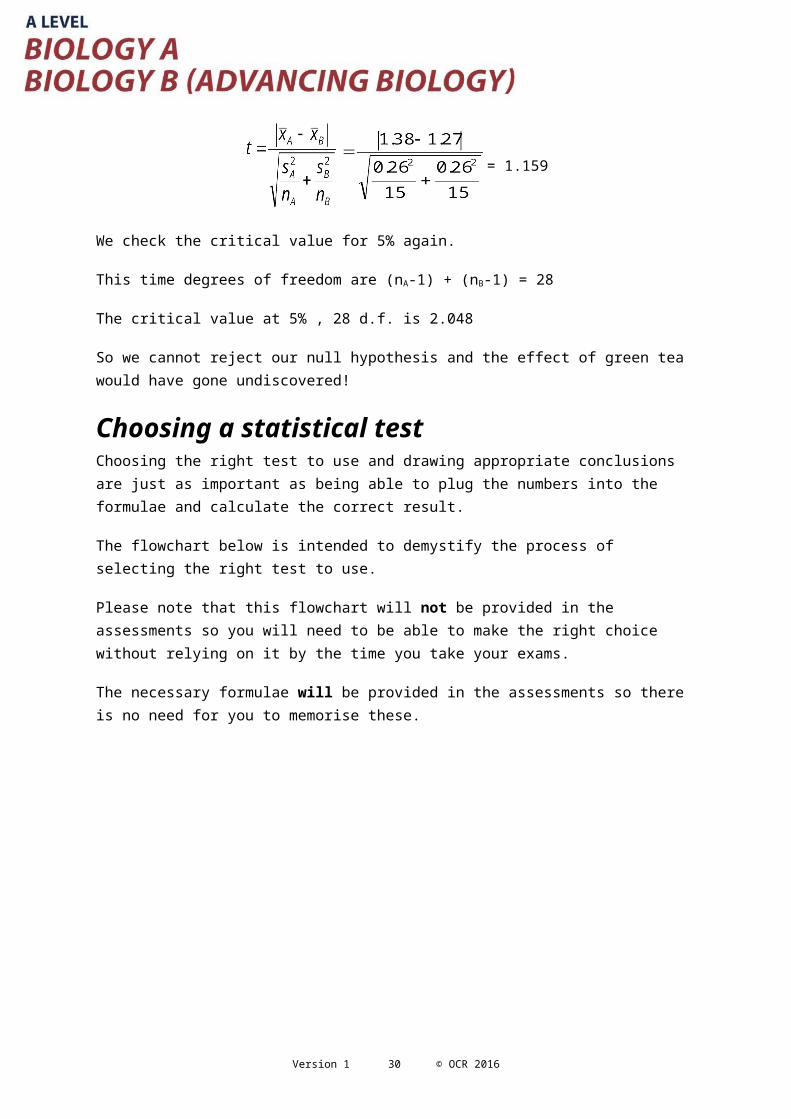
This time we pool all the day 1 measurements to find the mean blood glucose concentration for the controls (it is 1.38 g dm-3). Then we pool all the day 2 measurements to find the mean blood glucose concentration following green tea (it is 1.27 g dm-3). We calculate the standard deviations (both are 0.26) and apply the unpaired formula:

= 1.159

We check the critical value for 5% again.

This time degrees of freedom are (nA-1) + (nB-1) = 28

The critical value at 5% , 28 d.f. is 2.048

So we cannot reject our null hypothesis and the effect of green tea would have gone undiscovered!


Choosing a statistical testChoosing the right test to use and drawing appropriate conclusions are just as important as being able to plug the numbers into the formulae and calculate the correct result.

The flowchart below is intended to demystify the process of selecting the right test to use.

Please note that this flowchart will not be provided in the assessments so you will need to be able to make the right choice without relying on it by the time you take your exams.

The necessary formulae will be provided in the assessments so there is no need for you to memorise these.

Flowchart for choosing a statistical test



Expected ratios of cell types in human bloodRelevant specification contentBiology B 2.1.1 (a) (ii) the preparation of blood smears (films) for use in light microscopy2.1.1 (b) the procedure for differential staining2.1.1 (c) (i) the structure of animal cells as illustrated by a range of blood cells and components as revealed by the light microscope2.1.1 (e) practical investigations using a haemocytometer to determine cell counts3.3.1 (g) the methods used to detect cancers

Biology A2.1.1 (a) the use of microscopy to observe and investigate different types of cell and cell structure in a range of eukaryotic organisms2.1.1 (c) the use of staining in light microscopy 4.1.1 (e) (ii) examination and drawing of cells observed in blood smears

IntroductionLeukaemia is a form of cancer where the bone marrow produces more white blood cells

(leucocytes) than usual. There are several different forms and treatments and outcomes vary

widely. Initial diagnosis is often based on observation of a high white blood cell count in a

blood sample.

In normal human blood red blood cells (erythrocytes, abbreviated to RBC) and white blood

cells (leucocytes, WBC) are present at these concentrations:

RBC: 5 million per microlitre = 5 x 106 µl-1

WBC: 5000 to 10000 per microlitre = 5 x 103 µl-1 to 1.0 x 104 µl-1

To measure concentrations we would need to use a haemocytometer, but in this example

we only have blood smears to observe.

We can still use the information because it allows us to calculate ratios. It will be important

later, when drawing our conclusions, to remember that we are dealing with ratios not

concentrations.

ratio RBC:WBC 1000:1 to 500:1


We're going to focus on the lowest end of this range i.e. we are asking the question:

'Are there so many WBCs, in comparison to RBCs, that this blood sample is outside the normal range?'

Blood SampleA blood sample was taken from a patient and a blood smear was made. A blood smear is

made by spreading a small drop of blood very thinly on a microscope slide. In the thinnest

parts of the smear, it is only one cell thick, allowing individual cells to be observed, identified

by type and counted.

In this case, of the 5092 cells observed, 18 were white bloods cells. That is higher than the

expected number. But is it significantly higher? Is the blood actually abnormal or is this a

result we might quite probably get from blood where the ratio of RBC:WBC is at the low end

of the normal range (500:1)?

DataBlood cell type Number of cells

RBC 5074

WBC 18

AnalysisFirst we need to write down our null hypothesis. Our statistical test will tell us whether we are

able to reject this null hypothesis with a given level of confidence.

Null hypothesis:

Next we must decide which of our four statistical tests we will use to analyse the data.


Statistical test to use:

Equation for this test:

Next we need to prepare the data ready to plug it into the equation. This might involve some processing of the observed data and/or the production of some calculated data.


Now we can put this data into our equation:

The result is our test statistic.

Test statistic:………………………….

We will compare this with the appropriate critical value from the critical values table for the test we have applied.

To identify the appropriate critical value we need to know the confidence level and the degrees of freedom.

Confidence level……………….. Degrees of freedom………………….

Critical value: ………………………..

Now, by comparing our test statistic with the critical value we can give our conclusion. If the test statistic is greater than the critical value we reject the null hypothesis. We can say, with a certain level of confidence, that the data we observed has not occurred by a chance outcome from a situation where the null hypothesis is true.

Conclusion:



Disulfide bonds in thermophilesRelevant specification contentBiology B 2.1.3 (b) the molecular structure of globular proteins as illustrated by the structure of enzymes and haemoglobin2.1.3 (c) how the structure of globular proteins enable enzyme molecules to catalyse specific metabolic reactions2.1.3 (d) (i) the factors affecting the rate of enzyme-catalysed reactions

Biology A2.1.2 (m) the levels of protein structure2.1.2 (n) the structure and function of globular proteins including a conjugated protein2.1.4 (c) the mechanism of enzyme action2.1.4 (d) (i) the effects of pH, temperature, enzyme concentration and substrate concentration on enzyme activity

IntroductionDisulfide bonds can be formed between two cysteine amino acids in a protein, acting to stabilise the folded 3D structure. Until recently, it was thought that disulfide bonds are present almost exclusively in extracellular and compartmentalised proteins, as the reducing environment of the cytoplasm renders disulfide bonds only marginally stable.

However, there is an unusual class of prokaryotes where the intracellular proteins do appear to form disulfide bonds. These prokaryotes are ‘thermophiles’ – thriving in temperatures that would be uninhabitable for most cells.

Could it be that disulfide bonds play a part in stabilising the intracellular proteins of these prokaryotes? If so, we would expect to see increasing numbers of disulfide bonds in the species within this class living at the highest temperatures.

Using genomics databases and information about the ideal growth temperature for each species of thermophile, researchers have compiled data addressing exactly this question.


Species of thermophile Growth temperature (˚C)

Disulfide richness (a.u.)

A. pernix 96 1.22

P. aerophilum 100 1.00

S. solfataricus 81 0.91

Py. horikoshii 95 0.90

Py. furiosus 99 0.85

Py. abysii 97 0.76

S. tokodaii 80 0.75

Thermoplasma volcanium 62 0.68

Thermus thermophiles 76 0.66

Thermococcus kodakaraensis 94 0.65

T. acidophilum 61 0.63

Aquifex aeolicus 86 0.59

Picrophilus torridus 60 0.55

Thermoanaerobacter tengcongensis 75 0.47

Thermotoga maritima 80 0.38

QuestionIs there a significant positive correlation between the number of disulfide bonds in the proteins of a species of thermophile and the temperature at which that species lives?


Beeby M, O'Connor BD, Ryttersgaard C, Boutz DR, Perry LJ, Yeates TO (2005) The Genomics of Disulfide Bonding and Protein Stabilization in Thermophiles. PLoS Biol 3(9)



The effect of IAA on mitotic indexRelevant specification contentBiology B 3.1.1 (a) the cell cycle3.1.1 (b) (i) the changes that take place in the nuclei and cells of animals and plants during mitosis3.1.1 (b) (ii) the microscopic appearance of cells undergoing mitosis

Biology A2.1.6 (c) the main stages of mitosis2.1.6 (d) sections of plant tissue showing the cell cycle and stages of mitosis

IntroductionRoots of Vicia faba (broad bean) were treated with indoleacetic acid (IAA), a plant hormone involved in controlling growth of roots and shoots. All the plants used in the experiment were at the same stage of development. The root treatment lasted 3 hours. At the end of this period the roots were washed to remove the IAA. A number of the roots were immediately fixed, sliced, stained and mounted on microscope slides The other roots were left for a further 5, 11 or 23 hours before fixing, slicing, staining and mounting. Roots from control plants that were not treated with IAA were also fixed, sliced, stained and mounted at the same time intervals as the treated roots to ensure the control in each case was at the same developmental age.

The prepared slides were examined to identify cells in interphase and cells in various stages of mitosis. On each slide 1000 cells were categorised as being in either interphase or mitosis. The mitotic index was then calculated using this formula:

10 slides were examined for each of the 4 treatment groups (0, 5, 11 and 23 h) and each of the matching control groups. The mean mitotic index (and the standard deviation) for each treatment group was calculated.

Fixation (h)

Control


(n = 10)

IAA treatment


(n = 10)

0 6.6 +/- 4.1 5.4 +/- 4.9


5 6.9 +/- 4.3

11 3.8 +/- 2.4 0.5 +/- 0.3

23 5.0 +/- 3.0 0.4 +/- 0.2

QuestionHow long after IAA treatment, if ever, is the rate of mitosis significantly different in treated roots versus untreated controls?


MacLeod, R. D. and Davidson, D. (1966), Changes in Mitotic Indices in Roots of Vicia faba L. New Phytologist, 65: 532–546.

Data from MacLeod and Davidson 1966, Reproduced with permission from John Wiley & Sons.



Green tea efficacy in controlling diabetesRelevant specification contentBiology B 2.1.2 (c) (i) how sugar and protein molecules in body fluids can be detected and measured in body fluids and plant extracts5.3.2 (c) the different types of diabetes5.3.2 (d) the fasting blood glucose test, glucose tolerance testing and the use of biosensors in the monitoring of blood glucose concentrations5.3.2 (e) the treatment and management of Type 1 and Type 2 diabetes

Biology A2.1.2 (r) quantitative methods to determine the concentration of a chemical substance in a solution5.1.4 (e) the differences between Type 1 and Type 2 diabetes mellitus5.1.4 (f) the potential treatments for diabetes mellitus

Introduction15 people suffering from Type 2 diabetes took part in a trial to assess the efficacy of green tea in controlling blood glucose concentrations.

Each person was given a ‘glucose tolerance test’ on two successive mornings. They were told not to eat or drink that morning. On the first morning each subject was given a cup of hot water to drink, followed after 10 minutes by a solution containing 75 g glucose. On the second morning each subject drank a cup of green tea, followed after 10 minutes by a solution containing 75 g glucose. On both mornings, blood glucose measurements were taken from each subject 60 minutes after drinking the glucose by using a drop of blood and a biosensor. Once the blood glucose measurement had been taken the subjects were allowed to eat and drink normally for the rest of the day.


Subject Blood glucose concentration following water, day 1 (g dm-3)

Blood glucose concentration following green tea, day 2 (g dm-3)

1 1.6 1.5

2 1.1 1.0

3 1.2 1.0

4 1.7 1.6

5 1.7 1.7

6 1.5 1.3

7 1.6 1.5

8 1.0 1.0

9 1.1 1.0

10 1.3 1.1

11 1.3 1.2

12 1.6 1.4

13 1.0 1.0

14 1.7 1.6

15 1.3 1.2

QuestionDoes green tea have a significant effect on glucose tolerance in Type 2 diabetics?

Reference The data have been adapted from:

Tsuneki H, Ishizuka M, Terasawa M, Wu J-B, Sasaoka T, Kimura I. Effect of green tea on blood glucose levels and serum proteomic patterns in diabetic (db/db) mice and on glucose metabolism in healthy humans. BMC Pharmacology. 2004;4:18

Copyright © 2004 Tsuneki et al; licensee BioMed Central Ltd.



OCR Resources: the small print

OCR’s resources are provided to support the delivery of OCR qualifications, but in no way constitute an endorsed teaching method that is required by the

Board, and the decision to use them lies with the individual teacher. Whilst every effort is made to ensure the accuracy of the content, OCR cannot be held

responsible for any errors or omissions within these resources.

© OCR 2016 - This resource may be freely copied and distributed, as long as the OCR logo and this message remain intact and OCR is acknowledged as the

originator of this work.

OCR acknowledges the use of the following content: Page 9 & 29 Creative Commons Licence/ Beeby M, O'Connor BD, Ryttersgaard C, Boutz DR, Perry LJ,

Yeates TO (2005) The Genomics of Disulfide Bonding and Protein Stabilization in Thermophiles. PLoS Biol 3(9) Page 14/15 & 30/31 Data from MacLeod and

Davidson 1966, Reproduced with permission from John Wiley & Sons. MacLeod, R. D. and Davidson, D. (1966), Changes in Mitotic Indices in Roots of Vicia faba

L. New Phytologist, 65: 532–546. Page 19 & 33 Creative Commons Licence/Tsuneki H, Ishizuka M, Terasawa M, Wu J-B, Sasaoka T, Kimura I. Effect of green tea

on blood glucose levels and serum proteomic patterns in diabetic (db/db) mice and on glucose metabolism in healthy humans. BMC Pharmacology. 2004;4:18

Copyright © 2004 Tsuneki et al; licensee BioMed Central Ltd.Please get in touch if you want to discuss the accessibility of resources we offer to support delivery of our qualifications: [email protected]

We’d like to know your view on the resources we produce. By clicking on ‘Like’ or ‘Dislike’ you can help us to ensure that our resources work for you. When the email template pops up please add additional comments if you wish and then just click ‘Send’. Thank you.

Whether you already offer OCR qualifications, are new to OCR, or are considering switching from your current provider/awarding organisation, you can request more information by completing the Expression of Interest form which can be found here: www.ocr.org.uk/expression-of-interest

Looking for a resource? There is now a quick and easy search tool to help find free resources for your qualification: www.ocr.org.uk/i-want-to/find-resources/

http://www.ocr.org.uk/i-want-to/find-resources/

http://www.ocr.org.uk/expression-of-interest

mailto:[email protected]?subject=I%20disliked%20A%20Level%20Biology%20A%20and%20Biology%20B%20(Advancing%20Biology)%20Scheme%20of%20Work%20Support

mailto:[email protected]?subject=I%20liked%20A%20Level%20Biology%20A%20and%20Biology%20B%20(Advancing%20Biology)%20Scheme%20of%20Work%20Support

mailto:[email protected]

AS and A Level Biology Lesson Element - Cells · Web viewStatistics for Biologists This resource...

Documents

Transcript of AS and A Level Biology Lesson Element - Cells · Web viewStatistics for Biologists This resource...