arX

iv:h

ep-t

h/93

1217

2v2

27

Dec

199

3

EFI-93-74UCSBTH-93-38hep-th/9312172

On Pair Creation of Extremal Black Holesand Kaluza-Klein Monopoles

Fay Dowker,1a Jerome P. Gauntlett,2 Steven B. Giddings,1b Gary T. Horowitz1c

1Department of Physics

University of California

Santa Barbara, CA 93106aInternet: dowker@cosmic.physics.ucsb.edubInternet: giddings@denali.physics.ucsb.educInternet: gary@cosmic.physics.ucsb.edu

2Enrico Fermi Institute, University of Chicago

5640 S. Ellis Avenue, Chicago, IL 60637

Internet: jerome@yukawa.uchicago.edu

Abstract

Classical solutions describing charged dilaton black holes accelerating in a background

magnetic field have recently been found. They include the Ernst metric of the Einstein-

Maxwell theory as a special case. We study the extremal limit of these solutions in detail,

both at the classical and quantum levels. It is shown that near the event horizon, the

extremal solutions reduce precisely to the static extremal black hole solutions. For a

particular value of the dilaton coupling, these extremal black holes are five dimensional

Kaluza-Klein monopoles. The euclidean sections of these solutions can be interpreted as

instantons describing the pair creation of extremal black holes/Kaluza-Klein monopoles

in a magnetic field. The action of these instantons is calculated and found to agree with

the Schwinger result in the weak field limit. For the euclidean Ernst solution, the action

for the extremal solution differs from that of the previously discussed wormhole instanton

by the Bekenstein-Hawking entropy. However, in many cases quantum corrections become

large in the vicinity of the black hole, and the precise description of the creation process

is unknown.

1. Introduction

The creation of particle-antiparticle pairs in a background field is a common feature of

quantum field theory. Schwinger [1] first studied this process for electrons and positrons in

a uniform electric field. This was extended by Affleck and Manton [2] to the case of GUT

monopole-antimonopole production in a background magnetic field. In general relativity,

the analogue of a monopole is a magnetically charged black hole, and the question naturally

arises as to whether black holes can be pair produced by a background magnetic field. Even

though black holes and monopoles are both “solitons” in the sense of being static extended

objects, there are important differences. First, the configuration of two black holes has

a different spatial topology than the vacuum. So unlike the monopole case, one cannot

continuously deform one into the other. Pair production of black holes is necessarily a

topology changing process. A second difference is simply that the fundamental quantum

theory is known for the case of monopoles (Yang-Mills-Higgs theory) but we still lack a

quantum theory of gravity from which we can calculate black hole pair creation rates from

first principles. Nevertheless, the previous calculations were done in the context of an

instanton approximation, and it seems reasonable to hope that a similar approach will

work for black holes in a sum-over-histories framework for quantum gravity.

Affleck and Manton used an approximate instanton to estimate the pair creation rate

for GUT monopoles. As Gibbons first realized [3], an exact instanton for the Einstein-

Maxwell theory can be obtained by analytically continuing a solution found by Ernst

almost twenty years ago [4]. The Ernst solution describes two oppositely charged black

holes undergoing uniform acceleration in a background magnetic field1. It describes the

evolution of the black holes after their creation. Regularity of the euclidean instanton

turns out to restrict the charge to mass ratio of the black holes. Gibbons believed that

only extremal black holes could be created. But Garfinkle and Strominger [5] found a

regular instanton for which the black holes were slightly non-extremal. Furthermore, the

horizons of the two black holes were identified to form a wormhole in space.

For static charged black holes, the properties of the extremal solution are quite dif-

ferent from the non-extremal one. In particular, the spatial geometry of the extremal

Reissner-Nordstrom metric resembles an infinite throat connected onto an asymptotically

flat region. If extremal black holes of this type can be pair created, one has the intriguing

1 Ernst actually considered electric fields, but by duality, that is equivalent to the magnetic

fields we will consider here.

possibility that an infinite volume of space could be quantum mechanically created in a

finite time. One of the aims of this paper is to investigate this possibility. We explicitly

exhibit an extremal Ernst instanton and study its properties. We will show that as one

approaches the horizon, the solution reduces to the extremal Reissner-Nordstrom solution

with its infinite throat2. Furthermore, we will see that despite the infinite throats, the

action is finite and agrees with Schwinger’s result for weak magnetic fields. (This was also

true for the non-extremal wormhole [5].) However, higher order quantum corrections may

become large down the throat and modify the geometry significantly.

The situation in low energy string theory is similar. Extremal magnetically charged

black holes have a spatial geometry which is identical to that of the Reissner-Nordstrom

solution [7,8]. An effort was made to calculate the production rate for black holes in string

theory [9] by constructing an instanton in a hybrid two- and four-dimensional theory which

was conjectured to approximate the full theory. The resulting configuration described non-

extremal black holes with their horizons identified to form a wormhole. Arguments have

been made that instantons corresponding to the pair creation of extremal black holes do

not exist. We will see that this is incorrect; indeed, in the string case, the natural analogue

of the wormhole instanton develops an infinite throat and becomes extremal. As in the

Reissner-Nordstrom case, this reduces to the static solution far down the throat.

A convenient way to treat both the Einstein-Maxwell and low energy string theories

simultaneously is to consider the action

S =1

16π

∫d4x

√−g[R − 2(∇φ)2 − e−2aφF 2

]. (1.1)

For a = 0 this is the standard Einstein-Maxwell theory coupled to a massless scalar field

φ. By the no-hair theorems, φ must be constant for solutions describing static black holes.

For a = 1, S is part of the action describing the low energy dynamics of string theory. In

this case, φ is not constant outside a charged black hole. For some physical questions it is

more appropriate to use the conformally rescaled metric gµν = e2φgµν which is called the

string metric. It is with respect to this metric that the extremal black holes have infinite

throats. The value a =√3 is also of special interest since this corresponds to standard

2 This can be compared to an instanton found by Brill [6] which describes the splitting of one

throat into many. The present instanton differs in that it includes the asymptotic region and does

not require that a throat be present initially.

Kaluza-Klein theory, i.e. (1.1) is equivalent to the five-dimensional vacuum Einstein action

for geometries with a spacelike symmetry.

The equations of motion which follow from this action are

∇µ(e−2aφFµν) = 0

∇2φ+a

2e−2aφF 2 = 0

Rµν = 2∇µφ∇νφ+ 2e−2aφFµρFνρ − 1

2gµνe−2aφF 2.

(1.2)

Recently a solution to these equations was found (for all values of a) which generalizes the

Ernst solution [10]. These dilaton Ernst solutions describe two oppositely charged black

holes undergoing uniform acceleration in a background magnetic field. They contain a

boost-like symmetry which allows one to analytically continue to obtain euclidean instan-

tons. Regular instantons describing the pair creation of non-extremal black holes with

their horizons identified were constructed in [10] for 0 ≤ a < 1 and shown not to exist for

a ≥ 1. In this paper we will choose the parameters so that the black holes are extremal

and study the resulting instantons for all values of a. As anticipated by Gibbons [3], for

a = 0 the instanton is completely regular. For a = 1, the string metric corresponding to

the extremal instanton is also regular, and for a =√3, the corresponding five dimensional

metric is again regular.

This paper is organized as follows. We begin, in Section 2, by describing the general

features of the lorentzian dilaton Ernst solution and investigate its extremal limit. In this

limit, it is shown that as one approaches the black hole, the solution reduces exactly to

the static black hole solution. Thus for a = 0 and a = 1, the classical extremal accelerated

black holes have infinite throats, just as in the static case. In fact, we will argue that there

is a sense in which the extremal black hole is not accelerating despite the presense of the

magnetic field. However, the region around the black hole is accelerating.

In Section 3 we study the corresponding euclidean instanton. We will show that this

describes creation of a pair of extremal black holes for each value of a. The throats are

not identified to form a wormhole. For fixed values of the physical charge, q, and magnetic

field B, we compute the exact action for both the extremal and wormhole instantons.

For weak fields, i.e. to leading order in qB, the action reduces to the action found by

Schwinger, for all values of a and for both types of instantons. To the next order in qB we

find that, for a = 0, the action of the wormhole instanton is less than that of the extremal

instanton by the Bekenstein-Hawking entropy A/4 of the extremal black holes. We do not

understand the physical significance of this intriguing result which is reminiscent of [11]

in which it was found that the action of the wormhole instanton is less than that of an

instanton describing pair creation of GUT monopoles by the same entropy term. This does

suggest suppression of extremal pair creation relative to that of wormholes, but quantum

corrections can contribute at the same order in qB. For a 6= 0 we find that the actions of

the extremal and wormhole instantons agree even to next order in qB. This is consistent

with the a = 0 result since in this case, the area of the horizon shrinks to zero size in

the extremal limit. (The area of the horizon in the nearly extremal wormhole instanton is

non-zero, but higher order.)

Section 4 contains a discussion of the effect of quantum fluctuations about the clas-

sical solution. This question is of interest in both the lorentzian and euclidean contexts.

Since Hawking’s discovery of black hole evaporation, there has been extensive discussion

of quantum fields around static black holes, and of observers accelerated through the vac-

uum. When the black holes themselves are accelerating, these two subjects are combined

in a fundamental way. By using results from these two areas, we will argue that the back-

reaction may become strong down the infinite throats. For the euclidean instanton, the

quantum fluctuations appear to affect the infinite throats as well, and may substantially

alter the production rate.

The extremal dilaton Ernst solution is of special interest for a =√3, the Kaluza-Klein

case. This is studied in detail in Section 5. It is known that the extremal magnetically

charged black hole for a =√3 is the Sorkin-Gross-Perry monopole [12,13]. So the lorentzian

solution describes two (oppositely charged) monopoles accelerating in a uniform magnetic

field. The euclidean instanton describes pair creation of Kaluza-Klein monopoles. Even

though the four dimensional metric describing an extremal magnetically charged black hole

is singular, the corresponding five dimensional metric turns out to be completely regular.

So the five dimensional instanton is also regular. Unlike the previous cases, the quantum

corrections should remain small everywhere, so the action for the instanton should give a

good approximation to the pair creation rate. We conclude in Section 6 with a discussion

of some open problems.

Before proceeding to the accelerated black hole solutions, we briefly review the static

dilaton black hole and background magnetic field solutions to (1.2). The black hole is

given by [7,8]

ds2 = −λ2dt2 + λ−2dr2 +R2(dθ2 + sin2 θdϕ2)

e−2aφ =(1− r−

r

) 2a2

(1+a2), Aϕ = q(1− cosθ)

λ2 =(1− r+

r

)(1− r−

r

) (1−a2)

(1+a2), R2 = r2

(1− r−

r

) 2a2

(1+a2).

(1.3)

If r+ > r−, the surface r = r+ is the event horizon. For a = 0, the surface r = r− is the

inner Cauchy horizon, however for a > 0 this surface is singular. The parameters r+ and

r− are related to the ADM mass m and total charge q by

m =r+2

+

(1− a2

1 + a2

)r−2, q =

(r+r−1 + a2

) 12

. (1.4)

The extremal limit occurs when r+ = r−. As one approaches this extremal limit, the

Hawking temperature goes to zero when a < 1, approaches a non-zero constant when

a = 1 and diverges when a > 1.

The solution describing the background magnetic field was found by Gibbons and

Maeda [7] and is given by3

ds2 = Λ2

1+a2[−dt2 + dz2 + dρ2

]+ Λ

− 21+a2 ρ2dϕ2

e−2aφ = Λ2a2

1+a2 , Aϕ =Bρ2

2Λ

Λ = 1 +(1 + a2)

4B2ρ2 .

(1.5)

It is a generalization of Melvin’s magnetic universe [14]. The square of the Maxwell field

is F 2 = 2B2/Λ4, which is a maximum on the axis ρ = 0 and decreases to zero at infinity.

The parameter B labels the strength of the magnetic field. For a > 0, the dilaton is zero

on the axis but diverges to minus infinity as ρ→ ∞.

2. Dilaton Ernst metrics

2.1. General properties

The dilaton Ernst solutions to (1.2) constructed in [10] represent two oppositely

charged dilaton black holes uniformly accelerating in a background magnetic field. They

3 The gauge potential given here differs from that in [10] by a gauge transformation so that

Aµ is regular on the axis ρ = 0.

generalize the Einstein-Maxwell (a = 0) solutions found by Ernst [4]. They are:

ds2 = (x− y)−2A−2Λ2

1+a2[F (x)

G(y)dt2 −G−1(y)dy2

+ F (y)G−1(x)dx2

]

+ (x− y)−2A−2Λ− 2

1+a2 F (y)G(x)dϕ2

e−2aφ = e−2aφ0Λ2a2

1+a2F (y)

F (x), Aϕ = − 2eaφ0

(1 + a2)BΛ

[1 +

(1 + a2)

2Bqx

]+ k

(2.1)

where the functions Λ ≡ Λ(x, y), F (ξ) and G(ξ) are given by

Λ =

[1 +

(1 + a2)

2Bqx

]2+

(1 + a2)B2

4A2(x− y)2G(x)F (x)

F (ξ) = (1 + r−Aξ)2a2

(1+a2)

G(ξ) = (1− ξ2 − r+Aξ3)(1 + r−Aξ)

(1−a2)

(1+a2) .

(2.2)

and q is related to r+ and r− by (1.4). The constant k in the expression for the gauge

field is introduced so that the Dirac string of the magnetic field of a monopole is confined

to one axis. The constant φ0 in the solution for the dilaton determines the value of the

dilaton at infinity. Although one could keep this as a free parameter, we will fix it so that

the dilaton vanishes on the axis at infinity in agreement with (1.5). The values of both k

and φ0 will be given below.

The solution (2.1) depends on four other parameters, r±, A, B. Defining m and q via

(1.4) we can loosely think of these parameters together with A,B as denoting the mass,

charge and acceleration of the black holes and the strength of the magnetic field which is

accelerating them, respectively. We emphasize, however, that this is heuristic since, for

example, the mass and acceleration are not in general precisely defined and, further, we

will see that q and B only approximate the physical charge q and magnetic field B in the

limit r±A≪ 1.

It is convenient to introduce the following notation. Define ξ1 ≡ − 1r−A and let ξ2 ≤

ξ3 < ξ4 be the three roots of the cubic in G. The functions F (ξ), G(ξ) then take the form

F (ξ) = (r−A)2a2

1+a2 (ξ − ξ1)2a2

1+a2

G(ξ) = −(r+A)(r−A)(1−a2)

(1+a2) (ξ − ξ2)(ξ − ξ3)(ξ − ξ4)(ξ − ξ1)(1−a2)

(1+a2) .

(2.3)

We restrict the range of the parameters r+ and A so that r+A ≤ 2/(3√3), so that the

ξi are all real; the limit r+A = 2/(3√3) corresponds to ξ2 = ξ3. We also restrict the

parameter r− so that ξ1 ≤ ξ2.

The metric (2.1) has two Killing vectors, ∂∂t and ∂

∂ϕ . The surface y = ξ1 is singular

for a > 0, as can be seen from the square of the field strength. This surface is analogous to

the singular surface (the “would be” inner horizon) of the dilaton black holes. The surface

y = ξ2 is the black hole horizon and the surface y = ξ3 is the acceleration horizon; they

are both Killing horizons for ∂∂t .

The coordinates (x, ϕ) in (2.1) are angular coordinates. To keep the signature of the

metric fixed, the coordinate x is restricted to the range ξ3 ≤ x ≤ ξ4 in which G(x) is

positive. Due to the conformal factor (x − y)−2 in the metric, spatial infinity is reached

by fixing t and letting both y and x approach ξ3. Letting y → x for x 6= ξ3 gives null or

timelike infinity [15]. Since y → x is infinity, the range of the coordinate y is −∞ < y < x

for a = 0, ξ1 < y < x for a > 0.

The norm of the Killing vector ∂∂ϕ

vanishes at x = ξ3 and x = ξ4, which correspond

to the poles of the spheres surrounding the black holes. The axis x = ξ3 points along the

symmetry axis towards spatial infinity. The axis x = ξ4 points towards the other black

hole. The coordinates we are using only cover one region of spacetime containing one of the

black holes. The Dirac string singularities attached to the monopoles will be taken to lie

along the axis x = ξ4; this is accomplished by fixing the constant k so that Aϕ(x = ξ3) = 0.

As discussed in [10], to ensure that the metric is free of conical singularities at both

poles, x = ξ3, ξ4, we must impose the condition

G′(ξ3)Λ(ξ4)2

1+a2 = −G′(ξ4)Λ(ξ3)2

1+a2 . (2.4)

where4 Λ(ξi) ≡ Λ(x = ξi). It will be convenient to define

L ≡ Λ1

1+a2 (ξ3) . (2.5)

When (2.4) is satisfied, the spheres are regular as long as ϕ has period

∆ϕ =4πL2

G′(ξ3). (2.6)

4 It follows from (2.2) that when x is equal to a root of G(x), Λ(x, y) is independent of y. So

Λ(ξi) are constants.

The condition (2.4) can be readily understood in the limit r+A≪ 1, which implies r−A≪1. In this case one has the expansions

ξ2 = − 1

r+A+ r+A+ · · ·

ξ3 = −1− r+A

2+ · · ·

ξ4 = 1− r+A

2+ · · · .

(2.7)

Substituting the expressions (2.2) and (2.3) into (2.4) and expanding to leading order in

r+A gives Newton’s law,

mA ≈ qB , (2.8)

where we have used (1.4) to replace r± with m, q. This is true for all a. More generally, the

condition (2.4) reduces the number of free parameters for the solution to three by relating

the acceleration to the magnetic field, mass, and charge.

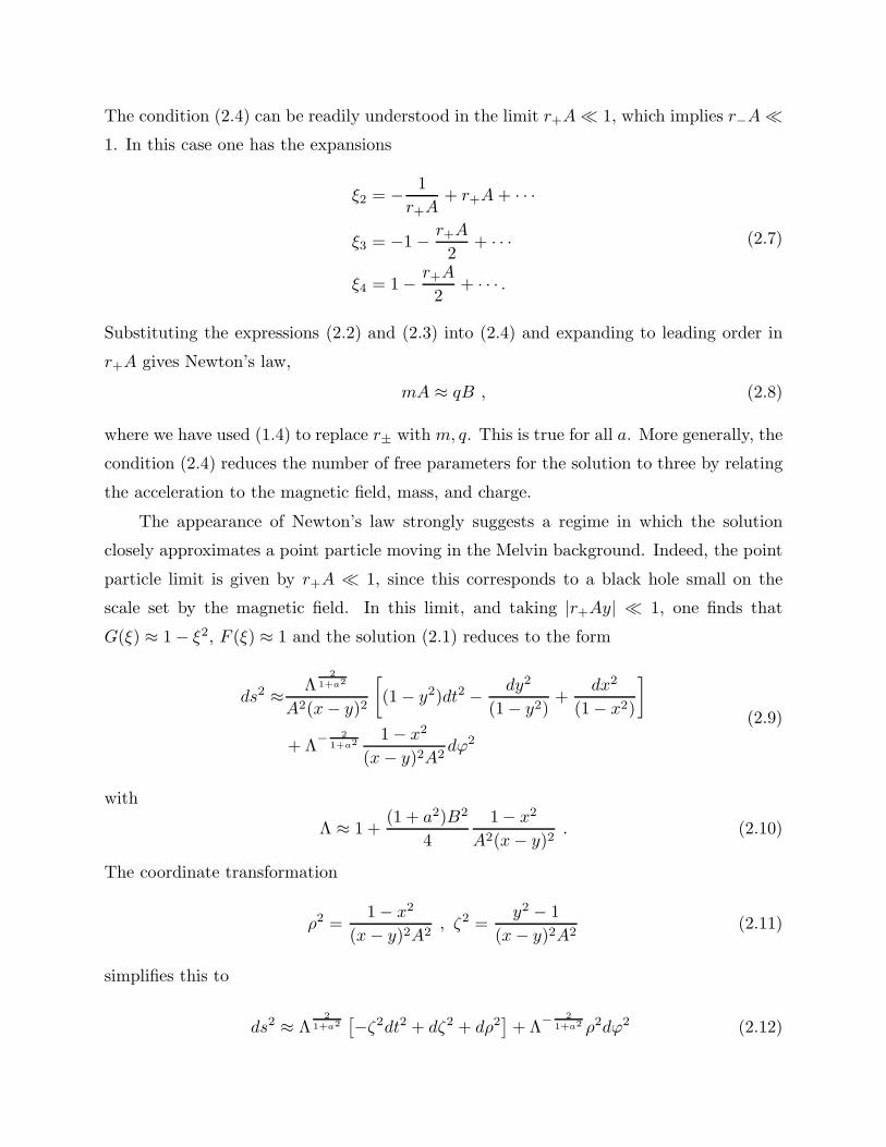
The appearance of Newton’s law strongly suggests a regime in which the solution

closely approximates a point particle moving in the Melvin background. Indeed, the point

particle limit is given by r+A ≪ 1, since this corresponds to a black hole small on the

scale set by the magnetic field. In this limit, and taking |r+Ay| ≪ 1, one finds that

G(ξ) ≈ 1− ξ2, F (ξ) ≈ 1 and the solution (2.1) reduces to the form

ds2 ≈ Λ2

1+a2

A2(x− y)2

[(1− y2)dt2 − dy2

(1− y2)+

dx2

(1− x2)

]

+Λ− 2

1+a21− x2

(x− y)2A2dϕ2

(2.9)

with

Λ ≈ 1 +(1 + a2)B2

4

1− x2

A2(x− y)2. (2.10)

The coordinate transformation

ρ2 =1− x2

(x− y)2A2, ζ2 =

y2 − 1

(x− y)2A2(2.11)

simplifies this to

ds2 ≈ Λ2

1+a2[−ζ2dt2 + dζ2 + dρ2

]+Λ

− 21+a2 ρ2dϕ2 (2.12)

with Λ given in (1.5). The dilaton and gauge fields are likewise found to be

Aϕ ≈ eaφ0Bρ2

2Λ, e−2aφ ≈ e−2aφ0Λ

2a2

1+a2 , (2.13)

where k has been chosen so that A is regular on the axis ρ = 0.

Eqs. (2.12),(2.13) give the dilaton Melvin solution (1.5), expressed in Rindler coordi-

nates, up to the arbitrary shift of the asymptotic value of the dilaton. The standard form

follows using the coordinate transformation t = ζsinht, z = ζcosht. Thus the coordinate

t in the dilaton Ernst solution is the analogue of Rindler time. The subleading terms in

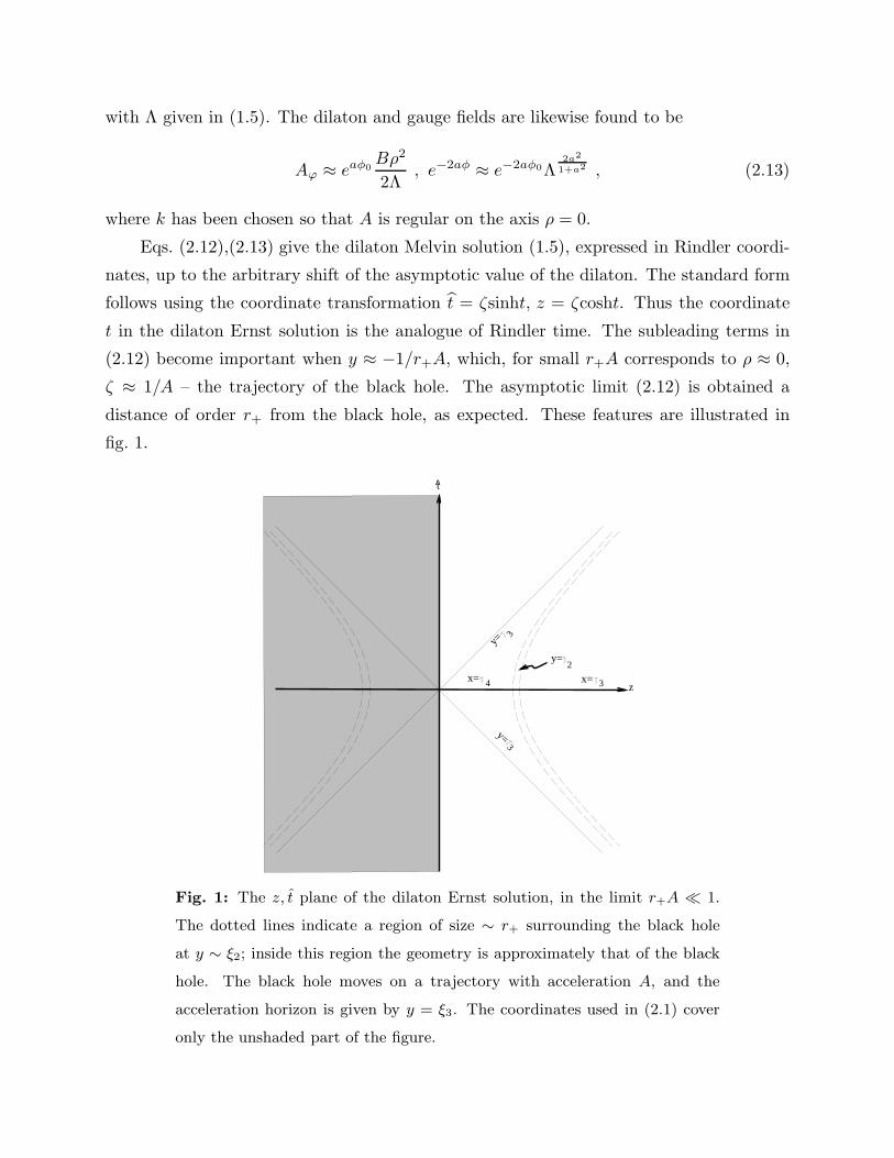
(2.12) become important when y ≈ −1/r+A, which, for small r+A corresponds to ρ ≈ 0,

ζ ≈ 1/A – the trajectory of the black hole. The asymptotic limit (2.12) is obtained a

distance of order r+ from the black hole, as expected. These features are illustrated in

fig. 1.

y=

y=

y=

3

x= x= 34

2

3

z

tv

Fig. 1: The z, t plane of the dilaton Ernst solution, in the limit r+A ≪ 1.

The dotted lines indicate a region of size ∼ r+ surrounding the black hole

at y ∼ ξ2; inside this region the geometry is approximately that of the black

hole. The black hole moves on a trajectory with acceleration A, and the

acceleration horizon is given by y = ξ3. The coordinates used in (2.1) cover

only the unshaded part of the figure.

The relation to Melvin is not restricted to the point-particle limit; even away from

this limit (2.1) becomes Melvin at large spacelike distances. This corresponds to x, y → ξ3.

One way to show that the metric (2.1) approaches (1.5) asymptotically was given in [10].

A somewhat simpler approach is to change coordinates from (x, y, t, ϕ) to (ρ, ζ, η, ϕ) using

x− ξ3 =4F (ξ3)L

2

G′(ξ3)A2

ρ2

(ρ2 + ζ2)2, ξ3 − y =

4F (ξ3)L2

G′(ξ3)A2

ζ2

(ρ2 + ζ2)2

t =2η

G′(ξ3), ϕ =

2L2

G′(ξ3)ϕ

(2.14)

Note that η, ϕ are related to t, ϕ by a simple rescaling and that ϕ has period 2π due to

(2.6). For large ρ2 + ζ2, the dilaton Ernst metric reduces to

ds2 → Λ2

1+a2(−ζ2dη2 + dζ2 + dρ2

)+ Λ

− 21+a2 ρ2dϕ2 (2.15)

where

Λ =

(1 +

1 + a2

4B2ρ2

),

B2 =B2G′(ξ3)

2

4L3+a2 .

(2.16)

Again we recover the dilaton Melvin metric in Rindler coordinates.

The asymptotic form of the dilaton and gauge potential are

e−2aφ → L2a2

Λ2a2

1+a2 e−2aφ0

Aϕ → L−a2

eaφ0Bρ2

2Λ.

(2.17)

This is equivalent to the standard background magnetic field solution (1.5) provided we

choose

eaφ0 = La2

(2.18)

We will take the constant φ0 to be fixed at this value in the remainder of the paper. We

can now see that the physical magnetic field is B given by (2.16). Using (2.7) we note that

in the limit r±A≪ 1, B ≈ B.

The physical charge of the black hole is defined by q = 14π

∫F where the integral is

over any two sphere surrounding the black hole. For the dilaton Ernst solution (2.1), one

obtains

q = qL

3+a2

2 (ξ4 − ξ3)

G′(ξ3)(1 +1+a2

2qBξ4)

. (2.19)

In the weak field limit r±A ≪ 1, q ≈ q. Using (2.16), the product of the physical charge

and magnetic field is

qB =qB(ξ4 − ξ3)

2(1 + 1+a2

2qBξ4)

. (2.20)

This will be useful shortly.

2.2. The limit ξ1 = ξ2: accelerating extremal black holes

Since y = ξ2 is the event horizon and y = ξ1 is an inner horizon (a = 0) or singularity

(a > 0), it follows that the extremal limit of the dilaton Ernst solutions is given by

choosing the parameter r− so that ξ1 = ξ2. Recalling the regularity condition (2.4), it

follows that the extremal solutions are described by two parameters which we can take to

be the physical charge and magnetic field. In this section we will show that as y → ξ2

the extremal solutions become spherically symmetric, and approach the static black hole

solutions (1.3) with r− = r+. This surprising result has a number of consequences which

we will discuss.

Since the derivation involves considerable algebra, we will simply indicate the main

steps involved. The first step is to show that with ξ1 = ξ2, one can divide the condition

for no nodal singularities (2.4) by ξ4 − ξ3 to obtain

1 + (1 + a2)Bqξ2 +1

4(1 + a2)2B2q2(ξ2ξ3 + ξ2ξ4 − ξ3ξ4) = 0 . (2.21)

Taking the limit y → ξ2 and using this equation, the function Λ in (2.1) becomes

Λ → α(x− ξ2) (2.22)

where

α = (1 + a2)Bq +

[(1 + a2)Bq

2

]2(ξ3 + ξ4) . (2.23)

One can then show that the dilaton Ernst metric (2.1) tends to

ds2 → ds20

= −(r+r−)α2

1+a2 (ξ4 − ξ2)(ξ3 − ξ2)(y − ξ2)2

1+a2 dt2

+α

21+a2 r

3a2−1

1+a2

−

A4

1+a2 r+

[dy2

(ξ4 − ξ2)(ξ3 − ξ2)(y − ξ2)2

1+a2

+(y − ξ2)

2a2

1+a2

(x− ξ2)2

(dx2

(x− ξ3)(ξ4 − x)+

4(x− ξ3)(ξ4 − x)

(ξ4 − ξ3)2dϕ2

)]

(2.24)

where we have used the coordinate ϕ introduced in (2.14).

At this stage it is not obvious that the x, ϕ part of the metric (2.24) corresponds to

the round two sphere, but the coordinate change

x =1

2

[ξ3 + ξ4 −

ξ4 − ξ3 + (ξ4 + ξ3 − 2ξ2) cos θ

cos θ + ξ4+ξ3−2ξ2ξ4−ξ3

](2.25)

puts it in the standard form, with polar coordinates θ, ϕ. The final step consists of intro-

ducing a new variable

r2+ =α

2

1+a2 r3a2

−1

1+a2

− (−ξ2)2a2

1+a2

A4

1+a2 r+(ξ4 − ξ2)(ξ3 − ξ2), (2.26)

and new coordinates

t′ =√r+r−(ξ4 − ξ2)(ξ3 − ξ2)(−αξ2)

11+a2 t

y =r+rξ2 .

(2.27)

In the limit y → ξ2, these coordinates simplify (2.24) to

ds20 = −(1− r+

r

) 2

1+a2

dt′2+

(1− r+

r

) −2

1+a2

dr2 + r2+

(1− r+

r

) 2a2

1+a2

dΩ2 . (2.28)

The behavior of the other fields can also be worked out in the limit y → ξ2. One obtains:

Aϕ→ q (1− cosθ) ,

e−2aφ → e−2aφ0 (−αξ2)2a2

1+a2

(1− r+

r

) 2a2

1+a2

,(2.29)

where

q =r+√1 + a2

eaφ0 (−αξ2)−a2

1+a2 (2.30)

This agrees with the extremal static dilaton black hole (given by (1.3) with r+ = r−), in

the limit r → r+.5 Using (2.22) with x = ξ3, ξ4, (2.3) and (1.4) one can show that q agrees

with (2.19) when the black hole is extremal ξ1 = ξ2.

The fact that the extremal dilaton Ernst solution approaches the static black hole as

y → ξ2 has several consequences. First, all the geometric properties of the extremal static

5 Equations (2.28) and (2.29) are exactly the extremal static solution except for a constant

shift in the dilaton.

solutions near the horizon carry over immediately to the accelerated case. In particular,

for a = 0, a constant-t slice of the solution has an infinitely long throat. For a = 1, the

string metric ds2 = e2φds2 also has an infinite throat in which the solution takes the form

of the linear dilaton vacuum. For a =√3, the four-metric, dilaton and gauge field together

make up the five dimensional metric of the Kaluza-Klein monopole (see Section 5).

A second consequence is that there is a sense in which the extremal black holes are

not accelerating. For a = 0, this is suggested by the fact that the event horizon is exactly

spherical. But a more convincing argument comes from examining the acceleration of a

family of observers near the horizon whose four velocities are proportional to ∂/∂t. For

the static black hole, the acceleration of these observers approaches the finite limit 1/q as

they approach the horizon. (This is related to the fact that the surface gravity vanishes for

extremal black holes and is in contrast to the non-extremal case in which the acceleration

diverges.) If one computes the acceleration of these observers for the Ernst solution, one

again finds that it approaches 1/q as y → ξ2 independent of direction. Although this

particular argument cannot be extended to a > 0 since the acceleration (in the Einstein

metric) now diverges for the static extremal solution near the horizon, other arguments

can be made. For example, when a = 1, in the string metric the acceleration of these

observers tends to zero down the throat. In addition, when a =√3, y = ξ2 is a regular

origin in the five dimensional Kaluza-Klein solution, and one can show that its worldline

is a geodesic!

Even though the black hole itself is not accelerating, the region around the black hole

is. This is clear from the relation between the solution and the dilaton Melvin solution

in accelerating coordinates discussed in the previous subsection. In terms of the infinite

throats, one might say that the mouth of the throat is accelerating while the region down

the throat is not.

A final comment concerns the physical charge and magnetic field. Consider the prod-

uct qB. This is small in the weak field limit, which corresponds to ξ2 being large and

negative. What happens when, instead, ξ2 approaches ξ3? The two roots ξ2 and ξ3 can

approach each other only if ξ2, ξ3 → −√3 and ξ4 →

√3/2. Using this, eq. (2.20), and the

no strut condition (2.21), one can show

qB → 1

1 + a2. (2.31)

Thus there is an upper bound on the product of the charge and magnetic field. Roughly

speaking, since the size of an extremal black hole is ∼ q and the width of the Melvin

flux tube is ∼ 1/(B√1 + a2), one of the consequences of (2.31) is that the black holes

are moving in flux tubes wider than themselves. The limit ξ2 → ξ3 corresponds to the

event horizon approaching the acceleration horizon. Since we have assumed the black holes

are extremal, ξ1 = ξ2, this corresponds to a “triple point” where three roots coincide. If

one relaxes the condition ξ1 = ξ2 it appears that the bound on qB is even lower, which

is consistent with the fact that the event horizon is larger than the charge and hits the

acceleration horizon at a smaller value of q. What happens if one takes a charged black

hole and turns up the magnetic field larger than the bound (2.31)? It would appear that

this situation is no longer described by the class of solutions (2.1). The question of what

happens physically is currently under investigation.

3. Dilaton Ernst Instantons

Euclideanizing (2.1) by setting τ = it, we find that another condition must be imposed

on the parameters in order to obtain a regular solution. Two distinct ways that this may be

achieved were discussed in [10] and are reviewed in the first subsection below. These include

the wormhole instantons. There is a third way which leads to the extremal instantons and

is described in the second subsection. The calculation of the action for the wormhole and

extremal instantons is given in the third subsection.

3.1. Wormhole Instantons

In the lorentzian solutions, the vector ∂/∂t is timelike only for ξ2 < y < ξ3. In [10] the

restriction ξ1 < ξ2 was made so that the Einstein metric had a regular horizon for a > 0.

In this case, one must impose a condition on the parameters in order to eliminate conical

singularities in the euclidean solution at both the black hole (y = ξ2) and acceleration

(y = ξ3) horizons with a single choice of the period of τ . This is equivalent to demanding

that the Hawking temperature of the black hole horizon equal the Unruh temperature of

the acceleration horizon.

In terms of the metric function G(y) appearing in (2.1), the period of τ is taken to be

∆τ =4π

G′(ξ3)(3.1)

and the constraint is

G′(ξ2) = −G′(ξ3), (3.2)

yielding

(ξ2 − ξ1ξ3 − ξ1

) 1−a2

1+a2

(ξ4 − ξ2)(ξ3 − ξ2) = (ξ4 − ξ3)(ξ3 − ξ2). (3.3)

With ξ1 < ξ2 there are two ways to satisfy this condition and correspondingly two types

of instantons. The first one exists when ξ2 6= ξ3 and only for 0 ≤ a < 1. It has topology

S2×S2−pt and is interpreted as describing the creation of two oppositely charged dilaton

black holes joined by a wormhole. These “wormhole” instantons generalize the Einstein-

Maxwell instanton discussed in [5]. The reason these instantons only exist for 0 ≤ a < 1

can be understood by recalling the thermodynamic behavior of the dilaton black holes as

extremality is approached: the Hawking temperature, as defined from the period of τ in

the euclidean section, goes to zero for 0 ≤ a < 1, approaches a constant for a = 1 and

diverges for a > 1. Thus, for small magnetic fields and hence accelerations, we expect to

be able to match the resultant Unruh temperature and the black hole temperature by a

small perturbation of the black hole away from extremality only for 0 ≤ a < 1.

The second class of instantons we mention only for completeness since their interpre-

tation is obscure. They are defined by ξ2 = ξ3 which is equivalent to r+A = 2/(3√3), and

have topology S2 ×R2. They are related to the upper limit on qB given by (2.31). Note

that for these instantons one does not have to impose the condition (2.4) for regularity.

3.2. Extremal Instantons

The wormhole type instantons discussed above were made regular by the condition

that the temperatures of the black hole and acceleration horizons should be equal. Gibbons

[3] pointed out (for a = 0) that there is another way that the temperatures of the black

hole and acceleration horizons can be equal: that is if the black hole is extremal. This

might seem strange since extremal dilaton black holes have zero temperature in the sense

that the euclidean time coordinate need not be periodically identified to obtain a regular

geometry. But, of course we can periodically identify the euclidean time and with any

period we like (just as for flat space). In particular we can choose the period forced on us

by having to eliminate a conical singularity elsewhere in the spacetime.

τ

y

event horizon

accelerationhorizon

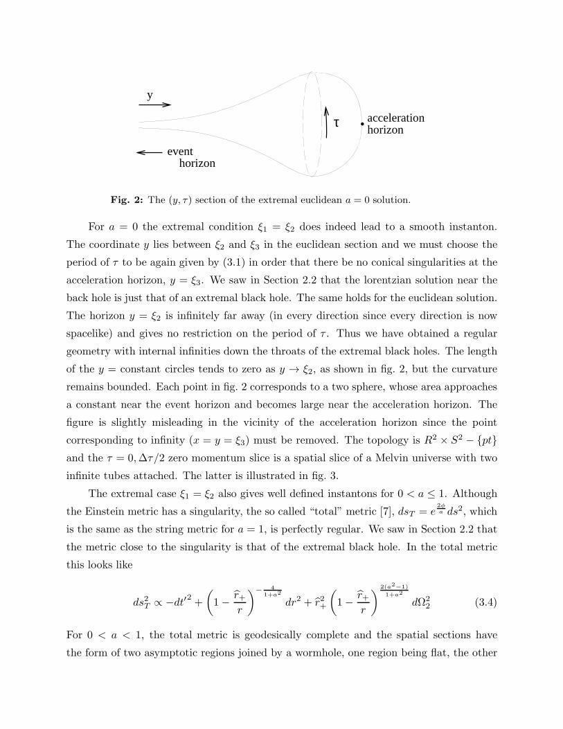
Fig. 2: The (y, τ) section of the extremal euclidean a = 0 solution.

For a = 0 the extremal condition ξ1 = ξ2 does indeed lead to a smooth instanton.

The coordinate y lies between ξ2 and ξ3 in the euclidean section and we must choose the

period of τ to be again given by (3.1) in order that there be no conical singularities at the

acceleration horizon, y = ξ3. We saw in Section 2.2 that the lorentzian solution near the

back hole is just that of an extremal black hole. The same holds for the euclidean solution.

The horizon y = ξ2 is infinitely far away (in every direction since every direction is now

spacelike) and gives no restriction on the period of τ . Thus we have obtained a regular

geometry with internal infinities down the throats of the extremal black holes. The length

of the y = constant circles tends to zero as y → ξ2, as shown in fig. 2, but the curvature

remains bounded. Each point in fig. 2 corresponds to a two sphere, whose area approaches

a constant near the event horizon and becomes large near the acceleration horizon. The

figure is slightly misleading in the vicinity of the acceleration horizon since the point

corresponding to infinity (x = y = ξ3) must be removed. The topology is R2 × S2 − ptand the τ = 0,∆τ/2 zero momentum slice is a spatial slice of a Melvin universe with two

infinite tubes attached. The latter is illustrated in fig. 3.

The extremal case ξ1 = ξ2 also gives well defined instantons for 0 < a ≤ 1. Although

the Einstein metric has a singularity, the so called “total” metric [7], dsT = e2φa ds2, which

is the same as the string metric for a = 1, is perfectly regular. We saw in Section 2.2 that

the metric close to the singularity is that of the extremal black hole. In the total metric

this looks like

ds2T ∝ −dt′2 +(1− r+

r

)− 41+a2

dr2 + r2+

(1− r+

r

) 2(a2−1)

1+a2

dΩ22 (3.4)

For 0 < a < 1, the total metric is geodesically complete and the spatial sections have

the form of two asymptotic regions joined by a wormhole, one region being flat, the other

Fig. 3: The spatial slice τ = 0,∆τ/2 through the instanton solution of fig. 2.

The geometry corresponds to an asymptotically Melvin region, with two ex-

tremal throats attached. The solution may be continued to lorentzian signa-

ture along this slice.

having a deficit solid angle. Hence the corresponding extremal instantons are regular. For

a = 1 the geometry of the string metric is that of an infinitely long throat of constant radius

and thus the a = 1 extremal instanton looks very much like that of the a = 0 extremal

instanton described above (see fig. 4): the topology is the same, R2 × S2 − pt, and the

major difference is that the proper radius of y =constant circles in the (y, τ) section tends

to a finite limit as y → ξ2. The τ = 0, ∆τ2

slice resembles the one shown in figure 3.

τ

y

event horizon

accelerationhorizon

Fig. 4: The (y, τ) section of the euclidean a = 1 solution in the string metric.

For a > 1, both the Einstein metric and the total metric have a naked singularity in

the extremal limit. It has been argued in [16], however, that these “black holes” should be

interpreted as elementary particles. The extremal instantons can then be interpreted as

pair creating such objects. For a =√3 the instanton can also be understood as describing

the creation of a Kaluza-Klein monopole-anti-monopole pair (see Section 5).

Finally we discuss how these different classes of instantons fit together in parameter

space. The parameters of both the extremal and the wormhole type instantons are re-

stricted by the no-nodal singularities condition (2.4). The wormhole instantons are further

restricted by (3.3) and this condition is plotted in fig. 5 for various values of a. The ex-

tremal instantons satisfy ξ1 = ξ2 and this is also plotted in the figure. Note that in the limit

a → 1 the wormhole instantons approach the extremal instantons. It is also clear from

the figure that for r±A ≪ 1 the constraint for both types of instantons is r+ = r−. The

figure also includes the other class of instantons we discussed when ξ2 = ξ3 or equivalently

r+A = 2/3√3.

2 33√

1√3

r A-

r A+

a=0

a=0.5

a=0.75

a=0.85

ξ =1 ξ2

Fig. 5: Plot in parameter space of the wormhole type instantons for various

a (dashed lines), the extremal type instantons, ξ1 = ξ2, and the curve ξ2 = ξ3

(r+A = 2/3√3)(solid lines).

3.3. The action

To leading semiclassical order, the pair production rate of non-extremal or extremal

black holes is given by e−SE where SE is the euclidean action of the corresponding instanton

solutions. The euclidean action including boundary terms is given by

SE =1

16π

∫

V

d4x√g[−R + 2(∇φ)2 + e−2aφF 2

]− 1

8π

∫

∂V

d3x√hK (3.5)

where h is the induced three metric and K is the trace of the extrinsic curvature of the

boundary. Taking the trace of the metric equation of motion (1.2) yields R = 2(∇φ)2

so the first two terms in the action cancel. The dilaton equation of motion shows that

the third term is a total derivative. Thus the action of any solution can be recast as a

boundary term

SE = − 1

8π

∫

∂V

d3x√he−

φ

a∇µ(eφ

a nµ) (3.6)

where nµ is a unit outward pointing normal to the boundary. Note that for a = 0 (3.6) is

still well defined for our solutions (2.1) since lima→0 φ/a is finite.

For both the wormhole and extremal instantons there is a boundary at infinity,

x = y = ξ3 which contributes an infinite amount to the action. However, the action

of the background magnetic field solution is itself infinite. In the appendix we show how

the infinite background contribution is subtracted to obtain the physical result. For the

extremal instantons there is also an additional boundary down the throats of the black

holes i.e. at y = ξ2. The contribution to the action from this boundary vanishes.

Leaving the details of the calculations to the appendix we quote the result here. The

action is finite for both types of instantons and is given by

SE = 2πq2Λ(ξ4)(ξ3 − ξ2)

Λ(ξ3)(ξ4 − ξ3). (3.7)

Notice that the result is finite for the extremal instantons despite the infinite throats for

0 ≤ a ≤ 1 and despite the fact that there are singularities in both the Einstein and the

total metric for a > 1. The action can be expressed in terms of the physical charge q and

magnetic field B by expanding out in the parameter qB. The action for the wormhole

type instantons is

SE = πq2[

1

qB− 1

2+ · · ·

]a = 0

SE = πq2

[1

(1 + a2)qB+

1

2+ · · ·

]0 < a < 1

(3.8)

while the action for the extremal type instantons for all a is given by

SE = πq2

[1

(1 + a2)qB+

1

2+ · · ·

](3.9)

where dots denote higher order terms which may be fractional powers of qB. To leading

order these all give the Schwinger result, πm2/qB after using the relation between the

mass and charge of extremal black holes, (1 + a2)m2 = q2.

To next-to-leading order, for a = 0 the action of the extremal instanton is greater

than the action of the wormhole instanton by πq2 = 14A where A is the area of the horizon

of an extremal black hole of charge q. In fact, to this order it could also be the area of the

horizon of the wormhole instanton. This difference is precisely the Bekenstein-Hawking

entropy. For 0 < a < 1 the difference is zero to this order, which is consistent with the

difference being the area of the horizon of the extremal instanton since that vanishes for

a > 0. The area of the horizon in the wormhole instanton is non-zero, but higher order in

qB.

In [11] a comparison was made between the wormhole action for a = 0 and the action

of an instanton describing the creation of a monopole-anti-monopole pair. It was found

that the action of the monopole instanton was greater than that of the wormhole instanton

by the black hole entropy. Our result thus suggests that, at least for a = 0, the extremal

black holes behave more like elementary particles than non-extremal ones. However, these

conclusions neglect quantum corrections, to which we now turn.

4. Quantum considerations

Until now investigation of the solutions has been carried out on the classical level. In

this section we will discuss quantum corrections, and see that they have important effects.

Let us begin with some qualitative observations. First consider the lorentzian solutions

with general m and q, and note that an observer travelling on a trajectory a fixed distance

from the black hole will be accelerated6 and therefore would observe acceleration radiation

if carrying a detector. This suggests that we should describe the black hole as being in

contact with this approximately thermal radiation. If so, then the black hole would be

expected to absorb energy, and the solution would then not be static. However, the black

hole can also emit Hawking radiation, and therefore achieve a time-independent equilibrium

state where the emission and absorption rates match. We have already seen evidence of this

in the wormhole-type euclidean solutions: for a regular solution the periodic identification

6 This is of course in addition to the usual acceleration needed to avoid falling into the black

hole were it static.

required for regularity at the acceleration horizon had to match that required at the black

hole horizon. This corresponds to matching the Unruh and Hawking temperatures, and

thus putting the black hole in equilibrium. There resulted a condition determining the

mass of the black hole in terms of its charge and the magnetic field. We will investigate

whether similar statements apply to the extremal case.

A quantitative study could be made by canonically quantizing fluctuations of the fields

about the solutions, and computing the Bogoliubov coefficients. Such a calculation has

recently been done for the case of charged black holes in de Sitter space [17]. If the quantum

state at I− is the Melvin analogue of the Minkowski vacuum, then these calculations should

yield the above statement that the black hole is bathed in acceleration radiation. This is

not in contradiction to our previous observation that the extremal black holes have zero

proper acceleration. To see this, consider quanta of fixed frequency sent toward the black

hole from infinity at two different times. The surroundings of the black hole at the two

different times at which these quanta reach the black hole are related by a boost. Therefore

in the instantaneous rest frame of the black hole the quanta will have different frequencies.

Thus in general there is a time-dependent red- or blue-shift between infinity and the black

hole, resulting from the acceleration. In describing measurements made by observers near

the black hole one will encounter a corresponding Bogoliubov transformation similar to

that for flat space modes in an accelerated frame, along with extra blueshift factors to

account for the gravitational field of the black hole. This Bogoliubov transformation will

describe the thermal flux of acceleration radiation into the black hole, and could in principle

be used to determine the quantum stress tensor.

In performing these calculations the forms of the effective potentials for fluctuations

about the black holes are also crucial. In particular, note that the behavior of fluctuations

about the extremal black holes [16,18] depend critically on the value of a. For a < 1 there

are potential barriers outside the black hole, but these vanish at the horizon and thus

permit fluctuations there. However, for a = 1 a barrier develops: all modes have a non-

zero mass gap. This is even more pronounced in the case a > 1 where the potentials grow

as the horizon is approached. This suggests that fluctuations are effectively suppressed.

A detailed treatment of these perturbations and of their quantum effects is rather

involved and will be left for future work. We will instead make two simplifications of the

problem that we believe preserve the essential features. First, rather than considering

the general perturbation of the graviton, Maxwell, and dilaton fields we will just consider

perturbations of a free spectator field f , with action

S = −1

2

∫d4x

√−g(∇f)2 . (4.1)

We expect the dynamics of this field to be similar to that of a general perturbation.7

It should be noted that it is sometimes appropriate to extend the action (1.1) by

explicitly adding other fields that do not have effective potential barriers. An example is

at a = 1, where one finds from string theory massless modes with couplings of the form

[19,18]

S = −1

2

∫d4xe2φ

√−g(∇f)2 . (4.2)

The extra coupling to the dilaton effectively removes the mass gap.

The second simplification is to work only in the s-wave sector of the theory. This

assumption can be justified in a controlled approximation [19] for the a = 1 near-extremal

solutions with matter described by (4.2). The reason for this is that in the long throat

of the a = 1 solution, the potential for the non-spherical modes is constant and of order

1/q2. This gives an effective mass gap, and if we consider excitations below this energy we

can ignore these higher modes. In the case of the a < 1 throats it is less clear that such

an approximation is strictly justified, since then the potential is not constant and vanishes

down the throat. Nonetheless, we expect that treatment of the s-wave modes should give

us a reasonable picture of the role of quantum effects.

For illustration we will focus on the cases a = 0 and a = 1. In both of these there

is a two-dimensional effective action describing the throat region of the black hole. The

gravitational part of these actions take the form

S0 =1

4

∫d2x

√−g

e−2D

[R+ 2(∇D)2

]+ 2− 2q2e2D

S1 =q2

2

∫d2x

√−g

e−2φ

[R + 4(∇φ)2 + 1

2q2

] (4.3)

where in the former e−D is the radius of the two-sphere cross-section of the throat, and in

the latter g is the two-dimensional reduction of the total (or string) metric. These have

7 In a theory explicitly including N such fields, rigorous justification for neglecting the gravi-

tational and electromagnetic flucuations can be given in the large N limit.

two-dimensional black hole solutions of the form

a = 0 : ds2 = −(r+ − r−)2

4q2sinh2(x− xh)dt

2 + q2dx2 , e−D = q

a = 1 : ds2 = − tanh2(x− xh)dt2 + 8q2dx2 , e2φ =

e2φ0

cosh2(x− xh)

(4.4)

which correspond to the near-extremal Ernst solutions far down the throat, up to exponen-

tially small corrections from effectively massive modes. In the extremal limits xh → −∞and φ0 → ∞ (for details see [18]) and these take the form

a = 0 : ds2 = −e2x

q2dt2 + q2dx2 , e−D = q

a = 1 : ds2 = −dt2 + 8q2dx2 , φ = −x .(4.5)

To the actions (4.3) must be added the reduced matter actions,

Sf = −1

2

∫d2x

√−g(∇f)2 , (4.6)

which arise from (4.1) in the case a = 0 (where the small variations in D are neglected)

and (4.2) in the case a = 1. (Here f has been rescaled by a q dependent constant.)

By working with the two-dimensional theory we can compute the expectation value

of the quantum stress tensor using the connection with the conformal anomaly [20,19].

Transforming to conformal coordinates,

ds2 = e2ρ(−dt2 + dy2) = −e2ρdσ+dσ− , (4.7)

this takes the form

T f+− = − 1

12∂+∂−ρ ,

T f++ = − 1

12

(∂+ρ∂+ρ− ∂2+ρ+ t+(σ

+)),

T f−− = − 1

12

(∂−ρ∂−ρ− ∂2−ρ+ t−(σ

−)),

(4.8)

where t+ and t− are to be determined by the boundary conditions. The leading quantum

corrections to the solutions can be found by including these on the right hand side of

Einstein’s equations. If we are looking for static solutions, we should demand that t+ =

t− = t0 is a constant.

The boundary conditions of the two-dimensional theory are to be determined by

matching correctly onto the four-dimensional theory in the region where the throat matches

onto the asymptotic region. One obvious possibility is that the boundary conditions be

chosen so that the two-dimensional quantum state is the vacuum annihilated by the pos-

itive frequency modes in the time variable t. This implies t0 = 0. However, this is not a

physically realizable state. To see this, note that in the context of the full four-dimensional

theory, the state is that annihilated by the positive frequency modes defined with respect

to the Killing vector. Asymptotically this Killing vector corresponds to the boost symme-

try of (2.15), and thus the state tends to a Rindler-like vacuum at infinity. As seen by an

observer at rest with respect to the magnetic field, this vacuum has infinite stress tensor,

and thus becomes singular, on the acceleration horizon.

A more appropriate state at I− is the vacuum as defined by an observer stationary

with respect to the asymptotic Melvin solution. From our earlier arguments, this state

will not appear to be vacuum for an observer near the horizon. There will be particles

arising from the non-trivial Bogoliubov transformation, and a flux of acceleration radiation

is expected in the vicinity of the black hole. This corresponds to t0 6= 0; in general one

would expect t0 to be proportional to the acceleration of the black hole. To determine the

actual value of t0 requires knowing the details of the matching, and this is difficult. We can

however see that t0 will have a major effect on the solution. Consider for example a = 1.

In this case the string metric of the classical solution is perfectly regular, and tends to a

product of the linear dilaton vacuum and the round two-sphere down the throat. However,

equations from (4.3),(4.6), with the quantum corrections (4.8), have been investigated

both numerically and analytically in [21-23]. There it was found that for general t0 the

static solutions have singular horizons. These result from a non-vanishing stress tensor

penetrating into the region where the theory is effectively strongly coupled. The exception

to this is when the ingoing flux t+ matches the outgoing flux due to Hawking radiation.

This could happen only at a large definite acceleration with r+A of order 1.

The story for a = 0 is similar. The static equations were investigated in [24]. There

it was found that the equations are singular for all t0. However, for t0 = 0 the singularity

is mild and quantum corrected solutions were found. In contrast, at t0 6= 0 more seri-

ous singularities arise. This can be readily confirmed by writing the static equations in

coordinates regular at the horizon, similar to the discussion in [21].

The preceding arguments are also expected to generalize to 0 < a < 1. However,

note that they do not apply to a > 1, as in this case the growing potentials mean that

the action (4.6) is not a good approximation near the horizon – fluctuations are effectively

suppressed in this region.

We therefore conclude that for 0 ≤ a < 1, or for a = 1 with matter given by (4.2),

quantum corrections become large and the semiclassical approximation fails near the black

hole. The detailed construction of the fully quantum-mechanical solutions is therefore

unknown and may depend on new physics. There should certainly exist some sensible

solutions that closely resemble the classical solutions away from this region – one certainly

hopes to be able to give a physical description of the equilibrium state of a charged black

hole in a background electromagnetic field. It could be that the physical equilibrium

solutions correspond to the lorentzian version of the sub-extremal solutions of [5,11,10],

or it could be that there are different physical solutions corresponding to the quantum

corrected extremal black holes of this paper. Note that although our arguments have been

made with the f fields, we expect this instability to quantum corrections to persist with

more general perturbations for a < 1. However, for a = 1 without the fields in (4.2) this

argument no longer applies.

Similar considerations apply to the euclidean solutions. Indeed, the euclidean solu-

tions should be time-symmetric on the slice of constant euclidean time along which we cut

them to match to the lorentzian solutions. As before, the role of quantum corrections can

be inferred from the one-loop action of the matter field f . As in the lorentzian case, the

stress tensor for minimally-coupled s-wave matter can be explicitly computed in conformal

gauge, and the result is the analytic continuation of (4.8). Here one again expects t0 to

be non-zero when the four-dimensional and two-dimensional solutions are matched. This

has the unfortunate consequence of yielding large corrections to the equations of motion

in the vicinity of the horizon – the back-reaction becomes strong and the semiclassical

approximation breaks down. This means that without leaving the semiclassical approxi-

mation the structure of the pair-produced objects cannot be determined near the horizon.

It is plausible that once quantum corrections are included for a < 1 the corresponding

geometry is similar to the black holes connected by Wheeler wormholes of [5,11,10] except

in the immediate vicinity of the horizon. Furthermore, the rate cannot be calculated and

may depend on new physics, and in particular on the existence of fundamental charge in

the theory.8 It is, however, reasonable to expect this production rate to be non-zero. One

reason for believing this is that the objects we are considering are clearly in a different

topological class from wormholes – the geometries are not connected through the throat

8 This is in contrast to the case of Wheeler wormholes where quantum corrections are not

necessarily large [25] and fundamental charge is not required.

– and it seems unlikely that the production rate would be zero in this sector. This belief

is reinforced in the case a =√3 where, as we will describe, there is no infinite throat,

the fluctuations do not make large contributions, and the euclidean solution describes pair

production of Kaluza-Klein monopoles. It is plausible that this type of production extends

to a ≤ 1.

It is also worth commenting on the issue of production rates for Reissner-Nordstrom

black holes. If information is not lost in black hole formation and evaporation and it does

not escape in Hawking radiation, this implies that a Reissner-Nordstrom black hole has

an infinite number of states,9 and naıve effective field theory reasoning would then imply

an infinite production rate. A possible resolution to this was suggested in [25], building

on ideas in [27,9]: although Reissner-Nordstrom black holes do have infinite states, not all

such states are produced by the euclidean instantons. Ref. [25] argued this for the case

where the black holes are connected by a wormhole, although similar reasoning applies

here as well. The basic point is that fluctuations of the infinite number of states near the

black hole lead to a large quantum stress tensor and therefore a large back-reaction. Indeed,

when computing the amplitude for any process involving black holes, contributions of these

states are summarized in the functional integral over fields in the black hole background;

for example, in the case of f -states, ∫DfeiS[f ] . (4.9)

When continued to euclidean signature, this expression might at first sight be expected to

include an overall infinite factor counting these states. However, as discussed above, the

quantum stress tensor derived from this functional integral becomes large near the horizon,

precisely because of these infinite states, and this signals a breakdown of the semiclassical

approximation. Although this means that the rate cannot be calculated to find whether

it is finite or infinite, it is also an indicator that the naıve effective field theory logic is

breaking down. The non-trivial dynamical role of this functional integral is in contrast to

a rate of the form

Γ ∼ Ne−Sinstanton (4.10)

that one would expect from an instanton that produced N → ∞ states with comparable

amplitudes. The failure to obtain a naıvely infinite rate of the form (4.10) can be viewed as

a strong suggestion that a correct quantum calculation would in fact yield a finite answer,

resolving the problem of infinite pair production. Whether such a result can be obtained in

a type of effective theory [28] or lies entirely outside the domain of effective theory remains

to be seen.

9 This has been particularly convincingly argued in [26], using semiclassical techniques.

5. The Kaluza-Klein Case

As we have remarked several times, the value a =√3 is of special interest since in

this case the action S is equivalent to Kaluza-Klein theory. In other words, if gµν , Aµ, φ

are an extremum of S with a =√3, then one can construct a five dimensional solution of

the vacuum Einstein equations by

ds2 = e−4φ/√3(dx5 + 2Aµdx

µ)2 + e2φ/√3gµνdx

µdxν . (5.1)

Since the fields do not depend on the fifth coordinate x5, this solution always has at least

one translational symmetry. In this section we will explore the five dimensional vacuum

spacetimes associated with the dilaton Ernst solutions (2.1) in both the lorentzian and

euclidean contexts.

We begin with the static magnetically charged black hole (1.3). Setting a =√3 and

substituting the fields into (5.1) yields the following five dimensional metric [29]

ds2 =−(1− r+

r

)(1− r−

r

)−1

dt2 +(1− r+

r

)−1

dr2

+(1− r−

r

)[dx5 + 2q(1− cos θ)dϕ]

2+ r2

(1− r−

r

)dΩ2

(5.2)

This spacetime has a horizon at r = r+ and a singularity at r = r−. In the extremal limit,

r+ = r−, the metric becomes

ds2 = −dt2 + dr2(1− r+

r

) +(1− r+

r

)[dx5 + 2q(1− cos θ)dϕ]

2+ r2

(1− r+

r

)dΩ2 . (5.3)

The horizon is no longer present. There appears to be a singularity at r = r+, but if we

set ρ = 2r1/2+ (r − r+)

1/2, then near r = r+ the metric takes the form

ds2 = −dt2 + dρ2 +ρ2

4

[(dψ + (1− cos θ)dϕ)2 + dθ2 + sin2 θdϕ2

](5.4)

where we have set ψ = x5/2q and used the fact (1.4) that 4q2 = r2+. If ψ is periodic with

period 4π, then the quantity in brackets is just the metric on a three sphere of radius

two, expressed in terms of Euler angles. So the solution (5.3) is globally regular and free

of singularities provided x5 has period 8πq. It is the Sorkin-Gross-Perry Kaluza-Klein

monopole [12,13]. At large r it asymptotically approaches the product of S1 and four

dimensional Minkowski space. Globally, it is the product of time and the Taub-NUT

instanton. Its topology is simply R5.

Next we turn to the background magnetic field solution (1.5). Setting a =√3 and

substituting into (5.1) yields

ds2 = −dt2 + dz2 + dρ2 +Λ

(dx5 +

Bρ2dϕ

Λ

)2

+ρ2dϕ2

Λ(5.5)

where Λ = 1 +B2ρ2. This metric is actually flat. It can be simplified to

ds2 = −dt2 + dz2 + dρ2 + dx25 + ρ2(dϕ+Bdx5)2 (5.6)

How can a flat five dimensional space produce nontrivial four dimensional fields? The

point is that one is reducing to four dimensions not along the trivial translation in the

fifth direction, but rather along a linear combination of that translation and a rotation

[10]. This is why ϕ is shifted in (5.6). The result is not, in general, globally equivalent to

the standard Kaluza-Klein vacuum. For almost all values of B, even though the metric

on the 2D torus of constant t, z and ρ 6= 0 in (5.6) is flat, it is globally inequivalent to

the metric with B = 0. Only if the period of Bx5 is an integer multiple of 2π are the

metrics equivalent. In this case one can start with (globally) the same five dimensional

spacetime, and reduce to obtain either the magnetic field or the trivial four dimensional

solution. However, in general, the five dimensional flat space (5.6) is identified in a way

which is different from the Kaluza-Klein vacuum.

Finally we turn to the dilaton Ernst solution. The five dimensional metric is free of

the fractional powers present in the four dimensional solution. It is most conveniently

described in terms of functions F , G which are simplified versions of the functions F,G

which appeared in the four dimensional metric:

F (ξ) = (1 + r−Aξ)

G(ξ) =[1− ξ2 − r+Aξ

3].

(5.7)

Substituting the solution (2.1) with a =√3 into (5.1) yields

ds2 =e

−4φ0√

3 ΛF (y)

F (x)(dx5 + 2Aϕdϕ)

2

+e

2φ0√

3

A2(x− y)2

[F (x)2

(G(y)dt2

F (y)− dy2

G(y)

)+ F (y)

(F (x)dx2

G(x)+G(x)dϕ2

Λ

)] (5.8)

where Λ and Aϕ are given by

Aϕ =− e√3φ0

2BΛ(1 + 2Bqx) + k

Λ =(1 + 2Bqx)2 +B2G(x)F (x)

A2(x− y)2.

(5.9)

Since G is just the cubic part of G, its roots are the same as in our earlier discussion,

ξ2, ξ3, ξ4, and ξ1 = − 1r−A

is the root of F . The non-extremal case, ξ1 < ξ2, has a structure

similar to the four dimensional solution. There is an acceleration horizon at y = ξ3, a

black hole horizon at y = ξ2 and a singularity at y = ξ1. The ranges of the coordinates

are ξ1 < y < x and ξ3 ≤ x ≤ ξ4. In the extremal limit ξ1 = ξ2, the situation is different.

One can see immediately from (5.8) that in this case gtt approaches a constant as y → ξ2.

In fact, we showed in Section 2.2 that the extremal dilaton Ernst solution approaches the

extremal static black hole as y → ξ2 with a constant shift in the dilaton. If the dilaton was

not shifted, we could use the relation between the extreme black hole and the monopole to

immediately conclude that the metric (5.8) is nonsingular at y = ξ2 provided we identify

x5 with period 8πq where q is the physical charge. It turns out that the constant shift

in the dilaton does not affect this conclusion. One way to see this is to rewrite the five

dimensional metric in the form

ds2 = e2φ/√3[(e−

√3φdx5 + 2e−

√3φAµdx

µ)2 + gµνdxµdxν

]. (5.10)

To satisfy the field equations (1.2), when a constant is added to φ, the gauge field must

also be rescaled in such a way that e−√3φAµ is invariant. So if we start with the metric

(5.3) with periodicity 8πq for x5, and add a constant φ0 to φ, then regularity requires

e−√3φ0x5 to have the same period 8πq. Thus x5 has period 8πqe

√3φ0 . But qe

√3φ0 is just

the physical charge after the dilaton has been shifted.

The solution (5.8) can thus be viewed as describing a pair of oppositely charged

Kaluza-Klein monopoles accelerating in a background magnetic field. This is not strictly

accurate since the origin of each monopole is not accelerating: one can show that the

worldline y = ξ2 is a geodesic. (This is analogous to the fact that the horizon of the

extremal Ernst solution is not accelerating, which was discussed in Section 2.2.) However,

all points away from the center are accelerating, and the monopole is not spherically

symmetric.

We showed in Section 2.1 that the dilaton Ernst solution approaches the background

magnetic field at large distances. Since the five dimensional metric associated with this

background field is flat, we conclude that (5.8) is asymptotically flat. We have seen that

even though the magnetic field solution is flat, it is generally not equivalent to the standard

Kaluza-Klein vacuum. It will be globally equivalent only if the period of x5 is an integer

multiple of 2π/B. But in (5.8), the period of x5 is fixed by regularity at the center of the

monopole to be 8πq. Thus (5.8) approaches the standard Kaluza-Klein vacuum only if

qB = n/4 for some integer n. However as discussed in Section 2.2, there is an upper limit

on qB coming from the fact that ξ2 < ξ3. Setting a2 = 3 in eq. (2.31) yields qB < 1/4.

So the asymptotic region is never equivalent to the standard Kaluza-Klein vacuum, but

instead includes an identification involving a rotation as well as a translation.

Even with the nontrivial identifications at infinity, it is interesting that (5.8) is a

globally regular, nontrivial, asymptotically flat solution of the five dimensional vacuum

Einstein equations. It is also dynamical in the sense that the Killing vector ∂/∂t is not

asymptotically a time translation, and is spacelike in some regions. This is difficult to

achieve in four dimensions. In fact, to the best of our knowledge, there is no analogous

solution known in that case. However it is easier to achieve in five dimensions. Another

solution of this type was previously found by Witten [30]. By taking the five dimensional

Schwarzschild solution and analytically continuing in both t and θ he obtained

ds2 = −r2dt2 +(1− 2M

r2

)−1

dr2 +

(1− 2M

r2

)dχ2 + r2 cosh2 tdΩ2 (5.11)

This solution describes a bubble undergoing uniformly accelerated expansion in spacetime.

Like (5.8), it is nonsingular, dynamical, and asymptotically flat. In fact it has another

feature in common with (5.8). Before describing it let us recall that the positive energy

theorem does not hold in Kaluza-Klein theory if surfaces of different topology are allowed:

there are regular initial data with negative energy [31]. Witten’s bubble (5.11) has zero

ADM energy and can be interpreted as a possible outcome for the decay of the Kaluza-

Klein vacuum. Our solution (5.8) also has zero ADM energy. This follows from the fact

that there is a boost symmetry, and a timelike ADM energy-momentum vector would not

be invariant under such a symmetry, and corresponds to the statement that the solution

has the same energy as the corresponding Kaluza-Klein Melvin solution (5.6). One can

thus view (5.8) as a possible outcome for the decay of this solution.

The corresponding instanton, obtained by replacing t with iτ in (5.8), can be viewed as

creating a pair of Kaluza-Klein monopoles. The metric is positive definite if the coordinate

y is restricted to lie in the range ξ2 ≤ y ≤ ξ3. The period of τ is fixed by regularity at the

acceleration horizon y = ξ3. There is no restriction on the period coming from regularity

at y = ξ2 since the metric approaches (5.3) in this region.

The topology of this instanton is S5−S1. To see this consider slicing the manifold into

two pieces along y = ξ3−ξ22 , say. The piece that contains y = ξ2 has topology D4×S1, with

the S1 being the euclidean time. The piece containing y = ξ3 has topology S3 ×D2 − S1:

the D2 comes from the y, τ part of the metric and the subtracted S1 is x = y = ξ3. The

instanton is obtained by gluing these pieces along their common boundary S3 ×S1 by the

obvious diffeomorphism. Using the fact that S5 = ∂(D6) = ∂(D4×D2) = D4×S1 ∪S3×S1

S3×D2 we deduce that the topology of the instanton is indeed S5−S1. We can also show

that the topology of the zero momentum slice τ = 0,∆τ/2 is given by S4 − S1. Consider

slicing this four manifold along y = ξ3−ξ22

as before. The piece that contains y = ξ2 is

simply two copies of D4, while the piece containing y = ξ3 has topology S3 × D1 − S1.

Gluing these along the common boundary S3 ∪ S3 gives S4 − S1.

The exact action for this instanton is given by (3.7) with a2 = 3. Expanded in powers

of qB the result is

SE = πq2[

1

4qB+

1

2+ · · ·

](5.12)

The semi-classical pair creation rate is thus Γ = e−SE . As discussed in the previous section,

unlike the situation for a = 0 or a = 1 extremal instantons, the quantum corrections should

remain small and the instanton approximation should be valid. This is because fluctuations

near y = ξ2 should be suppressed by the large potential barriers, or equivalently from the

regularity of the five-dimensional solution. Indeed, for weak magnetic fields and large

charge, the curvature is small everywhere and the quantum corrections will be small.

6. Discussion

As we have seen, the extremal limit of the dilaton Ernst solutions found in [10] have

a number of interesting properties. These include the fact that the lorentzian solutions,

near the horizon, reduce exactly to the static dilaton black holes. Analytic continuation

yields a finite action instanton which describes the pair creation of Kaluza-Klein monopoles

when a =√3, or extremal black holes for 0 ≤ a ≤ 1. These extremal black holes contain

infinite throats (in an appropriate metric) and are topologically different from the wormhole

originally discussed in [5] and generalized in [10]. We have also considered possible quantum

corrections to this leading order semi-classical approximation, and found that in certain

cases they can become large. These corrections can affect both the geometry down the

throat, and the physical pair creation rate.

Many open problems remain. Some have been mentioned earlier, and include a better

understanding of the limit on qB, (2.31), and the fact that the difference of the actions for

the wormhole and extremal instantons for a = 0 is the Bekenstein-Hawking entropy. One

of the most important is to develop a better understanding of the quantum corrections to

the instanton approximation and their effects on the geometry and pair creation rate. It

is particularly important to understand the calulation of the rate, as a finite answer may

indicate that such black holes serve as a model for black hole remnants [19,32,18,27,9,26,25].

It is notable that because of the higher order quantum effects, one does not immediately

recover the naıve estimate of an infinite rate arising from the infinite number of states. A

better understanding of these corrections will also help to resolve the question of whether

an infinite volume of space can really be created in a finite amount of time. If so, there

would appear to be problems with causality, unless the state down the throats were fixed

uniquely.

Another interesting problem is to understand the behavior of charged black holes

when the background fields are turned on or off in a finite time. Suppose one starts with

an extremal black hole and slowly turns on a magnetic field. Will it stay extremal? We

have seen that the solution right near the horizon is independent of the magnetic field.

But there will certainly be an effect on the solution farther from the black hole which can

propagate toward the horizon. The outcome seems to depend on a. The large potential

barriers [16] for a > 1, or for a = 1 with any matter other than (4.2), indicate that

the perturbations never reach the horizon. The black holes stay extremal. In particular,

a Kaluza-Klein monopole should not turn into a magnetically charged black hole if a

magnetic field is turned on. On the other hand, for a < 1, the potential barriers vanish

at the horizon. This together with the second law of black hole thermodynamics strongly

suggests that any time-dependent perturbation will raise the mass of the black hole away

from extremality. (One could perhaps produce an extremal accelerating black hole with

a < 1 by first accelerating any charged black hole and then adding charged particles with

q > m.)

This dependence on a is further supported by considerations of black hole thermody-

namics. Recall that for the static dilaton black holes, the Hawking temperature vanishes

in the extremal limit only for a < 1. It reaches a constant for a = 1 and diverges for a > 1.

Thus, if one turns on a weak magnetic field, one could match the Unruh temperature of

the acceleration with the Hawking temperature of a slightly non-extremal black hole only

if a < 1. We have already encountered the euclidean analogue of this statement in Section

3. Wormhole type instantons require the same matching of temperatures and hence only

exist for a < 1. A particular puzzling case is a = 1 with the special matter (4.2). Since

the potential barriers vanish near the horizon, one might expect the accelerated black hole

to become slightly nonextremal, but the temperatures cannot be matched in this case. It

is not clear what the equilibrium solution is.

In the quantum theory, other important questions are related to observations by ob-

servers at infinity and the issue of energy balance. Suppose, as suggested above, that an

accelerating black hole is continually emitting Hawking radiation to stay in equilibrium

with the acceleration radiation that it absorbs. One would expect this Hawking radiation

to be observed at infinity. But the stationary observer does not see the acceleration ra-

diation. Where does she say that the energy is coming from to maintain equilibrium? It

may be that, as in the case of an accelerating charge, to describe energy balance requires

understanding the details of the switching on and off of the background field [33]. One

more intriguing question is whether the black hole continually and indefinitely swallows

quantum information in this process, producing an arbitrary amount of entropy in the

outgoing state.

We close with one final issue. There is presumably a rotating analogue of the dilaton

Ernst solution (2.1). (A rotating analogue of the a = 0 C-metric is already known [34].)

It is likely that this could be analytically continued to discuss pair creation of rotating

black holes. There is reason to believe that this will provide a wormhole instanton for

a = 1. One piece of evidence comes from [9], where an approximate wormhole instanton

was constructed which includes rotation. Another comes from the fact that for the rotating

black hole with a = 1, the Hawking temperature goes to zero in the extremal limit whenever

the angular momentum is non-zero [35]. Thus one could match the Unruh temperature at

the acceleration horizon by a slightly non-extremal rotating black hole.

Acknowledgements

We would like to thank T. Banks, M. Britton, J. Friedman, D. Garfinkle, R. Geroch,

J. Harvey, D. Kastor, M. O’Loughlin, E. Martinec, R. Sorkin, A. Strominger, R. Wald and

S. Weinberger for useful conversations. FD and GTH are supported in part by NSF grant

PHY-9008502. JPG is supported by a grant from the Mathematical Discipline Center of

the Department of Mathematics, University of Chicago. SBG is supported in part by NSF

PYI grant PHY-9157463 and by DOE grant DOE-91ER40618.

Appendix A. Calculating the action

We present here more details of the calculation of the action of the instantons discussed

in Section 3.3. As shown there, the action of any solution can be reduced to a surface term

SE = − 1

8π

∫

∂V

d3x√he−

φ

a∇µ(eφ

a nµ) . (A.1)

For both the extremal and wormhole instantons there is a boundary at infinity, x = y = ξ3.

We will evaluate the action on the surface y = x− ǫ and then take the limit ǫ → 0. This

will enable us to properly subtract off the infinite contribution of the background magnetic

field spacetime.

Performing the trivial integrals over ϕ and τ yields

SE = − 1

8π∆ϕ∆τ

∫ ξ3+ǫ

ξ3

dx√he

−φ

a1√g∂µ(e

φ

a√gnµ)

∣∣y=x−ǫ

(A.2)

where ∆ϕ is the range of ϕ, (2.6), and ∆τ is the range of τ which is given by (3.1) for

both types of instantons. The individual terms that appear in this integral are given as

follows. The unit outward pointing normal to the surface y = x− ǫ has components

ny = − A(x− y)G(y)F (y)12

Λ1

1+a2 F (x)12 [F (x)G(x)− F (y)G(y)]

12

nx = − A(x− y)G(x)F (x)12

Λ1

1+a2 F (y)12 [F (x)G(x)− F (y)G(y)]

12

.

(A.3)

The induced three metric h on the surface can be constructed and used to obtain

√h = A−3ǫ−3Λ

11+a2 F (x)

12F (y)

12 [F (x)G(x)− F (y)G(y)]

12 . (A.4)

Expanding in powers of ǫ and integrating, (A.2) becomes

SE =πL2

A2G′(ξ3)

(−3F (ξ3)

ǫ+F ′(ξ3)

a2+O(ǫ)

). (A.5)

The first term diverges as ǫ → 0. In terms of the asymptotic Melvin coordinates ρ, ζ

introduced in (2.14), this term is simply −3π(ρ2 + ζ2)/4. It is independent of the black

hole charge and is precisely the action of the euclidean analogue of the dilaton Melvin

solution (2.15). Notice that the dependence on B cancels. Since we are only interested

in the difference between the euclidean Ernst and Melvin actions we subtract the leading

term in (A.5).

For the extremal instantons there is an additional boundary down the throats of the

black holes y = ξ2. A similar calculation to the above, but much simpler, shows that this

boundary does not contribute to the action and hence the action of the extremal instantons

is also given by (A.5). Thus the action for both types of instantons is finite and given by

SE =πL2F ′(ξ3)

a2A2G′(ξ3)

=2πq2Λ(ξ4)(ξ3 − ξ2)

Λ(ξ3)(ξ4 − ξ3)

(A.6)

where we have used the expression (2.19) for the physical charge q.

For general a we have not been able to express SE exactly in terms of the physical

charge, q, and physical value of the background magnetic field, B given by (2.16). Using

(2.20), one can however establish that in the case of the a = 0 wormhole instantons, (A.6)

agrees with the exact result obtained in [11], namely

SE = 4πq2(1− qB)2

1− (1− qB)4. (A.7)

A necessary condition for the instanton approximation to be valid is that qB be small.

Thus we would like to expand SE in qB. We will expand the quantities that appear in

(A.6) in terms of δ = 1ξ2. Then we expand qB in terms of δ and invert the relation. Finally

we will use these expansions to find the leading order behavior of SE and the next order

correction. The calculation will be different in the two cases of the wormhole and extremal

instantons since the conditions on the parameters differ.

First we give some relations which hold for both the wormhole and extremal cases.

From the definition of the roots of the cubic in the function G we deduce

ξ2ξ3ξ4 =1

r+A

ξ2ξ3 + ξ3ξ4 + ξ2ξ4 = 0

ξ2 + ξ3 + ξ4 = − 1

r+A

(A.8)

and hence that

ξ3 = −1 +1

2δ − 5

8δ2 + · · ·

ξ4 = 1 +1

2δ +

5

8δ2 + · · · .

(A.9)

A.1. Wormhole

We first consider the wormhole instantons for 0 ≤ a < 1 defined by the constraints

(2.4), (3.2). From (3.3) and (A.9), we deduce

ξ1 =1

δ

[1 + (−2δ)

1+a2

1−a2 + · · ·]. (A.10)

Next using (2.4) and (2.20)

qB = −δ(1 +

3

2δ + · · ·

)a = 0

(1 + a2)qB = −δ(1 +

1

2δ + · · ·

)0 < a < 1 .

(A.11)

Expressing δ in terms of qB and using (A.6) we obtain the action for the wormhole type

instantons

SE = πq2[

1

qB− 1

2+ · · ·

]a = 0

SE = πq2

[1

(1 + a2)qB+

1

2+ · · ·

]0 < a < 1 .

(A.12)

A.2. Extremal

We now turn to the extremal instantons defined by ξ1 = ξ2 and (2.21). Using (A.9)

and (2.21) we first deduce that

(1 + a2)qB = −δ +O(δ3) (A.13)

and from (2.20) that

(1 + a2)qB = −δ(1 +

1

2δ

)+O(δ3) . (A.14)

Expressing δ in terms of qB and using (A.6) we obtain the action for the extremal type

instantons for all a

SE = πq2

[1

(1 + a2)qB+

1

2+ · · ·

]. (A.15)

The mass of a static extremal black hole is given by (1.4) with r+ = r−, som = q√1+a2

.

Thus we see that the leading order term in the action in all cases is S0 = πm2

qB, the Schwinger

result. The difference between the extremal and the wormhole actions is πq2 for a = 0 and

zero for 0 < a < 1 as qB → 0.

References

[1] J. Schwinger, Phys. Rev. 82 (1951) 664.

[2] I.K. Affleck and N.S. Manton, Nucl. Phys. B194 (1982) 38;

I.K. Affleck, O. Alvarez, and N.S. Manton, Nucl. Phys. B197 (1982) 509.

[3] G.W. Gibbons, in Fields and geometry, proceedings of 22nd Karpacz Winter School

of Theoretical Physics: Fields and Geometry, Karpacz, Poland, Feb 17 - Mar 1, 1986,

ed. A. Jadczyk (World Scentific, 1986).

[4] F. J. Ernst, J. Math. Phys. 17 (1976) 515.

[5] D. Garfinkle and A. Strominger, Phys. Lett. 256B (1991) 146.

[6] D. Brill, Phys. Rev. D46 (1992) 1560.

[7] G.W. Gibbons and K. Maeda, Nucl. Phys. B298 (1988) 741.

[8] D. Garfinkle, G. Horowitz, and A. Strominger, Phys. Rev. D43 (1991) 3140, erratum

Phys. Rev. D45 (1992) 3888.

[9] T. Banks, M. O’Loughlin and A. Strominger, Phys. Rev. D47 (1993) 4476.

[10] H.F. Dowker, J.P. Gauntlett, D.A. Kastor and J. Traschen, “Pair creation of dilaton

black holes”, to appear in Phys. Rev. D.

[11] D. Garfinkle, S.B. Giddings and A. Strominger, “Entropy in Black Hole Pair Pro-

duction”, Santa Barbara preprint UCSBTH-93-17, gr-qc/9306023, to appear in Phys.

Rev. D.

[12] R. Sorkin, Phys. Rev. Lett. 51 (1983) 87.

[13] D. Gross and M.J. Perry, Nucl. Phys. B226 (1983) 29.

[14] M. A. Melvin, Phys. Lett. 8 (1964) 65.

[15] A. Ashtekar and T. Dray, Comm. Math. Phys. 79 (1981) 581; T. Dray, Gen. Rel.

Grav. 14 (1982) 109.

[16] C.F.E. Holzhey and F. Wilczek, Nucl. Phys. B380 (1992) 447.

[17] D.A. Kastor and J. Traschen, “Particle Production and Positive Energy Theorems for

Charged Black Holes in De Sitter”, UMHEP-399, gr-qc/9311025, November 1992.

[18] S.B. Giddings and A. Strominger, Phys. Rev. D46 (1992) 627, hep-th/9202004.

[19] C.G. Callan, S.B. Giddings, J.A. Harvey and A. Strominger, Phys. Rev. D45 (1992)

R1005.

[20] S.M. Christensen and S. Fulling, Phys. Rev. D15 (1977) 2088.

[21] B. Birnir, S.B. Giddings, J.A. Harvey and A. Strominger, Phys. Rev. D46 (1992)

638.

[22] L. Susskind and L. Thorlacius, Nucl. Phys. B382 (1992) 123.

[23] S.W. Hawking, Phys. Rev. Lett. 69 (1992) 406.

[24] S. Trivedi, Phys. Rev. D47 (1993) 4233.

[25] S.B. Giddings, “Comments on Information Loss and Remnants”, UCSBTH-93-35,

hep-th/9310101.

[26] A. Strominger and S. Trivedi, “Information consumption by Reissner-Nordstrom black

holes,” ITP/Caltech preprint NSF-ITP-93-15=CALT-68-1851, hep-th/9302080.

[27] T. Banks and M. O’Loughlin, Phys. Rev. D47 (1993) 540.

[28] S.B. Giddings, “Constraints on black hole remnants,” UCSB preprint UCSBTH-93-08,

hep-th/9304027, to appear in Phys. Rev D.

[29] H. Leutwyler, Arch. Sci. 13 (1960) 549; P. Dobiasch and D. Maison, Gen. Rel. and

Grav. 14 (1982) 231; A. Chodos and S. Detweiler, Gen. Rel. and Grav. 14 (1982) 879;

D. Pollard, J. Phys. A 16 (1983) 565; G.W. Gibbons and D.L. Wiltshire, Ann.Phys.

167 (1986) 201; erratum ibid. 176 (1987) 393.

[30] E. Witten, Nucl. Phys. B195 (1982) 481.

[31] D. Brill and H. Pfister, Phys. Lett. B228 (1989) 359; D. Brill and G. Horowitz, Phys.

Lett. B262 (1991) 437.

[32] T. Banks, A. Dabholkar, M.R. Douglas, and M O’Loughlin, Phys. Rev. D45 (1992)

3607.

[33] T.C. Bradbury, Ann. Phys. 19 (1962) 323; D.G. Boulware, Ann. Phys. 124 (1980)

169; P. Candelas and D.W. Sciama, Phys. Rev. D27 (1983) 1715.

[34] J.F. Plebanski and M. Demianski, Ann. Phys. 98 (1976) 98.

[35] A. Sen, Phys. Rev. Lett. 69, (1992) 1006; J. Horne and G. Horowitz Phys. Rev. D46

(1992) 1340.