arX

iv:h

ep-t

h/01

0813

5 v1

19

Aug

200

1

UTTG–11–01

TAUP–2677–01

AEI-2001-104

hep-th/yymmnnn

August 2001

On Heterotic Orbifolds, M Theory and Type I′ Brane Engineering⋆†

Elie Gorbatov,a

Vadim S. Kaplunovsky,a

Jacob Sonnenschein,bStefan Theisen

cand Shimon Yankielowicz

b

a Theory Group, Physics Dept., University of Texas, Austin, TX78712, USA.

b School of Physics and Astronomy, Beverly and Raimond Sackler Faculty of Exact

Sciences, Tel Aviv University, Tel-Aviv 69978, Israel.

c Planck–Institut fur Gravitationsphysik, Albert–Einstein–Institut,

Am Muhlenberg 1, D–14476 Golm, Germany.

⋆ Research supported in part by the US-Israeli Binational Science Foundation, the USNational Science Foundation (grant #PHY–00–71512), the Robert A. Welsh Foundation,the German–Israeli Foundation for Scientific Research (GIF), by the EEC (contract#HPRN–CT–2000–00122), by the Israel Science Foundation, and by DFG–SFB–375.† We advice printing this paper in color

ABSTRACT

Horava–Witten M theory↔ heterotic string duality poses special problems for

the twisted sectors of heterotic orbifolds. In our previous paper [3] we explained

how in M theory the twisted states couple to gauge fields apparently living on M9

branes at both ends of the eleventh dimension at the same time. The resolution

involves 7D gauge fields which live on fixed planes of the (T 4/ZN )× (S1/Z2)×R5,1

orbifold and lock onto the 10D gauge fields along the intersection planes. The

physics of such intersection planes does not follow directly from the M theory

but there are stringent kinematic constraints due to duality and local consistency,

which allowed us to deduce the local fields and the boundary conditions at each

intersection.

In this paper we explain various phenomena at the intersection planes in terms of

duality between Horava–Witten and type I′ superstring theories. The orbifold fixed

planes are dual to stacks of D6 branes, the M9 planes are dual to O8 orientifold

planes accompanied by D8 branes, and the intersections are dual to brane junctions.

We engineer several junction types which lead to distinct patterns of 7D/10D

gauge field locking, 7D symmetry breaking and/or local 6D fields. Another aspect

of brane engineering is putting the junctions together; sometimes, the combined

effect is rather spectacular from the HW point of view and the quantum numbers

of some twisted states have to ‘bounce’ off both ends of the eleventh dimension

before their heterotic identity becomes clear.

Some models involve D6/O8 junctions where the string coupling diverges towards

the orientifold plane. We use the heterotic ↔ HW ↔ I′ duality to predict what

should happen at such junctions. For example, pinning down an NS5 half-brane

to a definite location on a λ =∞ O8 plane requires precisely four D6 branes.

2

1. Introduction

It is by now well established that duality symmetries relate all five ten-dimensio-

nal perturbative string theories but that they do not constitute a closed set. Rather

eleven-dimensional supergravity has to be included as one of the possible effective

low-energy descriptions. This implies that the underlying fundamental theory —

called M theory — is not simply a theory of strings, but its true nature remains

rather Mysterious.

Of particular interest is the Horava–Witten duality between the heterotic

E8 ×E8 string and the 11D M theory compactified on a finite interval I = S1/Z2,

where the gauge degrees of freedom are localized at the two end-of-the-word bound-

ary branes M91 and M92,⋆

one E8 factor on each side [1,2]. This duality was derived

in ten flat Minkowski dimensions and should hold in lower dimensions after com-

pactification. In our previous paper [3] we studied the T 4/ZN orbifold compacti-

fications of this duality to d = 6 in which both E8 gauge symmetries are broken

by the orbifold action, E(1)8 × E(2)

8 → G(1) × G(2) (cf. also [4,5] and [6,7,8,9]). In

the twisted sectors of such orbifolds, the particles are usually charged under both

G(1) and G(2), which raises a paradox in the dual 11D M theory description; with

the G(1) confined to one end of the world and the G(2) confined to the other end,

where in the eleventh dimension do we put the massless twisted states?†

We found that the local charges of the troublesome twisted states do not di-

rectly belong to G(1)×G(2) ⊂ E(1)8 ×E

(2)8 but rather to G7×G(2) where G7 is a non-

perturbative 7D gauge symmetry localized on a fixed plane O6 = R5,1×S1/Z2×a

⋆ Our notations in this paper follow the D-braned convention in which extended objects —branes or fixed planes — are labelled by their space rather than space-time dimensionalities.Thus, an M9 brane has nine space dimensions plus one time, hence it carries an 10D SYMtheory on its world-volume; likewise, an O6 plane has six space dimensions and carries a7D SYM on its word-volume, etc..† We focus on the massless states because their exact masslessness is protected by their

chirality and their origin in the dual M theory must therefore be local. The massive statesare neither chiral nor BPS (in d = 6,N = 1 SUSY) which leaves a wider choice for theirM theory origins. For example, they could become extended objects stretched between M91

and M92, hence G(1) ×G(2) charges without a paradox.

3

fixed point of the orbifold action. The G7 symmetry mixes with a similar factor

of G(1) along the I51 = M91 ∩ O6 intersection plane. Consequently, the diagonal

symmetry appears to be a subgroup of G(1) but geometrically it extends beyond the

M91 brane along the O6 fixed-planes towards the other end of the eleventh dimen-

sion. On I52 = M92 ∩ O6 we have both G7 and G(2) gauge fields and the twisted

fields living there acquire both charges in a local fashion. The apparent paradox

thus arises from a mis-identification of G7 as a subgroup of G(1). This is natural

in the perturbative heterotic theory but one has to more careful in M theory.

As an example, consider the T 4/Z2 orbifold with G(1) = E7 × SU(2)p, G(2) =

SO(16) and G7 = SU(2)np. According to ref. [3] we have the following picture:

SUGRA + moduliM91 M92

E(1)8 → E7 × SU(2)p

(56, 2)

E(2)8 → SO(16)

(128)

O6

O6

O6

O6

SU(2)np

SU(2)np

SU(2)np

SU(2)np

I51 I52

H7D V7D

12(2, 16)

x6

x 7,8,9,10

(1.1)

(For simplicity we have depicted only four of the sixteen O6 planes.) At the I51

4

intersections (denoted by purple dots) 7D SU(2)np gauge fields lock onto SU(2)p

gauge fields,

Aµ(x6 = 0) = A10Dµ (x7,8,9,10 = 0) for same x0,...,5, µ = 0, . . . , 5 . (1.2)

By supersymmetry (there are eight unbroken supercharges at I5 intersections)

similar Dirichlet-like boundary conditions apply for the fermionic partners of the

vector fields. Between the boundaries on O6 there exist 16 supercharges and a

16–SUSY vector multiplet comprises both, a 8–SUSY vector multiplet V7D and

a 8–SUSY hypermultiplet H7D. The H7D components have Neumann boundary

conditions at I51. At the other end of the 11th dimension, at I52 (yellow dot)

it is H7D which suffers Dirichlet boundary conditions while V7D enjoys Neumann

boundary conditions. Consequently the net gauge symmetry at I52 is SU(2) ×SO(16) which allows for local half-hypermultiplets in the (2, 16) representation.

In [3] we gave three lines of evidence for the mixing of M9 and O6 gauge groups:

(i) It is the only way to reconcile the massless spectra of heterotic orbifolds with

locality in the dual M theory description. (ii) The heterotic gauge coupling, which

is known exactly in six dimensions, shows that some gauge groups cannot be of

purely M9 origin but must mix with the non-perturbative factors. (iii) Each I5intersection plane carries a chiral field theory which suffers from local anomalies

involving massless particles living on the I5 itself, on M9, on O6 and in the 11D

bulk as well as inflow and intersection anomalies due to Chern–Simons terms in

M theory. For the local fields and boundary conditions proposed in ref.[3] the

anomalies cancel out.

We inferred the boundary conditions for various 7D SYM fields (living on the

O6 fixed planes) from kinematic considerations but did not say a word about their

dynamical origins, much as Horava and Witten argued that M9 boundary branes

of M theory must carry E8 SYM fields but did not explain how such fields actually

arise in M theory compactified on S1/Z2. In particular, we did not explain how the

two I5 ends of the same O6 fixed plane give rise to different boundary conditions

and why only I52 has local 6D hypermultiplets.

5

In this paper we give a dynamical explanation of all the boundary conditions

and local fields proposed in [3]. Our main idea is to map the O6 orbifold planes in

M theory onto coincident KK magnetic monopoles [10] and hence to coincident D6

branes in the type IIA superstring. Consequently, the Horava–Witten (HW) theory

maps onto the type I′ superstring theory and each M9 boundary brane becomes

an O8 orientifold plane accompanied by eight D8 branes. The I5 intersection

planes of HW M theory become brane junctions of several distinct types, hence

diverse boundary conditions and local 6D fields at different junctions. For exam-

ple, N D6 branes ending on an O8 plane give rise to local half-hypermultiplets in

the bi-fundamental representation of G(2) = SO(2k) and G7 = SU(N) broken to

Sp(N/2). On the other hand, D6 branes ending on D8 branes in a one-on-one fash-

ion give rise to locking boundary conditions for the gauge fields and consequently

mixing of the relevant symmetries. All of this is explained in detail in section 4.

The rest of this paper is organized as follows: Section 2 is a summary of our

previous work [3]. We explain the kinematics of HW duals of heterotic orbifolds and

provide rules and formulae for checking local anomaly cancellation and correctness

of 6D gauge couplings. We also summarize the specific models used later in this

paper.

Section 3 is a review of the HW ↔ I′ duality in d = 9, which is also relevant

to the untwisted sectors of the heterotic orbifolds. We learn how to build type I′

duals of G(1) × G(2) gauge groups of various orbifold models, including the En

group factors which take us beyond the perturbative type I′ regime and recall the

role played by half D0 branes stuck to an orientifold plane. We also discuss the

special case of E0 factors.

We return to the twisted sectors in section 4 where we introduce the D6 branes

and explain the fundamentals of brane engineering the type I′ duals of HW orb-

ifolds. As an example, we engineer the duals of the Z2 orbifold depicted in fig. (1.1)

and show how the boundary conditions and local fields proposed in [3] arise dy-

namically from the type I′ superstring theory.

6

In section 5 we consider Z3 and Z4 orbifolds where the 7d/10D gauge symmetry

mixing involves a proper subgroup of the non-perturbative 7D symmetry G7. We

use brane engineering to derive rather complicated boundary conditions for various

8–SUSY hyper and vector multiplet components H7D and V7D of all the 7D, 16–

SUSY SU(N) vector multiplets. We also find localized 6D massless states (at both

intersection planes) whose local quantum numbers eventually map onto those of

the heterotic twisted states, — but the mapping is way too complicated to find

without the benefit of a dual type I′/D6 brane model.

Section 6 adds NS5 half-branes stuck at O8 planes to our brane engineering tool

kit. N D6 branes ending on such an NS5 half-brane give rise to 6D hypermultiplets

in a tensor representation of the SU(N) gauge symmetry [11]. Many heterotic

orbifolds have twisted states with such quantum numbers and we give a simple Z6

example.

In section 7 we reverse the flow of the heterotic ↔ HW ↔ I′ duality and use

HW orbifolds to infer the physics of strongly coupled brane junctions. We find that

it takes precisely four D6 branes ending on a λ =∞O8 plane (carrying an extended

E1 symmetry) to somehow pin down a zero-tension NS5 half-brane to the junction;

consequently: the local symmetry at the junction is SU(4)×(E1 = SU(2)) and the

local 6D hypermultiplets comprise 12(6, 2). We also consider N D6 branes ending

on (λ =∞, charge = −9) O8∗ [12,13] planes and find that somehow such junctions

require N ≡ 0 mod 3.

Section 8 gives a brief summary of our results and open problems.

Finally, in the Appendix we consider the 6D gauge couplings and the local

anomaly cancellation in the new models discussed in sections 6 and 7.

7

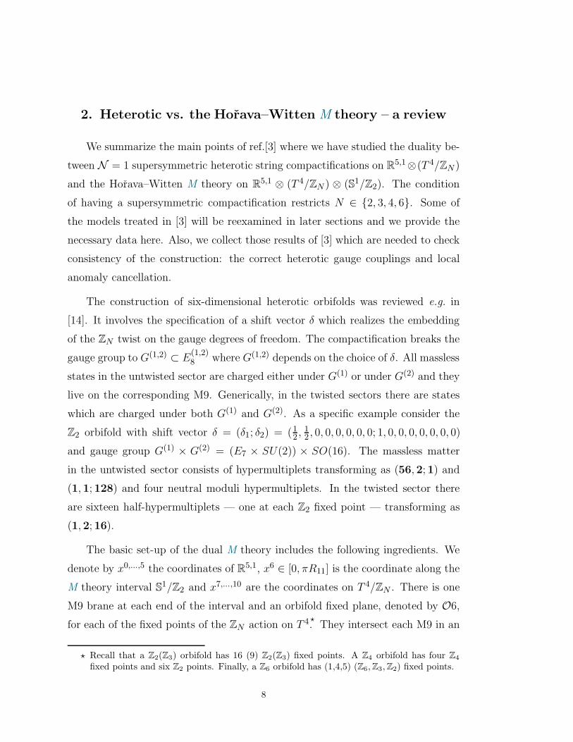
2. Heterotic vs. the Horava–Witten M theory – a review

We summarize the main points of ref.[3] where we have studied the duality be-

tween N = 1 supersymmetric heterotic string compactifications on R5,1⊗(T 4/ZN )

and the Horava–Witten M theory on R5,1 ⊗ (T 4/ZN ) ⊗ (S1/Z2). The condition

of having a supersymmetric compactification restricts N ∈ 2, 3, 4, 6. Some of

the models treated in [3] will be reexamined in later sections and we provide the

necessary data here. Also, we collect those results of [3] which are needed to check

consistency of the construction: the correct heterotic gauge couplings and local

anomaly cancellation.

The construction of six-dimensional heterotic orbifolds was reviewed e.g. in

[14]. It involves the specification of a shift vector δ which realizes the embedding

of the ZN twist on the gauge degrees of freedom. The compactification breaks the

gauge group to G(1,2) ⊂ E(1,2)8 where G(1,2) depends on the choice of δ. All massless

states in the untwisted sector are charged either under G(1) or under G(2) and they

live on the corresponding M9. Generically, in the twisted sectors there are states

which are charged under both G(1) and G(2). As a specific example consider the

Z2 orbifold with shift vector δ = (δ1; δ2) = (12 ,

12 , 0, 0, 0, 0, 0, 0; 1, 0, 0, 0, 0, 0, 0, 0)

and gauge group G(1) × G(2) = (E7 × SU(2)) × SO(16). The massless matter

in the untwisted sector consists of hypermultiplets transforming as (56, 2; 1) and

(1, 1; 128) and four neutral moduli hypermultiplets. In the twisted sector there

are sixteen half-hypermultiplets — one at each Z2 fixed point — transforming as

(1, 2; 16).

The basic set-up of the dual M theory includes the following ingredients. We

denote by x0,...,5 the coordinates of R5,1, x6 ∈ [0, πR11] is the coordinate along the

M theory interval S1/Z2 and x7,...,10 are the coordinates on T 4/ZN . There is one

M9 brane at each end of the interval and an orbifold fixed plane, denoted by O6,

for each of the fixed points of the ZN action on T 4.⋆

They intersect each M9 in an

⋆ Recall that a Z2(Z3) orbifold has 16 (9) Z2(Z3) fixed points. A Z4 orbifold has four Z4

fixed points and six Z2 points. Finally, a Z6 orbifold has (1,4,5) (Z6, Z3, Z2) fixed points.

8

I5, i.e. I5 = M9 ∩ O6.†

Compactification on S1/Z2 leads to the Horava–Witten

theory with an E8 factor on each end-of-the-world M9. Compactifying further on

T 4/ZN breaks the gauge group, as in the heterotic case, with G(1) confined to M91

and G(2) to M92. The charged matter corresponding to the untwisted sector of the

dual heterotic theory is localized either on M91 or on M92, depending on whether

they are charged under G(1) or G(2). The twisted matter states are localized on

the fixed planes O6 and, since they carry charge, on the end-on-the-world nine-

branes, i.e. on the I5’s. There seems to be no way to localize those states which

are charged under both G(1) and G(2).

The solution of the puzzle involves non-perturbative gauge fields which are

localized on the O6 planes. On a O6 plane corresponding to a An−1 singular-

ity one has the gauge group SU(n)np. The states corresponding to the Cartan

generators originate from the M theory three-form C and those corresponding to

the roots from M2 branes wrapping vanishing cycles. Supersymmetry requires

that these states are components of 7D vector multiplets. The presence of bound-

aries complicates the situation. In particular the boundary conditions of the 7D

fields at the ends of the interval have to be specified. Under Z2 : S1 → S1/Z2

eight supercharges are even and eight are odd and hence supersymmetry is bro-

ken 16–SUSY→8–SUSY. The 7D 16–SUSY vector multiplets decompose into a 6D

8–SUSY vector+hypermultiplet (V7D and H7D) with opposite — free vs. fixed —

boundary conditions. Another constraint is that in the heterotic picture, i.e. when

we collapse the interval to a point, there should be only the perturbative heterotic

states. This means e.g. for the Z2 model that the 7D fields do not have massless

zero-mods in 6D, i.e. neither V7D nor H7D has Neumann boundary conditions on

both ends.‡

Clearly, in the Z2 example, since there are no non-perturbative SO(16) gauge

† If we want to distinguish the two ends of the interval at x6 = 0 and x6 = πR11 we use sub-or superscripts ‘1’ and ‘2’, e.g. M91, etc..‡ In section 5 we consider models where some H7D components have zero modes. Nevertheless,

the condition that in the heterotic limit there are no additional states must and will besatisfied.

9

fields at our disposal, we have to place one half-hypermultiplet of the twisted sector

on each I52. The SU(2) charge it carries must be that of SU(2)np and it transforms

as (16, 2) of SO(16)(p)|M92× SU(2)(np)|O6. V7D must have Neumann boundary

conditions at I52 while at I51 the fields in V7D ‘lock’ to the SU(2) fields on M91,

i.e. they satisfy

Aµ(x6 = 0) = A10Dµ (x7,8,9,10 = 0) for same x0,...,5, µ = 0, . . . , 5 (1.2)

and likewise for the gauginos in the 6D vector multiplet. The SU(2) visible in

the heterotic description is the diagonal subgroup SU(2)het = diag[SU(2)p ×(SU(2)np)16]. The boundary conditions of H7D are opposite to those of V7D: Neu-

mann on I51 and Dirichlet on I52. At any given I5 only those 7D fields contribute

to the massless spectrum which satisfy Neumann boundary conditions there. The

main burden of the analysis of any given model is to determine the correct massless

spectrum at the I5s. We will see that this is a highly non-trivial problem in all but

the simplest models. The situation for the Z2 model is summarized in fig. (1.1).

Let us now give the evidence for this proposal which we have amassed in [3]

and which we had verified for several other models. In addition to reproducing

the correct perturbative heterotic spectrum, we showed that the correct heterotic

gauge coupling, which can be computed exactly, could be derived from the dual

M theory and also that the anomalies on each I5 cancel locally. Both checks rely

heavily on the set-up and will now be summarized in turn.

We start with the 6d gauge couplings. The gauge kinetic energy of the six-

dimensional low-energy effective N = 1 SYM theory is, in string frame, [15]

L ∼ 1

α′

∑

α

(vαe−φ + vα) trF 2

α . (2.1)

Here φ is the heterotic dilaton, e−φ =Vol(K3)λ2

hetα′2 , and λhet the heterotic string coupling

constant. The sum is over all gauge group factors. v and v are dimensionless

constants. For perturbative non-abelian gauge groups, v = 1 — it is, in fact, the

10

level of the Kac-Moody algebra — and v arises at one loop. For non-perturbative

gauge groups, on the other hand, v = 0 and v is fixed at tree level.

The coefficients v and v are related, via supersymmetry, to the coefficients of

the anomaly polynomial which must factorize to allow a Green–Schwarz mechanism

to cancel the anomaly. Factorizability of the anomaly polynomial in the form⋆

A ≡ 23 TrH−V (F4) − 1

6 tr(R2)× TrH−V (F2) +(

tr(R2))2

=

(

∑

i

vi tr(F 2i ) − tr(R2)

)

×(

∑

i

vi tr(F 2i ) − tr(R2)

)

.(2.2)

imposes the constraint

bα = 6(vα + vα), (2.3)

where bα is the coefficient of the one-loop beta-function of the d = 4, N = 2 SYM

theory that one obtains upon further compactification on T 2.

The M9 branes carry magnetic charges under k1,2 = n1,2−12 where n1,2 are the

instanton numbers which satisfy n1 + n2 = 24. In the orbifold limit the instantons

are located at the fixed points and can have fractional instanton number. The

relation between k and n follows from the Bianchi identity of the field strength of

C. If one integrates the anomaly polynomial of the heterotic theory over a smooth

K3 one derives v1,2 = 12k1,2, i.e. v1 + v2 = 0. In these compactifications there are

no non-perturbative gauge fields and we thus conclude that vp = k2 .

This does, however, not hold for the compactification on K3 orbifolds. In

fact, for the Z2 model one finds k1 = −4 and v(E7) = −2, v(SO(16)) = 2 but

v(SU(2)) = −2 + 16. The result for the SU(2) factor indicates that it is indeed

the diagonal subgroup of the perturbative SU(2) and 16 non-perturbative SU(2)’s

on the O6’s. Generally, for those group factors which have a perturbative and a

nonperturbative component, v = vp + vnp.

⋆ Here we have already used the necessary condition nH − nv = 244 for the GS mechanismto work.

11

Even though the non-perturbative fields do not contribute additional degrees

of freedom in the heterotic limit, they effect the heterotic gauge coupling via

1

g2het

=1

g2M9

+∑

i

1

g2O6

. (2.4)

The sum is over all those non-perturbative gauge groups which mix with the per-

turbative gauge group on M9. Combining this with 1g2M9

= 1α′

(

vol(K3)λ2

hetα′2 v + vp

)

and

vp = k2 we find for any factor G ⊂ E8 of the heterotic gauge group which mixes

with a non-perturbative gauge group G ⊂ SU(n) located at a Zn fixed plane,

1

g2G

=v

g2E8

+vnp

g2SU(n)

+ (1− loop), (2.5)

where the one-loop contribution is vp

α′ = k2α′ . Later we will compute 1

g2G

and use

eq.(2.5) to determine vnp for various models. The result depends on the details of

the mixing of perturbative and non-perturbative gauge groups which will turn out

to be highly non-trivial in the presence of U(1) factors. These values have to agree

with those derived from (2.2).

The second consistency check is local anomaly cancellation on each O6. In

the M theory description of the heterotic orbifold we have allocated all massless

fields (perturbative and non-perturbative) to the bulk (gravity and moduli) and the

various types of planes (M9, O6 or I5) which are present. The anomalies have to

cancel locally, i.e. on any such plane separately. In the bulk and on the O6 this is

automatic, they are odd-dimensional. On each of the two M9 branes, away from the

intersection planes I5, there are 16 supercharges and an entire E8 gauge group.

Anomaly cancellation works in exactly the same way as in the Horava–Witten

theory. The situation on the intersection planes I5, however, involves new features:

here supersymmetry is broken further to eight super-charges and the gauge group

is broken to a subgroup. The anomaly on the intersection planes gets contributions

from three sources: the quantum, inflow and intersection contributions. The total

12

anomaly polynomial is

A = A(Quantum) +A(inflow) +A(intersection) . (2.6)

Quantum contributions: they arise from the massless states which are charged

under the gauge group G6Dlocal operating at a particular I5. Fields residing in

the bulk, on the M9 planes, on the O6 plane which is bounded by the I5 plane

and the fields confined to I5 contribute. We will denote the multiplet content

of the charged M9 fields which contribute to the anomaly by Q10. This splits

in hypermultiplets and vector multiplets which contribute with opposite signs.

Likewise we introduce the notation Q7 and Q6 for the charged fields on O6 and I5which contribute to the anomaly. We also use Q = Q10+Q7 +Q6. The net number

of fields is denoted by dim(Q). Q7 gets contributions from H7D and V7D. Since

the boundary conditions are local and are not communicated across the interval,

the contributions of the 7D fields to the anomaly have to be distributed a priori

over the two I5 boundaries of O6. However, at each end only the components with

Neumann boundary conditions do actually contribute (but with a factor 12). Q6

consists of all the fields which are localized on the I5 plane. To determine Q10 we

have to distribute the M9 fields over all I5s on the same side of the interval. For

non-prime orbifolds one has to be careful. E.g. for a Z4 orbifold we first have to

subtract the contribution form the 6 Z2 fixed points and then distribute the rest

over the four Z4 fixed points. Q10 can be succinctly written as follows [3]: denote

by α the ZN generator whose action on E8 is realized by the shift vector δ. Then

for an ZN plane Q10 = −T (α)(248) where

T (x) =

x16 , N = 2 ,

x9 , N = 3 ,

x8 + x2

32 , N = 4 ,

x6 + x2

18 + x3

48 , N = 6 .

(2.7)

For the Z2 model of fig.(1.1) we have

13

Glocal1 = E10D

7 × SU(2)diag, Glocal2 = SO(16)10D × SU(2)7D,

α1(248) = (133, 1) + (1, 3)− (56, 2) and α2(248) = (120)− (128).

The local charged spectra are

Q(1)6 = ∅, Q

(2)7 = −1

2(1, 3), Q(1)10 = 1

16 [(56, 2)− (133, 1)− (1, 3)],

Q(2)6 = 1

2(16, 2), Q(1)7 = 1

2(1, 3), Q(2)10 = 1

16 [(128, 1)− (120, 1)]

from which dim(Q)1 = 0 and dim(Q)2 = 15 follows.

The last contribution to the quantum anomaly comes from the bulk fields.

They have to be distributed over all fixed planes at both ends of the interval.

One has again to be careful for non-prime orbifolds. In particular for the moduli

contribution one has to remember that ZN orbifolds have four moduli for N = 2

and two otherwise.

Combining all contributions one finally obtains the total quantum anomaly on

an ZN I5 plane of a ZN orbifold

A(quantum) =2

3TrQ F

4 − 1

6trR2 TrQ F

2

+1

360

(

dim(Q)− 122T (1)− 2ReT (e2πi/N )

)

trR4

+1

288

(

dim(Q) + 22T (1)− 2ReT (e2πi/N ))

(trR2)2 .

(2.8)

Inflow contributions: they arise from gauge variance of the 11d SUGRA action.

There is a contribution from a modified Bianchi identity and contributions arising

from Chern–Simons (CS) terms. Explicitly [4,3]

A(inflow) = −2g

3

(

1

8trR4 − 1

32(trR2)2

)

− g

2

(

trF 210 −

1

2trR2

)2

. (2.9)

Here F10 are the M9 gauge fields and g is the magnetic charge of the I5-plane

under consideration. The charges of all I5 planes on one side of the interval have

to satisfy the sum rule∑

g = k. For ZN orbifolds with N prime all I5 planes on

14

one side are equivalent and the magnetic charge of each of them is easily determined

once k is known. For the Z2 model this means that g1 = k1/16 = −1/4 = −g2.For N = 4, 6 one needs to take into account the magnetic charges of the Z2 and

(for N = 6) Z3 fixed planes. Their combined charge has to be subtracted from k

and the remainder has to be divided by the number of ZN fixed points.

Intersection contributions: they arise from the electric coupling of the O6 to the

three form C. This coupling leads to a 7D CS term on each of the O6 planes. One

finds [4,3]

A(intersection) =

(

trF 210 −

1

2trR2

)

×(

T (1) trR2 − trF 27

)

. (2.10)

Here F7 are the O6 gauge fields operating on I5=M9∩O6.

Anomaly cancellation requires that the coefficients of trR4, (trR2)2, trR2 and

of the term with pure gauge field dependence vanish separately. In particular,

absence of the irreducible trR4 term implies that

dim(Q ≡ Q6 +Q7 +Q10) = 30g +

152 for N = 2,

1219 for N = 3,

19 for N = 4,

53518 for N = 6.

(2.11)

Using this, the condition A ≡ 0 reduces to

A′ ≡ 23 TrQ(F4) − 1

6 tr(R2)× TrQ(F2) + (18g + 1

2T (1))(tr(R2))2

= 12g(

tr(F210D) − 1

2 tr(R2))2

+(

tr(F210D) − 1

2 tr(R2))

×(

tr(F27D) − T (1) tr(R2)

)

.

(2.12)

For all models that we will consider we check that (2.11) and (2.12) are satisfied

on each I5 plane separately.⋆

⋆ The relation between tr and Tr in various representations can be found e.g. in App. C of[3].

15

In addition to the Z2 model with gauge group (E7 × SU(2)) × SO(16) which

has accompanied us through this section, we also considered a Z3, a Z4 and a Z6

model in [3]. We will reconsider these models in view of the HW↔ type I′ duality

in section 7. Here we collect some basic data. Further details can be found in [3]

Z3 − orbifold with gauge group (E6 × SU(3))× SU(9)

shift vector: δ = (−23 ,

13 ,

13 , 0, 0, 0, 0, 0; 5

6 ,16 ,

16 ,

16 ,

16 ,

16 ,

16 ,

16)

untwisted matter: two moduli ⊕ (27, 3; 1) ⊕ (1, 1; 84)

twisted matter: 9× (1, 3; 9)

vE6= −3

2 , vSU(3) = −32 + 9; vSU(9) = +3

2

k1 = −3 = −k2 =⇒ gI51= −gI52

= −13

Glocal1 = E10D

6 × SU(3)diag, Glocal2 = SU(9)10D × SU(3)7D

Q(1)10 = 1

9 [(27, 3)− (78, 1)− (1, 8)], Q(1)6 = ∅, Q

(1)7 = 1

28

Q(2)10 = 1

9 [84− 80], Q(2)6 = (9; 3), Q

(2)7 = −1

28

Z4 − orbifold with gauge group (SO(10)× SU(4))× (SU(8)× SU(2))

shift vector: δ = (−34 ,

14 ,

14 ,

14 , 0, 0, 0, 0;−7

8,18 ,

18 ,

18 ,

18 ,

18 ,

18 ,

18)

untwisted matter: two moduli ⊕ (16, 4; 1, 1) ⊕ (1, 1; 28, 2)

twisted matter: 4×[

12(1, 6; 1, 2)⊕ (1, 4; 8, 1)

]

∣

∣

∣

Z4

⊕ 6×[

12(1, 6; 1, 2)⊕ 1

2(10, 1; 1, 2)

]

∣

∣

∣

Z2

vSO(10) = 0, vSU(4) = 0 + 4; vSU(8) = 0, vSU(2) = 0 + 6

k1 = k2 = 0 =⇒ gI51 = 14(0− 6× 1

4) = −38 = −gI52 (for Z4 planes)

Glocal1 = SO(10)10D × SU(4)diag, Glocal

2 = [SU(8)× SU(2)]10D × SU(4)7D

16

local spectrum at the Z4 intersection planes:

Q(1)10 = − 5

32[(45, 1) + (1, 15)] +

3

32(10, 6) +

1

16(16, 4)

Q(1)6 = ∅ , Q

(1)7 =

1

215

Q(2)10 = − 5

32[(63, 1) + (1, 3)] +

3

32(70, 1) +

1

16(28, 2)

Q(2)6 = (8, 1; 4) +

1

2(1, 2; 6) , Q

(2)7 = −1

215

Z6 − orbifold with gauge group (SU(6)× SU(3)× SU(2))× SU(9)

shift vector: δ = (−56 ,

16 ,

16 ,

16 ,

16 ,

16 , 0, 0;−5

6 ,16 ,

16 ,

16 ,

16 ,

16 ,

16 ,

16)

untwisted matter: two moduli ⊕ (6, 3; 2, 1)

twisted matter:[

(6, 1, 1; 9)⊕ 12(20, 1, 1; 1)

]

∣

∣

∣

Z6

⊕ 4× (1, 3, 1; 9)]∣

∣

∣

Z3

⊕ 5×[

12(20, 1, 1; 1)⊕ (6, 3, 1; 1)⊕ 2 (1, 1, 2; 1)

]

∣

∣

∣

Z2

vSU(6) = 1 + 1, vSU(3) = 1 + 4, vSU(2) = 1; vSU(9) = −1

k1 = −k2 = 2 =⇒ gI51= −gI52

= − 512 (for Z6 planes)

Glocal1 = [SU(3)× SU(2)]10D × SU(6)diag, Glocal

2 = SU(9)10D × SU(6)7D

local spectrum at the Z6 intersection planes:

Q(1)10 = − 35

144[(35, 1, 1) + (1, 8, 1) + (1, 1, 3)]

− 5

72(6, 3, 2) +

13

72(15, 3, 1) +

19

144(20, 1, 2)

Q(1)6 = ∅ , Q

(1)7 =

1

235

Q(2)10 =

13

7284− 35

14480

Q(2)6 = (9; 6) +

1

2(1; 20) , Q

(2)7 = −1

235

17

3. Explaining E8: HW ↔ I′ Duality

Ten-dimensional string theories are connected through a web of perturbative

and non-perturbative dualities; for a review, see e.g. [16]. One striking feature

is that if one studies the strong coupling limit of the type IIA theory, the string

coupling constant gets geometrized and parameterizes the size of an additional,

eleventh, dimension which is topologically a circle whose radius grows as the type

IIA coupling increases. The massless degrees of freedom of the type IIA theory

combine into representations of the eleven-dimensional Lorentz-group and their

dynamics is governed by eleven-dimensional supergravity. The strong coupling

limit of type I string theory is the heterotic SO(32) theory and vice versa; they are

S-dual to each other. The type IIB theory, which is of no interest for the discussions

in this paper, is self-dual. Finally, the strongly coupled heterotic E8×E8 theory is

also an eleven-dimensional theory, with the additional dimension being the interval

I ≃ S2/Z2. The gauge degrees of freedom are confined to the two ten-dimensional

boundaries, one E8 factor on each. The original arguments for this strong coupling

limit are due to Horava–Witten [1]. They are of purely kinematical nature and are

based on the requirement of local anomaly cancellation on each of the two boundary

planes. The theory in the bulk is straightforward — it is simply type IIA string

theory. The presence of boundaries has very non-trivial effects the result of which

is E8 SYM theory confined to each of its components. The dynamical origin of the

gauge fields, which are not present in the eleven-dimensional supergravity theory

stayed, however, mysterious. New insight came from the duality between the HW

theory and the type I′ theory, which we will now review. It provides an explanation

for the E8 gauge symmetry on the boundaries and also of its regular subgroups

some of which occur as gauge groups in T 4/ZN orbifold compactifications.

The results in this section are not new but we thought it worthwhile to collect

them as they are the basis of the brane constructions in the following sections. We

will, however, be brief and qualitative and refer to the cited literature for further

details.

18

The type IIB and type IIA string theories compactified on a circle are related by

T-duality [17,18] and so are their orientifolds, called type I and type I′, respectively.

The latter lives on R8,1 × S1/Z2. There is an orientifold eight-plane O8 of charge

−8 at each end of the interval. In addition, 16 D8 branes are required for charge

neutrality. Their positions along the interval are a priori arbitrary: they are T-dual

to the 16 Wilson-line moduli of the type I theory on S1. Generically the gauge

group is U(1)18 where sixteen factors live on the world-volumes of the sixteen D8

branes and the remaining two gauge bosons are the one-form ARRµ coupling to D0

charge and BNS9µ which couples to winding along x9.

⋆

Clumping branes together one can engineer any regular subgroup of SO(32):

a U(n) factor when n D8 branes coincide at a position away from the boundaries†

and a SO(2n) factor when n of them are located at a boundary. The massless

vector bosons (and their partners under supersymmetry) come from open strings

of zero length connecting the different branes and also, for branes located on one

of the O8 planes, the branes and their images under the space-time reflection

which, together with world-sheet parity reversal, generates the orientifold group.

Examples of such brane configurations with n = 8, 7, 6 will appear in sections 4,5

and 7, respectively. For instance, the Z3 orbifold model of § 5.1 requires the

following symmetric brane arrangement to engineer the perturbative gauge group

(SO(14)× U(1))(1) × (SO(14)× U(1))(2):

⋆ In this section x9 is the compact coordinate along S1 and S1/Z2. In the previous and alllater sections, where we compactify further on T 4/ZN , this coordinate is called x6.† If n1 branes sit at one position and n2 at another, the gauge symmetry is U(1)×SU(n1)×

SU(n2), etc..

19

0 b LL− bx9

O8

+7D

8SO

(14)

1D8

U(1

)

O8

+7D

8SO

(14)

1D8

U(1

)

x1,...,8

Dual to the M91 Dual to the M92

(3.1)

There is one feature of the type I′ vacua that we have not yet addressed which is

crucial for the heterotic↔type I′ duality. In contrast to the type I dilaton, which

is constant on S1, the type I′ dilaton varies across the interval. The inverse of

the type I′ coupling constant satisfies the one-dimensional Laplace equation with a

source of unit charge at the position of each D8 brane and a source of charge −8 at

each end of the interval. As a result is it a piecewise linear function whose gradient

jumps upon traversing a D8 brane. We will consider brane arrangements with

eight D8 branes sitting in the vicinity of each orientifold brane, say at x91,...,8 < b

and x99,...,16 > L− b. For b < x9 < L− b the dilaton is constant and if b/L << 1 it

makes sense to speak about the bulk value of the dilaton and the type I′ coupling

constant.

For generic D8 brane arrangements the coupling constant stays finite every-

where but for particular choices of their positions it diverges at one or both ends

of the interval; this will play an important role below. The dilaton is constant

across the entire interval if and only if eight D8 branes are located at each of the

two orientifold planes, i.e. if we have local charge neutrality and the (perturbative)

20

gauge group SO(16)× SO(16)× U(1)2.

This can, however, not be the whole story for the following simple reason.

The type I′T←→ type I

S←→ het.[SO()]T←→ het.[E × E]

S←→ Horava–Witten

duality chain means that we must be able to find e.g. E8 gauge group factors in

type I′. Perturbatively, neither type I not type I′ string theories allow exceptional

En gauge symmetries, hence we need a non-perturbative gauge group enhancement.

Since the duality chain from type I′ to het(E8×E8) involves an S-duality, we suspect

to find E8 in type I′ at strong coupling. This is true, also for various subgroups

such as E7 × SU(2) which will appear in the examples below.

A vacuum of the type I′ theory is specified by the value of the dilaton Φ0I′ ≡

ΦI′(x9 = 0) at the orientifold plane at x9 = 0, by the positions x9

i , i = 1, . . . , 16

of the D8 branes and by the size L of the interval. These parameters are mapped

under the duality to those characterizing a vacuum of het(SO(32)) compactified

on S1: to the (constant) heterotic dilaton Φh, the sixteen parameters of the Wilson

line on S1, A = (θ1, . . . , θ16) and to the radius Rh of the S1. The precise map of

the parameter spaces follows by comparing the low energy effective actions and

the masses of perturbative BPS states which are related by the duality. This was

first worked out in [19] and extended in [20,21,22,23,24,25]. The explicit relation

between the heterotic momentum and winding quantum numbers and the type I′

winding and D-particle number was established in [23].

The type I′ non-perturbative gauge symmetry enhancement, which should be

mapped to the perturbative regime in the heterotic theory, can now be verified.

The following qualitative discussion of a particular example shall illustrate this.

The precise values of the parameters may be found in the references cited above.

Choose the D8 locations such that seven of them are on the O8-plane at x9 = 0,

one at x9 = b and, for simplicity, the remaining eight at x9 = L, i.e. on top

of the second orientifold plane. For this brane arrangement ΦI′ has a constant

bulk value Φb for b ≤ x9 ≤ L and for any such Φb there is a range of values

for b where the type I′ coupling λI′ stays small throughout the interval. The

21

gauge group is SO(14)× U(1)× SO(16)× U(1)2. If, however, we move the single

D8 brane away from the orientifold plane at x9 = 0 to a critical position a(Φb),

the type I′ coupling diverges at x9 = 0 where the gauge theory on the world-

volume of the D8 branes becomes strongly coupled. If we now use the parameter

map we find that (a, L) map precisely to those values for the heterotic Wilson

line and Rh for which perturbative symmetry enhancement SO(14)× U(1) → E8

occurs.⋆

Choosing L appropriately guarantees that the heterotic coupling is small.

In the heterotic theory the additional massless states are BPS and carry winding

numbers ±1 and ±2. They are mapped [20,21,22,23,24] to type I′ D-particles.

More precisely, the heterotic states with winding number ±1 map to states with

D-particle number ±1/2. Such half D-particles necessarily sit at x9 = 0 from where

they cannot leave because of the Z2 orientifold symmetry. One also finds that they

are massless precisely for b = a. The fermionic zero modes of the string connecting

the half D-particle confined to the orientifold plane and the D8 branes provides the

64 spinor representation of SO(14) and the anti-D-particle the conjugate spinor

representation 64′. Their U(1) quantum numbers are ±1/2 respectively. The

heterotic states with winding 2 map to D-particles with particle number 1. They

should be viewed as threshold bound states of two half D0 particles stuck to the

orientifold plane. Massless states only arise from the 14 ⊂ 64×64 of SO(14). The

contribution to the massless spectrum from the D0 brane is another 14. The U(1)

quantum numbers are ±1. Altogether we have thus found those massless states

which are needed for the gauge symmetry enhancement.

In the region between a ≤ x9 ≤ L the dilaton is constant and the coupling

takes on its bulk value. Using the relations [19,1] λE ∼ L3/2/λ1/2I′ and RE ∼

√LλI′

where RE is the radius of the dual heterotic E8×E8 theory measured in heterotic

units lhet =√

α′het (L is measured in type I units) one sees that for L → ∞ with

λI′ (the bulk value) fixed, λE →∞ and RE →∞. Since in this limit a/L→ 0, all

eight D8 branes sit at the left boundary to which the gauge degrees of freedom are

⋆ Note that the position of the single D8 is frozen and no U(1) factor is associated with it.It has combined with SO(14) in the process of symmetry enhancement.

22

now confined. If we start with a symmetric (under x9 → L−x9) brane arrangement

we get symmetry enhancement at both ends of the interval. i.e. if we place seven

D8 branes on each orientifold plane, one D8 at x9 = a and one at x9 = L− a, we

get an enhanced E8 × E8 symmetry. This is the HW-theory compactified on S1,

i.e. M theory on R9 × S1 × (S1/Z2). The radius of the first S1 is controlled by λI′

via the relation λI′ ∼ R3/2.†

In section 4 we will study in detail a Z2 orbifold model with (perturbative)

gauge group (E7×SU(2))×SO(16). The required brane configuration is as follows:

0 a Lx9

O8

+6D

8

E7

λ=∞

2D8

SU

(2)

O8

+8D

8SO

(16)

x1,...,8

Dual to the M91 Dual to the M92

(3.2)

The SO(16) factor is straightforward: place eight D8 branes at x9 = L with ΦI′(L)

finite. As long as the coupling stays finite everywhere, the branes on the l.h.s.

of the interval give SO(12)× U(2). To get E7 we need to adjust the positions

of the two ‘outlier’ D8 branes such that the coupling becomes infinite at x9 = 0.

The fact that two D8 branes must be placed at a critical distance a means that

their center-of-mass motion is frozen and the gauge group on their world-volume is

† Similarly, starting with brane arrangements for other gauge groups G(1) ×G(2) ⊂ E8 × E8

and keeping fixed the bulk value λI′ , one finds that in the limit L→∞ all branes sit at theboundaries. Their position moduli have become Wilson lines on the S1.

23

SU(2) rather than U(2). With the help of the map between type I′ and heterotic

parameters we can again verify that this brane arrangement maps to the critical

radius and Wilson line on the heterotic side where states with winding numbers ±1

and ±2 become massless. Again this corresponds to a half D0 brane stuck on O8

whose fermionic zero modes provide the 32 and 32′ of SO(12) with U(1) charges

±1/2 and the 1 component of D0-D0 and D0-D0 threshold bound states with U(1)

charges ±1 [23,24]. These states, together with those from the 8-8 strings, provide

the adjoint representation of E7.

The generalization to gauge groups En × SU(9 − n) is straightforward. They

involve the SO(2n − 2) × U(1) → En enhancement. For 0 < n < 7 only wind-

ing states with winding number ±1 become massless in the heterotic dual and

consequently only the fermionic zero modes of half D0 and D0 branes contribute.

They provide the two spinor representations of SO(2n− 2) which in all cases are

sufficient to complete the adjoint of En.

At this point it seems appropriate to comment on the mixing of U(1) factors

[24]. As already said, in addition to the perturbative open string gauge group there

are two U(1) factors with gauge bosons ARRµ and BNS

9µ originating from the bulk

fields of the type I′ theory. As long as the dilaton is constant across the whole

interval, these do not mix with the open string gauge group. However, as we move

D8 branes into the interval, mixing sets in. E.g. the U(1) group associated with a

single D8 brane outside an orientifold plane with SO(14) gauge group mixes with

the two additional U(1) factors where the mixing depends of the distance a from the

orientifold plane. The U(1) which is involved in the SO(14)×U(1)→ E8 symmetry

enhancement is the U(1) that one gets at a. The mixing is well understood in the

dual heterotic theory where it is caused by switching on Wilson lines. So, in

principle, one should be able to push it through the duality chain to the type I′

theory. However we have not attempted to done so.

In § 7.3. we will reconsider the T 4/Z3 model of ref. [3] where the E(1)8 is broken

down to E6 × SU(3) and the E(2)8 down to SU(9). Given the brane engineering

24

tools at hand the first factor is straightforward to obtain in type I′, but we need

to introduce a new tool in order to explain the SU(9) factor. Clearly, we can

never get an SU(9) group with eight D8 branes only; cf. however the discussion

in [24]. To understand how it can arise, we need to elaborate further on the

properties of the type I′ theory at infinite coupling. In refs.[25,12,13,26] three

different arguments are exploited: (i) heterotic ↔type I′ duality; (ii) the world-

volume theory on a D4 probe in the background of D8 branes and O8 planes in

type I′; (iii) M theory compactification of Calabi-Yau threefolds. Here we will

restrict ourselves to a review of (i) since it is closest to the spirit of this paper.

Consider the heterotic Wilson line A = (015, θ16). For a fixed coupling constant the

moduli space of the heterotic theory is a strip in the (Rh, θ16) plane bounded by

1 ≥ θ16 ≥ 0 and R2h ≥ 2(1− θ2

16/2). At a generic point on the strip the symmetry

is SO(30)× U(1)3. On the boundaries θ16 = 0 and θ16 = 1 the gauge symmetry

is enhanced to SO(32)× U(1)2. Along the R2h boundary the generic symmetry is

SO(30) × SU(2) × U(1)2. However, on the lines θ16 = 0, 1/2, 1 the symmetry is

enhanced to SO(32) × SU(2) × U(1), SO(30) × E2 × U(1) and SO(34) × U(1),

respectively.

In the dual type I′ description, the heterotic Wilson line corresponds to having

15 D8 branes at x9 = 0 and one at a position 0 ≤ x9 ≤ L which is determined by

θ16. In particular, θ16 = 1/2 maps to x9 = L. Due to the invariance under θ16 →(1 − θ16) – they lead to identical brane configurations in the perturbative type I′

theory – the domain of the heterotic moduli space which maps to the perturbative

type I′ theory should be restricted to R2h ≥ 2(1−θ2

16/2) and R2h ≥ 2(1− 1

2(1−θ16)2).In particular the point with enhanced SO(34)×U(1) gauge symmetry where R2

h = 1

is not mapped to the perturbative type I′ theory. In [13] an extension of the type I′

description to the non-perturbative regime was proposed whereby a map of the

complete heterotic moduli space to a brane configuration was achieved. It assumes

that for θ16 = 1/2 and infinite coupling at x9 = L an additional D8 brane can be

extracted from the orientifold plane. For θ16 > 1/2 the original and the new D8

branes have left the O8 plane, leaving behind an orientifold plane of charge −9

25

which we will henceforth refer to as an O8∗ plane. The relative distance between

these two planes is controlled by R2h and they coincide for R2

h = 2(1− θ216/2). In

particular for θ16 = 1 and R2h = 1 they have both joined the other 15 D8 branes

at x9 = 0 and the gauge symmetry is enhanced to SO(34)×U(1). In the presence

of an O∗ brane and the additional D8 brane the variation of the inverse coupling

constant across the interval will change accordingly.

There is no gauge symmetry associated with an O∗ plane. In fact, if we put

(8+1) D8 branes at the critical distance from the orientifold plane we realize the

n = 0 member of the series En×SU(9−n) where E0 denotes the trivial symmetry

group of the En series.

We are now ready to give the dual type I′ brane arrangement which reproduces

the perturbative gauge group of the T 4/Z3 orbifold of [3]:

x90 a1 L− a2 L

O8

+5D

8

E6

λ=∞

3D

8SU

(3)

9D

8SU

(9)

O8∗

λ=∞

E0

Dual to the M91 Dual to the M92

x1,...8

(3.3)

Thanks to the −9 charge of this plane, we put nine rather than eight coincident

D8 branes at the critical location L− a2 where they carry an SU(9) SYM on their

world-volume.

26

4. Brane Duals of the HW Orbifolds

All massless charged particles in the untwisted sector of a heterotic orbifold are

made out of 10D E8 × E8 SYM fields. The dynamical origin of these fields in the

Horava–Witten M theory is rather Mysterious, but in the previous section we saw

an explanation of this Mystery in terms of the dual type I′ superstring theory. In

this section, we address HW Mysteries of the twisted sectors of heterotic orbifolds;

again, our explanation involves HW ↔ type I′ duality. §4.1 below relates the O6

orbifold fixed planes in the 11D bulk of the HW brane world to the D6 branes of

the superstring theory; the end-of-the-world M9 branes are addressed in §4.2 and

the O6/M9 intersections in §4.3–4.

4.1 Orbifold Planes, D6 branes and Taub–NUTs

Massless states in twisted sectors of a heterotic orbifold live in the immediate

vicinity of the appropriate fixed plane and don’t care for the overall geometry of the

T 4/ZN space. As far as these states are concerned, we may replace the toroidal

orbifold with the non-compact space C2/ZN or any other space with a similar

orbifold singularity; for supersymmetry’s sake, this replacement space should have

SU(2) holonomy, but there are no other restrictions. For simplicity, we would like

a non-compact replacement space with a simple flat asymptotics; in order to make

contact with the type I′ theory discussed in the previous section, we choose the

R3 × S1 flat asymptotics [27] instead of the R4.

The SU(2) holonomy and the R3× S1 asymptotics immediately lead us to the

multi–Taub–NUT geometry of N Kaluza–Klein magnetic monopoles,

ds2 = V (x)dx2 +

(

dy − A(x)dx)2

V (x), (4.1)

where y ≡ y + 2πR is a periodic coordinate of some radius R,

∇×A(x) = ∇V (x) and V (x) = 1 +N∑

i=1

(R/2)

|x− xi|. (4.2)

27

The multi–Taub–NUT geometry is smooth when all the monopoles are located at

distinct points xi in the 3D space but develops a C2/Zk orbifold singularity when

k monopoles become coincident. In particular, when all N monopoles sit at the

same point, the multi–Taub–NUT geometry is an orbifold of the simple Taub–NUT

space,

TNN = TN1/ZN for ZN : (x, y) 7→ (x, y + 2πRN ). (4.3)

In the large radius limit R → ∞ the local curvature of the Taub–NUT be-

comes negligible and the multi–Taub–NUT geometry approximates the flat orbifold

TNN ≈ C2/ZN .

The main idea of this section is to replace the T 4/ZN orbifold with the TNN

geometry and then to make the Kaluza–Klein radius R small rather than large;

this is legitimate because the massless twisted spectrum of the orbifold is chiral

and hence independent of continuous parameters such as R. In the 11D bulk of the

HW brane world, the Kaluza–Klein compactification of the M theory on a circle is

dual to the type IIA superstring theory in 10 flat spacetime dimensions; for small

R, the superstring is weakly coupled. In the type IIA context, each KK monopole

of the multi–Taub–NUT geometry (4.1) becomes a D6 brane [Townsend] located at

(x7, x8, x9) = xi and spanning x0, . . . , x6. N coincident monopoles of the singular

TNN space become N coincident D6 branes; the open strings beginning and ending

on these branes give rise to a U(N) SYM theory in the D6 world volume.

From the dual M theory point of view, an open string connecting two distinct

D6 branes (corresponding to an off-diagonal element of the U(N) matrix) is an M2

membrane or anti-membrane wrapped around a 2–cycle of the multi–Taub–NUT

geometry whose area (and hence the particle’s mass) vanishes when the two KK

monopoles coincide in space. The diagonal matrix elements — the open strings

beginning and ending on the same D6 brane — give rise to the moduli multiplets

associated with locations of the corresponding D6 branes; from the M point of

view, they are the location moduli xi of the individual KK monopoles. Among

these moduli, the positions of the KK monopoles relative to each other are moduli

28

of the resolutions of the C/ZN orbifold singularity, but the overall center-of-mass

motion of the singularity is an artifact of the non-compactness of the multi–Taub–

NUT geometry. This center-of-mass motion — responsible for the abelian U(1)

factor of the U(N) gauge group — has nothing to do with the twisted sector of

the orbifold. Indeed, in the compact T 4/ZN theory, the moduli responsible for

the center-of-mass motions of complete un-resolved singularities belong to the un-

twisted sector of the orbifold.

Therefore, on the type IIA side of the duality, the U(1) ⊂ U(N) associated

with the center-of-mass motion of the whole stack of N coincident D6 branes is

an artifact of replacing the T 4/ZN geometry with TNN and has nothing to do

with the twisted sector of the orbifold. In our subsequent analysis of the twisted

sectors and their brane duals, we shall disregard such abelian factors of the D6

gauge groups and focus on the non-abelian SU(N) SYM fields.

4.2 Taub–NUTs and Branes at the End of the World

In the complete Horava–Witten context — including both the 11D bulk and

the two end-of-the-world boundary M9 branes — the KK reduction leads to type I′

rather than type IIA superstring (cf. section 3) and the D6 branes dual to the O6

orbifold planes span the finite dimension of the type I′ theory. Let us dub this

finite dimension x6 while (x0, . . . , x5) denote the 6D Minkowski space. In the HW

theory, (x7, . . . , x10) are coordinates of the T 4/ZN orbifold or its TNN replacement;

in the small-radius limit of the multi–Taub–NUT geometry, we lose the x10 = y

coordinate to the KK reduction and the monopoles become D6 branes located at

(x7, x8, x9) = xi = 0. This naturally raises The Question: “What happens to the

D6 branes when they reach the ends of the world at x6 = 0 and x6 = L?

Before we answer this question however, we must first clarify what happens

at x6 = 0, L away from the D6 branes. Let us start by considering the effect of

orbifolding on the end-of-the-world M9 branes of the Horava–Witten theory. For

the flat toroidal orbifold T 4/ZN , at generic points of either M9 brane one has locally

29

unbroken E8 gauge symmetry and 16 supercharges. Only at the I5 = M9 ∩ O6

intersections with the fixed planes of the orbifold action there is a local effect: The

gauge symmetry is broken down to the commutant of the α : ZN 7→ E8 twist

and SUSY down to 8 supercharges. The multi–Taub–NUT space is not flat (apart

from the singularity) but it flattens out at large distances from the coincident

monopoles, hence for |x| ≫ R we have effectively unbroken local E8 symmetry and

all 16 supercharges. Or rather, the local symmetry on the M9 brane is unbroken

E8 — but the KK reduction of the x10 coordinate introduces Wilson lines into the

picture. Hence, the effective theory on the 9D boundary brane of the 10D brane

world has a reduced gauge symmetry.

In a generic KK compactification on a circle, the Wilson lines would be quite

arbitrary, but in the TNN compactification (4.3) the asymptotic SI51 circle at

x → ∞ is topologically equivalent to the noncontractable loop around the ZN

orbifold singularity at x = 0. As a stand-in for the T 4/ZN orbifold, the TNN

compactification should have Fµν = 0 outside the singularity itself, hence topolog-

ically equivalent loops have equivalent Wilson lines. Furthermore, the non-trivial

ZN Wilson line around the singularity is precisely the action of the orbifolding

symmetry on the E8 gauge fields; again, we should copy this action from the par-

ticular T 4/ZN heterotic orbifold model under consideration. The bottom line of

this argument is that the Wilson line around the KK circle should be precisely the

α : ZN 7→ E8 twist of the heterotic orbifold; this is not an inherent constraint of the

Horava–Witten theory, but any other choice would spoil the equivalence between

the T 4/ZN and the TNN twisted sectors.

In the dual type I′ superstring theory [19] the KK Wilson lines manifest them-

selves as brane arrangements within the O8 + 8D8 boundary stack at each end of

x6, cf. section 3. From the type I′ point of view, such arrangements have abso-

lutely no relation to the D6 branes at x = 0 which are dual to the orbifold fixed

plane. However, in order to make use of HW↔ I′ duality in the orbifold context,

we must engineer the specific brane arrangement in which the gauge group of the

9D SYM living on each boundary is precisely the commutant of the ZN action in

30

the appropriate E8 in the specific heterotic/HW orbifold under consideration. For

example, for the T 4/Z2 orbifold in which E(1)8 is broken to E7 × SU2 and E

(2)8

is broken to SO16 we should engineer the branes to yield E7 × SU2 near x6 = 0

and SO16 near x6 = L. As discussed in section 3, this means the following brane

layout:

0 a Lx6

O8

+6D

8

E7

λ=∞

2D8

SU

2

O8

+8D

8SO

16

2D6

SU2

? ?

Dual to the M91 at x6 ≈ 0 Dual to the M92 at x6 = Lx

7,8

,9 (4.4)

where the location a of the two ‘outlier’ D8 branes at the left end of the world is

tuned such that the x6–dependent string coupling λ diverges at x6 = 0, hence the

gauge symmetry enhancement from SO(12)× U(2) to E7 × SU(2)

4.3 Ends of D6 Branes: The O8 Terminus

The two elliptic blots on figure (4.4) denote the two Mysterious I5 regions of

the HW orbifold where the O6 fixed plane intersects the end-of-the-world M9s.

In the dual type I′/D6 picture, these regions contain brane junctions amenable

to string-theoretic analysis — which will finally reveal the physical origin of the

boundary conditions for the 7D fields discovered in ref. [3]. Let us start with the

yellow junction on the right side of fig (4.4) where all 8 D8 branes coincide with

the O8 orientifold plane at x6 = L.

31

More generally, consider a junction of N D6 branes terminating on an O8

orientifold plane accompanied by k D8 branes [28]. The orientifold plane acts

like a mirror; combining the branes on figure (4.4) with their reflections under

x6 → 2L − x6, we have a stack of 2k coincident D8 branes at x6 = L crossed at

the right angle with a stack of N coincident D6 branes at x = 0.

N D6

U(N)

kD8 + kD8

U(2k)→ SO(2k)

(4.5)

Before the orientifold projection, the open strings connecting these D branes pro-

duce the following massless particles: U(2k) gauge bosons and their 9D, 16–SUSY

superpartners from the 88 strings; U(N) gauge bosons and their 7D, 16–SUSY su-

perpartners from the 66 strings; 6D, 8–SUSY hypermultiplets in the bi-fundamental

(N, 2k) representation of the gauge group from the 68 strings. Note that only 8 out

of 32 supercharges of the type II superstring survive at the D8–D6 brane junction.

Locally near x6 ≈ L, the O8 orientifold projection Ω reverses L−x6, transposes

the Chan–Patton indices of open strings and breaks half of the supercharges. For

the 7D massless modes of the 66 open strings, the three effects are independent,

thus Ω = Ω1Ω2Ω3 where:

• Ω1 = ±1 is the parity of the spatial wave function, ψ(x6−L) = Ω1ψ(L−x6).

In x6 ≤ L terms, this translates into the boundary conditions for the wave

functions — and hence for the corresponding fields — at the x6 = L end of

the world: Neumann BC for the Ω1–positive fields and Dirichlet BC for the

Ω1–negative fields.

32

• Ω2 transposes the D6 Chan–Patton indices; in N ×N matrix terms (for the

two D6 indices of a 66 string), the symmetric matrices are Ω2–positive and

the antisymmetric matrices are Ω2–negative.

• Ω3 is the 6D chirality of the 8–SUSY supermultiplet; for the O8− orientifold,

the vector multiplets are Ω3 positive and the hypermultiplets are Ω3 negative.

The states surviving the projection have Ω = +1 and hence Ω1 = Ω2Ω3. Thus,

⋆ 7D fields with Neumann (free) boundary conditions at x6 = L comprise (6D)

vector multiplets for the symmetric N ×N matrices and hypermultiplets for

the antisymmetric matrices.

⋆ The fields with Dirichlet boundary conditions comprise vector multiplets for

the antisymmetric matrices and hypermultiplets for the symmetric matrices.

Note that the local gauge symmetry at x6 = L must make sense group theoreti-

cally, hence the symmetric N × N matrices must form a closed Lie algebra; such

an algebra is called symplectic and denoted Sp(N/2); it exists for even N only.

Consequently, the number N of D6 branes terminating at the same generic point

on an O8− orientifold plane must be even.

In the Sp(N/2) terms, the multiplet structure of the 7D fields includes one

symmetric tensor multiplet , one irreducible antisymmetric tensor multiplet ˜ =

− 1, and one singlet — which is responsible for the center-of-mass motion of the

D6 branes and irrelevant for the HW orbifold problem. Thus, as far as the 7D

SU(N) SYM fields living on a ZN O6 plane of a HW orbifold are concerned, the

type I′/D6 dual theory provides the following boundary conditions:

1. Locally, at x6 = L, the 7D gauge group is partially broken from SU(N) down

to Sp(N/2);

2. (6D) vector multiplets in the adjoint of the Sp(N/2) and hypermultiplets

in the ˜ have Neumann boundary conditions at x6 = L;

3. the remaining vector multiplets in ˜ and hypermultiplets in the have

Dirichlet boundary conditions at x6 = L.

33

The action of the orientifold projection on the 88 and 68 open string states is

less complicated. The 88 open strings are precisely as in the type I′ superstring

without the D6 branes: The O8− orientifold projection breaks the 9D gauge group

down to SO(2k) but all 16 supercharges remain unbroken away from x = 0. At

the junction, there are only eight supercharges and the massless modes of the 68

open strings form 6D hypermultiplets. The orientifold projection removes precisely

one half of each hypermultiplet, leaving us with half-hypermultiplets in the bi-

fundamental (N, 2k) representation of the net Sp(N/2)×SO(2k) gauge symmetry

at the brane junction; ‘fortunately’, this representation is pseudo-real so it allows

half-hypermultiplets.⋆

Finally, let us return to the specific example ofN = 2, k = 8 dual to the SO(16)

side of the Z2 HW heterotic orbifold. Because Sp(1) = SU(2), the 7D SU(2) gauge

group remains completely unbroken at the x6 = L terminus; all 3 vector multiplets

satisfy Neumann boundary conditions and all 3 hypermultiplets satisfy Dirichlet

boundary conditions. Furthermore, there are ‘twisted’ massless fields localized at

the junction, namely half-hypermultiplets in the (2, 16) representation of the net

locally visible gauge symmetry SU(2)× SO(16).

O8

+8D

8SO

16

2D6

SU2

Glocal = SU(2)× SO(16),

7DV = 3,

7DH = 0,

6DH = 12(2, 16).

(4.6)

⋆ Obviously, this pseudoreality is not an accidental ‘good fortune’ but a consistency constrainton the orbifold projection Ω. This is precisely the constraint which requires Ω to selectopposite (anti) symmetrizations for the D8 and D6 Chan–Patton indices, hence the netgauge group is either SO(2k)×Sp(N/2) (the O8

− projection) or Sp(k)×SO(N) (the O8+

projection) but never Sp(k)× Sp(N/2) or SO(2k)× SO(N).

34

Note that these are precisely the boundary conditions and the local fields we found

in ref. [3] to occur at the I52 intersection plane of the dual HW orbifold. In the

HW theory, this combination of boundary conditions and local fields was a solution

of several kinematic constraints but its dynamical origin remained a Mystery; this

particular Mystery is now solved in terms of the dual type I′/D6 superstring model.

4.4 D6 Branes Terminating on D8 branes and the Diagonal Gauge

Groups.

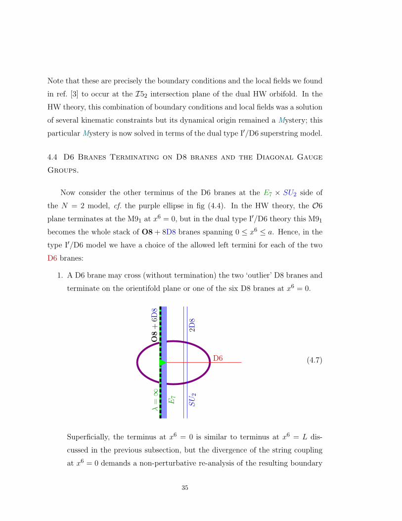
Now consider the other terminus of the D6 branes at the E7 × SU2 side of

the N = 2 model, cf. the purple ellipse in fig (4.4). In the HW theory, the O6

plane terminates at the M91 at x6 = 0, but in the dual type I′/D6 theory this M91

becomes the whole stack of O8 + 8D8 branes spanning 0 ≤ x6 ≤ a. Hence, in the

type I′/D6 model we have a choice of the allowed left termini for each of the two

D6 branes:

1. A D6 brane may cross (without termination) the two ‘outlier’ D8 branes and

terminate on the orientifold plane or one of the six D8 branes at x6 = 0.

O8

+6D

8

E7

λ=∞

2D8

SU

2

D6 (4.7)

Superficially, the terminus at x6 = 0 is similar to terminus at x6 = L dis-

cussed in the previous subsection, but the divergence of the string coupling

at x6 = 0 demands a non-perturbative re-analysis of the resulting boundary

35

conditions and local 6D fields. As of this writing, the physics of such λ =∞terminal junctions remains somewhat mysterious, but the net effect may be

inferred from duality considerations; we shall return to this issue in section 7.

2. Alternatively, a D6 brane may terminate on one of the two outlier D8 branes

at x6 = a without extending all the way to the true ‘end of the world’ at

x6 = 0.O

8+

6D8

E7

λ=∞

2D8

SU

2

D6 (4.8)

It turns out that both D6 branes of the type I′/D6 model dual to the T 4/Z2

heterotic orbifold should terminate in this manner at x6 = a.

Indeed, for the heterotic orbifold with E8×E8 broken to[

E7×SU(2)]

×SO(16),

all massless twisted states are E7 singlets. In terms of the dual type I′/D6 model,

this implies spatial segregation between the D6 branes and the E7 gauge fields

living at x6 = 0 — in other words, terminating the D6 branes at x6 = a > 0.

Furthermore, we need to explain the Mystery of the locking boundary conditions

(1.2) for the SU(2) fields of the HW orbifold; in the dual type I′/D6 terms, these

boundary conditions become

A7Dµ (x6 = a) = A9D

µ (x = 0). (4.9)

We shall see momentarily that such gauge field locking follows from each of the

two D6 branes at x = 0 terminating on a separate outlier D8 brane at x6 = a

36

according to following figure:

O8

+6D

8

E7

λ=∞

2D8

SU

2

2D6

SU(2)(4.10)

Proper understanding of the D6–D8 brane junctions (as opposed to simple

brane crossings) involves inter alia the mechanical tension of the D–branes. A

D6 brane pulls on the D8 brane on which it ends and bends it out of planarity;

consequently, each of the two outlier D8 branes on figure (4.10) is located at

x6 = a +α′

|x| (4.11)

instead of simply x6 ≡ a. At the junction itself (x = 0) the D8 branes are singular

and the quantum string effects become important.

The simplest way to understand these effects is via T-duality. Let us compactify

one of the transverse coordinates of the blue D8 branes, e.g. x7 on a large circle

of radius R7, then T-dualize x7 → x7. This duality turns the D8 branes into

D7 branes spanning x0, . . . , x5 and x8, x9 with transverse coordinates x6 and x7.

Consequently, the co-dimension of the junction in the brane reduces from 3 down

to 2, hence the bending of the brane [29] by the sideways pulling force becomes

logarithmic,

x6 = a +α′

R7log

α′/R7√

(x8)2 + (x9)2(4.12)

instead of the Coulomb shape (4.11). The bend D7 brane preserves 8 out of 32

supercharges of the (T-dual) type IIB superstring; to make SUSY manifest, it is

37

convenient to introduce complex coordinates

(x6 − a) + ix7 = R7 × w, x8 + ix9 = R7 × u, (4.13)

where R7 = α′/R7 is the radius of the T-dual x7 circle; note that w is a cylindrical

coordinate, w ≡ w + 2πi. In terms of these complex coordinates, the D7 branes

span a holomorphic curve

w = log1

u. (4.14)

The D6 branes at x = 0 are mapped by the T-duality onto D7′ branes span-

ning the x7 coordinate in addition to the x0, . . . , x6; the x8, x9 coordinates remain

transverse; in terms of the complex coordinates (4.13), the D7′ branes are located

at u ≡ 0 ∀w.

Now consider a single D6 brane terminating on a single D8 brane. The T-dual

of this picture is a junction between a D7′ and a D7 brane. Because of the D7

brane bending (4.14), this junction is located somewhat to the right of x6 = a, i.e.

at Rew > 0. Re-writing eq. (4.14) as

u = e−w, (4.15)

we see that for Rew > 0 the D7 brane rapidly asymptotes to u ≡ 0. Consequently,

the D7 brane smoothly connects to the D7′ brane without any discontinuity. In

other words, the whole complex of the D8 brane and the D6 brane terminated on

it is T-dual to a single curved D7 brane spanning (4.15).

As a corollary, the complex of two coincident D6 branes terminated on two

coincident D8 branes in a one-on-one manner depicted on fig (4.10) is T-dual to

a single pair of coincident smoothly curved D7 branes. The U(2) SYM generated

by the 77 open strings of the T-dual theory has exactly one local U(2) gauge

symmetry at every point of the D7 world-volume. By T-duality, this means that

the (4.10) complex of 2 D6 and 2 D8 branes has exactly one local U(2) gauge

38

symmetry at every point of the D6 + D8 world volume, including the junction

point (x6 = a,x = 0). Therefore, at the junction point, the U(2) gauge fields

living on the D6 world-volume and the U(2) gauge fields living on the D8 world-

volume must satisfy the locking boundary condition (4.9).

In the type I′/D6 context, the locking boundary conditions (4.9) apply to

the U(2)7D × U(2)9D → U(2)diag gauge theory involved in the brane junctions.

From the M theory point of view however, the U(1) center of the 9D U(2) is an

artifact of the KK reduction of the HW theory to the type I′ superstring and,

likewise, the U(1) center of the 7D U(2) is an artifact of the multi–Taub–NUT

geometry replacing the T 2/Z2 orbifold. Hence in the HW orbifold context, the

Mysterious locking boundary conditions (1.2) should apply to the simple SU(2)7D×SU(2)10D → SU(2)diag gauge theories only.

Next, consider the supermultiplet structure of the diagonal SU(2) SYM theory.

Locally, at every point of the T-dual D7 world volume there are 16 unbroken su-

persymmetries but the dimensional reduction to the effective 6D theory preserves

only 8 of the supercharges. Consequently, the 6D vector multiplets and hyper-

multiplets have different wave functions on the holomorphic curve (4.15). The

T-dual wave functions on the D8–D6 brane junction are governed by the boundary

conditions at the junction point. Hence, by T-duality, the hypermultiplets have

different boundary conditions than the vector multiplets; specifically, given the

Dirichlet-like locking boundary conditions for the vector multiplets, it follows that

the hypermultiplets satisfy the free (Neumann) boundary conditions. That is, at

the junction point, there are both 9D and 7D hypermultiplets (each in the adjoint

3 representation of the diagonal SU(2) gauge group) and both are free to take

whatever values they like independently of each other.

Actually, we do not need T-duality to establish the Neumann boundary con-

ditions for the 7D hypermultiplets at the brane junction. (The 9D fields are au-

tomatically free since they cannot possibly be pinned down at a codimension 3

junction, whatever the junction physics.) All we need to know is that at x6 = a,

39

each of the two D6 branes is free to move its attachment point to the D8 brane in

the three transverse dimensions (x7, x8, x9) = x independently of the other brane.

Note that from the 7D world-volume point of view, the transverse coordinates of

the two D6 branes are scalars in the 7D, 16–SUSY vector multiplets in the Car-

tan U(1)2 subalgebra of the U(2) SYM theory. Therefore, the freedom to move

the attachment points of the D6 branes in the transverse directions implies free

(Neumann) boundary condition for the corresponding scalar fields. In the 6D, 8–

SUSY terms, these scalars belong to hypermultiplets, hence thanks to SUSY and

the non-abelian gauge symmetry, we must have Neumann boundary conditions for

the entire hypermultiplets in the adjoint representation of the 7D gauge group.

Finally, consider the 68 open strings at the D6–D8 brane junction. In principle,

such open strings may have massless modes localized at the 6D junction plane.

However, the T-duality shows that this does not happen. Indeed, consider the pair

of curved D7 branes dual to the junction in question. The holomorphic curve (4.15)

has an arbitrary scale R7 which can be made large if desired, hence the 77 opens

strings have no inherently stringy 6D massless modes trapped in the junction area.

Hence the only possible localized 6D massless fields are the normalizable zero modes

of the 8D massless fields — the U(2) SYM — but the non-compact curve (4.15)

does not have any normalizable zero modes. Altogether, the 77 open strings of

the T-dual theory do not have any localized zero modes corresponding to massless

6D fields, and by T-duality, the 68 strings of the type I′/D6 model — or for that

matter, the 66 or 88 strings — do not produce any massless 6D fields trapped at

the junction.

To summarize, the brane junction depicted on fig. (4.10) correctly reproduces

the Mysteries at the E7 × SU(2) terminus of the Z2 fixed 7–plane of the HW

orbifold: The SU(2)7D×SU(2)9D gauge symmetry is broken to the diagonal SU(2)

by the locking boundary conditions (4.9) while the E7 gauge fields do not couple

to the massless twisted states; the hypermultiplets satisfy the Neumann boundary

conditions at the junction; and there are no massless 6D fields localized at this

junction.

40

5. Brane Duals of Orbifolds with

Broken 7D Gauge Symmetries

In the previous section we focused on the simplest example of the HW heterotic

orbifold, namely the T 4/Z2 with E(1)8 broken down to E7×SU(2) and E

(2)8 down to

SO(16); the type I′/D6 brane dual of this model has D–branes arranged according

to

0 a Lx6

O8

+6D

8

E7

λ=∞

2D

8SU

(2)

O8

+8D

8SO

16

2D6

SU2

Dual to the M91 at x6 ≈ 0 Dual to the M92 at x6 = L

x7,8

,9 (5.1)

In this section, we shall brane engineer the dual models for more complicated Z3

and Z4 orbifolds in which massless twisted states are charged under abelian factors

of the broken E8 × E8 gauge symmetry. In ref. [3] we found such abelian charges

to be problematic in the HW context as none of the 7D SU(N) breaking patterns

seemed to satisfy all the kinematic constraints. The correct solution turns out to

be rather complicated or even bizarre in purely HW terms — but natural and fairly

simple in terms of the type I′/D6 brane engineering.

41

5.1 The Symmetric Z3 Orbifold

Our first model is a perturbative T 4/Z3 heterotic orbifold with both E(1),(2)8

gauge groups broken to [SO(14)×U(1)](1),(2) in identical fashion,⋆

hence the name

‘symmetric’. The massless spectrum of this model comprises:

• Untwisted states:

SUGRA + 1 tensor multiplet (the dilaton);

184 vector multiplets in the adjoint representation of the [SO(14)× U(1)]2;

2 moduli and 156 charged hypermultiplets,

H0 = (64,+12 ; 1, 0) + (14,−1; 1, 0) + (1, 0; 64,+1

2) + (1, 0; 14,−1) + 2M.

(5.2)

• Twisted states:

30 charged hypermultiplets for each of the 9 Z3 fixed points on the T 4,

H1 = 9[

(14,−13 ; 1,+2

3) + (1,+23 ; 14,−1

3) + 2(1,+23 ; 1,+2

3)]

. (5.3)

From the Horava–Witten point of view, the charges (5.3) indicate that the

abelian U(1) × U(1) gauge fields must somehow span the x6 along the O6 fixed

planes, thus

U(1)× U(1) = diag[

(U(1)× U(1))10D ×∏

fixedplanes

(U(1)× U(1))7D

]

. (5.4)

Or rather

U(1)× U(1) = diag[

(U(1)× U(1))10D ×∏

fixedplanes

(U(1)× U(1) ⊂ SU(3))7D

]

(5.5)

since the actual 7D gauge symmetry living on each Z3 O6 plane is SU(3) ⊃ U(1)×U(1). We shall see momentarily that the symmetry breaking (5.5) follows from

⋆ In lattice terms, the action of the Z3 orbifold group on each E8 corresponds to the shiftvector δ = (2

3 , 0, 0, 0, 0, 0, 0, 0).

42

the boundary conditions for the 7D and 10D gauge fields at the I5 = O6 ∩M9

intersections of the HW theory, but the boundary conditions are so Mysterious it

took us months to find them. Again, the key to this Mystery is provided by the

brane engineering.

The general setup of the type I′/D6 brane dual of the symmetric Z3 fixed plane

is quite clear:

0 b LL− bx6

O8

+7D

8SO

(14)

1D8

U(1

)

O8

+7D

8SO

(14)

1D8

U(1

)3D6

SU(3)? ?

Dual to the M91 Dual to the M92

x7,8

,9 (5.6)

At each end of the x6, the distance b between the O8 orientifold plane and the

outlier D8 brane is less than critical, hence finite string coupling λ at the orientifold

plane and the 9D gauge symmetry is SO(14)×U(1) rather than E8, cf. section 3.

The 7D SU(3) gauge symmetry follows from three coincident D6 branes at x = 0.

The only non-obvious features of the brane model — denoted by the gray areas of

fig. (5.6) — are the terminal regions of the D6 branes at the two ends of the x6.

The two terminal regions are related by the E(1)8 ↔ E

(2)8 symmetry of the

model, so let us focus on the left terminal. The existence of twisted hypermultiplets

in the vector 14 representation of the SO(14)1 group living at x6 = 0 indicates that

at least some of the D6 branes must reach all the way to the orientifold plane. On

the other hand, we saw in section 4.3 that the net number of D6 branes terminating

43

on an O8 orientifold plane must be even. Altogether, we have 3 D6 branes, which

means that 2 of them should terminate on the orientifold plane at x6 = 0 while

the third D6 terminates on the outlier D8 brane at x6 = b:O

8+

7D

8SO

(14)

1D8

U(1

)

2 D6

U(2)

3 D6

U(3)

(5.7)

String theory of the D6–D8 brane junction at x6 = b follows from T-duality

along the lines of § 4.4. The outlier D8 brane and the D6 brane which terminates on

it are together T-dual to a single curved D7 brane at u = e−w (in the coordinates

of eq. (4.13)) while the other two D6 branes are T-dual to flat D7′ branes at u ≡ 0:

2 D7′

U(2)

D7

U(1)

→ U(3) (5.8)

The curved D7 brane carries a U(1) gauge theory; it is T-dual to the 7D U(1) for

x6 ≥ b locked onto a 9D U(1) via boundary condition (4.9) at x6 = b. At the same

time, the two flat D7′ branes carry a U(2) SYM whose T-dual is obviously a 7D

U(2) SYM which continues from x6 ≥ b to x6 < b without anything happening to

it at the junction point x6 = b.

44

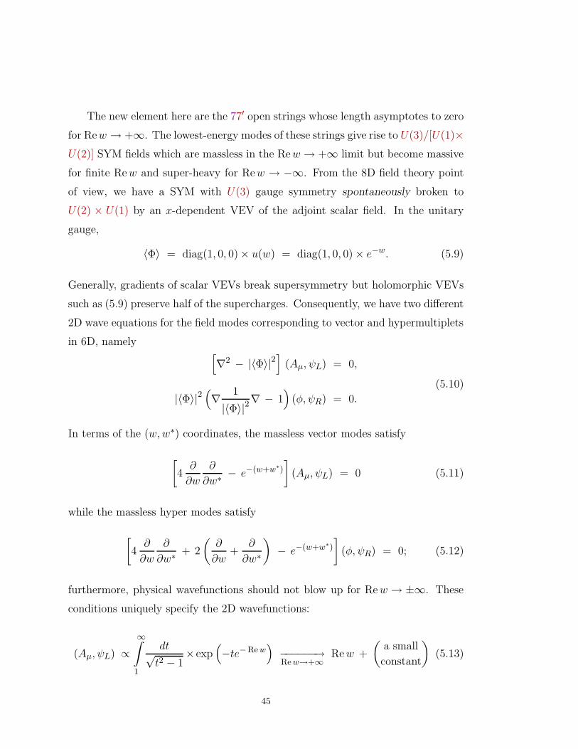
The new element here are the 77′ open strings whose length asymptotes to zero

for Rew → +∞. The lowest-energy modes of these strings give rise to U(3)/[U(1)×U(2)] SYM fields which are massless in the Rew → +∞ limit but become massive

for finite Rew and super-heavy for Rew → −∞. From the 8D field theory point

of view, we have a SYM with U(3) gauge symmetry spontaneously broken to

U(2) × U(1) by an x-dependent VEV of the adjoint scalar field. In the unitary

gauge,

〈Φ〉 = diag(1, 0, 0)× u(w) = diag(1, 0, 0)× e−w. (5.9)

Generally, gradients of scalar VEVs break supersymmetry but holomorphic VEVs

such as (5.9) preserve half of the supercharges. Consequently, we have two different

2D wave equations for the field modes corresponding to vector and hypermultiplets

in 6D, namely[

∇2 − |〈Φ〉|2]

(Aµ, ψL) = 0,

|〈Φ〉|2(

∇ 1

|〈Φ〉|2∇ − 1

)

(φ, ψR) = 0.

(5.10)

In terms of the (w,w∗) coordinates, the massless vector modes satisfy

[

4∂

∂w

∂

∂w∗− e−(w+w∗)

]

(Aµ, ψL) = 0 (5.11)

while the massless hyper modes satisfy

[

4∂

∂w

∂

∂w∗+ 2

(

∂

∂w+

∂

∂w∗

)

− e−(w+w∗)

]

(φ, ψR) = 0; (5.12)

furthermore, physical wavefunctions should not blow up for Rew → ±∞. These

conditions uniquely specify the 2D wavefunctions:

(Aµ, ψL) ∝∞∫

1

dt√t2 − 1

×exp(

−te−Re w)

−−−−−−→Re w→+∞

Rew +

(

a small

constant

)

(5.13)

45

for the massless 6D vector multiplets and

(φ, ψR) ∝∞∫

1

dt√t2 − 1

× te−Rew exp(

−te−Re w)

−−−−−−→Rew→+∞

1 (5.14)

for the massless hypermultiplets. Note that both wavefunctions describe (the zero

energy limit of) unbound motion of a particle in the semi-infinite Rew >∼ 0 region;

there are no bound states.

In T-dual terms, we have a 7D U(3) SYM living on the three D6 branes at

x6 ≥ b. At the junction, the U(3) group is abruptly broken to its U(1) × U(2)

subgroup while the remaining U(3)/[U(1) × U(2)] SYM fields satisfy reflecting

boundary conditions at x6 = b. According to eqs. (5.13) and (5.14), the bound-

ary conditions are Dirichlet for the 8–SUSY vector multiplet fields and Neumann

for the hypermultiplet fields. Furthermore, there are no massless 6D fields local-

ized at the junction. Although classically the 68 open strings have zero length at

the junction, they do not have massless modes because of world-sheet quantum

corrections. Indeed, the 68 strings are T-dual to the 7′7 strings giving rise to the

U(3)/[U(1)×U(2)] SYM fields — which have no normalizable zero modes localized

in the junction area.

The above discussion concerns the D6–D8 junction at x6 = b. There is another

junction at x6 = 0 — denoted by the yellow rectangle in fig. (5.7) — where two

D6 branes reach the O8 orientifold plane accompanied by seven D8 branes. As

explained in §4.3, at this second junction the U(2) gauge symmetry is broken to

Sp(1) = SU(2), the 3 vector multiplets satisfy Neumann boundary conditions at

x6 = 0 while the 3 hypermultiplets satisfy Dirichlet conditions and the 86 open

strings give rise to localized 6D massless particles forming half-hypermultiplets in

the (2, 14) representation of the SU(2)× SO(14) gauge group.

The two junctions at x6 = b and x6 = 0 are distinct in the type I′/D6 theory,

but in the Horava–Witten theory b→ 0 and the two junctions collapse into a single

46

I5 intersection plane. The local physics on this plane is simply the net effect of

the two junctions of the dual type I′/D6 model translated into HW orbifold terms:

1. The 7D SU(3) gauge symmetry (we discard the U(1) center of the U(3) as

explained in §4.2) is broken to SU(2)×U(1). Furthermore, the U(1) ⊂ SU(3)

and the 10D U(1) ⊂ E8 are broken to the diagonal U(1). The net gauge

symmetry on the intersection plane is therefore

G6Dlocal = SU(2)× U(1)× SO(14) (5.15)

2. The local 6D massless fields at the I5 comprise a half-hypermultiplet in the

(2, 0, 14) representation of (5.15).

3. The 7D SYM fields have boundary conditions depending on their SU(2) ×U(1) and 8–SUSY quantum numbers. Decomposing the SU(3) adjoint 8 as

(3, 0) + (1, 0) + (2,±1) and 16–SUSY vector multiplet as 8–SUSY vector +

hyper-multiplets, we have

(3, 0) vector: Neumann b.c., (3, 0) hyper: Dirichlet b.c.,

(1, 0) vector: Locking b.c., (1, 0) hyper: Neumann b.c.,

(2,±1) vector: Dirichlet b.c., (2,±1) hyper: Neumann b.c.(5.16)

Note that the boundary conditions (5.16) are rather complicated compared to

the models presented in ref. [3] — where all vector multiplets at the same boundary

had similar boundary conditions and ditto for the hypermultiplets. Furthermore,

the specific gauge symmetry breaking (5.15) following from the conditions (5.16)

is totally counter-intuitive from the heterotic point of view; indeed, the unbroken

SU(2) factor of the local symmetry (5.15) does not exist in the heterotic orbifold’s

spectrum and the twisted states’ charges (5.3) do not indicate any hidden SU(2)

symmetry either. A bit later in this section, we shall brane engineer the removal

of this unwanted SU(2) from the massless spectrum of the 6D theory, but first we

would like to show that its existence as a local symmetry at the I5 is crucial to

the local anomaly cancellations.

47

Indeed, the locally visible charged chiral fields at the intersection plane weighed

by their contributions to the local anomaly (cf. section 2) comprise

Q6 = 12(2, 0, 14),

Q7 =1

2[2(2,+1, 1)1 + (1, 0, 1) − (3, 0, 1)] ,

Q10 =1

9

[

(1,+12 , 64) + (1,−1, 14) − (1, 0, 91) − (1, 0, 1)

]

,

(5.17)

and it’s a matter of (boring) algebra to verify conditions (2.11) and (2.12) of

complete anomaly cancellation. Specifically, the magnetic charge g vanishes for

the symmetric orbifold, thus

dim(Q = Q6 +Q7 +Q10) = 0 + 1219 (5.18)

which provides for cancellation of the irreducible tr(R4) anomaly, and

A′ = 23 TrQ(F 4) − 1

6 tr(R2)× TrQ(F 2) + 118(tr(R2))2

= 0 +(

trF 2SO(14) + 2F 2

U(1) − 12 trR2

)

×(

trF 2SU(2) + 4

3F2U(1) − 1

9 trR2)

(5.19)

which lets the rest of the one-loop anomaly cancel against the inflow and intersec-

tion anomalies.⋆

It is very important that the (trF 2SU(2))

2 term cancels out of the one-loop

anomaly (5.19) because the inflow and intersection anomalies cannot possibly can-

cel un-mixed anomalies of gauge symmetries of purely 7D origins. Such cancella-

tion requires both hyper- and vector multiplets with non-trivial SU(2) quantum

numbers to be locally visible at the intersection plane — and of course the vector

multiplets are the 7D fields with Neumann boundary conditions which are respon-

sible for the SU(2)’s existence in the first place. Now suppose we did not have

the unbroken SU(2) but only its U(1) subgroup (which eventually mixes with the

U(1) ⊂ E(2)8 at the other end of x6). In such a hypothetical model, two out of 3

⋆ Actually, the inflow anomaly vanishes for this model because of g = 0.

48

vector multiplets would have Dirichlet rather than Neumann boundary condition

and the only vector multiplet visible at the intersection plane would be the gener-

ator of the U(1) — which is neutral. On the other hand, there would be plenty of

locally present U(1)–charged hypermultiplets — and we would be stuck with the

resulting F 4U(1) local anomaly we would have no way of canceling.

In other words, cancellation of the F 4U(1) local anomaly requires local pres-

ence of U(1)–charged vector multiplets — and hence embedding the U(1) into

a locally unbroken non-abelian symmetry group. For the Z3 model in question,

local anomaly cancellation favors local spectrum (5.17) and hence boundary con-

dition (5.16). Such boundary conditions are very strange from the heterotic point

of view; discovering them without the benefit of the dual type I′/D6 model would

have been rather difficult.

Our next task is therefore to brane engineer the correct twisted spectrum (5.3)

of the heterotic orbifold; in particular, we need to break the un-observed SU(2)

symmetry. In the dual type I′/D6 model, let us shift our attention from the

left terminus (5.7) of the three D6 branes to the big picture (5.6). Thanks to

E(1)8 ↔ E

(2)8 symmetry of the model, the right terminus of the D6 branes also

looks like (5.7) (modulo x6 → L− x6), but this leaves open the question whether

the D6 branes terminating on the outlier D8 branes on the left and on the right

are two ends of the same D6 brane or two distinct D6 branes. Thus we have two

distinct brane models, namely

49

0 b LL− bx6

O8

+7D

8SO

(14)

1D8

U(1

)

O8

+7D

8SO

(14)

1D8

U(1

)

3D6

SU(3)

Dual to the M91 Dual to the M92

x7,8

,9 (5.20)

and

0 b LL− bx6

O8

+7D

8SO

(14)

1D8

U(1

)

O8

+7D

8SO

(14)

1D8

U(1

)

3D6

SU(3)

Dual to the M91 Dual to the M92

x7,8

,9 (5.21)

In each model, the 7D SU(3) gauge symmetry is broken down to an SU(2)×U(1)

subgroup at both purple junctions (x6 = b and x6 = (L−b)), but there is one crucial

difference: In the first model (5.20), the two junctions preserve the same SU(2)×U(1) ⊂ SU(3) at both ends, hence the same 3 7D gauge fields have Neumann

50

boundary conditions at both ends of x6 and therefore zero modes. Consequently,

the 6D effective theory contains massless SU(2) gauge fields of purely 7D origin.

In the dual heterotic terms, this means a non-perturbative 6D SU(2) SYM at each

fixed plane of the T 4/Z3 orbifold in addition to the perturbative gauge fields in

the untwisted sector. This is a very interesting heterotic string model in its own

right, but unfortunately it is quite different from the perturbative T 4/Z3 orbifold

we started from.

By contrast, in the second model (5.21) the two purple junctions preserve two

different SU(2) × U(1) subgroups of the SU(3).⋆

Because of this mis-alignment,

the 3 vector fields with Neumann boundary conditions at x6 = b have Dirichlet

or locking boundary conditions at x6 = (L − b) and vice verse, hence no zero

modes and no purely non-perturbative vector multiplets in the twisted sector of

the heterotic orbifold. The abelian U(1) × U(1) ⊂ SU(3) vector fields which mix

with the 9D abelian fields according to eq. (5.5) belong to the overlap of the two

surviving subgroups of the SU(3) at each junction,

[SU(2)× U(1)]1 ∩ [SU(2)× U(1)]2 = U(1)× U(1). (5.22)

To keep track of the U(1) × U(1) charges of various 7D fields we need two

orthogonal commuting generators of the SU(3). The SU(3)→ [SU(2)×U(1)]1 →U(1)× U(1) chain of symmetry breaking suggests

T1 = diag(+12 ,−1

2 , 0) and Y1 = diag(+13 ,+

13 ,−2

3) (5.23)

while the SU(3)→ [SU(2)× U(1)]2 → U(1)× U(1) chain suggests

T2 = diag(0,+12 ,−1

2) and Y2 = diag(−23 ,+

13 ,+

13); (5.24)

⋆ To be precise, the two subgroups are equivalent via an SU(3) isomorphism W 6= 0. In gauge

invariant terms, W = P exp(

∫

L−b

bA6dx6

)

× a non-trivial element of the Weyl group of the

SU(3).

51

the two sets of charges are related to each other according to

T1 = −12T2 − 3

4Y2

Y1 = +T2 − 12Y2

⇔

T2 = −12T1 + 3

4Y1

Y2 = −T1 − 12Y1

. (5.25)

For completeness sake, the table below lists both sets of charges as well as boundary

conditions for the all the 7D SYM fields.

Charges Boundary Conditions

(T1, Y1) (T2, Y2) 8–SUSY vector hyper

(±1, 0) (∓12 ,∓1) (Neumann,Dirichlet) (Dirichlet,Neumann)

(±12 ,±1) (±1

2 ,∓1) (Dirichlet,Dirichlet) (Neumann,Neumann)

(∓12 ,±1) (±1, 0) (Dirichlet,Neumann) (Neumann,Dirichlet)

(0, 0) (0, 0) (locking,Neumann) (Neumann,Dirichlet)

(0, 0) (0, 0) (Neumann,locking) (Dirichlet,Neumann)

(5.26)

As promised, none of the vector multiplets have Neumann–Neumann boundary

conditions. On the other hand, two hypermultiplets with similar charges†

have

Neumann–Neumann conditions and hence zero modes. In the dual heterotic terms,

these two zero modes manifest themselves as twisted hypermultiplets charged with

respect to U(1) × U(1) (thanks to the 10D/7D abelian field mixing (5.5)) but

singlets with respect to SO(14)× SO(14). And indeed the twisted spectrum (5.3)

of the perturbative heterotic orbifold contains precisely two such singlets per fixed

point of the T 4/Z3.

Altogether, the hypermultiplets localized at x = 0 in the brane model (5.21)

comprise one 14 of the SO(14)1 at x6 = 0, one 14 of the SO(14)2 at x6 = L, and

two singlets from zero modes spanning the whole x6.

• The (14, 1) fields have abelian charges (T1 = 12 , Y1 = 0) (from 1

2(2, 0) of the

[SU(2)× U(1)]1 local symmetry at x6 = 0) and hence (T2 = −14 , Y2 = −1

2).

† For a hypermultiplet, the overall sign of all its charges is a matter of convention. Hence,two hypermultiplets with exactly opposite charges are equivalent to two hypermultipletswith identical charges.

52

• Likewise, the (1, 14) fields have abelian charges (T2 = 12 , Y2 = 0) and hence

(T1 = −14 , Y1 = +1

2).

• Finally, the two (1, 1) singlet fields have (T1 = +12 , Y1 = +1) and (T2 =

+12 , Y2 = −1).

Comparing this spectrum to the heterotic twisted spectrum (5.3) we see full agree-

ment, provided we identify the abelian U(1)× U(1) charges according to

Cheterotic1 = CHW

U(1)⊂E(1)8

+∑

fixedplanes

[

Y1 − 23T1 = 4

3T2

]

,

Cheterotic2 = CHW

U(1)⊂E(2)8

+∑

fixedplanes

[

−Y2 − 23T2 = 4

3T1

]

.(5.27)

Weirdly, the observed abelian symmetries (5.5) of the heterotic Z3 orbifold mix

the 10D abelian charge living on the left end of the world with the 7D charge that

happens to be part of an unbroken non-abelian symmetry SU(2)2 at the right end of

the world and vice verse. In section 7 we shall see similar coincidences happening for

other orbifold models; alas, we have no explanation for this phenomenon. Instead,

we have an independent confirmation of the charges (5.27) through the gauge

couplings of the model.

Specifically, the (43T2,

43T1) 7D abelian charges at each fixed plane come with

gauge couplings

1

g27D[U(1)× U(1)]

=1

g2[SU(3)]×(

tr(43T2)

2 tr((43T2)(

43T1))

tr((43T2)(

43T1)) tr(4

3T1)2

)‡

=1

g2[SU(3)]×(

169 −8

9

−89

169

)

,

(5.28)

hence the observed abelian charges (5.27) have

1

g2[U(1)× U(1)]=

2

g2[E8 ×E8]+

9

g2[SU(3)]×(

169 −8

9

−89

169

)

(5.29)

‡ Note normalization tr ≡ 2 Tr3 .

53

where the factor 9 in the second term stems from 9 fixed planes of the T 4/Z3

orbifold. (The factor 2 in the first term comes from the normalization of the

U(1) ⊂ E8 charges, 130 Tr248(CU(1)⊂E8

)2 = 2.) The two E8 couplings are equal for

the symmetric Z3 orbifold (12 instantons in each E8 hence k1 = k2 = 0), thus in

terms of the coefficients v, v in eq. (2.5) the abelian charges have

v[U(1)× U(1)] =

(

2 0

0 2

)

, v[U(1)× U(1)] =

(

16 −8

−8 16

)

. (5.30)

On the other hand, for any perturbative heterotic model in 6D, the coefficients

v, v follow from the model’s massless spectrum via factorization of the net 6D

anomaly polynomial according to eq. (2.2). Evaluating and factorizing the anomaly

polynomial for the symmetric T 4/Z3 orbifold model is a straightforward albeit

tedious exercise which eventually yields

v[SO(14)1] = v[SO(14)2] = 1, v[U(1)× U(1)] =

(

2 0

0 2

)

,

v[SO(14)1] = v[SO(14)2] = 0, v[U(1)× U(1)] =

(

16 −8

−8 16

)

,

(5.31)

in full agreement with eq. (5.30) based on the specific charges (5.27).

To summarize, we have a HW description of the symmetric T 4/Z3 heterotic

orbifold which passes all the consistency conditions, the twisted spectrum, the

gauge couplings, the local anomalies, the works. Furthermore, this description

is based on the type I′/D6 brane model (5.21) which explains all the Mysterious

phenomena at the I5 intersection planes. Indeed, the fairly straightforward logic

of brane engineering leads directly to the correct HW solution — which looks weird

but works well.

54

5.2 A Z4 Model

Our next model is a T 4/Z4 heterotic orbifold in which the first E(1)8 is broken

to SO(12)×SU(2)×U(1) (lattice shift vector δ1 = (−34 ,

14 , 0, 0, 0, 0, 0, 0)) while the

second E(2)8 is broken to SO(16) (shift vector δ2 = (1, 0, 0, 0, 0, 0, 0, 0)). In terms

of the unbroken subgroups, the α1 : Z4 7→ E(1)8 twist acts according to

α1(248) = + [(66, 1, 0) + (1, 3, 0) + (1, 1, 0)] − [(32′, 2, 0) + (1, 1,±2)]

+ i [(32, 1,+1) + (12, 2,−1)] − i [(32, 1,−1) + (12, 2,+1)].(5.32)

while the α2 : Z4 7→ E(2)8 twist acts as

α2(248 = 120 + 128) = +(120) − (128). (5.33)

Note (α2)2 = 1, hence all massless hypermultiplets in the untwisted and the doubly-

twisted sectors are singlets with respect to the SO(16) ⊂ E2)8 . Altogether, the

massless spectrum of this model comprises:

• In the untwisted sector: SUGRA+1 tensor multiplet (the dilaton); 190 vector

multiplets in the adjoint representation of the

G = [SO(12)× SU(2)× U(1)]× SO(16); (5.34)

2 moduli and 56 charged hypermultiplets,

H0 = (12, 2,+1;1) + (32, 1,−1; 1) + 2M. (5.35)

• In the singly-twisted sector: 32 charged hypermultiplets for each of the 4 Z4

fixed points on the T 4,

H1 = 4(1, 2,−12 ; 16). (5.36)

55

• In the doubly-twisted sector:

H2 = 6× 12(32, 1, 0; 1) + 10× 1

2(12, 2, 0; 1) + 32(1, 1,+1;1). (5.37)

In terms of individual O6 fixed planes, the orbifold has 6 Z2 fixed planes where

the E(1)8 is broken to [E7 ⊃ SO(12)× SU(2)]× [SU(2) ⊃ U(1)], the E

(2)8 remains

unbroken and the twisted hypermultiplets comprise 12(56, 1; 1) + 2(1, 2; 1), plus 4

Z4 fixed planes each having gauge symmetry (5.34) and twisted hypermultiplets

Htw = (1, 2,−12 ; 16) + 1

2(12, 2, 0; 1) + 2(1, 1,+1;1). (5.38)

In the HW picture, the twisted states’ charges (5.38) require the SU(2)×U(1)

gauge fields to span the x6 dimension between the end-of-the-world M9 branes

along the O6 fixed planes, thus

SU(2)× U(1)net = diag[

(SU(2)× U(1))10D ×∏

Z4 fixedplanes

(SU(2)× U(1))7D

]

.

(5.39)

(The 7D gauge fields on the Z2 fixed planes do not participate in this mixing, cf.

discussion of the [E7 × SU(2)] × E(2)8 model in ref. [3].) The actual 7D gauge

symmetry on a Z4 fixed plane is of course SU(4); somehow, we need to break it

down to a non-maximal SU(2) × U(1) subgroup, then impose locking boundary

conditions on the 7/10 D SU(2)× U(1) fields at the I51 intersection.

Again, the solution comes courtesy of the dual type I′/D6 brane model:

56

0 b Lx6

O8

+6D

8

SO

(12)

2D8

U(2

)

O8

+8D

8SO

(16)

4 D6

SU(4)

Dual to the M91 Dual to the M92

x7,8

,9 (5.40)

At the right terminus of the four coincident D6 branes dual to a Z4 fixed plane, all

four D6 branes end on the O8 orientifold at x6 = L. Junctions of this type were

discussed in §4.3, so let us simply quote the results for the case at hand (N = 4,

k = 8):

• The SU(4) gauge symmetry on the D6 world volume is broken at x6 = L

down to Sp(2) ⊂ SU(4).

• The 7D SYM fields form the adjoint 15 representation of SU(4). In terms

of the Sp(2) ⊂ SU(4), 15 = 10( ) + 5(˜) and the boundary conditions for

the corresponding fields are as follows:

10 vector: Neumann, 10 hyper: Dirichlet,

5 vector: Dirichlet, 5 hyper: Neumann.(5.41)

• The 68 open strings produce 6D hypermultiplets localized at the junction.

Their Sp(2)× SO(16) quantum numbers are

6DH = 12(4, 16). (5.42)

Almost at the other end of the world, at x6 = b we have two of the D6 branes

terminating at the two outlier D8 branes while the other two D6 branes continue

57

toward the orientifold plane at x6 = 0. For the sake of SU(2)9D × SU(2)7D →SU(2)diag gauge symmetry mixing we let each of the first two D6 branes terminate

on a separate D8. Altogether, the junction at x6 = b is T-dual to

2 D7′

U(2)2

2 D7

U(2)1

→ U(4) (5.43)

in the same manner as a similar junction in §5.1 is T-dual to (5.8). The physical

consequences are also similar: There is a U(2)1 SYM living on the two curved D7

branes, another U(2)2 SYM living on the two flat D7′ branes, plus U(4)/[U(2)1 ×U(2)2] SYM fields which are asymptotically massless for x6 ≫ b but become heavy

and decouple for x6 <∼ b. It T-dual terms, we have a 7D SYM whose U(4) gauge

symmetry (at x6 ≥ b) is abruptly broken down to U(2)1 × U(2)2 by boundary

conditions at x6 = b. Specifically, the coset U(4)/[U(2)1 × U(2)2] SYM fields

satisfy Dirichlet boundary conditions for the 8–SUSY vector multiplet components

and Neumann for the hypermultiplet components. Also, in spite of zero length of

the 68 open strings at the junction, there are no 6D massless fields localized at

x6 = b. Furthermore, the U(2)1 vector fields satisfy locking boundary conditions

which break U(2)7D1 ×U(2)9D → U(2)diag while the corresponding hypermultiplets

satisfy Neumann boundary conditions.

On the other hand, the U(2)2 SYM fields do not have any boundary conditions

at x6 = b and continue unmolested toward the ultimate boundary at x6 = 0. The

physics at this boundary follows from two D6 branes terminating on an O8 orien-

tifold plane, cf. §4.3: The U(2) gauge symmetry is broken to Sp(1) = SU(2), the

3 vector multiplets satisfy Neumann boundary conditions while the 3 hypermul-

tiplets satisfy Dirichlet condition, and the 68 open strings give rise to a localized

58

6D massless half-hypermultiplet in the (2, 12) representation of the locally visible

SU(2)× SO(12) gauge group.

In the HW picture of the type I′/D6 model (5.40), the two separate brane

junctions at x6 = 0 and x6 = b collapse into a single I51 intersections plane. The

local physics at this plane is simply the net effect of the two junctions, modulo

decoupling of the U(1) center of the 7D U(4) SYM related to the center-of-mass

motion of the four D6 branes. Thus:

1. The 7D gauge symmetry SU(4) is broken down to SU(2)1 × U(1)× SU(2)2

and furthermore, the [SU(2)1×U(1)] ⊂ SU(4) and the 10D [SU(2)×U(1)] ⊂E

(1)8 are broken to the diagonal SU(2)× U(1). The net gauge symmetry at

the I51 is therefore

G6Dlocal = SO(12)10D × [SU(2)1 × U(1)]diag × SU(2)2

7D. (5.44)

2. The boundary conditions for the 7D SYM fields depend on their SU(2)1 ×U(1)×SU(2)2 as well as 8–SUSY quantum numbers. Decomposing the SU(4)

adjoint 15 as (3, 0, 1) + (1, 0, 3) + (1, 0, 1) + (2,±1, 2), we have

(3, 0, 1) vector: Locking b.c., (3, 0, 1) hyper: Neumann b.c.,

(1, 0, 1) vector: Locking b.c., (1, 0, 1) hyper: Neumann b.c.,

(1, 0, 3) vector: Neumann b.c., (1, 0, 3) hyper: Dirichlet b.c.,

(2,±1, 2) vector: Dirichlet b.c., (2,±1, 2) hyper: Neumann b.c.(5.45)

3. The local 6D massless fields at the intersection comprise a half-hypermultiplet

in the (12, 1, 0, 2) representation of (5.44).

Note that the heterotic twisted spectrum (5.38) contains a similar (12, 2, 0)

half-hypermultiplet, but the (12, 1, 0, 2) particles we see at the I51 intersection are

doublets of the wrong SU(2)! Hence, for duality’s sake, we must somehow mix this

purely 7D SU(2)2 with the already mixed SU(2)1 = diag(

SU(2)7D1 × SU(2)10D)

.

This second diagonalization occurs not at the I51 but at the I52 at the other

59

end of the world: the SU(4) → Sp(2) breaking locks the two 7D SU(2)1,2 gauge

symmetries together. To see how this works, consider the net result of the SU(4)

breaking at both ends of the O6,

SU(4) −→ SU(2)1 × SU(2)2 × U(1)

↓ ↓Sp(2) −→ ??

(5.46)

To clarify this diagram, we identify

SU(4) = SO(6), Sp(2) = SO(5), SU(2)×SU(2)×U(1) = SO(4)×SO(2),

(5.47)

and note two distinct options for the overlap

SO(5) ∩ [SO(4)× SO(2)] =

SO(3)× SO(2) = SU(2)× U(1)

or SO(4) = SU(2)× SU(2).(5.48)

Because the U(1) is observed in the heterotic theory, we choose the first option

and consequently

SU(4) −→ SU(2)1 × SU(2)2 × U(1),

↓ ↓Sp(2) −→ SU(2)1+2 × U(1)

(5.49)

where SU(2)1+2 = diag (SU(2)1 × SU(2)2) (cf. SO(3) ⊂ SO(4)).

Ultimately, the SU(2) observed in the heterotic theory is the common diagonal

of the

SU(2)10D ×∏

Z4 fixedplanes

[SU(2)1 × SU(2)2]7D. (5.50)

At each O6[Z4] fixed plane of the HW picture, the SU(2) quantum numbers of the

60

12(12, 2) twisted hypermultiplet follow a weird trajectory

12(12, 1, 0, 2) SU(2)2 ⊂ SU(4)7D

SU(2)1 ⊂ SU(4)7D

SU

(2)⊂E

(1)

812(12, 2, 0; 1)

(5.51)

from the x6 = 0 end of the fixed plane all the way to the other end x6 = L and

back to x6 = b ≈ 0. At the end of this trajectory, the 12(12, 1, 0, 2) multiplet of the

local gauge symmetry (5.44) indeed becomes the 12(12, 2, 0; 1) multiplet of the net

6D gauge symmetry (5.34). We admit however that such a HW origin of a twisted

state’s quantum numbers is so bizarre, we would have never found it without the

dual type I′/D6 model (5.40).

The HW origins of the remaining twisted states (5.38) are less complicated.

The 12(4, 16) multiplet of the Sp(2)× SO(16) living at I52 at the right end of the

fixed plane becomes (1, 2,+12 ; 16) of the net 6D symmetry (5.34) after the SP (2) is

broken down to SU(2)×U(1) which eventually mixes with the 10D SU(2)×U(1)

at x6 = b ≈ 0. Indeed, in SO(5) terms, the 4 representation of the Sp(2) is

the spinor, hence it decomposes as 4 = (2,+12) + (2,−1

2) with respect to the

SO(3)× SO(2) ⊂ SO(5); therefore, for a hypermultiplet 12(4) = (2,+1

2).

Finally, the two charged singlets in the twisted spectrum (5.38) arise from the

zero modes of the 7D fields. Indeed, let us arrange the 15 7D SYM fields according

to their SU(2)1+2 × U(1) quantum numbers and note their boundary conditions

61

at both ends of the x6:

Charges Boundary Conditions

SU(2)1+2 × U(1) 8–SUSY vector hyper(

3, 0)

(locking,Neumann) (Neumann,Dirichlet)(

1, 0)

(locking,Neumann) (Neumann,Dirichlet)(

3, 0)

(Neumann,Dirichlet) (Dirichlet,Neumann)(

3, ± 1)

(Dirichlet,Neumann) (Neumann,Dirichlet)(

1, ± 1)

(Dirichlet,Dirichlet) (Neumann,Neumann)

(5.52)

According to this table, two hypermultiplets on the last line have Neumann bound-

ary conditions at both ends and hence massless (in 6D) zero modes. The (1,±1)

charges of these hypermultiplets are exactly opposite and therefore equivalent; in

the (5.34) terms, we have 2(1, 1,+1, 1), cf. the last entry in the heterotic twisted

spectrum (5.38).

To summarize the above discussion, the HW dual of the type I′/D6 brane

model (5.40) correctly reproduces the twisted spectrum of the heterotic Z4 fixed

plane, albeit in a rather weird manner. To justify this weirdness, we conclude

this section by verifying the other kinematical requirements of the HW orbifold,

namely the heterotic gauge couplings and the local anomaly cancelation at both

I51,2 intersection planes.

We begin with the gauge couplings: According to eq. (5.50), the net SU(2)

gauge theory of the orbifold involves two copies of the SU(2) embedded in the

SU(4) at each Z4 fixed plane. Consequently,

1

g2[SU(2)]=

1

g2[E(1)8 ]

+4× 2

g2[SU(4)](5.53)

or in terms of the v, v coefficients,

v[SU(2)] = 1, v[SU(2)] = 12k1 + 8. (5.54)

The generator C7D of the U(1) ⊂ SU(4) has eigenvalues (+12 ,+

12 ,−1

2 ,−12) hence

the norm tr(C27D) = 2 while the generator C10D of the U(1) ⊂ E

(1)8 is normalized

62

to tr(C210D) = 4, thus the net U(1) of the orbifold has

v[U(1)] = 4, v[U(1)] = 2k1 + 4× 2. (5.55)

Finally, the remaining SO(12) and SO(16) gauge factors are of purely 10D origins,

therefore

v[SO(12)] = v[SO(16)] = 1, v[SO(12)] = 12k1 , v[SO(16)] = 1

2k2 .

(5.56)

Formulæ (5.54) through (5.56) are predictions of the HW picture of the orb-

ifold which is itself a prediction of the type I′/D6 dual model (5.40). To verify

these predictions, we calculated the net anomaly polynomial of the orbifold and

factorized it according to eq. (2.2). After some boring arithmetic, we arrived at

v[SO(12)] = 1, v[SO(12)] = +2,

v[SU(2)] = 1, v[SU(2)] = +10,

v[U(1)] = 4, v[U(1)] = +16,

v[SO(16)] = 1, v[SO(16)] = −2,

(5.57)

which indeed agrees with eqs. (5.54), (5.55) and (5.56) for k1 = +4, k2 = −4 (i.e.,

16 instantons in the E(1)8 and 8 in the E

(2)8 ).

Next, consider the local anomalies at the I51 intersection plane where the local

gauge symmetry is given by eq. (5.44). The anomaly-weighed chiral spectrum at

this plane comprises

Q6 = 12(12, 1, 0, 2),

Q7 =1

2

[

(1, 3, 0, 1) + (1, 1, 0, 1) − (1, 1, 0, 3) + (1, 2,±1, 2)]

,

Q10 =1

32

[

(12, 2,±1, 1) + (32, 1,±1, 1)]

+3

32

[

(32′, 2, 0, 1) + (1, 1,±2, 1)]

− 5

32

[

(66, 1, 0, 1) + (1, 3, 0, 1) + (1, 1, 0, 1)]

,

(5.58)

63

while the plane’s magnetic charge is

g1[Z4] =1

4

(

k1 − 6g1[Z2])

=1

4

(

4 − 6× 3

4

)

= −1

8, (5.59)

thus we can easily verify that

dim(Q = Q6 +Q7 +Q10) =61

4= 19 + 30× −1

8(5.60)

and hence the tr(R4) anomaly cancels out, cf. eq. (2.11). The rest of the anomaly

follows via straightforward if tedious evaluation of

A′ ≡ 23 TrQ(F4) − 1

6 tr(R2)× TrQ(F2) + (18g + 1

2T (1) = 116)(

tr(R2))2

=−1

16

(

tr(F 2SO(12)) + tr(F 2

SU(2)) + 4F 2U(1) − 1

2 tr(R2))2

+(

tr(F 2SO(12)) + tr(F 2

SU(2)1) + 4F 2

U(1) − 12 tr(R2)

)

×(

tr(F 2SU(2)1

) + 2F 2U(1) + tr(F 2

SU(2)2) − 5

32 tr(R2))

,

(5.61)

which indeed shows cancellation of the one-loop anomaly against the inflow and

intersection anomalies, cf. eq. (2.12).

The SU(2) trajectory (5.51) goes through the I51 intersection twice, hence two

separate SU(2) gauge factors in the local symmetry (5.44). To see the importance

of this setup anomaly-wise, suppose we had only one SU(2)1+2 factor instead and

focus on the(

tr(F 2SU(2))

)2anomaly term. In the SU(2)1+2 terms, the 15 7D SYM

fields comprise four triplets and three singlets, and in our hypothetical model all the

triplets would have to have Dirichlet or locking boundary conditions for the vector

fields in order to prevent the appearance of a second SU(2) factor. Anomaly-wise,

the effect of this change is to change the sign of the third term in eq. (5.58) for the

Q7 from negative to positive — and therefore to increase the one-loop TrQ(F 4SU(2))

by +2(

tr(F 2SU(2))

)2. At the same time, the Q6, the Q10 and all the terms in the

inflow and intersection anomalies are completely fixed by the heterotic data, so

64

they must remain unchanged. Altogether, we would have +2(

tr(F 2SU(2))

)2worth

of un-canceled local anomaly — which rules out the single SU(2) hypothesis. On

the other hand, the setup with two local SU(2) gauge symmetries leads to complete

anomaly cancellation. Thus, the trajectory (5.51) may look weird, but it works

and nothing else seem to do the job, so it must be right!

Finally, at the I52 intersection plane, the local gauge symmetry is SO(16)×Sp(2), the anomaly-weighed chiral spectrum comprises

Q6 = 12(16, 4),

Q7 =1

2

[

(1, 5) − (1, 10)]

,

Q10 =3

32(128, 1) − 5

32(120, 1),

(5.62)

and the magnetic charge is g2 = −g1 = +18 . We immediately see that eq. (2.11) is

satisfied,

dim(Q = Q6 +Q7 +Q10) =91

4= 19 + 30× +1

8, (5.63)

and after a bit of arithmetic we can see that eq. (2.12) is satisfied as well,

A′ ≡ 23 TrQ(F4) − 1

6 tr(R2)× TrQ(F2) + (18g + 1

2T (1) = 332)(

tr(R2))2

=+1

16

(

tr(F 2SO(16)) − 1

2 tr(R2))2

+(

tr(F 2SO(12)) − 1

2 tr(R2))

×(

tr(F 2Sp(4)) − 5

32 tr(R2))

.

(5.64)

Again, cancelation of the net tr(F47D) anomaly does not allow any changes in Q7

(since all the other contributions to this anomaly are fixed by the heterotic data),

which confirms that the 7D vector fields with Neumann boundary conditions should

indeed comprise the adjoint 10 multiplet of the Sp(2) ⊃ SU(2)×U(1), exactly as

in the dual type I′/D6 brane model.

65

6. NS5 Half–Branes at the End of the World

In this section, we add another tool to our brane engineering toolkit, namely

NS5 branes serving as terminals of several coincident D6 branes. Or rather NS5

half-branes, stuck on the O8 orientifold planes and unable to move in the x6 direc-

tion. Such half-branes are explained in some detail in refs. [11,30]; the following

couple of pages give a brief summary of relevant phenomena.

An NS5 half-brane terminus of N D6 branes results from O8 orientifold pro-

jection of the following picture:

N D6

U(N)1

N D6

U(N)2

NS5 (6.1)

In the middle of this picture we have an NS5 brane — a supersymmetric co-

dimension 4 soliton of the metric, dilaton and Bµν fields of the type IIA superstring.

The metric is asymptotically flat for r →∞ but develops an infinite S3×R+ throat

at r → 0; deep down the throat, the string coupling λ = eϕ increases and eventually

becomes strong. The D6 branes approaching the NS5 brane from the right (i.e.,

x = 0, x6 → +0) plunge down the throat and eventually suffer some kind of a

‘meltdown’ in the strong coupling region. In the local metric (string frame), the

x6 → +0 dimension of these D6 branes is infinite and there is no terminus, but the

continuously rising string coupling causes reflection of the 7D particles living on the

D6 world-volume back to x6 → +∞. Hence, from the low-energy / long-distance

point of view, the 6D branes appear to terminate on the NS5 brane where the 7D

U(N) SYM fields have reflecting boundary conditions: Neumann for the 8–SUSY

vector multiplet components and Dirichlet for the hypermultiplet components.

66

On the left side of the picture (6.1) we have N more D6 branes at x6 < 0;

they also plunge down the NS5 throat for x6 → −0, but the two sets of D6 branes

remain at finite distance from each other all the way down. Therefore, the U(N)

SYM fields at x6 < 0 suffer reflecting boundary conditions at x6 = −0 without any

locking onto the similar SYM fields at x6 = +0, hence locally at x6 = 0 we have a

double gauge symmetry U(N)L×U(N)R. Or rather SU(N)L×SU(N)R×U(1)L−R

whereas the other U(1)L+R is Higgsed out by quantum corrections (the Fayet–

Iliopoulos term and its superpartners); the hypermultiplet ‘eaten up’ by this Higgs

effect corresponds to moving the NS5 brane in the x7,8,9,10 directions separately

from the D6 branes. On the other hand, moving the NS5 brane in the x6 direction

corresponds to the scalar in the 8–SUSY tensor multiplet, which remains in the

massless spectrum of the configuration.

Finally, we have open strings connecting the two sets of the D6 branes in the

throat region. Such strings have short O(√α′) but non-zero length; nevertheless

they have zero modes giving rise to 6D massless hypermultiplets localized at x6 = 0.

Naturally, the gauge quantum numbers of these particles are (N,N).

The O8 orientifold projection identifies the two halves of the picture (6.1)

as mirror images of each other: The physical part of the NS5 brane is only a

half-brane and there is only one independent set of N D6 branes. The 7D SYM

fields surviving the projection comprise the diagonal SU(N)L+R while the U(1)

fields are projected out altogether. The tensor multiplet is also projected out;

consequently, the NS5 half-brane cannot move in the x6 direction any longer and

remains forever stuck at the orientifold plane. Finally, the (N,N) multiplet of

localized 6D fields splits into a symmetric and an antisymmetric multiplets

of the diagonal SU(N) gauge symmetry. The two multiplets have opposite signs

with respect to the orientifold projection Ω: The is Ω–negative while the is

Ω–positive, thus only the antisymmetric multiplet survives the projection.

Ultimately, from the low-energy, x6 > 0 point of view, the NS5 half-brane

serves as a new kind of a terminal junction between the D6 branes and the O8

67

orientifold plane,

Glocal = SU(N),

7DV = Adj.,

7DH = 0,

7DH = ,

12 NS5

N D6

SU(N)(6.2)

Unlike the junctions discussed in §4.3 (cf. fig. (4.6)), the 12NS5 junction (6.2) pro-

vides Neumann boundary conditions at x6 = 0 for all the 7D SU(N) 8–SUSY

vector multiplets while all the 7D hypermultiplets satisfy Dirichlet conditions.⋆

Consequently, the entire SU(N) symmetry is visible at the junction and it is no

longer necessary for the number N of the D6 branes to be even. Finally, the 12NS5

junction supports localized 6D massless hypermultiplets which form an antisym-

metric tensor representation of the SU(N). From the brane engineering point of

view, such hypermultiplets are characteristic of of NS5 half-branes and do not

occur at other types of brane junctions.

As an example of a 12NS5 junction in a type I′/D6 brane dual of a perturbative

heterotic orbifold, consider a T 4/Z6 model in which E(1)8 is broken down to SU(6)×

E3 ≡ SU(6) × SU(3) × SU(2) and E(2)8 down to SU(8) × U(1). In terms of the

lattice shift vectors, δ1 = (−56 ,

16 , . . . ,

16 , 0, 0) and δ2 = (−11

12 ,+112 , . . . ,

+112 ); in terms

of the unbroken subgroups, the α1 : Z6 7→ E(1)8 twist acts as

α1(248) = + [(35, 1, 1) + (1, 8, 1) + (1, 1, 3)] − (20, 1, 2)

+ e2πi/6(6, 3, 2) + e−2πi/6(6, 3, 2)

+ e4πi/6(15, 3, 1) + e−4πi/6(15, 3, 1)

(6.3)

⋆ As usual, we disregard the U(1) factor of the 7D U(N) as irrelevant to the orbifold problem.

68

while the α2 : Z6 7→ E(2)8 twist acts according to

α2(248) = + [(63, 0) + (1, 0)] − (70, 0)

+ e2πi/6[(28,−1) + (1,+2)] + e−2πi/6[(28,+1) + (1,−2)]

+ e4πi/6(28,+1) + e−4πi/6(28,−1).

(6.4)

In the untwisted sector of the orbifold, massless particles comprise the usual

SUGRA and dilaton multiplets, 110 vector multiplets in the adjoint of

G = [SU(6)× SU(3)× SU(2)] × [SU(8)× U(1)], (6.5)

two moduli and 65 charged hypermultiplets,

Huntw = (6, 3, 2; 1, 0) + (1, 1, 1; 1,+2) + (1, 1, 1; 28,−1) + 2M. (6.6)

The twisted sectors contain further 287 charged massless hypermultiplets; arrang-

ing them according to specific fixed O5 planes of the model (i.e., fixed points of

the T 4/Z6), we have:

• One Z6 fixed plane carries 63 hypermultiplets,

Htw[Z6] = (6, 1, 1; 8,+16) + (15, 1, 1; 1,−2

3). (6.7)

• Five Z2 fixed planes, each carrying 16 hypermultiplets,

Htw[Z2] = (1, 1, 2; 8,−12) ≡ 1

2(1, 2; 16). (6.8)

The second expression on the right hand side shows the quantum numbers of

these hypermultiplets with respect to the locally surviving gauge symmetry

GZ2= [E7×SU(2)]×SO(16). Note that each of these Z2 fixed planes works

exactly like the fixed planes of the T 2/Z2 orbifold of section 4.

69

• Four Z3 fixed planes, each carrying 36 hypermultiplets,

Htw[Z3] = (15, 1, 1; 1,−23) + (6, 1, 2; 1,−2

3)

+ 2(1, 3, 1; 1,−23) + (1, 3, 1; 1,+4

3)

≡ (27, 1; 1,−23) + 2(1, 3; 1,−2

3) + (1, 3; 1,+43).

(6.9)

Again, the second expression on the RHS indicates the representation of the

locally surviving symmetry GZ3= [E6 × SU(3)] × [E7 × U(1)]. Naturally,

there is a T 4/Z3 model with similar fixed planes, but for technical reasons

we do not discuss this model in the present article; hopefully, we shall return

to it in a future publication.

For our present purposes, we are interested in the HW point of view of the

Z6 fixed plane. In 7D, this O6 plane carries an SU(6) SYM, and it is clear from

the twisted spectrum (6.7) that the entire SU(6) gauge group is involved in com-

municating quantum numbers between the two M9 branes. That is, at the I51

intersection at x6 = 0, all the 7D SU(6) vector fields lock onto the 10D SU(6)

vector fields according to eq. (1.2) and all 35 hypermultiplet components have

Neumann boundary conditions. All the massless twisted states (6.7) are local-

ized at the other intersection I52 at x6 = L where the 7D vector multiplets have

Neumann BC and hypermultiplets Dirichlet BC. Thus,

I51

Glocal = SU(6)diag × [SU(3)× SU(2)]10D,

7DH = 35,

7DV = 0,

6DH = 0;

(6.10)

I52

Glocal = SU(6)7D × [SU(8)× U(1)]10D,

7DH = 0,

7DV = 35,

6DH = (6; 8,+16) + (15; 1,−2

3).

(6.11)

70

Clearly, this HW picture does lead to the correct twisted spectrum, and in the

Appendix we shall verify the rest of the kinematical constraints (the 6D gauge

couplings and the local anomaly cancelation at both I51 and I52 intersections),

but for now let us focus on brane engineering a dual model.

Brane-wise, two features of the I52 intersection are particularly noteworthy:

First, all of the 35 7D vector fields have Neumann boundary conditions at the I52

which preserves the entire SU(6) gauge symmetry. Second, the massless hypermul-

tiplets localized at the I52 include an antisymmetric tensor representation = 15

of this 7D symmetry. Both features cry out for an NS5 half-brane being present

at the junction dual to the I52, so let us engineer the following model:

x60 a L− b L

O8

+2D

8

E3

λ=∞

6D

8SU

(6)

8D

8U

(8)

O8

6D6

SU(6)

Dual to the M91 Dual to the M92

x7,8

,9 (6.12)

On the left side of this diagram, the distance a between the orientifold and

the outlier D8 branes is critical, hence λ = ∞ at x6 = 0 and the enhancement

of the perturbative 9D gauge symmetry from SO(4) × U(6) to E3 × SU(6). On

the right side, the distance b is less then critical, hence finite λ(x6 = L) and

the 9D gauge symmetry remains U(8) = SU(8) × U(1). The O6 fixed plane

is dual to six coincident D6 branes and the I51 intersection is dual to the D6

branes terminating on the six outlier D8 branes at x6 = a without reaching the

71

strongly coupled orientifold plane. As explained in §4.4, junctions of this type

impose locking boundary conditions (4.9) upon the appropriate gauge fields —

in the present case SU(6)7D × SU(6)10D → SU(6)diag — without giving rise to

any localized massless 6D particles. Also, the E3 = SU(2) × SU(3) gauge fields

living at x6 = 0 6= a remain mere spectators at the intersection. In other words,

our brane model (6.12) correctly explains all the Mysteries of the I51 intersection,

cf. eqs. (6.10).

The I52 intersection plane is dual to a combination of two distinct brane

junctions on the right side of the diagram (6.12). First, at x6 = L − b all six D6

branes cross eight D8 branes without terminating. At this ‘junction’ we have zero

length 68 open strings which give rise to localized massless 6D hypermultiplets in

the (6, 8) representation of the SU(6)7D × SU(8)9D gauge symmetry. Naturally,

the 7D SYM fields suffer no boundary conditions at x6 = L − b and continue

unmolested towards the second junction at x6 = L where the D6 branes meet the

NS5 half-brane. As we saw earlier in this section, the NS5 half-brane preserves

the entire SU(6)7D gauge symmetry by effectively imposing Neumann boundary

condition for all 7D vector fields and their 8–SUSY fermionic partners. At the same

time, all 7D hypermultiplets suffer Dirichlet boundary conditions while the open

strings deep in the NS5 half-brane’s throat give rise to localized hypermultiplets

in the = 15 of the SU(6).

Together, the two junctions at x6 = L and at x6 = L − b correctly reproduce

all the localized twisted states and the boundary conditions of the I52 intersection

plane of the HW picture, cf. eqs. (6.11). One Mystery however remains unex-

plained, namely the U(1) charge of the (15, 1,−23) twisted states. Naively, the

9D U(1) charge is a part of the U(8) symmetry living on the D8 world-volume at

x6 = L − b and hence should not attach to particles originating elsewhere in x6.

Since the 15 twisted states live on the NS5 half-brane at x6 = L 6= (L − b), they

should therefore remain U(1)–neutral.

Clearly, this reasoning is too naive to be true, and indeed the abelian charges

72

in the type I′ superstring theory are known to mix with each other thanks to the

x6–dependent ‘cosmological constant’[31,19] and its superpartners. Besides the

U(1) center of the U(8) on the D8 world-volume, we also have the RR one-form

of the type I′ theory and the BNS6,µ field (which is a one-form from the 9D point of

view). Both of these vector fields live in the ‘bulk’ of the type I′ theory, which puts

them in touch with the NS5 half-brane. Although we do not quite understand the

behavior of these fields in the throat region of the half-brane, it stands to reason

they might do something interesting enough to couple to the 15 twisted states

living there. Consequently, the 15 twisted states acquire an abelian charge which

we then need to identify as belonging to the U(1) ⊂ E(2)8 .

To back up this bit of wishful thinking with a mathematical argument, let

us consider the brane model (6.12) from a six-dimensional point of view. Taking

the x7,8,9 coordinates to be genuinely non-compact, we turn off the 9D gauge

couplings — which makes the corresponding symmetries global rather than local.

The symmetries originating from finite stretches of D6 branes keep finite 6D gauge

couplings and hence remain local — provided of course that they do not lock onto

global symmetries of 9D origins. Since we are now interested in the Mysteries at

the right side of the diagram (6.12) rather than the locking happening at the left

side, let us replace the whole left side with some kind of a D6 terminal which does

not break or lock the SU(6) symmetry, e.g., a free-floating NS5 brane. In other

words, consider the following model:

73

8D

8

O8

6D6

SU(6)

(6.13)

From the 6D point of view, this new model describes an SU(6) gauge theory

coupled to hypermultiplets in the (15) + 8(6) representation of the gauge group.⋆

Classically, the flavor symmetry of this model is U(1)15 × U(8)6 = U(1)× U(1)×SU(8), but in the quantum theory one combination of the abelian flavor symmetries

is destroyed by the color anomaly. The surviving anomaly-free combination is

determined by the cubic index of the color group,

Tr8(6)(F3) = 8 Tr(6)(F

3) = 4 Tr(15)(F3), (6.14)

hence the charge of the 15 hypermultiplet should be exactly −4 times the charge

of the 6. In other words, we have

G = SU(6)color × [SU(8)× U(1)]flavor,

H = (6; 8,+1) + (15; 1,−4),(6.15)

modulo an overall rescaling of the abelian charge.

⋆ There is also a tensor multiplet arising from the freely floating NS5 brane, but it’s existencedoes not affect the following argument.

74

When this picture is translated back into the type I′ language, the flavor sym-

metry SU(8)× U(1) becomes a 9D gauge symmetry which we would like to iden-

tify as the SU(8) × U(1) ⊂ E(1)8 . Consequently, the quantum numbers of the

twisted states localized at the junctions dual to the HW I52 should be exactly as

in eq. (6.15) — and indeed these are precisely the quantum numbers of the twisted

states in eq. (6.11) (modulo rescaling of the abelian charge by a factor 16).

The bottom line of this exercise is to show that the brane model does somehow

provides the 15 twisted states with a correct U(1) charge. Unfortunately, the

provenance of this charge from the type I′ point of view remains an unsolved

Mystery.

7. Junctions at Infinite String Coupling

The NS5 half-branes have strong string coupling regions hiding deep in their

throats. Other brane models have λ→∞ divergence at the O8 orientifold planes,

in full view of the 9D gauge symmetry — and in fact instrumental for brane

engineering this symmetry in the first place. In this section, we consider brane

models where such λ = ∞ orientifold planes are in direct contact with the D6

branes dual to fixed planes of the HW orbifolds.

Unfortunately, our knowledge of string theory is insufficient to directly describe

the physics of such strong-coupling brane junctions. Instead, we put the HW↔ I′

duality machinery in reverse gear and use the HW data to predict what should

happen at the λ =∞ junctions and leave the question of how it actually happens

for future research. Specifically, we consider two junction types, one involving a

λ = ∞ O8− plane of D-brane charge −8 and the other an O8∗ plane [13] of

charge −9. To keep our predictions reliable, we develop each junction using a

simple orbifold model with a clear HW picture described in our previous paper

[3], then confirm the results using a much more complicated model with the same

junction.

75

7.1 A Z4 Model with E1 Extended Symmetry.

We begin with the Z4 orbifold model of ref. [3] where the E(1)8 is broken to

E5 × SU(4) and the E(2)8 to E1 × SU(8). Conventionally, the E5 symmetry is

better known as the SO(10) and the E1 as the SU(2), but here we use the En

notation to highlight the origin of these two gauge groups in the type I′ picture of

the model:

x60 a1 L− a2 L

O8

+4D

8

E5

λ=∞

4D

8SU

(4)

8D

8SU

(8)

O8

λ=∞

E1

Dual to the M91 Dual to the M92

(7.1)

On both sides of this diagram, the outlier D8 branes are at critical distances from

the O8 planes, hence divergent λ→∞ both at x6 = 0 and at x6 = L and therefore

enhancement of the 9D gauge symmetry SO(8)× U(4)→ E5 × SU(4) on the left

side and SO(0)× U(8)→ E1 × SU(8) on the right side.

In the HW picture of this model (cf. section 2), each Z4 fixed plane of the

orbifold carries an SU(4) which locks upon the 10D SU(4) at the left intersec-

tion I51. At the right intersection I52, the SU(4)7D gauge fields have free (Neu-

mann) boundary conditions, and that’s where the twisted states live. Altogether,

76

we have

I51

Glocal = SU(4)diag × [SO(10)]10D,

7DH = 15,

7DV = 0,

6DH = 0;

(7.2)

I52

Glocal = SU(4)7D × [SU(8)× SU(2)]10D,

7DH = 0,

7DV = 15,

6DH = (4; 8, 1) + 12(6; 1, 2).

(7.3)

In brane engineering, the I51 intersection is obviously dual to a junction where

the four D6 branes (dual to the O6) terminate on the four outlier D8 branes at

x6 = a1, cf. §4.4. Engineering the I52 intersection is less obvious, but the fact that

both the (4; 8, 1) and the 12(6; 1, 2) twisted states live there evidently requires the

D6 branes to cross the eight outlier D8 branes at x6 = L − a2, reach all the way

to the λ =∞ orientifold plane at x6 = L and terminate there somehow. Thus,

x60 a1 L− a2 L

O8

+4D

8

E5

λ=∞

4D

8SU

(4)

8D

8SU

(8)

O8

λ=∞

E1

4D6

SU(4)?

Dual to the M91 Dual to the M92

x7,8

,9 (7.4)

77

the I52 splits into a simple D6–D8 brane crossing at x6 = L− a2 — which clearly

gives rise to the (4; 8, 1) twisted hypermultiplets but does nothing to the 7D SYM

fields themselves — plus a mysterious λ =∞ terminus which is supposed to fulfill

the rest of eqs. (7.3). In other words, for the sake of the HW ↔ I′ duality, we

need this terminus to produce: (1) Neumann boundary conditions for all 15 7D

vector fields, (2) Dirichlet boundary conditions for all 7D hypermultiplets, and

(3) localized 6D massless half-hypermultiplets in the (6, 2) representations of the

SU(4)× SU(2),

O8

@λ

=∞

E1

=SU

(2)

4D6

SU(4)?

Glocal = SU(4)× SU(2),

7DV = 15,

7DH = 0,

6DH = 12(6, 2).

(7.5)

Although we do not have a complete theory of this junction, we do have a

conjecture based on a ‘detuned’ version of the model. That is, in the multi–Taub–

NUT picture of the HW O6 fixed plane, let us detune the Wilson line from a Z4

twist breaking E(2)8 → SU(8) × SU(2) to a more generic U(1) twist which com-

mutes with the SU(8) subgroup but not with the SU(2). Please note that while

such a detuning breaks the duality with the T 4/Z4 heterotic orbifold model, it is a

perfectly legitimate deformation of the multi–Taub–NUT configuration of the HW

theory in its own right. In the type I′ language, this detuning corresponds to bring-

ing the D8 branes closer to the orientifold, a2 → b < a2 and consequently avoiding

the string coupling divergence at x6 = L and the gauge symmetry enhancement

from U(1) to E1 = SU(2).

78

For the detuned model, we want a terminal junction which works as similarly

to the λ =∞ junction (7.5) as mathematically possible. That is, we want the same

boundary conditions for the 7D SYM fields as well as localized 6D hypermultiplets

in a 6 = representation of the SU(4); in lieu of the half-doublet of the SU(2)

we broke down to the U(1), the local states should simply have a non-zero U(1)

charge. Luckily, we already know how to engineer such a junction — we need

to put an NS5 half-brane at O8 plane and let the four D6 branes terminate on

the 12 NS5, cf. §6. Indeed, according to eqs. (6.2) this type of a terminus leads to

precisely the boundary conditions and the local 6D states we need at x6 = L, cf.

eqs. (7.5).

Similarly to the Z6 model of section 6, we do not understand the string theo-

retical origin of the U(1) charge of the 6 = twisted states, but we can work it

out in terms of the anomaly-free flavor symmetry of the appropriate 6D theory.

Specifically, we build a brane model along the lines of fig. (6.13) but use four D6

branes instead of six, which gives us a 6D SU(4) gauge theory with 8(4) + (6)

hypermultiplet matter. Because the cubic index of the (6) representation of the

SU(4) vanishes (it’s a real representation), the anomaly-free abelian flavor sym-

metry of this model acts on the (6) fields only and leaves the 8(4) fields neutral.

Translating this result back into the type I′ language, we see that the (6) states

living at x6 = 0 have a 9D U(1) charge but the (4, 8) states living at x6 = L − bremain neutral. This is very important for the eventual 9D symmetry enhancement

U(1)→ E1 = SU(2) because the (4, 8) states are SU(2) singlets.

In light of the above argument, we would like to conclude that the Mysterious

junction (7.5) is simply the λ(L) → ∞ limit of a 12 NS5 junction with four D6

branes. Unfortunately, this is not a well defined limit because the NS5 half-brane’s

tension is proportional to the λ−1(L) while its geometric size as a soliton is pro-

portional to the λ+1(L). Indeed, in the strong coupling limit, the NS5 half-brane

is best described as a magnetic monopole [11] of the SU(2) SYM living on the ori-

entifold plane. This SU(2) is spontaneously broken down to U(1) by the adjoint

Higgs VEV ∝ λ−1(L), hence magnetic monopoles. Unfortunately, when the Higgs

79

VEV vanishes and the non-abelian gauge symmetry is restored, the monopoles be-

come zero-tension infinite-size notional entities rather than physical objects located

at some particular places in 9D. In particular, in the λ(L) → ∞ limit we cannot

affix such a monopole / NS5 half-brane to the D6–O8 junction at x = 0, at least

not by any 9D means at our disposal.

Therefore, we conjecture that somehow the D6 branes pin down the NS5 half-

brane to the junction and prevent it from bloating to infinite size despite λ(L) =∞.

This conjecture is not based on any brane dynamics we know; instead, we are driven

to it by the logic of heterotic ↔ HW ↔ type I′ duality in the orbifold context.

It would be very interesting to find out how the conjectured pinning down of the

NS5 half-brane actually works — or even to verify that it indeed works — but it’s

clearly a subject of future research.

Finally, to complete the duality, we need two more conjectures. First, the

hypermultiplets made of open 66 strings in the throat of such a pinned-down

NS5 half-brane are half-doublets of the 9D gauge symmetry E1 = SU(2). Again,

we do not know the type I′ origin of such E1 quantum numbers, we simply infer

them from the heterotic → HW → I′ duality chain. Furthermore, we note that

half-doublets of an SU(2) symmetry are allowed only for hypermultiplets in a real

representation of all other symmetries. Consequently, the representation of the

7D SU(N) symmetry must be real, which happens only for the N = 4. Therefore,

we conjecture than it takes precisely four D6 branes to pin down a NS5 half-brane

to a λ =∞ junction.

7.2 A Z6 Model with E1 Symmetry.

The conjectures we made would be better for a proof or at least for another

example of a similar junction (7.5). Let us therefore consider a T 4/Z6 heterotic

orbifold in which the E(1)8 is broken down to SO(12)× SU(2)×U(1) (lattice shift

vector δ1 = (−56 ,

16 , 0, . . . , 0)) and the E

(2)8 down to SU(6)×SU(2)×SU(2)×U(1)

(shift vector δ2 = (−34 ,

14 ,

112 , · · · , 1

12)). In terms of the unbroken subgroups, the

80

E8–breaking twists act according to

α1(248) = +[

(66, 1, 0) + (1, 3, 0) + (1, 1, 0)]

+ e+2πi/6 (12, 2,−1) + e−2πi/6 (12, 2,+1)

+ e+4πi/6[

(32, 1,+1) + (1, 1,−2)]

+ e−4πi/6[

(32, 1,−1) + (1, 1,+2)]

− (32′, 2, 0),

α2(248) = +[

(35, 1, 1, 0) + (1, 3, 1, 0) + (1, 1, 3, 0) + (1, 1, 1, 0)]

+ e+2πi/6[

(15, 1, 2,+1) + (6, 2, 1,−2)]

+ e−2πi/6[

(15, 1, 2,−1) + (6, 2, 1,+2)]

+ e+4πi/6[

(15, 1, 1,+2) + (6, 2, 2,−1)]

+ e−4πi/6[

(15, 1, 1,−2) + (6, 2, 2,+1)]

−[

(20, 2, 1, 0) + (1, 1, 2,±3)]

.

(7.6)

The untwisted sector of the orbifold’s spectrum comprises SUGRA and dilaton

multiplets, 112 vector multiplets in the adjoint representation of

G =[

SO(12)×SU(2)A×U(1)1]

×[

SU(6)×SU(2)B ×SU(2)C ×U(1)2] , (7.7)

two moduli and 66 charged hypermultiplets,

H0 = (12, 2,−1; 1, 1, 1, 0) + (1, 1, 0; 15, 1, 2,+1) + (1, 1, 0; 6, 2, 1,−2) + 2M.

(7.8)

Organizing the twisted sectors according to the fixed planes of the orbifold, we

have five Z2 fixed planes (16 hypermultiplets per plane), four Z3 fixed planes (36

hypermultiplets per plane), and one Z6 fixed plane carrying 60 hypermultiplets

with rather complicated quantum numbers:

Htw[Z6] = (1, 2,+23 ; 6, 1, 1,−1) + (1, 1,−2

3 ; 6, 2, 1, 0)

+ 12(1, 2, 0; 1, 2, 2, 0) + (1, 1,+4

3 ; 1, 1, 2,−1)

+ (12, 1,−13 ; 1, 2, 1,+1)

+ 2(1, 2,+23 ; 1, 2, 1,+1) + 2(1, 1,+2

3 ; 1, 1, 1,−2).

(7.9)

81

At a first glance, these quantum numbers look too complicated for any HW

picture we might be able to write down. Fortunately, brane engineering comes to

rescue, so let us consider the following monsterpiece:

0 b L− a1 L− a2 Lx6

O8

+6

D8

SO

(12)

2D

8U

(2)

6D

8SU

(6)

2D

8SU

(2)

U(1

)

O8

@λ

=∞

E1

=SU

(2)

6 D6

SU(6)

Pinned 12 NS5

Dual to the M91 Dual to the M92

(7.10)

On the left side of this brane diagram, the two outlier D8 branes are at less-than-

critical distance b < ac from the orientifold plane, hence finite λ(0) and the 9D

gauge symmetry is purely classical SO(12)× U(2). Of the six D6 branes dual to

the Z6 O6 plane, two have their left termini on the outlier D8 branes at x6 = b.

Brane junctions of this type were discussed in detail in section 5; applying the

same general rules to the junction at hand, we find the SU(6)7D gauge symmetry

broken down to SU(2)1 × SU(4) × U(1) and furthermore [SU(2)1 × U(1)]7D ×[SU(2)A × U(1)1]

9D → [SU(2)A × U(1)1]diag. The other four D6 branes end on the

O8 plane at x6 = 0 where the 7D gauge symmetry is further broken SU(4)→ Sp(2)

and the 68 open strings give rise to localized 6D massless half-hypermultiplets in

the bi-fundamental representation of the Sp(2)× SO(12).

According to the I′ ↔ HW duality, the two brane junctions at x6 = 0 and

x6 = b are together dual to the I51 intersection plane. Totalling their combined

82

effect, we have

I51

Glocal = SO(12)10D ×[

SU(2)A × U(1)1]diag × Sp(2)7D,

7DH = (1, 3, 0, 1) + (1, 1, 0, 1) + 2(1, 2,+1, 4) + (1, 1, 0, 5),

7DV = (1, 1, 0, 10),

6DH = 12(12, 1, 0, 4).

(7.11)

On the right side of the brane diagram (7.10) we have a critical combination of

the distances a1 and a2, hence λ(L) =∞ and the 9D gauge symmetry enhancement

from U(2)×U(6) to S(U(2)× U(6))×E1 ≡ SU(6)× SU(2)B × U(1)2 × SU(2)C .

For the D6 branes, the right side offers three junctions: First, at (L−a1) two of the

six D6 branes terminate on the D8 branes. Consequently, the SU(6)7D gauge sym-

metry breaks down to SU(4)×SU(2)3×U(1) and furthermore [SU(2)3 × U(1)]7D×[SU(2)B × U(1)2]

9D → [SU(2)B × U(1)2]diag. Second, at (L−a2) there is a D6/D8

brane crossing which produces localized 6D hypermultiplets in the bi-fundamental

of the SU(4) × SU(6). Finally, at x6 = L the four D6 branes pin down an NS5

half-brane to the λ =∞ orientifold plane. We presume this junction works exactly

as conjectured in the previous section, cf. eqs. (7.5), thus unbroken SU(4) and

localized half-hypermultiplets with (6, 2) quantum numbers.

Together, the three junctions are dual to the I52 intersection plane of the HW

picture. Their net effect amounts to

I52

Glocal = SU(4)7D ×[

SU(2)C × U(1)2]diag ×

[

SU(6)× SU(2)C]10D

,

7DH = (1, 3, 0, 1, 1) + (1, 1, 0, 1, 1) + 2(4, 2, β, 1, 1),

7DV = (15, 1, 0, 1, 1),

6DH = (4, 1, γ, 6, 1) + 12(6, 1, 0, 1, 2).

(7.12)

The abelian charges β and γ in these formulæ depend on the precise manner of

the U(1)7D×U(1)29D → U(1)2

diag diagonalization. The simplest way to determine

these charges is via anomaly considerations; in the Appendix we show that all local

anomalies at the I52 cancel out provided β = +32 and γ = −1

2 .

83

In order to make sense out of the local quantum numbers in eqs. (7.11–12) we

need to combine the SU(6)7D breaking effects at both ends of the x6. Diagram-

matically,

SU(6) → SU(4)12 × SU(2)3 × U(1)

↓ ↓SU(2)1 × SU(4)23 × U(1) → SU(2)1 × SU(2)2 × SU(2)3 × U(1)2

↓ ↓SU(2)1 × Sp(2)× U(1) → SU(2)1 × SU(2)2+3 × U(1)2

(7.13)

where the upper block follows from the left and right termini of the six D6 branes

in fig. (7.10) matching each other in in three distinct pairs while the lower block

accounts for the orientifold projection at x6 = 0, cf. eq. (5.49). The abelian charges

may be identified via either chain of symmetry breaking, hence we may use

either

X1 = diag(0, 0, +12 ,

+12 ,

−12 ,

−12 ),

Y1 = diag(+23 ,

+23 ,

−13 ,

−13 ,

−13 ,

−13 ),

or

X2 = diag(+12 ,

+12 ,

−12 ,

−12 , 0, 0),

Y2 = diag(+13 ,

+13 ,

+13 ,

+13 ,

−23 ,

−23 );

(7.14)

the two sets of charges are related according to

X1 = 34Y2 − 1

2X2

Y1 = 12Y2 + X2

←→

X2 = 34Y1 − 1

2X1

Y2 = 12Y1 + X1

. (7.15)

Locally at the I52 intersection, the U(1)diag2 charge is βY2 while X2 is one of

the SU(4) generators. Consequently, the (4, 1, γ, 6, 1) hypermultiplets localized at

the I52 have Y2 = (γ/β) = −13 and X2 = ±1

2 . Specifically, we have doublets of

the SU(2)1 with X2 = +12 and doublets of the SU(2)2 with X2 = −1

2 . Following

84

7D/10D symmetry mixings at both ends of the world, the quantum numbers of

these states evolve according to the following trajectories

(4, 1,−12 , 6, 1)

SU(2)1 ⊂ SU(6)7D

SU(2)2 ⊂ SU(6)7D

SU(2)3 ⊂ SU(6)7D

SU

(2) B⊂E

(2)

8

SU

(2) A⊂E

(1)

8

(1, 1,−23 ; 6, 2, 1,−1)(1, 2,+2

3 ; 6, 1, 1, 0)

(7.16)

and eventually become precisely as on the first line of eq. (7.9), provided we identify

the abelian charges according to

Cheterotic1 = CHW

U(1)⊂E(1)8

+(

43X2 = Y1 − 2

3X1

)

,

Cheterotic2 = CHW

U(1)⊂E(2)8

+(

32Y2 −X2 = 2X1

)

.(7.17)

Similarly, the 12(6, 1, 0, 1, 2) states at I52 (originating from the pinned down NS5

half-brane) have Y2 = 0 while the 6 ∈ SU(4) splits into a bi-doublet of SU(2)1 ×SU(2)2 with X2 = 0 and two singlets with X2 = ±1. Again, these quantum

numbers evolve according to

85

12(6, 1, 0, 1, 2)

SU(2)1 ⊂ SU(6)7D

SU(2)2 ⊂ SU(6)7D

SU(2)3 ⊂ SU(6)7D

SU

(2) B⊂E

(2)

8

SU

(2) A⊂E

(1)

8

12(1, 2, 0; 1, 2, 2, 0)(1, 1,+4

3 ; 1, 1, 2,−1)

(7.18)

and eventually become precisely as on the second line of eq. (7.9).

Next, consider the I51 intersection plane and the 12(12, 1, 0, 4) hypermulti-

plets which live there. In terms of the unbroken symmetries of the model, these

states have Y1 = 0 (Y1 being the local U(1)1 abelian charge) and X1 = 12 (which

follows from X1 ∈ Sp(2)); they are also doublets of the SU(2)2+3, which trans-

lates into the heterotic language as SU(2)B ⊂ E(2)8 . Consequently, we have

(12, 1,−13 ; 1, 2, 1,+1), exactly as on the third line of eq. (7.9).

The remaining twisted states arise as zero modes of 7D hyper fields with Neu-

mann boundary conditions at both ends. The following table lists the SU(6)7D

SYM fields according to their SU(2)1 × SU(2)2+3 × U(1)2 and 8–SUSY quantum

numbers and shows the boundary conditions at I51,2 according to eqs. (7.11–12):

86

Charges Boundary Conditions

SU(2)1 × SU(2)2+3 (X1, Y1) (X2, Y2) 8–SUSY vector hyper

(3,1) (0, 0) (0, 0) (locking,Neumann) (Neumann,Dirichlet)

(1,1) (0, 0) (0, 0) (locking,Neumann) (Neumann,Dirichlet)

(1,3) (0, 0) (0, 0) (Neumann,locking) (Dirichlet,Neumann)

(1,1) (0, 0) (0, 0) (Neumann,locking) (Dirichlet,Neumann)

(1,3) (±1, 0) (∓ 12 ,±1) (Neumann, Dirichlet) (Dirichlet, Neumann)

(1,3) (0, 0) (0, 0) (Dirichlet,Neumann) (Neumann,Dirichlet)

(2,2) (± 12 ,∓1) (∓1, 0) (Dirichlet,Neumann) (Neumann, Dirichlet)

(1,1) (±1, 0) (∓ 12 ,±1) (Dirichlet, Dirichlet) (Neumann, Neumann)

(2,2) (± 12 ,±1) (± 1

2 ,±1) (Dirichlet, Dirichlet) (Neumann, Neumann)

(7.19)

On the last two lines of this table we indeed find hypermultiplets with Neumann

BC at both ends and hence zero modes. Translating their abelian charges into

the heterotic language according to eqs. (7.17) and identifying the two SU(2)1 ×SU(2)2+3 as SU(2)A×SU(2)B , we find precisely the twisted states on the last line

of eq. (7.9).

This completes our verification of the heterotic ↔ HW ↔ I′ duality as far

as the massless spectrum of the model is concerned. In the Appendix we verify

the remaining duality constraints due to 6D gauge couplings and local anomaly

cancellation. The bottom line is, in spite of formidable complexity of this model,

the duality works like Magic!

Among other things, this Magic involves a junction where four D6 branes

pin down an NS5 half-brane on an O8λ=∞ orientifold plane. To maintain the

duality, this junction must work precisely according to eqs. (7.5); this gives us

strong ‘experimental’ evidence in favor of the conjectures we made in the previous

section. In particular, we confirm that the 12NS@O8λ=∞ junction involves precisely

N = 4 D6 branes: Although our model (7.10) has six D6 branes in the middle of

the x6 dimension, only four of them reach the NS5 half-brane while the other two

terminate elsewhere!

87

7.3 Junctions at O8∗ Planes: A Z3 Example.

All the type I′/D6 brane models we considered thus far were either within or

at the limit of the classical moduli space of the type I′ superstring. That is, even in

the models where the string coupling diverged at the orientifold planes, we could

‘detune’ such divergence and keep λ finite after an infinitesimal change of Wilson

lines around the multi–Taub–NUT configuration of the HW theory. In this section,

we go beyond the classical limits and encounter an excited orientifold plane [13]

O8∗ which has D-brane charge −9 rather than −8 and requires λ =∞ for its very

existence.

Consider the the T 4/Z3 model of ref. [3] where the E(1)8 is broken down to

E6 × SU(3) and the E(2)8 down to E0 × SU(9) ≡ SU(9). The E0 factor here is

trivial as a symmetry group, but in the type I′ terms it denotes a very non-trivial

O8∗ plane at x6 = L (see section 3 for discussion):

x60 a1 L− a2 L

O8

+5D

8

E6

λ=∞

3D

8SU

(3)

9D

8SU

(9)

O8∗

λ=∞

E0

Dual to the M91 Dual to the M92

(3.3)

Thanks to the −9 charge of this plane, we put nine rather than eight coincident

D8 branes at the critical location L− a2 where they carry an SU(9) SYM on their

world-volume. The O8∗ plane itself does not carry any 9D fields, but manifests

88

itself via non-trivial junctions with the D6 branes. On the left side of diagram

(3.3), we have a more conventional O8− plane accompanied by 5 D8 branes while

3 more D8 branes are at critical distance a1 away. Due to this criticality, λ(0) =∞and the classical SO(10)× U(3) gauge symmetry is enhanced to the E6 × SU(3).

In the HW picture of the T 4/Z3 orbifold, each O6 fixed plane carries an SU(3),

which locks upon the 10D SU(3) ⊂ E(1)1 at the left intersection I51; the twisted

(1, 3, 9) states live at the right intersection I52. Altogether, we have

I51

Glocal = SU(3)diag × [E6]10D,

7DH = 8,

7DV = 0,

6DH = 0;

(7.20)

I52

Glocal = SU(3)7D × SU(9)10D,

7DH = 0,

7DV = 8,

6DH = (3, 9).

(7.21)

Brane-wise, the left intersection I51 is evidently dual to the §4.4 type of a junction

where the three D6 branes (dual to the Z3 O6) end on the three outlier D8 branes

at x6 = a1. On the right side of the brane picture, the existence of the (3, 9)

localized states as well as absence of SU(3) locking clearly calls for the D6 branes

crossing the D8 branes at x6 = L− a2 without termination. This leaves only one

option for their eventual right terminus — right on the O8∗ plane at x6 = L, cf.

the following diagram:

89

x60 a1 L− a2 L

O8

+5D

8

E6

λ=∞

3D

8SU

(3)

9D

8SU

(9)

O8∗

λ=∞

E0

3 D6

SU(3)?

Dual to the M91 Dual to the M92

x7,8

,9 (7.22)

The yellow circle with a ‘?’ here denotes a D6/O8∗ junction whose string theory

is beyond our present knowledge. Instead, we may use HW ↔ I′ duality to argue

that this junction — whatever it is — must accomplish the I52 intersection’s

job (cf. eqs. (7.21)) which isn’t accomplished by the the D6/D8 brane crossing at

x6 = (L − a2). Consequently, for duality’s sake, we conjecture that the D6/O8∗

junction somehow produces: (1) Neumann boundary conditions for all 8 7D vector

fields, (2) Dirichlet boundary conditions for the 7D hypermultiplet fields, and (3) no

localized 6D massless particles,

O8∗

E0

3 D6

SU(3)?

Glocal = SU(3)× E0,

7DV = 8,

7DH = 0,

6DH = 0.

(7.23)

Note that the survival of the whole SU(3)7D gauge symmetry at this junction

90

is quite different from the orientifold projection SU(N) → Sp(N/2) at ordinary

D6/O8 junctions, cf. §4.3. Consequently, while the ordinary O8 planes require an

even number N of D6 branes to terminate at the same point x, the O8∗ plane is

evidently quite happy with an odd D6 number N = 3.

7.4 A Z4 Example of an O8∗ Junction.

Again, to affirm the conjectures we made about the D6/O8∗ junction (7.23)

we present another orbifold model with a similar junction. In heterotic terms, the

model is an T 4/Z4 orbifold with E(1)8 broken down to SO(12)× SU(2)×U(1) (cf.

eq. (5.32)) and E(2)8 down to SU(8) × U(1); in lattice terms, δ2 = (5

8 ,18 , . . . ,

18)

while in terms of the surviving gauge symmetry,

α2(248) = +[

(63, 0) + (1, 0)]

−[

(28,+1) + (28,−1)]

+ i[

(56,+12) + (8,−3

2)]

− i[

(56,−12) + (8,+3

2)]

.(7.24)

The untwisted sector of this model comprises the usual SUGRA and dilaton mul-

tiplets, 134 vector multiplets in the adjoint of

G =[

SO(12)× SU(2)× U(1)]

×[

SU(8)× U(1)]

, (7.25)

2 moduli and 120 charged hypermultiplets,

H0 = (32, 1,+1;1, 0) + (12, 2,−1; 1, 0) + (1, 1, 0; 56,+12) + (1, 1, 0; 8,−3

2) + 2M.

(7.26)

Arranging the twisted sector according to the O5 fixed planes, we have 6 Z2 planes

carrying 16 hypermultiplets per plane,

Htw[Z2] = (1, 1,±1; 8,+12), (7.27)

and 4 Z4 planes carrying 40 hypermultiplets per plane,

Htw[Z4] = (12, 1,−12 ; 1,+1) + (1, 2,+1

2 ; 8,−12) + (1, 1,−1; 8,+1

2)

+ 2(1, 2,+12 ; 1,+1).

(7.28)

91

The brane dual of such a Z4 fixed plane is engineered as follows:

0 b L− a1 L− a2 Lx6

O8

+6

D8

SO

(12)

2D

8U

(2)

8D

8SU

(8)

1D

8

U(1

)

O8∗

E0

4 D6

SU(4)

Dual to the M91 Dual to the M92

x7,8

,9

(7.29)

The left half of this diagram is similar to that of fig (5.40) and works in exactly

the same way: First, at x6 = b the SU(4)7D gauge symmetry breaks down to

SU(2)1 × SU(2)2 × U(1) and the SU(2)2 × U(1) gauge fields lock onto the 9D

SU(2) × U(1) fields. Second, at x6 = 0 the 68 opens strings produce localized

half-hypermultiplets in the bi-fundamental representation of the SU(2)1×SO(12).

Together, the two junctions are dual to the I51 intersection of the HW picture

whose net effect is therefore

I51

Glocal = SO(12)10D ×[

SU(2)1 × U(1)]diag × SU(2)2

7D,

7DV = (1, 1, 0, 3),

7DH = (1, 3, 0, 1) + (1, 1, 0, 1) + (1, 2,±1, 2),

6DH = 12(12, 1, 0, 2).

(7.30)

The right half of the diagram (7.29) is more complicated. The SU(8) × U(1)

subgroup of E8 described in eq. (7.24) is actually S(

U(8)×U(1))

×E0, hence the

O8∗ plane at x6 = L and nine D8 branes, eight at (L− a2) and one further away

92

at (L − a1).⋆

Therefore, the I52 intersection of the HW picture is dual to three

distinct brane junctions: First, at (L−a1) one of the D6 branes ends on the outlier

D8 brane. Consequently, the SU(4)7D gauge symmetry breaks to SU(3) × U(1)

and furthermore U(1)7D × U(1)9D → U(1)diag. Second, there is a D6/D8 brane

crossing at (L − a2) which yields localized hypermultiplets in the bi-fundamental

representation of the SU(3)× SU(8). Finally, three D6 branes terminate on O8∗

at x6 = L; we presume this junction to work exactly as in the previous model, cf.

eqs. (7.23).

In HW terms, the net effect of the three junctions is as follows:

I52

Glocal = SU(8)10D × U(1)diag × SU(3)7D,

7DV = (1, 0, 8),

7DH = (1, 0, 1) + 2(1, β, 3),

6DH = (8, γ, 3),

(7.31)

where the abelian charges β and γ are non-zero but their exact values depend on the

details of the U(1) gauge fields locking. As in §7.2, we use anomaly considerations

to determine β = +23 , γ = −1

6 , cf. calculation in the Appendix.

To verify that eqs. (7.30) and (7.31) correctly describe the HW picture of the

heterotic model, we need to combine the SU(4)7D breaking effects at both ends of

the x6,

SU(4) → SU(3)× U(1)

↓ ↓SU(2)1 × U(1)× SU(2)2 → SU(2)1 × U(1)× U(1).

(7.32)

Note that the surviving SU(2) subgroup is the SU(2)1 (which locks onto the

SU(2) ⊂ E(1)8 at the I51) rather than the SU(2)2 (which acts freely at the I51);

⋆ There are two in-equivalent SU(8)× U(1) subgroups of E8 distinguished by the respectiveadjoint decompositions, cf. eq. (6.4) v. eq. (7.24). Brane-wise, the first alternative isdepicted on fig. (6.12) and the second on fig. (7.29).

93

this identification follows from matching the left termini of each of the four D6

branes in fig. (7.29) with the appropriate right termini. The abelian charges may

be identified via either chain of symmetry breaking, hence we may use

either X = diag(+12 ,+

12 ,−1

2 ,−12) and T = diag(0, 0,+1

2 ,−12)

or Z = diag(+14 ,+

14 ,+

14 ,−3

4) and Y = diag(+13 ,+

13 ,−2

3 , 0);(7.33)

the two sets of charges are related according to

X = 23Z + Y

T = 23Z − 1

2Y

←→

Z = 12X + T

Y = 23X − 2

3T

. (7.34)

Locally at the I51 intersection, the manifest abelian charge is X while T is a

generator of the SU(2)2. Therefore, the 12 hypermultiplets localized at the I51

have (X = 0, T = 12) and hence (Z = 1

2 , Y = −13). Similarly, locally at the I52 the

manifest abelian charge is βZ while Y is a generator of the SU(3). Consequently,

the (8, 3) hypermultiplets living at the I52 have Z = (γ/β) = −18) and split into

SU(2)1 doublets with Y = 13 ⇒ (X = 1

4 , T = −14) and SU(2)1 singlets with

Y = −23 ⇒ (X = −3

4 , T = +14).

Thanks to the SU(2)7D1 ×SU(2)10D → SU(2)diag symmetry locking, the SU(2)1

quantum numbers of the twisted states appear in the heterotic picture as belonging

to the SU(2) ⊂ E(1)8 . Consequently, the non-abelian quantum numbers of the

twisted states on the first line of eq. (7.28) precisely correspond to the localized

6D states of the intersection planes I51 + I52 of the HW picture. The abelian

quantum numbers have a similar correspondence provided we identify

Cheterotic1 = CHW

U(1)⊂E(1)8

+∑

Z4 fixedplanes

(

X − T = 32Y)

,

Cheterotic2 = CHW

U(1)⊂E(2)8

+∑

Z4 fixedplanes

(

43Z − Y = 2T

)

.(7.35)

As in models of §5.1 and §7.2, the 7D abelian charge which mixes with the 10D

abelian charge at the left end of the world happen to be a part of an unbroken

94

nonabelian symmetry at the right end of the world and vice verse; we do not know

why.

Finally, let us check for 7D fields with Neumann boundary conditions at both

ends of the x6. Organizing the 7D SYM fields according to their SU(2)1×U(1)×U(1) and 8–SUSY quantum numbers, we tabulate their respective boundary con-

ditions at I51 and at I52 as follows:

Charges Boundary Conditions

SU(2) (X, T ) (Z, Y ) 8–SUSY vector hyper

(3) (0, 0) (0, 0) (locking,Neumann) (Neumann,Dirichlet)

(1) (0, 0) (0, 0) (locking,Neumann) (Neumann,Dirichlet)

(2) (±1,∓12) (0,±1) (Dirichlet,Neumann) (Neumann,Dirichlet)

(1) (0, 0) (0, 0) (Neumann,locking) (Dirichlet,Neumann)

(1) (0,±1) (±1,∓23) (Neumann,Dirichlet) (Dirichlet,Neumann)

(2) (±1,±12) (±1,±1

3) (Dirichlet,Dirichlet) (Neumann,Neumann)

(7.36)

On the last line of this table, we indeed find hypermultiplets with Neumann–

Neumann BC and hence zero modes. In heterotic terms, these zero modes manifest

itself as twisted states which are SU(2) doublets with C1 = 12 , C2 = 1, — cf. the

second line of the heterotic twisted spectrum (7.28).

The bottom line of the above discussion is that the HW picture we deduced

from the brane model (7.29) yields the correct spectrum from the heterotic point of

view. In the Appendix we verify the other kinematic constraints due to 6D gauge

couplings and local anomaly cancellation. The conclusion is that our HW picture

is correct and therefore, the HW ↔ I ′ duality we used to derive eqs. (7.30–31) is

correct. In particular, our analysis of various brane junctions of fig. (7.29) was

correct, including the O8∗ junction (7.23) at x6 = L.

We conclude this section with three simple observations. First, we cannot

eliminate the O8∗/D6 brane junction from the brane model (7.29) without a major

disruption of the model’s spectrum. Indeed, for the sake of 3(8) twisted states,

95

three D6 branes have to cross the eight D8 branes and hence terminate on the O8∗

plane simply because they don’t have any other place to end. Second, unless the

O8∗/D6 junction works exactly as advertised in eqs. (7.23), the twisted spectrum

of the brane model does not match that of the heterotic orbifold. Indeed, our

analysis (7.32) of the SU(4)7D symmetry breaking depends on the unbroken SU(3)

— and hence Neumann BC for the vector fields — at x6 = L. Likewise, the

rules of Dirichlet BC for all the 7D hypermultiplets and no local states at the O8∗

junction are important for avoiding extra twisted states not present in the heterotic

spectrum.

Finally, assuming eqs. (7.23) for the O8∗/D6 junction at x6 = L, we have the

heterotic ↔ HW ↔ I′ duality working like Magic. Naturally, in light of these

observation we come to the evident conclusion that eqs. (7.23) must hold true,

string only knows how.

7.5 An O8* Junction with Six D6 Branes.

Both our previous examples of O8∗/D6 junctions had N = 3 D6 branes termi-

nating at the same point of the O8∗ plane. Despite diligently searching for other

examples involving N = 2, 4 or 5 D6 branes, we did not find any. We suspect

such junctions may be forbidden, although that remains to be confirmed via more

extensive model building. We do however have an example with N = 6 branes, so

the rule for the D6 branes ending on an O8∗ plane seems to be N ≡ 0 modulo 3

(we wonder why).

Our example is the good old T 4/Z6 model of ref. [3] in which the E(1)8 is broken

down to SU(6) × E3 ≡ SU(6) × SU(3) × SU(2) (cf. eq. (6.3)) while the E(2)8 is

broken down to the SU(9) × E0 ≡ SU(9) similarly to the T 4/Z3 model of §7.3

(and indeed the α2 : Z6 7→ E(2)8 twist satisfies α3

2 = 1). The HW picture of the Z6

fixed plane is similar to the model of section 6: The 7D SU(6) gauge fields lock

on the 10D SU(6) gauge fields at the left intersection I51 while the twisted states

96

are localized at the right intersection I52, thus

I51

Glocal = SU(6)diag × [SU(3)× SU(2)]10D,

7DH = 35,

7DV = 0,

6DH = 0;

(7.37)

I52

Glocal = SU(6)7D × SU(9)10D,

7DH = 0,

7DV = 35,

6DH = (6, 9) + 12(20, 1).

(7.38)

The brane dual of this HW fixed plane is quite straightforward:

x60 a L− a′ L

O8

+2D

8

E3

λ=∞

6D

8SU

(6)

9D

8SU

(9)

O8∗

E0

6D6

SU(6)

∗

Dual to the M91 Dual to the M92

x7,8

,9 (7.39)

The left side of this diagram is similar to that of fig. (6.12) due to similarity of the

respective HW I51 intersection planes of the two models. On the right side, for

the sake of the (6, 9) bi-fundamentals localized at the I52, we have a D6/D8 brane

crossing at x6 = (L − a′). Since the D6 branes do not terminate at this crossing,

97

they have to continue all the way to the O8∗ plane. Consequently, the HW ↔ I′

duality tells us that the D6/O8∗ junction must somehow produce: (1) Neumann

BC for all the SU(6)7D gauge fields, (2) Dirichlet BC for all 35 7D hypermultiplets,

and (3) local 6D half-hypermultiplets in the representation of the SU(6),

O8∗

E0

6 D6

SU(6)

∗

Glocal = SU(6)× E0,

7DV = (35),

7DH = 0,

6DH = 12(20).

(7.40)

The boundary conditions for the 7D fields here are similar to eqs. (7.23); they

appear to be characteristic of the D6/O8∗ junctions with any number N of D6

branes. On the other hand, for N = 6 we have local 6D hypermultiplets which we

did not have for N = 3. It would be very interesting to find a string-theoretical

reason for this difference, but this is clearly a subject of future research.

8. Summary

The main result of this paper is a dynamical, string-theoretical explanation

of the Mysteries involved in the dual Horava–Witten picture of heterotic T 4/ZN

orbifolds and their twisted sectors. In our previous paper [3] we explained how

massless twisted states become charged under both the G(1) ⊂ E(1)8 living on

one end-of-the-world M9 brane of the HW theory and the G(2) ⊂ E(2)8 living

on the other M9 brane at the other end of eleventh dimension. Our resolution

of this apparent paradox depends on the 7D SU(N) SYM fields living on the

O6 fixed planes (of the ZN orbifold action in the 11D bulk of the HW theory)

98

and on their mixing with the 10D SYM fields living on the M9 branes along the

I5 = O6∩M9 intersection planes. We had no mechanism for such mixing; instead,

we assumed a complicated pattern of boundary conditions for various 7D SYM

fields — including the locking boundary conditions (1.2) for the 7D and 10D gauge

fields — as needed to explain the twisted spectrum of a heterotic orbifold, and then

subjected the resulting HW models to stringent tests of local anomaly cancellation

and correctness of the 6D gauge couplings. At the end of this process, we had an

answer to the kinematical questions of the heterotic↔ HW duality for the orbifolds

but the dynamical, M-theoretical origins of our assumed boundary conditions and

local fields remained unexplained Mysteries.

In this paper we explain these Mysteries in terms of the HW↔ I′ duality which

maps each end-of-the-world M9 brane onto an O8− orientifold plane accompanied

by 8 D8 branes (or an O8∗ plane accompanied by 9 D8 branes) and a ZN O6

fixed plane onto a stack of N coincident D6 branes. The I5 intersection planes

therefore become brane junctions — or combinations of several brane junctions —

and the boundary conditions and the local fields at such junctions follow from the

superstring theory. Consequently, resolving the Mysteries of the I5 intersections

becomes a matter of brane engineering, i.e. arranging appropriate junctions for the

type I′/D6 dual models of specific heterotic T 4/ZN orbifolds.

There are several distinct types of brane junctions, some of which we encoun-

tered is sections 4–7 of this paper, plus a few we left out for future research. Let

us briefly review them, starting with the perturbative junctions of sections 4–6:

1. O8 terminus: An even number N D6 branes terminate on an O8 plane ac-

companied by k coincident D8 branes (§4.3).

For N ≥ 4 the 7D gauge symmetry SU(N) is broken down to Sp(N/2);

the gauge fields have Neumann boundary condition at the junction while

the ˜ fields have Dirichlet BC. The junction plane supports localized mass-

less half-hypermultiplets in the (N, 2k) bi-fundamental representation of the

Sp(N/2)7D × SO(2k)10D.

99

2. D8 terminus: Several D6 branes terminate on an equal number of D8 branes

in a one-on-one fashion (§4.4).

This is the junction which causes 7D/10D gauge symmetry mixing via locking

boundary conditions (4.9) for the SU(N)7D×SU(N)10D → SU(N)diag gauge

fields. There are no localized 6D massless particles at this junction.

3. Brane crossing: Several D6 branes cross a stack of D8 branes without termi-

nation (§6).

At this junction, nothing happens to the 7D SYM fields themselves, but there

are localized massless 6D hypermultiplets in the bi-fundamental representa-

tion of the SU(N)7D × SU(k)10D.

4. Partial termination: In a stack of N D6 branes, k < N branes terminate

on k D8 branes while the remaining (N − k) D6 branes cross the D8 branes

without termination and continue to the next junction (§5).

This junction combines 7D gauge symmetry breaking with 7D/10D symmetry

mixing: The SU(N)7D breaks to SU(k)×U(1)×SU(N−k) and furthermore

(SU(k)× U(1))7D × (SU(k)× U(1))10D → (SU(k)× U(1))diag. Altogether,

the SU(N)7D×(SU(k) × U(1))10D symmetry breaks to (SU(k)× U(1))diag×SU(N − k)7D. Despite apparent brane crossing, there are no localized 6D

massless particles at this junction.

5. NS5 half-brane stuck on the O8 plane (§6):

Any number N (even or odd) of D6 branes may terminate on such a half-

brane without breaking the SU(N)7D gauge symmetry — all the 7D gauge

fields have Neumann BC. A characteristic feature of this junction is a

multiplet of localized 6D massless hypermultiplets.

Physics of these five junctions follows directly from the perturbative superstring

theory. In section 7 however, we encountered infinite-coupling terminal junctions

which cannot be described perturbatively — and the appropriate non-perturbative

string theory is yet to be developed. Instead, we used the heterotic ↔ HW ↔ I′

duality to predict the overall features of these junctions:

100

6. E1 terminus: The string coupling λ diverges along an O8 plane; four D6

branes terminate on this plane and somehow pin down an NS5 half-brane.

All the 7D gauge fields have Neumann BC at this junction and the localized

6D massless particles comprise half-hypermultiplets in the (6, 2) representa-

tion of the locally visible gauge symmetry SU(4)7D × (E1 = SU(2))10D.

7. E0 terminus: N D6 branes terminate on an O8∗ plane.

Again, all the 7D gauge fields have Neumann BC at this junction, but the

localized 6D massless spectrum depends on N : Nothing for N = 3 while for

N = 6 there are 20 half-hypermultiplets in the representation of the SU(6).

Furthermore, this junction appears to require N ≡ 0 mod 3, we don’t know

why.

Finally, there are two more junction types whose physics we have not quite worked

out:

8. En+1 termini for n = 1, 3, . . . , 6: Here the string coupling λ diverges along an

O8 plane accompanied by k coincident D8 branes, hence extended En+1 9D

gauge symmetry. The junction is formed by several D6 branes terminating

on such a plane.

Such junctions presumably gives rise to massless twisted states in non-trivial

representations of extended gauge groups. Unfortunately, we cannot derive

the physics of these junctions from the perturbative superstring theory while

the heterotic ↔ HW ↔ I′ duality analysis along the lines of section 7 is

impeded by the lack of suitable models. Specifically, all the heterotic models

with En+1–charged twisted states we tried thus far have difficulties with their

HW duals: The local anomalies at the I5 intersection planes don’t cancel

out and sometimes even the spectrum does not make local sense (cf. e.g. §5.2

of ref. [3]).

9. Degenerate D8 termini in which several D6 branes terminate on the same D8

brane.

For example, for any heterotic orbifold with an unbroken E(2)8 gauge symme-

101

try, all the D6 branes of the type I′ dual model have their right ends on the

single outlier D8 brane at x6 = (L−a). Physics of such junctions is governed

by the perturbative superstring theory, which predicts Dirichlet BC for the

7D gauge fields and no localized 6D massless particles. Unfortunately, apply-

ing this prediction to specific models runs into difficulties with the dual HW

picture, namely the local anomalies at the I5 planes fail to cancel out. We

are presently investigating the reasons for this failure and hope to present a

resolution in our next publication.

Another open problem concerns the rules — if any — for pairing up different

junctions at the two ends of the D6 branes in type I′/D6 models. Clearly, there

are many constraints on such pairings for models based on perturbative heterotic

T 4/ZN orbifolds, but these constraints have nothing to do with the type I′/D6

theory itself. Likewise, requiring a consistent 11D HW picture imposes constraints

which are quite unnecessary in purely type I′ terms. On the other hand, brane

engineering has its own rules such as the S rule of MQCD [32]; perhaps this S rule

has analogues applicable in the present type I′/D6 context.

Ultimately, the most interesting open problem is to generalize our work (both

here and in ref. [3]) from six Minkowski dimension to four, i.e. to Calabi–Yau

orbifolds T 6/Γ of the heterotic string and their HW duals. The main difficulty here

lies in the O4 orbifold fixed planes of the M theory which carry superconformal 5D

theories instead of simple 7D SYM of their O6 analogues. Furthermore, unlike the

O6 planes which are dual to stacks of D6 branes, the O4 planes do not have simple

brane duals. The hope remains however that a different duality would prove to be

equally productive; future research will tell.

Acknowledgements: The authors are grateful to A. Hanany and O. Aharony for

many helpful discussions. VK thanks the School of Physics and Astronomy of Tel

Aviv University and the Theory Division of CERN for hospitality while much of

the work presented here was done. ST thanks A. Font for useful discussions and

the Physics Department of Universidad Central de Venezuela for hospitality during

102

the writing-up stage.

APPENDIX

Verifying New Models

This Appendix focuses on the HW picture of heterotic orbifolds that were not

discussed in [3] but made their first appearance in this paper. For the two models

discussed in section 5, we have explicitly verified all the kinematic constraints of

the HW picture, namely the correct 6D massless spectrum, correct gauge couplings

and local anomaly cancellation at each I5 intersection plane. But in sections 6

and 7 we focused on the spectrum and the type I′/D6 brane engineering; in this

Appendix, we complete the discussion and verify the gauge couplings and the local

anomaly cancelation. Or rather we outline such verification — to save the gentle

reader from utter tedium of evaluating and factorizing various anomaly polynomials

(2.2) and (2.12), we merely present the results of such calculations.

We begin with the T 4/Z6 model of section 6. The net observed 6D gauge sym-

metry of this model has five factors of diverse HW origins,

Gnet = SU(6)× SU(3)× SU(2)× SU(8)× U(1),

SU(6) = diag

[

(

SU(6) ⊂ E(1)8

)

×(

SU(6))

Z6 fixedplane

]

,

SU(3) =(

SU(3) ⊂ E(1)8

)

,

SU(2) = diag[(

SU(2) ⊂ E(1)8

)

×∏

Z2 fixedplanes

(

SU(2))]

,

SU(8) =(

SU(8) ⊂ E(2)8

)

,

U(1) = diag[(

U(1) ⊂ E(2)8

)

×∏

Z3 fixedplanes

(

U(1) ⊂ SU(3))]

.

(A.1)

103

In terms of the observed gauge couplings, this list implies

1

g2[SU(6)]=

1

g2[E(1)8 ]

+1

g2[SU(6)Z6],

1

g2[SU(3)]=

1

g2[E(1)8 ]

+ 0,

1

g2[SU(2)]=

1

g2[E(1)8 ]

+5

g2[SU(2)Z2],

1

g2[SU(8)]=

1

g2[E(2)8 ]

+ 0,

1

g2[U(1)]=

1

g2[E(2)8 ]

+4× (16/3)⋆

g2[SU(3)Z3],

(A.2)

or in terms of the v, v coefficients in eq. (2.5),

v[SU(6)] = 1, v[SU(6)] = 12k1 + 1,

v[SU(3)] = 1, v[SU(3)] = 12k1,

v[SU(2)] = 1, v[SU(2)] = 12k1 + 5,

v[SU(8)] = 1, v[SU(8)] = 12k2,

v[U(1)] = 4, v[U(1)] = 2k2 + 4× 163 .

(A.3)

By comparison, using the heterotic orbifold’s spectrum to evaluate and factorize

the net 6D anomaly polynomial (2.2) yields (after some boring algebra)

v[SU(6)] = 1, v[SU(6)] = 32 ,

v[SU(3)] = 1, v[SU(3)] = 12 ,

v[SU(2)] = 1, v[SU(2)] = 112 ,

v[SU(8)] = 1, v[SU(8)] = −12 ,

v[U(1)] = 4, v[U(1)] = 583 ,

(A.4)

in perfect consistency with the HW results (A.3) (assuming k1 = +1, k2 = −1 i.e.,

⋆ The factor (16/3) comes from the normalization of the U(1) ⊂ SU(3) generator at the Z3

fixed planes. This normalization — namely Y = diag(− 23 ,− 2

3 , + 43 ) can be inferred from the

abelian charges of the SU(3)10D triplets in eq. (6.9). Consequently, tr(Y 2) = 2 Tr3(Y 2) =(16/3).

104

13 instantons in the E(1)8 and 11 in the E

(2)8 ).

Our next test concerns the local 6D anomaly at the I51 intersection plane. In

light of eqs. (6.10) we have local gauge symmetry

Glocal = SU(6)× SU(3)× SU(2)

and the anomaly-weighed chiral matter comprises

Q6 = 0,

Q7 = +12(35, 1, 1),

Q10 = 19144(20, 1, 2) + 13

72(15, 3, 1) − 572(6, 3, 2)

− 35144

[

(35, 1, 1) + (1, 8, 1) + (1, 1, 3)]

;

(A.5)

the last line here follows from the α1 : Z6 7→ E(1)8 twist, cf. eq. (6.3). The magnetic

charge of the I51 plane is

g1[Z6] = k1 − 4g1[Z3] − 5g1[Z2] = − 512 (A.6)

and it is easy to see that eq. (2.11) holds true,

dim(Q = Q6 +Q7 +Q10) = 1559 = 535

18 + 30g. (A.7)

As usual, eq. (2.12) takes more work to verify, but it holds true as well,

A′ ≡ 23 TrQ(F4) − 1

6 tr(R2)× TrQ(F2) + (18g + 1

2T (1) = 572)(

tr(R2))2

= − 5

24

(

tr(F 2SU(6)) + tr(F 2

SU(3)) + tr(F 2SU(3)) − 1

2 tr(R2))2

+(

tr(F 2SU(6)) + tr(F 2

SU(3)) + tr(F 2SU(3)) − 1

2 tr(R2))

×(

tr(F 2SU(6)) − 35

144 tr(R2))

.

(A.8)

Finally, the I52 intersection plane has magnetic charge g2 = −g1 = + 512 , local

105

symmetry

Glocal = SU(6)× SU(8)× U(1)

and the anomaly-weighed chiral matter comprising

Q6 = (6, 8,−16) + (15, 1,+2

3),

Q7 = −12(35, 1, 1),

Q10 = 19144 (1, 70, 0) + 13

72(1, 28,−1) − 572

[

(1, 28,+1) + (1, 1,−2)]

− 35144

[

(1, 63, 0) + (1, 1, 0)]

.

(A.9)

(The first two lines here follow from eqs. (6.11) while theQ10 follows from eq. (6.4).)

Again, we find that eqs. (2.11) and (2.12) hold true,

dim(Q = Q6 +Q7 +Q10) = 3809 = 535

18 + 30g, (A.10)

and

A′ ≡ 23 TrQ(F4) − 1

6 tr(R2)× TrQ(F2) + (18g + 1

2T (1) = 25144)

(

tr(R2))2

= +5

24

(

tr(F 2SU(8)) + F 2

U(1) − 12 tr(R2)

)2

+(

tr(F 2SU(8)) + F 2

U(1) − 12 tr(R2)

)

×(

tr(F 2SU(6)) − 35

144 tr(R2))

.

(A.11)

Next, consider the monster T 4/Z6 model of §7.2. The 6D gauge symmetry of

this monster has seven factors whose HW provenance includes various mixtures of

the two M9 end-of-the-world branes and the ten O6 planes. To wit,

Gnet = SO(12)×SU(2)A×U(1)1×SU(6)×SU(2)B×SU(2)C ×U(1)2, (A.12)

where

SO(12) =(

SO(12) ⊂ E(1)8

)

, (A.13)

106

SU(2)A = diag

(

SU(2) ⊂ E(1)8

)

×(

SU(2)1 ⊂ SU(6))

Z6 fixedplane

×∏

Z2 fixedplanes

(

SU(2))

, (A.14)

U(1)1 = diag

(

U(1) ⊂ E(1)8

)

×(

U(1)1 ⊂ SU(6))

Z6 fixedplane

×∏

Z3 fixedplanes

(

U(1) ⊂ SU(3))

, (A.15)

SU(6) =(

SU(6) ⊂ E(2)8

)

, (A.16)

SU(2)B = diag

[

(

SU(2)B ⊂ E(2)8

)

×(

SU(2)2 × SU(2)3 ⊂ SU(6))

Z6 fixedplane

]

,

(A.17)

SU(2)C =(

SU(2)C ⊂ E(2)8

)

, (A.18)

U(1)2 = diag

[

(

U(1) ⊂ E(2)8

)

×(

U(1)2 ⊂ SU(6))

Z6 fixedplane

]

. (A.19)

Consequently, the five nonabelian factors have gauge couplings

1

g2[SO(12)]=

1

g2[E(1)8 ]

,

1

g2[SU(2)A]=

1

g2[E(1)8 ]

+1

g2[SU(6)Z6]

+5

g2[SU(2)Z2],

1

g2[SU(6)]=

1

g2[E(2)8 ]

,

1

g2[SU(2)B]=

1

g2[E(2)8 ]

+2

g2[SU(6)Z6],

1

g2[SU(2)C ]=

1

g2[E(2)8 ]

,

(A.20)

while the two abelian factors have

107

1

g2[U(1)× U(1)]=

(

4

g2[E(1)8 ]

0

0 12

g2[E(2)8 ]

)

+4

g2[SU(3)Z3]

(

163 0

0 0

)

+1

g2[SU(6)Z6]

(

329 −8

3

−83 8

)

.

(A.21)

The last matrix here follows from the normalization of the two U(1)×U(1) ⊂ SU(6)

generators C1 = 43X2 and C2 = 2X1 (cf. eqs. (7.17)):

tr(C21 ) ≡ 2 Tr6(C2

1) = 329 ,

tr(C22 ) ≡ 2 Tr6(C2

2) = 8,

tr(C1C2) ≡ 2 Tr6(C1C2) = −83 .

(A.22)

Translating the gauge couplings (A.20) and (A.21) into the v, v coefficients of

eq. (2.5), we find

v[SO(12)] = 1, v[SO(12)] = 12k1 ,

v[SU(2)A] = 1, v[SU(2)A] = 12k1 + 6,

v[SU(6)] = 1, v[SU(6)] = 12k2,

v[SU(2)B] = 1, v[SU(2)B] = 12k2 + 2,

v[SU(2)C ] = 1, v[SU(2)C ] = 12k2,

v[U(1)× U(1)] =

(

4 0

0 12

)

, v[U(1)× U(1)] =

(

2k1 + 2249 −8

3

−83 6k2 + 8

)

.

(A.23)

By comparison, using the heterotic orbifold’s spectrum to evaluate and factorize

the net 6D anomaly polynomial (2.2) yields (after some boring algebra)

108

v[SO(12)] = 1, v[SO(12)] = −2,

v[SU(2)A] = 1, v[SU(2)A] = +4,

v[SU(6)] = 1, v[SU(6)] = +2,

v[SU(2)B] = 1, v[SU(2)B] = +4,

v[SU(2)C ] = 1, v[SU(2)C ] = +2,

v[U(1)× U(1)] =

(

4 0

0 12

)

, v[U(1)× U(1)] =

(

1529 −8

3

−83 32

)

.

(A.24)

in perfect consistency with the HW results (A.23) (assuming k1 = −4, k2 = +4

i.e., 8 instantons in the E(1)8 and 16 in the E

(2)8 ).

Next, consider the local anomalies at the I5 intersections of the HW picture.

According to eqs. (7.11) the local gauge symmetry at the I51 intersection plane is

Glocal = [SO(12)]10D × [SU(2)A × U(1)]diag × Sp(2)7D

and the anomaly-weighed chiral matter comprises

Q6 = 12(12, 1, 0, 4),

Q7 = 12(1, 3, 0, 1) + 1

2(1, 1, 0, 1) + (1, 2, 1, 4)

+ 12(1, 1, 0, 5) − 1

2(1, 1, 0, 10),

Q10 = 19144(32′, 2, 0, 1) + 13

72

[

(32, 1, 1, 1) + (1, 1, 2, 1)]

− 572(12, 2, 1, 1)

− 35144

[

(66, 1, 0, 1) + (1, 3, 0, 1) + (1, 1, 0, 1)]

.(A.25)

(The last equation here follows from the first eq. (7.6).) The magnetic charge of

the I51 plane is

g1[Z6] = k1 − 4g1[Z3] − 5g1[Z2] = − 112 , (A.26)

and it easy to check that eq. (2.11) holds true,

dim(Q = Q6 +Q7 +Q10) = 2459 = 535

18 + 30g, (A.27)

hence no net tr(R4) anomaly. Verifying cancelation of all other anomalies takes

109

more work, but at the end eq. (2.12) holds true as well,

A′ ≡ 23 TrQ(F4) − 1

6 tr(R2)× TrQ(F2) + (18g + 1

2T (1) = 19)(

tr(R2))2

= − 1

24

(

tr(F 2SO(12)) + tr(F 2

SU(2)A) + 4F 2

U(1) − 12 tr(R2)

)2

+(

tr(F 2SO(12)) + tr(F 2

SU(2)A) + 4F 2

U(1) − 12 tr(R2)

)

×(

tr(F 2SU(2)A

) + 83F

2U(1) + tr(F 2

Sp(2)) − 35144 tr(R2)

)

.

(A.28)

At the other intersection plane I52 we have (cf. eq. (7.12)) local symmetry

Glocal = SU(4)7D ×[

SU(2)C × U(1)2]diag ×

[

SU(6)× SU(2)C]10D

,

the anomaly-weighed chiral matter

Q6 = (4, 1, γ, 6, 1) + 12(6, 1, 0, 1, 2),

Q7 = 12(1, 3, 0, 1, 1) + 1

2(1, 1, 0, 1, 1) + (4, 2, β, 1, 1) − 12(15, 1, 0, 1, 1),

Q10 = 19144(1, 2, 0, 20, 1) + 19

72(1, 1,+3, 1, 2)

+ 1372

[

(1, 1,+2, 15, 1) + (1, 2,+1, 6, 2)]

− 572

[

(1, 1,−1, 15, 2) + (1, 2,−2, 6, 1)]

− 35144

[

(1, 3, 0, 1, 1) + (1, 1, 0, 1, 1) + (1, 1, 0, 35, 1) + (1, 1, 0, 1, 3)]

(A.29)

(the last line here follows from the second eq. (7.6)), and the magnetic charge of

the plane is g2 = −g1 = + 112 . Hence, we can easily see the cancelation of the

gravitational tr(R4) anomaly according to eq. (2.11),

dim(Q = Q6 +Q7 +Q10) = 2909 = 535

18 + 30g. (A.30)

Next, consider the gauge anomalies involving one power of the abelian field FU(1)

110

and three power of the nonabelian fields FSU(4) and FSU(6). For the anomaly-

weighed spectrum (A.29), we have

TrQ

(

FU(1)F3SU(4)

)

= FU(1) tr(F 3SU(4))× (6γ + 2β),

TrQ

(

FU(1)F3SU(6)

)

= FU(1) tr(F 3SU(6))× (4γ + 2),

(A.31)

hence to assure cancelation of these dangerous anomalies we must have β = +32 ,

γ = −12 . As explained in §7.2, these coefficients determine respectively the nor-

malization of the U(1)7D × U(1)10D → U(1)diag charge mixing at the I52 and the

overall charge of the twisted states which live there.

Given β = +32 , γ = −1

2 , verifying cancelation of all the remaining local anoma-

lies at the I52 is the usual tedious exercise of evaluating and factorizing anomaly

polynomials. At the end of this exercise, eq. (2.12) indeed holds true,

A′ ≡ 23 TrQ(F4) − 1

6 tr(R2)× TrQ(F2) + (18g + 1

2T (1) = 19144)

(

tr(R2))2

= +1

24

(

tr(F 2SU(6)) + tr(F 2

SU(2)B) + tr(F 2

SU(2)C) + 12F 2

U(1) − 12 tr(R2)

)2

+(

tr(F 2SU(6)) + tr(F 2

SU(2)B) + tr(F 2

SU(2)C) + 12F 2

U(1) − 12 tr(R2)

)

×(

tr(F 2SU(2)B

) + 6F 2U(1) + tr(F 2

SU(4)) − 35144 tr(R2)

)

.

(A.32)

Finally, consider the T 4/Z4 model of §7.4. This time, we have three nonabelian

and two abelian gauge group factors

Gnet = SO(12)× SU(2)× U(1)1 × SU(8)× U(1)2 (A.33)

of the following HW provenance:

SO(12) =(

SO(12) ⊂ E(1)8

)

, (A.34)

SU(2) = diag[(

SU(2) ⊂ E(1)8

)

×∏

Z4 fixedplanes

(

SU(2) ⊂ SU(4))]

, (A.35)

111

U(1)1 = diag[(

U(1) ⊂ E(1)8

)

×∏

Z4 fixedplanes

(

U(1)1 ⊂ SU(4))

×∏

Z2 fixedplanes

(

U(1) ⊂ SU(2))]

,

(A.36)

SU(8) =(

SU(8) ⊂ E(2)8

)

, (A.37)

U(1)2 = diag[(

U(1) ⊂ E(2)8

)

×∏

Z4 fixedplanes

(

U(1)2 ⊂ SU(4))]

. (A.38)

Accordingly, the nonabelian gauge couplings of the model are

1

g2[SO(12)]=

1

g2[E(1)8 ]

,

1

g2[SU(2)]=

1

g2[E(1)8 ]

+4

g2[SU(4)Z4],

1

g2[SU(8)]=

1

g2[E(2)8 ]

,

(A.39)

while the abelian couplings are

1

g2[U(1)× U(1)]=

(

4

g2[E(1)8 ]

0

0 4

g2[E(2)8 ]

)

+6

g2[SU(2)Z2]

(

4 0

0 0

)

+4

g2[SU(4)Z4]

(

3 −2

−2 4

)

.

(A.40)

The last matrix here follows from the normalization of the two U(1)×U(1) ⊂ SU(4)

generators C1 = 32Y and C2 = 2T (cf. eqs. (7.35)):

tr(C21) ≡ 2 Tr4(C2

1 ) = 3 ,

tr(C22) ≡ 2 Tr4(C2

2 ) = 4,

tr(C1C2) ≡ 2 Tr4(C1C2) = −2 .

(A.41)

112

Translating these couplings into the v, v coefficients of eq. (2.5), we find

v[SO(12)] = 1, v[SO(12)] = 12k1 ,

v[SU(2)] = 1, v[SU(2)] = 12k1 + 4,

v[SU(8)] = 1, v[SU(8)] = 12k2,

v[U(1)× U(1)] =

(

4 0

0 4

)

, v[U(1)× U(1)] =

(

2k1 + 36 −8

−8 2k2 + 16

)

.

(A.42)

By comparison, using the heterotic orbifold’s spectrum to evaluate and factorize

the net 6D anomaly polynomial (2.2) yields (after some boring algebra)

v[SO(12)] = 1, v[SO(12)] = −1,

v[SU(2)] = 1, v[SU(2)] = +3,

v[SU(8)] = 1, v[SU(8)] = +1,

v[U(1)× U(1)] =

(

4 0

0 12

)

, v[U(1)× U(1)] =

(

32 −8

−8 20

)

.

(A.43)

in perfect consistency with the HW results (A.42) (assuming k1 = −2, k2 = +2

i.e., 10 instantons in the E(1)8 and 14 in the E

(2)8 ).

The local anomaly at the I51 intersection in the HW picture of this model

cancels out exactly as in the model of §5.2 (which has a similar I51 plane). At the

I52 intersection plane, we have local symmetry

Glocal = SU(8)× U(1)× SU(3)

and the anomaly-weighed chiral mater comprises

Q6 = (8, γ, 3),

Q7 = 12(1, 0, 1) + (1, β, 3) − 1

2(1, 0, 8),

Q10 = 316(28,+1, 1) + 1

16

[

(56,−12 , 1) + (8,−3

2 , 1)]

− 532

[

(63, 0, 1) + (1, 0, 1)]

,

(A.44)

cf. eqs. (7.31) and (7.24). The magnetic charge of the I52 plane is g2 = −g1 = +18

113

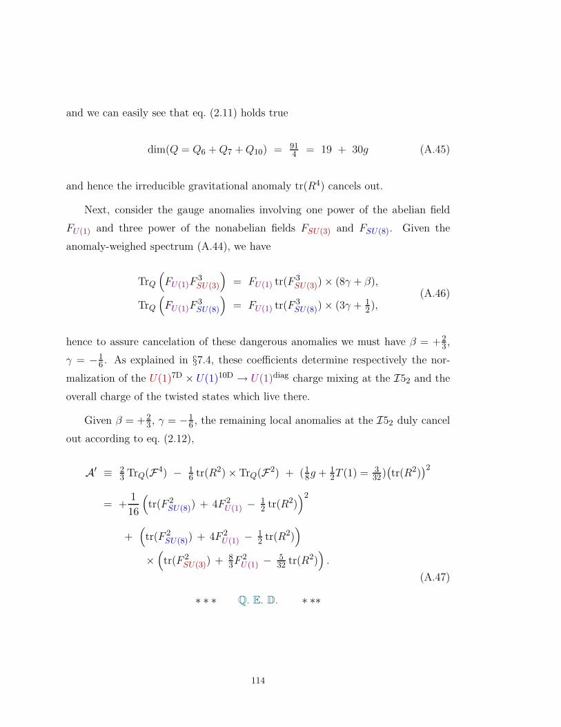
and we can easily see that eq. (2.11) holds true

dim(Q = Q6 +Q7 +Q10) = 914 = 19 + 30g (A.45)

and hence the irreducible gravitational anomaly tr(R4) cancels out.

Next, consider the gauge anomalies involving one power of the abelian field

FU(1) and three power of the nonabelian fields FSU(3) and FSU(8). Given the

anomaly-weighed spectrum (A.44), we have

TrQ

(

FU(1)F3SU(3)

)

= FU(1) tr(F 3SU(3))× (8γ + β),

TrQ

(

FU(1)F3SU(8)

)

= FU(1) tr(F 3SU(8))× (3γ + 1

2),(A.46)

hence to assure cancelation of these dangerous anomalies we must have β = +23 ,

γ = −16 . As explained in §7.4, these coefficients determine respectively the nor-

malization of the U(1)7D × U(1)10D → U(1)diag charge mixing at the I52 and the

overall charge of the twisted states which live there.

Given β = +23 , γ = −1

6 , the remaining local anomalies at the I52 duly cancel

out according to eq. (2.12),

A′ ≡ 23 TrQ(F4) − 1

6 tr(R2)× TrQ(F2) + (18g + 1

2T (1) = 332)(

tr(R2))2

= +1

16

(

tr(F 2SU(8)) + 4F 2

U(1) − 12 tr(R2)

)2

+(

tr(F 2SU(8)) + 4F 2

U(1) − 12 tr(R2)

)

×(

tr(F 2SU(3)) + 8

3F2U(1) − 5

32 tr(R2))

.

(A.47)

∗ ∗ ∗ Q. E. D. ∗ ∗∗

114

REFERENCES

1. P. Horava and E. Witten, “Heterotic and type I string dynamics from eleven

dimensions”, Nucl. Phys. B 460 (1996) 506 [hep-th/9510209].

2. P. Horava and E. Witten, “Heterotic and type I string dynamics from eleven

dimensions”, Nucl. Phys. B 506 (1996) 506 [hep-th/9510209].

3. V. S. Kaplunovsky, J. Sonnenschein, S. Theisen and S. Yankielowicz, “On

the Duality between Perturbative Heterotic Orbifolds and M-Theory on

T 4/ZN”, Nucl. Phys. B 590 (2000) 123 [hep-th/9912144].

4. M. Faux, D. Lust and B. A. Ovrut, “Intersecting orbifold planes and local

anomaly cancellation in M-theory”, Nucl. Phys. B 554 (1999) 437 [hep-

th/9903028].

5. M. Faux, D. Lust and B. A. Ovrut, “Local anomaly cancellation, M-

theory orbifolds and phase-transitions”, Nucl. Phys. B 589 (2000) 269

[hep-th/0005251]; “An M-theory perspective on heterotic K3 orbifold com-

pactifications”, hep-th/0010087; “Twisted sectors and Chern-Simons terms

in M-theory orbifolds”, hep-th/0011031.

6. K. Dasgupta and S. Mukhi, “Orbifolds of M-theory”, Nucl. Phys. B 465

(1996) 399 [hep-th/9512196].

7. E. Witten, “Five-branes and M-Theory on an Orbifold”, Nucl. Phys. B 463

(1996) 383, [hep-th/9512219].

8. G. Aldazabal, A. Font, L. E. Ibanez, A. M. Uranga and G. Violero, “Non-

Perturbative Heterotic D=6, N=1 Orbifold Vacua”, Nucl. Phys. B 519

(1998) 239, [hep-th/9706158].

9. A. Bilal, J.-P. Derendinger and R. Sauser, “M-Theory on S1/Z2: New Facts

from a Careful Analysis”, Nucl. Phys. B 576 (2000) 347 [hep-th/9912150].

10. P. Townsend, “The eleven-dimensional supermembrane revisited”, Phys.

Lett. B 350 (1995) 184 [hep-th/9501068].

115

11. A. Hanany and A. Zaffaroni, “Branes and six-dimensional supersymmetric

theories”, Nucl. Phys. B 529 (1998) 180 [hep-th/9712145]; “Monopoles in

string theory”, JHEP 9912 (1999) 014 [hep-th/9911113].

12. N. Seiberg, “Five dimensional SUSY field theories, non-trivial fixed points

and string dynamics”, Phys. Lett. B 388 (1996) 753 [hep-th/9608111].

13. D. R. Morrison and N. Seiberg, “Extremal transitions and five-dimensional

supersymmetric field theories”, Nucl. Phys. B 483 (1997) 229

[hep-th/9609070].

14. G. Aldazabal, A. Font, L. E. Ibanez and F. Quevedo, “Chains of N=2, D=4

heterotic/type II duals”, Nucl. Phys. B 461 (1996) 85 [hep-th/9510093].

15. M. Duff, R. Minasian and E. Witten, “Evidence for Heterotic/Heterotic

Duality”, Nucl. Phys. B 465 (1996) 413 [hep-th/9601036].

16. J. Polchinski, “String Theory, Vol. II”, Cambridge University Press, 1998.

17. M. Dine, P. Huet and N. Seiberg, “Large And Small Radius In String

Theory”, Nucl. Phys. B 322 (1989) 301.

18. J. Dai, R. G. Leigh and J. Polchinski, “New Connections Between String

Theories”, Mod. Phys. Lett. A 4 (1989) 2073.

19. J. Polchinski and E. Witten, “Evidence for Heterotic - Type I String Duality”,

Nucl. Phys. B 460 (1996) 525 [hep-th/9510169].

20. S. Kachru and E. Silverstein, “On gauge bosons in the matrix model approach

to M theory”, Phys. Lett. B 396 (1997) 70 [hep-th/9612162].

21. D. A. Lowe, “Bound states of type I’ D-particles and enhanced gauge

symmetry”, Nucl. Phys. B 501 (1997) 134 [hep-th/9702006], “Heterotic

matrix string theory”, Phys. Lett. B 403 (1997) 243 [hep-th/9704041].

22. D. Matalliotakis, H. Nilles and S. Theisen, “Matching the BPS spectra of

heterotic – type-I – type-I’ strings”, Phys. Lett. B 421 (1998) 169 [hep-

th/9710247].

116

23. O. Bergman, M. R. Gaberdiel and G. Lifschytz, “String creation and

heterotic-type I’ duality”, Nucl. Phys. B 524 (1998) 524 [hep-th/9711098].

24. C. P. Bachas, M. B. Green and A. Schwimmer, “(8,0) quantum mechanics

and symmetry enhancement in type I’ superstrings”, JHEP 9801 (1998) 006

[hep-th/9712086].

25. F. A. Cachazo and C. Vafa, “Type I’ and real algebraic geometry”, [hep-

th/0001029].

26. M. R. Douglas, S. Katz and C. Vafa, “Small instantons, del Pezzo surfaces

and type I’ theory”, Nucl. Phys. B 497 (1997) 155 [hep-th/9609071].

27. E. Witten, “New “Gauge” Theories In Six Dimension”, JHEP 9801 (1998)

001; Adv. Theor. Math.Phys. 2 (1998) 61 [hep-th/9710065].

28. S. Elitzur, A. Giveon, D. Kutasov, E. Rabinovici and A. Schwimmer “Brane

dynamics and N=1 supersymmetric gauge theories”, Nucl. Phys. B 505

(1997) 202 [hep 9704104]; K. Landsteiner and E. Lopez, “New curves

from branes” Nucl. Phys. B 516 (1998) 273 [hep-th 9708118]; N. Evans,

C.V. Johnson and A.D. Sharpere, “Orientifolds, branes, and duality of 4D

gauge theories”, Nucl. Phys. B 505 (1997) 251 [hep-th 9703210]; A. Brand-

huber, J. Sonnenschein, S. Theisen and S. Yankielowicz, “M theory and

Seiberg-Witten curves: orthogonal and symplectic groups”, Nucl. Phys. B

504 (1997) 175 [hep-th 9705232]; for a review, cf. A. Giveon and D. Ku-

tasov, “Brane dynamics and gauge theory”, Rev. Mod. Phys. 71 (1999) 983

[hep-th/9802067].

29. E. Witten “Solutions of 4d field theories via M-theory”, Nucl./ Phys./ B

500 (1997) 3 [hep-th 9703166].

30. I. Brunner and A. Karch, “Branes at orbifolds versus Hanany Witten in six

dimensions,” JHEP 03 (1998) 003 [hepth/9712143].

31. J.L. Romans, “Massive N=2a Supergravity in 10 Dimensions”, Phys. Lett.

B 169 (1986) 147.

117

32. A. Hanany and E. Witten, “Type IIB superstrings, BPS monopoles, and

three-dimensional gauge dynamics”, Nucl. Phys. B 492 (1997) 152 [hep-

th/9611230].

118