![arXiv:cond-mat/0503477v2 [cond-mat.other] 11 May 2005](https://static.fdocuments.in/doc/165x107/62737c97011391543143743f/arxivcond-mat0503477v2-cond-matother-11-may-2005.jpg)
arXiv:cond-mat/0603637 v1 23 Mar 2006
40
arXiv:cond-mat/0603637 v1 23 Mar 2006 SUPERCONDUCTING QUBITS II: DECOHERENCE F.K. Wilhelm † , M.J. Storcz and U. Hartmann Department Physik, Center for Nanoscience, and Arnold Sommerfeld Cen- ter for theoretical physics, Ludwig-Maximilians-Universit¨ at, 80333 M¨ unchen, Germany Michael R. Geller ‡ Department of Physics, University of Georgia, Athens, Georgia 30602, USA Abstract. This is an introduction to elementary decoherence theory as it is typically applied to superconducting qubits. Abbreviations: SQUID – superconducting quantum interference device; qubit – quan- tum bit; TSS – two state system Contents 1 Introduction 1 2 Single qubit decoherence 11 3 Beyond Bloch-Redfield 25 4 Decoherence in coupled qubits 34 5 Summary 36 6 Acknowledgements 36 1. Introduction The transition from quantum to classical physics, now known as decoher- ence, has intrigued physicists since the formulation of quantum mechanics (Giulini et al., 1996; Leggett, 2002; Peres, 1993; Feynman and Vernon, 1963; Zurek, 1993). It has been put into the poignant Schr¨ odinger cat para- dox (Schr¨ odinger, 1935) and was considered an open fundamental question for a long time. † present address: Physics Department and Insitute for Quantum Computing, Univer- sity of Waterloo, Waterloo, Ontario N2L 3G1, Canada; [email protected] ‡ [email protected] c 2006 Springer. Printed in the Netherlands.
Transcript of arXiv:cond-mat/0603637 v1 23 Mar 2006

arX
iv:c
ond-
mat
/060
3637
v1
23
Mar
200
6
SUPERCONDUCTING QUBITS II: DECOHERENCE
F.K. Wilhelm†, M.J. Storcz and U. HartmannDepartment Physik, Center for Nanoscience, and Arnold Sommerfeld Cen-ter for theoretical physics, Ludwig-Maximilians-Universitat, 80333 Munchen,Germany
Michael R. Geller‡
Department of Physics, University of Georgia, Athens, Georgia 30602, USA
Abstract. This is an introduction to elementary decoherence theory as it is typicallyapplied to superconducting qubits.
Abbreviations: SQUID – superconducting quantum interference device; qubit – quan-tum bit; TSS – two state system
Contents
1 Introduction 12 Single qubit decoherence 113 Beyond Bloch-Redfield 254 Decoherence in coupled qubits 345 Summary 366 Acknowledgements 36
1. Introduction
The transition from quantum to classical physics, now known as decoher-ence, has intrigued physicists since the formulation of quantum mechanics(Giulini et al., 1996; Leggett, 2002; Peres, 1993; Feynman and Vernon,1963; Zurek, 1993). It has been put into the poignant Schrodinger cat para-dox (Schrodinger, 1935) and was considered an open fundamental questionfor a long time.
† present address: Physics Department and Insitute for Quantum Computing, Univer-sity of Waterloo, Waterloo, Ontario N2L 3G1, Canada; [email protected]
c© 2006 Springer. Printed in the Netherlands.

2 F.K. WILHELM, M.J. STORCZ, U. HARTMANN, AND M. GELLER
In this chapter, we study the theory of decoherence as it is appliedto superconducting qubits. The foundations of the methodology used arerather general results of quantum statistical physics and resemble thoseapplied to chemical physics, nuclear magnetic resonance, optics, and othercondensed matter systems (Weiss, 1999). All these realizations introducetheir subtleties — typical couplings, temperatures, properties of the cor-relation functions. We will in the following largely stick to effective spinnotation in order to emphasize this universality, still taking most of theexamples from superconducting decoherence. This paper is based on lec-tures 2 and 3 of the NATO-ASI on “Manipulating quantum coherence insuperconductors and semiconductors” in Cluj-Napoca, Romania, 2005. Itis not intended to be a review summarizing the main papers in the field.Rather, it is an (almost) self-contained introduction to some of the relevanttechniques, aimed to be accessible to researchers and graduate studentswith a knowledge of quantum mechanics (Cohen-Tannoudji et al., 1992)and statistical physics (Landau and Lifshitz, 1984) on the level of a firstgraduate course. So much of the material here is not new and most certainlyknown to more experienced researchers, however, we felt a lack of a singlereference which allows newcomers to get started without excessive overhead.References have largely been chosen for the aid they provide in learning andteaching the subject, rather than importance and achievement.
1.1. BASIC NOTIONS OF DECOHERENCE
The mechanisms of decoherence are usually related to those of energy dis-sipation. In particular, decoherence is irreversible. If we take as an examplea pure superposition state
|ψ〉 = (|0〉 + |1〉)/√
2 ρpure = |ψ〉〈ψ| =1
2
(
1 11 1
)
(1)
and compare it to the corresponding classical mixture leading to the sameexpectation value of σz
ρmix =1
2
(
1 00 1
)
(2)
we can see that the von-Neumann entropy ρ = −kBTr [ρ log ρ] rises fromSpure = 0 to Smix = kB ln 2. Hence, decoherence taking ρpure to ρmix createsentropy and is irreversible.
Quantum mechanics, on the other hand, is always reversible. It canbe shown, that any isolated quantum system is described by the Liouvillevon-Neumann equation
ihρ = [H, ρ] (3)

SUPERCONDUCTING QUBITS II: DECOHERENCE 3
which conserves entropy. Indeed, also the CPT theorem of relativistic quan-tum mechanics (Sakurai, 1967) states, that for each quantum system it ispossible to find a counterpart (with inversed parity and charge) whosetime arrow runs backwards. The apparent contradiction between microre-versibility — reversibility of the laws of quantum physics described bySchrodinger’s equation — and macro-irreversibility is a problem at thefoundation of statistical thermodynamics. We also remark that the La-grangian formalism (Landau and Lifshitz, 1982) which was used as thestarting point in the previous chapter of this book (Geller et al., 2006) doesnot even accomodate friction on a classical level without artificial and ingeneral non-quantizable additions.
1.1.1. Heat baths and quantum Brownian motionThe standard way out of this dilemma is to introduce a continuum of ad-ditional degrees of freedom acting as a heat bath for the quantum systemunder consideration (Feynman and Vernon, 1963; Caldeira and Leggett,1981; Caldeira and Leggett, 1983). The complete system is fully quantum-coherent and can be described by equation 3. However, the heat bathcontains unobserved degrees of freedom which have to be integrated outto obtain the reduced system; the reduced system is the original quantumsystem which does not contain the bath explicitly, but whose dynamics areinfluenced by the bath. The dynamics of the reduced system now show bothdissipation (energy exchange with the heat bath) and decoherence (loss ofquantum information to the heat bath). Another view on this is that anyfinite combined quantum system shows dynamics which are periodic intime. The typical periods are given by the inverse level splittings of thesystem. Thus, a continuous heat bath shows periodicity and reversibilityonly on an infinite, physically unobservable time scale.
A standard example, taken from Ref. (Ingold, 1998), of irreversibilityin both classical and quantum mechanics is (quantum) Brownian motion(QBM), which we will now describe in the one-dimensional case. The under-lying Hamiltonian of a single particle in an oscillator bath has the generalstructure
H = Hs +Hsb +Hb +Hc. (4)
Here, the system Hamiltonian Hs describes an undamped particle of mass
M in a scalar potential, Hs = P 2
2M +V (q). Hb describes a bath of harmonic
oscillators, Hi =∑
i
(
p2i
2mi+ 1
2miω2i x
2i
)
. The coupling between these two
components is bilinear, Hsb = −q∑i cixi. If this were all, the effectivepotential seen by the particle would be altered even on the classical level,as will become more obvious later on. Thus, we have to add a counter term

4 F.K. WILHELM, M.J. STORCZ, U. HARTMANN, AND M. GELLER
which does not act on the bath, Hc = q2∑
ic2i
2miω2i. Adding this counterterm
gives the Hamiltonian the following intuitive form
H =P 2
2M+ V (q) +
∑
i
p2i
2mi+
1
2miω
2i
(
xi −ci
miω2i
q
)2
(5)
indicating that the bath oscillators can be viewed as attached to the particleby springs. Here, we have introduced sets of new parameters, ci, ωi, andmi which need to be adjusted to the system of interest. This aspect will bediscussed later on. We treat this system now using the Heisenberg equationof motion
ihO(t) = [O(t),H] (6)
for the operators q, P , xi, and pi, which (as a mathematical consequenceof the correspondence principle) coincide with the classical equations ofmotion. The bath oscillators see the qubit acting as an external force
xi + ω2i xi =
cimiq(t). (7)
This equation of motion can be solved by variation of constants, which canbe found in textbooks on differential equations such as (Zill, 2000)
xi(t) = xi(0) cos ωit+pi(0)
miωisinωit+
c2imiω2
i
∫ t
0dt′ sinωi(t− t′)q(t′) (8)
Analogously, we find the equation of motion for the particle
q = −∂V∂q
−∑ ci
mixi − q
∑ c2imiω2
i
. (9)
Substituting eq. 8 into eq. 9 eliminates the bath coordinates up to the initialcondition
Mq = −∂V∂q
−∑
i
c2imiωi
∫ t
0dt′ sinωi(t− t′)q(t′)
+∑
i
ci
(
xi(0) cos ωit+pi(0)
miωisinωit
)
− q∑
i
c2imiω2
i
. (10)
We now integrate by parts and get a convolution of the velocity plus bound-ary terms, one of which shifts the origin of the initial position, the othercancels the counterterm (indicating, that without the counterterm we wouldobtain a potential renormalization). The result has the compact form
Mq +∂V
∂q+
∫ t
0dt′γ(t− t′)q(t′) = ξ(t). (11)

SUPERCONDUCTING QUBITS II: DECOHERENCE 5
This structure is identified as a Langevin equation with memory friction. Ifinterpreted classically, this is the equation of motion of a Brownian particle- a light particle in a fluctuating medium. In the quantum limit, we haveto read q, xi and the derived quantity ξ as operators. We see both sides ofopen system dynamics — Dissipation encoded in the damping kernel γ anddecoherence encoded in the noise term ξ. We can express γ as
γ(t) =∑
i
c2imiω2
i
cosωit =
∫ ∞
0
dω
ωJ(ω) cos ωt (12)
where we have introduced the spectral density of bath modes
J(ω) =∑
i
c2imiωi
δ(ω − ωi) (13)
which is the only quantifier necessary to describe the information encodedin the distribution of the mi, ωi, and ci. The right hand side of eq. 11 is anoise term and reads
ξ(t) =∑
i
ci
[(
xi(0) −ci
miω2i
q(0)
)
cosωit+pi(0)
miωisinωit
]
. (14)
This crucially depends on the initial condition of the bath. If we assumethat the bath is initially equilibrated around the initial position q(0) ofthe particle, we can show, using the standard quantum-statistics of thesimple harmonic oscillator, that the noise is unbiased, 〈ξ(t)〉 = 0, and itscorrelation function is given by
K(t) = 〈ξ(t)ξ(0)〉 =
∫
dωJ(ω) [cosωt (2n(hω) + 1) − i sinωt] (15)
where n is the Bose function, n(hω) = (ehω/kT − 1)−1, and 2n(hω) + 1 =
coth(
hω2kBT
)
. Here and henceforth, angular brackets around an operator
indicate the quantum-statistical average, 〈O〉 = Tr(ρO) with ρ being theappropriate density matrix. We will get back to the topic of the initialcondition in section 3.1.2 of this chapter.
The noise described by ξ(t) is the quantum noise of the bath. In partic-ular, the correlation function is time-translation invariant,
K(t) = 〈ξ(t+ τ)ξ(τ)〉 (16)
but not symmetric
K(−t) = 〈ξ(0)ξ(t)〉 = K∗(t) 6= K(t). (17)

6 F.K. WILHELM, M.J. STORCZ, U. HARTMANN, AND M. GELLER
which reflects the fact that ξ as defined in eq. 14 is a time-dependentoperator which does generally not commute at two different times. Ex-plicitly, the imaginary part of K(t) changes its sign under time reversal.Indeed, if the derivation of eq. 15 is done explicitly, one directly sees thatit originates from the finite commutator. Moreover, we can observe thatat T ≫ ω we have 2n + 1 → 2kBT/hω ≫ 1, thus the integral in eq, 15 isdominated by the symmetric real part now describing purely thermal noise.At any temperature, the symmetrized semiclassical spectral noise power infrequency space reads
S(ω) =1
2〈ξ(t)ξ(0) + ξ(0)ξ(t)〉ω = S(−ω) (18)
where 〈. . .〉ω means averaging and Fourier transforming. This quantity con-tains a sign of the quantum nature of noise. Unlike classical noise, it doesnot disappear at low temperatures T ≪ hω/kB , but saturates to a finitevalue set by the zero-point fluctuations, whereas at high temperature werecover thermal noise. Note, that the same crossover temperature dictatesthe asymmetry in eq. (17). Both observations together can be identified withthe fact, that zero-point fluctuations only allow for emission of energy, notabsorption, as will be detailed in a later section of this chapter.
Our approach in this chapter is phenomenological. The main param-eter of our model is the spectral density J(ω). We will show in sections1.1.3, 2.1.1 and 2.1.2 how J(ω) can be derived explicitly for Josephsonjunction circuits. Oscillator baths accurately model numerous other situa-tions. Decoherence induced by phonons in quantum dot systems allows todirectly identify the phonons as the bath oscillators (Brandes and Kramer,1999; Storcz et al., 2005a), whereas in the case of electric noise from resistorsor cotunneling in dots (Hartmann and Wilhelm, 2004) it is less obvious— the Bosons are electron-hole excitations, which turn out to have thecommutation relation of hard-core bosons (von Delft and Schoeller, 1998)with the hard-core term being of little effect in the limits of interest (Weiss,1999).
Going back to our phenomenology, we introduce the most importantcase of an Ohmic bath
J(ω) = γωf(ω/ωc). (19)
Here, γ is a constant of dimension frequency and f is a high-frequency cutofffunction providing f(x) ≃ 1 at x < 1 and f → 0 at x > 1. Popular choicesinclude the hard cutoff, f(x) = θ(1 − x), exponential cutoff, f(x) = e−x,and the Drude cutoff f(x) = 1
1+x2 . We will see in section 1.1.3 that theDrude cutoff plays a significant role in finite electrical circuits, so we choseit here for illustration purposes. In this case, the damping kernel reduces

SUPERCONDUCTING QUBITS II: DECOHERENCE 7
toγ(τ) = γωce
−ωcτ . (20)
For ωc → ∞, γ becomes a delta function and we recover the classicaldamping with damping constant γ, γ(τ) = γδ(τ). Here, “classical damping”alludes to the damping of particle motion in fluid or of charge transportin a resistor (thus the name Ohmic, see also section 1.1.3). With finiteωc, the Ohmic models leads to classical, linear friction proportional to thevelocity, smeared out over a memory time set by the inverse cutoff frequencydefining a correlation time tc = ω−1
c . On the other hand, as it turns out inthe analysis of the model e.g. in section 2.2.2, an infinite cutoff always leadsto unphysical divergencies. Examples will be given later on. All examplesfrom the class of superconducting qubits have a natural ultraviolet cutoffset by an appropriate 1/RC or R/L with R, L, and C being characteristicresistances, inductances, and capacitances of the circuit, respectively. Note,that parts of the open quantum systems literature do not make this lastobservation.
We will not dwell on methods of solution of the quantum Langevin equa-tion, as the focus of this work is the decoherence of qubit systems. Methodsinclude the associated Fokker-Planck equation, path integrals, and quantumtrajectory simulations. The quantum Langevin equation finds application inthe theory of quantum decay in chemical reactions, the dissipative harmonicoscillator, and the decoherence of double-slit experiments.
1.1.2. How general are oscillator baths?Even though the model introduced looks quite artificial and specific, itapplies to a broad range of systems. The model essentially applies as longas the heat bath can be treated within linear response theory, meaning thatit is essentially infinite (i.e. cannot be exhausted), has a regular spectrum,and is in thermal equilibrium. We outline the requirement of only weaklyperturbing the system, i.e. of linear response theory (Kubo et al., 1991).The derivation is rather sketchy and just states the main results becausethis methodology will not be directly used later on. Introductions can befound e.g. in Ref. (Kubo et al., 1991; Ingold, 1998; Callen and Welton,1951)
In linear response theory, we start from a Hamiltonian H0 of the oscil-lator bath which is perturbed by an external force F coupling to a bathoperator Q,
H = H0 − FQ (21)
where the perturbation must be weak enough to be treated to lowest order.It is a result of linear response theory that the system responds by a shift

8 F.K. WILHELM, M.J. STORCZ, U. HARTMANN, AND M. GELLER
of Q (taken in the Heisenberg picture) according to
〈δQ(t)〉ω = χ(ω)F (ω) (22)
where the susceptibility χ can be computed to lowest order as the correla-tion function
χ = 〈Q(0)Q(0)θ(t)〉ω (23)
computed in thermal equilibrium. We can split the correlation functioninto real and imaginary parts χ = χ′ + iχ′′. The real part determines thefluctuations, i.e.
1
2〈δQ(t)δQ(0) + δQ(0)δQ(t)〉ω = χ′ (24)
whereas the imaginary part determines the energy dissipation
〈E(t)〉ω = ωχ′′|F |2. (25)
together with the equations 12 and 18 tracing both damping and noiseback to a single function χ constitute the famous fluctuation-dissipationtheorem (Callen and Welton, 1951), a generalization of the Einstein relationin diffusion.
In this very successful approach we have characterized the distributionof the observableQ close to thermal equilibrium by its two-point correlationfunction alone. This is a manifestation of the fact that its distribution,following the central limit theorem is Gaussian, i.e. can be characterizedby two numbers only: mean and standard deviation. Oscillator baths pro-vide exactly these ingredients: by properly chosing J(ω) they can be fullyadjusted to any χ(ω), and all higher correlation functions — correlationfunctions involving more than two operators — can also be expressedthrough J hence do not contain any independent piece of information.
This underpins the initial statement that oscillator baths can describe abroad range of environments, including those composed of Fermions and notBosons, such as a resistor. As explained in section 1.1.1, the oscillators areintroduced artifically — on purely statistical grounds as a tool to describefluctuations and response — and can only sometimes be directly identifiedwith a physical entity.
There are still a number of environments where the mapping on anoscillator bath is in general not correct. These include i) baths of uncoupledspins (e.g. nuclear spins), which are not too big and can easily saturate,i.e. explore the full finite capacity of their bounded energy spectrum ii)shot noise, which is not in thermal equilibrium iii) nonlinear electricalcircuits such as many Josephson circuits and iv) in most cases 1/f noise,

SUPERCONDUCTING QUBITS II: DECOHERENCE 9
whose microscopic explanation either hints at non-Gaussian (spin-like) ornonequilibrium sources as discussed in section 3.1.3.
1.1.3. Oscillator bath models for Josephson junction devicesWe have now learned two approaches to characterize the oscillator bath:through noise, and through friction. We will now apply the characterizationby friction to a simple Josephson circuit with Josephson energy EJ, junctioncapacitance CJ and arbitrary shunt admittance in parallel, all biased by anexternal current IB. We are extending the method presented in the previouschapter (Geller et al., 2006) to include the admittance. We start with theelementary case of a constant conductance, Y (ω) = G. The total currentsplits up into the three elements as
IB = Ic sinφ+ CΦ0
2πφ+G
Φ0
2πφ. (26)
Reordering terms, we can cast this into the shape of Newton’s equation fora particle with coordinate φ.
C
(
Φ0
2π
)2
φ+G
(
Φ0
2π
)2
φ+∂V
∂φ= 0. (27)
Here, we have multiplied the equation by another Φ0/2π to ensure properdimensions of the potential energy
V (φ) = −IBΦ0
2πφ+ EJ(1 − cosφ) (28)
where we have introduced the Josephson energy EJ = I0Φ0/2π. This ex-pression can be readily compared to eq. 11. We see that the friction termhas no memory, i.e. γ(t) ∝ δ(t), and using the results of section 1.1.1 wecan infer that J(ω) = G(Φ0/2π)ω, i.e. an Ohmic resistor leads naturallyto an Ohmic spectral density as mentioned before. Note that this has nocutoff, but any model of an Ohmic resistor leads to reactive behavior athigh frequencies.
We see that we missed the noise term on the right, which would representcurrent noise originating in G and which would have to be included in amore sophisticated circuit analysis which careful engineers would do. Byapplying the fluctuation dissipation theorem to γ we can add on the propernoise term, whose correlation function is given by equation (15) — or wecan simply use this equation with the J(ω) obtained.
We want to generalize this system now to an arbitrary shunt admittanceY (ω). For that, it comes in handy to work in Fourier space and we denote

10 F.K. WILHELM, M.J. STORCZ, U. HARTMANN, AND M. GELLER
the Fourier transform by F . Analogous to eq. (27), we can find the followingexpression
− ω2C
(
Φ0
2π
)2
φ+ iωY (ω)
(
Φ0
2π
)2
φ+ F(
∂V
∂φ
)
= 0. (29)
We have to remember that the damping Kernel γ is the Fourier cosinetransform of J(ω)/ω, which also implies that it is a real valued function.We can split Y into real (dissipative) and imaginary (reactive) parts Y =Yd + iYr. For any finite electrical circuit, Yd is always an even and Yr alwaysan odd function of frequency. All this allows us to rewrite eq. 29
− ω2C
(
Φ0
2π
)2
φ− ωYr(ω)
(
Φ0
2π
)2
φ+ iωYd(ω)
(
Φ0
2π
)2
φ+ F(
∂V
∂φ
)
= 0.
(30)Thus, the general expression for the spectral density reads J(ω) = ωYd =ωReY (ω), i.e. it is controlled by the dissipative component of Y (ω) alone.There is a new term containing the reactive component Yr which modifiesthe non-dissipative part of the dynamics and can lead e.g. to mass orpotential renormalization, or something more complicated. Comparing thisresult to the structure of the susceptibility χ in the discussion of section1.1.2 it looks like the real and imaginary part have changed their role andthere is an extra factor of ω. This is due to the fact that Y links I and V ,whereas the energy-valued perturbation term in the sense of section 1.1.2is QV . This aspects adds a time-derivative Y = χ which leads to a factoriω in Fourier space.
This last result can be illustrated by a few examples. If Y (ω) = GΦ0/2π,we recover the previous equation (27). If the shunt is a capacitor Cs, wehave Y (ω) = iωCs and we get from eq. (30) the equation of motion ofa particle with larger mass, parameterized by a total capacitance Ctot =CJ + Cs. On the other hand, if the shunt is an inductance Ls, we obtainY (ω) = (iωLs)
−1, leading to a new contribution to the potential originatingfrom the inductive energy
Vtot(φ) = V (φ) +(Φ0)
2
8π2Lφ2 (31)
and no damping term. Finally, let us consider the elementary mixed caseof a shunt consisting of a resistor Rs and a capacitor Cs in series. Wefind Y (ω) = iωCs
1+iωRsCswhich can be broken into a damping part which is
supressed below a rolloff frequency ωr = (RC)−1, Yd1R
11+ω2/ω2
rand a reac-
tive part which responds capacitively below that rolloff, Yr = iωC 11+ω2/ω2
r.
As the rolloffs are very soft, there is no straightforward mapping onto a

SUPERCONDUCTING QUBITS II: DECOHERENCE 11
very simple model and we have to accept that the dynamics get morecomplicated and contain a frequency-dependent mass and friction as wellas time-correlated noise, all of which gives rise to rich physics (Robertsonet al., 2005).
2. Single qubit decoherence
2.1. TWO-STATE OSCILLATOR BATH MODELS
In the previous section, we introduced the notion of an oscillator bath envi-ronment for continuous systems including biased Josephson junctions. Wederived quantum Langevin equation demonstrating the analogy to classicaldissipative motion, but did not describe how to solve them. In fact, solvingthese equations in all generality is extremely hard in the quantum limit,thus a restriction of generality is sought. For our two-state systems (TSS) ofinterest, qubits, we are specifically interested in the case where the potentialin the Hamiltonian of eq. 5 forms a double well with exactly one boundstate per minimum, tunnel-coupled to each other and well separated fromthe higher excited levels, (Geller et al., 2006). When we also concentrate onthe low-energy dynamics, we can replace the particle coordinate q by q0σz
and the Hamiltonian reads
H =ǫ
2σz +
∆
2σx +
σz
2
∑
i
λi(ai + a†i ) +∑
i
ωi(a†iai + 1/2), (32)
where ǫ is the energy bias and ∆ is the tunnel splitting. This is the fa-mous Spin-Boson Hamiltonian (Leggett et al., 1987; Weiss, 1999). We havedropped the counterterm, which is ∝ q2 in the continuous limit and, dueto q = ±q0 is constant in the two-state case. The spectral density isconstructed out of the J(ω) in the continuous limit
JTSS =∑
i
λ2i δ(ω − ωi) =
q202πh
J(ω) (33)
The Spin-Boson Hamiltonian, eq. (33) is more general than the truncationof the energy spectrum in a double-well potential may suggest. In fact,it can be derived by an alternative procedure which performs the two-state approximation first (or departs from a two-state Hamiltonian withoutasking for its origin) and then characterizes the bath. The oscillator bathapproximation holds under the same conditions explained in section 1.1.2The Spin-Boson model makes the assumption, that each oscillator couplesto the same observable of the TSS which can always be labelled σz. This is

12 F.K. WILHELM, M.J. STORCZ, U. HARTMANN, AND M. GELLER
a restrictive assumption which is not necessarily true for all realizations ofa dissipative two-state system.
As the two-state counterpart to classical friction used in the continuouscase is not straightforward to determine, the environmental spectrum iscomputed from the semiclassical noise of the environment, following theprescription that, if we rewrite eq. 32 in the interaction picture with respectto the bath as
HI =ǫ+ δǫ(t)
2σz +
∆
2σx +
∑
i
ωi(a†iai + 1/2) (34)
we can identify δǫ for any physical model mapping on the Spin-Boson modelas
1
2〈δǫ(t)δǫ(0) + δǫ(0)δǫ(t)〉ω = JTSS(ω) coth
(
hω
2kBT
)
(35)
An application of this procedure will be presented in the next subsection.
2.1.1. Characterization of qubit environments through noiseA standard application of the characterization of the environment is thedescription of control electronics of relatively modest complexity, attachedto a flux qubit. We look at the definite example shown in 2.1.1. It showsa simplified model of the microwave leads providing the control of a fluxqubits. The microwaves inductively couple to the sample by a mutual in-ductance M between the qubit and a coil with self-inductance L. Theseleads are mounted in the cold part of the cryostat, usually on the qubitchip, and are connected to the outside world by a coaxial line which almostinevitably has an impedance of Z = 50Ω. That impedance provides — inlight of the discussion in the previous section — a significant source ofdamping and decoherence. As a design element, one can put two resistorsof size R close to the coil.
The environmental noise is easily described by the Nyquist noise (Callenand Welton, 1951) of the voltage V between the arms of the circuit, seefigure 2.1.1. The Johnson-Nyquist formula gives the voltage noise
SV =1
2〈V (t)V (0) + V (0)V (t)〉 = hωReZeff coth
(
hω
2kBT
)
(36)
where Zeff is the effective impedance between the arms, here of a parallelsetup of a resistor and an inductor
Zeff =iωLeffR
R+ iωLeff, (37)
and Leff is the total impedance of the coupled set of conductors as seenfrom the circuit. For microwave leads, the total inductance is dominatedby the self-inductance of the coil, hence Leff ≈ L.
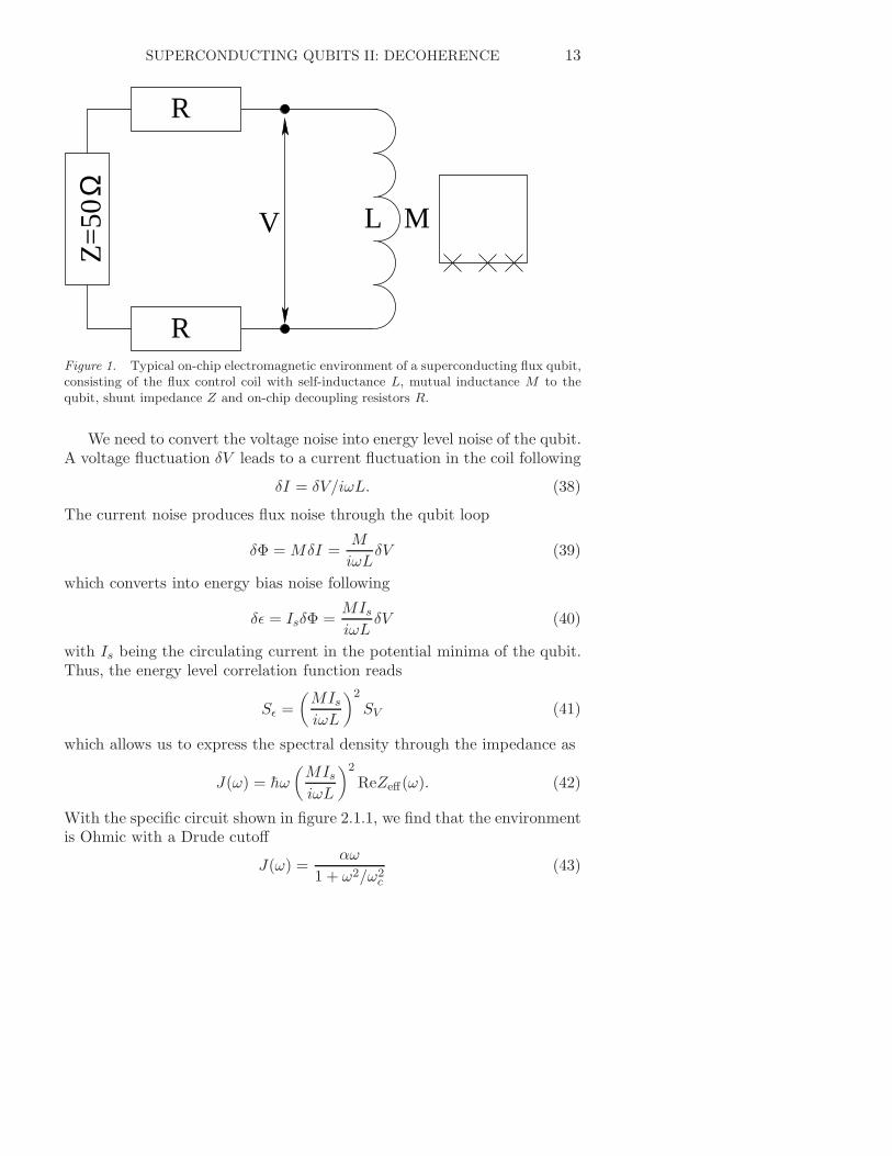
SUPERCONDUCTING QUBITS II: DECOHERENCE 13
Z=
50 Ω
V L M
R
R
Figure 1. Typical on-chip electromagnetic environment of a superconducting flux qubit,consisting of the flux control coil with self-inductance L, mutual inductance M to thequbit, shunt impedance Z and on-chip decoupling resistors R.
We need to convert the voltage noise into energy level noise of the qubit.A voltage fluctuation δV leads to a current fluctuation in the coil following
δI = δV/iωL. (38)
The current noise produces flux noise through the qubit loop
δΦ = MδI =M
iωLδV (39)
which converts into energy bias noise following
δǫ = IsδΦ =MIsiωL
δV (40)
with Is being the circulating current in the potential minima of the qubit.Thus, the energy level correlation function reads
Sǫ =
(
MIsiωL
)2
SV (41)
which allows us to express the spectral density through the impedance as
J(ω) = hω
(
MIsiωL
)2
ReZeff(ω). (42)
With the specific circuit shown in figure 2.1.1, we find that the environmentis Ohmic with a Drude cutoff
J(ω) =αω
1 + ω2/ω2c
(43)

14 F.K. WILHELM, M.J. STORCZ, U. HARTMANN, AND M. GELLER
with ωc = L/R and α = 4M2I2s
h(Z+2R) . Thus, we find a simple method to engineer
the decoherence properties of thw circuit with our goal being to reduceJ(ω) by decoupling the device from the shunt Z. The method of choice isto put large resistors R on chip. Their size will ultimately be limited by thenecessity of cooling them to cryogenic temperatures. The friction methodintroduced earlier, section 1.1.3 , leads to the same result.
2.1.2. Linearization of nonlinear environmentsIn general, nonlinear environments important for qubit devices can alsobe identified. In superconducting devices, these include electronic environ-ments which in addition to the linear circuit elements discussed in theprevious section, also contain Josephson junctions. In general, such envi-ronments cannot be described by oscillator bath models, whose responsewould be strictly linear. Here, we want to concentrate on the case of anonlinear environment — a SQUID detector — in the regime of small signalresponse, i.e. in a regime where it can be linearized. This linearization can beillustrated by the concept of Josephson inductance. Let us remind ourselves,that a linear inductor is defined through the following current-flux relation
I(Φ) = Φ/L (44)
whereas the small flux-signal response of a Josephson junction can beapproximated as
I = sin
(
2πΦ
Φ0
)
≃ Ic sin
(
2πΦ
Φ0
)
+δΦ
LJ(45)
where we have split the flux into its average Φ and small deviations δΦ andhave introduced the Josephson inductance LJ = Φ0/2πIc cos φ. Thus, thesmall-signal response is inductive.
We would now like to demostrate this idea on the example of a DC-SQUID detector inductively coupled to the qubit, see fig. 2.1.2.
In the first stage, we again need to find the voltage noise between thebranches of the circuit. This is given by eq. (36) with the appropriateinductance calculated from the cicruit shown in the lower panel of fig. 2.1.2,Z−1
eff = R−1 + iωC + (iωLJ)−1. This is the impedance of an LC resonatorwith damping. The conversion into energy level noise goes along similarlines as before, incorporating the SQUID equations as described here andin standard literature (Tinkham, 1996; Clarke and Braginski, 2004).
The DC-SQUID is a parallel setup of two Josephson junctions 1 and 2,which for simplicity are assumed to be identical. The total current flowingthrough the device is
IB = Ic(sinφ1 + sinφ2) = 2Ic cos(δφ/2) sin φ (46)

SUPERCONDUCTING QUBITS II: DECOHERENCE 15
bias
circI
C
R V I
biasLJ C
R V I
Figure 2. Upper panel: DC-SQUID readout circuit consisting of the actual SQUID, ashunt capacitor, and a voltmeter with an unavoidable resistor. Lower panel: Linearizedcircuit used for the noise calculation
where we have introduced φ = (φ1 +φ2)/2 and δφ = φ1 −φ2. Now we needto remember that the phases φi are connected to the Schrodinger equa-tion for the superconducting condensate. Thus, an elementary calculation(Tinkham, 1996; Clarke and Braginski, 2004) leads to
δφ = 2πΦ
Φ0mod2π (47)
where Φ is the total magnetic flux through the loop. This is identical to theflux applied externally using a biasing coil plus the qubit flux as we neglectself-inductance. Thus, for the bias current IB the DC-SQUID acts like a tun-able Josephson junction with a critical current Ic,eff(Φ) = 2Ic| cos(πΦ/Φ0)|.Thus, we can translate voltage fluctuations into phase fluctuations as
δφ =
(
2π
Φ0
)
δV
iω. (48)

16 F.K. WILHELM, M.J. STORCZ, U. HARTMANN, AND M. GELLER
The qubit is coupling to the magnetic flux which — assuming a symmetricSQUID geometry - is coupled only to the circulating current
Icirc = Ic(sin φ1 − sinφ2)/2 = Ic cos(φ) sinπΦ
Φ0. (49)
We can now express its fluctuations through the fluctuations of φ
δIcirc = −Ic sinπΦ
Φ0sin(φ)δφ =
IB2
tanπΦ
Φ0δφ (50)
where in the last step we have used eq. 46. With the remaining stepsanalogous to the previous section, we obtain
J(ω) = hω
(
MIsIB2
2π
Φ0tan
πΦ
Φ0
)2
ReZeff . (51)
Here, Zeff is the impedance of the linearized circuit shown in the bottompanel of fig. 2.1.2. This result reveals a few remarkable features. Mostprominently, it shows that J(ω) can be tuned by shifting the working pointof the linearization through changing the bias current IB . In particular,J(ω) can be set to zero by chosing IB = 0. The origin of this decouplingcan be seen in eq. 50, which connects the bias current noise to the circulatingcurrent noise. The physical reason for this is, that in the absence of a biascurrent the setup is fully symmetric — any noise from the external circuitrysplits into equal amounts on the branches of the loop and thus does notlead to flux noise. For a detector, this is a highly desired property. It allowsto switch the detector off completely. When we do not bias, we have (forthe traditional switching current measurement) no senitivity and with it nobackaction. This means, that if the device is really highly symmetric, onecan push this device to the strong measurement regime while still being ableto operate in the ”off” state of the detector. This effect has been predictedin Refs. (van der Wal et al., 2003; Wilhelm et al., 2003). Experimentally, itwas first observed that the decoupled point was far from zero bias due toa fabrication issue (Burkard et al., 2005), which was later solved such thatour prediction has indeed been verified (Bertet et al., 2005a).
2.1.3. The Bloch equationSo far, we have discussed the characterization of the environment at length.We did not specify how to describe the qubit dynamics under its influence.For a continuous system, we have derived the quantum Langevin equa-tion (11). Even though this eqution looks straightforward, solving it forpotentials others than the harmonic oscillator is difficult without furtherapproximations. We will now show first how to describe decoherence in

SUPERCONDUCTING QUBITS II: DECOHERENCE 17
a phenomenological way and then discuss how to reconcile microscopicmodelling with the Bloch equation.
For describing the decoherence of a qubit we have to use the densitymatrix formalism. which can describe pure as well as mixed states. Inthe case of a qubit with a two-dimensional Hilbert space, we can fullyparameterize the density matrix by its three spin projections Si = Tr(ρσi),i = x, y, z as
ρ =1
2
(
1 +∑
i
Siσi
)
(52)
where the σi are Pauli matrices. This notation is inspired by spin reso-nance and is applicable to any two-state system including those realizedin superconducting qubits. We can take the analogy further and use thetypical NMR notation with a strong static magnetic field Bz(t) appliedin one direction identified as the z-direction and a small AC field, Bx(t)and By(t) in the xy-plane. In that case, there is clearly a preferred-axissymmetry and two distinct relaxation rates, the longitudinal rate 1/T1 andthe transversal rate 1/T2 can be introduced phenomenologically to yield
Sz = γ( ~B × ~S)z −Sz − Sz,eq
T1(53)
Sx/y = γ( ~B × ~S)x/y −Sx/y
T2(54)
where we have introduced the equilibrium spin projection Sz,eq and the
spin vector ~S = (Sx, Sy, Sz)T . Note that the coherent part of the time
evolution is still present. It enters the Bloch equation via the Hamiltonian,decomposed into Pauli matrices as H = −γ ~B · ~S. This spin notation is alsouseful for superconducting qubits, even though the three components usu-ally depend very distinct observables such as charge, flux, and current. Thisparameterization leads to the practical visualization of the state and theHamiltonian as a point and an axis in three-dimensional space respectively.The free evolution of the qubit then corresponds to Larmor precessionaround the magnetic field. The pure states of the spin have ~S2 = 1 andare hence on a unit sphere, the Bloch sphere, whereas the mixed states areinside the sphere — in the Bloch ball.
The rates are also readily interpreted in physical terms. As the largestatic field points in the z-direction in our setting, the energy dissipation isgiven as
d〈E〉dt
= −γBzSz (55)

18 F.K. WILHELM, M.J. STORCZ, U. HARTMANN, AND M. GELLER
and hence its irreversible part is given through 1/T1. On the other hand,the purity (or linearized entropy) P = Trρ2 = 1/4 +
∑
i S2i decays as
P = 2∑
i
SiSi = −S2
x + S2y
T2− Sz(Sz − Sz,eq)
T1(56)
thus all rates contribute to decoherence. Note, that at low temperaturesSz,eq → 1 so the T1-term in general augments the purity and reestablishescoherence. This can be understood as the system approaches the groundstate, which is a pure state. In this light, it needs to be imposed that P ≤ 1as otherwise the density matrix has negative eigenvalues. This enforcesT2 ≤ 2T1.
2.2. SOLUTIONS OF THE BLOCH EQUATION AND SPECTROSCOPY
The rates shown in the Bloch equation are also related to typical spectro-copic parameters (Abragam, 1983; Goorden and Wilhelm, 2003). We chosea rotating driving field
Bx = (ωR/γ) cos ωt (57)
By = (ωR/γ) sinωt. (58)
In spectroscopy, we are asking for the steady state population, i.e. for thelong-time limit of Sz. Transforming the Bloch equation into the frame co-rotating with the driving field and computing the steady-state solution, weobtain
Sz(ω) =ω2
R
(ω − γB)2 + γ2(59)
with a linewidth γ2 = 1/T 22 + ω2
RT2/T1. This simple result allows spectro-scopic determination of all the parameters of the Bloch equation: At weakdriving, ωR
√T1T2 ≪ 1, the line width is 1/T2. This regime can be easily
identified as the spectral line not being saturated, i.e. the height grows withincreasing drive. In fact, the height of the resonance is Sz(γB) = ω2
RT22 ,
which (knowing 1/T2) allows to determine ωR. Due to the heavy filteringbetween the room-temperature driving and the cryogenic environment, thisis not known a priory. To determine T1, one goes to the high driving regimewith a saturated line, i.e. a line which does not grow any more with higherpower, ωR
√T1T2 ≫ 1 and finds a line width of ωR
√
T1/T2. With all otherparameters known already, this allows to find T1. Using this approach ishelpful to debug an experiment which does not work yet. Alternatively,real-time measurements of T1 are possible under a wide range of conditions.
SUPERCONDUCTING QUBITS II: DECOHERENCE 19
2.2.1. How to derive the Bloch equation: The Bloch-Redfield techniqueWe now show how to derive Bloch-like equations from the system-bathmodels we studied before using a sequence of approximations. The Bornapproximation works if the coupling between system and bath is weak. TheMarkov approximation works if the coupling between system and bath isthe slowest process in the system, in particular if it happens on a time scalelonger than the correlation time of the environment. Quantitatively, we canput this into the motional narrowing condition
λτch
≪ 1 , (60)
where λ is the coupling strength between the system and its environmentand τc the correlation time of the environment. In the case treated in eq.19 we would have τc = 1/ωc. If this is satisfied, an averaging process overa time scale longer than τc but shorter than λ−1 can lead to simple evolu-tion equations, the so-called Bloch-Redfield equations (Argyres and Kelley,1964). The derivation in Ref. (Cohen-Tannoudji et al., 1992) follows thisinspiration. We will follow the very elegant and rigorous derivation usingprojection operators as given in (Argyres and Kelley, 1964; Weiss, 1999).We are going to look at a quantum subsystem with an arbitrary finitedimensional Hilbert space, accomodating also qudit and multiple-qubitsystems.
As a starting point for the derivation of the Bloch-Redfield equations(70), one usually (Weiss, 1999) takes the Liouville equation of motion forthe density matrix of the whole system W (t) (describing the time evolutionof the system)
W (t) = − i
h[Htotal,W (t)] = LtotalW (t) , (61)
where Htotal is the total Hamiltonian and Ltotal the total Liouvillian ofthe whole system. This notation of the Liouvillian uses the concept ofa superoperator. Superoperator space treats density matrices as vectors.Simply arrange the matrix elements in a column, and each linear operationon the density matrix can be written as a (super)matrix multiplication.Thus, the right hand side of the Liouville equation can be written as asingle matrix products, not a commutator, where a matrix acts from theleft and the right at the same time. Hamiltonian and Liouvillian consist ofparts for the relevant subsystem, the reservoir and the interaction betweenthese
Htotal = Hsys +Hres +HI (62)
Ltotal = Lsys + Lres + LI . (63)

20 F.K. WILHELM, M.J. STORCZ, U. HARTMANN, AND M. GELLER
Hsys is the Hamiltonian which describes the quantum system (in ourcase: the qubit setup), Hres represents for the environment and HI is theinteraction Hamiltonian between system and bath.Projecting the density matrix of the whole system W (t) on the relevantpart of the system (in our case the qubit), one finally gets the reduceddensity matrix ρ acting on the quantum system alone
ρ(t) = TrBW (t) = PW (t) , (64)
so P projects out onto the quantum subsystem. As in the previous deriva-tion in section 1.1.1, we need to formally solve the irrelevant part of theLiouville equation first. Applying (1 − P ), the projector on the irrelevantpart, to eq. 61 and the obvious W = PW + (1 − P )W we get
(1 − P )W = (1 − P )Ltotal(1 − P )W + (1 − P )Ltotalρ. (65)
This is an inhomogenous linear equation of motion which can be solvedwith variation of constants, yealding
(1−P )ρ(t) =
t∫
0
dt′e(1−P )Ltotal(t−t)′(1−P )Ltotalρ(t′)+e(1−P )Ltotalt(1−P )W (0).
(66)Putting this result into equation (61) one gets the Nakajima-Zwanzig equa-tion (Nakajima, 1958; Zwanzig, 1960)
ρ(t) = PLtotalρ(t) +
t∫
0
dt′PLtotale(1−P )Ltotal(t−t′)(1 − P )Ltotalρ(t
′) +
+PLtotale(1−P )Ltotalt(1 − P )W (0). (67)
So far, all we did was fully exact. The dependence on the initial valueof the irrelevant part of the density operator (1 − P )W (0) is dropped, ifthe projection operator is chosen appropriately – using factorizing initialconditions, i.e. W = ρ⊗ (1−P )W . A critical assesment of this assumptionwill be given in section 3.1.2. As P commutes with Lsys, one finds
ρ = P (Lsys + LI)ρ(t) +
t∫
0
dt′PLIe(1−P )Ltotal(t−t)′(1 − P )LIρ(t
′). (68)
The reversible motion of the relevant system is described by the first (in-stantaneous) term of eq. (68), which contains the system Hamiltonian inLsys and a possible global energy shift originating from the environment

SUPERCONDUCTING QUBITS II: DECOHERENCE 21
in RLI. The latter term can be taken into account by the redefinitionH ′
S = HS + PHI and H ′I = (1 − P )HI . The irreversibility is given by the
second (time-retarded) term. The integral kernel in eq. (68) still consistsof all powers in LI and the dynamics of the reduced density operator ρ ofthe relevant system depends on its own whole history. To overcome thesedifficulties in practically solving eq. (68), one has to make approximations.We begin by assuming that the system bath interaction is weak and restrictourselves to the Born approximation, second order in LI . This allows usto replace Ltotal by Lsys + Lres in the exponent. The resulting equationis still nonlocal in time. As it is convolutive, it can in principle be solvedwithout further approximations (Loss and DiVincenzo, 2003). To proceedto the more convenient Bloch-Redfield limit, we remove the memory firstlyby propagating ρ(t′) forward to ρ(t). In principle, this would require solvingthe whole equation first and not be helpful. In our case, however, we canobserve that the other term in the integral — the kernel of the equation — isessentially a bath correlation function which only contributes at t− t′ < τc.Using the motional narrowing condition eq. 60, we see that the systemis unlikely to interact with the environment in that period and we canreplace the evolution of ρ with the free eveloution, ρ(t′) = eLsys(t−t′)ρ(t).After this step, the equation is local in time, but the coefficients are stilltime-dependent. Now we flip the integration variable t′ → t − t′ and thenuse the motional narrowing condition again to send the upper limit of theintegral to infinity, realizing that at such large time differences the kernelwill hardly contribute anyway. We end up with the Bloch-Redfield equation
ρ(t) = P (Lsys + LI)ρ(t) +
∞∫
0
dt′PLIe(1−P )(Lsys+Lres)t′(1 − P )LIρ(t). (69)
The Bloch-Redfield equation is of Markovian form, however, by properlyusing the free time evolution of the system (back-propagation), they takeinto account all bath correlations which are relevant within the Born ap-proximation (Hartmann et al., 2000). In (Hartmann et al., 2000), it hasalso been shown that in the bosonic case the Bloch-Redfield theory isnumerically equivalent to the path-integral method.
The resulting Bloch-Redfield equations for the reduced density matrixρ in the eigenstate basis of Hsys then read (Weiss, 1999)
ρnm(t) = −iωnmρnm(t) −∑
k,ℓ
Rnmkℓρkℓ(t) , (70)
where Rnmkℓ are the elements of the Redfield tensor and the ρnm are theelements of the reduced density matrix.

22 F.K. WILHELM, M.J. STORCZ, U. HARTMANN, AND M. GELLER
The Redfield tensor has the form (Weiss, 1999; Blum, 1996)
Rnmkℓ = δℓm∑
r
Γ(+)nrrk + δnk
∑
r
Γ(−)ℓrrm − Γ
(+)ℓmnk − Γ
(−)ℓmnk. (71)
The rates entering the Redfield tensor elements are given by the follow-ing Golden-Rule expressions (Weiss, 1999; Blum, 1996)
Γ(+)ℓmnk = h−2
∞∫
0
dt e−iωnkt〈HI,ℓm(t)HI,nk(0)〉 (72)
Γ(−)ℓmnk = h−2
∞∫
0
dt e−iωℓmt〈HI,ℓm(0)HI,nk(t)〉 , (73)
where HI appears in the interaction representation
HI(t) = exp(iHrest/h) HI exp(−iHrest/h). (74)
ωnk is defined as ωnk = (En−Ek)/h. In a two-state system, the coefficientsℓ, m, n and k stand for either + or − representing the upper and lowereigenstates. The possible values of ωnk in a TSS are ω++ = ω−− = 0,ω+− = 2δ
h and ω−+ = −Eh , where E is the energy splitting between the
two charge eigenstates with E =√ǫ2 + ∆2. Now we apply the secular
approximation, which again refers to weak damping, to discard many ratesin the Redfield tensor as irrelevant. The details of this approximation aremost transparent in the multi-level case and will be discussed in more detailin section 4.0.4. In the TSS case, the secular approximation holds wheneverthe Born approximation holds. After the secular approximation, the Bloch-Redfield equation coincides with the Bloch equation with
1/T1 =∑
n
Rnnnn = R++++ +R−−−− = Γ−++− + Γ−++− (75)
1/T2 = Re(Rnmnm) = Re(R+−+−) = Re(R−+−+)
= Re(Γ+−−+ + Γ−++− + Γ−−−− + Γ++++ − Γ−−++ − Γ++−−).
=1
2T1+
1
Tφ(76)
Here, we have introduced the dephasing rate T−1φ . The relaxation rate is
given by the time evolution of the diagonal elements, and the dephasingrate by the off-diagonal elements of the reduced density matrix ρ.
The factor of two in the formula connecting 1/T2 and 1/T1 appears tobe counterintuitive, as we would expect that energy relaxation definitelyalso leads to dephasing, without additional factors. This physical picture is

SUPERCONDUCTING QUBITS II: DECOHERENCE 23
also correct, but one has to take into account that there are two channels fordephasing — clockwise and counterclockwise precession — which need to beadded. In fact, this is the reason why the same factor of two appears in thepositivity condition for the density matrix, see section 2.1.3. Another viewis to interpret the diagonal matrix elements as classical probabilities, theabsolute square of a eigenfunctions of the Hamiltionian, |ψ1|2, whereas theoff-diagonal terms constitute amplitudes, ψ∗
2ψ1. Being squares, probabilitiesdecay twice as fast as amplitudes. This point will be discussed further lateron in the context of multi-level decoherence, eq. 106.
The imaginary part of the Redfield tensor elements that are relevant forthe dephasing rate ℑ(R+−+−) provides a renormalization of the coherentoscillation frequency ω+−, δω+− = ℑ(Γ+−−++Γ−++−). If the renormaliza-tion of the oscillation frequency gets larger than the oscillation frequencyitself, the Bloch-Redfield approach with its weak-coupling approximationsdoes not work anymore. By this, we have a direct criterion for the validityof the calculation.
Finally, the stationary population is given by
Sz,eq =Γ−++− − Γ+−−+
Γ−++− + Γ+−−+= tanh
(
hω+−
2kBT
)
(77)
where in the last step we have used the property of detailed balance
Γnmmn = Γmnnme−ωmn/kBT (78)
which holds for any heat bath in thermal equilibrium and is derived e.g. inReferences (Weiss, 1999; Ingold, 1998; Callen and Welton, 1951).
A different kind of derivation with the help of Keldysh diagrams forthe specific case of an single-electron transistor (SET) can be found in theAppendix of Ref. (Makhlin et al., 2001).
Very recent results (Gutmann and Wilhelm, 2006; Thorwart et al., 2005)confirm that without the secular approximation, Bloch-Redfield theory pre-serves complete positivity only in the pure dephasing case (with vanishingcoupling ∆ = 0 between the qubit states). In all other cases, completepositivity is violated at short time scales. Thus only in the pure dephas-ing regime is the Markovian master equation of Lindblad form (Lindblad,1976) as typically postulated in mathematical physics. In all other cases theLindblad theorem does not apply. This is not an argument against Bloch-Redfield — the Markovian shape has been obtained as an approximationwhich coarse-grains time, i.e. it is not supposed to be valid on short timeintervals. Rather one has to question the generality of the Markov approx-imation (Lidar et al., 2004) at low temperature. Note, that in some casesthe violation of positivity persists and one has to resort to more elaboratetools for consistent results (Thorwart et al., 2005)

24 F.K. WILHELM, M.J. STORCZ, U. HARTMANN, AND M. GELLER
2.2.2. Rates for the Spin-Boson model and their physical meaningThis technique is readily applied to the spin boson Hamiltonian eq. (32).The structure of the golden rule rates eqs. (72 and 73) become rathertransparent — the matrix elements of the interaction taken in the energyeigenbasis measure symmetries and selection rules whereas the time integralessentially leads to energy conservation.
In particular, we can identify the energy relaxation rate
1
T1=
∆2
E2S(E). (79)
The interpretation of this rate is straightforward — the system has to makea transition, exchanging energy E with the environment using a singleBoson. The factor S(E) = J(E)(n(E) + 1 + n(E)) captures the density ofBoson states J(E) and the sum of the rates for emission proportional ton(E) + 1 and absorption proportional to n(E) of a Boson. Here, n(E) isthe Bose function. The prefactor is the squared cosine of the angle betweenthe coupling to the noise and the qubit Hamiltonian, i.e. it is maximumif — in the basis of qubit eigenstates — the bath couples to the qubit ina fully off-diagonal way. This is reminiscent of the standard square of thetransition matrix element in Fermi’s golden rule.
The flip-less contribution to T2 reads
1
Tφ=
ǫ2
2E2S(0). (80)
It accounts for the dephasing processes which do not involve a transition ofthe qubit. Hence, they exchange zero energy with the environment and S(0)enters. The prefactor measures which fraction of the total environmentalnoise leads to fluctuations of the energy splitting, i.e., it is complemetaryto the transition matrix element in T1 — the component of the noisediagonal in the basis of energy eigenstates leads to pure dephasing. Thezero frequency argument is a consequence of the Markov approximation.More physically, it can be understood as a limiting procedure involving theduration of the experiment, which converges to S(0) under the motionalnarrowing condition. Details of this procedure and its limitations will bediscussed in the next section.
Finally, the energy shift
δE =∆2
E2P∫
dωJ(ω)
E2 − ω2, (81)
where P denotes the Cauchy mean value, is analogous to the energy shiftin second order perturbation theory, which collects all processes in which a

SUPERCONDUCTING QUBITS II: DECOHERENCE 25
virtual Boson is emitted and reabsorbed, i.e. no trace is left in the environ-ment. Again, the prefactor ensures that the qubit makes a virtual transitionduring these processes. For the Ohmic case, we find
δE = αE∆2
E2log
(
ωc
E
)
(82)
provided that ωc ≫ E. Thus, the energy shift explicitly depends on theultraviolet cutoff. In fact, δE ≃ E would be an indicator for the breakdownof the Born approximation. Thus, we can identify two criteria for the valid-ity of this approximation, α ≪ 1 and α log(ωc/E) ≪ 1. The latter is moreconfining, i.e. even if the first one is satisfied, the latter one can be violated.Note that in some parts of the open quantum systems literature, the justi-fication and introduction of this ultraviolet cutoff is discussed extensively.The spectral densities we have computed so far in the previous sections havealways had an intrinsic ultraviolett cutoff, e.g. the pure reactive responseof electromagnetic circuits at high frequencies.
2.3. ENGINEERING DECOHERENCE
The picture of decoherence we have at the moment apparently allows toengineer the decoherence properties — which we initially percieved as some-thing deep and fundamental — using a limited set of formulae, eqs. 79, 80and 42, see Refs. (van der Wal et al., 2003; Makhlin et al., 2001) theseequations have been applied to designing the circuitry around quantumbits. This is, however, not the end of the story. After this process had beenmastered to sufficient degree, decoherence turned out to be limited by moreintrinsic phenomena, and by phenomena not satisfactorily described by theBloch-Redfield technique. This will be the topic of the next section.
3. Beyond Bloch-Redfield
It is quite surprising that a theory such as Bloch-Redfield, which containsa Markov approximation, works so well at the low temperatures at whichsuperconducting qubits are operated, even though correlation functions atlow temperatures decay very slowly and can have significant power-lawtime tails. The main reason for this is the motional narrowing conditionmentioned above, which essentially states that a very severe Born approx-imation, making the system-bath interaction the lowest energy/longesttime in the system, will also satisfy that condition. This is analogous tothe textbook derivation of Fermi’s golden rule (Cohen-Tannoudji et al.,1992; Sakurai, 1967), where the perturbative interaction is supposed to be

26 F.K. WILHELM, M.J. STORCZ, U. HARTMANN, AND M. GELLER
the slowest process involved. In this section, we are going to outline thelimitations of this approach by comparing to practical alternatives.
Before proceeding we would also like to briefly comment on the generalproblem of characterizing the environment in an open quantum system. Themost general environment is usually assumed to induce a completely posi-tive linear map (or ”quantum operation”) on the reduced density matrix.The most general form of such a map is known as the Krauss operator-sum representation, although such a representation is not unique, evenfor a given microscopic system-bath model like the one considered here.A continuous-time master equation equivalent to a given Krauss map isprovided by the Lindblad equation, but the form of the Lindblad equa-tion is again not unique. The Lindblad equation gives the most generalform of an equation of motion for the reduced density matrix that assurescomplete positivity and conserves the trace; however, the Marvok and Bornapproximations are often needed to construct the specific Lindblad equationcorresponding to a given microscopic model. The Markov approximationis a further additional simplification, rendering the dynamics to that ofa semigroup. A semigroup lacks an inverse, in accordance with the un-derlying time-irreversibility of an open system. However, like the unitarygroup dynamics of a closed system, the semigroup elements can be gener-ated by exponentials of non-Hermitian ”Hamiltonians”, greatly simplifyingthe analysis. The Bloch-Redfield master equation also has a form similarto that of the Lindblad equation, but there is one important difference:Bloch-Redfield equation does not satisfy complete positivity for all valuesof the diagonal and off-diagonal relaxation parameters. If these parametersare calculated microscopically (or are obtained empirically), then completepositivity will automatically be satisfied, and the Bloch-Redfield equationwill be equivalent to the Lindblad equation. Otherwise inequalities have tobe satisfied by the parameters in order to guarantee complete positivity.
3.1. PURE DEPHASING AND THE INDEPENDENT BOSON MODEL
We start from the special case ∆ = 0 of the spin-Boson model, also knownas the independent Boson model (Mahan, 2000). We will discuss, howthis special case can be solved exactly for a variety of initial conditions.Restricting the analysis to this case is a loss of generality. In particular, asthe qubit part of the Hamiltonian commutes with the system-bath coupling,it cannot induce transitions between the qubit eigenstates. Thus 1/T1 = 0to all orders as confirmed by eq. 79 and 1/T2 = S(0) following eq. 80. Still,it allows to gain insight into a number of phenomena and the validy of thestandard approximations. Moreover, the results of this section have been

SUPERCONDUCTING QUBITS II: DECOHERENCE 27
confirmed based on a perturbative diagonalization scheme valid for gap orsuper-ohmic environmental spectra (Wilhelm, 2003).
3.1.1. Exact propagatorAs the qubit and the qubit-bath coupling commute, we can construct theexact propagator of the system. We go into the interaction picture. Thesystem-bath coupling Hamiltonian then reads
HSB(t) =1
2σz
∑
j
λj(aie−iωjt + a†ie
iωjt). (83)
The commutator of this Hamiltonian with itself taken at a different time isa c-number. Consequently, up to an irrelevant global phase, we can drop thetime-ordering operator T in the propagator (Sakurai, 1967; Mahan, 2000)and find
U(t, t′) = T exp
(
− i
h
∫ t
t′dt′HSB(t′)
)
(84)
= exp
(
σz
∑
i
λi
2hωi
(
a†i
(
eiωi(t−t′)−1)
− ai
(
e−iωi(t−t′)−1))
)
.
In order to work with this propagator, it is helpful to reexpress it usingshift operators Di(αi) = exp(αa† − α∗a) as
U(t, t′) =∏
j
Dj
(
σzλj
2hωj
(
eiωj(t−t′) − 1)
)
. (85)
This propagator can be readily used to compute observables. The main tech-nical step remains to trace over the bath using an appropriate initial state.The standard choice, also used for the derivation of the Bloch-Redfield equa-tion, is the factorized initial condition with the bath in thermal equilbrium,i.e. the initial density matrix
ρ(0) = ρq ⊗ e−HB/kT (86)
where we use the partition function Z (Landau and Lifshitz, 1984). Theexpectation value of the displacement operator between number states is
〈n|D(α) |n〉 = e−(2n+1)|α|2/2. We start in an arbitrary pure initial state ofthe qubit
ρq = |ψ〉 〈ψ| , |ψ〉 = cosθ
2|0〉 + sin
θ
2eiφ |1〉 . (87)
Using these two expressions, we can compute the exact reduced densitymatrix, expressed through the three spin projections
〈σx〉 (t) = sin θ cos(Et+ φ)e−Kf (t) (88)

28 F.K. WILHELM, M.J. STORCZ, U. HARTMANN, AND M. GELLER
〈σy〉 (t) = sin θ sin(Et+ φ)e−Kf (t) (89)
〈σz〉 (t) = cos θ (90)
where we have introduced the exponent of the envelope for factorized initialconditions,
Kf (t) =
∫
dω
ω2S(ω)(1 − cosωt) (91)
which coincides with the second temporal integral of the semiclassical cor-relation function S(t), see eq. 18. What does this expression show to us?
At short times, we always have Kf (t) ∝ t2
2
∫
dωS(ω), which is an integraldominated by large frequencies and thus usually depends on the cutoff ofS(ω). At long times, it is instructive to rewrite this as
Kf (t) = t
∫
dωδω(t)S(ω) (92)
where we have introduced δω(t) = 2 sin2 ωt/2ω2t , which approaches δ(ω) as
t −→ ∞. Performing this limit more carefully, we can do an asymptoticlong-time expansion. Long refers to the internal time scales of the noise,i.e. the reciprocal of the internal frequency scales of S(ω), including h/kT ,ω−1
c . The expansion reads
Kf (t) = −t/T2 + log vF +O(1/t) (93)
with 1/T2 = S(0) as in the Bloch-Redfield result and log vF = P∫
dωω2S(ω).
Here, P is the Cauchy mean value regularizing the singularity at ω = 0. Tohighlight the meaning of vF , the visibility for factorized initial conditions,we plug this expansion into eq. 88 and see that 〈σx〉 (t) = vF sin θ cos(Et+φ)e−t/T2+O(1/t). Thus, a long-time observer of the full dynamics sees expo-nential decay on a time scale T2 which coincides with the Bloch-Redfieldresult for the pure dephasing situation, but with an overall reduction ofamplitude by a factor v < 1. This is an intrisic loss of visibility (Vion et al.,2002; Simmonds et al., 2004). Several experiments have reported a loss ofvisibility, to which this may be a contribution. Note that by improvingdetection schemes, several other sources of reduced visibility have beeneliminated (Lupascu et al., 2004; Wallraff et al., 2005).
This result allows a critical assessment of the Born-Markov approxi-mation we used in the derivation of the Bloch-Redfield equation. It failsto predict the short-time dynamics — which was to be expected as theMarkov approximation is essentially a long-time limit. In the long timelimit, the exponential shape of the decay envelope and its time constant arepredicted correctly, there are no higher-order corrections to T2 at the puredephasing point. The value of T2 changes at finite ∆, see Refs. (Leggett

SUPERCONDUCTING QUBITS II: DECOHERENCE 29
et al., 1987; Weiss, 1999; Wilhelm, 2003). A further description of thoseresults would however be far beyond the scope of this chapter and canbe found in ref (Wilhelm, 2003). Finally, we can see how both short andlong-time dynamics are related: the short-time (non-Markovian) dynamicsleaves a trace in the long-time limit, namely a drop of visibility.
We now give examples for this result. In the Ohmic case J(ω) = αωe−ω/ωc
at T = 0. Hence, we can right away compute Kf (t) and obtain Kf (t) =α2 log(1 + (ωct)
2) by a single time integral. In agreement with the formulafor T2, see eqs. 76, 80, the resulting decay does not have an exponentialcomponent at long time but keeps decaying as a power law, indicatingvanishing visibility.
At finite temperature, the computation follows the same idea but leadsto a more complicated result. We give the expression from Ref. (Gorlichand Weiss, 1988) for a general power-law bath Jq(ω) = αqω
qω1−qc e−ω/ωc ,
Kf (t) = 2Re
αqΓ(q − 1)
(
1 − (1 + iωct)1−s +
(
hωc
kT
)
× (94)
×[
2ζ(s− 1,Ω) − ζ
(
s− 1,Ω +ikT t
h
)
− ζ
(
q − 1,Ω − ikτkT
h
)])
where we have introduced Ω = 1 + kBT/hω0 and the generalized Riemannzeta function, see (Abramowittz and Stegun, 1965) for the definition and themathematical properties used in this subsection. This exact result allows toanalyze and quantify the decay envelope by computing the main parametersof the decay, vF and 1/T2. We will restrict ourselves to the scaling limit,ωc ≫ 1/t, kT . For the Ohmic case, q = 1, we obtain at finite temperature1/T2 = 2αkT/h and vF = (kT/ωc)
α. This result is readily understood. Theform of T2 accounts for the fact that an Ohmic model has low-frequencynoise which is purely thermal in nature. The visibility drops with growingωc indicating that if we keep adding high frequency modes they all con-tribute to lost visibility. It is less intuitive that vF drops with lowering thetemperature, as lowering the temperature generally reduces the noise. Thishas to be discussed together with the 1/T2-term, remembering that 1/T2 isthe leading and vF only the sub-leading order of the long time expansingeq. 93: At very low temperatures, the crossover to the exponential long-time decay starts later and the contribution of non-exponential short timedynamics gains in relative significance. Indeed, at any given time, the totalamplitude gets enhanced by lowering the temperature.
In order to emphasize these general observations, let us investigate thesuper-Ohmic case with q ≥ 3. Such spectral functions can be realized inelectronic circuits by RC-series shunts (Robertson et al., 2005), they alsoplay a significant role in describing phonons. For q > 3, the exponential

30 F.K. WILHELM, M.J. STORCZ, U. HARTMANN, AND M. GELLER
component vanishes, 1/T2 = 0 and vq = exp[−2αqΓ(q−1)]. Thus, we obtaina massive loss of visibility but no exponential envelope at all. This highlightsthe fact that v and 1/T2 are to be considered independent quantifiers ofnon-Markovian decoherence and that the latter accounts for environmentalmodes of relatively low frequency whereas v is mostly influenced by the fastmodes between the qubit frequency and the cutoff.
Before outlining an actual microscopic scenario, we generalize the initialconditions of our calculation.
3.1.2. Decoherence for non-factorzing initial conditionsOur propagator, eq. 85, is exact and can be applied to any initial densitymatrix. We start from an initial wave function
|ψ〉 = |0〉∏
nD(z0
i /2λihωi) |0〉i + |1〉∏
nD(z1
i /2λihωi) |0〉i (95)
where we have introduced sets of dimensionless coefficients z0/1i . It would
be straightforward to introduce θ and φ, which we will stay away fromin order to keep the notation transparent. The factorized initial condition
corrsponds to z0/1i = 0.
This structure has been chosen in order to be able to obtain analyticalresults, using the structure of the propagator expressed in displacementoperators, eq. 85 and the multiplication rules for these operators (Wallsand Milburn, 1994). Note that the choice of coherent states to entangle thequbit with is not a severe restriction. It has been shown in quantum optics inphase space, that essentially each density matrix of an harmonic oscillatorcan be decomposed into coherent states using the Wigner or Glauber Pphase space representations, see e.g. (Schleich, 2001). Physically, the initialstate eq. 95 corresponds to the qubit being in a superposition of two dressedstates. Of specific significance is the initial condition which minimizes thesytem bath-interaction in the Hamiltonian eq. 32, nameley z0
i = −z−1i =
−1.We can again compute all three spin projections of the qubit. The
essence of the decoherence behavior is captured in the symmetric initialstate, z0
i = −z1i for all i
〈σ〉x = cosEte−K(t) (96)
very similar to eq. 88 in the factorized case, but now with
K(t) = −1
2
∫ ∞
0
dω
ω2J(ω)
[
(u(ω) + 1)2 + v2(ω) + 1−
−2 (1 + u(ω) cos ωt+ v(ω) sinωt)])

SUPERCONDUCTING QUBITS II: DECOHERENCE 31
where we have taken a continuum limit replacing the complex numbers z0i
by the real function u(ω)+ iv(ω). This form connects to the factorized caseby setting u = v = 0. For any other choice of u and v, the initial conditionsare entangled.
We can make a few basic observations using this formula: The initialamplitude e−K(0) is controlled through
K(0) =
∫
dω
2ω2
[
u2(ω) + v2(ω)]
, (97)
thus for any initial condition which is more than marginally entangled(meaning that the integral is nonzero), the initial amplitude is smaller thanunity. On the other hand, the time-dependence of K(t) can be completelyeliminated by chosing an initial condition u = −1, v = 0. This conditionminimizes the system-bath part of the total energy in the sense of variationwith respect to u and v. This choice of initial state also minimizes the totalenergy if the oscillators are predominantly at high frequency, whereas forthe global minimum one would rather chose a factorized state for the low-frequency oscillators. Physically, this corresponds to an optimally dressedstate of the qubit surrounded by an oscillator dressing cloud. The overlapof these clouds reduces the amplitude from the very beginning but staysconstant, such that the long-time visibility
vg =
∫
dω
2ω2
[
(u(ω) − 1)2 + 1 + v2(ω)]
, (98)
is maximum. Note that this reduces to the result for vF for u = v = 0.What can we learn from these results? We appreciate that initial condi-
tions have a significant and observable effect on the decoherence of a singlequbit. The choice of the physically appropriate initial condition is rathersubtle and depends on the experiment and environment under considera-tion. A free induction decay experiment as described here does usually notstart out of the blue. It is launched using a sequence of preparation pulsestaking the state from a low temperature thermal equilibrium to the desiredinitial polarization of the qubit. Thus, from an initial equilbrium state (forsome convenient setting of the qubit Hamiltonian), the fast preparationsequence initiates nonequilibrium correlations thus shaping u and v. Fur-thermore, if the interaction to the environment is tunable such as in thecase of the detectors discussed previously in section 2.1.2, the initial condi-tion interpolates between factorized (rapid switching of the qubit-detectorcoupling) and equilibrium (adiabatic switching).
At this point, we can draw conclusions about the microscopic mechanismof the loss of visibility and other short-time decoherence dynamics. Thepicture is rooted on the observation that the ground state of the coupled

32 F.K. WILHELM, M.J. STORCZ, U. HARTMANN, AND M. GELLER
system is a dressed state. On the one hand, as described above, the overlapof the dressing clouds reduces the final visibility. On the other hand, fornonequilibrium initial conditions such as the factorized one, there is extraenergy stored in the system compared to the dressed ground state. Thisenergy gets redistributed while the dressing cloud is forming, making itpossible for an excitation in the environment with an extra energy δE tobe created leading to a virtual intermediate state, followed by another exci-tation relaxing, thus releasing the energy δE again. It is crucial that this isanother excitation as only processes which leave a trace in the environmentlead to qubit dephasing. Higher-order processes creating and relaxing thesame virtual excitation only lead to renormalization effects such as theLamb shift, see eq. 81. This explains why the loss of visibility is minimalfor dressed initial conditions, where no surplus excitations are present.
The Bloch-Redfield technique is a simple and versatile tool which makesgood predictions of decoherence rates at low damping. At higher damp-ing, these rates are mostly joined by renormalization effects extending theLamb shift in eq. 81, see Refs. (Leggett et al., 1987; Weiss, 1999; Wil-helm, 2003). However, there is more to decoherence than a rate for accu-rate predictions of coherence amplitudes as a function of time, one hasto take the non-exponential effects into account and go beyond Bloch-Redfield. Other approaches can be applied to this system such as rigor-ous (Born but not Markov) perturbation theory (Loss and DiVincenzo,2003), path-integral techniques (Leggett et al., 1987), (Weiss, 1999), andrenormalization schemes (Kehrein and Mielke, 1998).
Note, that these conclusions all address free induction decay. There islittle indication on the quality of the Bloch-Redfield theory in the presenceof pulsed driving.
3.1.3. 1/f noiseIn the previous sections we have explored options how to engineer deco-herence by influencing the spectral function J(ω) e.g. working with theelectromagnetic environment. This has helped to optimize supercondcutingqubit setups to a great deal, down to the level where the noise intrinsic tothe material plays a role. In superconductors, electronic excitations aregapped (Tinkham, 1996) and the electron phonon interaction is weak dueto the inversion symmetry of the underlying crystal everywhere exceptclose to the junctions (Ioffe et al., 2004). The most prominent source ofintrinsic decoherence is thus 1/f noise. 1/f noise - noise whose spectralfunction behaves following S(ω) ∝ 1/ω, is ubiquitous in solid-state systems.This spectrum is very special as all the integrals in our discussion up tonow would diverge for that spectrum. 1/f typically occurs due to slowlymoving defects in strongly disordered materials. In Josephson devices, there

SUPERCONDUCTING QUBITS II: DECOHERENCE 33
is strong evidence for 1/f noise of gate charge, magnetic flux, and criticalcurrent, leading to a variety of noise coupling operators (see Ref. (Harlingenet al., 1988) for an overview). Even though there does not appear to be afully universal origin, a ”standard” model of 1/f noise has been identified(Dutta and Horn, 1981; Weissman, 1988): The fundamental unit are two-state fluctuators, i.e. two state systems which couple to the device underconsideration and which couple to an external heat bath making themjump between two positions. The switching process consists of uncorrelatedswitching events, i.e. the distribution of times between these switches isPoissoinan. If we label the mean time between switches as τ , the spectral
function of this process is SRTN = S01/τ
1+τ2ω2 . This phenomenon alone is
called random telegraph noise (RTN). Superimposing such fluctuators witha flat distribution of switching times leads to a total noise spectrum pro-portional to 1/f . Nevertheless, the model stays different from an oscillatorbath. The underlying thermodynamic limit is usually not reached as it isapproached more slowly: Even a few fluctuators resemble 1/f noise withinthe accuracy of a direct noise measurement. Moreover, as we are interestedin very small devices such as qubits, only a few fluctuators are effective andexperiments can often resolve them directly (Wakai and van Harlingen,1987). Another way to see this is to realize that the RTN spectrum ishighly non-Gaussian: A two - state distribution can simply not be fittedby a single Gaussian, all its higher cumulants of distribution are relevant.This non-Gaussian component only vanishes slowly when we increase thesystem size and is significant for the case of qubits.
A number of studies of models taking this aspect into account havebeen published (Paladino et al., 2002; Grishin et al., 2005; Shnirman et al.,2005; Galperin et al., 2003; Faoro et al., 2005; de Sousa et al., 2005). Ahighly simplified version is to still take the Gaussian assumption but realizethat there is always a slowest fluctuator, thus the integrals in Kf (t) can becut off at some frequency ωIR at the infrared (low frequency) end of thespectrum, i.e. using the spectral function
S(ω) =E2
1/f
ωθ(ω − ωIR) (99)
with θ the Heaviside unit step function, we approximately find (Cottet,2002; Martinis et al., 2003; Shnirman et al., 2002)
e−K(t) ≃ (ωIRt)−(E1/f t/πh2)2 (100)
so we find the Gaussian decay typical for short times - short on the scaleof the correlation time of the environment, which is long as the spectrumis dominated by low frequencies - with a logarithmic correction.

34 F.K. WILHELM, M.J. STORCZ, U. HARTMANN, AND M. GELLER
At the moment, forefront research works at understanding more detailedmodels of 1/f noise and understand the connection between the strongdephasing and a possible related relaxation mechanism at high frequencies.On the other hand, experiments work with materials to avoid 1/f -noise atits source. Generally, slow noise up to a certain level can be tolerated usingrefocusing techniques such as simple echo or the Carr-Purcell-Gill-Meiboompulse sequence (Gutmann et al., 2005; Carr and Purcell, 1954; Faoro andViola, 2004; Falci et al., 2004; Shiokawa and Lidar, 2004; Bertet et al.,2005b), the power and potential of which has been demonstrated bothexperimentally and theoretically.
4. Decoherence in coupled qubits
To conclude, we want to outline how to go beyond a single to multiple qubitsand identifty the underlying challenges. On that level, much less is knownboth theoretically and experimentally. The variety of physically relevantHamiltonians is larger. One extreme case is fully uncorrelated noise, e.g.originating from effects in the junctions or qubit-specific Hamiltonians,
H = HQ1 +HQ2 +HQQ +HQ1B1 +HB1 +HQ2B2 +HB2 (101)
this is simply the sum of two single-qubit decoherence Hamiltonians indistinct Hilbert spaces, consisting of qubit Hamiltonians HQi, i = 1, 2,baths HBi, qubit-bath interaction HQiBi all interacting via a qubit-qubitinteraction HQQ alone. The other extreme case is collective noise, e.g.long-wavelength ambient fluctuations or noise shared control lines. Thisis described by
H = HQ1 +HQ2 +HQQ +HQ1B +HQ2B +HB (102)
where both qubits talk to a single bath. The distinction of baths may seemartifical, as this is a special case of Hamiltonian 101: What we really meanis that in the interaction picture there is a significant correlation betweenbaths 〈HQ1B(t)HQ2B(t′)〉 6= 0. Note, that intermediate cases between these,a partially correlated model (Storcz et al., 2005a), can be identified in thecontext of quantum dots.
4.0.4. The secular approximationWhat does it take to study decoherence here or in other multilevel systems?Basically we can follow all the steps through the derivation of the Bloch-Redfield equation given in section 2.2.1 up to eq. 74 until we solve theequation. There, we have already mentioned the secular approximationwithout explaining its details.

SUPERCONDUCTING QUBITS II: DECOHERENCE 35
The essence of the secular approximation is the separation of time scales.We go back to the interaction representation of equation 70, leading to
ρInm =
∑
kl
Rnmklei(ωnm−ωkl)tρI
kl. (103)
As the Bloch-Redfield equation is based on a Born approximation, we canexpect |Rijkl| ≪ ωmn for all coefficients i, j, k, l,m, n with m 6= n.
In the secular limit, this also holds true for most frequency splittings
|ωnm − ωkl| ≫ |Rnmkl| (104)
besides the inevitable exceptions of n = m, k = l, and n = k and m = l.Whenever condition eq. 104 is satisfied, the time evolution induced by Rnmkl
is certainly slower than the precession with ωnm − ωkl and averages outquickly, hence it can be dropped. So the only remaining rates are the casesjust mentioned:
For n = k,m = l, we have to keep Rnmnm. This rate is the dephasingrate for the transition between levels nm, see eq. 80. These rates dependon the pair of levels we chose and in general they will all be different fordifferent choices of n and m, leading to N(N − 1)/2 different T2-rates foran N -level system.
For n = m and k = l. The set of these terms splits off from the rest ofthe equation, i.e. the diagonal terms of the density matrix (in the eigenstatebasis) decay independent from the off-diagonal terms and obey the followingset of equations
Pn =∑
n
(PmΓm→n − PnΓn→m) (105)
which is analogous to the Pauli master equation for classical probabilities.We have identified Pn = ρnn, the classical probability and the transitionrates Γn→m = Rnnmm. Equation 79 can be solved by Laplace transform,where it reduced to a matrix inversion. This leads to N different inde-pendent energy relaxation channels whose rates are the eigenvalues of thematrix form of the right hand side of eq. 105. One of these eigenvalues isalways zero representing stable thermodynamic equilbrium which does notdecay. In the two-state case, this leads us to one nonvanishing T1 rate rep-resenting the only nonzero eigenvalue, given by eq. 79. The rates generallyobey the positivity constraint
∑
n
Rnnnn ≤ 2∑
n 6=m
Rnmnm (106)
the left hand side being the trace of the relaxation matrix, i.e. the sum overall T1-type rates and the ricght hand side being the sum over dephasingrates. This reduces to T2 ≤ 2T1 in a two-state system.

36 F.K. WILHELM, M.J. STORCZ, U. HARTMANN, AND M. GELLER
In the opposite case, the case of a approximate Liouvillian degeneracy,we find a pair of frequencies |ωnm − ωkl| ≪ |Rnmkl| which do not obeythe conditions mentioned in the previous paragraph, such that the secu-lar approximation does not apply to this set of levels and Rijkl must bekept. In that case, the Bloch-Redfield equation can still be diagonalizednumerically, identifying the relvant modes of decay (van Kampen, 1997).Note, that Liouvillian degeneracies can appear in non-degenerate systems,promintently the single harmonic oscillator. One practical example for thisissue is intermediate-temperature cavity QED (Rau et al., 2004)
These concepts already found some application in the theoretical liter-ature. We just mention the main results here. After the pioneering work(Governale et al., 2001), it was realized that the high number of rates makesthe results difficult to analyze and the performance of quantum gates shouldbe analyzed directly (Thorwart and Hanggi, 2002; Storcz and Wilhelm,2003; Wilhelm et al., 2003). A key result is that (only) the correlated noisemodel, eq. 102 permits to use symmetries and encoding into decoherencefree subspaces to protect coherence (Storcz and Wilhelm, 2003; Wilhelmet al., 2003; Storcz et al., 2005c), where deviations from perfect symmetryare of relatively low impact (Storcz et al., 2005b).
5. Summary
In summary, we have provided an introduction to standard methods indecoherence theory as they are applied to superconducting qubits. Many ofthe tools and results are more general and can be applied to other dampedtwo-state-systems as well. We see that parts of the theory of decoherence —in particular the part on electromagnetic environments and Bloch-Redfield-Theory — are really well established by now, only opening the view onmore subtle problems connected to memory effects and the interplay ofdecoherence and control.
6. Acknowledgements
This work is based on numerous discussions, too many to list. It is basedon our own process of learning and explaining together with other groupmembers, such as M. Goorden, H. Gutmann, A. Kack, A. Holzner, K. Jahne,I. Serban, and J. Ferber. Very importantly, we thank G. Johannson, M.Governale, M. Grifoni, U. Weiss, G. Falci, P. Hanggi, S. Kohler, P. Stamp,L. Tian, S. Lloyd, and H. Gutmann on the theoretical as well as C.H. vander Wal, C.J.P.M. Harmans, J.E. Mooij, T.P. Orlando, J. Clarke, B.L.T.Plourde, and T.L. Robertson on the experimental side. We are very grateful

SUPERCONDUCTING QUBITS II: DECOHERENCE 37
to M. Flatte and I. Tifrea for organizing the NATO-ASI from which thiswork originates, and NATO for sponsoring it. Also, the questions of boththe participants of the ASI as well as the participants of the course “T VI:Physics of quantum computing” at LMU were very important in identifyingthe issues asking for explanation. We are deeply indebted to A.G. Fowlerfor his careful reading of the manuscript and many suggestions helping tomake it at least close to pedagogical. This work was supported by the DFGthrough Sonderforschungsbereich 631, by ARDA and NSA through AROgrant P-43385-PH-QC, and DAAD-NSF travel grants.
References
Abragam, A. (1983) Principles of nuclear magnetism, Vol. 32 of International series ofmonographs on physics, Oxford, Clarendon Press.
Abramowittz, M. and Stegun, I. (eds.) (1965) Handbook of mathematical functions, NewYork, Dover.
Argyres, P. and Kelley, P. (1964) Theory of Spin Resonance and Relaxation, Phys. Rev.134, A98.
Bertet, P., Chiorescu, I., Burkard, G., Semba, K., Harmans, C., DiVincenzo, D., andMooij, J. (2005)a Relaxation and Dephasing in a Flux-qubit, Phys. Rev. Lett. 95,257002.
Bertet, P., Chiorescu, I., Burkard, G., Semba, K., Harmans, C. J. P. M., DiVincenzo,D. P., and Mooij, J. E. (2005)b Dephasing of a Superconducting Qubit Induced byPhoton Noise, Physical Review Letters 95, 257002.
Blum, K. (1996) Density Matrix Theory and Applications, New York, Plenum.Brandes, T. and Kramer, B. (1999) Spontaneous emission of phonons by coupled quantum
dots, Phys. Rev. Lett. 83, 3021.Burkard, G., DiVincenzo, D., Bertet, P., Chiorescu, I., and Mooij, J. E. (2005) Asymmetry
and decoherence in a double-layer persistent-current qubit, Phys. Rev. B 71, 134504.Caldeira, A. and Leggett, A. (1981) Influence of Dissipation on Quantum Tunneling in
Macroscopic Systems, Phys. Rev. Lett. 46, 211.Caldeira, A. and Leggett, A. (1983) Quantum tunneling in a dissipative system, Ann.
Phys. (NY) 149, 374.Callen, H. and Welton, T. (1951) Irreversibility and generalized noise, Phys. Rev. B 83,
34.Carr, H. and Purcell, E. (1954) Effects of Diffusion on Free Precession in Nuclear Magnetic
Resonance Experiments, Phys. Rev. 94, 630.Clarke, J. and Braginski, A. (eds.) (2004) The SQUID Handbook, Weinheim, Wiley-VCH.Cohen-Tannoudji, C., Diu, B., and Laloe, F. (1992) Quantum Mechanics, Weinheim,
Wiley Interscience.Cottet, A. (2002) Implementation of a quantum bit in a superconducting circuit, Ph.D.
thesis, Universite Paris 6.de Sousa, R., Whaley, K., Wilhelm, F., and von Delft, J. (2005) Ohmic and Step Noise
from a Single Trapping Center Hybridized with a Fermi Sea, Phys. Rev. Lett. 95,247006.
Dutta, P. and Horn, P. (1981) Low-frequency fluctuations in solids: 1/f-noise, Rev. Mod.Phys. 53, 497.

38 F.K. WILHELM, M.J. STORCZ, U. HARTMANN, AND M. GELLER
Falci, G., D’Arrigo, A., Mastellone, A., and Paladino, E. (2004) Dynamical suppression oftelgraph and 1/f noise due to quantum bistable fluctuator, Phys. Rev. A 70, R40101.
Faoro, L., Bergli, J., Altshuler, B. L., and Galperin, Y. M. (2005) Models of Environmentand T[sub 1] Relaxation in Josephson Charge Qubits, Physical Review Letters 95,046805.
Faoro, L. and Viola, L. (2004) Dynamical suppression of 1/f noise processes in qubitsystems, Phys. Rev. Lett. 92, 117905.
Feynman, R. and Vernon, F. (1963) The theory of a general quantum system interactingwith a linear dissipative system, Ann. Phys. (N.Y.) 24, 118.
Galperin, Y., Altshuler, B., and Shantsev, D. (2003) Fundamental problems of meso-scopic physics: Interaction and decoherence, Chapt. Low-frequency noise as a sourceof dephasing a qubit, NATO-ASI, New York, , Plenum.
Geller, M., Pritchett, E., and Sornborger, A. (2006) Manipulating quantum coherencein semiconductors and superconductors, Chapt. Quantum computing with super-conductors: architectures, New York, , Springer, edited by M. Flatte and I.Tifrea.
Giulini, D., Joos, E., Kiefer, C., Kupsch, J., Stamatescu, I.-O., and Zeh, H. D. (1996) De-coherence and the Appearance of a Classical World in Quantum Theory, Heidelberg,Springer.
Goorden, M. and Wilhelm, F. (2003) Theoretical analysis of continuously driven solid-state qubits, Phys. Rev. B 68, 012508.
Gorlich, R. and Weiss, U. (1988) Specific heat of the dissipative two-state system, Phys.Rev. B 38, 5245.
Governale, M., Grifoni, M., and Schon, G. (2001) Decoherence and dephasing in coupledJosephson-junction qubits, Chem. Phys. 268, 273.
Grishin, A., Yurkevich, I. V., and Lerner, I. V. (2005) Low-temperature decoherence ofqubit coupled to background charges, Physical Review B (Condensed Matter andMaterials Physics) 72, 060509.
Gutmann, H., Kaminsky, W., Lloyd, S., and Wilhelm, F. (2005) Compensation of deco-herence from telegraph noise by means of an open loop quantum-control technique,Phys. Rev. A 71, 020302(R).
Gutmann, H. and Wilhelm, F. (2006) Complete positivity for certain low-temperaturemaster equations, in preparation.
Harlingen, D. J. V., Robertson, T. L., Plourde, B. L., Reichardt, P., Crane, T., andClarke, J. (1988) Decoherence in Josephson-junction qubits due to critical-currentfluctuations, Phys. Rev. B 70, 064517.
Hartmann, L., Goychuk, I., Grifoni, M., and Hanggi, P. (2000) Driven tunnelingdynamics: Bloch-Redfield theory versus path-integral approach, Physical ReviewE (Statistical Physics, Plasmas, Fluids, and Related Interdisciplinary Topics) 61,R4687–R4690.
Hartmann, U. and Wilhelm, F. (2004) Control of decoherence through nonequilibriumbetween two baths, Phys. Rev. B 69, 161309(R).
Ingold, G. (1998) Quantum transport and dissipation, Chapt. Dissipative quantumsystems, Weinheim, , Wiley-VCH.
Ioffe, L., Geshkenbein, V., Helm, C., and Blatter, G. (2004) Decoherence in Supercon-ducting Quantum Bits by Phonon Radiation, Phys. Rev. Lett. 93, 057001.
Kehrein, S. and Mielke, A. (1998) Diagonalization of system plus environment Hamilto-nians, J. Stat. Phys. 90, 889.

SUPERCONDUCTING QUBITS II: DECOHERENCE 39
Kubo, R., oda, M., and Hashitsume, N. (1991) Statistical Physics II, Vol. 31 of Springerseries in solid-state statistical physics, Tokyo, Springer.
Landau, L. and Lifshitz, E. (1982) Mechanics, Vol. 1 of Course of Theoretical Physics,Burlington, MA, Butterworth-Heinemann.
Landau, L. and Lifshitz, E. (1984) Statistical Physics, Vol. 5 of Course of TheoreticalPhysics, Burlington, MA, Butterworth-Heinemann.
Leggett, A. (2002) Testing the limits of quantum mechanics: Motivation, state of play,and prospects, J. Phys. C 14, 415.
Leggett, A., Chakravarty, S., Dorsey, A., Fisher, M., Garg, A., and Zwerger, W. (1987)Dynamics of the dissipative two-state system, Rev. Mod. Phys. 59, 1.
Lidar, D., Shabani, A., and Alicki, R. (2004) Conditions for strictly purity-decreasingquantum Markovian dynamics, quant-ph/0411119.
Lindblad, G. (1976) On the generators of quantum dynamical semigroups, Commun.Math. Phys. 48, 119.
Loss, D. and DiVincenzo, D. (2003) Exact Born Approximation for the Spin-Boson Model,cond-mat/0304118.
Lupascu, A., Verwijs, C., Schouten, R. N., Harmans, C., and Mooij, J. E. (2004)Nondestructive Readout for a Superconducting Flux Qubit, Phys. Rev. Lett. 93,177006.
Mahan, G. (2000) Many Particle Physics, New York, Springer.Makhlin, Y., Schon, G., and Shnirman, A. (2001) Quantum-state engineering with
Josephson-junction devices, Rev. Mod. Phys. 73, 357.Martinis, J., Nam, S., Aumentado, J., Lang, K., and Urbina, C. (2003) Decoherence of a
superconducting qubit due to bias noise, Phys. Rev. B 67, 094510.Nakajima, S. (1958) On Quantum Theory of Transport Phenomena - Steady Diffusion,
Prog. Theor. Phys. 20, 948.Paladino, E., Faoro, L., Falci, G., and Fazio, R. (2002) Decoherence and 1/f noise in
Josephson qubits, Phys. Rev. Lett. 88, 228304.Peres, A. (1993) Quantum Theory: Concept and Methods, Dordrecht, Kluwer.Rau, I., Johansson, G., and Shnirman, A. (2004) Cavity quantum electrodynamics in
superconducting circuits: Susceptibility at elevated temperatures, Physical Review B(Condensed Matter and Materials Physics) 70, 054521.
Robertson, T. L., Plourde, B. L. T., Hime, T., Linzen, S., Reichardt, P. A., Wilhelm,F. K., and Clarke, J. (2005) Superconducting quantum interference device withfrequency-dependent damping: Readout of flux qubits, Physical Review B (CondensedMatter and Materials Physics) 72, 024513.
Sakurai, J. (1967) Advanced Quantum Mechanics, New York, Addison-Wesley.Schleich, W. (2001) Quantum Optics in Phase Space, Weinheim, Wiley-VCH.Schrodinger, E. (1935) Die gegenwartige Situation in der Quantenmechanik, Naturwis-
senschaften 23, 807, 823, 844.Shiokawa, K. and Lidar, D. A. (2004) Dynamical decoupling using slow pulses: Efficient
suppression of 1/f noise, Physical Review A (Atomic, Molecular, and Optical Physics)69, 030302.
Shnirman, A., Makhlin, Y., and Schon, G. (2002) Noise and decoherence in quantumtwo-level systems, Phys. Scr. T102, 147.
Shnirman, A., Schon, G., Martin, I., and Makhlin, Y. (2005) Low- and High-FrequencyNoise from Coherent Two-Level Systems, Physical Review Letters 94, 127002.
Simmonds, R., Lang, K., Hite, D., Pappas, D., and Martinis, J. (2004) Decoherence inJosephson Qubits from Junction Resonances, Phys. Rev. Lett. 93, 077003.

40 F.K. WILHELM, M.J. STORCZ, U. HARTMANN, AND M. GELLER
Storcz, M. and Wilhelm, F. (2003) Decoherence and gate performance of coupled solid-state qubits, Phys. Rev. A 67, 042319.
Storcz, M. J., Hartmann, U., Kohler, S., and Wilhelm, F. K. (2005)a Intrinsic phonon de-coherence and quantum gates in coupled lateral quantum-dot charge qubits, PhysicalReview B (Condensed Matter and Materials Physics) 72, 235321.
Storcz, M. J., Hellmann, F., Hrelescu, C., and Wilhelm, F. K. (2005)b Decoherenceof a two-qubit system away from perfect symmetry, Physical Review A (Atomic,Molecular, and Optical Physics) 72, 052314.
Storcz, M. J., Vala, J., Brown, K. R., Kempe, J., Wilhelm, F. K., and Whaley, K. B.(2005)c Full protection of superconducting qubit systems from coupling errors,Physical Review B (Condensed Matter and Materials Physics) 72, 064511.
Thorwart, M., Eckel, J., and Mucciolo, E. (2005) Non-Markovian dynamics of doublequantum dot charge qubits due to acoustic phonons, Phys. Rev. B 72, 235320.
Thorwart, M. and Hanggi, P. (2002) Decoherence and dissipation during a quantum XORgate operation, Phys. Rev. A 65, 012309.
Tinkham, M. (1996) Introduction to Superconductivity, New York, McGraw-Hill.van der Wal, C., Wilhelm, F., Harmans, C., and Mooij, J. (2003) Engieering decoherence
in Josephson persistent-current qubits, Eur. Phys. J. B 31, 111.van Kampen, N. (1997) Stochastic processes in physics and chemistry, Amsterdam,
Elsevier.Vion, D., Aassime, A., Cottet, A., Joyez, P., Pothier, H., Urbina, C., Esteve, D., and
Devoret, M. (2002) Manipulating the quantum state of an electrical circuit, Science296, 286.
von Delft, J. and Schoeller, H. (1998) Bosonozation for Beginners - Refermionization forExperts, Ann. Phys. (Leipzig) 7, 225.
Wakai, R. and van Harlingen, D. (1987) Direct lifetime measurements and interactionsof charged defect states in submicron Josephson junctions, Phys. Rev. Lett. 58, 1687.
Wallraff, A., Schuster, D., Blais, A., Frunzio, L., Majer, J., Girvin, S., and Schoelkopf,R. J. (2005) Approaching Unit Visibility for Control of a Superconducting Qubit withDispersive Readout, cond-mat/0502645.
Walls, D. and Milburn, G. (1994) Quantum Optics, Berlin, Springer.Weiss, U. (1999) Quantum Dissipative Systems, No. 10 in Series in modern condensed
matter physics, Singapore, World Scientific, 2 edition.Weissman, M. (1988) 1/f noise and other slow, nonexponential kinetics in condensed
matter, Rev. Mod. Phys. 60, 537.Wilhelm, F. (2003) Reduced visibility in the spin-Boson model, cond-mat/0507026.Wilhelm, F., Storcz, M., van der Wal, C., Harmans, C., and Mooij, J. (2003) Decoherence
of flux qubits coupled to electronic circuits, Adv. Sol. St. Phys. 43, 763.Zill, D. (2000) A first course in differential equations, Florence, KY, Brooks Cole.Zurek, W. (1993) Preferred States, Predictability, Classicality and the Environment-
Induced Decoherence, Prog. Theor. Phys. 89, 281.Zwanzig, R. (1960) Ensembe method in the theory of irreversibility, J. Chem. Phys. 33,
1338.
![arXiv:cond-mat/0407333v2 [cond-mat.stat-mech] 31 May 2007](https://static.fdocuments.in/doc/165x107/620d1d3f95b6d87252511ab5/arxivcond-mat0407333v2-cond-matstat-mech-31-may-2007.jpg)
![arXiv:cond-mat/0701126v1 [cond-mat.stat-mech] 6 Jan 2007](https://static.fdocuments.in/doc/165x107/61bd41a761276e740b10f287/arxivcond-mat0701126v1-cond-matstat-mech-6-jan-2007.jpg)
![arXiv:cond-mat/0606342v1 [cond-mat.soft] 13 Jun 2006](https://static.fdocuments.in/doc/165x107/628bd9eb8900885e8106fa81/arxivcond-mat0606342v1-cond-matsoft-13-jun-2006.jpg)

![arXiv:cond-mat/0106144v2 [cond-mat.stat-mech] 7 Sep 2001](https://static.fdocuments.in/doc/165x107/61ab0f9cf2b8a9287a23adb8/arxivcond-mat0106144v2-cond-matstat-mech-7-sep-2001.jpg)
![arXiv:cond-mat/9612186v2 [cond-mat.stat-mech] 14 Nov 2006](https://static.fdocuments.in/doc/165x107/61bd448361276e740b111316/arxivcond-mat9612186v2-cond-matstat-mech-14-nov-2006.jpg)

![arXiv:cond-mat/0104215v1 [cond-mat.stat-mech] 12 Apr 2001kpnmurthy/MonteCarloMethods2017/... · 2017-10-10 · arXiv:cond-mat/0104215v1 [cond-mat.stat-mech] 12 Apr 2001 ISRP - TD](https://static.fdocuments.in/doc/165x107/5f4a9cf289cd2a65a2171004/arxivcond-mat0104215v1-cond-matstat-mech-12-apr-2001-kpnmurthymontecarlomethods2017.jpg)


![arXiv:cond-mat/0403313v2 [cond-mat.str-el] 26 Apr 2004](https://static.fdocuments.in/doc/165x107/616a547111a7b741a35150d9/arxivcond-mat0403313v2-cond-matstr-el-26-apr-2004.jpg)


![TOPICAL REVIEW arXiv:cond-mat/0501678v2 [cond-mat.stat ...arXiv:cond-mat/0501678v2 [cond-mat.stat-mech] 18 Apr 2005 TOPICAL REVIEW Applications of Field-Theoretic Renormalization Group](https://static.fdocuments.in/doc/165x107/60af206da0cdc936466ade65/topical-review-arxivcond-mat0501678v2-cond-matstat-arxivcond-mat0501678v2.jpg)
![arXiv:cond-mat/0602185v1 [cond-mat.mtrl-sci] 7 Feb 2006](https://static.fdocuments.in/doc/165x107/6265b94fb270ad068a638854/arxivcond-mat0602185v1-cond-matmtrl-sci-7-feb-2006.jpg)
![arXiv:cond-mat/0601660v2 [cond-mat.stat-mech] 2 Feb 2006](https://static.fdocuments.in/doc/165x107/6231dca13c99e84e4802b866/arxivcond-mat0601660v2-cond-matstat-mech-2-feb-2006.jpg)
![arXiv:cond-mat/9911379v1 [cond-mat.stat-mech] 23 Nov 1999](https://static.fdocuments.in/doc/165x107/61aaaafd6bf3d60f183201c8/arxivcond-mat9911379v1-cond-matstat-mech-23-nov-1999.jpg)

![arXiv:cond-mat/0402130v1 [cond-mat.other] 4 Feb 2004 · arXiv:cond-mat/0402130v1 [cond-mat.other] ... probe a.c. measurement technique and extensive digital signal processing to reach](https://static.fdocuments.in/doc/165x107/5b0496f77f8b9a0a548dd7bd/arxivcond-mat0402130v1-cond-matother-4-feb-2004-cond-mat0402130v1-cond-matother.jpg)