arX

iv:a

stro

-ph/

0204

158v

1 9

Apr

200

2

Slitless Spectroscopy of LMC Planetary Nebulae. A Study of the

Emission Lines and Morphology. 1

Letizia Stanghellini2

Space Telescope Science Institute, 3700 San Martin Drive, Baltimore, Maryland 21218,

USA; lstanghe@stsci.edu

Richard A. Shaw

National Optical Astronomy Observatory, 950 N. Cherry Av., Tucson, AZ 85719, USA;

shaw@noao.edu

Max Mutchler

Space Telescope Science Institute, 3700 San Martin Drive, Baltimore, Maryland 21218,

USA; mutchler@stsci.edu

Stacy Palen, Bruce Balick

Astronomy Department, Box 351580, University of Washington, Seattle WA 98195-1580;

palen@astro.washington.edu, balick@astro.washington.edu

and

J. Chris Blades

Space Telescope Science Institute; blades@stsci.edu

Received ; accepted

2Affiliated with the Astrophysics Division, Space Science Department of ESA; on leave

from INAF-Osservatorio Astronomico di Bologna

– 2 –

ABSTRACT

HST STIS slitless spectroscopy of LMC PNs is the ideal tool to study their

morphology and their ionization structures at once. We present the results from

a group of 29 PNs that have been spatially resolved, for the first time, in all the

major optical lines. Images in the light of Hα , [Nii] , and [Oiii] are presented,

together with line intensities, measured from the extracted 1D and 2D spectra. A

study on the surface brightness in the different optical lines, the electron densities,

the ionized masses, the excitation classes, and the extinction follows, illustrating

an ideal consistence with the previous results found by us on LMC PNs. In

particular, we find the surface brightness decline with the photometric radius to

be the same in most emission lines. We find that asymmetric PNs form a well

defined cooling sequence in the excitation – surface brightness plane, confirming

their different origin, and larger progenitor mass.

Subject headings: Stars: AGB and post-AGB — stars: evolution — planetary

nebulae: general — Magellanic Clouds

1. Introduction

Planetary Nebulae (PNs) have been used extensively to gain insight into the late

stages of evolution of low and intermediate mass stars. In particular, the observed nebular

morphology reflects the geometry of the initial mass ejection during and shortly after the

1Based on observations made with the NASA/ESA Hubble Space Telescope, obtained at

the Space Telescope Science Institute, which is operated by the Association of Universities

for Research in Astronomy, Inc., under NASA contract NAS 5–26555

– 3 –

AGB phase of stellar evolution followed by the cumulative dynamical effects of winds,

heating by ultraviolet photons, plus the sudden increase in pressure from the passage

of an ionization front. It is now widely accepted that PNs are the ejecta of ∼ 1 to 8

M⊙ progenitor stars, expelled at the end of the thermally pulsating, Mira–like phase on

the AGB. These ejecta travel at a low velocity, and remove most of the stellar envelope

eventually exposing a white dwarf core.

Most PNs show some degree of asymmetry. Classical round PNs, which might represent

isotropic mass loss, are the minority. Balick (1987) defined several morphological classes

based on the outline of the nebular core, such as elliptical and butterfly. Balick argued

that a large fraction of PNs have a relatively dense equatorial waistband. Prolate elliptical,

bipolar, and closely related nebular geometries develop as a consequence. Manchado et

al. (1996a) use the interior symmetry to define classes. The major morphological classes

defined by Manchado et al. (2000) are round (R), elliptical (E), bipolar or quadrupolar (B),

and pointsymmetric (P) planetary nebulae. Bipolar core (BC) PNs, defined by Stanghellini

et al. (1999), are those planetary nebulae characterized by a bi-nebulosity in the core, wich

may have lobes below detectability.

Bipolar PNs appear to be associated with particularly dense tori or other types of

collimation “nozzles” that form as a normal part of their evolution (Balick 1987; Icke,

Preston & Balick 1989). Interestingly, Galactic bipolar PNs are located preferentially in the

plane—i.e., their scale height (z) distribution is similar to that of Pop I stars initially more

massive than about 2 M⊙. Other less extreme morphological types of PNs have a larger

scale height and evolve from less massive progenitors (Stanghellini, Corradi, & Schwarz

1993; Manchado et al. 2000).

Bipolar and other extremely axisymmetric PNs also tend to be enriched in N and

O, but relatively depleted in C/O as found, e.g., by Peimbert (1978); Torres-Peimbert

– 4 –

& Peimbert (1997). These results provide important insight into the shortcomings of

present models for AGB envelope ejection (Frank 2000). Peimbert (1978); Torres-Peimbert

& Peimbert (1997) suggested that convective dredging operates differently in stars of

different initial masses, as expected from the models of stellar evolution (van den Hoek &

Groenewegen 1997).

Therefore Galactic PNs suggest that initial stellar mass, and, perhaps, local chemical

composition determine the outcome of PN abundances and morphologies. The trends found

in the Galactic PNs are supported by a sizable collection of data; nonetheless, they suffer

two key impediments for this type of study: namely, the long-standing uncertainties in the

distances of Galactic PNs and the selection effects due to absorption by interstellar dust.

One important aspect of morphological studies is the dependence of PN morphology on

the emission line in which they are imaged. It has been demonstrated that, while generally

the Hα and [Oiii] morphologies nicely represent the overall nebular volume, low-excitation

lines such as [Nii] emphasize some particularly interesting small-scale morphological

features, such as organized ensembles of low-ionization knots and point symmetry and

quadrupolarity (Stanghellini, Corradi, & Schwarz 1993; Manchado, Stanghellini, & Guerrero

1996b). A series of narrow-band images of PNs is the ideal database to start answering

some of the current questions on the morphology formation mechanisms, and to study

morphological types in detail.

Statistical studies of the properties of PN morphologies, masses, luminosities, ionization,

and chemical abundances in which selection bias is minimized and uncertainties in distances

are eliminated can be pursued in the Magellanic Clouds. However, any comparison of the

morphological and stellar properties of Galactic and MC PNs require the spatial resolution

of the HST in order to resolve the nebulae and to obtain accurate photometry of the

central stars in very crowded fields. Using HST, MC PNs can be observed with a physical

– 5 –

resolution that is comparable to ground-based observations of typical Galactic PNs.

Since 1999 we have embarked in a large study of MC PN morphologies, evolution,

central stars, and progenitors. At this time, several HST programs that aim at collecting

a very large dataset of STIS slitless spectroscopy and broad band photometry of LMC

and SMC PNs have been completed or are active, and other programs are scheduled to be

executed in Cycle 10.

This paper presents data from the Cycle 8 HST snapshot survey of LMC PNs (program

8271), consisting of a survey of 29 LMC PNs, acquired in broad band imaging and slitless

spectroscopy with STIS. The broad band images of these PNs have been already published

by Shaw et al. (2001) (hereafter Paper I), with an extensive discussion on PN morphology

and evolution for the sample of program 8271 and of other HST archived images of MC PNs.

Here we present a study of the monochromatic images of the LMC PN sample, obtained by

using STIS slitless spectroscopy. After calibration, the slitless images are functionally the

same as calibrated narrow-band filter images since Doppler smearing is insignificant. We

discuss the data acquisition strategy and analysis procedures in §2. In §3 we present the

images, the integrated spectral line intensities, and surface brightness estimates. Some of

the surface brightness results are unexpectedly correlated, so we discuss the data trends

and their significance. Finally, in §4, we give a summary of our work so far, and a glance to

the future of our extensive Magellanic Cloud Planetary Nebulae project.

2. Data calibration and analysis

2.1. Slitless strategy

The observations presented in this paper are from HST GO program 8271, using the

Space Telescope Imaging Spectrograph. See Paper I for the observation log, observing

– 6 –

configuration, target selection, acquisition, and basic calibration (through flat-fielding).

Paper I also presented, for each nebula, a broad-band image, a contour plot in the light of

[O III] λ5007, and a discussion of the morphological classification. We present here slitless

spectrograms obtained with gratings G430M, covering the range 4818 A to 5104 A at 0.28 A

pixel−1, and G750M, covering the range 6295 A to 6867 A at 0.56 A pixel−1. See the STIS

Instrument Handbook (Leitherer, et al. 2000) for additional details of the instrument setup.

The exposures were planned to obtain a good signal-to-noise ratio in the [O III] 5007 and

Hα emission lines, but up to eleven additional bright emission lines of varying ionization

were detected, including Hβ and [O III] λ4959 using G430M, and [O I] λλ6300, 6363, [S III]

λ6312, [N II] λλ6548, 6584, [He I] λ6678, and [S II] λλ6716, 6731 using G750M. A stellar or

nebular continuum was also detected in the spectrograms of some objects.

2.2. One dimensional spectral extraction, and total line intensities

For most nebulae the combination of dispersion and plate scale (0.′′051 pixel−1) allows

a clean separation in the dispersion direction of the monochromatic images for all emission

lines. However, if the nebular extent exceeds about 1.′′4 the Hα and [N II] λ6548 lines, and

the [S II] λ6716 and λ6731 lines, will overlap. A few of the more extended targets suffered

from this overlap, and a two-dimensional line deblending technique was required to solve

for the individual narrow-band images (see § 2.3).

We extracted one-dimensional (1D) spectra from the slitless spectrograms for each

nebula and applied a photometric calibration using the standard STIS calibration pipeline

module x1d (McGrath, Busko, & Hodge 1999).

A significant complication when extracting extended objects is to include the

majority of the light, while keeping the virtual extraction slit small so as to maximize the

– 7 –

signal-to-noise (S/N) ratio (see Leitherer & Bohlin 1997). The extraction box size for each

nebula was chosen to accept most of the flux without compromising the S/N too much, and

the background regions were carefully selected to avoid stray stellar spectra in the slitless

images. In Table 1 we give the extraction parameters for the nebulae. Column (1) lists the

LMC PN name (SMP nomenclature favored when available); columns (2) through (4) give

respectively the grating name, the center of the extraction window, and its size.

We measured emission line intensities using the IRAF3 splot task, which permits flux

measurements even when the intrinsic line profiles are far from instrumental (as they were

for most of our targets). We typically use the deblending cursor command of splot, even in

cases where there is not any obvious blending of emission lines. We prefer this procedure

primarily because it automatically estimates the nebular continuum. We typically fit

individual gaussian widths for all the lines within a selected region, but we may fit a single

gaussian width for multiple lines if we feel that the latter procedure achieves a better overall

measurement.

In cases where line profiles are significantly non-gaussian, and also for the very extended

objects, we may use the e cursor command in the splot task. We also use this command

to check whether the total flux measured across several lines matches reasonably well with

the sum of the individual line fluxes measured with the deblending command. In a case

with complex nebular continuum, we may estimate the continuum better by eyeball, and

measure it just with cursor clicks, than by a fitting routine.

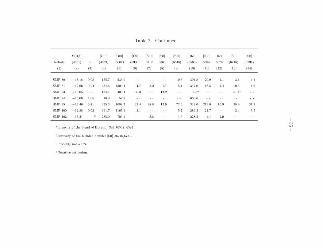
In Table 2 we report the measured line intensities. Column (1) gives the common

3IRAF is distributed by the National Optical Astronomy Observatory, which is oper-

ated by the Association of Universities for Research in astronomy, Inc., under cooperative

agreement with the National Science Foundation.

– 8 –

names, Column (2) gives the logarithmic Hβ intensities, not corrected for extinction, in erg

cm−2 s−1; column (3) lists the logarithmic optical extinction at Hβ ; columns (4) to (14)

give the line intensities for each nebula, relative to Hβ =100, not corrected for extinction.

The line identifications, which are given in the column headings, were unambiguous in spite

of the lack of a wavelength comparison arc since only the most prominent nebular lines are

detectable in the spectrograms.

2.3. Two-dimensional spectral extraction

The geometric calibration of the 2D spectra is performed with the STIS calibration

pipeline module x2d, which produces a rectified 2D spectrum which is linear in both the

wavelength and the spatial directions. The output spectrum has units of [ergs cm−2 s−1

A −1 arcsec−2]. We used the 2D spectra to measure the 2D line intensity of all detected

spectral lines, using the same extraction windows and background offsets as the 1D spectral

extraction (see Tab. 1), so the two measurements are readily comparable, and they offer a

check on the procedure and on the calibrated image quality.

Two of the angularly largest of our targets, SMP 93 and SMP 59, suffered from severe

overlap of the emission lines. For these nebulae it was essential to apply a deblending

technique on the 2D spectral images in order to separate the monochromatic images in the

Hα-[N II] group. We used the following simple procedure:

1. The images were sky-subtracted by using the mean signal within a suitable sky

window (see Table 1 for the center and sizes of the extraction windows).

2. We take advantage of the fact that the [N II] lines are identical in shape and have a

fixed intensity ratio. This allows us to use the redward, uncontaminated portion of

λ6584 line to subtract from the blend at the position of the λ6548 line; likewise the

– 9 –

uncontaminated blueward portion of the [N II] λ6548 line was used to subtract from

the blend at the position of the λ6584 line, leaving an uncontaminated Hα image.

3. We obtain the uncontaminated [Nii] image by subtracting the reconstructed Hα image

from the entangled image group.

A check on the quality of the above procedure has been performed by comparing the

total flux of the Hα plus [N II] blend with the sum of the flux from the blend as measured

with the 1-D technique. The agreement is good at least to the 10% level in the PNs

analyzed in this paper. However, it is clear that the technique is far from perfect: the

relative intensities for Hα for both SMP 93 and SMP 59 is much less than what is possible

for a nebular gas. Our technique undoubtedly fails to assign the correct total flux in these

line, and we report only the sum of the Hα and [Nii] intensities in Table 2. Furthermore,

data relative to these two PNs will not be entered in the diagnostic plots of this paper,

wherever the extinction corrected fluxes are used.

Fow SMP 59 and SMP 93, the [Sii] λ6716-6731 lines are also superimposed in the

dispersion direction. In this case, since the line ratio is not known (it depends on the

electron density) we measure the line blend, and give it in Table 2.

2.4. Error analysis

The 1D and 2D intensities can be compared to make a detailed analysis of the errors

in our measurements. The intensities for a given emission line and nebula should be

the same no matter the method used for the analysis. On the other hand, we should

limit this comparison to the nebulae whose images do not overlap in the dispersion

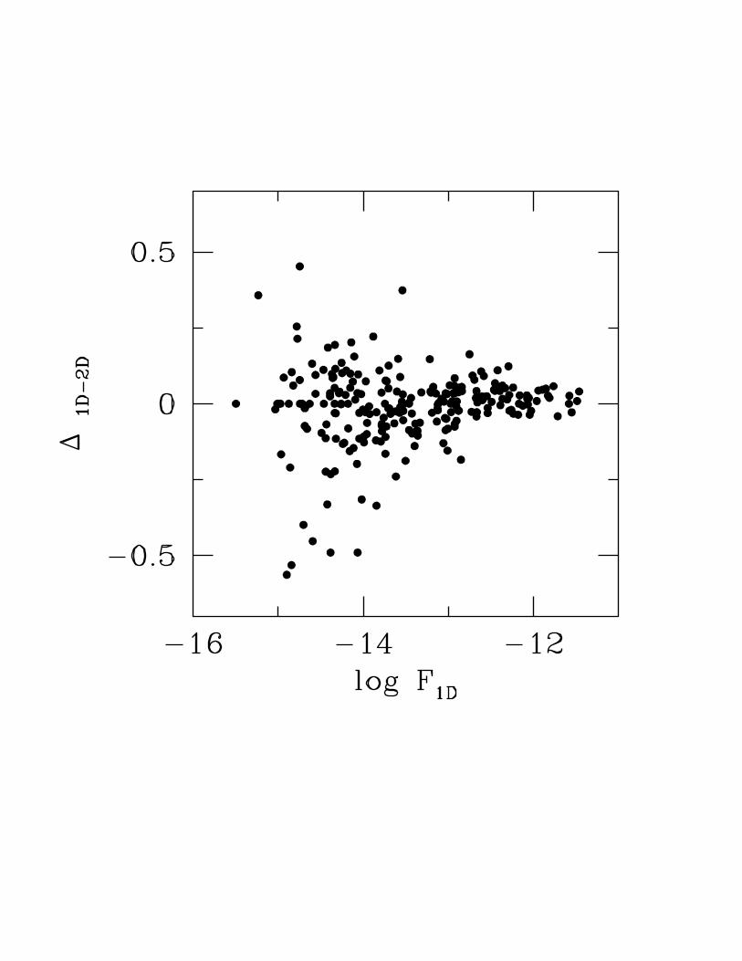
direction. We calculate the normalized difference between 1D and 2D measurements as

∆1D−2D = (F1D − F2D)/F1D for each spectral line and each PN in our sample. We plot

– 10 –

∆1D−2D against the 1D flux in Figure 1. We find that the difference depends strongly on

the observed line intensity. In particular: |∆1D−2D| < .05 if logF > −12.25, |∆1D−2D| < .15

if −12.25 < logF < −12.75, |∆1D−2D| < .2 if −12.75 < logF < −13.5, |∆1D−2D| < .25 if

−13.5 < logF < −14.5, and finally |∆1D−2D| < .55 if logF > −14.5. The only exception

to these results are a handful of data points in the −13.5 < logF < −14.5 interval. These

are the [N II] λ6584 lines that may be blended with the Hα lines, even for relatively small

objects (e. g., SMP 10 and SMP 100), and another couple of lines whose measurements

have very high errors (the [O I] λ6363 line in SMP 78 and SMP 9, and the He I λ6678 line

in SMP 81).

We have also examined the variance of ∆1D−2D with respect to the nebular radii, to

find that there is no dependence of the error in the flux measurements to the size of the

nebula, nor on the morphological type. We conclude that the errors listed above, in relation

to the intensity of the 1D spectral lines, are the formal internal observational errors for the

fluxes presented in this paper.

In order to asses the quality of our data, and the improvement over the published

line intensities, we have compared the measured MC PN intensity ratios of Table 2 to

the fluxes published by Vassiliadis et al. (1992), Meatheringham & Dopita (1991a), and

Meatheringham & Dopita (1991b). In all, we found published fluxes for 15 of 29 planetaries.

The line intensities from Meatheringham & Dopita (1991a) and Meatheringham & Dopita

(1991b) are corrected for extinction, so it was necessary to apply the reddening function

before comparing them to our data. To this end, we use the extinction constants given

by the individual references, and average Galactic reddening curve of Savage & Mathis

(1979), which is reliable at these wavelengths even for the LMC (Howarth 1983). In Figure

2 we show the comparison between our line intensity ratios and those from the references

above. The intensity ratios are plotted in logarithmic form, to allow the simultaneous view

– 11 –

of low and high fluxes. The correspondence of our intensities to the ones in the literature is

generally good, and typically within the observing errors quoted in the references (indicated

with vertical lines on the plot). The notable exceptions are the [N II] 6548 lines of SMP 10

and SMP 100, overestimated in the references (the dots in the middle of Fig. 2). We believe

that our [N II] measurements for these two nebulae are more reliable than those by the

literature source (Vassiliadis et al. 1992). In fact, we know that the [N II] 6584/6548 ratio

should be approximately 3 (Osterbrock 1989), and our ratios are 2.96 and 2.98 respectively

for SMP 10 and SMP 100, while the ratios from Vassiliadis et al. (1992) are 11.4 and 11.1

respectively. The errors in the reference may be caused by the poor separation of the

[N II] and Hα lines in the dispersion direction. Vassiliadis et al. (1992), for example, use a

bandpass of FWHM 16 A to observe the Hα lines, and this separation may be not enough

for SMP 10 and SMP 100, where the [N II] lines have low intensity.

A close inspection of Figure 2 reveals a small discrepancy in the [O III] λλ4959, 5007

line intensities (the clump of dots at log F ≈ 2.5). The source of the mismatch may lie

in a difference in the Hβ fluxes, which are used to scale the intensities and which are

often weakly exposed in our spectrograms for larger nebulae. The ultimate cause of the

discrepancy may lie with a systematic problem in the flux calibration for the STIS CCD.

Stys & Walborn (2001) found that an apparent degradation in the sensitivity of the STIS

CCD with time (which is not yet corrected in the calibration pipeline) may in fact have

its root cause in a degradation of the CCD charge transfer efficiency. While not yet well

characterized for the grating/central wavelength combinations used here, in general the

effect is that charge lost during the CCD readout is manifested as lower measured fluxes.

Depending upon the brightness of the surrounding mean sky and the number of detected

counts per pixel of the emission feature, the effect could range from less than a percent to

as much as 15% (Stys & Walborn 2001) for the emission lines reported here. We anticipate

that the effect for the Hβ fluxes (and hence the scaling for all of the emission lines) for

– 12 –

angularly large nebulae is likely in the range of 1–3%. The effect on the very weakest lines

(such as [O I]) in large nebulae may approach 10%, but the effect on well exposed lines in

small nebulae is likely negligible.

3. Results

3.1. Nebular morphology in various lines

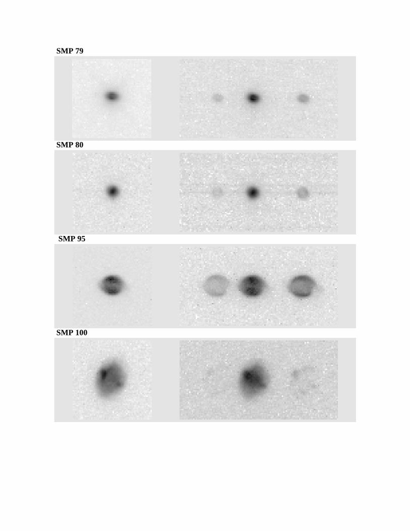
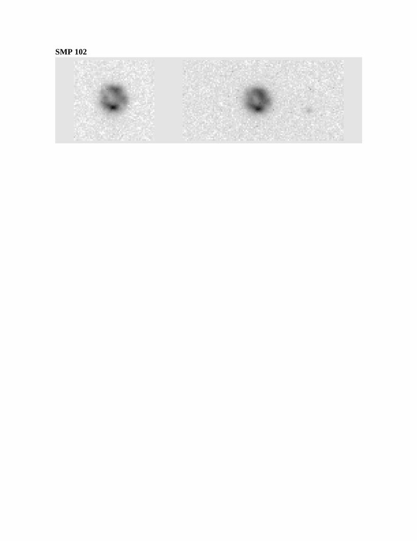
The calibrated slitless images of all but the very largest LMC PNs are shown in Figure

3. For each nebula we show the [Oiii] 5007 A section of the G430M spectra, when available,

and the Hα and [Nii] line group section of the G750M spectra. The images of SMP 94

are not shown in Figure 3, because we are convinced this object is not a PN, based on its

spectral structure (see Paper I). The slitless images for the two largest nebulae are shown

in Figure 4, where we show the [Oiii] 5007 A images, the Hα and [Nii] group, and the

[Nii] images as reconstructed with the algorithm described in §2.3.

Paper I describes the morphology of our sample nebulae in detail. In the following

we limit the description to interesting morphological features of the spectra that have not

been mentioned in Paper I. Morphological types are taken from Paper I unless stated

otherwise. As in the other papers of this series, we use the Manchado et al. (1996a)

morphological classification scheme, and we also add the bipolar core class. Hereafter, when

we refer to symmetric PNs we include E and R without a detected bipolar core, and with

asymmetric PNs we indicate the bipolar and quadrupolar (B), and the bipolar core (Rbc

and Ebc) PNs. We keep pointsymmetric PNs outside these groups.

• J 41: The nebular morphology is Ebc. It is observed only with the G750M

configuration, and only the Hα emission is detected. No low-ionization structures

(hereafter “LIS”’) are seen in this object.

– 13 –

• SMP 4: The nebular morphology is E. This attached halo multiple shell PN shows

its morphology in all the detected lines. This is shown for [Oiii] λ5007 A and Hα in

Figure 3, and it is also true for Hβ and [Oiii] λ5007 A. The emission in the [Nii] lines

was marginally detected below the 3σ level. No LIS’ are seen in this object.

• SMP 9: The nebular morphology is Ebc. The barrel shape is shown in all detected

emission lines, including [Nii] . No LIS’ are seen.

• SMP 10: The nebular morphology is P. The [Nii] emission occurs only in the arms of

this PN. There are three distinct morphological features: an inner ellipse (not visible

in [Nii] ), a round edge-brightened mantle that surrounds it, and two “spiral arms”

that are most prominent in [Nii] . We note that the enhanced emission that defines

the inner ellipse is oriented such that the major axis is aligned with the arm structure

in the outer nebula. It is conceivable that this feature traces more subtle, unresolved

structure such as a jet from the central star that terminates at the ends of the arms,

similar to the Cat’s Eye nebula (NGC 6543). Note that the photometric radius

measured by Shaw et al. (2001) on the [Oiii] image is very close to a photometric

radius measured on the [Nii] image. Although this nebula is rather extended, none of

2D the spectral lines overlap.

• SMP 13: The nebular morphology is Rbc. The same patchy morphology is visible in

all detected lines. The [Nii] emission (see Fig. 3) is very faint except along the lobe

edges where its structure is clumpy. This behavior is characteristic of Galactic bipolar

PNs such as NGC 2346 and NGC 6537, which are similar in appearance to SMP 13.

In the spectral data we can see a faint stellar spectrum that could be associated with

the central star.

• SMP 16: The nebular morphology is B. This very prominent bipolar shows its

morphology in all detected lines. As mentioned in Paper I, the [Nii] emission reveals

– 14 –

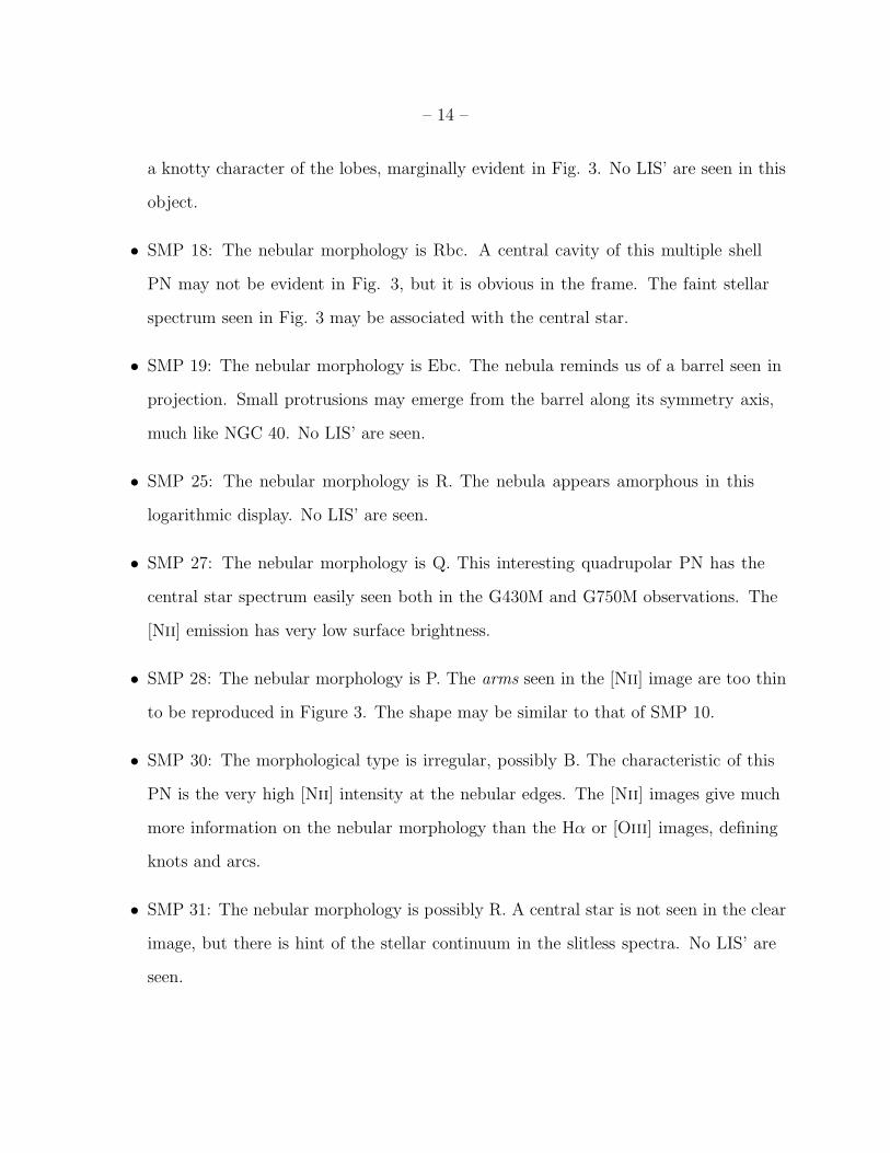
a knotty character of the lobes, marginally evident in Fig. 3. No LIS’ are seen in this

object.

• SMP 18: The nebular morphology is Rbc. A central cavity of this multiple shell

PN may not be evident in Fig. 3, but it is obvious in the frame. The faint stellar

spectrum seen in Fig. 3 may be associated with the central star.

• SMP 19: The nebular morphology is Ebc. The nebula reminds us of a barrel seen in

projection. Small protrusions may emerge from the barrel along its symmetry axis,

much like NGC 40. No LIS’ are seen.

• SMP 25: The nebular morphology is R. The nebula appears amorphous in this

logarithmic display. No LIS’ are seen.

• SMP 27: The nebular morphology is Q. This interesting quadrupolar PN has the

central star spectrum easily seen both in the G430M and G750M observations. The

[Nii] emission has very low surface brightness.

• SMP 28: The nebular morphology is P. The arms seen in the [Nii] image are too thin

to be reproduced in Figure 3. The shape may be similar to that of SMP 10.

• SMP 30: The morphological type is irregular, possibly B. The characteristic of this

PN is the very high [Nii] intensity at the nebular edges. The [Nii] images give much

more information on the nebular morphology than the Hα or [Oiii] images, defining

knots and arcs.

• SMP 31: The nebular morphology is possibly R. A central star is not seen in the clear

image, but there is hint of the stellar continuum in the slitless spectra. No LIS’ are

seen.

– 15 –

• SMP 34: The nebular morphology is E. A different morphology is detected in the

[Nii] lines. Although these lines are faint, a hint of a bipolar shape is shown. No LIS’

are seen.

• SMP 46: The nebular morphology is Ebc. A central cavity is particularly clear in

[Nii] . No LIS’ are seen.

• SMP 53: The nebular morphology is E, possibly Ebc. A ringlike structure is clearly

seen in the [Nii] emission lines. Filamentary LIS’ surround the core, something like

SMP 30.

• SMP 58: The nebular morphology may be R. A barely resolved PN, the central star

spectrum is seen in the G750M slitless observations (see Fig. 3). An emission feature

at about 6577A is probably stellar. No LIS’ are seen.

• SMP 59: The nebular morphology is probably Q. A spectacular PN, its morphology

is particularly evident in the [Nii] emission lines. The reconstructed [Nii] image in

Fig. 4 shows that there may be multiple emission or knots in this nebula.

• SMP 65: The nebular morphology is R. No LIS’ are seen.

• SMP 71: The nebular morphology is E. No LIS’ are seen.

• SMP 78: The nebular morphology is Ebc. No LIS’ are seen.

• SMP 79: The nebular morphology is Ebc. Ringlike structures are evident in the

[Nii] emission. No LIS’ are seen.

• SMP 80: The nebular morphology is R. Ringlike structures are evident in the

[Nii] emission, and the central star spectrum is seen in the slitless observations with

the G750M grism.

– 16 –

• SMP 81 is not shown in Figure 3 for lack of interesting extended features. The

nebular morphology is probably R. An extremely faint, marginally detected central

star spectrum is seen in the G750M slitless observations.

• SMP 93: The nebular morphology is B. The best way to study the morphology of

this spectacular bipolar PN is to look at the [Nii] reconstructed image of Fig. 4.

The central ring and the lobes are enhanced at this wavelength. The morphology

of the Hα emission looks similar to that of the [Oiii] emission. The edges of the

main morphological structures are low in emission, much like most Galactic PNs.

NGC 6445 is similar in structure to SMP 93.

• SMP 94: The nebular morphology is unresolved. We believe that this object is not a

PN (see the discussion in Paper I). Although we include the line flux analysis in Table

2 for SMP 94, we do not include it in the Figures, not in the following analysis and

related plots.

• SMP 95: The nebular morphology is Ebc. Faint low-ionization ansae can be seen in

[Nii] .

• SMP 100: The nebular morphology is Ebc, or Q. The [Nii] emission lines show the

knots’ outline of this interesting PN. No LIS’ are seen.

• SMP 102: The nebular morphology is R, possibly bc. The interior shows a round

clumpy ring. The brightest of the knots is faintly visible in [Nii] .

From the above analysis we note that, while the morphological type is more or less the

same in all detected lines for most PN, the morphologies are sometimes more evident in the

low-ionization images, as if these arise primarily along the nebular border. Some distinct,

compact emission features are seen most prominently in [Nii] .

– 17 –

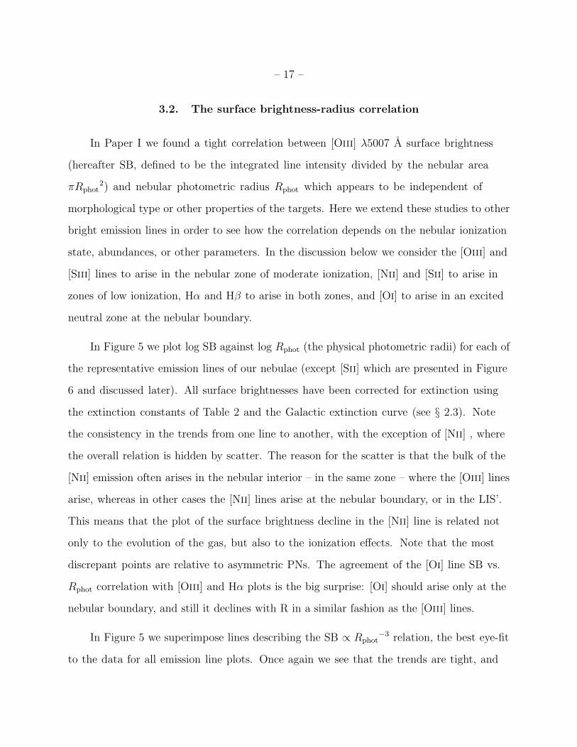
3.2. The surface brightness-radius correlation

In Paper I we found a tight correlation between [Oiii] λ5007 A surface brightness

(hereafter SB, defined to be the integrated line intensity divided by the nebular area

πRphot2) and nebular photometric radius Rphot which appears to be independent of

morphological type or other properties of the targets. Here we extend these studies to other

bright emission lines in order to see how the correlation depends on the nebular ionization

state, abundances, or other parameters. In the discussion below we consider the [Oiii] and

[Siii] lines to arise in the nebular zone of moderate ionization, [Nii] and [Sii] to arise in

zones of low ionization, Hα and Hβ to arise in both zones, and [Oi] to arise in an excited

neutral zone at the nebular boundary.

In Figure 5 we plot log SB against log Rphot (the physical photometric radii) for each of

the representative emission lines of our nebulae (except [Sii] which are presented in Figure

6 and discussed later). All surface brightnesses have been corrected for extinction using

the extinction constants of Table 2 and the Galactic extinction curve (see § 2.3). Note

the consistency in the trends from one line to another, with the exception of [Nii] , where

the overall relation is hidden by scatter. The reason for the scatter is that the bulk of the

[Nii] emission often arises in the nebular interior – in the same zone – where the [Oiii] lines

arise, whereas in other cases the [Nii] lines arise at the nebular boundary, or in the LIS’.

This means that the plot of the surface brightness decline in the [Nii] line is related not

only to the evolution of the gas, but also to the ionization effects. Note that the most

discrepant points are relative to asymmetric PNs. The agreement of the [Oi] line SB vs.

Rphot correlation with [Oiii] and Hα plots is the big surprise: [Oi] should arise only at the

nebular boundary, and still it declines with R in a similar fashion as the [Oiii] lines.

In Figure 5 we superimpose lines describing the SB ∝ Rphot−3 relation, the best eye-fit

to the data for all emission line plots. Once again we see that the trends are tight, and

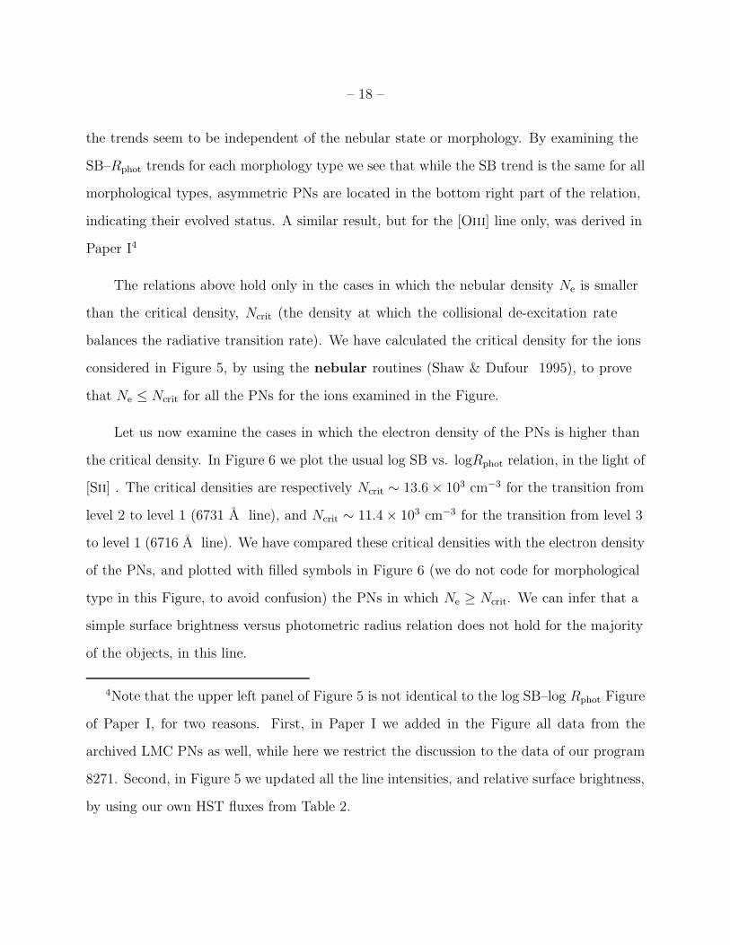
– 18 –

the trends seem to be independent of the nebular state or morphology. By examining the

SB–Rphot trends for each morphology type we see that while the SB trend is the same for all

morphological types, asymmetric PNs are located in the bottom right part of the relation,

indicating their evolved status. A similar result, but for the [Oiii] line only, was derived in

Paper I4

The relations above hold only in the cases in which the nebular density Ne is smaller

than the critical density, Ncrit (the density at which the collisional de-excitation rate

balances the radiative transition rate). We have calculated the critical density for the ions

considered in Figure 5, by using the nebular routines (Shaw & Dufour 1995), to prove

that Ne ≤ Ncrit for all the PNs for the ions examined in the Figure.

Let us now examine the cases in which the electron density of the PNs is higher than

the critical density. In Figure 6 we plot the usual log SB vs. logRphot relation, in the light of

[Sii] . The critical densities are respectively Ncrit ∼ 13.6× 103 cm−3 for the transition from

level 2 to level 1 (6731 A line), and Ncrit ∼ 11.4× 103 cm−3 for the transition from level 3

to level 1 (6716 A line). We have compared these critical densities with the electron density

of the PNs, and plotted with filled symbols in Figure 6 (we do not code for morphological

type in this Figure, to avoid confusion) the PNs in which Ne ≥ Ncrit. We can infer that a

simple surface brightness versus photometric radius relation does not hold for the majority

of the objects, in this line.

4Note that the upper left panel of Figure 5 is not identical to the log SB–log Rphot Figure

of Paper I, for two reasons. First, in Paper I we added in the Figure all data from the

archived LMC PNs as well, while here we restrict the discussion to the data of our program

8271. Second, in Figure 5 we updated all the line intensities, and relative surface brightness,

by using our own HST fluxes from Table 2.

– 19 –

On the other hand, most nebulae are less dense than the critical density for the

[Sii] λ6716A line, and a sizable fraction of them are less dense than the critical density for

the [Sii] λ6731A line. This effect explains the different relation observed.

3.3. Electron density and ionized masses

Nebular densities Ne of the 12 MC PNs with the brightest [Sii] lines were estimated

using the IRAF package nebular and assuming an electron temperature of 104 K. The

electron densities calculated in this way are reliable only for the density interval between

300 and 7000 cm−3 (Stanghellini & Kaler 1989). The log Ne – log Rphot is shown in Figure

7. Morphological types are plotted with different symbols. Based on a small and selected

sample, the densities of MC PNs are not related to their morphologies.

If all PNs have the same mass, morphology, expansion rate, and density boundedness

(i.e., ultraviolet opacity) then we would expect a tight negative correlation between density

and radius. We see only a loose correlation, if any at all. This is no surprise. The same

absence of a tight density–radius correlation was seen earlier by Dopita & Meatheringham

(1990) based on ground-based data.

The ionized masses have been calculated from the [Sii] densities and the photometric

radii using the methodology of Boffi & Stanghellini (1994). This method assumes spherical

geometry and uniform density within the filled parts of the nebula, which is obviously the

exception and not the rule (Figs. 3 and 4), but does not assume a value for the filling factor

(ǫ) of the nebulae (Boffi & Stanghellini 1994). Implicit also is the assumption that the

[Sii] densities are characteristic of the entire nebula, whereas we have seen that knotty and

filamentary LIS’ sometimes dominate the [Nii] and [Sii] emission.

We find that the average ionized mass is 0.21 M⊙, the same that has been found

– 20 –

by Boffi & Stanghellini (1994) from a larger LMC PN sample, albeit without diameters

measured directly from deep HST images. The ionized masses for the only bipolar and

elliptical PNs in our sample with reliable electron density are respectively 0.33 M⊙and

0.17 M⊙. Barlow (1987) used the [Oii] electron density to derive the ionized mass of 32

Magellanic Cloud PNs, and they found an average mass of 0.25 ± 0.17 M⊙for the complete

sample, and 0.39 ± 0.22 M⊙for the type I PNs within their sample. Our results are thus

in agreement with those of Barlow (1987), including a possible ionized mass offset between

PN types, type I PNs and bipolar PNs being the more massive ones. A much larger data

set is needed to confirm these trends.

The ionized mass versus radius logarithmic relation is plotted in Figure 8 using the

same symbol definitions as in Figure 7. The tight correlation found for Galactic PNs (Boffi

& Stanghellini 1994) is not found in this plot of LMC PNs, where the two (logarithmic)

variables have a low correlation coefficient of 0.35. Much of this scatter is the result of

inappropriate assumptions such as spherical symmetry, constant density, and accurate

nebular radii. The assignment of a nebular radius is especially treacherous for bipolar PNs

with open, slowly fading lobes along the major axis and bright, sharp and closely spaced

edges along the minor axis.

3.4. Nebular excitation

In planetary nebulae, one measure of stellar evolutionary state is nebular excitation,

which tracks the evolution of the temperature of the central star. For ionization bounded

nebulae this can be gauged from the relative volumes of regions dominated by He◦, He+

and He++. Nebular excitation is best measured using ratios of recombination lines of H and

He which are only slightly affected by electron temperature Te. The signal-to-noise and

restricted bandwidths of our spectra render this impractical.

– 21 –

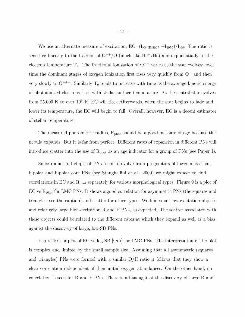
We use an alternate measure of excitation, EC=(I[O III]5007 +I4959)/IHβ. The ratio is

sensitive linearly to the fraction of O++/O (much like He+/He) and exponentially to the

electron temperature Te. The fractional ionization of O++ varies as the star evolves: over

time the dominant stages of oxygen ionization first rises very quickly from O+ and then

very slowly to O+++. Similarly Te tends to increase with time as the average kinetic energy

of photoionized electrons rises with stellar surface temperature. As the central star evolves

from 25,000 K to over 105 K, EC will rise. Afterwards, when the star begins to fade and

lower its temperature, the EC will begin to fall. Overall, however, EC is a decent estimator

of stellar temperature.

The measured photometric radius, Rphot should be a good measure of age because the

nebula expands. But it is far from perfect. Different rates of expansion in different PNs will

introduce scatter into the use of Rphot as an age indicator for a group of PNs (see Paper I).

Since round and elliptical PNs seem to evolve from progenitors of lower mass than

bipolar and bipolar core PNs (see Stanghellini et al. 2000) we might expect to find

correlations in EC and Rphot separately for various morphological types. Figure 9 is a plot of

EC vs Rphot for LMC PNs. It shows a good correlation for asymmetric PNs (the squares and

triangles, see the caption) and scatter for other types. We find small low-excitation objects

and relatively large high-excitation R and E PNs, as expected. The scatter associated with

these objects could be related to the different rates at which they expand as well as a bias

against the discovery of large, low-SB PNs.

Figure 10 is a plot of EC vs log SB [Oiii] for LMC PNs. The interpretation of the plot

is complex and limited by the small sample size. Assuming that all asymmetric (squares

and triangles) PNs were formed with a similar O/H ratio it follows that they show a

clear correlation independent of their initial oxygen abundances. On the other hand, no

correlation is seen for R and E PNs. There is a bias against the discovery of large R and

– 22 –

E PNs owing to their very low surface brightnesses. But most of all we believe that the

fraction of escaping ultraviolet radiation increases drastically for R and E PNs. Variations

in mass or expansion speed will tend to introduce scatter into SB for a group of PNs.

The Hα recombination-line luminosity of an expanding PN is a measure of the rate

at which ionizing photons are being absorbed in the nebula. We expect the Hα flux to

be constant while the nebula is ionization bounded and to drop thereafter until the star

itself drops in UV photon emission rates late in its life. In Figure 11 we plot the Hα line

luminosity, corrected for extinction, against EC. Since all PNs in this plot are at the same

distance, the Hα intensity is proportional to the stellar luminosity. Note that in Figure

11 the excitation constant increases from right to left in the plot, as does the effective

temperature in the HR diagram.

Dopita & Meatheringham (1990) have used a similar diagram to compare the observed

LMC and SMC PNs with simple evolutionary models. The novelty of our approach is

that we added the information on nebular morphology. In Figure 11 we can follow the PN

evolution in two dimensions, exactly as we follow the stellar evolution in the HR diagram.

We can see the simultaneous effects of changes in the effective temperature (through the

parameter EC) and of the luminosity (through the Hα brightness) for different nebular

morphologies. PNs evolve first from right to left (and from bottom to top) as their central

stars get hotter and their shells get thinner, then from top left to bottom right as the

central stars evolve in the cooling line, at constant radii.

Naturally, much modeling is needed before we could derive a quantitative conclusion

from Figure 11, but we feel that the empirical result is very strong, that is, most of

the observations of asymmetric PNs in the LMC are consistent with them being on the

cooling sequence, beyond the central star’s temperature maxima. The opposite is true for

symmetric PNs. This observational result is consistent with our other findings that relate

– 23 –

asymmetry with higher progenitor mass, in this case it looks like also the post-AGB stellar

mass is higher for asymmetric PNs. Our future study on the central star’s photometry will

clarify some of the open questions posed by these diagrams, and appropriate hydrodynamic

modeling will complete the description of the evolution of PN in the LMC.

3.5. Nebular extinction

We analyzed the extinction in this sample of nebulae to look for evidence of internal

dust, and for any variations with morphological type. Ciardullo & Jacoby (1999) reported

evidence of a correlation of extinction with the mass of the central star for PNs in the

Magellanic Clouds and in M31. We examined some nebulae in our sample to look for

spatial variations in the extinction, which we believe would be a strong indicator of the

presence of dust internal to the nebulae. We took ratios of the Hβ and Hα images for

PNs where the extinction constant was relatively high, or that had morphological features

that can be associated with the presence of internal dust, such as the pinched waist of the

bipolar nebulae SMP 16 and SMP 30. In no case did we find significant spatial variations

in Hβ/Hα, at least on spatial scales of ∼ 0.04 pc. We note, however, that many of the PNs

with high extinction are angularly small, and furthermore the S/N ratio of our Hβ images

is often not high. Still, for nebulae within our sample that lend themselves to this analysis,

the internal extinction, where present, must be spatially uniform on small spatial scales.

Another way to address the question of whether the extinction is internal to the

nebulae is to examine whether it declines with nebular physical radius, as might be expected

if internal dust were either destroyed or geometrically diluted as the nebula expands. We

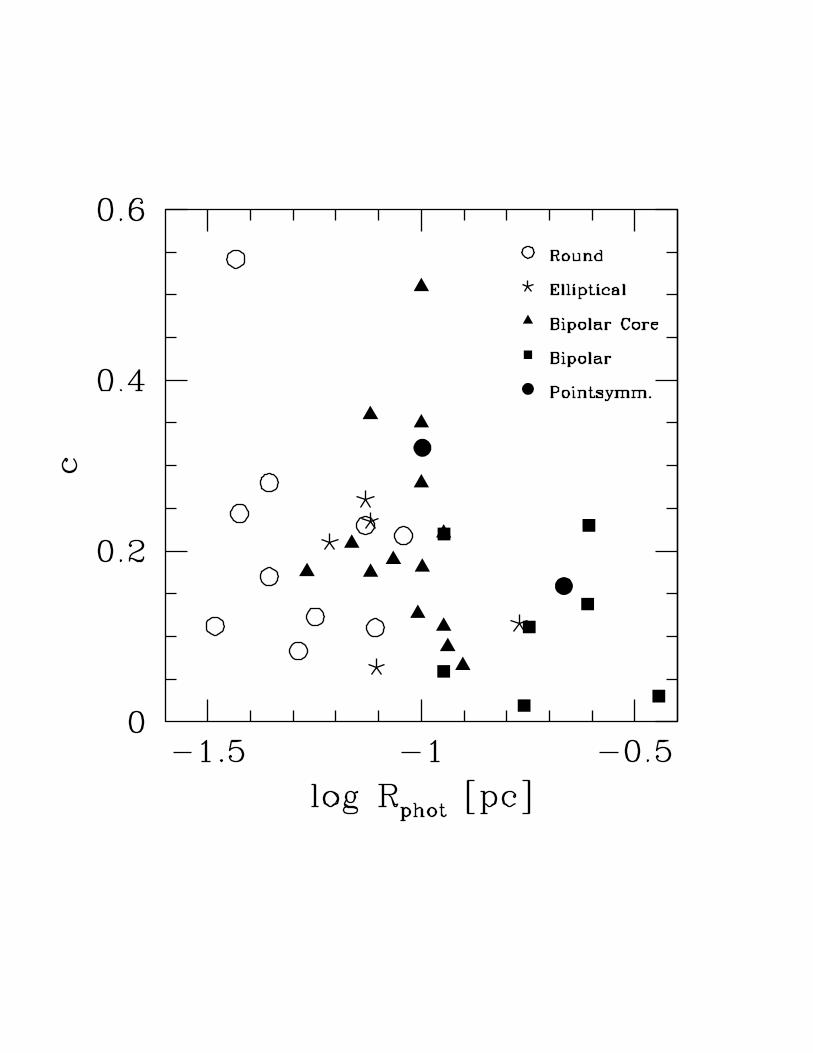
plot in Figure 12 the nebular extinction constant vs. the log of the physical radius for all

nebulae in this sample, and we also include the PNs in the archived sample by Dopita

(HST program 6407, see also Paper I). The Figure shows that the amount of extinction

– 24 –

does not depend on morphological type, except possibly for large bipolar nebulae where c is

generally low. It also shows that the amount of extinction depends only weakly on physical

size, in that nebulae smaller than 0.1 pc suffer at least some extinction. This question

should be examined again with a larger data set, but for now the safest conclusion is that

the extinction for PNs in this sample spans a large range at all sizes and does not depend

strongly, if at all, on morphological type. Stanghellini, et al. (2000) showed for Large

Magellanic Cloud PNs that bipolar (and bipolar-core) morphology correlates with chemical

properties that are related to higher-mass central stars. Yet the absence here of any relation

between bipolar morphology and extinction, and the lack of internal variation in extinction

on modest spatial scales, suggests that there is no clear relationship between internal

nebular extinction and central star mass. The lack of nebulae smaller than 0.1 pc with zero

extinction may indicate the presence of dust within these nebulae; our spatial resolution is

insufficient to search for spatial variations in extinction. It would be worthwhile to observe

these nebulae in the thermal infrared to examine the dust properties more thoroughly. In

any case, we find no evidence that internal extinction in LMC PNs varies with central star

core mass.

4. Discussion

In this paper we have shown the STIS slitless observation of a group of 29 LMC PNs,

and analyzed the spectroscopic data. The images of Figures 3 and 4 present an unique data

set that includes a wealth of morphological and spectral information. The line intensities

measured from the slitless spectra, although limited to the brightest spectral lines in the

observed wavelength windows, represent some of the best quality spectral data for the

LMC PNs. By adding spatial information to the spectrograms, we are able to determine an

accurate morphology, where the effects of the ionization structure are fully understood. Our

– 25 –

comparison of the 1D to the 2D line fluxes helps us to characterize our internal consistency,

while the comparison to published data reveals the high photometric quality of these data

The nebular emission at the different wavelengths has been analyzed in various ways.

We obtain the following results.

1. While the Hα and [Oiii] lines are perfect for morphological studies of the main

body of the PNs, the [Nii] emission lines are ideal to detect knots, ansae, and other

deviation from symmetry, not always detectable in the Hα light, and to clarify the

morphological classification.

2. The surface brightness relation with the photometric nebular radius is indistinguishible

for all the observed lines where the nebular electron density is smaller than the critical

density, and with the exception of the [Nii] lines. The very tight, universal log SB

∝ -3 Rphot relation indicates the nebular evolution. Such a relation could be used to

calibrate the Galactic PN distance scale.

3. The marginal correlations between the photometric radii and the electron densities

and the ionized nebular masses indicate that the spherical approximation is wrong for

the LMC PNs, and that assuming that all PNs have the same ionized mass is very

misleading. We found that the average ionized mass for our sample is 0.21 M⊙. A

marginal correlation between asymmetry and high ionized mass was detected.

4. The [Oiii] to Hβ line ratio is a good measure of the nebular excitation. We find

that there is a tight correlation between EC and size in asymmetric PNs, suggesting

that these nebulae are on a faster evolving track. This result is in agreement with

our previous results of Paper I, and Stanghellini, et al. (2000), that observations of

asymmetric LMC PNs are in accord with a rapidly evolving, more massive progenitor,

younger generation planetary nebula sequence, compared to the low mass, slow

– 26 –

evolving, round PNs.

5. The internal extinction of the observed nebulae is generally low, and does not depend

markedly on morphological type. We find no evidence for a relation between the

progenitor mass indicators and the extinction of the nebulae.

In the future, we plan to extend this analysis to our other data samples, the SMC PNs that

have been observed in Cycle 9, and an expanded LMC data set that is being collected at

the time of writing. At the same time, for the dataset presented in this paper, we will also

extract the information about the central stars of those PNs. Eventually we will relate the

stellar and nebular properties of all the samples in study.

While most of the results presented in this paper (especially from points 2 and 4 above)

need extensive nebular modeling to be understood, their empirical value is nonetheless

remarkable. We confirm, with this work, the importance of slitless spectroscopy for

maximizing the rate of useful information of these objects. Our future plans include

hydrodynamical modeling of the SB vs. Rphot relation to test its physical meaning, and to

asses its validity as a tool to build the LMC based PN distance scale. We have much to

understand about the shape and universality of this relationship which may be useful for

PN distances as the period-luminosity relationship for Cepheid variable stars.

Our Web page, http://archive.stsci.edu/hst/mcpn/, includes many of the published

data and data analysis, and it is a part of the Hubble Data Archive.

This work was supported by NASA through grant GO-08271.01-97A from Space

Telescope Science Institute, which is operated by the Association of Universities for

Research in Astronomy, Incorporated, under NASA contract NAS -26555. We thank an

anonymous referee for an essential suggestion.

– 27 –

Fig. 1.— Comparison of the 1D to the 2D line intensity measurement from our HST data.

We plot ∆1D−2D against the logarithmic 1D flux for all nebulae of our sample and for all

available lines. We do not plot data for those nebulae whose lines overlap in the dispersion

direction, see text.

Fig. 2.— Comparison of the measured line intensity ratios with those in the literature, in

logarithmic scale. The vertical lines represent the minimum errorbars for the reference fluxes.

Fig. 3.— [Oiii] ,Hα , and [Nii] images of the program nebulae (all PNs except SMP 59 and

SMP 93).

Fig. 4.— [Oiii] ,Hα , and [Nii] images of SMP 59 and SMP 93.

Fig. 5.— Surface brightness decline for the mutliwavelength images of the PNs in our STIS

survey. Emission lines for which the SB is derived are indicated in the panels. Symbols

indicate morphological types: open circles= round, filled circles= pointsymmetric, stars=

elliptical, filled triangles=bipolar core, filled squares= bipolar (and quadrupolar) planetary

nebulae. The photometric radii are measured from the [Oiii] λ5007 A images (see text).

Fig. 6.— The log SB vs. log Rphot relation for the [Sii] lines. Filled symbols: PNs with

Ne ≥ Ncrit, for [Sii] 6716 A (left panel) and [Sii] 6731 A (right panel). Points are not coded

for morphology, to avoid confusion.

Fig. 7.— Logarithmic electron density from the [Sii] doublet vs. log Rphot.

Fig. 8.— Logarithmic ionized mass vs. log Rphot.

Fig. 9.— Excitation constant, as defined in the text, plotted against the logarithmic photo-

metric radius.

Fig. 10.— Logarithmic [Oiii] surface brightness vs. excitation constant.

– 28 –

Fig. 11.— Logarithmic Hα line intensity vs. excitation constant.

Fig. 12.— Logarithmic extinction at Hβ λ4861 vs. log Rphot.

– 29 –

REFERENCES

Balick, B. 1987, AJ, 94, 671

Barlow, M. J. 1987, MNRAS, 227, 161.

Boffi, F. R., & Stanghellini, L. 1994, A&A, 284, 248

Ciardullo, R., & Jacoby, G. H. 1999, ApJ, 515, 191

Dopita, M. A., & Meatheringham, S. J. 1990, ApJ, 357, 140

Meatheringham, S. J., & Dopita, M. A. 1991a, ApJS, 75, 407

Meatheringham, S. J., & Dopita, M. A. 1991b, ApJS, 76, 1085

Frank, A. 2000, ASP Conf. Ser. 199: Asymmetrical Planetary Nebulae II: From Origins to

Microstructures, 225

Icke, V., Preston, H. L., & Balick, B. 1989, AJ, 97, 462

Howarth, I. D. 1983, MNRAS, 203, 301

Leitherer, C., & Bohlin, R. C. 1997, STIS Instrument Science Report 97–13 (Baltimore:

ST ScI)

Leitherer, C., et al. 2000, STIS Instrument Handbook, Version 4.0 (Baltimore: ST ScI)

McGrath, M. A., Busko, I., & Hodge, P. E. 1999, STIS Instrument Science Report 99–03

(Baltimore: ST ScI)

Manchado, A., Guerrero, M., Stanghellini, L., & Serra-Ricart, M. 1996a, The IAC

Morphological Catalog of Northern Galactic Planetary Nebulae (Tenerife: Instituto

de Astrofısica de Canarias)

– 30 –

Manchado, A., Stanghellini, L., & Guerrero, M. A. 1996b, ApJ, 466, L95

Manchado, A., Villaver, E., Stanghellini, L., & Guerrero, M. A. 2000, ASP Conf. Ser. 199:

Asymmetrical Planetary Nebulae II: From Origins to Microstructures, 17

Osterbrock, D. E. 1989, Astrophysics of Gaseous Nebulae and Active Galactic Nuclei (Mill

Valley, CA: University Science Books)

Peimbert, M. 1978, IAU Symp. 76, ed. Y. Terzian, Reidel, 215

Torres-Peimbert, S., & Peimbert, M. 1997, IAU Symp. 180, eds. H. Habing and H. Lamers,

Kluwer, 175

Savage, B., & Mathis, J. 1979, ARA&A, 17, 73

Shaw, R. A. & Dufour, R. J. 1995, PASP, 107, 896

Shaw, R. A., Stanghellini, L., Mutchler, M., Balick, B., & Blades, J. C. 2001, ApJ, 548, 727

(Paper I)

Stanghellini, L., & Kaler, J. B. 1989, ApJ, 343, 811

Stanghellini, L., Corradi, R. L. M., & Schwarz, H. E. 1993, A&A, 279, 521

Stanghellini, L., Blades, J. C., Osmer, S. J., Barlow, M. J., & Liu, X.-W. 1999, ApJ, 510,

687

Stanghellini, L., Shaw, R. A., Balick, B., & Blades, J. C. 2000, ApJ, 534, L167

Stys, D. J., & Walborn, N. R. 2001, STIS Instrument Science Report 2001–01R (Baltimore:

ST ScI)

van den Hoek, L. B., & Groenewegen, M. A. T. 1997, A&AS, 123, 305

Vassiliadis, E., Dopita, M. A., Morgan, D. H., & Bell, J. F. 1992, ApJS, 83, 87

– 31 –

This manuscript was prepared with the AAS LATEX macros v5.0.

– 32 –

Table 1. Spectrum Extraction Parameters

Ap. Center Ap. Size

Nebula Grating (pix) (pix)

(1) (2) (3) (4)

J 41 G750M 517 23

SMP 4 G430M 542 30

G750M 537 30

SMP 9 G430M 521 20

G750M 517 20

SMP 10 G430M 526 55

G750M 527 55

SMP 13 G430M 531 27

G750M 526 27

SMP 16 G430M 517 53

G750M 514 53

SMP 18 G430M 553 27

G750M 548 27

SMP 19 G430M 521 25

G750M 517 25

SMP 25 G430M 511 15

G750M 506 15

SMP 27 G430M 539 23

G750M 535 23

SMP 28 G430M 503 12

G750M 508 23

SMP 30 G430M 528 51

G750M 525 51

SMP 31 G430M 513 23

G750M 508 11

SMP 34 G430M 518 23

G750M 514 20

SMP 46 G430M 538 23

G750M 533 23

SMP 53 G430M 521 25

– 33 –

Table 1—Continued

Ap. Center Ap. Size

Nebula Grating (pix) (pix)

(1) (2) (3) (4)

G750M 516 25

SMP 58 G430M 521 23

G750M 516 23

SMP 59a G430M 521 25

G750M 516 25

SMP 65 G430M 521 25

G750M 516 25

SMP 71 G430M 521 23

G750M 516 23

SMP 78 G430M 521 23

G750M 516 23

SMP 79 G430M 521 23

G750M 516 23

SMP 80 G430M 521 15

G750M 516 15

SMP 81 G430M 521 23

G750M 516 11

SMP 93a G430M 521 25

G750M 516 25

SMP 94 G430M 521 23

G750M 516 11

SMP 95 G430M 521 27

G750M 516 27

SMP 100 G430M 521 43

G750M 516 45

SMP 102 G430M 521 29

G750M 516 29

aLarge angular size of nebula requires 2-D extrac-

tion; see text.

–34

–

Table 2. Relative Emission Line Intensities of LMC Planetary Nebulae

F (Hβ) [Oiii] [Oiii] [Oi] [Siii] [Oi] [Nii] Hα [Nii] Hei [Sii] [Sii]

Nebula (4861) c (4959) (5007) (6300) 6312 6363 (6548) (6563) 6584 6678 (6716) (6731)

(1) (2) (3) (4) (5) (6) (7) (8) (9) (10) (11) (12) (13) (14)

J 41 0.00

SMP 4 −13.55 0.12 452.6 1354.4 · · · · · · · · · · · · 312.6 · · · · · · · · · · · ·

SMP 9 −13.43 0.22 313.7 933.0 38.3 6.5 11.0 62.2 340.5 191.4 3.9 24.0 31.4

SMP 10 −13.12 0.16 377.2 1115.5 · · · · · · · · · 6.1 324.0 19.0 · · · 0.0 · · ·

SMP 13 −12.88 0.09 353.8 1068.2 4.2 1.4 1.5 7.2 306.1 15.0 2.9 3.1 3.3

SMP 16 −13.22 0.14 293.7 843.2 26.6 · · · 9.3 196.4 318.5 628.7 · · · 42.4 44.9

SMP 18 −13.46 0.07 274.0 841.0 · · · · · · · · · · · · 300.6 · · · 3.6 · · · · · ·

SMP 19 −12.88 0.18 442.7 1320.6 16.0 3.9 5.9 36.8 329.8 109.9 3.5 13.7 20.8

SMP 25 −12.39 0.12 268.3 800.0 3.8 1.1 1.3 7.2 314.6 22.7 4.5 1.1 2.1

SMP 27 −13.54 0.06 261.2 769.2 · · · · · · · · · · · · 299.0 3.8 5.0 · · · · · ·

SMP 28 −13.57 0.32 310.4 925.4 17.3 6.7 9.3 53.0 369.0 466.4 7.6 13.5 17.8

SMP 30 −13.50 0.11 233.4 684.7 · · · · · · · · · 291.1 311.8 843.9 · · · 52.5 55.4

SMP 31 −12.92 0.54 34.9 100.0 3.4 1.0 1.2 24.5 441.2 78.1 3.6 · · · · · ·

SMP 34 −12.97 0.06 174.1 511.1 · · · · · · · · · 3.4 300.0 13.1 3.8 1.0 0.9

SMP 46 −13.53 0.18 396.6 1200.0 20.9 5.1 7.4 68.5 328.1 212.2 5.7 19.5 28.6

SMP 53 −12.67 0.13 401.4 1223.3 8.8 2.9 2.8 20.3 315.8 61.9 3.7 5.5 8.7

SMP 58 −12.54 0.11 228.2 666.7 2.7 1.6 0.7 2.4 312.0 8.2 4.5 0.2 0.6

SMP 59 −13.16 · · · 206.9 604.9 · · · · · · · · · · · · 211a · · · · · · 41.8b · · ·

SMP 65 −13.44 0.22 211.5 717.8 · · · · · · · · · · · · 339.7 · · · 4.9 · · · · · ·

SMP 71 −12.90 0.24 392.1 1182.5 14.5 2.7 5.3 29.9 344.4 88.9 3.8 8.1 13.2

SMP 78 −12.60 0.21 456.3 1377.0 9.6 2.6 3.4 17.4 337.3 52.0 3.6 3.1 6.5

SMP 79 −12.68 0.18 421.8 1260.7 9.3 2.6 3.4 8.6 328.4 30.5 4.1 2.6 5.1

–35

–

Table 2—Continued

F (Hβ) [Oiii] [Oiii] [Oi] [Siii] [Oi] [Nii] Hα [Nii] Hei [Sii] [Sii]

Nebula (4861) c (4959) (5007) (6300) 6312 6363 (6548) (6563) 6584 6678 (6716) (6731)

(1) (2) (3) (4) (5) (6) (7) (8) (9) (10) (11) (12) (13) (14)

SMP 80 −13.18 0.08 175.7 533.0 · · · · · · · · · 10.6 304.8 29.9 4.1 3.1 4.1

SMP 81 −12.66 0.24 434.6 1304.1 4.7 3.2 1.7 5.1 347.0 18.5 4.4 0.6 1.6

SMP 93 −13.05 · · · 134.4 403.1 36.3 · · · 13.2 · · · 427a · · · · · · 51.4b · · ·

SMP 94c −13.06 1.05 18.8 52.9 · · · · · · · · · · · · 663.6 · · · · · · · · · · · ·

SMP 95 −13.46 0.11 335.3 1008.7 32.4 28.8 12.9 72.6 312.0 219.0 10.9 28.9 31.2

SMP 100 −12.88 0.02 391.7 1165.4 3.1 · · · · · · 5.7 289.5 21.7 · · · 2.4 3.5

SMP 102 −13.21 d 235.0 703.4 · · · 3.8 · · · 1.6 228.5 4.1 2.9 · · · · · ·

aIntensity of the blend of Hα and [Nii] λ6548, 6584.

bIntensity of the blended doublet [Sii] λ6716,6731.

cProbably not a PN.

dNegative extinction.

J 41

SMP 4

SMP 9

SMP 10

SMP 13

SMP 16

SMP 18

SMP 19

SMP 25

SMP 27

SMP 28

SMP 30

SMP 31

SMP 34

SMP 46

SMP 53

SMP 58

SMP 65

SMP 71

SMP 78

SMP 79

SMP 80

SMP 95

SMP 100

SMP 102

SMP 59

SMP 93