ArXiv Dishant Pandya

7/21/2019 ArXiv Dishant Pandya

http://slidepdf.com/reader/full/arxiv-dishant-pandya 1/10

a r X i v : s u b m i t / 1 1 1 4 4 0 6

[ g r - q c ]

1 8 N o v 2 0 1 4

Modified Finch and Skea stellar model compatible withobservational data

D. M. Pandya • V. O. Thomas • R. Sharma

Abstract

We present a new class of solutions to the Ein-

stein’s field equations corresponding to a static spheri-cally symmetric anisotropic system by generalizing theansatz of Finch and Skea [Class. Quantum Grav. 6

(1989) 467] for the gravitational potential grr. Theanisotropic stellar model previously studied by Sharmaand Ratanpal (2013) [Int. J. Mod. Phy. D 13 (2013)1350074] is a sub-class of the solutions provided here.Based on physical requirements, regularity conditionsand stability, we prescribe bounds on the model pa-rameters. By systematically fixing values of the modelparameters within the prescribed bound, we demon-strate that our model is compatible with the observedmasses and radii of a wide variety of compact stars like

4U 1820-30, PSR J1903+327, 4U 1608-52, Vela X-1,PSR J1614-2230, SAX J1808.4-3658 and Her X-1.

Keywords General relativity; Exact solutions; Rela-tivistic compact stars.

1 Introduction

Finch and Skea (1989), making use of Duorah and Ray(1987) ansatz for the metric potential grr correspond-ing to a static spherically symmetric perfect fluid space-time, developed a stellar model which was later shown

D. M. Pandya

Department of Mathematics and Computer Science, Pandit

Deendayal Petroleum University, Raisan, Gandhinagar 382 007,

India

V. O. Thomas

Department of Mathematics, Faculty of Science, The Maharaja

Sayajirao University of Baroda, Vadodara 390 001, India

R. Sharma

Department of Physics, P. D. Women’s College, Jalpaiguri 735

101, India

to comply with all the physical requirements of a real-istic star by Delgaty and Lake (1998). Consequently,

the Finch-Skea model has been explored by manyinvestigators in different astrophysical contexts, par-ticularly for the studies of cold compact stellar ob-

jects (see for example, Hansraj and Maharaj (2006);Tikekar and Jotania (2009); Banerjee et al (2013)).One noticeable feature of the Finch and Skea (1989)model is that it assumes isotropy in pressure. How-ever, theoretical investigations of Ruderman (1972)and Canuto (1974), amongst others have shown thatanisotropy might develop in the high density regimeof compact stellar objects. In other words, radial andtransverse pressures might not be equal at the inte-rior of ultra-compact stars. Bowers and Liang (1974)have extensively discussed the conditions under whichanisotropy might occur at stellar interiors which in-clude presence of type-3A super fluid, electromag-netic field, rotation etc. They have also establishedthe non-negligible effects of local anisotropy on themaximum equilibrium mass and surface redshift of the distribution. Accordingly, different anisotropicstellar models have been developed and effects of anisotropy on physical properties of stellar configura-tions have been analyzed by many investigators, viz.Maharaj and Marteens (1989); Gokhroo and Mehra(1994); Patel and Mehta (1995); Tikekar and Thomas

(1998, 1999, 2005); Thomas et al (2005); Thomas and Ratanpa(2007). Impacts of anisotropy on the stability of a stel-lar configuration have been studied by Dev and Gleiser(2002, 2003, 2004). Sharma and Maharaj (2007) andThirukkanesh and Maharaj (2008) have obtained an-alytic solutions of compact anisotropic stars by as-suming a linear equation of state(EOS). To solve theEinstein-Maxwell system, Komathiraj and Maharaj(2007) have used a linear equation of state. By as-suming a linear EOS, Sunzu et al (2014) have re-ported solutions for a charged anisotropic quark star.

http://arxiv.org/submit/1114406/pdf







































2

Feroze and Siddiqui (2011) and Maharaj and Takisa(2012) have used a quadratic-type EOS for obtain-ing solutions of anisotropic distributions. Varela et al

(2010) have analyzed charged anisotropic configura-tions admitting a linear as well as non-linear equa-tions of state. For a star composed of quark matterin the MIT bag model, Paul et al (2011) have shownhow anisotropy could effect the value of the Bag con-stant. For a specific polytropic index, exact solutionsto Einstein’s field equations for an anisotropic sphereadmitting a polytropic EOS have been obtained byThirukkanesh and Ragel (2012). Maharaj and Takisa(2013b) have used the same type of EOS to developan analytical model describing a charged anisotropicsphere. Polytropes have also been studied byNilsson and Uggla (2001), Heinzle et al (2003) andKinasiewicz and Mach (2007). Thirukkanesh and Ragel(2014) have used modified Van der Waals EOS to repre-

sent anisotropic charged compact spheres. For specificforms of the gravitational potential and electric fieldintensity, Malaver (2014) has prescribed solutions fora stellar configuration whose matter content admitsa quadratic EOS. Malaver (2013) and Malaver (2013)have also found exact solutions to the Einstein-Maxwellsystem using the Van der Waals modified EOS.

Recently, Sharma and Ratanpal (2013), making useof the Finch and Skea (1989) ansatz, have generateda class of solutions describing the interior of a staticspherically symmetric anisotropic star. In this paper,we have generalized the Sharma and Ratanpal (2013)

model by incorporating a dimensionless parameter n(>0) in the Finch and Skea (1989) ansatz and assumedthe system to be anisotropic, in general. We haveshown that such assumptions can provide physicallyviable solutions which can be used to model realisticstars. Implications of the modified ansatz (by includ-ing an adjustable parameter n) on the size and physicalproperties of resultant stellar configurations have beenanalyzed. Based on physical requirement, we have putconstraints on our model parameters and subsequentlyshown that a wide variety of observed pulsars can be ac-commodated within the prescribed bound of the model

parameters. In particular, we have shown that the pre-dicted masses and radii of pulsars like 4U 1820-30, PSRJ1903+327, 4U 1608-52, Vela X-1, PSR J1614-2230,SAX J1808.4-3658 and Her X-1 can well be achievedby systematically fixing the parameter n. Most impor-tantly, for a given mass, it is possible to constrain theradius so as to get the desired compactness by fixingthe compactness parameter n in this model.

The paper has been organized follows: In 2, for astatic spherically symmetric anisotropic fluid sphere, wehave solved the relevant field equations by making a

particular choice of the metric potential grr which isa generalization of the Finch and Skea (1989) ansatz.In 3, we have laid down the boundary conditions andin 4, we have put constraints on the model parametersbased on physical requirements, regularity conditionsand stability. Physical applications of our model havebeen discussed in 5. In 6, we have concluded by pointingout the main results of our model.

2 Modified Finch and Skea model

We write the interior space-time of a static spheri-cally symmetric distribution of anisotropic matter inthe form

ds2 = eν (r)dt2 − eλ(r)dr2 − r2(dθ2 + sin2θdφ2), (1)

where,

eλ =

1 +

r2

R2

n

. (2)

In (2), n > 0 is a dimensionless parameter and R isthe curvature parameter having dimension of a length.Note that the ansatz (2) is a generalization of theFinch and Skea (1989) model which can be regained bysetting n = 1.

We follow the treatment of Maharaj and Marteens(1989) and write the energy-momentum tensor of theanisotropic matter filling the interior of the star in the

form

T ij = (ρ + p) uiuj − pgij + πij , (3)

where, ρ and p denote the energy-density and isotropicpressure of the fluid, respectively and ui is the 4-velocity of the fluid. The anisotropic stress-tensor πijhas the form

πij =√

3S

C iC j − 1

3(uiuj − gij)

, (4)

where, C i = (0,−e−λ/2, 0, 0). For a spherically sym-

metric anisotropic distribution, S (r) denotes the mag-nitude of the anisotropic stress. The non-vanishingcomponents of the energy-momentum tensor are thefollowing:

T 00 = ρ, T 11 = −

p + 2S √

3

, T 22 = T 33 = −

p− S √

3

.

(5)



4

H (r) = −2

1 +

r2

R2

n+1 1 + 2

r2

R2 − (n− 1)

r4

R4

,

I (r) = 2 R6

1 − 3r2

R2 −7 − r2

R2 nr2

R2

+2

1 +

r2

R2

n+1− n2r2

1 − r2

R2

,

D(r) = − p0R6

1 − r2

R2

1 −

(n + 4) r2

R2 + (n − 1)

r4

R4

,

E (r) = 1 + (n + 2) r

2

R2 − (2n2 + n − 1) r4

R4

1 + r2

R2 n+2 − 1.

Thus, our model has four unknown parametersnamely, C , p0, R and n which can be fixed by theappropriate boundary conditions as will be discussedthe following sections.

3 Boundary conditions

At the boundary of the star r = R, we match the inte-rior metric (1) with the Schwarzschild exterior

ds2

=

1 − 2M

r

dt2

− 1 −

2M

r−1

dr2

−r2(dθ2 + sin2θdφ2), (22)

which yields

R = 2n+1M

2n − 1 , (23)

C = 2−(n+ p0) (24)

exp

p0

2 −

R 0

1 +

r2

R2

n

− 1

1

rdr

,

where M = m(R) denotes the total mass enclosedwithin a radius R. Eq. (23) clearly shows that the com-pactness of the stellar configuration M /R will dependon the parameter n which was not the case in the modelpreviously developed by Sharma and Ratanpal (2013).

4 Bounds on the model parameters

For a physically acceptable stellar model, the followingconditions should be satisfied:

• (i) ρ(r) ≥ 0, pr(r) ≥ 0, p⊥(r) ≥ 0;• (ii) ρ(r) − pr(r) − 2 p⊥(r) ≥ 0;

• (iii) dρ(r)dr < 0, dpr(r)dr < 0, dp⊥(r)

dr < 0;

• (iv) 0 ≤ dprdρ ≤ 1, 0 ≤ dp⊥

dρ ≤ 1.

Due to mathematical complexity, it is difficult to show

analytically that our model complies with all the abovementioned conditions. However, by adopting numericalprocedures, we have shown that for a specified boundall the above requirements can be fulfilled in this model.

Now, to get an estimate on the bounds of the modelparameters, we note that pr, p⊥ ≥ 0 at r = R if wehave

p0 ≤ (2n − 1)(2n − 1 + n)

2 . (25)

The strong energy condition ρ− pr− 2 p⊥ ≥ 0 at r = Rputs a further constraint on the parameter p0 given by

p0 ≥ 3(1 − n)2

+ (n− 4 + 2n)2n−1. (26)

The condition dp⊥dr |r=R< 0 imposes the following con-

straint on p0

p0 >

n2 − 2 (2n − 1)

2+ 2nn (2n − 1)

(2− 3n + 2n+1)

. (27)

The requirement dp⊥dρ |r=R< 1 puts the following bound

p0 < 2n+1 + n2 − 2. (28)

Similarly, the conditions dp⊥dρ |r=0< 1 and dp⊥dρ |r=R< 1,respectively puts the following constraints on p0:

p0 < 8 + 2n−

64 + 22n− 9n2, (29)

p0 < 4(2n+1 + n2 − 2) − 2(2n − 1)2 + 2n(2n − 1) + n2

2n+1 − 3n + 2 .

(30)

All the above constraints when put together providesan effective bound

n2 − 2 (2n − 1)2

+ 2nn (2n − 1)

2 − 3n + 2n+1 < p0 ≤ (2n − 1)(2n − 1 + n)

2(31)

on p0 and n.

4.1 Stability

Though we have obtained an effective bound on p0and n based on requirements (i)-(iv), a more strin-gent bound on these parameters may be obtained by



5

analyzing the stability of the system. To check sta-bility, we have followed the method of Herrera (1992)which states that for a potential stable configuration weshould have (υ2

⊥ − υ2r) |r=0< 0. In our case, the differ-

ence between the radial speed of sound υ2r(= dpr

dρ ) and

tangential speed of sound υ2

⊥(= dp⊥

dρ ) evaluated at thecentre r = 0 is obtained as

(υ2⊥ − υ2

r) |r=0= −3n2 + ( p0 − 8) p010n(n + 1)

. (32)

Then Herrera’s stability condition implies

p0 < 4 −

16 − 3n2. (33)

Similarly, (υ2⊥ − υ2

r) |r=R< 0 yields

p0 < n2 − 2n(n − 4) + 4n(n− 2) − 2. (34)

Combining (31), (33) and (34), the most appropriatebound on the model parameters is finally obtained inthe form

n2 − 2 (2n − 1)2

+ 2nn (2n − 1)

2 − 3n + 2n+1 < p0 < 4−

16 − 3n2.

(35)

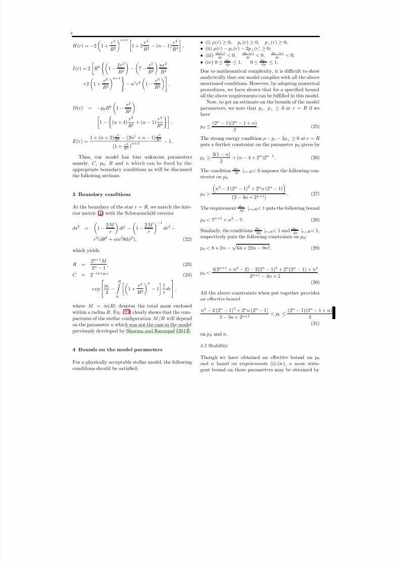
It is to be noted that for a real valued upper bound on p0 we must have n ≤ 4√

3. In Fig. 1, we have shown the

possible range of p0 and n (shaded region) for whicha physically acceptable stable stellar configuration is

possible.

Fig. 1 Bounds on the model parameters p0 and n basedon physical requirements and stability.

5 Physical analysis

Having derived a physically plausible model, let us nowanalyze the implications of the modified Finch and Skea

(1989) ansatz. Note that in our description, two of thefour unknown parameters can be determined from theboundary conditions (23) and (25) provided the mass isknown. Since the condition pr(R) = 0 is automaticallysatisfied, it provides no additional information aboutthe unknowns. Therefore, n and p

0 remain free param-

eters in our construction. For a chosen value of n, theparameter p0 can be appropriately fixed from withinthe bound provided in (35). Thus, all the physicallyinteresting quantities of the model can be evaluated if the mass M is supplied.

To examine the nature of physical quantities, wehave considered the pulsar 4U 1820 − 30 whose esti-mated mass and radius are given by M = 1.58 M ⊙ andR = 9.1 km, respectively Guver et al (2010a). Assum-ing M = 1.58 M ⊙, we note that if we set the dimension-less parameter n = 0.6154 and p0 = 0.1211 Mev fm−3,we get exactly the same radius as estimated by

Guver et al (2010a). Moreover, the compactness of the star can be made as high as ∼ 0.4543 for an up-per limit of n ∼ 1.38. Similarly, we have consideredsome other well studied pulsars like PSR J1903+327(Freire et al 2011), 4U 1608-52(Rawls et al 2011), VelaX-1(Rawls et al 2011), PSR J1614-2230(Demorest et al

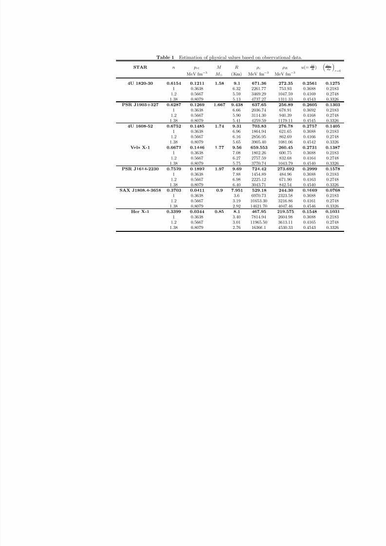
2010), SAX J1808.4-3658(Elebert 2009) and Her X-1(Abubekerov et al 2008) and shown that the estimatedmasses and radii of these stars can also be obtained bymaking necessary adjustments in the values of n. InTable 1, we have given the appropriate values of theadjustable compactness parameter n for which one can

obtain the predicted masses and radii of the stars con-sidered here. Respective central density (ρ0), surfacedensity (ρR), central pressure ( pr0 ) and compactness(u = M

R ) have also been shown in the table. The dif-ference in the values of these parameters for differentchoices of n has also been shown.

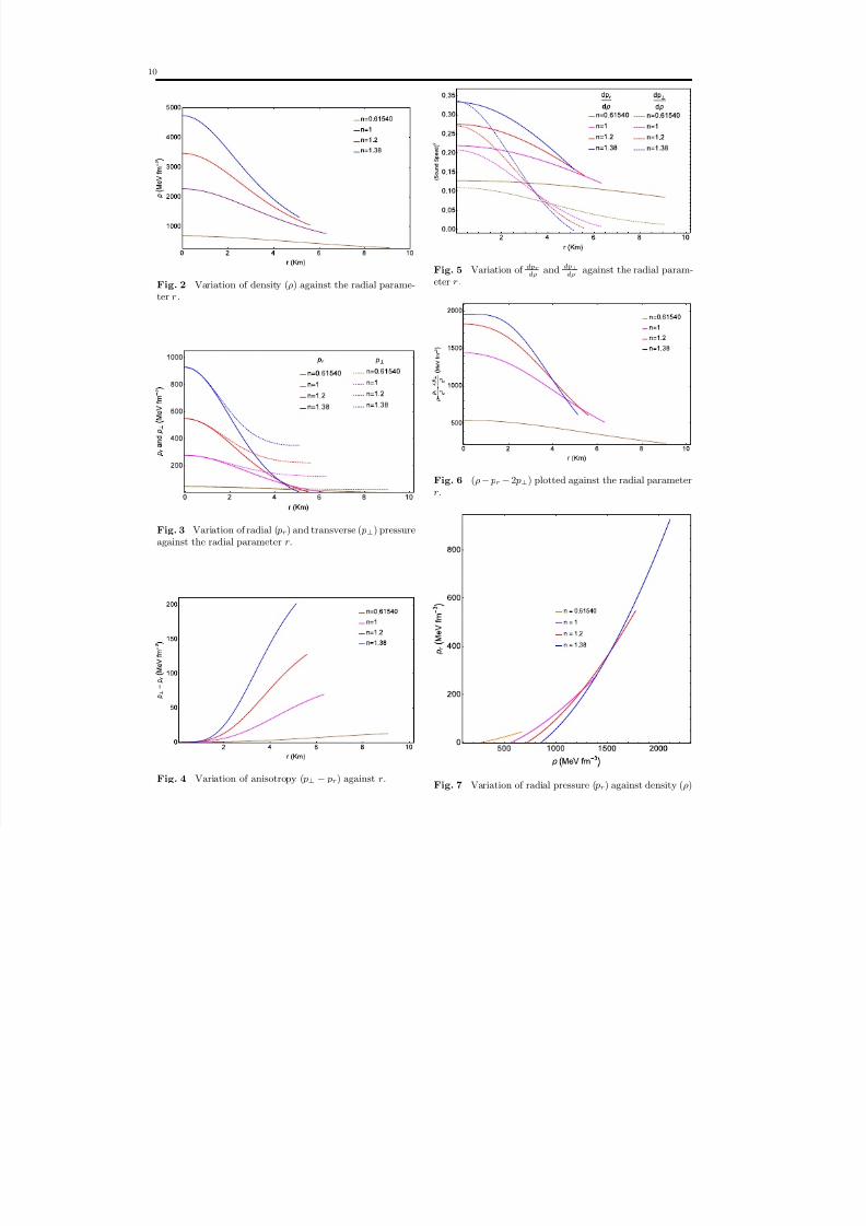
For a particular mass M = 1.58 M ⊙, we have alsoshown that all the physical quantities are well behavedat all interior points of the star within the specifiedbounds on n and p0. In Fig. 2, we have shown thevariation of density which shows that the density de-creases from its maximum value at the centre towards

the boundary. Moreover, the central density increasesif the value of n increases. In Fig. 3, radial variationof the two pressures has been shown. As expected, theradial pressure pr vanishes at the boundary; howeverthe tangential pressure p⊥ remains finite at the bound-ary. As in the case of density, both pressures increaseas n increases. In Fig. 4, radial variation of anisotropyhas been shown which shows that anisotropy is zero atthe centre and is maximum at the surface. In Fig. 5,radial variations of sound speed in the radial and trans-verse directions have been shown which confirms that



6

the causality condition is not violated throughout theconfiguration. In Fig. 6, we have plotted (ρ− pr−2 p⊥)which was shown to remain positive thereby implyingthat the strong energy condition is not violated in thismodel. Though we have not assumed any explicit EOSin our model, Fig. 7 shows how the radial pressurevaries against the density for different values of n.



Table 1 Estimation of physical values based on observational data.

STAR n pr0 M R ρc ρR u(= M R

)

MeV fm−3

M ⊙ (Km) MeV fm−3

MeV fm−3

4U 1820-30 0.6154 0.1211 1.58 9.1 671.36 272.35 0.2561

1 0.3638 6.32 2261.77 753.93 0.3688 1.2 0.5667 5.59 3469.29 1047.59 0.4169

1.38 0.8079 5.13 4737.27 1311.33 0.4543

PSR J1903+327 0.6287 0.1269 1.667 9.438 637.65 256.89 0.2605

1 0.3638 6.66 2036.74 678.91 0.3692 1.2 0.5667 5.90 3114.30 940.39 0.4168

1.38 0.8079 5.41 4259.59 1179.11 0.4545

4U 1608-52 0.6752 0.1485 1.74 9.31 703.83 276.78 0.2757

1 0.3638 6.96 1864.94 621.65 0.3688 1.2 0.5667 6.16 2856.95 862.69 0.4166

1.38 0.8079 5.65 3905.40 1081.06 0.4542

Vela X-1 0.6672 0.1446 1.77 9.56 659.553 260.45 0.2731 1 0.3638 7.08 1802.26 600.75 0.3688

1.2 0.5667 6.27 2757.59 832.68 0.4164 1.38 0.8079 5.75 3770.74 1043.79 0.4540

PSR J1614-2230 0.7529 0.1892 1.97 9.69 724.42 273.692 0.2999

1 0.3638 7.88 1454.89 484.96 0.3688 1.2 0.5667 6.98 2225.12 671.90 0.4163

1.38 0.8079 6.40 3043.71 842.54 0.4540

SAX J1808.4-3658 0.3703 0.0411 0.9 7.951 529.18 244.30 0.1669

1 0.3638 3.6 6970.73 2323.58 0.3688 1.2 0.5667 3.19 10653.30 3216.86 0.4161

1.38 0.8079 2.92 14621.70 4047.46 0.4546 Her X-1 0.3399 0.0344 0.85 8.1 467.95 219.575 0.1548

1 0.3638 3.40 7814.94 2604.98 0.3688

1.2 0.5667 3.01 11965.50 3613.11 0.4165 1.38 0.8079 2.76 16366.1 4530.33 0.4543



8

6 Discussion

In this paper, we have solved the Einstein’s field equa-tions describing a spherically symmetric anisotropicmatter composition by assuming the form of one of themetric potentials of the associated space-time and alsoby choosing a particular radial pressure profile. The as-sumed form of the metric potential is a generalizationof the Finch and Skea (1989) anzatz, which has so farbeen utilized successfully by many authors to generatesolutions to the Einstein’s field equations in differentastrophysical contexts. We note that a modificationof the Finch and Skea (1989) ansatz for the metric po-tential grr allows us to fit the theoretically obtainedcompactness to the observed compactness of a givenstar. We have shown that in the presence of such anadjustable parameter, it is possible to accommodate alarge class of observed pulsars in our model. Another

interesting feature of our approach is that though no apriori knowledge of the EOS is required in our set up, wehave been able to show that the predicted masses andradii of the pulsars based on the exotic strange matterEOS formulated by Dey et al (1998) and examined byGangopadhyay et al (2013) can also be fitted into ourmodel.

Acknowledgements

DMP is obliged for the support from the Inter-

University Centre for Astronomy and Astrophysics (IU-CAA), Pune, India, where a part of this work was car-ried out. RS acknowledges support from the IUCAA,under its Visiting Research Associateship Programme.DMP and VOT thank B S Ratanpal for useful sugges-tions.



9

References

Finch M. R. and Skea J. E. F., Class. Quantum Grav. 6

(1989) 467.Duorah H. L. and Ray R., Class. Quantum Gravity 4 (1987)

1691.

Delgaty M. S. R. and Lake K., Comput. Phys. Commun.115 (1998) 395;doi: http://dx.doi.org/10.1016/s0010-4655(98)00130-1.

Hansraj S. and Maharaj S. D., Int. J. Mod. Phys. D. 8

(2006) 1311.Tikekar R. and Jotania K., Gravitation and Cosmology 15

(2009) 129.Banerjee A., Rahaman F., Jotania K., Sharma R. and Karar

I., Gen. Revativ. Grav. 45 (2013) 717.Ruderman R., Astro. Astrophys. 10 (1972) 427.Canuto V., Annu. Rev. Astron. Astrophys. 12 (1974) 167.Bowers R. and Liang E., Astrophys. J. 188 (1974) 657.Maharaj S. D. and Marteens R., Gen. Relativ. Grav. 21

(1989) 899.

Gokhroo M. K. and Mehra A. L., Gen. Rel. Grav 26 (1994)75.

Patel L. K. and Mehta N. P., J. Indian Math. Soc. 61 (1995)95.

Tikekar R. and Thomas V. O., Pramana- j. of phys. 50

(1998) 95.Tikekar R. and Thomas V. O., Pramana-j. of phys. 52

(1999) 237.Tikekar R. and Thomas V. O., Pramana- j. of phys. 64

(2005) 5.Thomas V. O., Ratanpal B. S. and Vinodkumar P. C., Int.

J. Mod. Phys. D 14 (2005) 85.Thomas V. O. and Ratanpal B. S., Int. J. Mod. Phys. D 16

(2007) 9.

Dev K. and Gleiser M., Gen. Relativ. Grav. 34 (2002) 1793.Dev K. and Gleiser M., Gen. Rel. Grav. 35 (2003) 1435.Dev K. and Gleiser M., Int. J. Mod. Phys. D 13 (2004)

1389.Sharma R. and Maharaj S. D., Mon. Not. R. Astron. Soc.

375 (2007) 1265.Thirukkanesh S. and Maharaj S. D., Class. Quantum Grav.

25 (2008) 235001.Komathiraj K. and Maharaj S. D., Intenational Journal of

Modern Physics D 16 (2007) 1803.Sunzu J. M., Maharaj S. D., Ray S., Astrophys. Space Sci.

352 (2014) 719.Feroze T. and Siddiqui A. A., Gen. Relativ. Grav. 43 (2011)

1025.

Maharaj S. D. and Takisa P. M., Gen. Relativ. Grav. 44(2012) 1419.Varela V., Rahaman F., Ray S., Chakraborty K. and Kalam

M., Phys. Rev. D 82 (2010) 044052.Thirukkanesh S., Ragel F. S., Pramana J. Phys. 78 (2012)

687.Thirukkanesh S., Ragel F. S., Pramana J. Phys. 83 (2014)

83.Malaver M., Frontiers of Mathematics and its Applications

1 (2014) 9.Malaver M., American Journal of Astronomy and Astro-

physics 1 (2013) 41.Malaver M., World Applied Programming 3 (2013) 309.

Maharaj S. D. and Takisa P. M., Gen. Relativ. Grav. 45

(2013b) 1951.Nilsson, U.S., Uggla, C., Ann. Phys. 286 (2001) 292.Kinasiewicz, B., Mach, P., Acta Physica Polonica B 38

(2007).Heinzle, J.M., Rohr, N., Uggla, C., Class. Quantum Gravity

20 (2003) 4567.Paul B. C., Chattopadhyay P. K., Karmakar S. and Tikekar

R., Mod. Phys. Lett. A 26 (2011) 575.Sharma R. and Ratanpal B. S., Int. J. Mod. Phys. D 13

(2013) 1350074.Herrera L., Phys. Lett. A 165 (1992) 206.Guver T., Ozel F., Cabrera-Lavers A., Wroblewski P., ApJ.

712 (2010a) 964.Freire P. C. C. et al , Mon. Not. R. Astron. Soc. 412 (2011)

2763.Rawls M. L., Orosz J. A., McClintock J. E., Torres M. A.

P., Baliyn C. D., Buxton M. M., ApJ. 730 (2011) 25.Demorest P. B., Pennucci T., Ranson S. M., Rpberts M. S.

E., Hessels J. W. T., Nat. 467 (2010) 1081.

Elebert P. et al , Mon. Not. R. Astron. Soc. 395 (2009) 884.Abubekerov M. K., Antokhina E. A., Cherepashchuk A. M.,

Shimanskii V. V., Astron. Rep. 52 (2008) 379.Dey M., Bombaci I., Dey J., Ray S and Samanta B. C.,

Phys. Lett. B 438 (1998) 123.Gangopadhyay T., Ray S., Li X-D., Dey J. and Dey M.,

Mon. Not. R. Astron. Soc. 431 (2013) 3216.

This manuscript was prepared with the AAS LATEX macros v5.2.

http://dx.doi.org/10.1016/s0010-4655(98)00130-1

http://dx.doi.org/10.1016/s0010-4655(98)00130-1



10

Fig. 2 Variation of density (ρ) against the radial parame-ter r .

Fig. 3 Variation of radial ( pr) and transverse ( p⊥) pressureagainst the radial parameter r.

Fig. 4 Variation of anisotropy ( p⊥ − pr) against r.

Fig. 5 Variation of dprdρ

and dp⊥dρ

against the radial param-eter r .

Fig. 6 (ρ− pr−2 p⊥) plotted against the radial parameterr

.

Fig. 7 Variation of radial pressure ( pr) against density (ρ)

ArXiv Dishant Pandya

Documents

Transcript of ArXiv Dishant Pandya