Artiﬁcial-Noise-Aided Secure MIMO Wireless Communications ... · This paper considers a MIMO...

1

Artificial-Noise-Aided Secure MIMO Wireless

Communications via Intelligent Reflecting

Surface

Sheng Hong, Cunhua Pan, Hong Ren, Kezhi Wang, and Arumugam Nallanathan,

Fellow, IEEE

Abstract

This paper considers a MIMO secure wireless communication system aided by the physical layer

security technique of sending artificial noise (AN). To further enhance the system security performance, the

advanced intelligent reflecting surface (IRS) is invoked in the AN-aided communication system, where the

base station (BS), legitimate information receiver (IR) and eavesdropper (Eve) are equipped with multiple

antennas. With the aim for maximizing the secrecy rate (SR), the transmit precoding (TPC) matrix at the

BS, covariance matrix of AN and phase shifts at the IRS are jointly optimized subject to constrains of

transmit power limit and unit modulus of IRS phase shifts. Then, the secrecy rate maximization (SRM)

problem is formulated, which is a non-convex problem with multiple coupled variables. To tackle it, we

propose to utilize the block coordinate descent (BCD) algorithm to alternately update the TPC matrix,

AN covariance matrix, and phase shifts while keeping SR non-decreasing. Specifically, the optimal TPC

matrix and AN covariance matrix are derived by Lagrangian multiplier method, and the optimal phase

shifts are obtained by Majorization-Minimization (MM) algorithm. Since all variables can be calculated

in closed form, the proposed algorithm is very efficient. We also extend the SRM problem to the more

general multiple-IRs scenario and propose a BCD algorithm to solve it. Finally, simulation results validate

the effectiveness of system security enhancement via an IRS.

Index Terms

This work was supported by the National Natural Science Foundation of China (61661032), the Young Natural Science Foundation

of Jiangxi Province (20181BAB202002), the China Postdoctoral Science Foundation (2017M622102), the Foundation from China

Scholarship Council (201906825071).

S. Hong is with Information Engineering School of Nanchang University, Nanchang 330031, China. (email:

[email protected]). C. Pan, H. Ren, and A. Nallanathan are with the School of Electronic Engineering and Computer Science

at Queen Mary University of London, London E1 4NS, U.K. (e-mail:{c.pan, h.ren, a.nallanathan}@qmul.ac.uk). K. Wang is with

Department of Computer and Information Sciences, Northumbria University, UK. (email: [email protected]).

arX

iv:2

002.

0706

3v3

[ee

ss.S

P] 1

7 Ju

n 20

20

2

Intelligent Reflecting Surface (IRS), Reconfigurable Intelligent Surfaces, Secure Communication, Phys-

ical Layer Security, Artificial Noise (AN), MIMO.

I. INTRODUCTION

The next-generation (i.e, 6G) communication is expected to be a sustainable green, cost-effective

and secure communication system [1]. In particular, secure communication is crucially important

in 6G communication networks since communication environment becomes increasingly compli-

cated and the security of private information is imperative [2]. The information security using

crytographic encryption (in the network layer) is a conventional secure communication technique,

which suffers from the vulnerabilities, such as secret key distribution, protection and management

[3]. Unlike this network layer security approach, the physical layer security can guarantee good

security performance bypassing the relevant manipulations on the secret key, thus is more attractive

for the academia and industry [4]. There are various physical-layer secrecy scenarios. The first one

is the classical physical-layer secrecy setting where there is one legitimate information receiver

(IR) and one eavesdropper (Eve) operating over a single-input-single-output (SISO) channel (i.e.,

the so-called three-terminal SISO Gaussian wiretap channel) [5], [6]. The second one considers the

physical-layer secrecy with an IR and Eve operating over a multiple-input-single-output (MISO)

channel, which is called as three-terminal MISO Gaussian wiretap channel. The third one is a

renewed and timely scenario with one IR and one Eve operating over a multiple-input-multiple-

output (MIMO) channel, which is named as three-terminal MIMO Gaussian wiretap channel [7],

[8] and is the focus of this paper. For MIMO systems, a novel idea in physical-layer security is to

transmit artificial noise (AN) from the base station (BS) to contaminate the Eve’s received signal

[9]–[11]. For these AN-aided methods, a portion of transmit power is assigned to the artificially

generated noise to interfere the Eve, which should be carefully designed. For AN-aided secrecy

systems, while most of the existing AN-aided design papers focused on the MISO wiretap channel

and null-space AN [7], [12], designing the transmit precoding (TPC) matrix together with AN

covariance matrix for the MIMO wiretap channel is more challenging [13].

In general, the secrecy rate (SR) achieved by the mutual information difference between the

legitimate IR and the Eve is limited by the channel difference between the BS-IR link and the BS-

Eve link. The AN-aided method can further improve the SR, but it consumes the transmit power

destined for the legitimate IR. When the transmit power is confined, the performance bottleneck

always exists for the AN-aided secure communication. To conquer the dilemma, the recently

3

proposed intelligent reflecting surface (IRS) technique can be exploited. Since higher SR can be

achieved by enhancing the channel quality in the BS-IR link and degrading the channel condition in

the BS-Eve link, the IRS can serve as a powerful complement to AN-aided secure communication

due to its capability of reconfiguring the wireless propagation environment.

The IRS technique has been regarded as a revolutionary technique to control and reconfigure

the wireless environment [14], [15], [16]. An IRS comprises an array of reflecting elements,

which can reflect the incident electromagnetic (EM) wave passively, and the complex reflection

coefficient contains the phase shift and amplitude. In practical applications, the phase shifts of

the reflection coefficients are discrete due to the manufacturing cost [17]. However, many works

on IRS aided wireless communications are based on the assumption of continuous phase shifts

[18], [19]. To investigate the potential effect of IRS on the secure communication, we also

assume continuous phase shifts to simplify the problem. We evaluate its impact on the system

performance in the simulation section. Theoretically, the reflection amplitude of each IRS element

can be adjusted for different purpose [20]. However, considering the hardware cost, the reflection

amplitude is usually assumed to be 1 for simplicity. Hence, by smartly tuning the phase shifts with

a preprogrammed controller, the direct signals from the BS and the reflected signals from the IRS

can be combined constructively or destructively according to different requirements. In comparison

to the existing related techniques which the IRS resembles, such as active intelligent surface [21],

traditional reflecting surfaces [22], backscatter communication [23] and amplify-and-forward (AF)

relay [24], the IRSs have the advantages of flexible reconfiguration on the phase shifts in real

time, minor additional power consumption, easy installation with many reflecting elements, etc.

Furthermore, due to the light weight and compact size, the IRS can be integrated into the traditional

communication systems with minor modifications [25]. Because of these appealing virtues, IRS has

introduced into various wireless communication systems, including the single-user case [26], [27],

the downlink multiuser case [18], [28]–[31], mobile edge computing [32], wireless information

and power transfer design [33], and the physical layer security design [34]–[37].

IRS is promising to strengthen the system security of wireless communication. In [34], [36],

[38], the authors investigated the problem of maximizing the achievable SR in a secure MISO

communication system aided by IRS, where both the legitimate user and eavesdropper are equipped

with a single antenna. The TPC matrix at the BS and the phase shifts at the IRS were optimized

by an alternate optimization (AO) strategy. To handle the nonconvex unit modulus constraint, the

4

semidefinite relaxation (SDR) [39], majorization-minimization (MM) [18], [40], complex circle

manifold (CCM) [41] techniques were proposed to optimize phase shifts. An IRS-assisted MISO

secure communication with a single IR and single Eve was also considered in [35], but it was

limited to a special scenario, where the Eve has a stronger channel than the IR, and the two channels

from BS to Eve and IR are highly correlated. Under this assumption, the transmit beamforming

and the IRS reflection beamforming are jointly optimized to improve the SR. Similarly, a secure

IRS-assisted downlink MISO broadcast system was considered in [37], and it assumes that multiple

legitimate IRs and multiple Eves are in the same directions to the BS, which implies that the IR

channels are highly correlated with the Eve channels. [42] considered the transmission design for

an IRS-aided secure MISO communication with a single IR and single Eve, in which the system

energy consumption is minimized under two assumptions that the channels of access point (AP)-

IRS links are rank-one and full-rank. An IRS-assisted MISO network with cooperative jamming

was investigated in [2]. The physical layer security in a simultaneous wireless information and

power transfer (SWIPT) system was considered with the aid of IRS [43]. However, there are a

paucity of papers considering the IRS-assisted secure communication with AN. A secure MISO

communication system aided by the transmit jamming and AN was considered in [44], where a

large number of Eves exist, and the AN beamforming vector and jamming vector were optimized

to reap the additional degrees of freedom (DoF) brought by the IRS. [45] investigated the resource

allocation problem in an IRS-assisted MISO communication by jointly optimizing the beamforming

vectors, the phase shifts of the IRS, and AN covariance matrix for secrecy rate maximization

(SRM), but the direct BS-IRs links and direct BS-Eves link are assumed to be blocked.

Although a few papers have studied security enhancement for an AN-aided system through the

IRS, the existing papers related to this topic either only studied the MISO scenario or assumed

special settings to the channels. The investigation on the MIMO scenario with general channel

settings is absent in the existing literature. Hence, we investigate this problem in this paper by

employing an IRS in an AN-aided MIMO communication system for the physical layer security

enhancement. Specifically, by carefully designing the phase shifts of the IRS, the reflected signals

are combined with the direct signals constructively for enhancing the data rate at the IR and

destructively for decreasing the rate at the Eve. As a result, the TPC matrix and AN covariance

matrix at the BS can be designed flexibly with a higher DoF than the case without IRS. In this

work, the TPC matrix, AN covariance matrix and the phase shift matrix are jointly optimized.

5

Since these optimization variables are highly coupled, an efficient algorithm based on the block

coordinate descent (BCD) and MM techniques for solving the problem is proposed.

We summarize our main contributions as follows:

1) This is the first research on exploiting an IRS to enhance security in AN-aided MIMO

communication systems. Specifically, an SRM problem is formulated by jointly optimizing

the TPC matrix and AN covariance matrix at the BS, together with the phase shifts of

the IRS subject to maximum transmit power limit and the unit modulus constraint of the

phase shifters. The objective function (OF) of this problem is the difference of two Shannon

capacity expressions, thus is not jointly concave over the three highly-coupled variables. To

handle it, the popular minimum mean-square error (MMSE) algorithm is used to reformulate

the SRM problem.

2) The BCD algorithm is exploited to optimize the variables alternately. Firstly, given the

phase shifts of IRS, the optimal TPC matrix and AN covariance matrix are obtained in

closed form by utilizing the Lagrangian multiplier method. Then, given the TPC matrix

and AN covariance matrix, the optimization problem for IRS phase shifts is transformed

by sophisticated matrix manipulations into a quadratically constrained quadratic program

(QCQP) problem subject to unit modulus constraints. To solve it, the MM algorithm is

utilized, where the phase shifts are derived in closed form iteratively. Based on the BCD-

MM algorithm, the original formulated SRM problem can be solved efficiently.

3) The SRM problem is also extended to the more general scenario of multiple legitimate

IRs. A new BCD algorithm is proposed to solve it, where the optimal TPC matrix and AN

covariance matrix are obtained by solving a QCQP problem, and the unit modulus constraint

is handled by the penalty convex-concave procedure (CCP) method.

4) The simulation results confirm that on the one hand, the IRS can greatly enhance the security

of an AN-aided MIMO communication system; on the other hand, the phase shifts of

IRS should be properly optimized. Simulation results also show that larger IRS element

number and more transmit power is beneficial to the security. Moreover, properly-selected

IRS location and good channel states of the IRS-related links are important to realize the

full potential of IRS.

This paper is organized as follows. Section II provides the signal model of an AN-aided MIMO

communication system assisted by an IRS, and the SRM problem formulation. The SRM problem

6

is reformulated in Section III, where the BCD-MM algorithm is proposed to optimize the TPC

matrix, AN covariance matrix and phase shifts of IRS. Section IV extends the SRM problem to a

more general scenario of multiple IRs. In Section V, numerical simulations are given to validate

the algorithm efficiency and security enhancement. Section VI concludes this paper.

Notations: Throughout this paper, boldface lower case, boldface upper case and regular letters

are used to denote vectors, matrices, and scalars respectively. X�Y is the Hadamard product of

X and Y. Tr (X) and |X| denote the trace and determinant of X respectively. CM×N denotes the

space of M × N complex matrices. Re{·} and arg{·} denote the real part of a complex value

and the extraction of phase information respectively. diag{·} is the operator for diagonalization.

CN (µ,Z) represents a circularly symmetric complex gaussian (CSCG) random vector with mean

µ and covariance matrix Z. (·)T, (·)H and (·)∗ denote the transpose, Hermitian and conjugate

operators respectively. (·)? stands for the optimal value, and (·)† means the pseudo-inverse. [·]+ is

the projection onto the non-negative number, i.e, if y = [x]+, then y = max{0, x}.

II. SIGNAL MODEL AND PROBLEM FORMULATION

A. Signal Model

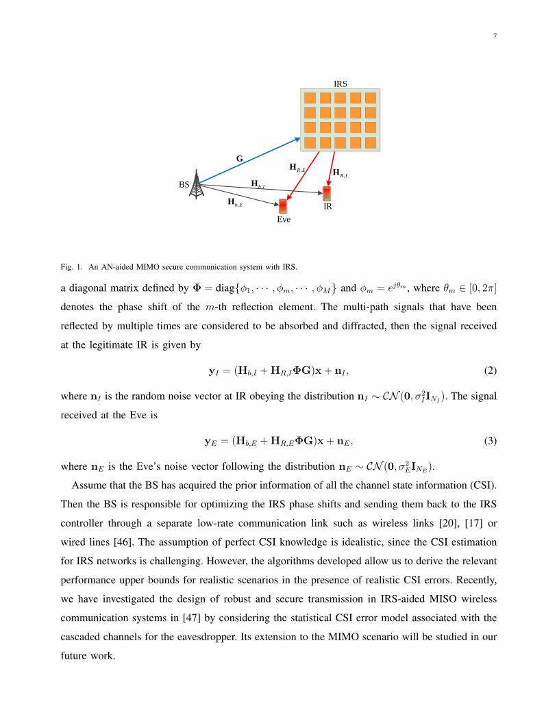
We consider an IRS-aided communication network shown in Fig. 1 that consists of a BS, a

legitimate IR and an Eve, all of which are equipped with multiple antennas. The number of

transmit antennas at the BS is NT ≥ 1, and the numbers of receive antennas at the legitimate IR

and Eve are NI ≥ 1 and NE ≥ 1 respectively. To ensure secure transmission from the BS to the

IR, the AN is sent from the BS to interfere the eavesdropper to achieve strong secrecy.

With above assumptions, the BS employed the TPC matrix to transmit data streams with AN.

The transmitted signal can be modeled as

x = Vs + n, (1)

where V ∈ CNT×d is the TPC matrix; the number of data streams is d ≤ min(NT , NI); the

transmitted data towards the IR is s ∼ CN (0, Id); and n ∈ CN (0,Z) represents the AN random

vector with zero mean and covariance matrix Z.

Assuming that the wireless signals are propagated in a non-dispersive and narrow-band way,

we model the equivalent channels of the BS-IRS link, the BS-IR link, the BS-Eve link, the IRS-

IR link, the IRS-Eve link by the matrices G ∈ CM×NT , Hb,I ∈ CNI×NT , Hb,E ∈ CNE×NT ,

HR,I ∈ CNI×M ,HR,E ∈ CNE×M , respectively. The phase shift coefficients of IRS are collected in

7

IRS

BS

IR

Eve

G

,b IH

,R EH,R IH

,b EH

Fig. 1. An AN-aided MIMO secure communication system with IRS.

a diagonal matrix defined by Φ = diag{φ1, · · · , φm, · · · , φM} and φm = ejθm , where θm ∈ [0, 2π]

denotes the phase shift of the m-th reflection element. The multi-path signals that have been

reflected by multiple times are considered to be absorbed and diffracted, then the signal received

at the legitimate IR is given by

yI = (Hb,I + HR,IΦG)x + nI , (2)

where nI is the random noise vector at IR obeying the distribution nI ∼ CN (0, σ2IINI

). The signal

received at the Eve is

yE = (Hb,E + HR,EΦG)x + nE, (3)

where nE is the Eve’s noise vector following the distribution nE ∼ CN (0, σ2EINE

).

Assume that the BS has acquired the prior information of all the channel state information (CSI).

Then the BS is responsible for optimizing the IRS phase shifts and sending them back to the IRS

controller through a separate low-rate communication link such as wireless links [20], [17] or

wired lines [46]. The assumption of perfect CSI knowledge is idealistic, since the CSI estimation

for IRS networks is challenging. However, the algorithms developed allow us to derive the relevant

performance upper bounds for realistic scenarios in the presence of realistic CSI errors. Recently,

we have investigated the design of robust and secure transmission in IRS-aided MISO wireless

communication systems in [47] by considering the statistical CSI error model associated with the

cascaded channels for the eavesdropper. Its extension to the MIMO scenario will be studied in our

future work.

8

Upon substituting x into (2), yI can be rewirtten as

yI = HI(Vs + n) + nI=HIVs + HIn + nI , (4)

where HI4= Hb,I + HR,IΦG is defined as the equivalent channel spanning from the BS to the

legitimate IR. Then, the data rate (bit/s/Hz) achieved by the legitimate IR is given by

RI(V,Φ,Z) = log∣∣∣I + HIVVHHH

I J−1I

∣∣∣ , (5)

where JI is the interference-plus-noise covariance matrix given by JI4= HIZHH

I + σ2IINI

.

Upon substituting x into (3), yE can be rewritten as

yE = HE(Vs + n) + nE = HEVs + HEn + nE, (6)

where HE4= Hb,E + HR,EΦG is defined as the equivalent channel spanning from the BS to the

Eve. Then, the data rate (bit/s/Hz) achieved by the Eve is given by

RE(V,Φ,Z) = log∣∣∣I + HEVVHHH

EJ−1E

∣∣∣ , (7)

where JE is the interference-plus-noise covariance matrix given by JE4= HEZHH

E + σ2EINE

. The

achievable secrecy rate is given by

CAN(V,Φ,Z)=[RI(V,Φ,Z)−RE(V,Φ,Z)]+

= log∣∣∣I + HIVVHHH

I J−1I

∣∣∣− log∣∣∣I + HEVVHHH

EJ−1E

∣∣∣= log

∣∣∣I + HIVVHHHI (HIZHH

I + σ2IINI

)−1∣∣∣

− log∣∣∣I + HEVVHHH

E (HEZHHE + σ2

EINE)−1∣∣∣ . (8)

B. Problem Formulation

With the aim for maximizing SR, the TPC matrix V at the BS, the AN covariance matrix

Z at the BS, and the phase shift matrix Φ at the IRS should be optimized jointly subject to the

constraints of the maximum transmit power and unit modulus of phase shifts. Hence, we formulate

the SRM problem as

maxV,Φ,Z

CAN(V,Φ,Z) (9a)

s.t. Tr(VVH+Z) ≤ PT , (9b)

Z � 0, (9c)

|φm| = 1,m = 1, · · · ,M, (9d)

9

where PT is the maximum transmit power limit. The optimal value of SR in (9) is always non-

negative, which can be proved by using contradiction. Assume that the optimal value of SR is

negative, then we can simply set the TPC matrix V to zero matrix, and the resulted SR will be

equal to zero, which is larger than a negative SR.

By variable substitution Z = VEVHE , where VE ∈ CNT×NT , Problem (9) is equivalent to

maxV,VE ,Φ

CAN(V,VE,Φ) (10a)

s.t. Tr(VVH+VEVHE ) ≤ PT , (10b)

|φm| = 1,m = 1, · · · ,M, (10c)

where the OF of (10a) is obtained by substituting Z = VEVEH into (8). In (10a), the expression

of OF is difficult to tackle, and the variables of V, VE and Φ are coupled with each other, which

make Problem (10) difficult to solve. In addition, the unit modulus constraint imposed on the phase

shifts in (10c) aggravates the difficulty. In the following, we provide a low-complexity algorithm

to solve this problem.

III. A LOW-COMPLEXITY ALGORITHM OF BCD-MM

Firstly, the OF of Problem (10) is reformulated into a more tractable expression equivalently.

Then, the BCD-MM method is proposed for optimizing the TPC matrix V, VE , and the phase

shift matrix Φ alternately.

A. Reformulation of the Original Problem

Firstly, the achievable SR CAN(V,VE,Φ) in (8) can be further simplified as

CAN(V,VE,Φ)= log∣∣∣INI

+ HIVVHHHI (HIZHH

I + σ2IINI

)−1∣∣∣+log

∣∣∣HEZHHE + σ2

EINE

∣∣∣− log

∣∣∣HEZHHE + σ2

EINE+ HEVVHHH

E

∣∣∣= log

∣∣∣INI+ HIVVHHH

I (HIVEVHE HH

I + σ2IINI

)−1∣∣∣︸︷︷︸

f1

+ log∣∣∣INE

+ HEVEVHE HH

E (σ2EINE

)−1∣∣∣︸︷︷︸

f2

−log∣∣∣INE

+ σ−2E HE(VVH + VEVH

E )HHE

∣∣∣︸︷︷︸f3

. (11)

10

The expression in f1 represents the data rate of the legitimate IR, which can be reformulated by

exploiting the relationship between the data rate and the mean-square error (MSE) for the optimal

decoding matrix. Specifically, the linear decoding matrix UI ∈ CNT×d is applied to estimate the

signal vector s for the legitimate IR, and the MSE matrix of the legitimate IR is given by

EI(UI ,V,VE)∆= Es,n,nI

[(s− s)(s− s)H

]=(UI

HHIV − Id)(UIHHIV − Id)

H + UIH(HIVEVE

HHHI +σ2

IINI)UI . (12)

By introducing an auxiliary matrix WI � 0, WI ∈ Cd×d and exploiting the fact 3) of Lemma 4.1

in [48], we have

f1= maxUI ,WI�0

h1(UI ,V,VE,WI)

∆= max

UI ,WI�0log |WI | − Tr(WIEI(UI ,V,VE)) + d. (13)

h1(UI ,V,VE,WI) is concave with respect to (w.r.t.) each matrix of the matrices UI ,V,VE ,WI

by fixing the other three matrices. According to the facts 1) and 2) of Lemma 4.1 in [48], the

optimal U?I , W?

I to achieve the maximum value of h1(UI ,V,VE,WI) is given by

U?I=arg max

UI

h1(UI ,V,VE,WI)=(HIVEVHE HH

I +σ2IINI

+HIVVHHHI )−1HIV, (14)

W?I=arg max

WI�0h1(UI ,V,VE,WI)= [E?

I(U?I ,V,VE)]−1, (15)

where E?I is obtained by plugging the expression of U?

I into EI(UI ,V,VE) as

E?I(U

?I ,V,VE)=(U?H

I HIV − Id)(U?HI HIV − Id)

H + U?HI (HIVEVH

E HHI +σ2

IINI)U?

I . (16)

Similarly, by introducing the auxiliary variables WE � 0, WE ∈ CNT×NT , UE ∈ CNE×NT , and

exploiting the fact 3) of Lemma 4.1 in [48], we have

f2= maxUE ,WE�0

h2(UE,VE,WE)

∆= max

UE ,WE�0log |WE| − Tr(WEEE(UE,VE)) +Nt, (17)

h2(UE,VE,WE) is concave w.r.t each matrix of the matrices UE ,VE ,WE when the other two

matrices are given. According to the facts 1) and 2) of Lemma 4.1 in [48], the optimal U?E , W?

E

to achieve the maximum value of h2(UE,VE,WE) is given by

U?E=arg max

UE

h2(UE,VE,WE)=(σ2EINE

+HEVEVHE HH

E )−1HEVE, (18)

11

W?E=arg max

WE�0h2(UE,VE,WE)= [E?

E(U?E,VE)]−1, (19)

where E?E is obtained by plugging the expression of U?

E into EE(UE,VE) as

E?E(U?

E,VE) = (UE?HHEVE − INT

)(U?HE HEVE − INT

)H + U?HE (σ2

EINE)U?

E. (20)

By using the Lemma 1 in [13], we have

f3= maxWX�0

h3(V,VE,WX)

= maxWX�0

log |WX | − Tr(WXEX(V,VE)) +NE, (21)

where WX � 0, WX ∈ CNE×NE are the introduced auxiliary variable, and

EX(V,VE)∆= INE


E )HHE . (22)

h3(V,VE,WX) is concave w.r.t each matrix of the matrices V,VE,WX when the other two

matrices are given. The optimal W?X to achieve the maximum value of h3(V,VE,WX) is

W?X=arg max

WX�0h3(V,VE,WX)= [EX(V,VE)]−1. (23)

By substituting (13), (17), (21) into (11), we have

CAN(V,VE) = arg maxUI ,WI ,UE ,WE ,WX

ClAN(UI ,WI ,UE,WE,WX ,V,VE), (24)

where

ClAN(UI ,WI ,UE,WE,WX ,V,VE)

∆=h1(UI ,V,VE,WI) + h2(UE,VE,WE)

+ h3(V,VE,WX). (25)

Obviously, ClAN(UI ,WI ,UE,WE,WX ,V,VE) is a concave function for each of the matrices

UI ,WI ,UE ,WE ,WX ,V,VE when the other six matrices are given. By substituting (24) into

Problem (10), we have the following equivalent problem:

maxUI ,WI�0,UE ,WE�0,WX�0,V,VE ,Φ

ClAN(UI ,WI ,UE,WE,WX ,V,VE,Φ) (26a)

s.t. Tr(VVH+VEVEH) ≤ PT , (26b)

|φm| = 1,m = 1, · · · ,M. (26c)

To solve Problem (26), we apply the BCD method, each iteration of which consists the following

two sub-iterations. Firstly, with given V,VE,Φ, update UI ,WI ,UE,WE,WX by using (14),

12

(15), (18), (19), (23) respectively. Secondly, with given UI ,WI ,UE,WE,WX , update V,VE,Φ

by solving the following subproblem:

minV,VE ,Φ

− Tr(WIVHHH

I UI)− Tr(WIUHI HIV) + Tr(VHHV V)

− Tr(WEVHE HH

EUE)− Tr(WEUHE HEVE) + Tr(VH

EHV EVE) (27a)


|φm| = 1,m = 1, · · · ,M, (27c)

where

HV = HHI UIWIU

HI HI + σ−2

E HHEWXHE, (28)

HV E = HHI UIWIU

HI HI + HH

EUEWEUHE HE + σ−2

E HHEWXHE. (29)

Problem (27) is obtained from Problem (26) by taking the UI ,WI ,UE,WE,WX as constant

values, and the specific derivations are given in Appendix A.

It is obvious that Problem (27) is much easier to tackle than Problem (10) due to the convex

quadratic OF in (27a). Now, we devote to solve Problem (27) equivalently instead of Problem (10),

and the matrices V, VE , and phase shift matrix Φ will be optimized.

B. Optimizing the Matrices V and VE

In this subsection, the TPC matrix V and matrix VE are optimized by fixing Φ. Specifically, the

unit modulus constraint on the phase shifts Φ is removed, and the updated optimization problem

reduced from Problem (27) is given by

minV,VE

− Tr(WIVHHH

I UI)− Tr(WIUHI HIV) + Tr(VHHV V)

− Tr(WEVHE HH

EUE)− Tr(WEUHE HEVE) + Tr(VH

EHV EVE) (30a)

s.t. Tr(VVH+VEVHE ) ≤ PT . (30b)

The above problem is a convex QCQP problem, and the standard optimization packages, such

as CVX [49] can be exploited to solve it. However, the calculation burden is heavy. To reduce

the complexity, the near-optimal closed form expressions of the TPC matrix and AN covariance

matrix are provided by applying the Lagrangian multiplier method.

Since Problem (30) is a convex problem, the Slater’s condition is satisfied, where the duality gap

between Problem (30) and its dual problem is zero. Thus, Problem (30) can be solved by addressing

13

its dual problem if the dual problem is easier. For this purpose, by introducing Lagrange multiplier

λ to combine the the constraint and OF of Problem (30), the Lagrangian function of Problem (30)

is obtained as

L (V,VE, λ)∆=−Tr

(WIV

HHHI UI

)−Tr

(WIU

HI HIV

)+Tr

(VHHV V

)−Tr

(WEVH

E HHEUE

)− Tr

(WEUH

E HEVE

)+ Tr

(VHEHV EVE

)+ λ[Tr

(VVH + VEVH

E

)− PT ]

= −Tr(WIV

HHHI UI

)− Tr

(WIU

HI HIV

)+ Tr

[VH (HV + λI) V

]− Tr

(WEVH

E HHEUE

)−Tr

(WEUH

E HEVE

)+Tr

[VHE (HV E+λI) VE

]−λPT .

(31)

Then the dual problem of Problem (30) is

maxλ

h (λ) (32a)

s.t. λ ≥ 0, (32b)

where h (λ) is the dual function given by

h (λ)∆= min

V,VE

L (V,VE, λ) . (33)

Note that Problem (33) is a convex quadratic optimization problem with no constraint, which can

be solved in closed form. The optimal solution V?,V?E for Problem (33) is

[V?,V?E] = arg min

V,VE

L (V,VE, λ) . (34)

By setting the first-order derivative of L (V,VE, λ) w.r.t. V to zero matrix, we can obtain the

optimal solution of V as follows:

∂L (V,VE, λ)

∂V= 0, (35a)

∂L (V,VE, λ)

∂VE

= 0. (35b)

The left hand side of Equation (35a) can be expanded as

∂L (V,VE, λ)

∂V=∂Tr

[VH (HV + λI) V

]∂V

−(WIU

HI HI

)H−(HHI UIWI

)= 2 (HV + λI) V − 2

(HHI UIWI

). (36)

The equation (35a) becomes

(HV + λI) V =(HHI UIWI

). (37)

14

Then the optimal solution V? for Problem (34) is

V? = (HV + λI)†(HHI UIWI

)∆= ΘV (λ)

(HHI UIWI

). (38)

Similarly, we solve Problem (34) by setting the first-order derivative of L (V,VE, λ) w.r.t. VE to

zero matrix, which becomes

2 (HV E + λI) VE − 2HHEUEWH

E = 0. (39)

Then the optimal solution V?E for Problem (34) is

V?E = (HV E + λI)† HH

EUEWHE

∆= ΘV E (λ) HH

EUEWHE . (40)

Once the optimal solution λ? for Problem (32) is found, the final optimal V?,V?E can be obtained.

The value of λ? should be chosen in order to guarantee the complementary slackness condition as

λ[Tr(V?V?H+V?EV?H

E )− PT ] = 0. (41)

We define

P (λ)∆= Tr(V?V?H+V?

EV?HE ) = Tr(V?V?H) + Tr(V?

EV?HE ), (42)

where

Tr(V?V?H

)= Tr

(ΘV (λ) (HH

I UIWHI )(HH

I UIWHI )HΘH

V (λ))

= Tr(ΘHV (λ) ΘV (λ) (HH

I UIWHI )(HH

I UIWHI )H

), (43)

Tr(V?HE V?

E

)= Tr

(ΘV E (λ) (HH

EUEWHE )(HH

EUEWHE )HΘH

V E (λ))

= Tr(ΘHV E (λ) ΘV E (λ) (HH

EUEWHE )(HH

EUEWHE )H

). (44)

Then P (λ) becomes

P (λ) = Tr(ΘnV (HH

I UIWHI )(HH

I UIWHI )H

)+ Tr

(ΘnV E(HH

EUEWHE )(HH

EUEWHE )H

), (45)

where

ΘnV = ΘH

V (λ) ΘV (λ) = (HV + λI)†H (HV + λI)† , (46)

15

ΘnV E = ΘH

V E (λ) ΘV E (λ) = (HV E + λI)†H (HV E + λI)† . (47)

To find the optimal λ? ≥ 0, we first check whether λ = 0 is the optimal solution or not. If

P (0) = Tr(V?H(0)V?(0)

)+ Tr

(V?HE (0)VE

?(0))≤ PT , (48)

then the optimal solutions are given by V? = V(0) and V?E = VE(0). Otherwise, the optimal

λ? > 0 is the solution of the equation P (λ) = 0.

It is ready to verify that HV and HV E is a positive semidefinite matrix. Let us define the

rank of HV and HV E as rV = rank(HV ) ≤ NT and rV E = rank(HV E) ≤ NT respectively. By

decomposing HV and HV E by using the singular value decomposition (SVD), we have

HV = [PV,1,PV,2] ΣV [PV,1,PV,2]H,HV E = [PV E,1,PV E,2] ΣV E[PV E,1,PV E,2]H, (49)

where PV,1 comprises the first rV singular vectors associated with the rV positive eigenvalues of

HV , and PV,2 includes the last NT − rV singular vectors associated with the NT − rV zero-valued

eigenvalues of HV , ΣV = diag{ΣV,1,0(NT−rV )×(NT−rV )

}with ΣV,1 representing the diagonal

submatrix collecting the first rV positive eigenvalues. Similarly, the first rV E singular vectors

corresponding to the rV E positive eigenvalues of HV E are contained in PV E,1, while the last

NT−rV E singular vectors corresponding to the NT−rV E zero-valued eigenvalues of HV E are held

in PV E,2. ΣV E = diag{ΣV E,1,0(NT−rV E)×(NT−rV E)

}is a diagonal matrix with ΣV E,1 representing

the diagonal submatrix gathering the first rV E positive eigenvalues. By defining PV∆= [PV,1,PV,2]

and PV E∆= [PV E,1,PV E,2], and substituting (49) into (46) and (47), P (λ) becomes

P (λ) = Tr(

[(PV ΣV PH

V + λPV PHV

)−1(PV ΣV PH

V + λPV PHV

)−1](HH

I UIWHI )(HH

I UIWHI )H

)+Tr

([(PV EΣV EPH

V E+λPV EPHV E

)−1(PV EΣV EPH

V E+λPV EPHV E

)−1](HH

EUEWHE)(HH

EUEWHE )H)

= Tr([(ΣV + λI)−2]ZV

)+ Tr

([(ΣV E + λI)−2]ZV E

)=

rV∑i=1

[ZV ]i,i([ΣV ]i,i+λ

)2

+

rV E∑i=1

[ZV E]i,i([ΣV E]i,i+λ

)2

+

NT∑i=rV +1

[[ZV ]i,i

(λ)2

]+

NT∑i=rV E+1

[[ZV E]i,i

(λ)2

], (50)

where ZV = PHV (HH

I UIWHI )(HH

I UIWHI )HPV and ZV E = PH

V E(HHEUEWH

E )(HHEUEWH

E )HPV E .

[ZV ]i,i, [ZV E]i,i, [ΣV ]i,i, and [ΣV E]i,i represent the ith diagonal element of matrices ZV , ZV E , ΣV ,

and ΣV E , respectively. The first line of (50) is obtained by substituting (49) into the expression of

P (λ) in (45). It can be verified from the last line of (50) that P (λ) is a monotonically decreasing

function.

16

Then, the optimal λ? can be obtained by solving the following equation,

rV∑i=1

[ZV ]i,i([ΣV ]i,i + λ

)2

+

rV E∑i=1

[ZV E]i,i([ΣV E]i,i + λ

)2

+

NT∑i=rV +1

[[ZV ]i,i

(λ)2

]+

NT∑i=rV E+1

[[ZV E]i,i

(λ)2

]= PT . (51)

To solve it, the bisection search method is utilized. Since P (∞) = 0, the solution to Equation (51)

must exist. The lower bound of λ? is a positive value approaching zero, while the upper bound of

λ? is given by

λ? <

√√√√√NT∑i=1

[ZV ]i,i +NT∑i=1

[ZV E]i,i

PT

∆= λub. (52)

which can be proved as

P (λub) =

rV∑i=1

[ZV ]i,i([ΣV ]i,i + λub

)2 +

rV E∑i=1

[ZV E]i,i([ΣV E]i,i + λub

)2 +

NT∑i=rV +1

[[ZV ]i,i

(λub)2

]+

NT∑i=rV E+1

[[ZV E]i,i

(λub)2

]

<

NT∑i=1

[ZV ]i,i

(λub)2 +

NT∑i=1

[ZV E]i,i

(λub)2 = PT . (53)

When the optimal λ? is found, the optimal matrices V? and V?E can be obtained by substituting

λ? into (38) and (40).

C. Optimizing the Phase Shifts Φ

In this subsection, the phase shift matrix Φ is optimized by fixing V and VE . The transmit

power constraint in Problem (27) is only related with V and VE , thus is removed. Then, the

optimization problem for Φ reduced from Problem (27) is formulated as

minΦ

g0(Φ)∆= −Tr(WIV

HHHI UI)− Tr(WIUI

HHIV) + Tr(VHHV V)

− Tr(WEVEHHH

EUE)− Tr(WEUEHHEVE) + Tr(VE

HHV EVE) (54a)

s.t. |φm| = 1,m = 1, · · · ,M. (54b)

By the aid of complex mathematical manipulations, which are given in details in Appendix B,

Problem (54) can be transformed into a form that can facilitate the MM algorithm. Based on the

derivations in Appendix B, the OF g0(Φ) can be equivalently transformed into

g0(Φ) = Tr(ΦHDH

)+ Tr (ΦD) + Tr

[ΦHBV EΦCV E

]+ Tr

(ΦHBV ΦCV

)+ Ct, (55)

where Ct, D, CV E , CV , BV E and BV are constants for Φ, and are given in Appendix B.

17

By exploiting the matrix properties in [50, Eq. (1.10.6)], the trace operators can be removed,

and the third and fourth terms in (55) become as

Tr(ΦHBV EΦCV E

)= φH

(BV E �CT

V E

)φ, (56a)

Tr(ΦHBV ΦCV

)= φH

(BV �CT

V

)φ, (56b)

where φ∆=[ejθ1 , · · · , ejθm , · · · , ejθM

]T is a vector holding the diagonal elements of Φ.

Similarly, the trace operators can be removed for the first and second terms in (55) as

Tr(ΦHDH

)= dH(φ∗),Tr (ΦD) = φTd, (57)

where d =[[D]1,1, · · · , [D]M,M

]T

is a vector gathering the diagonal elements of matrix D.

Hence, Problem (54) can be rewritten as

minφ

φHΞφ + φTd + dH(φ∗) (58a)

s.t. |φm| = 1,m = 1, · · · ,M, (58b)

where Ξ = BV E � CTV E + BV � CT

V . Ξ is a semidefinite matrix, because it is a sum of two

semidefinite matrices, both of which are Hadamard products of two semidefinite matrices. It is

observed that BV E , CTV E , BV and CT

V are semidefinite matrices. Then, the Hadamard products of

BV E �CTV E and BV �CT

V are semidefinite according to the Property (9) on Page 104 of [50].

Problem (58) can be further simplified as

minφ

f(φ)∆= φHΞφ + 2Re

{φH(d∗)

}(59a)

s.t. |φm| = 1,m = 1, · · · ,M. (59b)

The Problem (59) can be solved by the SDR technique [28] by transforming the unimodulus

constraint into a rank-one constraint, however, the rank-one solution cannot always be obtained

and the computation complexity is heavy for the SDR method. Thus, we propose to solve Problem

(59) efficiently by the MM algorithm as [25], where the closed-form solution can be obtained in

each iteration. Details are omitted for simplicity.

D. Overall Algorithm to Solve Problem (10)

To sum up, the detailed execution of the overall BCD-MM algorithm proposed for solving

Problem (10) is provided in Algorithm 1. The MM algorithm is exploited for solving the optimal

phase shifts Φ(n+1) of Problem (59) in Step 5. The iteration process in MM algorithm ensures

18

that the OF value of Problem (59) decreases monotonically. Moreover, the BCD algorithm also

guarantees that the OF value of Problem (27) monotonically decreases in each step and each

iteration of Algorithm 1. Since the OF value in (27a) has a lower bound with the power limit, the

convergence of Algorithm 1 is guaranteed.

Algorithm 1 BCD-MM Algorithm1: Parameter Setting. Set the maximum number of iterations nmax and the first iterative number

n = 1; Give the error tolerance ε.

2: Variables Initialization. Initialize the variables V(1), V(1)E and Φ(1) in the feasible region;

Compute the OF value of Problem (10) as OF(V(1),V(1)E ,Φ(1));

3: Auxiliary Variables Calculation. Given V(n),V(n)E , Φ(n), compute the optimal matrices

U(n)I ,W

(n)I ,U

(n)E ,W

(n)E ,W

(n)X according to (14), (15), (18), (19), (23) respectively;

4: Matrices Optimization. Given U(n)I ,W

(n)I ,U

(n)E ,W

(n)E ,W

(n)X , solve the optimal TPC matrix

V(n+1) and equivalent AN covariance matrix V(n+1)E of Problem (34) with the Lagrangian

multiplier method;

5: Phase Shifts Optimization. Given U(n)I ,W

(n)I ,U

(n)E ,W

(n)E ,W

(n)X and V(n+1),V

(n+1)E , solve the

optimal phase shifts Φ(n+1) of Problem (59) with the MM algorithm;

6: Termination Check. If∣∣∣OF(V(n+1),V

(n+1)E ,Φ(n+1))−OF(V(n),V

(n)E ,Φ

(n))∣∣∣/OF(V(n+1),V

(n+1)E ,Φ(n+1))<

ε or n ≥ nmax, terminate. Otherwise, update n← n+ 1 and jump to step 2.

Based on the algorithm description, the complexity analysis of the proposed BCD-MM algorithm

is performed. In Step 3, computing the decoding matrices U(n)I and U

(n)E costs the complexity of

O(N3I ) + O(N3

E), while calculating the auxiliary matrices W(n)I , W

(n)E , and W

(n)X consumes the

complexity of O(d3) + O(N3T ) + O(N3

E). The complexity of calculating the TPC matrix V(n+1)

and AN covariance matrix V(n+1)E in Step 4 can be analyzed according to the specific process of

Lagrangian multiplier method based on the fact that the complexity of computing product XY of

complex matrices X ∈ Cm×n and Y ∈ Cn×p is O (mnp). By assuming that NT > NI(or NE) > d,

the complexity of computing the matrices {HV ,HV E} in (28) and (29) is O(N3T ) +O(2N2

Td) +

O(2N2TNE); while the complexity of calculating V∗, V∗E in (38) and (40) is O(2N3

T ). The SVD

decomposition of {HV ,HV E} requires the computation complexity of O(2N3T ), while calculating

{ZV } and {ZV E} requires the complexity of O(N2TNI) + O(2N3

T ). The complexity of finding

the Lagrangian multipliers {λ} is negligible. Thus, the overall complexity for V(n+1), V(n+1)E is

19

about O(max{2N3T , 2N

2TNE}). In step 5, obtaining optimal Φ(n+1) by the MM algorithm need a

complexity of CMM = O(M3 + TMMM2), where TMM is the iteration number for convergence.

Based on the complexity required in Step 3, 4 and 5, the overall complexity CBCD−MM of the

BCD-MM algorithm can be evaluated by

CBCD−MM = O(max{2N3T , 2N

2TNE, CMM}). (60)

IV. EXTENSION TO THE MULTIPLE-IRS SCENARIO

A. Problem Formulation

Consider a multicast extension where there are L ≥ 2 legitimate IRs, and they all intend to

receive the same message. The signal model for the MIMO multi-IRs wiretap channel scenario is

yI,l = HI,l(Vs + n) + nI,l, l = 1, · · · , L, (61)

where HI,l4= Hb,I,l + HR,I,lΦG. The subscript l indicates the lth IR, and the other notations are

the same as (4) and (6). Under these settings, the achievable SR is given by [51]

Rs(V,VE,Φ) = minl=1,··· ,L

{RI,l(V,Φ,Z)−RE(V,Φ,Z)}, (62)

where RI,l(V,Φ,Z) = log∣∣∣I + HI,lVVHHH

I,lJ−1I,l

∣∣∣ and JI,l4= HI,lZHH

I,l + σ2I,lINI

.

Then the multicast counterpart of the AN-aided SRM problem (10) is formulated as

maxV,VE ,Φ

Rs(V,VE,Φ) (63a)


|φm| = 1,m = 1, · · · ,M. (63c)

The objective function of Problem (63) can be rewritten as

Rs(V,VE,Φ) = minl=1,··· ,L

{log∣∣∣INI

+ HI,lVVHHHI,l(HI,lVEVH

E HHI,l + σ2

I,lINI)−1∣∣∣︸︷︷︸

f1,l

}

+ log∣∣∣INE

+ HEVEVHE HH

E (σ2EINE

)−1∣∣∣︸︷︷︸

f2

−log∣∣∣INE


E )HHE

∣∣∣︸︷︷︸f3

, (64a)

= minl=1,··· ,L

{ maxUI,l,WI,l�0

h1,l(UI,l,V,VE,WI,l)}+ maxUE ,WE�0

h2(UE,VE,WE)

+ maxWX�0

h3(V,VE,WX). (64b)

20

The lower bound to the first term of (64b) can be found as

minl=1,··· ,L

{ maxUI,l,WI,l�0

h1,l(UI,l,V,VE,WI,l)} (65a)

≥ max{UI,l,WI,l�0}Ll=1

{ minl=1,··· ,L

h1,l(UI,l,V,VE,WI,l)}, (65b)

where (65b) holds due to the fact that minx

maxyf(x, y) ≥ max

yminxf(x, y) for any function f(x, y).

Here by exchanging the positions of max{UI,l,WI,l�0}Ll=1

and minl=1,··· ,L

in (65a), we can find a lower bound

to Rs(V,VE,Φ) as

fms(V,VE, {UI,l,WI,l}Ll=1,UE,WE,WX)

, maxV,VE ,{UI,l,WI,l�0}Ll=1,UE ,WE�0,WX�0

{ minl=1,··· ,L

h1,l(UI,l,V,VE,WI,l)

+ h2(UE,VE,WE) + h3(V,VE,WX)}. (66)

We simplify Problem (63) by maximizing a lower bound to its original objective as follows,

maxV,VE ,Φ,{UI,l,WI,l�0}Ll=1,UE ,WE�0,WX�0

fms(V,VE, {UI,l,WI,l}Ll=1,UE,WE,WX) (67a)


|φm| = 1,m = 1, · · · ,M. (67c)

To solve the multicast AN-aided SRM problem in (67), a BCD-QCQP-CCP algorithm is proposed.

B. BCD Iterations for Problem (67)

The equivalent SRM problem in (67) provides a desirable formulation for BCD algorithm. In

particular, one can show that problem (67) is convex w.r.t. either V,VE or Φ or {UI,l, WI,l}Ll=1,

UE , WE , WX . By fixing Φ, the iteration process for problem (67) is as follows. Let Vn, VnE ,

{UnI,l,W

nI,l}Ll=1,U

nE,W

nE,W

nX denote the BCD iterate at the nth iteration. The BCD iterates are

21

generated via

UnI,l = arg max

UI,l

h1,l(UI,l,Vn,Vn

E,WnI,l)

=(HI,lVnEVnH

E HHI,l+σ

2I,lINI

+HI,lVnVnHHH

I,l)−1HI,lV

n, (68a)

WnI,l = arg max

WI,l�0h1,l(U

nI,l,V

n,VnE,WI,l)= [EI,l(U

nI,l,V

n,VnE)]−1

=[(UnHI,l HI,lV

n − Id)(UnHI,l HI,lV

n − Id)H + UnH

I,l (HI,lVnEVnH

E HHI,l+σ

2I,lINI

)UnI,l]−1, (68b)

UnE=arg max

UE

h2(UE,VnE,W

nE)

=(σ2EINE

+HEVnEVnH

E HHE )−1HEVn

E, (68c)

WnE=arg max

WE�0h2(Un

E,VnE,WE)= [EE(Un

E,VnE)]−1

=[(UEnHHEVn

E − INT)(UnH

E HEVnE − INT

)H + UnHE (σ2

EINE)Un

E]−1, (68d)

WnX=arg max

WX�0h3(Vn,Vn

E,WX)= [EX(Vn,VnE)]−1

=[INE+ σ−2

E HE(VnVnH + VnEVnH

E )HHE ]−1. (68e)

The parameters Vn, VnE , Φn are obtained by solving the following problem

maxV,VE ,Φ

minl=1,··· ,L

{h1,l(UI,l,V,VE,WI,l)}

+ h2(UE,VE,WE) + h3(V,VE,WX) (69a)


|φm| = 1,m = 1, · · · ,M. (69c)

C. Optimizing the Matrices V and VE

By fixing Φ, Problem (69) can be written more compactly as

minV,VE

maxl=1,··· ,L

{−Tr(WI,lVHHH

I,lUI,l)− Tr(WI,lUI,lHHI,lV)

+ Tr(VHHiV,lV) + Tr(VH

EHiV E,lVE)− Cl}

− Tr(WEVHE HH

EUE)− Tr(WEUHE HEVE)

+ Tr(VHHeV V) + Tr(VH

EHeV EVE) (70a)


22

where

HeV (Φ) = σ−2

E HHEWXHE, (71a)

HeV E(Φ) = HH


E HHEWXHE, (71b)

HiV,l(Φ) = HH

I,lUI,lWI,lUHI,lHI,l, (71c)

HiV E,l(Φ) = HH

I,lUI,lWI,lUHI,lHI,l, (71d)

Cl = log |WI,l|+ d− Tr(WI,l + σ2I,lWI,lUI,l

HUI,l). (71e)

The Problem (70) is a convex QCQP problem, we can obtain its optimal solution using a

general-purpose convex optimization solver.

D. Optimizing the Phase Shifts Φ

By fixing V,VE , the optimization problem for the phase shift matrix Φ reduced from Problem

(70) is formulated as

minΦ

g0(Φ) , maxl=1,··· ,L

{−Tr(WI,lVHHH

I,lUI,l)− Tr(WI,lUI,lHHI,lV)

+ Tr(VHHiV,lV) + Tr(VH

EHiV E,lVE)− Cl}

− Tr(WEVHE HH

EUE)− Tr(WEUHE HEVE)

+ Tr(VHHeV V) + Tr(VH

EHeV EVE) (72a)

s.t. |φm| = 1,m = 1, · · · ,M. (72b)

By complex mathematical manipulations, the OF g0(Φ) can be equivalently transformed into

g0(Φ) , maxl=1,··· ,L

{gi0,l(Φ)}+ ge0(Φ), (73)

where

gi0,l(Φ) = Tr(ΦHDiH

l

)+ Tr

(ΦDi

l

)+ Tr

[ΦCV EΦHBi

V E,l

]+ Tr

(ΦCV ΦHBi

V,l

)+ Ci

l , (74a)

ge0(Φ) = Tr(ΦHDeH

)+ Tr (ΦDe) + Tr

[ΦCV EΦHBe

V E

]+ Tr

(ΦCV ΦHBe

V

)+ Ce, (74b)

23

and

Dil = GVXHH

b,I,lMI,lHR,I,l −GVWI,lUHI,lHR,I,l, (75a)

CV E = GVEVHEGH , (75b)

CV = GVVHGH , (75c)

BiV E,l =

(HHR,I,lUI,lWI,lU

HI,lHR,I,l

), (75d)

BiV,l =

(HHR,I,lUI,lWI,lU

HI,lHR,I,l

), (75e)

Cil = Tr

[Hb,I,lVXHH

b,I,lMI,l

]+Tr

[UI,lW

HI,lV

HHHb,I,l

]+Tr

[Hb,I,lVWI,lU

HI,l

]− Cl, (75f)

MI,l = UI,lWI,lUHI,l, (75g)

De = σ−2E GVXHH

b,EWXHR,E + GVEVHEHH

b,EMEHR,E −GVEWEUHEHR,E, (75h)

BeV E =

(σ−2E HH

R,EWXHR,E + HHR,EUEWEUH

EHR,E

), (75i)

BeV =

(σ−2E HH

R,EWXHR,E

), (75j)

Ce = σ−2E Tr

[Hb,EVXHH

b,EWX

]+ Tr

[Hb,EVEVH

EHHb,EME

]+ Tr

[UEWH

EVHEHH

b,E

]+ Tr

[Hb,EVEWEUH

E

]. (75k)

Similarly, Problem (72) can be further simplified as

minφ

maxl=1,··· ,L

{φHΞilφ + 2Re[φHdi∗l ] + Ci

l}+ φHΞeφ + 2Re[φHde∗] + Ce (76a)

s.t. |φm| = 1,m = 1, · · · ,M, (76b)

where

Ξil = Bi

V E,l �CTV E + Bi

V,l �CTV , (77a)

Ξe = BeV E �CT

V E + BeV �CT

V , (77b)

dil =[[

Dil

]1,1, · · · ,

[Dil

]M,M

]T

, (77c)

de =[[De]1,1, · · · , [D

e]M,M

]T

. (77d)

By using the Lemma 1 in [25], Problem (76) will be recast as

maxφ

minl=1,··· ,L

{2Re[φHqi,tl ]− Ci,tq,l}+ 2Re[φHqe,t]− Ce,t

q (78a)

s.t. |φm| = 1,m = 1, · · · ,M, (78b)

24

where

qi,tl =(λil,maxIM −Ξi

l

)φt − di∗l , (79a)

Ci,tq,l = 2Mλil,max −

(φt)H (

Ξil

)φt + Ci

l , (79b)

qe,t = (λemaxIM −Ξe)φt − de∗, (79c)

Ce,tq = 2Mλemax −

(φt)H

(Ξe)φt + Ce, (79d)

and λil,max is the the maximum eigenvalue of Ξil, and λemax is the maximum eigenvalue of Ξe. By

defining qie,tl , qi,tl + qe,t and Cie,tq,l , Ci,t

q,l + Ce,tq , Problem (78) can be rewritten as

maxφ

minl=1,··· ,L

{2Re[φHqie,tl ]− Cie,tq,l } (80a)

s.t. |φm| = 1,m = 1, · · · ,M, (80b)

which is equivalent to the following problem

maxφ,z

z (81a)

s.t. 2Re[φHqie,tl ]− Cie,tq,l ≥ z, l = 1, · · · , L, (81b)

|φm| = 1,m = 1, · · · ,M. (81c)

We note that the above problem is still non-convex due to the unit-modulus constraints. To

deal with the non-convex constraints, the penalty CCP method is applied. Following the penalty

CCP framework, the constraint (81c) are firstly equivalently rewritten as −1 ≤ |φm|2 ≤ 1,m =

1, · · · ,M . The non-convex parts of the resulting constraints are then linearized by∣∣φ(n)m

∣∣2 −2Re(φ(*)

m φ(n)m ) ≤ −1,m = 1, · · · ,M . We finally have the following convex subproblem of φ as

maxφ,z

z − λ(t) ‖b‖1 (82a)

s.t. 2Re[φHqie,tl ]− Cie,tq,l ≥ z, (82b)∣∣φ(n)

m

∣∣2 − 2Re(φ(*)m φ

(n)m ) ≤ bm − 1,m = 1, · · · ,M, (82c)

|φm|2 ≤ 1 + bM+m,m = 1, · · · ,M. (82d)

where b = [b1, · · · , b2M ]T are slack variables imposed over the equivalent linear constraints of

the unit-modulus constraints, and ‖b‖1 is the penalty term in the OF. ‖b‖1 is scaled by the

regularization factor λ(t) to control the feasibility of the constraints. The specific steps of the

penalty CCP method can be referred in [52].

25

IRSBS

IREve

G

,b IH,R EH

,R IH

,b EH

(0,2)

(0,0)

(0,10)

(50,2)

(0,44)

(0,70)

(0,dBI)

(m)x

(m)y

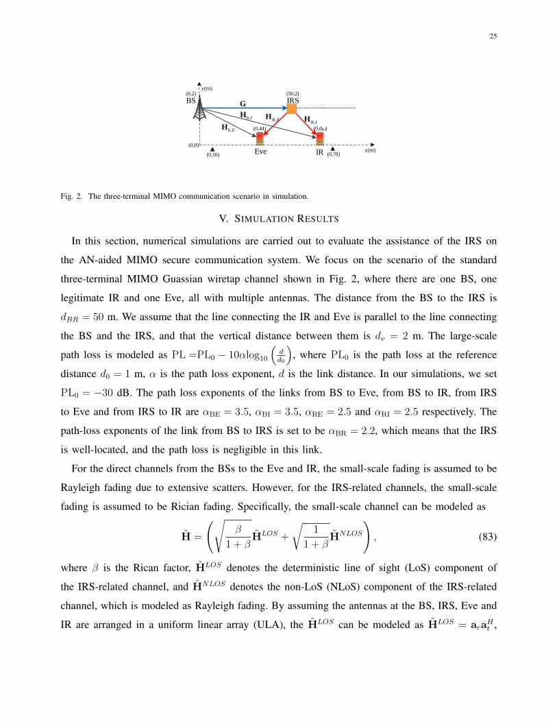
Fig. 2. The three-terminal MIMO communication scenario in simulation.

V. SIMULATION RESULTS

In this section, numerical simulations are carried out to evaluate the assistance of the IRS on

the AN-aided MIMO secure communication system. We focus on the scenario of the standard

three-terminal MIMO Guassian wiretap channel shown in Fig. 2, where there are one BS, one

legitimate IR and one Eve, all with multiple antennas. The distance from the BS to the IRS is

dBR = 50 m. We assume that the line connecting the IR and Eve is parallel to the line connecting

the BS and the IRS, and that the vertical distance between them is dv = 2 m. The large-scale

path loss is modeled as PL =PL0 − 10αlog10

(dd0

), where PL0 is the path loss at the reference

distance d0 = 1 m, α is the path loss exponent, d is the link distance. In our simulations, we set

PL0 = −30 dB. The path loss exponents of the links from BS to Eve, from BS to IR, from IRS

to Eve and from IRS to IR are αBE = 3.5, αBI = 3.5, αRE = 2.5 and αRI = 2.5 respectively. The

path-loss exponents of the link from BS to IRS is set to be αBR = 2.2, which means that the IRS

is well-located, and the path loss is negligible in this link.

For the direct channels from the BSs to the Eve and IR, the small-scale fading is assumed to be

Rayleigh fading due to extensive scatters. However, for the IRS-related channels, the small-scale

fading is assumed to be Rician fading. Specifically, the small-scale channel can be modeled as

H =

(√β

1 + βHLOS +

√1

1 + βHNLOS

), (83)

where β is the Rican factor, HLOS denotes the deterministic line of sight (LoS) component of

the IRS-related channel, and HNLOS denotes the non-LoS (NLoS) component of the IRS-related

channel, which is modeled as Rayleigh fading. By assuming the antennas at the BS, IRS, Eve and

IR are arranged in a uniform linear array (ULA), the HLOS can be modeled as HLOS = araHt ,

26

where at and ar are the steering vectors of the transmitting and receiving arrays respectively. The

at and ar are defined as,

at =[

1, exp(j2π dtλ

sinϕt), · · · , exp(j2π dtλ

(Nt − 1) sinϕt)]T, (84a)

ar =[

1, exp(j2π drλ

sinϕr), · · · , exp(j2π drλ

(Nr − 1) sinϕr)]T. (84b)

In (84), λ is the wavelength; dt and dr are the element intervals of the transmitting and receiving

array; ϕt and ϕr are the angle of departure and the angle of arrival; Nt and Nr are the number

of antennas/elements at the transmitter and receiver, respectively. We set dtλ

= drλ

= 0.5, and

ϕt = tan−1( yr−ytxr−xt ), ϕr = π − ϕt, where (xt, yt) is the location of the transmitter, and (xr, yr) is

the location of the receiver.

If not specified, the simulation parameters are set as follows. The IR’s noise power and the Eve’s

noise power are σ2I = −75 dBm and σ2

E = −75 dBm. The numbers of BS antennas, IR antennas,

and Eve antennas are NT = 4, NI = 2, and NE = 2 respectively. There are d = 2 data streams

and M = 50 IRS reflection elements. The transmit power limit is PT = 15 dBm, and the error

tolerance is ε = 10−6. The horizontal distance between the BS and the Eve is dBE = 44 m. The

horizontal distance between the BS and the IR is selected from dBI = [10 m, 70 m]. The channels

are realized 200 times independently to average the simulation results.

A. Convergence Analysis

The convergence performance of the proposed BCD-MM algorithm is investigated. The iterations

of the BCD algorithm are termed as outer-layer iterations, while the iterations of the MM algorithm

are termed as the inner-layer iterations. Fig. 3 shows three examples of convergence behaviour for

M =10, 20 and 40 phase shifts of IRS. In Fig. 3, the SR increases versus the iteration number,

and finally reaches a stable value. It is shown that the algorithm converges quickly, almost with

20 iterations, which demonstrates the efficiency of the proposed algorithm. Moreover, a larger

converged SR value is reached with a larger M , which means that better security can be obtained

by using more IRS elements. However, more IRS elements bring a heavier computation, which is

demonstrated in Fig. 3 in the form of a slower convergence speed with more phase shifters.

Specifically, we evaluate the convergence performance of the MM algorithm used for solving

the optimal IRS phase shifts. The inner-layer iterative process of the MM algorithm in the first

iteration of the BCD algorithm is shown in Fig. 4. The SR value increases as the iteration number

increases, and finally converges to a stable value. According with the convergency performance

27

0 5 10 15 20 25 30 35 40 45 504

4.5

5

5.5

6

6.5

7

Number of Outer−layer Iterations

SR

(bi

t/s/H

z)

M=10M=20M=40

Fig. 3. Convergence behaviour of the BCD algorithm.

0 200 400 600 800 10004.35

4.4

4.45

4.5

4.55

4.6

4.65

Number of Inner−layer Iterations

SR

(bi

t/s/H

z)

M=10M=20M=40

Fig. 4. Convergence behaviour of the MM algorithm.

in the out-layer iteration, similar conclusions can be drawn for the inner-layer iteration, which is

that a higher converged SR value can be obtained with more phase shifts but at the cost of lower

convergence speed. The reason for the lower convergence speed with larger M value is that more

optimization variables are introduced, which require more computation complexity.

B. Performance Evaluation

In this subsection, our proposed algorithm is evaluated by comparing the simulation results to

three schemes of

1) RandPhase: The phase shifts of the IRS are randomly selected from [0, 2π]. In this scheme,

the MM algorithm is skipped, and only the TPC matrix and AN covariance matrix are

optimized.

2) No-IRS: Without the IRS, the channel matrices of IRS related links become zero matrices,

which is HR,I = 0, HR,E = 0 and G = 0. This scheme results a conventional AN-aided

communication system, and only the TPC matrix and AN covariance matrix need to be

optimized.

3) BCD-QCQP-SDR: The BCD algorithm is utilized. However, the TPC matrix and the AN

covariance matrix is optimized by tackling Problem (30) as a QCQP problem, which is solved

by the general CVX solvers, e.g. Sedumi or Mosek. The phase shifts of IRS are optimized

by solving Problem (59) with the SDR technique.

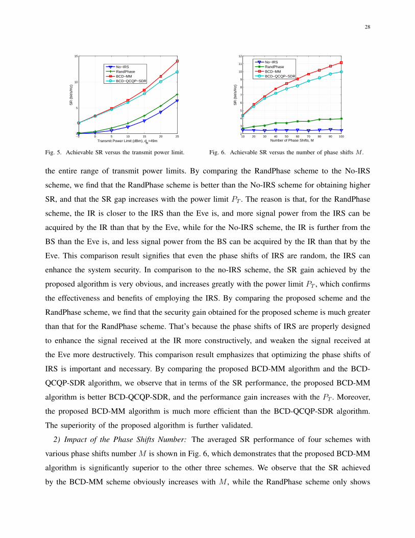
1) Impact of Transmit Power: To evaluate the impact of the transmit power limit PT , the average

SRs versus the transmit power limit for various schemes are given in Fig. 5, which demonstrates

that the achieved SRs of three schemes increase as the power limit PT increases. It is observed

that the BCD-MM algorithm significantly outperforms the other three benchmark schemes over

28

−5 0 5 10 15 20 250

5

10

15

Transmit Power Limit (dBm), dBI

=49m

SR

(bi

t/s/H

z)

No−IRSRandPhaseBCD−MMBCD−QCQP−SDR

Fig. 5. Achievable SR versus the transmit power limit.

10 20 30 40 50 60 70 80 90 1002

3

4

5

6

7

8

9

10

11

12

Number of Phase Shifts, M

SR

(bi

t/s/H

z)


Fig. 6. Achievable SR versus the number of phase shifts M .

the entire range of transmit power limits. By comparing the RandPhase scheme to the No-IRS

scheme, we find that the RandPhase scheme is better than the No-IRS scheme for obtaining higher

SR, and that the SR gap increases with the power limit PT . The reason is that, for the RandPhase

scheme, the IR is closer to the IRS than the Eve is, and more signal power from the IRS can be

acquired by the IR than that by the Eve, while for the No-IRS scheme, the IR is further from the

BS than the Eve is, and less signal power from the BS can be acquired by the IR than that by the

Eve. This comparison result signifies that even the phase shifts of IRS are random, the IRS can

enhance the system security. In comparison to the no-IRS scheme, the SR gain achieved by the

proposed algorithm is very obvious, and increases greatly with the power limit PT , which confirms

the effectiveness and benefits of employing the IRS. By comparing the proposed scheme and the

RandPhase scheme, we find that the security gain obtained for the proposed scheme is much greater

than that for the RandPhase scheme. That’s because the phase shifts of IRS are properly designed

to enhance the signal received at the IR more constructively, and weaken the signal received at

the Eve more destructively. This comparison result emphasizes that optimizing the phase shifts of

IRS is important and necessary. By comparing the proposed BCD-MM algorithm and the BCD-

QCQP-SDR algorithm, we observe that in terms of the SR performance, the proposed BCD-MM

algorithm is better BCD-QCQP-SDR, and the performance gain increases with the PT . Moreover,

the proposed BCD-MM algorithm is much more efficient than the BCD-QCQP-SDR algorithm.

The superiority of the proposed algorithm is further validated.

2) Impact of the Phase Shifts Number: The averaged SR performance of four schemes with

various phase shifts number M is shown in Fig. 6, which demonstrates that the proposed BCD-MM

algorithm is significantly superior to the other three schemes. We observe that the SR achieved

by the BCD-MM scheme obviously increases with M , while the RandPhase scheme only shows

29

10 20 30 40 50 60 700

2

4

6

8

10

12

14

16

18

BS−IR Horizontal Distance, dBI

(m)

SR

(bi

t/s/H

z)


Fig. 7. Achievable SR versus the location of the IR dBI.

2 2.2 2.4 2.6 2.8 3 3.2 3.4 3.62

3

4

5

6

7

8

9

10

11

α IRS

SR

(bi

t/s/H

z)


Fig. 8. Achievable SR versus the path loss exponent of IRS-

related links.

a slight improvement as M increases, and the No-IRS scheme has very low SRs irrelative with

M . Larger the element number M of IRS is, more significant the performance gain obtained by

the proposed algorithm is. For example, when M is small as M = 10, the SR gain of the BCD-

MM relative to the No-IRS is only 1.3 bit/s/Hz, while this SR gain becomes 9.5 bit/s/Hz when

M increases to M = 100. The performance gain for the proposed algorithm originates from two

perspectives. On the one hand, a higher array gain can be obtained by increasing M , since more

signal power can be received at the IRS with larger M . On the other hand, a higher reflecting

beamforming gain can be obtained by increasing M , which means that the sum of coherently

adding the reflected signals at the IRS elements increases with M by appropriately designing the

phase shifts. However, only the array gain can be exploited by the RandPhase scheme, thus the SRs

for it increase very slowly, and remain at much lower values than those for the proposed algorithm.

These results further confirm that more security improvements can be archived by using a large IRS

with more reflect elements and optimizing the phase shifts properly, however there may bring the

computation complexity problem. In comparison to the BCD-QCQP-SDR algorithm, the proposed

BCD-MM algorithm can achieve the higher SR, and the SR performance gap increases with M .

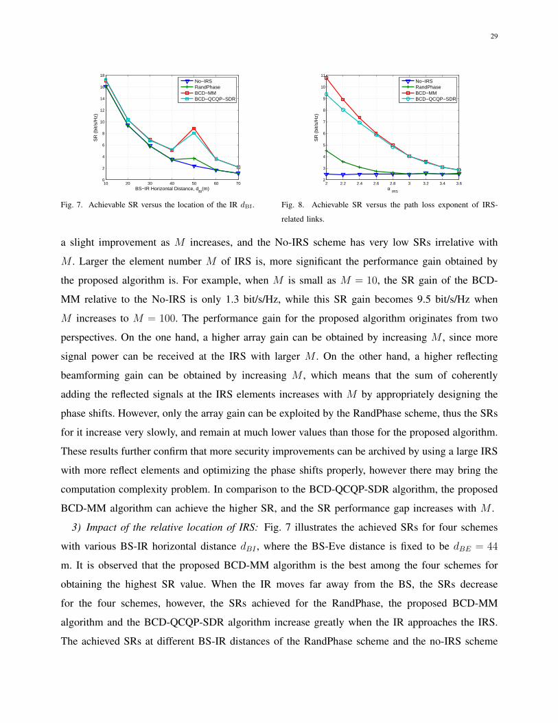
3) Impact of the relative location of IRS: Fig. 7 illustrates the achieved SRs for four schemes

with various BS-IR horizontal distance dBI , where the BS-Eve distance is fixed to be dBE = 44

m. It is observed that the proposed BCD-MM algorithm is the best among the four schemes for

obtaining the highest SR value. When the IR moves far away from the BS, the SRs decrease

for the four schemes, however, the SRs achieved for the RandPhase, the proposed BCD-MM

algorithm and the BCD-QCQP-SDR algorithm increase greatly when the IR approaches the IRS.

The achieved SRs at different BS-IR distances of the RandPhase scheme and the no-IRS scheme

30

are almost the same, except for dBI ∈ [40m, 50m], in which case the IRS brings a prominent

security enhancement when IR becomes close to it even with random IRS phase shifts. Similarly,

the proposed BCD-MM algorithm and the BCD-QCQP-SDR algorithm can achieve almost the same

SRs, except for dBI ∈ [40m, 50m], in which case the IR is close to the IRS, and the proposed

BCD-MM algorithm is superior to the BCD-QCQP-SDR algorithm. For other BS-IR distances

where the IR is far from the IRS, the SRs of RandPhase scheme are similar with those of the

No-IRS scheme due to the not fully explored potential of IRS. By optimizing the phase shifts

of IRS, the SRs are enhanced at different BS-IRS distances. And the SR gain of the proposed

BCD-MM algorithm over the RandPhase scheme increases when the IR moves close to the IRS

(dBI ∈ [40m, 50m]). This signifies that as long as the IRS is deployed close to the IR, significant

security enhancement can be achieved by the IRS in an AN-aided MIMO communication system.

Moreover, it is highly recommended that the IRS phase shifts should be optimized to prevent the

system security degrading into the level of No-IRS scheme.

4) Impact of the Path Loss Exponent of IRS-related Links: In the above simulations, the path

loss exponents of the IRS-related links (including the BS-IRS link, IRS-IR link and IRS-Eve link)

are set to be low by assuming that the IRS is properly located to obtain clean channels without

heavy blockage. Practically, such kind of settings may not always be sensible due to the real-

field environment. Thus, it is necessary to investigate the security gain brought by the IRS and our

proposed algorithm with higher values of IRS-related path loss exponents. For the sake of analysis,

we assume the path-loss exponents of the links from BS to IRS, from IRS to IR and from IRS

to Eve are the same as αBR = αRI = αRE∆= αIRS. Then, the achieved SRs versus the path-loss

exponent αIRS of IRS-related links are shown in Fig. 8, which demonstrates that the SR obtained

by the BCD-MM algorithm decreases as αIRS increases, and finally drops to the same SR value

which is achieved by the RandPhase, BCD-QCQP-SDR and No-IRS schemes. The reason is that

larger αIRS means more severe signal attenuation in the IRS-related links, and more weakened

signal received and reflected at the IRS. In comparison to the BCD-QCQP-SDR algorithm, the

proposed BCD-MM algorithm can achieve the higher SR when the channel state of the IRS related

channels is good, i.e., αIRS is low, and achieve almost the same SR when αIRS is large. Similarly,

the performance gains brought by our proposed algorithm over the RandPhase and No-IRS schemes

is significant with a small αIRS. Specifically, for αIRS = 2 (almost ideal channels), the security

gain is up to 9.6 bit/s/Hz over the No-IRS scheme, and 6.8 bit/s/Hz over the RandPhase scheme.

31

−5 0 5 10 15 20 250

5

10

15

20

25

30

Transmit Power Limit (dB), dBI

=49m, dBE

=60m

SR

(bi

t/s/H

z)

d=1,NI=N

E=4

d=2,NI=N

E=4

d=3,NI=N

E=4

d=4,NI=N

E=4

d=1,NI=N

E=1

Fig. 9. Achievable SR versus the transmit power limit for various

numbers of data streams.

0.2 0.3 0.4 0.5 0.6 0.7 0.8 0.9 11

2

3

4

5

6

7

Reflection Amplitude, η

SR

(bi

t/s/H

z)


Fig. 10. Achievable SR versus the reflection amplitude η.

Therefore, the security gain of IRS-assisted systems depends on the channel conditions of the

IRS-related links. This suggests that it is much preferred to deploy the IRS with fewer obstacles,

in which case, the performance gain brought by the IRS can be explored thoroughly. Fig. 8 also

shows that when αIRS is small, the RandPhase scheme can obtain security gain over the No-IRS

scheme, but this security gain decreases to zero when αIRS becomes large. However, the SR gain

of the RandPhase scheme over the No-IRS scheme is almost negligible in comparison to the SR

gain of the proposed scheme over the No-IRS scheme, which demonstrates that the necessity of

jointly optimizing the TPC matrix, AN covariance matrix and the phase shifts at the IRS.

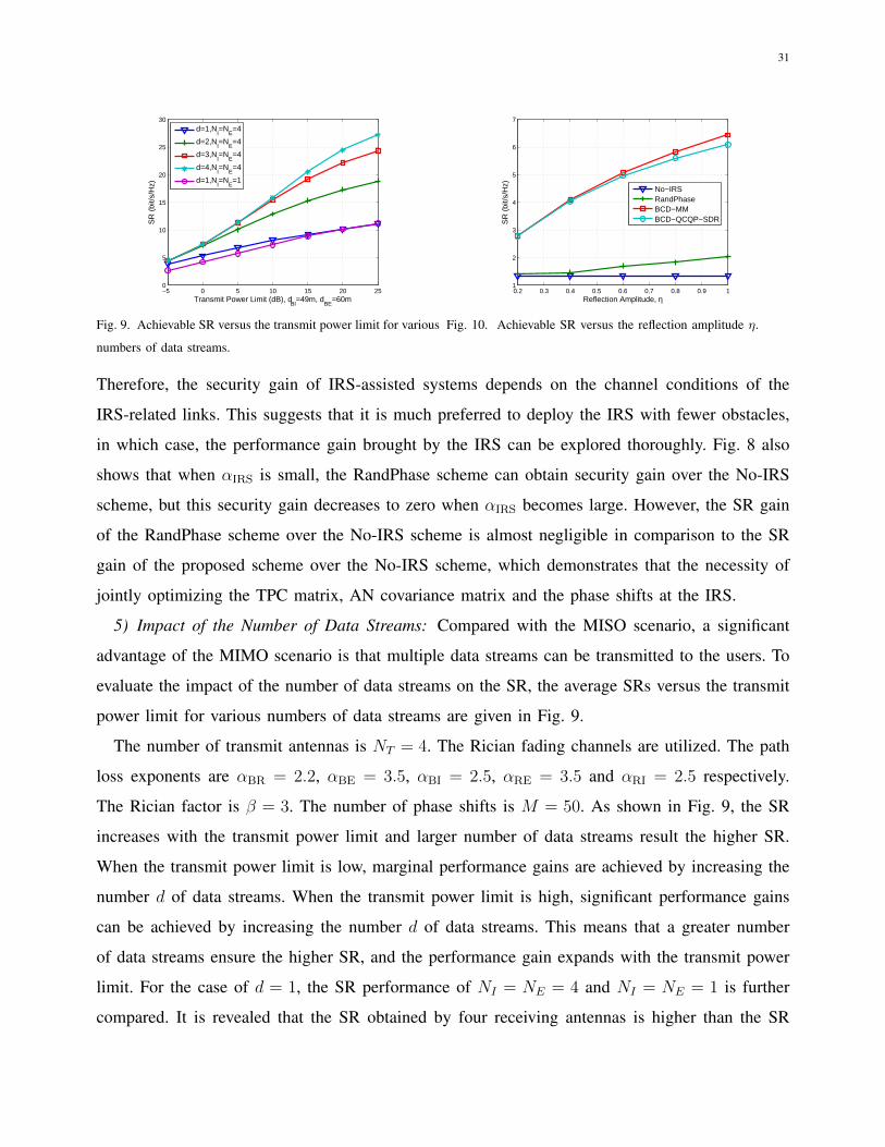
5) Impact of the Number of Data Streams: Compared with the MISO scenario, a significant

advantage of the MIMO scenario is that multiple data streams can be transmitted to the users. To

evaluate the impact of the number of data streams on the SR, the average SRs versus the transmit

power limit for various numbers of data streams are given in Fig. 9.

The number of transmit antennas is NT = 4. The Rician fading channels are utilized. The path

loss exponents are αBR = 2.2, αBE = 3.5, αBI = 2.5, αRE = 3.5 and αRI = 2.5 respectively.

The Rician factor is β = 3. The number of phase shifts is M = 50. As shown in Fig. 9, the SR

increases with the transmit power limit and larger number of data streams result the higher SR.

When the transmit power limit is low, marginal performance gains are achieved by increasing the

number d of data streams. When the transmit power limit is high, significant performance gains

can be achieved by increasing the number d of data streams. This means that a greater number

of data streams ensure the higher SR, and the performance gain expands with the transmit power

limit. For the case of d = 1, the SR performance of NI = NE = 4 and NI = NE = 1 is further

compared. It is revealed that the SR obtained by four receiving antennas is higher than the SR

32

obtained by one single receiving antenna when the transmit power limit is relatively low. With the

increase of transmit power limit, the SR performance gain brought by multiple receiving antennas

decreases. When the transmit power limit is high enough, the SR performance is saturated, and

the SR performance of the multiple receiving antennas and single receiving antenna becomes the

same.

6) Impact of the Reflection Amplitude: Due to the manufactural and hardware reasons, the

signals reflected by the IRS may be attenuated. Then, in Fig. 10, we study the impact of the

reflection amplitude on the security performance. The transmit power limit is 10dBm. We assume

that the reflection amplitudes of all the IRS elements are same as η, and that the phase shift matrix

of the IRS is rewritten as Φ = ηdiag{φ1, · · · , φm, · · · , φM}. As expected, the SR achieved by the

IRS-aided scheme increases with η due to less power loss. As η increases, the superiority of the

proposed BCD-MM algorithm over the other algorithms becomes more obvious. The reflection

amplitude has a great impact on the security performance. Specifically, when η increases from 0.2

to 1, the SR increases over 3.6 bit/s/Hz for the proposed BCD-MM algorithm.

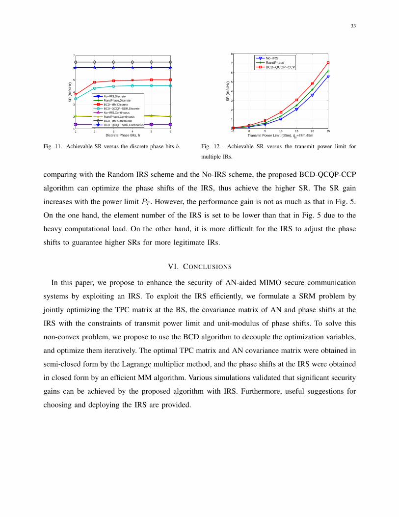
7) Impact of the Discrete Phase Shifts: In practice, it is difficult to realize continuous phase

shifts at the reflecting elements of the IRS due to the high manufacturing cost. It is more cost-

effective to implement only discrete phase shifts with a small number of control bits for each

element, e.g., 1-bit for two-level (0 or π) phase shifts. Thus, the impact of the controlling bits b of

the discrete phase shifts on the security performance is investigated in Fig. 11. The transmit power

limit is 10dBm. It is shown that the SR with continuous phase shifts of the IRS is higher than

those with discrete phase shifts. The limited discrete phase shifts inevitably cause SR performance

degradation. The SR of the IRS with discrete phase shifts increases with the number of controlling

bits b, and becomes saturated when b ≥ 4, which means that the SR loss is inevitable even when

the number of controlling bits b is high. For the proposed BCD-MM algorithm, the maximum SR

gap between the continuous phase shifts and the discrete phase shifts is 1.4 bit/s/Hz.

8) Multiple IRs Scenario: Finally, we consider the multiple IRs scenario to investigate the

security enhancement brought by the IRS on the AN-aided MIMO communication systems. The

horizontal distances between the BS and the two IRs are selected as dBI,1 = 47m and dBI,2 = 49m.

Considering the heavy computational load, the element number of the IRS is assumed to be

M = 20. The proposed BCD-QCQP-CCP algorithm is utilized to perform the joint optimization

of the TPC matrix, AN covariance matrix and the phase shifts of the IRS. The achieved SRs for

the proposed algorithm, the random IRS scheme and the No-IRS scheme are shown in Fig. 12. By

33

1 2 3 4 5 61

2

3

4

5

6

7

Discrete Phase Bits, b

SR

(bi

t/s/H

z)

No−IRS,DiscreteRandPhase,DiscreteBCD−MM,DiscreteBCD−QCQP−SDR,DiscreteNo−IRS,ContinuousRandPhase,ContinuousBCD−MM,ContinuousBCD−QCQP−SDR,Continuous

Fig. 11. Achievable SR versus the discrete phase bits b.

−5 0 5 10 15 20 250

1

2

3

4

5

6

7

8

Transmit Power Limit (dBm), dBI

=47m,49m

SR

(bi

t/s/H

z)

No−IRSRandPhaseBCD−QCQP−CCP

Fig. 12. Achievable SR versus the transmit power limit for

multiple IRs.

comparing with the Random IRS scheme and the No-IRS scheme, the proposed BCD-QCQP-CCP

algorithm can optimize the phase shifts of the IRS, thus achieve the higher SR. The SR gain

increases with the power limit PT . However, the performance gain is not as much as that in Fig. 5.

On the one hand, the element number of the IRS is set to be lower than that in Fig. 5 due to the

heavy computational load. On the other hand, it is more difficult for the IRS to adjust the phase

shifts to guarantee higher SRs for more legitimate IRs.

VI. CONCLUSIONS

In this paper, we propose to enhance the security of AN-aided MIMO secure communication

systems by exploiting an IRS. To exploit the IRS efficiently, we formulate a SRM problem by

jointly optimizing the TPC matrix at the BS, the covariance matrix of AN and phase shifts at the

IRS with the constraints of transmit power limit and unit-modulus of phase shifts. To solve this

non-convex problem, we propose to use the BCD algorithm to decouple the optimization variables,

and optimize them iteratively. The optimal TPC matrix and AN covariance matrix were obtained in

semi-closed form by the Lagrange multiplier method, and the phase shifts at the IRS were obtained

in closed form by an efficient MM algorithm. Various simulations validated that significant security

gains can be achieved by the proposed algorithm with IRS. Furthermore, useful suggestions for

choosing and deploying the IRS are provided.

34

APPENDIX A

DERIVATION OF THE PROBLEM (27)

By substituting h1(UI ,V,VE,WI) of (13), h2(UE,VE,WE) of (17) and h3(V,VE,WX) of

(21) into (25), we have

ClAN(UI ,WI ,UE,WE,WX ,V,VE,Φ) = log |WI | − Tr(WIEI(UI ,V,VE)) + log |WE|

− Tr(WEEE(UE,VE)) + log |WX | − Tr(WXEX(V,VE)) + d+Nt +NE

= Cg0 − Tr(WIEI(UI ,V,VE))︸︷︷︸g1

− Tr(WEEE(UE,VE))︸︷︷︸g2

− Tr(WXEX(V,VE))︸︷︷︸g3

, (85)

where Cg0∆= log |WI |+ log |WE|+ log |WX |+ d+Nt +NE .

Cg0 contains the constant terms irrelated with V,VE,Φ. By putting matrix functions EI , EE

and EX into (85), we expand g1, g2, and g3 respectively as follows.

(1) g1 can be reformulated as

g1 = Tr(WI [(I−UIHHIV)(I−UI

HHIV)H

+ UIH(HIVEVE

HHHI + σ2

IINI)UI ])

= Tr(WI [(I−VHHHI UI −UI

HHIV + UIHHIVVHHH

I UI)

+ (UIHHIVEVE

HHHI UI+UI

Hσ2IINI

UI)]). (86)

By gathering the constant terms related with WI ,UI in Cg1 , g1 can be simplified as

g1 = −Tr(WIVHHH

I UI)− Tr(WIUIHHIV) + Tr(VHHH

I UIWIUIHHIV)

+ Tr(VEHHH

I UIWIUIHHIVE) + Cg1 , (87)

where Cg1∆= Tr(WI + σ2

IWIUIHUI).


g2 = Tr(WE[(I−UEHHEVE)(I−UE

HHEVE)H

+ σ2EUE

HUE])

= Tr(WE[(I−VEHHH

EUE −UEHHEVE + UE

HHEVEVEHHH

EUE

+ σ2EUE

HUE]). (88)

By gathering the constant terms related with WE,UE in Cg2 , g2 can be simplified as

g2 = −Tr(WEVEHHH


HHHEUEWEUE

HHEVE) + Cg2 ,

(89)

35

where Cg2∆= Tr(WE + σ2

EWEUEHUE).


g3 = Tr(WX(INE+ σ−2

E HE(VVH + VEVEH)HH

E )). (90)

By gathering the constant terms related with WX in Cg3 , g3 can be simplified as

g3 = σ−2E Tr(VHHH

EWXHEV) + σ−2E Tr(VE

HHHEWXHEVE) + Cg3 , (91)

where Cg3∆= Tr(WX).

By substituting (87), (89) and (91) into (85), we have

ClAN(UI ,WI ,UE,WE,WX ,V,VE,Φ) = Tr(WIV

HHHI UI) + Tr(WIUI

HHIV)

− Tr(VHHHI UIWIUI

HHIV)− Tr(VEHHH

I UIWIUIHHIVE) + Tr(WEVE

HHHEUE)

+ Tr(WEUEHHEVE)− Tr(VE

HHHEUEWEUE

HHEVE)− σ−2E Tr(VHHH

EWXHEV)

− σ−2E Tr(VE

HHHEWXHEVE) + Cg, (92)

where Cg∆= Cg0 − Cg1 − Cg2 − Cg3 .

Equation (92) can be rewritten more compactly as

ClAN(UI ,WI ,UE,WE,WX ,V,VE,Φ) = Cg + Tr(WIV

HHHI UI) + Tr(WIUI

HHIV)

− Tr(VHHV V) + Tr(WEVEHHH

EUE) + Tr(WEUEHHEVE)− Tr(VE

HHV EVE). (93)

where

HV = HHI UIWIUI

HHI + σ−2E HH

EWXHE. (94)

HV E = HHI UIWIUI

HHI + HHEUEWEUE

HHE + σ−2E HH

EWXHE. (95)

By substituting (93) into Problem (26), and removing the constant term Cg, we arrive at the Problem

(27).

APPENDIX B

DERIVATION OF THE NEW OF FORM IN (55)

The objective function of Problem (54) is

g0(V,VE,Φ) =− Tr(WIVHHH

I UI)− Tr(WIUIHHIV) + Tr(VHHV V)

− Tr(WEVEHHH


HHV EVE). (96)

36

The third term of (96) is

Tr(VHHV V

)= Tr

[VH

(HHI UIWIU

HI HI + σ−2

E HHEWXHE

)V]

= Tr[HIVVHHH

I UIWIUHI

]+ σ−2

E Tr[HEVVHHH

EWX

]. (97)

The sixth term of (96) is

Tr(VHEHV EVE

)=Tr

[VHE

(HHI UIWIU

HI HI + HH


E HHEWXHE

)VE

]=Tr

[HIVEVH

E HHI UIWIU

HI

]+ Tr

[HEVEVH

E HHEUEWEUH

E

]+ σ−2

E Tr[HEVEVH

E HHEWX

]. (98)

The summation of Equation (97) and Equation (98) is

Tr(VHHV V

)+ Tr

(VHEHV EVE

)=Tr

[HI

(VVH + VEVH

E

)HHI UIWIU

HI

]+ σ−2

E Tr[HE

(VVH + VEVH

E

)HHEWX

]+ Tr

[HEVEVH

E HHEUEWEUH

E

]. (99)

By defining VX =(VVH + VEVH

E

)and MI = UIWIU

HI , the first part of (99) can be derived

as

Tr[HI

(VVH + VEVH

E

)HHI UIWIU

HI

]= Tr

[HIVXHH

I MI

]= Tr

[(Hb,I + HR,IΦG) VX

(HHb,I + GHΦHHH

R,I

)MI

]= Tr

[(Hb,IVXHH

b,I + Hb,IVXGHΦHHHR,I + HR,IΦGVXHH

b,I + HR,IΦGVXGHΦHHHR,I

)MI

]= Tr[Hb,IVXHH

b,IMI + Hb,IVXGHΦHHHR,IMI + HR,IΦGVXHH

b,IMI

+ HR,IΦGVXGHΦHHHR,IMI ]. (100)

The derivation in (100) can be used for the second and third parts of (99).

Based on the derivation in (100), it is obvious that the second part of (99) can be derived as

σ−2E Tr

[HE

(VVH + VEVH

E

)HHEWX

]= σ−2

E Tr[Hb,EVXHHb,EWX + Hb,EVXGHΦHHH

R,EWX + HR,EΦGVXHHb,EWX

+ HR,EΦGVXGHΦHHHR,EWX ]. (101)

37

Based on the derivation in (100) and by defining ME = UEWEUHE , it is obvious that the third

part of (99) can be derived as

Tr[HEVEVH

E HHEUEWEUH

E

]= Tr

[HE

(VEVH

E

)HHEME

]= Tr[Hb,EVEVH

EHHb,EME + Hb,EVEVH

EGHΦHHHR,EME + HR,EΦGVEVH

EHHb,EME

+ HR,EΦGVEVHEGHΦHHH

R,EME]. (102)

By adding (100), (101) and (102), and gathering constant terms irreverent with Φ, Equation (99)

becomes

Tr(VHHV V

)+ Tr

(VHEHV EVE

)= Tr

[ΦH

(HHR,IMIHb,IVXGH + σ−2

E HHR,EWXHb,EVXGH + HH

R,EMEHb,EVEVHEGH

)]+ Tr

[Φ(GVXHH

b,IMIHR,I + σ−2E GVXHH

b,EWXHR,E + GVEVHEHH

b,EMEHR,E

)]+ Tr

[ΦGVXGHΦH

(HHR,IMIHR,I + σ−2

E HHR,EWXHR,E

)]+ Tr

[ΦGVEVH

EGHΦHHHR,EMEHR,E

]+ Ct1 , (103)

where

Ct1 = Tr[Hb,IVXHH

b,IMI

]+ σ−2

E Tr[Hb,EVXHH

b,EWX

]+ Tr

[Hb,EVEVH

EHHb,EME

]. (104)

The first term of g0(V,VE,Φ) is derived as

Tr(WIV

HHHI UI

)=Tr

(UIW

HI VHHH

I

)=Tr

[UIW

HI VHHH

b,I

]︸︷︷︸Ct2 (constant for Φ)

+Tr[HHR,IUIW

HI VHGHΦH

].

(105)

The second term of g0(V,VE,Φ) is derived as

Tr(WIU

HI HIV

)= Tr

(HIVWIU

HI

)= Tr

[(Hb,I + HR,IΦG) VWIU

HI

]= Tr

[Hb,IVWIU

HI


+Tr[ΦGVWIU

HI HR,I

]. (106)

The fourth term of g0(V,VE,Φ) is derived as

Tr(WEVH

E HHEUE

)= Tr

(UEWH

EVHE HH

E

)= Tr

[UEWH

EVHEHH

b,E


+Tr[HHR,EUEWH

EVHEGHΦH

]. (107)

38

The fifth term of g0(V,VE,Φ) is derived as

Tr(WEUH

E HEVE

)= Tr

(HEVEWEUH

E

)= Tr

[Hb,EVEWEUH

E


+Tr[ΦGVEWEUH

EHR,E

]. (108)

By including the first term in (105), the second term in (106), the fourth term in (107), the fifth

term in (108), and the sum of the third and six terms in (103) of g0(V,VE,Φ) and gathering

constant terms irreverent with Φ, we have

g0(Φ) = −Equation (105)− Equation (106)− Equation (107)− Equation (108) + Equation (103)

= Tr

ΦH

HHR,IMIHb,IVXGH + σ−2


R,EMEHb,EVEVHEGH

−HHR,IUIW

HI VHGH −HH

R,EUEWHEVH

EGH

+ Tr

Φ

GVXHHb,IMIHR,I + σ−2

E GVXHHb,EWXHR,E + GVEVH

EHHb,EMEHR,E

−GVWIUHI HR,I −GVEWEUH

EHR,E

+ Tr

[ΦGVEVH

EGHΦH(HHR,IMIHR,I + σ−2

E HHR,EWXHR,E + HH

R,EMEHR,E

)]+ Tr

[ΦGVVHGHΦH

(HHR,IMIHR,I + σ−2

E HHR,EWXHR,E

)]+ Ct

= Tr

ΦH

HHR,IMIHb,IVXGH + σ−2


R,EMEHb,EVEVHEGH

−HHR,IUIW

HI VHGH −HH

R,EUEWHEVH

EGH

+ Tr

Φ

GVXHHb,IMIHR,I + σ−2


EHHb,EMEHR,E


EHR,E

+ Tr

[ΦGVEVH

EGHΦH(HHR,IUIWIU

HI HR,I + σ−2

E HHR,EWXHR,E + HH

R,EUEWEUHEHR,E

)]+ Tr

[ΦGVVHGHΦH

(HHR,IUIWIU

HI HR,I + σ−2

E HHR,EWXHR,E

)]+ Ct, (109)

where

Ct = Ct1 + Ct2 + Ct3 + Ct4 + Ct5 . (110)

Then g0(Φ) becomes

g0(Φ) = Tr(ΦHDH

)+ Tr (ΦD) + Tr

[ΦCV EΦHBV E

]+ Tr

(ΦCV ΦHBV

)+ Ct

= Tr(ΦHDH

)+ Tr (ΦD) + Tr

[ΦHBV EΦCV E

]+ Tr

(ΦHBV ΦCV

)+ Ct, (111)

39

where

D = GVXHHb,IMIHR,I + σ−2


EHHb,EMEHR,E


EHR,E, (112a)

CV E = GVEVHEGH , (112b)

CV = GVVHGH , (112c)

BV E =(HHR,IUIWIU

HI HR,I + σ−2

E HHR,EWXHR,E + HH

R,EUEWEUHEHR,E

), (112d)

BV =(HHR,IUIWIU

HI HR,I + σ−2

E HHR,EWXHR,E

). (112e)

REFERENCES

[1] W. Saad, M. Bennis, and M. Chen, “A vision of 6G wireless systems: Applications, trends, technologies, and open research

problems.” [Online]. Available: https://arxiv.org/abs/1902.10265

[2] Q. Wang, F. Zhou, R. Q. Hu, and Y. Qian, “Energy-efficient beamforming and cooperative jamming in IRS-assisted MISO

networks.” [Online]. Available: https://arxiv.org/abs/1911.05133

[3] W. C. Liao, T. H. Chang, W. K. Ma, and C. Y. Chi, “QoS-based transmit beamforming in the presence of eavesdroppers: An

optimized artificial-noise-aided approach,” IEEE Trans. Signal Process., vol. 59, no. 3, pp. 1202–1216, 2010.

[4] Y. Wu, A. Khisti, C. Xiao, G. Caire, K. K. Wong, and X. Gao, “A survey of physical layer security techniques for 5G wireless

networks and challenges ahead,” IEEE J. Sel. Areas Commun., vol. 36, no. 4, pp. 679–695, 2018.

[5] A. D. Wyner, “The wire-tap channel,” Bell Syst. Tech. J., vol. 54, no. 8, pp. 1355–1387, 1975.

[6] I. Csiszar and J. Korner, “Broadcast channels with confidential messages,” IEEE Trans. Inf. Theory, vol. 24, no. 3, pp.

339–348, 1978.

[7] A. Khisti and G. Wornell, “Secure transmission with multiple antennas II: The MIMOME wiretap channel.” [Online].

Available: https://arxiv.org/abs/1006.5879

[8] F. Oggier and B. Hassibi, “The secrecy capacity of the MIMO wiretap channel,” IEEE Trans. Inf. Theory, vol. 57, no. 8, pp.

4961–4972, 2011.

[9] A. Mukherjee and A. L. Swindlehurst, “Fixed-rate power allocation strategies for enhanced secrecy in MIMO wiretap

channels,” in 10th Workshop on Signal Processing Advances in Wireless Communications (SPAWC). IEEE, 2009, pp.

344–348.

[10] A. L. Swindlehurst, “Fixed SINR solutions for the MIMO wiretap channel,” in International Conference on Acoustics, Speech

and Signal Processing (ICASSP). IEEE, 2009, pp. 2437–2440.

[11] S. Goel and R. Negi, “Guaranteeing secrecy using artificial noise,” IEEE Trans. Wireless Commun., vol. 7, no. 6, pp. 2180–

2189, 2008.

[12] X. Zhou and M. R. McKay, “Secure transmission with artificial noise over fading channels: achievable rate and optimal power

allocation,” IEEE Trans. Veh. Technol., vol. 59, no. 8, pp. 3831–3842, 2010.

[13] Q. Li, M. Hong, H. T. Wai, Y. F. Liu, W. K. Ma, and Z. Q. Luo, “Transmit solutions for MIMO wiretap channels using

alternating optimization,” IEEE J. Sel. Areas Commun., vol. 31, no. 9, pp. 1714–1727, 2013.

https://arxiv.org/abs/1902.10265



40

[14] M. Di Renzo, M. Debbah, D. T. Phan Huy, A. Zappone, M. S. Alouini, C. Yuen, V. Sciancalepore, G. C. Alexandropoulos,

J. Hoydis, H. Gacanin et al., “Smart radio environments empowered by reconfigurable AI meta-surfaces: an idea whose time

has come,” EURASIP J Wirel. Comm., vol. 2019, no. 129, pp. 1–20, 2019.

[15] Q. Wu and R. Zhang, “Towards smart and reconfigurable environment: Intelligent reflecting surface aided wireless network.”

[Online]. Available: https://arxiv.org/abs/1905.00152

[16] C. Huang, S. Hu, G. C. Alexandropoulos, A. Zappone, C. Yuen, R. Zhang, M. Di Renzo, and M. Debbah,

“Holographic MIMO surfaces for 6G wireless networks: Opportunities, challenges, and trends.” [Online]. Available:


[17] Q. Wu and R. Zhang, “Beamforming optimization for wireless network aided by intelligent reflecting surface with discrete

phase shifts,” IEEE Transactions on Communications, vol. 68, no. 3, pp. 1838–1851, 2020.

[18] C. Huang, A. Zappone, G. C. Alexandropoulos, M. Debbah, and C. Yuen, “Reconfigurable intelligent surfaces for energy

efficiency in wireless communication,” IEEE Trans. Wireless Commun., vol. 18, no. 8, pp. 4157–4170, 2019.

[19] C. Huang, R. Mo, C. Yuen et al., “Reconfigurable intelligent surface assisted multiuser MISO systems exploiting deep

reinforcement learning.” [Online]. Available: https://arxiv.org/abs/2002.10072

[20] Q. Wu and R. Zhang, “Towards smart and reconfigurable environment: Intelligent reflecting surface aided wireless network,”

IEEE Communications Magazine, vol. 58, no. 1, pp. 106–112, 2020.

[21] S. Hu, F. Rusek, and O. Edfors, “Beyond massive MIMO: The potential of data transmission with large intelligent surfaces,”

IEEE Trans. Signal Process., vol. 66, no. 10, pp. 2746–2758, 2018.

[22] G. W. Ford and W. H. Weber, “Electromagnetic interactions of molecules with metal surfaces,” Phys. Rep., vol. 113, no. 4,

pp. 195–287, 1984.

[23] G. Yang, Y. C. Liang, R. Zhang, and Y. Pei, “Modulation in the air: Backscatter communication over ambient OFDM carrier,”

IEEE Trans. Commun., vol. 66, no. 3, pp. 1219–1233, 2017.

[24] R. Zhang, Y. C. Liang, C. C. Chai, and S. Cui, “Optimal beamforming for two-way multi-antenna relay channel with analogue

network coding,” IEEE J. Sel. Areas in Commun., vol. 27, no. 5, pp. 699–712, 2009.

[25] C. Pan, H. Ren, K. Wang, W. Xu, M. Elkashlan, A. Nallanathan, and L. Hanzo, “Multicell MIMO communications relying

on intelligent reflecting surface.” [Online]. Available: https://arxiv.org/abs/1907.10864

[26] X. Yu, D. Xu, and R. Schober, “MISO wireless communication systems via intelligent reflecting surfaces.” [Online].


[27] Y. Yang, B. Zheng, S. Zhang, and R. Zhang, “Intelligent reflecting surface meets OFDM: Protocol design and rate

maximization.” [Online]. Available: https://arxiv.org/abs/1906.09956

[28] Q. Wu and R. Zhang, “Intelligent reflecting surface enhanced wireless network via joint active and passive beamforming,”

IEEE Trans. Wireless Commun., vol. 18, no. 11, pp. 5394–5409, 2019.

[29] H. Guo, Y. C. Liang, J. Chen, and E. G. Larsson, “Weighted sum-rate optimization for intelligent reflecting surface enhanced

wireless networks.” [Online]. Available: https://arxiv.org/abs/1905.07920

[30] Q. U. A. Nadeem, A. Kammoun, A. Chaaban, M. Debbah, and M. S. Alouini, “Large intelligent surface assisted MIMO

communications.” [Online]. Available: https://arxiv.org/abs/1903.08127

[31] G. Zhou, C. Pan, H. Ren, K. Wang, W. Xu, and A. Nallanathan, “Intelligent reflecting surface aided multigroup multicast

MISO communication systems.” [Online]. Available: https://arxiv.org/abs/1909.04606

[32] T. Bai, C. Pan, Y. Deng, M. Elkashlan, and A. Nallanathan, “Latency minimization for intelligent reflecting surface aided

mobile edge computing.” [Online]. Available: https://arxiv.org/abs/1910.07990

[33] C. Pan, H. Ren, K. Wang, M. Elkashlan, A. Nallanathan, J. Wang, and L. Hanzo, “Intelligent reflecting











41

surface enhanced MIMO broadcasting for simultaneous wireless information and power transfer.” [Online]. Available:


[34] X. Yu, D. Xu, and R. Schober, “Enabling secure wireless communications via intelligent reflecting surfaces.” [Online].


[35] M. Cui, G. Zhang, and R. Zhang, “Secure wireless communication via intelligent reflecting surface,” IEEE Wireless Commun.

Lett., 2019.

[36] H. Shen, W. Xu, S. Gong, Z. He, and C. Zhao, “Secrecy rate maximization for intelligent reflecting surface assisted

multi-antenna communications.” [Online]. Available: https://arxiv.org/abs/1905.10075

[37] J. Chen, Y. C. Liang, Y. Pei, and H. Guo, “Intelligent reflecting surface: A programmable wireless environment for physical

layer security.” [Online]. Available: https://arxiv.org/abs/1905.03689

[38] K. Feng and X. Li, “Physical layer security enhancement exploiting intelligent reflecting surface.” [Online]. Available:


[39] Z. Luo, W. Ma, A. M. So, Y. Ye, and S. Zhang, “Semidefinite relaxation of quadratic optimization problems and applications,”

IEEE Signal Process. Mag., vol. 27, no. 3, pp. 20–34, 2010.

[40] Y. Sun, P. Babu, and D. P. Palomar, “Majorization-minimization algorithms in signal processing, communications, and machine

learning,” IEEE Trans. Signal Process., vol. 65, no. 3, pp. 794–816, 2016.

[41] P. A. Absil, R. Mahony, and R. Sepulchre, Optimization algorithms on matrix manifolds. Princeton University Press, 2009.

[42] B. Feng, Y. Wu, and M. Zheng, “Secure transmission strategy for intelligent reflecting surface enhanced wireless system,” in

2019 11th International Conference on Wireless Communications and Signal Processing (WCSP). IEEE, 2019, pp. 1–6.

[43] W. Shi, X. Zhou, L. Jia, Y. Wu, F. Shu, and J. Wang, “Enhanced secure wireless information and power transfer via

intelligent reflecting surface.” [Online]. Available: https://arxiv.org/abs/1911.01001

[44] X. Guan, Q. Wu, and R. Zhang, “Intelligent reflecting surface assisted secrecy communication via joint beamforming and

jamming.” [Online]. Available: https://arxiv.org/abs/1907.12839

[45] D. Xu, X. Yu, Y. Sun, D. W. K. Ng, and R. Schober, “Resource allocation for secure IRS-assisted multiuser MISO systems.”

[Online]. Available: https://arxiv.org/abs/1907.03085

[46] X. Tan, Z. Sun, J. M. Jornet, and D. Pados, “Increasing indoor spectrum sharing capacity using smart reflect-array,” in 2016

IEEE International Conference on Communications (ICC). IEEE, 2016, pp. 1–6.

[47] S. Hong, C. Pan, H. Ren, K. Wang, K. K. Chai, and A. Nallanathan, “Robust transmission design for

intelligent reflecting surface aided secure communication systems with imperfect cascaded CSI.” [Online]. Available:


[48] Q. Shi, W. Xu, J. Wu, E. Song, and Y. Wang, “Secure beamforming for MIMO broadcasting with wireless information and

power transfer,” IEEE Trans. Wireless Commun., vol. 14, no. 5, pp. 2841–2853, 2015.

[49] M. Grant and S. Boyd, “CVX: Matlab software for disciplined convex programming, version 2.1,” 2014.

[50] X. D. Zhang, Matrix analysis and applications. Cambridge University Press, 2017.

[51] Y. Liang, H. V. Poor et al., “Information theoretic security,” Foundations and Trends in communications and Information

Theory, vol. 5, no. 4–5, pp. 355–580, 2009.

[52] G. Zhou, C. Pan, H. Ren, K. Wang, and A. Nallanathan, “A framework of robust transmission design for IRS-aided MISO

communications with imperfect cascaded channels.” [Online]. Available: https://arxiv.org/abs/2001.07054











Artiﬁcial-Noise-Aided Secure MIMO Wireless Communications ... · This paper considers a MIMO...

Documents

Transcript of Artiﬁcial-Noise-Aided Secure MIMO Wireless Communications ... · This paper considers a MIMO...