Artificial Neural Networks: Self Organizing Networks

Artificial neural networks which are currently used in tasks such as speech and handwriting recognition are based on learning mechanisms in the brain i.esynaptic changes. In addition, one kind of artificial neural network, self organizingnetworks, is based on the topographicalorganization of the brain.

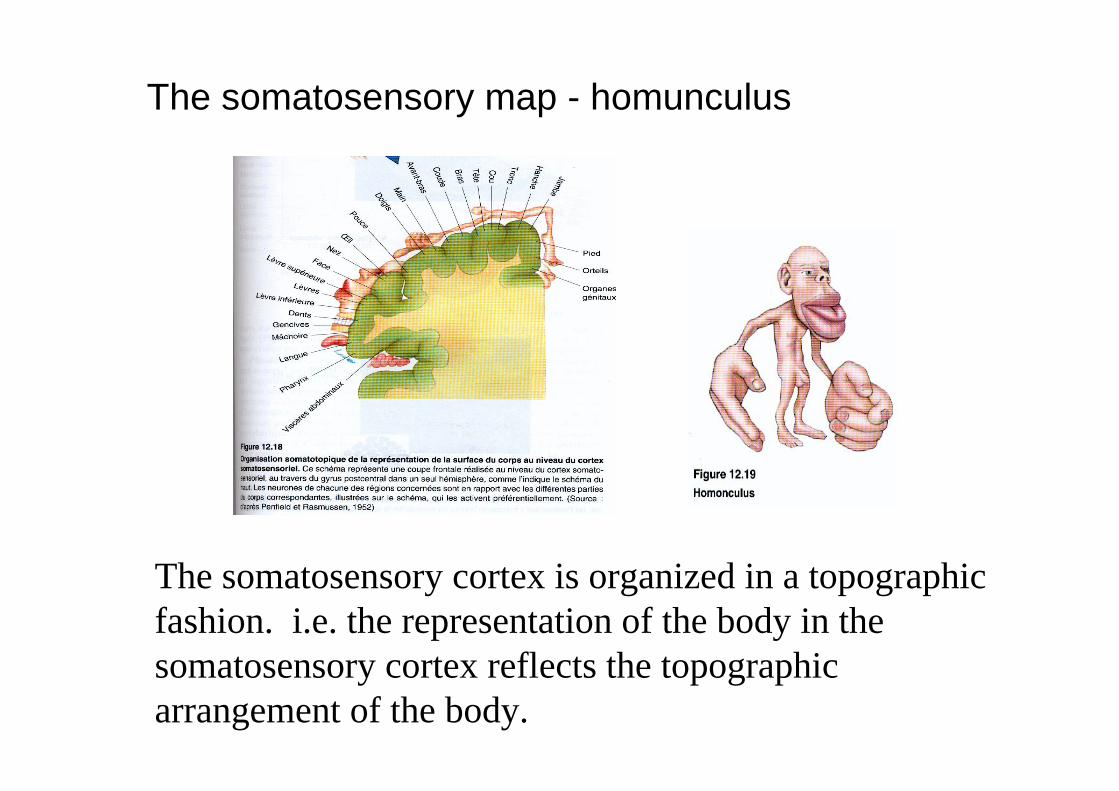
The somatosensory map - homunculus

The somatosensory cortex is organized in a topographicfashion. i.e. the representation of the body in the somatosensory cortex reflects the topographicarrangement of the body.

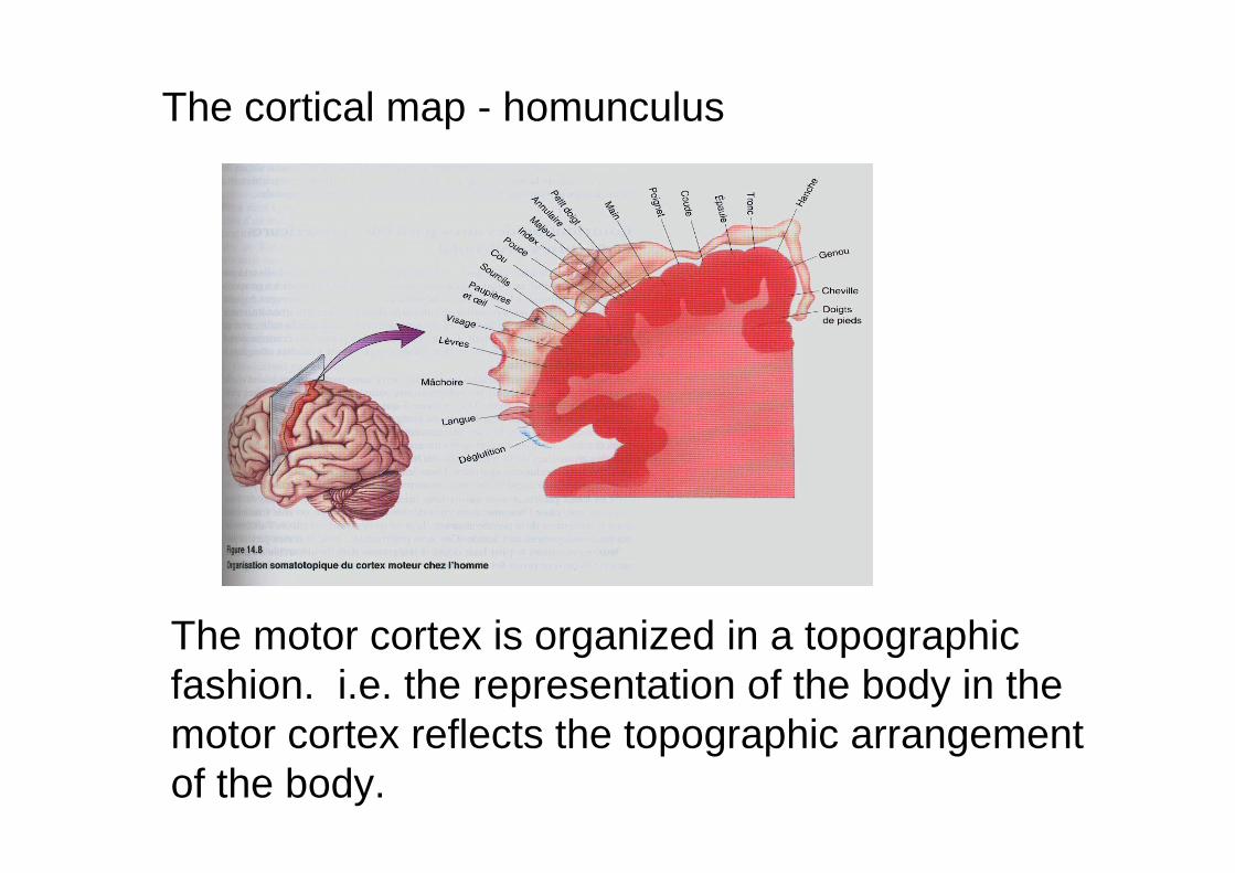
The motor cortex is organized in a topographicfashion. i.e. the representation of the body in the motor cortex reflects the topographic arrangement of the body.

The cortical map - homunculus

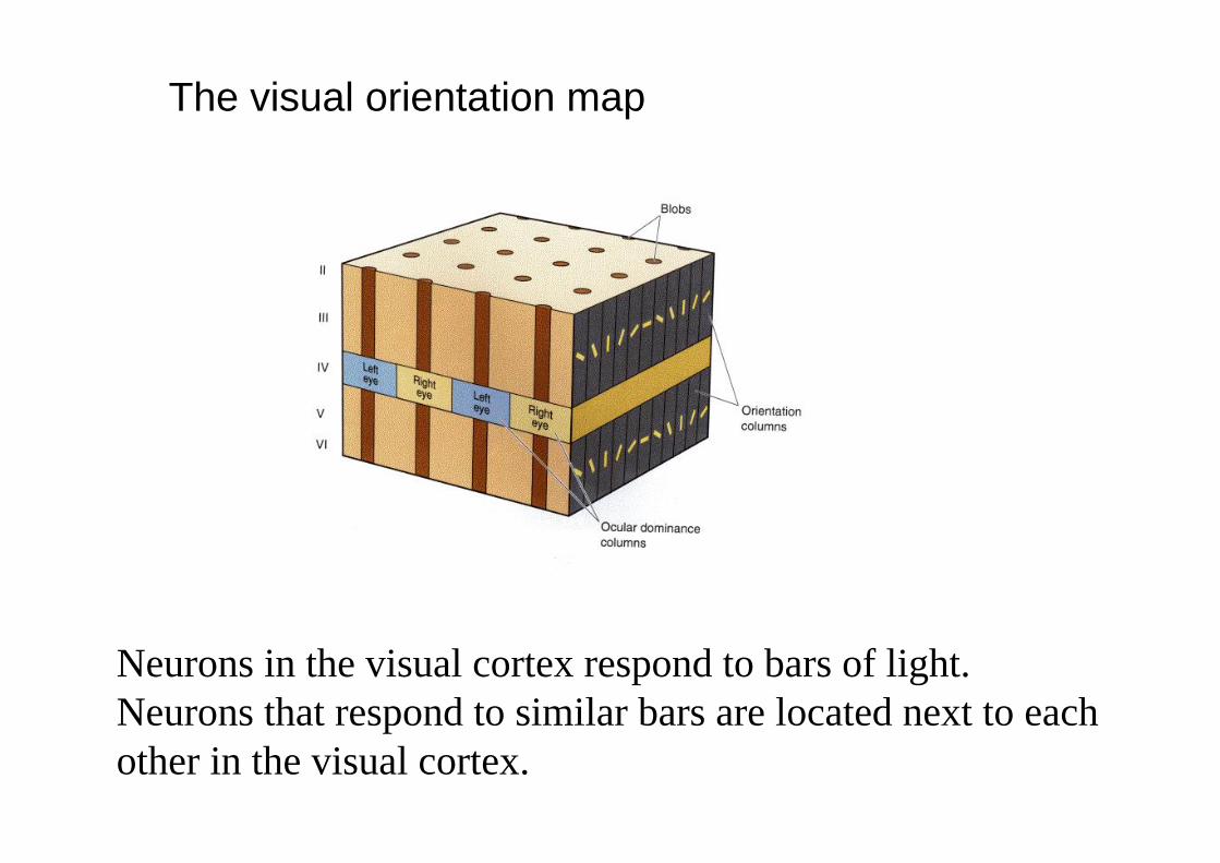
The visual orientation map

Neurons in the visual cortex respond to bars of light. Neurons that respond to similar bars are located next to eachother in the visual cortex.

Self organizing maps are based on these principles:

• Learning by changes in synaptic weight

• A topographic organization of information ie Similarinformation is found in a similar spatial location.

Self organizing maps are a type of artificial neural network. Unlike methods like back propagation, self organizing networks are unsupervised, hence the name self organizing.

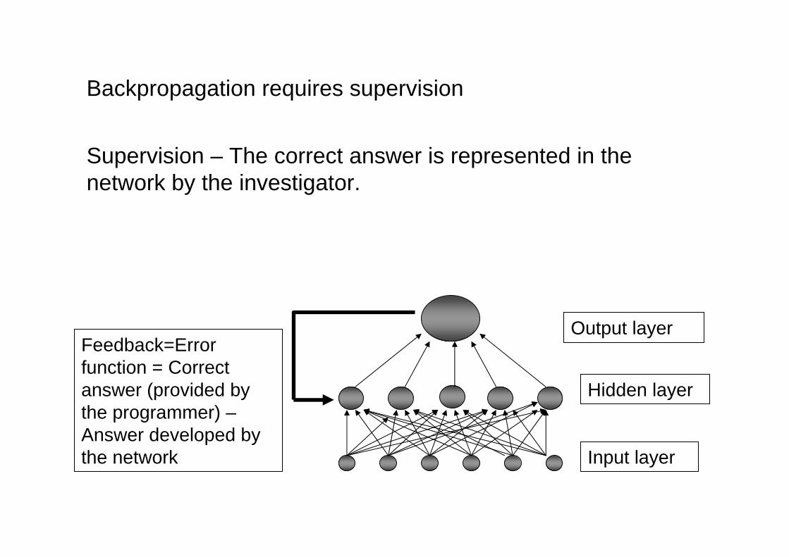
Backpropagation requires supervision

Supervision – The correct answer is represented in the network by the investigator.

Input layer

Hidden layer

Output layerFeedback=Errorfunction = Correct answer (provided by the programmer) –Answer developed by the network

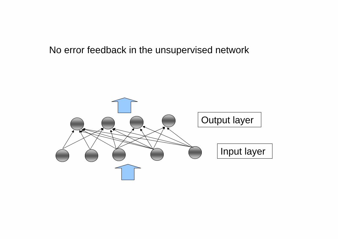
No error feedback in the unsupervised network

Input layer

Output layer

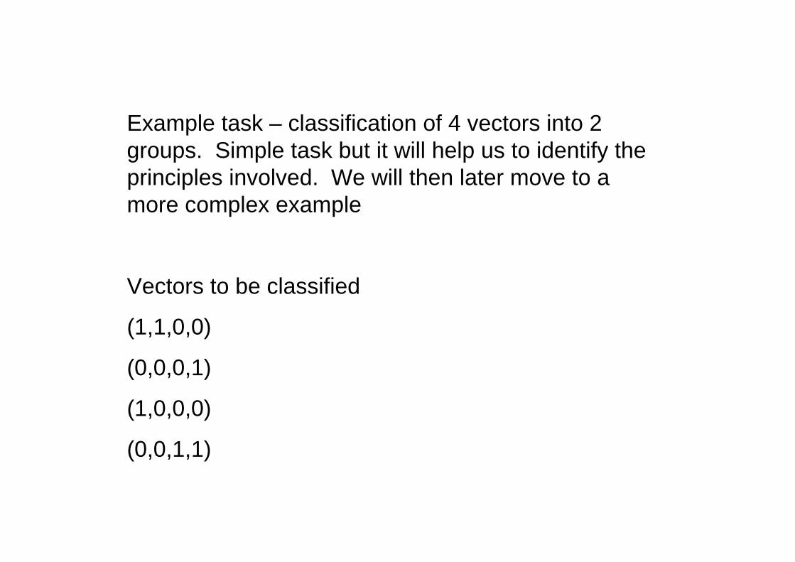
Example task – classification of 4 vectors into 2 groups. Simple task but it will help us to identify the principles involved. We will then later move to a more complex example

Vectors to be classified

(1,1,0,0)

(0,0,0,1)

(1,0,0,0)

(0,0,1,1)

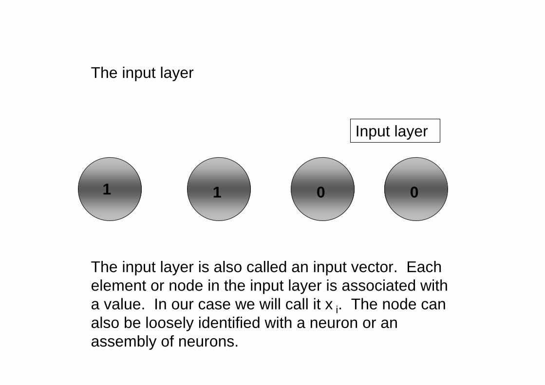
The input layer

The input layer is also called an input vector. Eachelement or node in the input layer is associated witha value. In our case we will call it x i. The node canalso be loosely identified with a neuron or an assembly of neurons.

Input layer

1 1 0 0

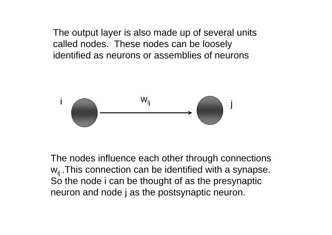
The output layer is also made up of several unitscalled nodes. These nodes can be looselyidentified as neurons or assemblies of neurons

The nodes influence each other through connections wij .This connection can be identified with a synapse. So the node i can be thought of as the presynapticneuron and node j as the postsynaptic neuron.

i jwij

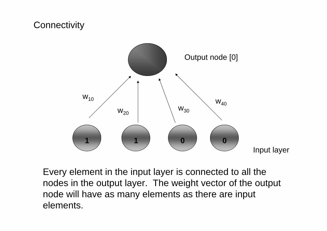
Connectivity

Every element in the input layer is connected to all the nodes in the output layer. The weight vector of the output node will have as many elements as there are input elements.

Input layer

Output node [0]

w10

1 1 0 0

w20w30

w40

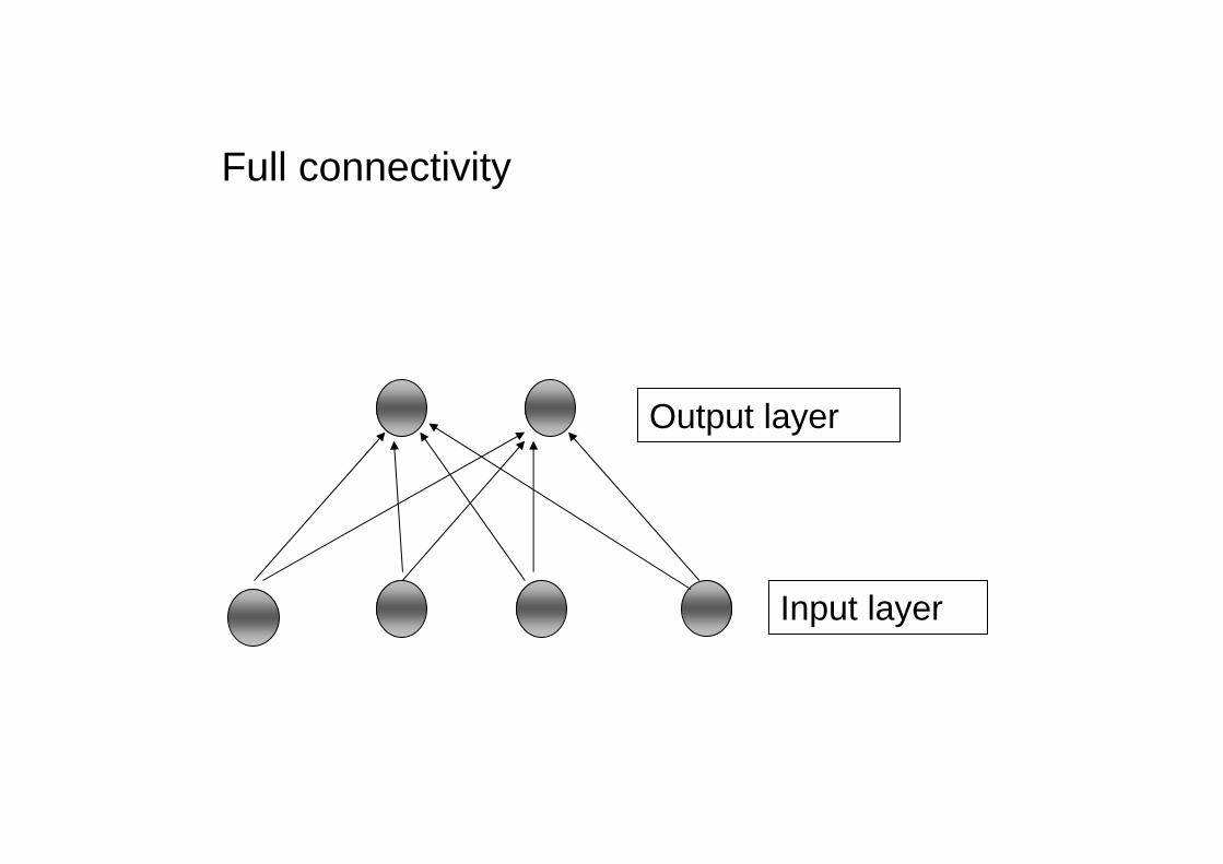
Full connectivity

Input layer

Output layer

When using a Kohonen network (SOM) there are alwaystwo phases

• Training phase – synaptic weights are changed to match input

• Testing phase – synaptic weights stay fixed. We test the performance of the network.

TRAINING PHASE

Each node becomes associated with one input pattern or one category of inputs through a process of weightchange. The weights are gradually changed to more resemble the input vector that it has finally come to represent.

Training phase

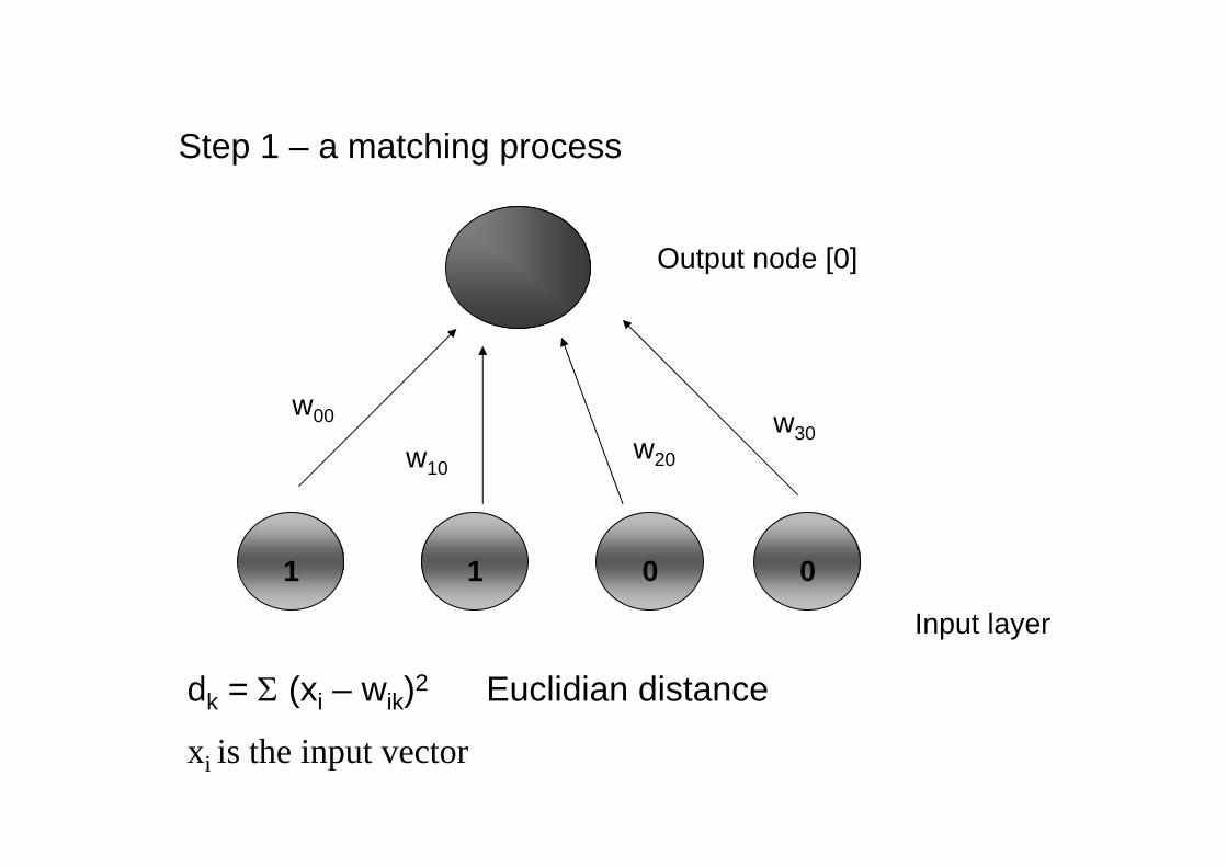
Step 1 – a matching process

dk = (xi – wik)2 Euclidian distance

xi is the input vector

Input layer

Output node [0]

w00

1 1 0 0

w10w20

w30

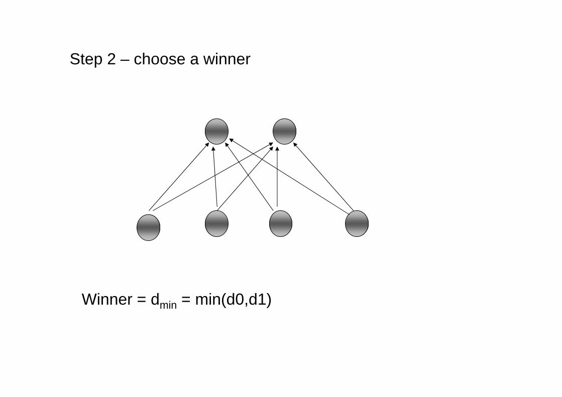
Step 2 – choose a winner

Winner = dmin = min(d0,d1)

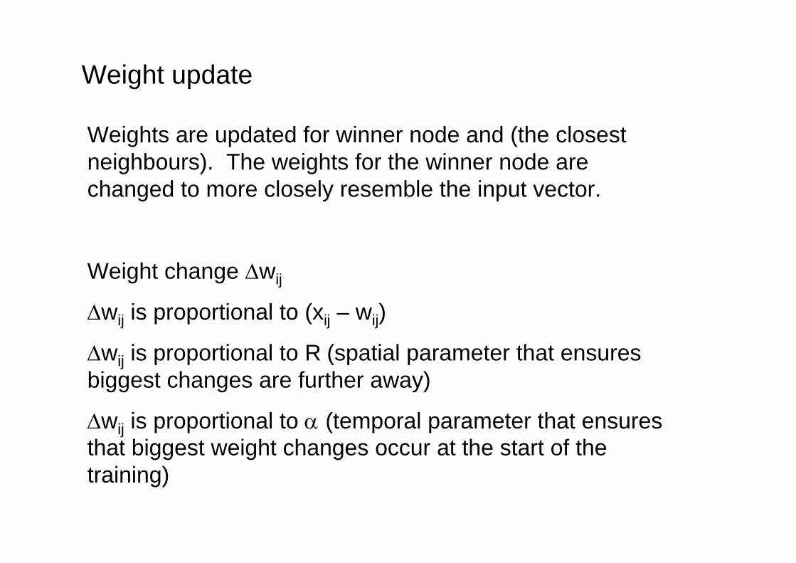
Weight update

Weights are updated for winner node and (the closestneighbours). The weights for the winner node are changed to more closely resemble the input vector.

Weight change wij

wij is proportional to (xij – wij)

wij is proportional to R (spatial parameter that ensuresbiggest changes are further away)

wij is proportional to (temporal parameter that ensuresthat biggest weight changes occur at the start of the training)

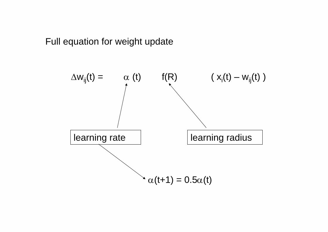
Full equation for weight update

wij(t) = (t) f(R) ( xi(t) – wij(t) )

learning rate learning radius

(t+1) = 0.5(t)

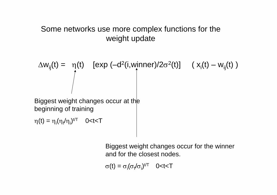
Some networks use more complex functions for the weight update

wij(t) = (t) [exp (–d2(i,winner)/22(t)] ( xi(t) – wij(t) )

Biggest weight changes occur at the beginning of training

(t) = i(f/i)t/T 0<t<T

Biggest weight changes occur for the winner and for the closest nodes.

(t) = i(f/i)t/T 0<t<T

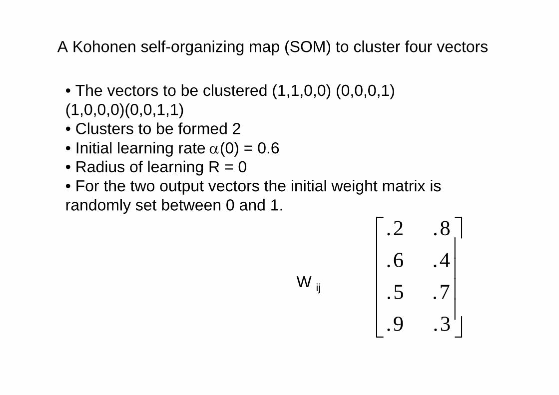
A Kohonen self-organizing map (SOM) to cluster four vectors

• The vectors to be clustered (1,1,0,0) (0,0,0,1) (1,0,0,0)(0,0,1,1)• Clusters to be formed 2• Initial learning rate (0) = 0.6• Radius of learning R = 0• For the two output vectors the initial weight matrix israndomly set between 0 and 1.

3.9.7.5.4.6.8.2.

W ij

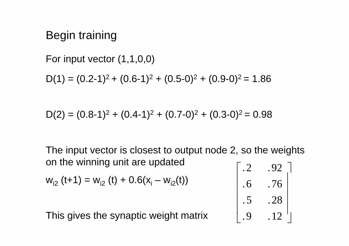
Begin training

For input vector (1,1,0,0)

D(1) = (0.2-1)2 + (0.6-1)2 + (0.5-0)2 + (0.9-0)2 = 1.86

D(2) = (0.8-1)2 + (0.4-1)2 + (0.7-0)2 + (0.3-0)2 = 0.98

The input vector is closest to output node 2, so the weightson the winning unit are updated

wi2 (t+1) = wi2 (t) + 0.6(xi – wi2(t))

This gives the synaptic weight matrix

12.9.28.5.76.6.92.2.

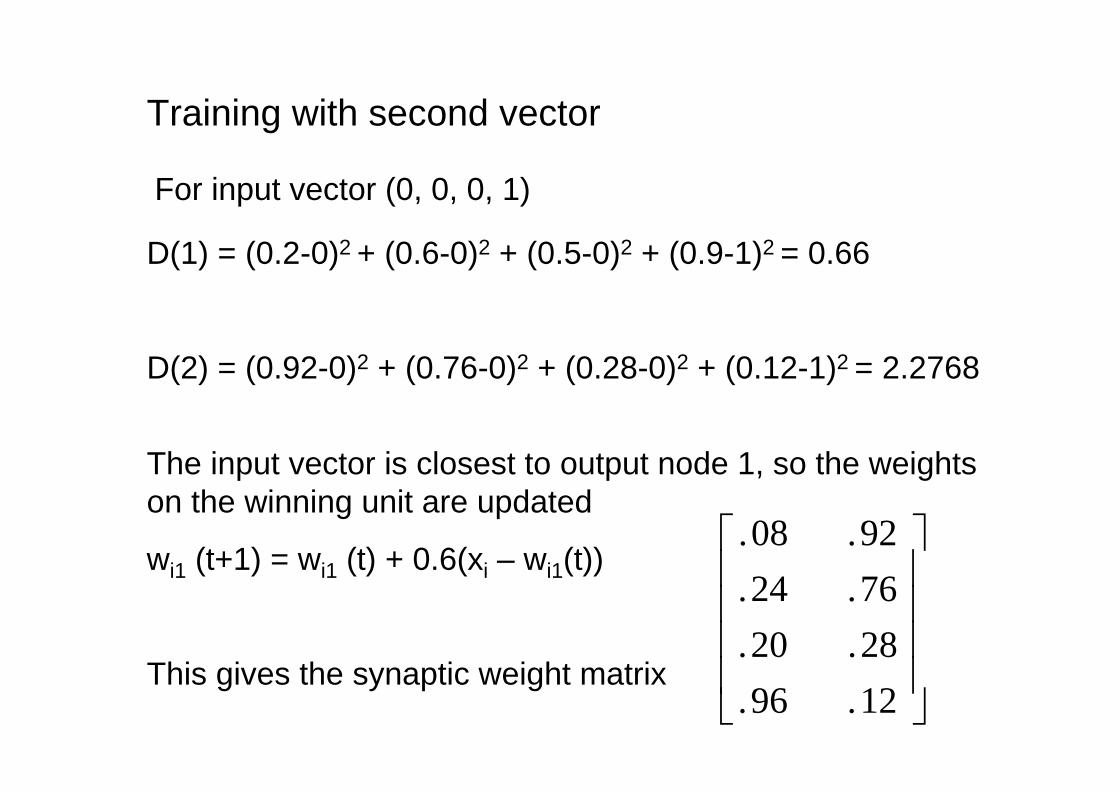
Training with second vector

For input vector (0, 0, 0, 1)

D(1) = (0.2-0)2 + (0.6-0)2 + (0.5-0)2 + (0.9-1)2 = 0.66

D(2) = (0.92-0)2 + (0.76-0)2 + (0.28-0)2 + (0.12-1)2 = 2.2768

The input vector is closest to output node 1, so the weightson the winning unit are updated

wi1 (t+1) = wi1 (t) + 0.6(xi – wi1(t))

This gives the synaptic weight matrix

12.96.28.20.76.24.92.08.

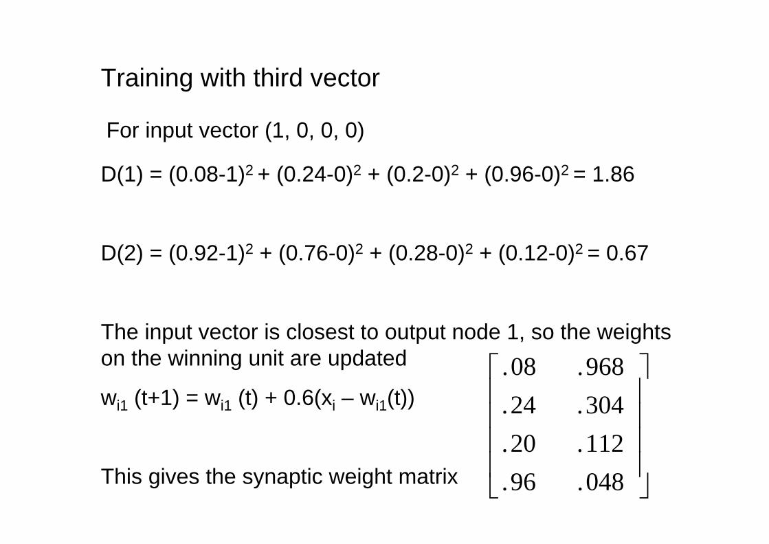
Training with third vector

For input vector (1, 0, 0, 0)

D(1) = (0.08-1)2 + (0.24-0)2 + (0.2-0)2 + (0.96-0)2 = 1.86

D(2) = (0.92-1)2 + (0.76-0)2 + (0.28-0)2 + (0.12-0)2 = 0.67

The input vector is closest to output node 1, so the weightson the winning unit are updated

wi1 (t+1) = wi1 (t) + 0.6(xi – wi1(t))

This gives the synaptic weight matrix

048.96.112.20.304.24.968.08.

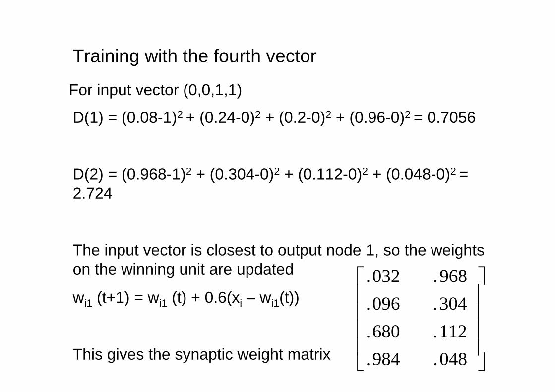
Training with the fourth vector

For input vector (0,0,1,1)

D(1) = (0.08-1)2 + (0.24-0)2 + (0.2-0)2 + (0.96-0)2 = 0.7056

D(2) = (0.968-1)2 + (0.304-0)2 + (0.112-0)2 + (0.048-0)2 = 2.724

The input vector is closest to output node 1, so the weightson the winning unit are updated

wi1 (t+1) = wi1 (t) + 0.6(xi – wi1(t))

This gives the synaptic weight matrix

048.984.112.680.304.096.968.032.

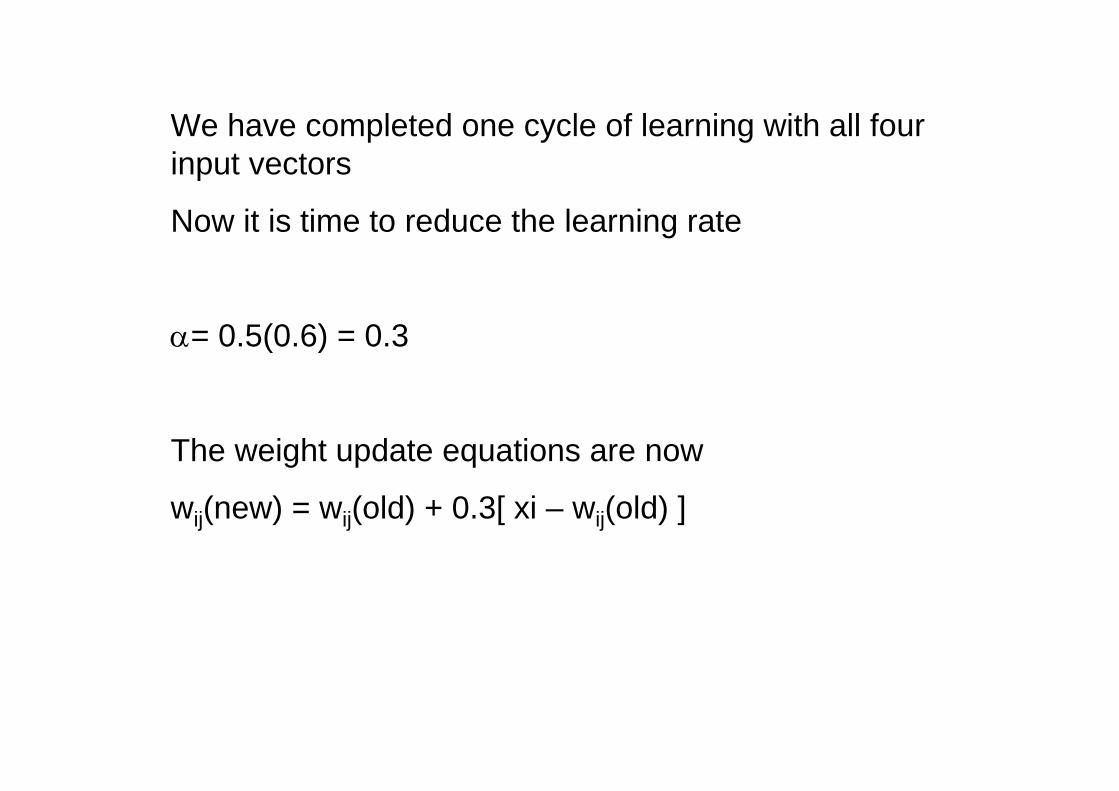
We have completed one cycle of learning with all four input vectors

Now it is time to reduce the learning rate

= 0.5(0.6) = 0.3

The weight update equations are now

wij(new) = wij(old) + 0.3[ xi – wij(old) ]

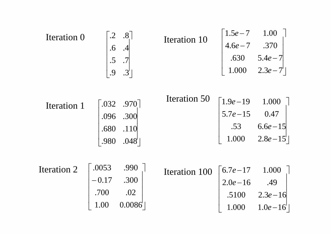
Iteration 0

Iteration 1

Iteration 2

Iteration 10

Iteration 50

Iteration 100

3.9.7.5.4.6.8.2.

048.980.110.680.300.096.970.032.

0086.000.102.700.300.17.0990.0053.

73.2000.174.5630.

370.76.400.175.1

ee

ee

158.2000.1156.653.

47.0157.5000.1199.1

ee

ee

160.1000.1163.25100.

49.160.2000.1177.6

ee

ee

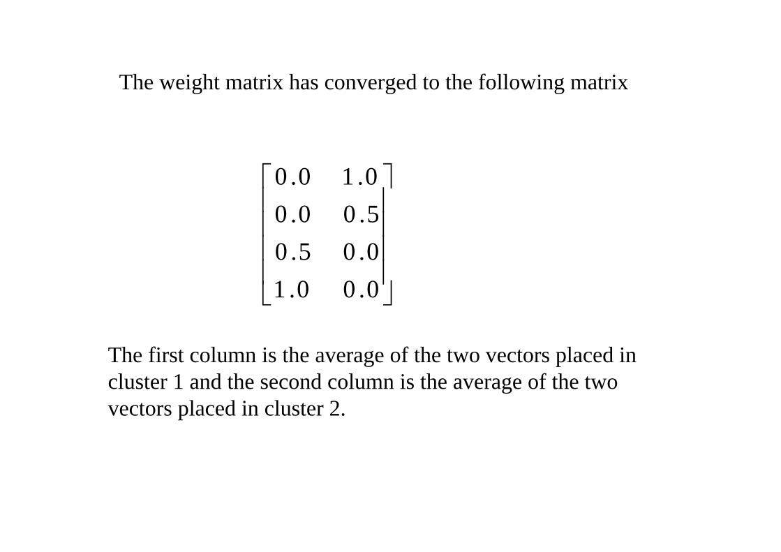
The weight matrix has converged to the following matrix

0.00.10.05.05.00.00.10.0

The first column is the average of the two vectors placed in cluster 1 and the second column is the average of the twovectors placed in cluster 2.

TESTING PHASE

In the testing phase the weights are fixed. With the weights that were obtained in the training phase, youcan now test each vector. If the training wassuccessful, the right node should light up for the right input vector.

In the testing phase, the Euclidian distance iscalculated between input vector and weight vector. The node with the shortest distance is the winner.

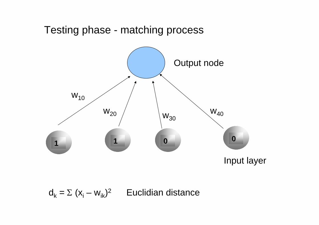
Testing phase - matching process

1 1 0 0

Input layer

Output node

w10

w20 w30w40

dk = (xi – wik)2 Euclidian distance

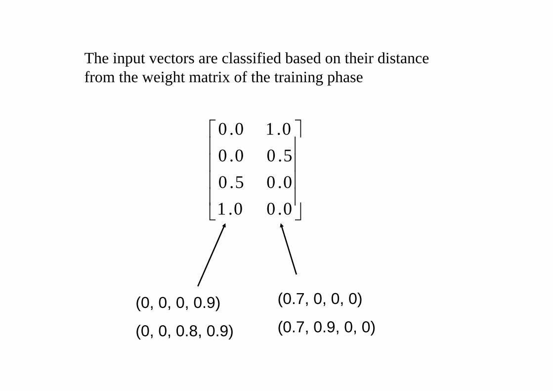
The input vectors are classified based on their distance from the weight matrix of the training phase

0.00.10.05.05.00.00.10.0

(0, 0, 0, 0.9)

(0, 0, 0.8, 0.9)

(0.7, 0, 0, 0)

(0.7, 0.9, 0, 0)

Just a fake example. Things should becomeclearer with a real application

e.g. the classification of characters with differentfonts.

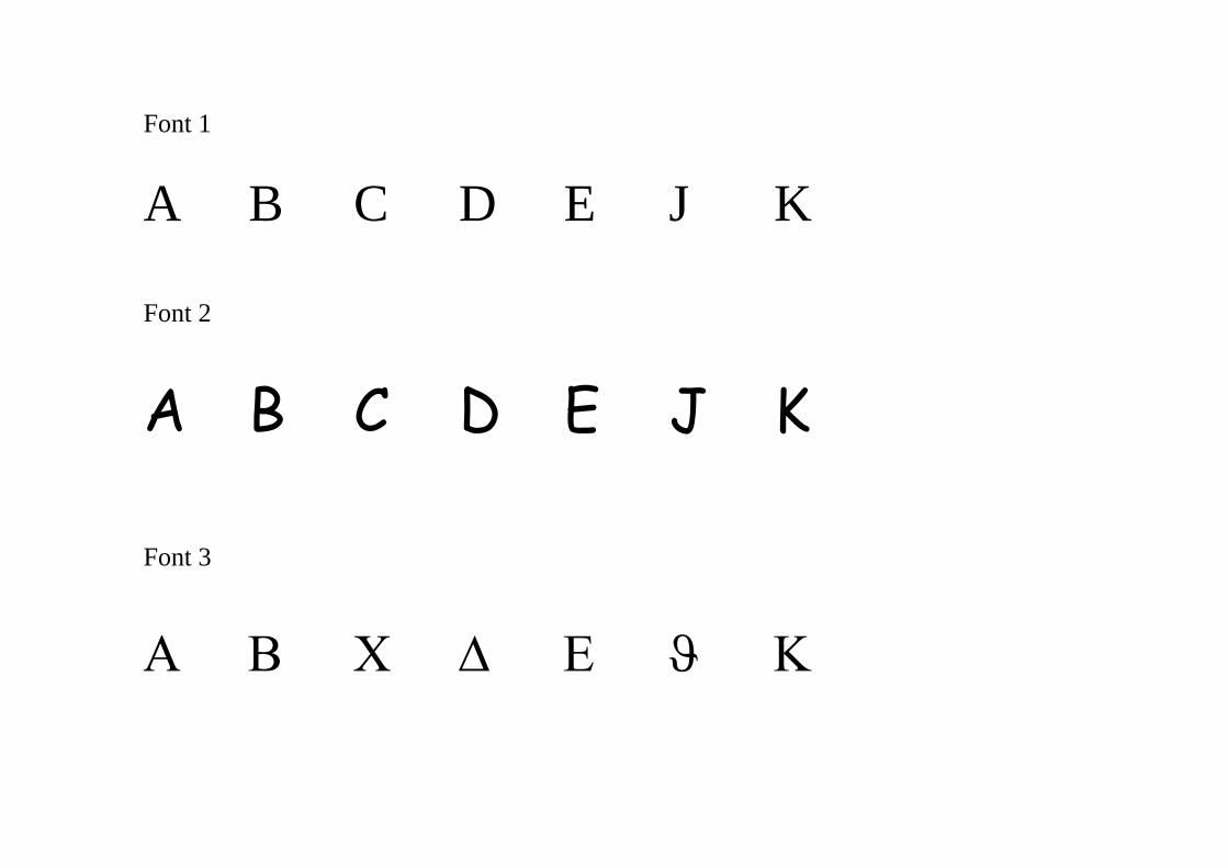
Font 1

A B C D E J K

Font 2

A B C D E J K

Font 3

The role of network geometry

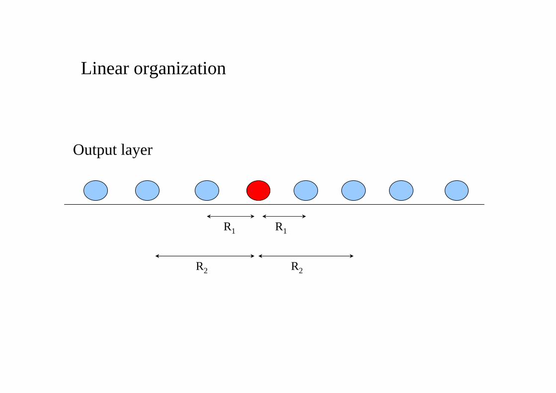
Linear organization

Output layer

R1 R1

R2 R2

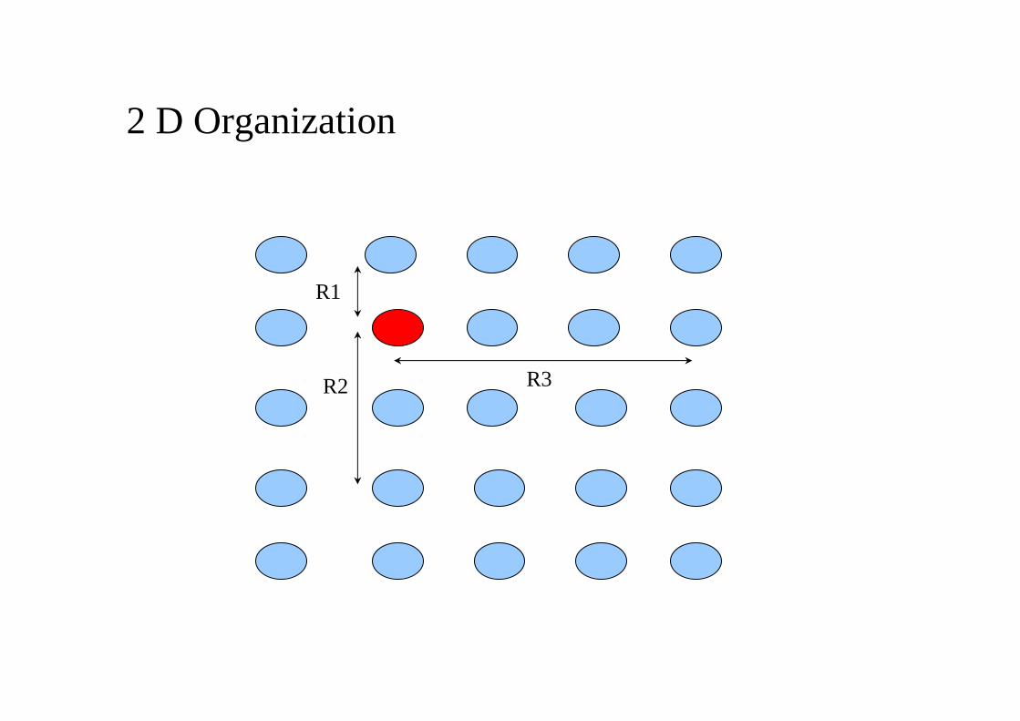
2 D Organization

R1

R2 R3

A Kohonen network with 25 nodes was used to classify the 21 characters with different fonts. In each example the learningrate was reduced linearly from 0.6 to a final value of 0.01. Wewill take a look at the role of network geometry in the classification.

The role of network geometry

A SOM to cluster letters from different fonts: no topological structure

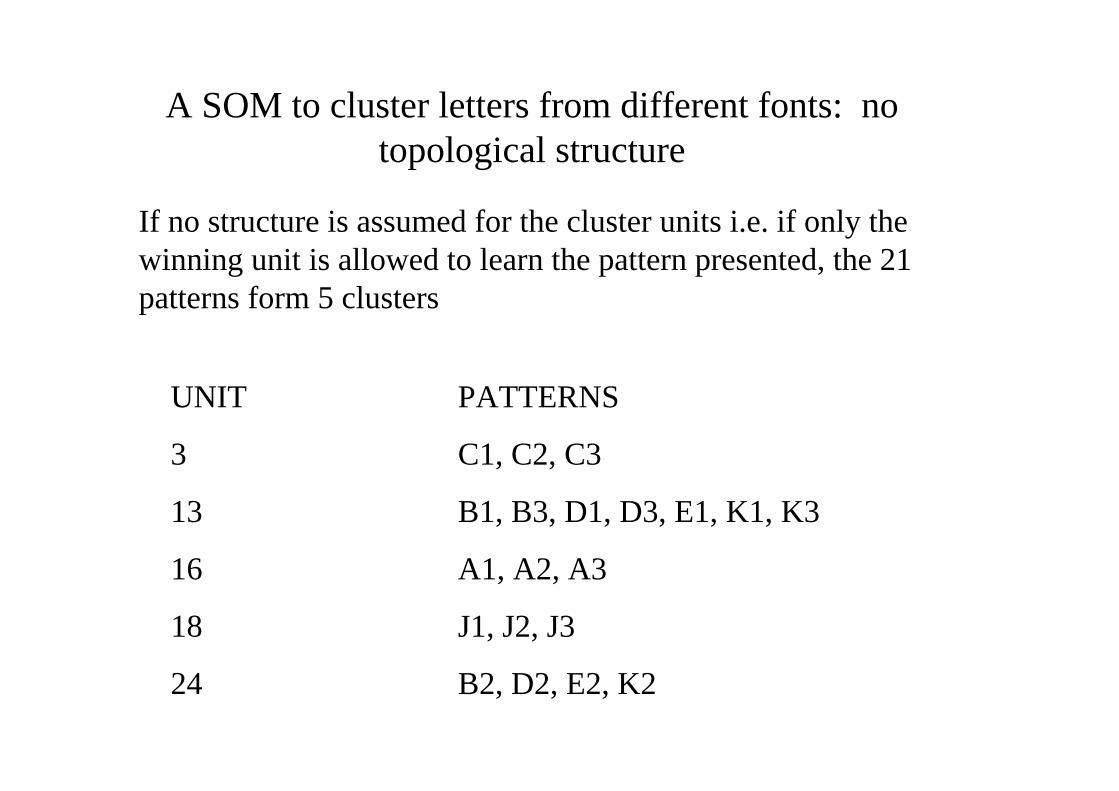
If no structure is assumed for the cluster units i.e. if only the winning unit is allowed to learn the pattern presented, the 21 patterns form 5 clusters

UNIT PATTERNS

3 C1, C2, C3

13 B1, B3, D1, D3, E1, K1, K3

16 A1, A2, A3

18 J1, J2, J3

24 B2, D2, E2, K2

A SOM to cluster letters from different fonts: linearstructure

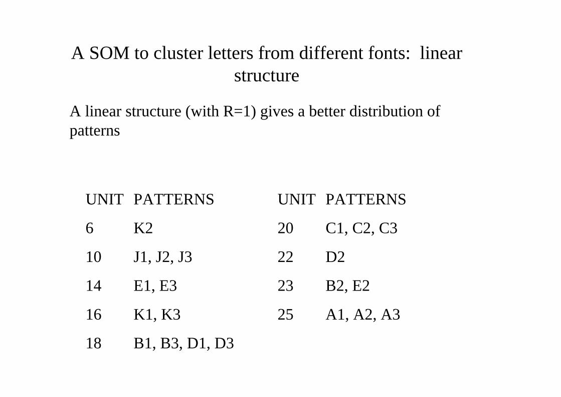
A linear structure (with R=1) gives a better distribution of patterns

UNIT PATTERNS UNIT PATTERNS

6 K2 20 C1, C2, C3

10 J1, J2, J3 22 D2

14 E1, E3 23 B2, E2

16 K1, K3 25 A1, A2, A3

18 B1, B3, D1, D3

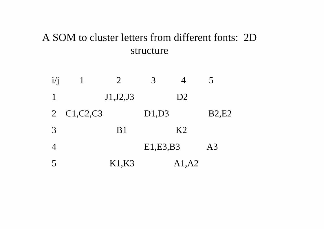
A SOM to cluster letters from different fonts: 2D structure

i/j 1 2 3 4 5

1 J1,J2,J3 D2

2 C1,C2,C3 D1,D3 B2,E2

3 B1 K2

4 E1,E3,B3 A3

5 K1,K3 A1,A2

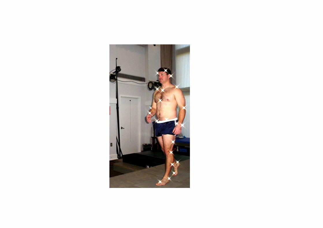
The use of neural networks in orderto analyze kinematic data from 3D

gait analysis

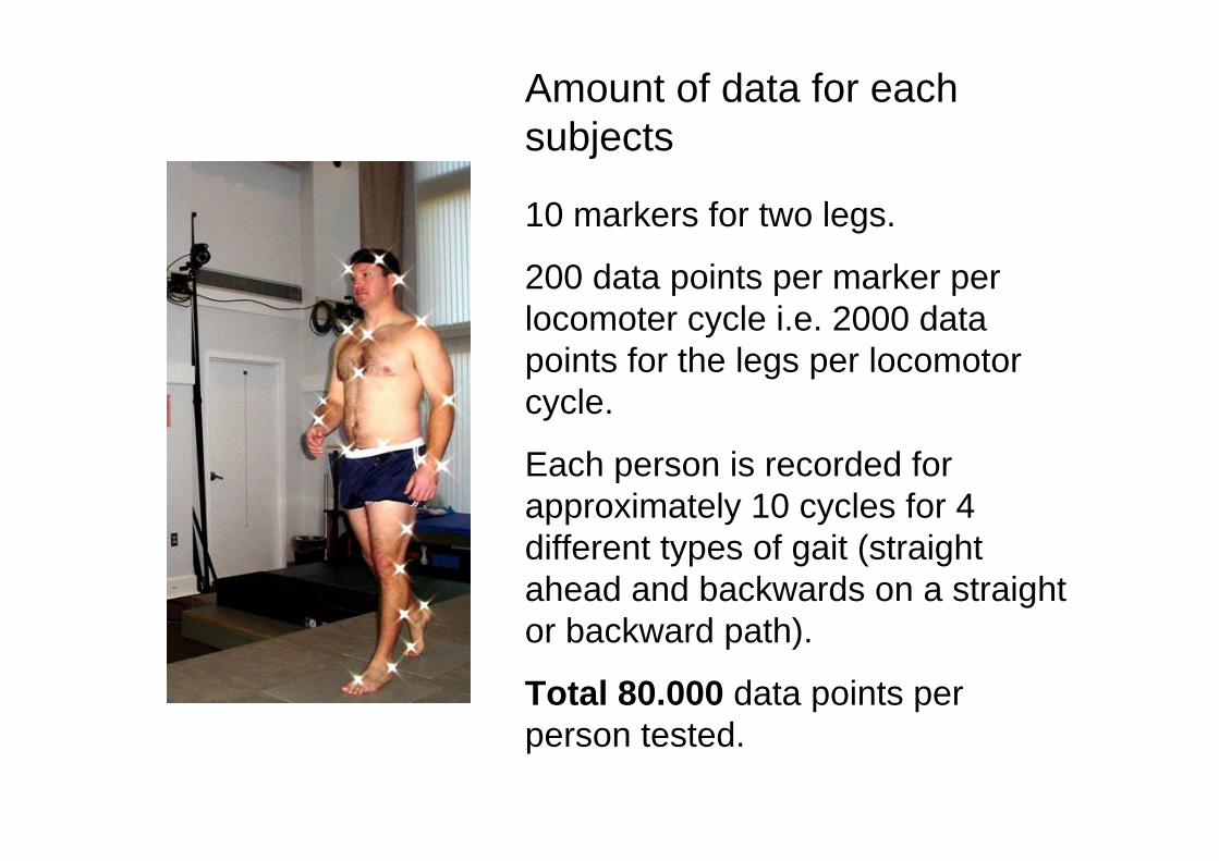
10 markers for two legs.

200 data points per marker per locomoter cycle i.e. 2000 data points for the legs per locomotorcycle.

Each person is recorded for approximately 10 cycles for 4 different types of gait (straight ahead and backwards on a straight or backward path).

Total 80.000 data points per person tested.

Amount of data for eachsubjects

Many neuromuscular disorders createproblems with gait

• Parkinsonism

• Various myopathies

• Peripheral nerve disorders (eg diabetes)

• Problems at the neuromuscular junctione.g. myasthenia gravis

• Cerebellar disorders

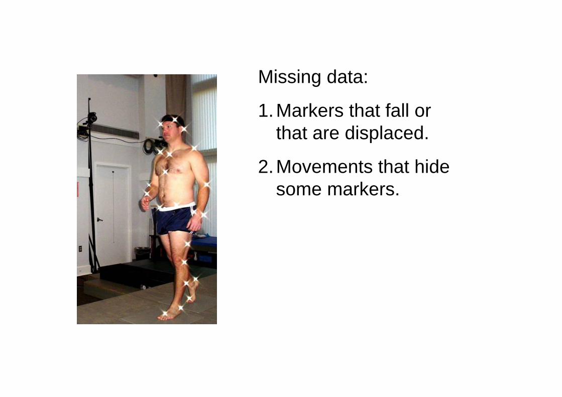
Missing data:

1.Markers that fall or that are displaced.

2.Movements that hidesome markers.

The classification of locomotor disorders

An ongoing project at the laboratoryINSERMU887 is the construction of neural networks in order to classify and to studylocomotive disorders.

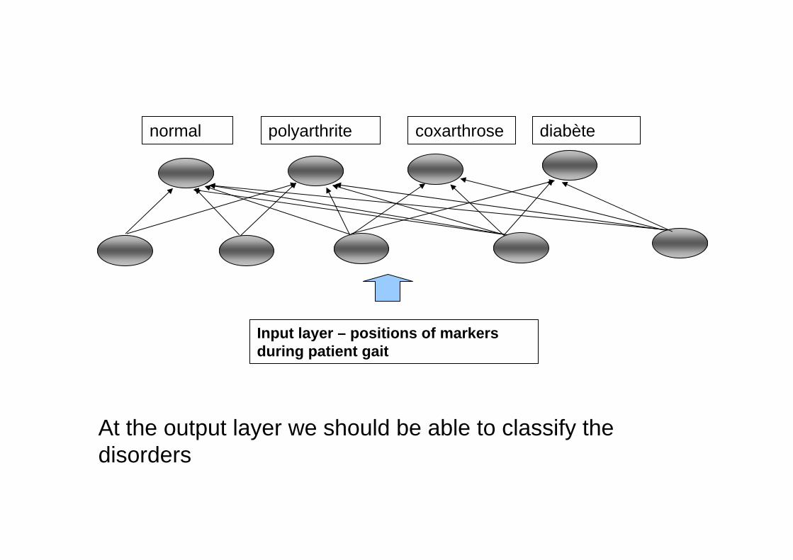
Input layer – positions of markers during patient gait

normal polyarthrite coxarthrose diabète

At the output layer we should be able to classify the disorders