Artificial Neural Networks : An Introduction G.Anuradha.
78
Artificial Neural Networks : An Introduction G.Anuradha
-
Upload
catherine-cooper -
Category
Documents
-
view
234 -
download
3
Transcript of Artificial Neural Networks : An Introduction G.Anuradha.

Artificial Neural Networks : An Introduction
G.Anuradha

Learning Objectives
• Fundamentals of ANN
• Comparison between biological neuron and artificial neuron
• Basic models of ANN
• Different types of connections of NN, Learning and activation function
• Basic fundamental neuron model-McCulloch-Pitts neuron and Hebb network
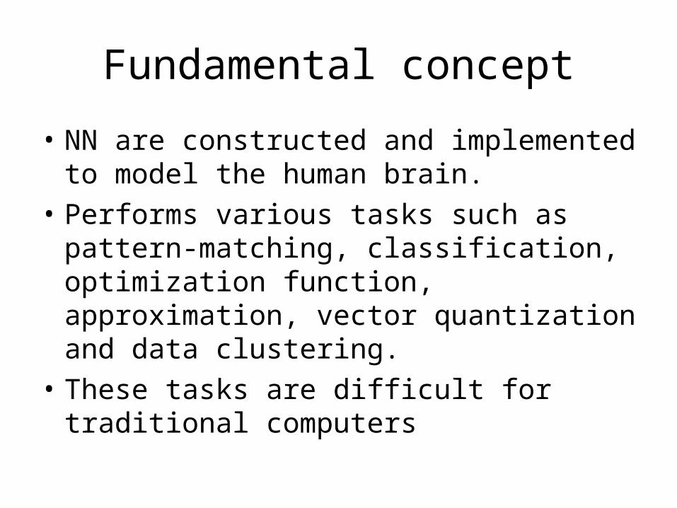
Fundamental concept
• NN are constructed and implemented to model the human brain.
• Performs various tasks such as pattern-matching, classification, optimization function, approximation, vector quantization and data clustering.
• These tasks are difficult for traditional computers

ANN
• ANN posess a large number of processing elements called nodes/neurons which operate in parallel.
• Neurons are connected with others by connection link.
• Each link is associated with weights which contain information about the input signal.
• Each neuron has an internal state of its own which is a function of the inputs that neuron receives- Activation level

Artificial Neural Networks
x1
x2
X1
X2
w1
w2
Y ynX
1 1 2 2iny x w x w
( )iny f y

Information flow in nervous system

Biological Neural Network

Neuron and a sample of pulse train

Biological Neuron• Has 3 parts
– Soma or cell body:- cell nucleus is located– Dendrites:- nerve connected to cell body– Axon: carries impulses of the neuron
• End of axon splits into fine strands• Each strand terminates into a bulb-like organ called synapse• Electric impulses are passed between the synapse and dendrites• Synapses are of two types
– Inhibitory:- impulses hinder the firing of the receiving cell– Excitatory:- impulses cause the firing of the receiving cell
• Neuron fires when the total of the weights to receive impulses exceeds the threshold value during the latent summation period
• After carrying a pulse an axon fiber is in a state of complete nonexcitability for a certain time called the refractory period.

Characteristics of ANN
• Neurally implemented mathematical model• There exist a highly interconnected processing
units called neurons• Interconnections with their weighted linkages
hold information• ANN have the ability to learn, recall, generalize
by adjustment of weights• Computational power is by collective behavior
and no single neuron carries specific information
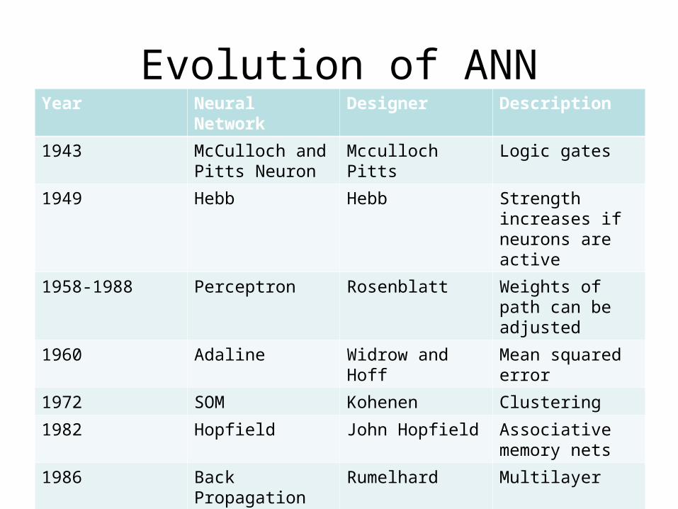
Evolution of ANNYear Neural Network Designer Description
1943 McCulloch and Pitts Neuron
Mcculloch Pitts Logic gates
1949 Hebb Hebb Strength increases if neurons are active
1958-1988 Perceptron Rosenblatt Weights of path can be adjusted
1960 Adaline Widrow and Hoff Mean squared error
1972 SOM Kohenen Clustering
1982 Hopfield John Hopfield Associative memory nets
1986 Back Propagation Rumelhard Multilayer
1987-90 ART Carpenter Used for both binary and analog

McCulloch-Pitts Neuron Model

Features of McCulloch-Pitts model
• Allows binary 0,1 states only
• Operates under a discrete-time assumption
• Weights and the neurons’ thresholds are fixed in the model and no interaction among network neurons
• Just a primitive model

General symbol of neuron consisting of processing node and
synaptic connections

Neuron Modeling for ANN
Is referred to activation function. Domain is set of activation values net.
Scalar product of weight and input vector
Neuron as a processing node performs the operation of summation of its weighted input.

Activation function
• Bipolar binary and unipolar binary are called as hard limiting activation functions used in discrete neuron model
• Unipolar continuous and bipolar continuous are called soft limiting activation functions are called sigmoidal characteristics.

Activation functionsBipolar continuous
Bipolar binary functions

Activation functionsUnipolar continuous
Unipolar Binary

Common models of neurons
Binary perceptrons
Continuous perceptrons

Comparison between brain verses computer Brain ANN
Speed Few ms. Few nano sec. massive ||el processing
Size and complexity 1011 neurons & 1015
interconnectionsDepends on designer
Storage capacity Stores information in its interconnection or in synapse.
No Loss of memory
Contiguous memory locations
loss of memory may happen sometimes.
Tolerance Has fault tolerance No fault tolerance Inf gets disrupted when interconnections are disconnected
Control mechanism Complicated involves chemicals in biological neuron
Simpler in ANN

Basic models of ANN
Basic Models of ANN
Interconnections Learning rules Activation function

Classification based on interconnections
Network architecture is the arrangement of neurons to form layers and connection patterns formed within and between layers

Single layer Feedforward Network

Feedforward Network
• Its output and input vectors are respectively
• Weight wij connects the i’th neuron with j’th input. Activation rule of ith neuron is
where
EXAMPLE

Multilayer feed forward network
Can be used to solve complicated problems

Example of feedforward network

Feedback networkWhen outputs are directed back as inputs to same or preceding layer nodes it results in the formation of feedback networks. The input is given only once and then removed

Categories of feedback
• Discrete feedback
• Continuous feedback

Discrete feedback network
• The mapping of o(t) with o(t+∆) is given by
• The time step is unity and time instances are indexed as positive integers.
• For discrete feedback network
• A system with discrete time inputs and discrete data representation is called an automaton. (Recurrent Neural networks)

Recurrent n/ws
• Single node with own feedback
• Competitive nets
• Single-layer recurrent nts
• Multilayer recurrent networks
Feedback networks with closed loop are called Recurrent Networks. The response at the k+1’th instant depends on the entire history of the network starting at k=0. Automaton: A system with discrete time inputs and a discrete data representation is called an automaton
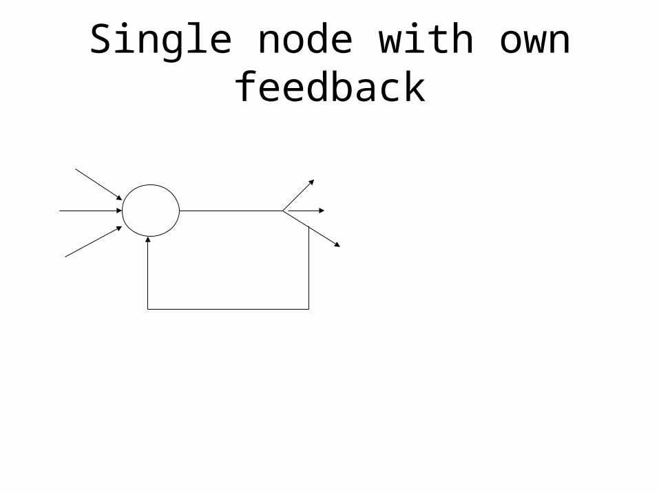
Single node with own feedback

Single layer Recurrent Networks

Competitive networks

Lateral feedbackIf the feedback of the output of the processing elements is directed back as input to the processing elements in the same layer then it is called lateral feedback

Continuous feedback networks
• Continuous time networks employ neurons with continuous activation function.
• Used in electrical circuits. Relation between resistance, inductance and capacitance

Basic models of ANN
Basic Models of ANN
Interconnections Learning rules Activation function

Learning
• It’s a process by which a NN adapts itself to a stimulus by making proper parameter adjustments, resulting in the production of desired response
• Two kinds of learning– Parameter learning:- connection weights are
updated– Structure Learning:- change in network
structure

Training
• The process of modifying the weights in the connections between network layers with the objective of achieving the expected output is called training a network.
• This is achieved through– Supervised learning– Unsupervised learning– Reinforcement learning

Classification of learning
• Supervised learning
• Unsupervised learning
• Reinforcement learning

Supervised Learning
• Child learns from a teacher
• Each input vector requires a corresponding target vector.
• Training pair=[input vector, target vector]
NeuralNetwork
W
ErrorSignal
Generator
X
(Input)
Y
(Actual output)
(Desired Output)
Error
(D-Y) signals

Supervised learning contd.
Supervised learning does minimization of error

Unsupervised Learning
• How a fish or tadpole learns• All similar input patterns are grouped together as
clusters.• If a matching input pattern is not found a new
cluster is formed

Unsupervised learning
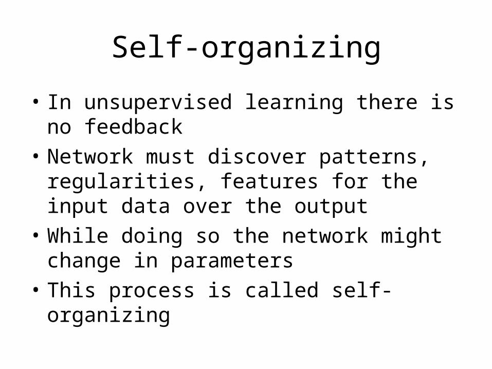
Self-organizing
• In unsupervised learning there is no feedback
• Network must discover patterns, regularities, features for the input data over the output
• While doing so the network might change in parameters
• This process is called self-organizing

Reinforcement Learning
NNW
ErrorSignal
Generator
X
(Input)
Y
(Actual output)
Error
signals R
Reinforcement signal

When Reinforcement learning is used?
• If less information is available about the target output values (critic information)
• Learning based on this critic information is called reinforcement learning and the feedback sent is called reinforcement signal
• Feedback in this case is only evaluative and not instructive
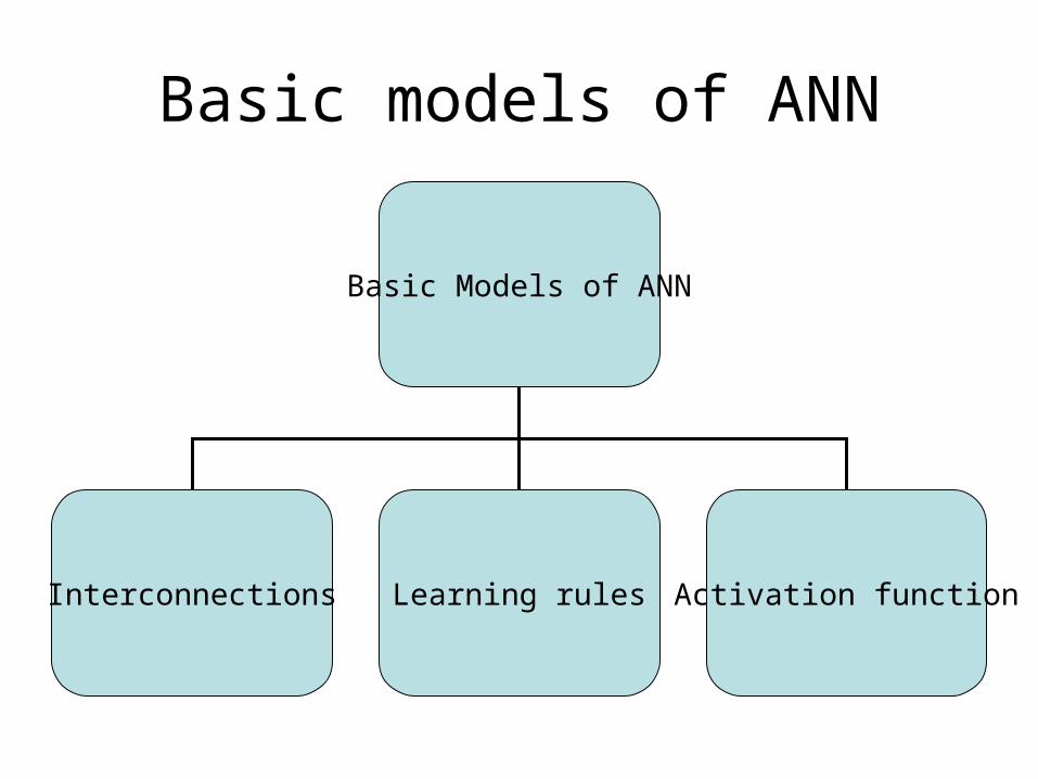
Basic models of ANN
Basic Models of ANN
Interconnections Learning rules Activation function
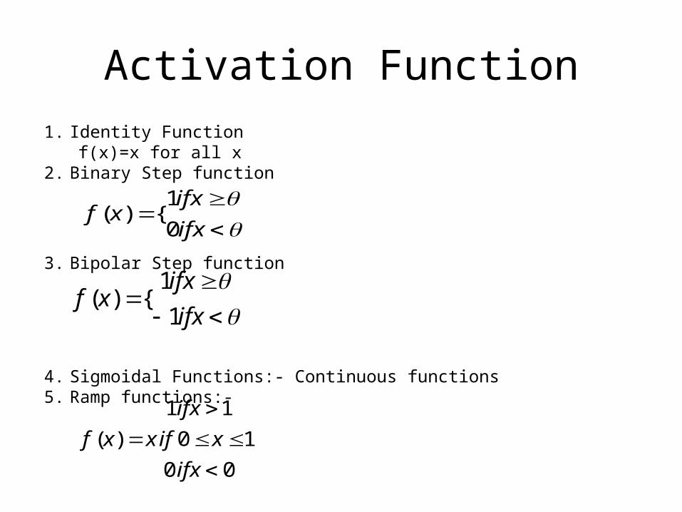
1. Identity Functionf(x)=x for all x
2. Binary Step function
3. Bipolar Step function
4. Sigmoidal Functions:- Continuous functions 5. Ramp functions:-
Activation Function
ifx
ifxxf
0
1{)(
ifx
ifxxf
1
1{)(
00
10
11
)(
ifx
xifx
ifx
xf
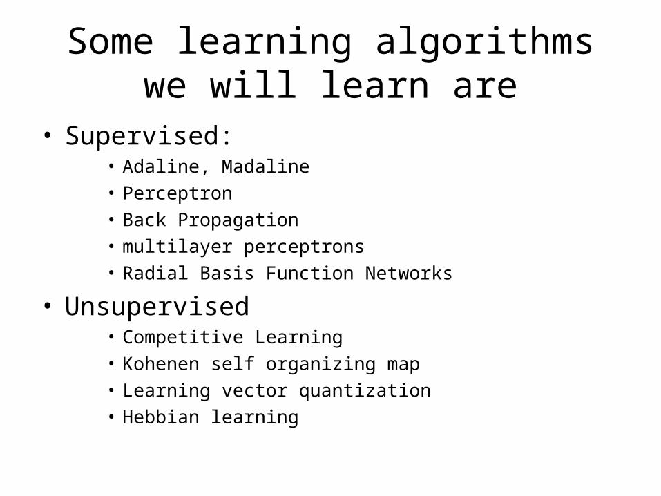
Some learning algorithms we will learn are
• Supervised:• Adaline, Madaline• Perceptron• Back Propagation• multilayer perceptrons• Radial Basis Function Networks
• Unsupervised• Competitive Learning• Kohenen self organizing map• Learning vector quantization• Hebbian learning

Neural processing
• Recall:- processing phase for a NN and its objective is to retrieve the information. The process of computing o for a given x
• Basic forms of neural information processing– Auto association– Hetero association– Classification

Neural processing-Autoassociation
• Set of patterns can be stored in the network
• If a pattern similar to a member of the stored set is presented, an association with the input of closest stored pattern is made
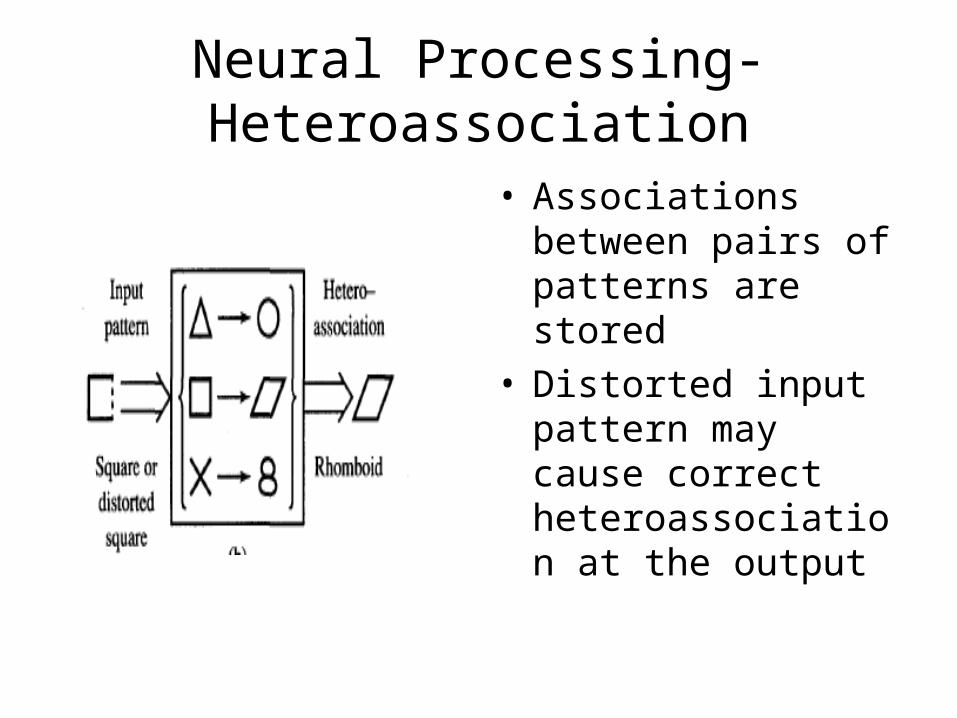
Neural Processing- Heteroassociation
• Associations between pairs of patterns are stored
• Distorted input pattern may cause correct heteroassociation at the output

Neural processing-Classification
• Set of input patterns is divided into a number of classes or categories
• In response to an input pattern from the set, the classifier is supposed to recall the information regarding class membership of the input pattern.

Important terminologies of ANNs
• Weights
• Bias
• Threshold
• Learning rate
• Momentum factor
• Vigilance parameter
• Notations used in ANN

Weights
• Each neuron is connected to every other neuron by means of directed links
• Links are associated with weights
• Weights contain information about the input signal and is represented as a matrix
• Weight matrix also called connection matrix

Weight matrix
W=1
2
3
.
.
.
.
.
T
T
T
T
n
www
w
=
11 12 13 1
21 22 23 2
1 2 3
...
...
..................
...................
...
m
m
n n n nm
w w w ww w w w
w w w w

Weights contd…• wij –is the weight from processing element ”i” (source node)
to processing element “j” (destination node)
X1
1
XiYj
Xn
w1j
wij
wnj
bj
0
0 0 1 1 2 2
01
1
....
n
i ijinji
j j j n nj
n
j i iji
n
j i ijinji
y x w
x w x w x w x w
w x w
y b x w

Activation Functions
• Used to calculate the output response of a neuron.
• Sum of the weighted input signal is applied with an activation to obtain the response.
• Activation functions can be linear or non linear• Already dealt
– Identity function– Single/binary step function– Discrete/continuous sigmoidal function.

Bias
• Bias is like another weight. Its included by adding a component x0=1 to the input vector X.
• X=(1,X1,X2…Xi,…Xn)
• Bias is of two types– Positive bias: increase the net input– Negative bias: decrease the net input

Why Bias is required?
• The relationship between input and output given by the equation of straight line y=mx+c
X YInput
C(bias)
y=mx+C

Threshold
• Set value based upon which the final output of the network may be calculated
• Used in activation function• The activation function using threshold can be
defined as
ifnet
ifnetnetf
1
1)(
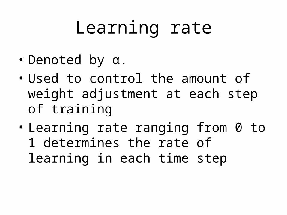
Learning rate
• Denoted by α.
• Used to control the amount of weight adjustment at each step of training
• Learning rate ranging from 0 to 1 determines the rate of learning in each time step
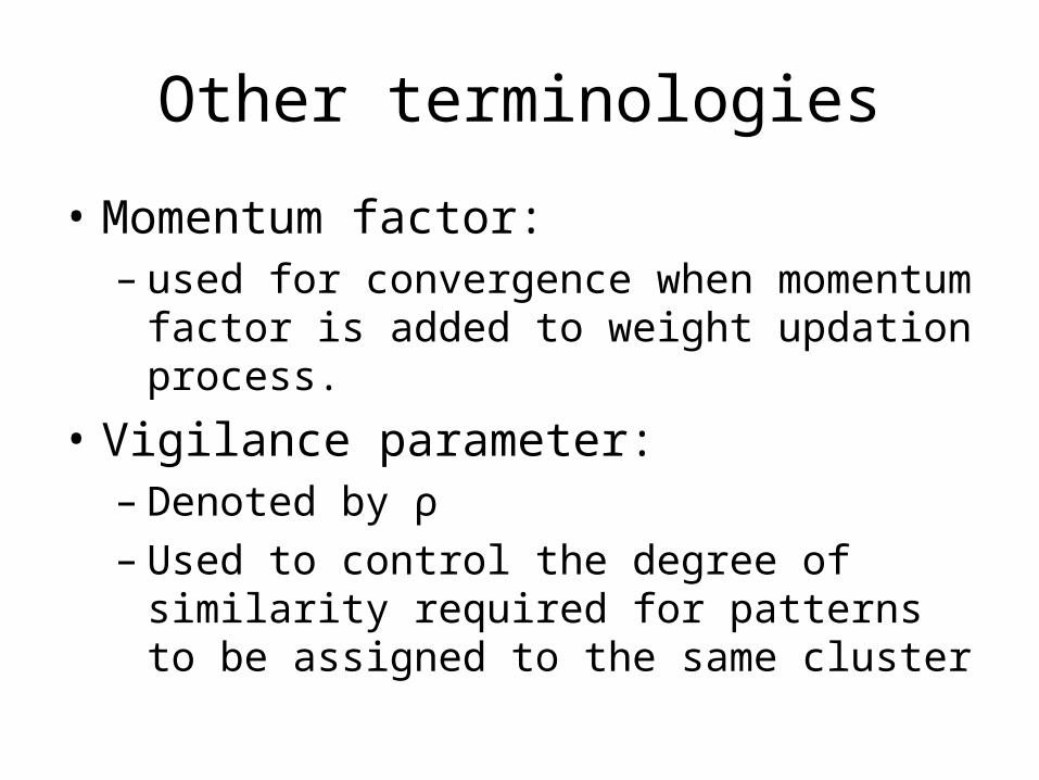
Other terminologies
• Momentum factor: – used for convergence when momentum factor
is added to weight updation process.
• Vigilance parameter:– Denoted by ρ– Used to control the degree of similarity
required for patterns to be assigned to the same cluster

Neural Network Learning rules
c – learning constant

Hebbian Learning Rule
• The learning signal is equal to the neuron’s output
FEED FORWARD UNSUPERVISED LEARNING

Features of Hebbian Learning
• Feedforward unsupervised learning
• “When an axon of a cell A is near enough to exicite a cell B and repeatedly and persistently takes place in firing it, some growth process or change takes place in one or both cells increasing the efficiency”
• If oixj is positive the results is increase in weight else vice versa


Perceptron Learning rule• Learning signal is the difference between the
desired and actual neuron’s response• Learning is supervised

Delta Learning Rule
• Only valid for continuous activation function• Used in supervised training mode• Learning signal for this rule is called delta• The aim of the delta rule is to minimize the error over all training
patterns

Delta Learning Rule Contd.
Learning rule is derived from the condition of least squared error.
Calculating the gradient vector with respect to wi
Minimization of error requires the weight changes to be in the negative gradient direction
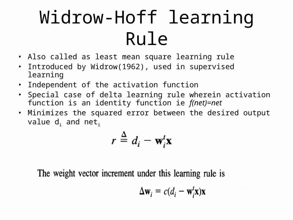
Widrow-Hoff learning Rule
• Also called as least mean square learning rule• Introduced by Widrow(1962), used in supervised learning• Independent of the activation function• Special case of delta learning rule wherein activation function is an
identity function ie f(net)=net• Minimizes the squared error between the desired output value di
and neti

Winner-Take-All learning rules

Winner-Take-All Learning rule Contd…
• Can be explained for a layer of neurons• Example of competitive learning and used for
unsupervised network training• Learning is based on the premise that one of the
neurons in the layer has a maximum response due to the input x
• This neuron is declared the winner with a weight


Summary of learning rules
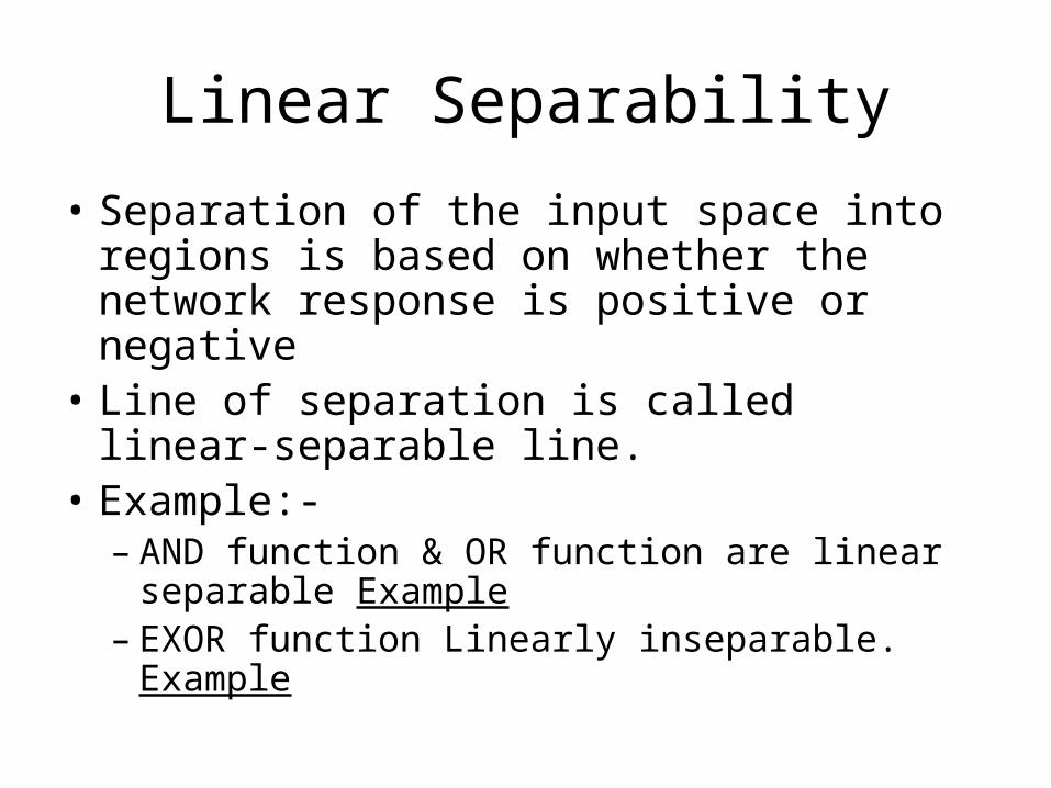
Linear Separability
• Separation of the input space into regions is based on whether the network response is positive or negative
• Line of separation is called linear-separable line.
• Example:-– AND function & OR function are linear
separable Example– EXOR function Linearly inseparable. Example

Hebb Network
• Hebb learning rule is the simpliest one• The learning in the brain is performed by the
change in the synaptic gap• When an axon of cell A is near enough to excite
cell B and repeatedly keep firing it, some growth process takes place in one or both cells
• According to Hebb rule, weight vector is found to increase proportionately to the product of the input and learning signal.
yxoldwneww iii )()(

Flow chart of Hebb training algorithm
Start
Initialize Weights
For Each
s:t
Activate inputxi=si
1
1
Activate outputy=t
Weight updateyxoldwneww iii )()(
Bias updateb(new)=b(old) + y
Stop
y
n