Artificial Neural Networks 1

Tim de Bruin Robert Babuska

t.d.debruin@tudelft.nl

Knowledge-Based Control Systems (SC42050)Cognitive Robotics

3mE, Delft University of Technology, The Netherlands

05-03-2018

Outline

This lecture:

1 Introduction to artificial neural networks

2 Simple networks & approximation properties

3 Deep Learning

4 Optimization

Next lecture:

1 Regularization & Validation

2 Specialized network architectures

3 Beyond supervised learning

4 Examples

2 / 49

Outline

1 Introduction to artificial neural networks

2 Simple networks & approximation properties

3 Deep Learning

4 Training

3 / 49

Motivation: biological neural networks

� Humans are able to process complex tasks efficiently (perception,pattern recognition, reasoning, etc.).

� Learning from examples.

� Adaptivity and fault tolerance.

In engineering applications:

� Nonlinear approximation and classification.

� Learning and adaptation from data (black-box models).

� High dimensional inputs / outputs

4 / 49

Biological neuron

dendrites

soma

axon

synapse

5 / 49

Artificial neuron

...

x1

xp

x2

w1

wp

w2z

v

xi : ith input of the neuronwi : adaptive weight (synaptic strength) for xiz : weighted sum of inputs: z = ∑p

i=1wixi = wTxσ(z) : activation functionv : output of the neuron

6 / 49

Activation functions

Purpose: transformation of the input space (squeezing).Two main types:

� Projection functions: threshold function, piece-wise linearfunction, tangent hyperbolic, sigmoidal, rectified linear, ...function:

σ(z) = 1/(1 + exp(−2z))

� Kernel functions (radial basis functions):

σ(x) = exp (−(x − c)2/s2)

7 / 49

Activation functions: some common choices

1

z

σ( )z

0

-1

z

σ( )z

0

1

z

σ( )z

0

1

z

σ( )z

0

-1

1

Sigmoid: σ(z) = 11+e−z

Tangent hyperbolic: σ(z) = 21+e−2z − 1

Rectified Linear Unit (ReLU): σ(z) =⎧⎪⎪⎨⎪⎪⎩

0 if z < 0z if z ≥ 0

Exponential Linear Unit (ELU): σ(z) =⎧⎪⎪⎨⎪⎪⎩

z if z > 0α(ez − 1) if z ≤ 0

8 / 49

Outline

1 Introduction to artificial neural networks

2 Simple networks & approximation properties

3 Deep Learning

4 Training

9 / 49

Neural Network: Interconnected Neurons

Multi-layer ANN

Single-layer recurrent ANN

10 / 49

Feedforward neural network example

x1

.

.

.

y1

xp

vm

yn

hidden layer output layerinput layer

wp

x2

v1

.

.

.

wh

w11wh

w11wo

wmnwo

m

11 / 49

Feedforward neural network example (cont’d)

1 Activation of hidden-layer neuron j :

zj =p

∑i=1

whij xi + bhj

2 Output of hidden-layer neuron j :

vj = σ (zj)

3 Output of output-layer neuron l :

yl =h

∑j=1

wojl vj + b

ol

12 / 49

Function approximation with neural nets: examples

y = wo1 tanh (wh

1 x + bh1) +wo2 tanh (wh

2 x + bh2)

Transformationthrough tanh

x

v

0

v2v1

tanh(z1)tanh(z )2

Summation of

neuron outputs

Activation (weightedsummation)

z

x0

w1hx b1

h+w2hx b2

h+

z1 z2

y

x0

w1ov1 w2

ov2

w1ov1 w2

ov2+

Warping space

Need for nonlinearities

13 / 49

Input–Output Mapping

Matrix notation:

Z = XbWh

V = σ(Z)Y = VbW

o

with Xb = [X 1] and Vb = [V 1].

Compact formula (1-layer feedforward net):

Y = [σ([X 1]Wh) 1]Wo

14 / 49

Approximation properties of neural nets

[Cybenko, 1989]: A feedforward neural net with at least one hiddenlayer can approximate any continuous nonlinear function Rp → Rn

arbitrarily well, provided that sufficient number of hidden neurons areavailable (not constructive).

15 / 49

Approximation properties of neural nets

[Barron, 1993]: A feedforward neural net with one hidden layer withsigmoidal activation functions can achieve an integrated squared errorof the order

J = O (1h)

independently of the dimension of the input space p, where h denotesthe number of hidden neurons.

For a basis function expansion (polynomial, trigonometric expansion,singleton fuzzy model, etc.) with h terms, in which only the parametersof the linear combination are adjusted

J = O ( 1

h2/p)

16 / 49

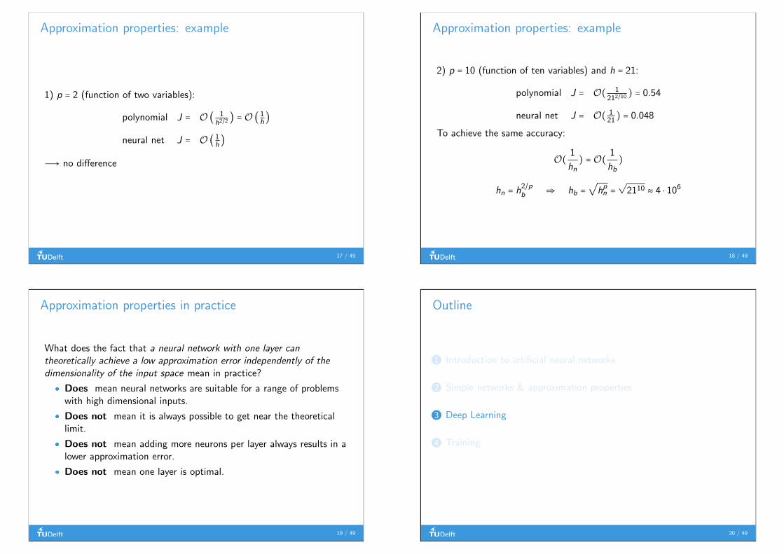
Approximation properties: example

1) p = 2 (function of two variables):

polynomial J = O ( 1h2/2) = O ( 1h)

neural net J = O ( 1h)

Ð→ no difference

17 / 49

Approximation properties: example

2) p = 10 (function of ten variables) and h = 21:

polynomial J = O( 1212/10

) = 0.54

neural net J = O( 121) = 0.048

To achieve the same accuracy:

O( 1hn) = O( 1

hb)

hn = h2/pb ⇒ hb =√hpn =

√2110 ≈ 4 ⋅ 106

18 / 49

Approximation properties in practice

What does the fact that a neural network with one layer cantheoretically achieve a low approximation error independently of thedimensionality of the input space mean in practice?

� Does mean neural networks are suitable for a range of problemswith high dimensional inputs.

� Does not mean it is always possible to get near the theoreticallimit.

� Does not mean adding more neurons per layer always results in alower approximation error.

� Does not mean one layer is optimal.

19 / 49

Outline

1 Introduction to artificial neural networks

2 Simple networks & approximation properties

3 Deep Learning

4 Training

20 / 49

Manifold hypothesis

For many problems defined in very high dimensional spaces, the data ofinterest lie on low dimensional manifolds embedded in the highdimensional space. Demo: moving over a faces manifold

21 / 49

More examples of lower dimensional representations

512 dimensions

"A train traveling down tracks next to a forest."

640 x 360 x 3 = 691.200 dimensions

1000

dimensions

German

Image

English

English

1

1D. P. Kingma and M. Welling (2013). “Auto-encoding variational bayes”. In: arXiv preprint arXiv:1312.6114;O. Vinyals, A. Toshev, S. Bengio, and D. Erhan (2015). “Show and tell: A neural image caption generator”. In:Proceedings of the IEEE Conference on Computer Vision and Pattern Recognition, pp. 3156–3164; A. Radford, L. Metz,and S. Chintala (2015). “Unsupervised representation learning with deep convolutional generative adversarial networks”.In: arXiv preprint arXiv:1511.06434; M.-T. Luong, Q. V. Le, I. Sutskever, O. Vinyals, and L. Kaiser (2015). “Multi-tasksequence to sequence learning”. In: arXiv preprint arXiv:1511.06114

22 / 49

Deep Learning

Output

Input

Hand designed

mapping

Classic

Control

Hand designed

features

learned

mapping

Output

Input

Classic

machine learning

learned

mapping

Output

Input

learned

features

learned

features

...

Deep

learning

23 / 49

Deep Learning - feature hierarchy

unicycle dog

Input

Output

object parts

corners,

contours

edges

2

Year layers

2012 82013 82014 222015 1522016 269

Table: Number of layers in the winningneural network in the imagenetcompetition

2M. D. Zeiler and R. Fergus (2014). “Visualizing and understanding convolutional networks”. In: European conferenceon computer vision. Springer, pp. 818–833

24 / 49

Outline

1 Introduction to artificial neural networks

2 Simple networks & approximation properties

3 Deep Learning

4 TrainingOverviewBack-propagationCost functionsStochastic Gradient Descent

25 / 49

Neural network training

Goal: find the weight vector W that minimizes some cost functionJ(f (x ;W )) for all (especially unseen) inputs x .

Supervised learning example: Make a neural network approximate aknown function x → t by minimizing: J(W ) = 1

2(f (x ;W ) − t)2

26 / 49

Neural network training - general algorithm

1 Initialize W to small random values

2 Repeat until the performance (on a separate test-set) stopsimproving:

1 Forward pass: Given an input x , calculate the neural networkoutput y = f (x ;W ). Then calculate the cost J(y , t) of predicting yinstead of the target output t.

2 Backward pass: Calculate the gradient of the cost with respect to

the weights: ∇J(y(x ;W ), t) = [ ∂J∂w1

, . . . , ∂J∂wn]T

3 Optimization step: Change the weights based on the gradient toreduce the cost.

27 / 49

Supervised learning

Input Output

error

System

-

28 / 49

Learning in feedforward nets

1 Feedforward computation. From the inputs proceed through thehidden layers to the output.

Z = XbWh, Xb = [X 1]

V = σ(Z)

Y = VbWo , Vb = [V 1]

29 / 49

Learning in feedforward nets

2 Weight adaptation. Compare the net output with the desiredoutput:

E = T −Y

Adjust the weights such that the following cost function isminimized:

J(w) = 1

2

N

∑k=1

l

∑j=1

e2kj

w = [Wh Wo]

(This is the empirical loss: the loss over the examples in the dataset. We actually want to minimize the loss over the trueunderlying distribution of examples. We come back to this difference in the next lecture.)

30 / 49

Output-layer weights example

Neuron

ev2

y-

d

J1/2 e2

vn

v1

wnwo

w2wo

w1wo tCost function

J = 1

2e2, e = t − y , y =∑

j

woj vj

∂J

∂woj

= ∂J

∂e⋅ ∂e∂y⋅ ∂y

∂woj

= −vje

31 / 49

Hidden-layer weights example

hidden layer

output layer

x2

e2vz

xp

el

x1

e1

wpwh

w2wh

w1wh

wl

wo

w2wo

w1wo

∂J

∂whij

= ∂J

∂vj⋅∂vj

∂zj⋅∂zj

∂whij

= −xi ⋅ σ′j(zj) ⋅∑l

elwojl

∂J

∂vj= ∑

l

−elwojl ,

∂vj

∂zj= σ′j(zj),

∂zj

∂whij

= xi

32 / 49

Back-propagating further

x1

x3w32

x2

v1

wh1

w11wh1

ww11

o

w21wo

h2

v2h2

v1h1

v2h1

J(t,y)

tww11

o

w21wo

∂J∂wh1

11

= ( ∂J∂vh2

1

∂vh21

∂vh11

+ ∂J∂vh2

2

∂vh22

∂vh11

) ∂vh11

∂wh11 1

33 / 49

Cost functions

Cost function term types:

� Classification

� Regression

� Regularization (next lecture)

Two main criteria:

1 The minimum of the cost function w∗ = argminw J(f (w)) shouldcorrespond to desirable behavior.examples:

� J(y , t) = ∣∣y − t ∣∣2 : y = f (x ;w∗)→ mean t for each x� J(y , t) = ∣∣y − t ∣∣1 : y = f (x ;w∗)→ median of t for each x

2 The error gradient should be informative.

34 / 49

Informative gradients

x2

yz

xp

x1

wpw

w2w

w1w

J(y,t)

tOutput neuron

�J/�y�J/�z

�J/�Xp

�J/�X2

�J/�X1

�J/�Wp

�J/�W1

The cost function J and nonlinearity σ of the output neurons should becompatible.

35 / 49

Informative gradients

x2

yz

xp

x1

wpw

w2w

w1w

J(y,t)

tOutput neuron

�J/�y�J/�z

�J/�Xp

�J/�X2

�J/�X1

�J/�Wp

�J/�W1

� linear output, MSE:

y = z , J = 1

2(y − t)2 → ∂J

∂z= ∂J

∂y

∂y

∂z= (y − t) ⋅ 1

� sigmoidal output, MSE:

y = 1

1 + e−z, J = 1

2(y − t)2 → ∂J

∂z= ∂J

∂y

∂y

∂z=

(y − t) ⋅ y(1 − y) = (y2 − ty)(1 − y)

36 / 49

Informative gradients

x2

yz

xp

x1

wpw

w2w

w1w

J(y,t)

tOutput neuron

�J/�y�J/�z

�J/�Xp

�J/�X2

�J/�X1

�J/�Wp

�J/�W1

� linear output, MSE: ∂J∂z = y − t

� sigmoidal output, MSE: ∂J∂z = (y

2 − ty)(1 − y)� sigmoidal output, negative log likelihood:

y = 1

1 + e−z, J = −t ln(y) − (1 − t) ln(1 − y) → ∂J

∂z= ∂J

∂y=

−ty+ 1 − t1 − y

⋅ y(1 − y) = y − t

37 / 49

Informative gradients

x2

yz

xp

x1

wpw

w2w

w1w

J(y,t)

tOutput neuron

�J/�y�J/�z

�J/�Xp

�J/�X2

�J/�X1

�J/�Wp

�J/�W1

38 / 49

(Stochastic) Gradient Descent

Update rule for the weights:

wn+1 = wn − αn∇J(wn)

with the gradient ∇J(wn)

∇J(w) = ( ∂J

∂w1,∂J

∂w2, . . . ,

∂J

∂wM)T

� Gradient Descent: use ∇J(w) = 1K ∑

Ki=1(

∂J(ti ,f (xi ;W ))∂W )

with K = the size of the database

� Stochastic Gradient Descent: use∇J(w) = 1

k ∑ki=1(

∂J(ti ,f (xi ;W ))∂W ) with k << K the batch size

39 / 49

Stochastic Gradient Descent

∇J(w) = 1k ∑

ki=1(

∂J(ti ,f (xi ;W ))∂W ) with k << K

In practice: k ≈ 100 − 102, K ≈ 104 − 109.

The xi , ti data points in the batches should be independent andidentically distributed (i.i.d.).

What might go wrong when learning online?

40 / 49

What step size?

w( 1)n+ w

J(w)

w( )n

41 / 49

Second-order gradient methods

J(w) ≈ J(w0) +∇J(w0)T (w −w0) +1

2(w −w0)TH(w0)(w −w0)

where H(w0) is the Hessian in w0.

Update rule for the weights:

wn+1 = wn −H−1(wn)∇J(wn)

42 / 49

Second-order gradient methods

w( 1)n+ w

J(w)

w( )n

43 / 49

Step size per weight

H−1∇J computes a goodstep for each weight, onlyfeasible for (very) smallnetworks.

Can we do better thanGradient Descent withoutusing second orderderivatives?

low learning rate

high learning rate

Gradient Descent

44 / 49

Improvements to SGD

� Momentum: increase step-size if we keep going in the samedirection

v ← βv − α∇Jw ← w + v

� RMSProp: decrease step-size over time, especially if gradients arelarge

r ← γr + (1 − γ)∇J ⊙∇J

w ← w − α√10−6 +

√r⊙∇J

Initialize v, r to 0. Choose β, γ ∈ [0,1)

45 / 49

Improvements to SGD

� ADAM: combine both previous ideas and correct for their initialbias

s← βs + (1 − β)∇Jr ← γr + (1 − γ)∇J ⊙∇J

s← s

1 − βt

r ← r

1 − γt

w ← w − α s√10−6 + r

Initialize s, r to 0. Choose β, γ ∈ [0,1). Common values: β = 0.9, γ = 0.999.

46 / 49

Optimization strategies using only first order gradients

Gradient Descent

Momentum

RMSProp

Adam

47 / 49

Summary artificial neural networks part 1

...

x1

xp

x2

w1

wp

w2

zv

y1

y2

1

z

σ( )z

0

-1

z

σ( )z

0

1

z

σ( )z

0

1

Foward pass:

y = f(x; w)output

network structure

input

input

weights

weights

nonlinearity

48 / 49

Summary artificial neural networks part 1

Backward pass: calculate ∇J and use it in an optimization algorithmto iteratively update the weights of the network to minimize the loss J.

...

x1

xp

x2

w1

wp

w2

zv

J(y,t)

target output

network output

Loss function�J/�y1

�J/�y2

�J/�v�J/�z

�J/�w

�J/�v1

49 / 49